Dynamic Demand-Aware Link Scheduling
for Reconfigurable Datacenters

Abstract

Emerging reconfigurable datacenters allow to dynamically adjust the network topology in a demand-aware manner. These datacenters rely on optical switches which can be reconfigured to provide direct connectivity between racks, in the form of edge-disjoint matchings. While state-of-the-art optical switches in principle support microsecond reconfigurations, the demand-aware topology optimization constitutes a bottleneck.

This paper proposes a dynamic algorithms approach to improve the performance of reconfigurable datacenter networks, by supporting faster reactions to changes in the traffic demand. This approach leverages the temporal locality of traffic patterns in order to update the interconnecting matchings incrementally, rather than recomputing them from scratch. In particular, we present six (batch-)dynamic algorithms and compare them to static ones. We conduct an extensive empirical evaluation on 176 synthetic and 39 real-world traces, and find that dynamic algorithms can both significantly improve the running time and reduce the number of changes to the configuration, especially in networks with high temporal locality, while retaining matching weight.

I Introduction

The performance of many cloud-based applications critically depends on the underlying network, requiring high-throughput datacenter networks which provide extremely large bandwidth [1, 2, 3]. For example, in distributed machine learning and data mining applications that periodically require large data transfers, the network is increasingly becoming a bottleneck. High network throughput requirements are also introduced by today’s trend of resource disaggregation in datacenters, where fast access to remote resources (e.g., GPUs or memory) is critical, and the trend to hardware-driven workloads such as distributed training [1].

The stringent throughput requirements of modern datacenter applications have led researchers to propose innovative datacenter network designs which rely on reconfigurable topologies [4, 5, 6, 7, 8, 9, 10, 11, 12, 13]: emerging optical technologies allow to enhance existing datacenter networks with reconfigurable optical matchings. In particular, optical circuit switches can provide direct connectivity between datacenter racks, in the form of one matching per optical circuit switch. This technology enables demand-aware networks [14]: the optical matchings, and hence the datacenter topology interconnecting the racks, are adjusted depending on the current communication traffic.

Such demand-aware topology optimizations are attractive as datacenter traffic typically features much spatial and temporal structure, and most transmitted bytes belong to a small number of so-called elephant flows [15, 16, 17]. Thus, throughput may be significantly increased by optimizing the topology towards the current traffic matrix and elephant flows. This can be achieved, for example, by providing direct connectivity between frequently communicating racks rather than serving traffic along multiple hops, which introduces a “bandwidth tax” [18, 13].

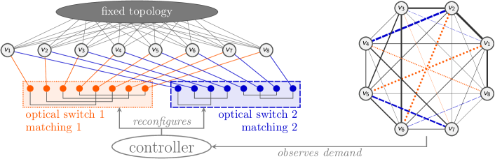
Figure 1: Two optical switches establishing direct connections between nodes $v_{1},\dots,v_{8}$, as instructed by the network controller, and the demand graph with the corresponding two matchings.

However, demand-aware topology optimizations are computationally expensive. In fact, state-of-the-art algorithms [8, 19, 20, 21, 22, 23, 24] to compute optimized demand-aware switch matchings for a given demand matrix can have a running time that is significantly higher than the actual reconfiguration time provided by the state-of-the-art optical technologies (which is in the order of microseconds or even less [25, 26]). Thus, the computation of the demand-aware topology can be the bottleneck for demand-aware datacenter networks.

Formally, the problem of optimizing the topology of a demand-aware network is a novel variant of a matching problem consisting of “heavy” disjoint matchings [25] (see Fig. 1): given $k$ optical switches and a traffic demand (a.k.a. demand matrix) represented as a weighted graph where each node corresponds to a datacenter rack and weighted edges represent demands, compute $k$ (edge-)disjoint matchings of high weight. The weight of these matchings hence corresponds to the amount of traffic which can be offloaded to the reconfigurable network, and hence to the throughput achieved by the datacenter network. In most existing reconfigurable datacenter architectures, including Helios [20], c-Through [22], or recently Google’s Gemini [27], among many others [19, 21, 23, 24], this topology optimization is performed by a centralized software controller. Computing such a set of matchings of maximum weight is NP-hard and cannot be approximated with arbitrary precision for all $k\geq 2$ [28, 25].

The goal of this work is to improve the running time for computing $k$ disjoint matchings to allow datacenter networks to react to changes in the demand more quickly and improve throughput further. Our main idea is as follows: Since traffic exhibits much temporal locality, it can be inefficient to recompute the datacenter topology from scratch for each traffic matrix. Rather, we study dynamic algorithms, i.e., algorithms which update the topology incrementally, as a reaction to shifts in the demand matrix. Besides speeding up the computation, such dynamic algorithms may also require fewer changes in configurations to achieve a given throughput. The latter benefits ongoing flows as fewer of them will be interrupted.

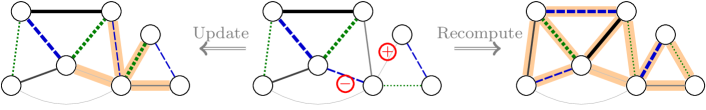
Figure 2: Updating vs. recomputing a solution from scratch for $k=2$: The two matchings are visualized in dotted green and dashed blue, the line width of an edge corresponds to its weight. Shaded edges have been changed.
Center: Initial situation. Two updates arrive, one increases an edge weight , another decreases an edge weight . Left: The result after processing the updates. Only four edges are affected. Right: The potential result after a full recomputation from scratch. The whole network is reconsidered and also unaffected edges may have change, which can be inefficient.

We illustrate our motivation with a simple example network, see also Fig. 2: Assume the communication demand, i.e. edge weight, of a node to two of its neighbors changes. A dynamic algorithm, which processes the updates itself, has the possibility to adjust the configuration locally and to leave most of the old solution untouched. By contrast, a static one, which does a full recomputation from scratch, needs to process the entire network and, as it is unaware of the old configuration, may additionally introduce unnecessary changes. This can negatively affect both the running time of the algorithm and the number of changes to implement on the optical switches.

Thus, we study the following dynamic weighted $k$-disjoint matching problem: Given an undirected graph $G$ with edge weights representing the current communication demands, process a sequence of batch updates, each consisting of a set of (edge) updates, where each (edge) update either inserts or deletes an edge or changes the weight of one edge. The main goal is to process each batch as quickly as possible and deliver an up-to-date configuration, i.e., $k$ edge-disjoint matchings, after each batch such that the total weight is maximized. A secondary goal is to keep the recourse small, i.e., to minimize the number of changes to the matchings.

Contributions

We develop and evaluate a diverse set of algorithmic techniques for the weighted k-disjoint matching problem arising in the context of reconfigurable datacenter networks. Based on the best static algorithms in [25], we design two dynamic algorithms, which process each update individually, three batch-dynamic algorithms, which process a batch of updates collectively, and two hybrid algorithms, which combine subroutines of static and dynamic approaches. Furthermore, we introduce a universal speedup technique that filters out insignificant updates, as well as a universal post-processing routine that ensures an at least $\frac{1}{2}$-approximation of the maximum weight and can also be run standalone. We compare these algorithms and their speedup and postprocessing versions in detail with respect to solution weight, running time, and recourse in theory and practice to the best static algorithms from [25].

Main Experimental Results

Our extensive study on $39$ real-world and $176$ synthetic instances shows that our batch-dynamic and dynamic algorithms can beat the best static algorithm w.r.t. running time and recourse, while essentially retaining the solution weight. The combination of the post-processing and speedup technique proved to be particularly important for the solution weight of the dynamic algorithms. On instances where batches are small, their advantage over static algorithms is even more pronounced. Our two hybrid algorithms successfully combine the advantages of static and dynamic algorithms and are a good general-purpose choice.

We note that our approach is compatible with most existing reconfigurable datacenter architectures, including [20, 22, 19, 21, 23, 24, 29, 30], which can hence directly benefit from these performance improvements. Due to space restrictions, all proofs are omitted.

II Preliminaries

Basics

We model the communication demand between peers as an undirected, weighted graph $G=(V,E,w)$ with node set $V$, edge set $E$, and use $n:=|V|$, $m:=|E|$. The function $w:E\to\mathbb{N}_{0}$ maps each edge to a weight, which corresponds to the respective communication demand. An edge $e$ with $w(e)=0$ is considered absent. The maximum edge weight is $W:=\max_{e\in E}w(e)$. The weight of a set of edges $S$ is $w[S]=\sum_{e\in S}w(e)$. Edges sharing an endpoint are adjacent. For two sets of vertices $X,Y\subseteq V$, $E(X,Y)=E(Y,X):=\{\{x,y\}\in E\mid x\in X,y\in Y\}$ is the set of all edges between $X$ and $Y$. The neighborhood $N(e)$ of an edge $e$ is $N(e):=E(\{u,v\},V)\setminus\{e\}$. Adding a set $S\subseteq E$ as subscript restricts the neighborhood to $N_{S}(e):=N(e)\cap S$. The degree $\mathrm{deg}(v)$ of a vertex $v$ is the number of edges incident to $v$, and $\Delta:=\max_{v\in V}\mathrm{deg}(v)$ is the maximum degree.

A matching in $G$ is a subset of $E$ such that no two edges are adjacent. A $k$-disjoint matching ${\mathcal{M}}$ is a set of $k$ matchings $(M_{1},\dots,M_{k})$ such that $M_{i}\cap M_{j}=\emptyset$ for all $i,j\in[k]$, $i\neq j$. The weight of a $k$-disjoint matching ${\mathcal{M}}$ is $w({\mathcal{M}}):=\sum_{i=1}^{k}w[M_{i}]$. We can alternatively view a $k$-disjoint matching as a partial (edge) $k$-coloring. Such a coloring $\mathcal{C}:E\to[k]\cup\{\bot\}$ assigns to each edge one of $k$ colors or the symbol $\bot$, where for each pair of adjacent edges $e,e^{\prime}$ either $\mathcal{C}(e)\neq\mathcal{C}(e^{\prime})$ or $\bot\in\{\mathcal{C}(e),\mathcal{C}(e^{\prime})\}$. An edge $e$ is uncolored if $\mathcal{C}(e)=\bot$ and colored otherwise. A color $c\in[k]$ is free at vertex $v$ (resp. edge $e$) if there is no edge $e^{\prime}$ incident to $v$ (resp. adjacent to $e$) such that $\mathcal{C}(e^{\prime})=c$. The set of all neighboring edges of an edge $e$ that have color $c$ is denoted by $N_{c}(e)$. The weight of a coloring $\mathcal{C}$ is $w(\mathcal{C}):=\sum_{e\in E:\mathcal{C}(e)\neq\bot}w(e)$, i.e., the sum of the weights of all colored edges. We mainly use the coloring perspective and $k$ always refers to the number of colors, i.e. disjoint matchings.

Dynamic Setting

Our algorithms maintain an partial $k$-coloring under edge updates, where an (edge) update $\mathcal{U}(e,\delta)$ is a change in the weight of an edge $e$ by some amount $\delta\neq 0$, i.e., $w(e)\leftarrow w(e)+\delta$. The weight may either increase or decrease. We consider a change from 0 to a positive weight to be an insertion and a change from a positive weight to 0 to be a deletion. The updates are presented to the algorithm in a fixed order, and no information about the updates themselves or the length of the update sequence is known to the algorithms beforehand. Additionally, the sequence of updates is partitioned into consecutive subsequences, each forming a batch. For each edge $e$ if there are multiple updates of $e$ in a batch, we add up the weight of the corresponding updates creating at most one update per edge per batch. The set of edges updated within a batch $\mathcal{B}$ is referred to as $E_{\mathcal{B}}$. We assume that after each batch the algorithms are required to (i) output the value of an up-to-date solution, and to (ii) be able to output the update to the solution itself (i.e., the differences in the coloring) in time linear in the recourse. The recourse corresponds to the total number of changes in the coloring over a batch, i.e., if $\mathcal{C}^{\prime}$ and $\mathcal{C}$ are the edge colorings before and after a batch of updates $\mathcal{B}$, respectively, the recourse is $|\{e\in E_{\mathcal{B}}\mid\mathcal{C}^{\prime}(e)\neq\mathcal{C}(e)\}|$.

We consider four types of algorithms: Dynamic algorithms update their solution after every individual update; Batch-dynamic algorithms process the entire batch at once and in self-chosen order; Static algorithms recompute from scratch after each batch. Hybrid algorithms decide on the basis of the observed updates whether they update the solution like a dynamic algorithm or recompute from scratch like a static one.

Related Work

The study of the $k$-disjoint matching problem is motivated by emerging datacenter networks which augment a static (fixed) topology, with a dynamic topology implemented with $k$ optical (circuit) switches. Each optical switch provides a set of exclusive direct connections between top-of-rack switches that form a matching, For a recent survey of the field see Hall et al. [31].

Our work builds upon a recently suggested approach by Hanauer et al. [25], who showed that the static version of the problem is NP-hard and no FPTAS can exist. They evaluated a variety of algorithms in theory and practice.

The matching problem has been intensively studied in the dynamic setting, see [32] for a survey. For the dynamic edge coloring problem, only algorithms for the unweighted setting exist, which are not applicable to our setting.

Bienkowski et al. [33] studied a problem in the online setting that is similar to $k$-disjoint matchings, but can be solved to optimality in polynomial time.

III Algorithms

TABLE I: Running times and recourse for a batch of $b$ updates.
$m$, $n$ and $\Delta$ refer to the cardinalities afterwards.

Algorithm	Batch Update Time	Recourse
GreedyIt	$O(m\log m+km)$	$O(m)$
NodeCentered	$O(n\log n+m\log\Delta+km)$	$O(m)$
kEC	$O(m\log m+kn^{2})$	$O(m)$
dyn-greedy($\alpha,\beta$)∗	$O(b(\beta\cdot 2^{\alpha}+\beta^{2}))$	$O(b\cdot 2^{\alpha})$
dyn-kEC∗	$O(b\cdot n)$	$O(b\cdot n)$
batch-greedy-l	$O(\Delta b\log(\Delta b)+k\Delta^{2}b)$	$O(b\cdot\Delta)$
batch-greedy	$O(\Delta b\log(\Delta b)+k\Delta b)$	$O(b\cdot\Delta)$
batch-NC	$O(b(\log b+\Delta\log\Delta+k\Delta))$	$O(b\cdot\Delta)$
batch-2apx	$O(m(k+\log m))$	$O(m)$
hybrid-greedy($\alpha,\beta$)	see Lemma III-D	$O(m)$
hybrid-kEC	$O(m\log m+kn^{2})$	$O(m)$
∗for $b$ calls to AttemptMatch or DecreaseWeight

Our algorithms are in part based on static algorithms described in [25], specifically GreedyIt, NodeCentered, and kEC. For space reasons, we can only review these algorithms briefly. We then present our dynamic, batch-dynamic, and hybrid algorithms, as well as a speedup technique and a postprocessing routine. Table I gives a compact overview over their asymptotic running time and recourse.

Below we use the two functions SwapIn($e$, $c$) and SwapOut($e$), where $e$ is an edge and $c\in[k]$ is a color. SwapIn($e$, $c$) colors $e$ with $c$ and uncolors $e$’s neighbors $N_{c}(e)$ if $w(e)>w[N_{c}(e)]$, otherwise it does nothing. SwapOut($e$) looks for up to two non-adjacent, uncolored edges $e^{\prime}$ and $e^{\prime\prime}$ in $N(e)$ such that (i) $\mathcal{C}(e)$ is free for both $e^{\prime}$ and $e^{\prime\prime}$ and (ii) their total weight $w^{\prime}$ is maximum over all such edge pairs. If and only if $w^{\prime}>w(e)$, SwapOut($e$) colors these edges with $\mathcal{C}(e)$ and uncolors $e$.

III-A Static Algorithms

We use the best static algorithms from Hanauer et al. [25], which we refer to for more details. They are rerun from scratch after each batch of updates. As they are ignorant of previous colorings, they have a worst-case recourse of $O(m)$.

The GreedyIt algorithm is a “greedy” matching algorithm: For each color $c$, all uncolored edges are processed in non-increasing order of their weight and colored with $c$ if admissible. At the end of the iteration for $c$, it optionally performs a LocalSwaps procedure, where SwapOut($e$) is run on each edge of color $c$.

The NodeCentered algorithm is also greedy, but proceeds node by node. The nodes are processed in non-increasing order by their rating, which corresponds to the sum of the weights of the $k$ heaviest incident edges. For each node, up to $k$ incident edges are colored with any available color in order of non-increasing weight. To avoid an overly greedy coloring, the algorithm defers the coloring of edges with weight below $\theta\cdot W$, where $\theta$ is a threshold parameter, until after all nodes have been processed. We use $\theta=0.2$, as suggested in [25].

The kEC algorithm is based on the edge coloring algorithm of Misra and Gries (MG) [34]. Hanauer et al. [25] adapted this algorithm to consider edge weights and to limit the number of colors to $k$, and considered different speedup techniques. The key observations that allow a modification of the algorithm without compromising its correctness are that MG (i) colors the edges in arbitrary order and (ii) never uncolors an already colored edge. We use kEC as suggested [25] with the flags CC and RL enabled. kEC tries to color the edges in non-increasing order according to their weight, using a procedure kColorEdge, which largely follows the routine in MG, as follows: To color an edge $e=\{u,v\}$, kEC first checks whether $u$ and $v$ both have at least one free color each, and leaves $e$ uncolored otherwise. If a common free color exists, it is used for $e$ (CC flag). Otherwise, following MG, kEC constructs a fan $\mathcal{F}_{u}$ around $u$. A fan is a maximal sequence $\mathcal{F}_{u}=(f_{0}=v,f_{1},\dots,f_{\ell})$ of distinct neighbors of $u$, where for all $1\leq i\leq\ell$, if $\{u,f_{i}\}$ has color $c_{i}$, then color $c_{i}$ is free on $f_{i-1}$. Note that $\mathcal{F}_{u}$ is not necessarily unique. Now we pick a color $c$ that is free at $u$ and a color $d$ that is free at $f_{\ell}$. In MG, $d$ always exists, whereas in kEC, the number of colors is limited to $k$. Thus, if kEC does not find a free color at $f_{\ell}$, kColorEdge has failed for $u$ and kEC repeats kColorEdge symmetrically at $v$. If kColorEdge failed at both $u$ and $v$, $\{u,v\}$ remains uncolored.

Otherwise, assume that $f_{\ell}$ in fan $\mathcal{F}_{u}$ has a free color $d$. We consider two cases. (1) If $d$ is free at $u$, kEC rotates the full fan $\mathcal{F}_{u}$ (RL flag), i.e., for all $1\leq i\leq\ell$, the edge $\{u,f_{i-1}\}$ is recolored with the color of $\{u,f_{i}\}$, and $\{u,f_{\ell}\}$ receives the color $d$. (2) Otherwise, as $d$ was free at $f_{\ell}$ and the fan is maximal, there must be a neighbor $f_{j}$ in $\mathcal{F}_{u}$ such that $\{u,f_{j}\}$ has color $d$. Like MG, kEC constructs a path in the graph of maximal length that starts with the edge $\{u,f_{j}\}$ and whose colors alternate between $d$ and $c$. The colors $d$ and $c$ are then swapped along this path, which guarantees that $d$ is free both at $u$ and at at least one vertex in $\mathcal{F}_{u}$ [34]. kEC (and MG) now rotate $\mathcal{F}_{u}$ as in (1), but only up to the first vertex $f_{x}$ where $d$ is free, and then recolor $\{u,f_{x}\}$ with $d$.

III-B Dynamic Algorithms

The algorithm dyn-greedy is a dynamic enhancement of GreedyIt and takes two parameters $\alpha$ and $\beta$. Each update is treated separately, where the subroutines AttemptColor and DecreaseWeight handle weight increases of uncolored edges and weight decreases of colored edges, respectively. Nothing is done on weight increases of already colored edges or weight decreases of uncolored edges.

AttemptColor: If there is a free color on $e$, we color $e$ with this color. Otherwise, we try to find a color $c$ where SwapIn($e$, $c$) is successful. If yes, we recursively call AttemptColor on the newly uncolored edges up to a recursion depth of $\alpha$. To determine $c$, if $\beta\geq k$, $c$ is the color of the edges adjacent to $e$ that have minimum total weight. If $\beta<k$, we pick a subset of $\beta$ colors uniformly at random from $[k]$ and just among these, we use the color where the edges adjacent to $e$ have the minimum total weight.

DecreaseWeight: We first call a modified SwapOut($e$) which only considers a random subset of $\beta$ incident edges per end node. If this changed the coloring, the algorithm tries to recolor $e$ using AttemptColor with $\alpha=0$ and $\beta$ as given. The procedure is deterministic for $\beta=\Delta$.

lemmagreedymatchingstime dyn-greedy processes an edge weight increase in time $O(\beta\cdot 2^{\alpha})$ and a decrease in $O(\beta^{2})$. The recourse is $O(2^{\alpha})$, respectively $O(1)$.

The dynamic $k$-edge coloring algorithm dyn-kEC uses the kColorEdge procedure of the static kEC algorithm to color edges. Similar to dyn-greedy, it tries to color a previously uncolored edge if its weight increases, and the heaviest uncolored edges adjacent to an updated, colored edge in case of a weight decrease. Weight increases of colored edges and weight decreases of uncolored edges are again ignored.

Before calling kColorEdge for an edge $\{u,v\}$, the algorithm ensures that both $u$ and $v$ have at least one free color each (cf. Sect. III-A): Let $E_{u}=\emptyset$ if $u$ has a free color and let $E_{u}$ otherwise be the singleton containing the colored edge incident to $u$ with the smallest weight. $E_{v}$ is defined likewise for $v$. If $E_{u}\cup E_{v}=\emptyset$, kColorEdge is called immediately. Otherwise, if $w[E_{u}\cup E_{v}]<w(\{u,v\})$, the edges in $E_{u}\cup E_{v}$ are uncolored before kColorEdge is called. The uncoloring is undone if kColorEdge failed to color $\{u,v\}$, otherwise, the algorithm just tries to recolor an edge in $E_{u}\cup E_{v}$ with a free color. No action is taken if $w[E_{u}\cup E_{v}]\geq w(\{u,v\})$.

lemmadynkeclemma Algorithm dyn-kEC processes each update in time $O(n)$ and has a recourse of $O(n)$.

III-C Batch-Dynamic Algorithms

The algorithm batch-greedy is a batch-dynamic adaptation of the static GreedyIt algorithm. For each batch, it processes only those edges that are present and either updated or adjacent to at least one updated or deleted edge. The latter ensures that an edge with large weight increase can be colored at the expense of an unchanged neighboring edge. The edges to be processed are first uncolored and then treated like the set of all edges in GreedyIt, including the optional LocalSwaps procedure. We refer to the algorithm by batch-greedy-l with LocalSwaps and by batch-greedy without.

lemmabatchiterativegreedytime For a batch of size $b$, batch-greedy and batch-greedy-l run in time $O(b\Delta\log(b\Delta)+kb\Delta)$ and $O(b\Delta\log(b\Delta)+kb\Delta^{2})$, respectively. The recourse is $O(b\Delta)$.

The batch node centered algorithm batch-NC is an adaptation of the static NodeCentered algorithm and, similar to batch-greedy, processes only updated edges and their adjacent edges. For every node that is incident to an updated edge, its rating is computed as in NodeCentered and all its incident edges are uncolored. These nodes are then ranked and processed as in NodeCentered, using the same threshold parameter $\theta=0.2$.

lemmabatchnodecenteredtime For a batch of size $b$, batch-NC runs in time $O(b(\log b+\Delta\log\Delta+k\Delta))$. The recourse is $O(b\Delta)$.

III-D Hybrid Algorithms

If a large fraction of the edges in the graph is updated, it can be better to recompute a coloring from scratch instead of processing each update in the batch individually. To this end, we combine the static algorithm with the best time-for-weight tradeoff [25], kEC, with the update procedures of our two dynamic algorithms, dyn-greedy and dyn-kEC, and thus obtain a hybrid-greedy and a hybrid-kEC algorithm.

The hybrid algorithms choose between the static and dynamic algorithm with the goal to minimize the running time. For the decision, they use a simple heuristic that can be computed quickly and relates the size of the batch $b$ to $n$: if $b<n$, the dynamic algorithm should be faster, otherwise, we expect the dynamic algorithm to do much more work than the static, also due to bookkeeping, so the static should be faster. To run the procedures of the dynamic algorithms at the time the update is observed, the decision needs to be made before the next batch arrives. We hence use the batch size $b^{\prime}$ of the previous batch as an estimate for the current batch.

lemmahybridlemma hybrid-greedy, parameterized by $\alpha$ and $\beta$, and hybrid-kEC process a batch of updates in $O(n\cdot(\beta\cdot 2^{\alpha}+\beta^{2})+m\log m+kn^{2})$ and $O(m\log m+kn^{2})$ time, respectively. The recourse is $O(n)$.

III-E Reducing Work by Filtering Updates

Minor changes in the weight of an edge do not have a large effect on the overall solution weight. This holds particularly in large graphs, where the contribution of an individual edge to the solution weight is small by comparison. We filter such updates with the goal of improving the running time without degrading the weight of the solutions.

Our strategy is parameterized by a threshold $t{}\geq 1$. Let $\mathcal{U}(e,\delta)$ be an update that changes the weight of $e$ from $w$ to $w^{\prime}=w+\delta$. With the filtering enabled, updates with $w,w^{\prime}\neq 0$ and $\frac{w^{\prime}}{w}\in[1/t{},t{}]$ are not processed by the dynamic algorithms. Insertions and deletions are never discarded. We suffix an algorithm with -f if filtering is used.

III-F Post-Processing and Approximation Guarantees

To improve the weight of a given coloring, we consider a post-processing routine that performs local optimization in the neighborhood of uncolored edges. It ensures that for every color $i$, an uncolored edge has either one or two edges with color $i$ in its neighborhood that are (in sum) at least as heavy as the uncolored edge. It establishes the following invariant: invariantppinvariant For every uncolored edge $e\in E$ and each color $c\in[k]$, $w[N_{c}(e)]\geq w(e)$.

The post-processing algorithm places all uncolored edges in a priority queue, ordered by decreasing edge weight. For each edge $e$ that is removed from the queue, it (1) colors it with a free color $c$ if one exists, or (2) finds a color $c^{\prime}$ for which the invariant is violated and performs a SwapIn($e$, $c^{\prime}$), which must succeed due to the violation. The newly uncolored edges are then pushed onto the queue for an invariant check. Due to the violated invariant, they must both be strictly lighter than $e$. Thus, each edge can be enqueued and dequeued at most once and the procedure terminates after at most $m$ iterations. (3) If the invariant is satisfied for all colors, $e$ remains uncolored.

The post-processing can be combined with any of the aforementioned algorithms by applying it to the coloring after a batch is complete. We suffix an algorithm with -p if post-processing is used.

lemmatwoapproxlemma The post-processing algorithm outputs at least a $\frac{1}{2}$-approximation for the weighted $k$-disjoint matching problem.

The post-processing can also be run on its own as a batch-dynamic algorithm, which we refer to as batch-2apx. This algorithm collects those edges for which the invariant may have been violated by an update. At the end of a batch, it processes the collected edges as described above.

lemmapptime The post-processing algorithm and batch-2apx run in time $O(m(k+t_{+}+t_{-}))$, where $t_{+}$ and $t_{-}$ are the times for enqueuing and dequeuing an edge. The recourse is $O(m)$.

IV Experiments

We evaluate the running time, solution weight, and recourse of the algorithms from Sect. III in practice on a large and diverse set of instances for $k\in\{2,4,8,16,32\}$.

IV-A Instances

To perform a thorough analysis we include both real-world as well as large synthetic instances. All real-world instances were generated from measured or simulated network traffic on real-world networks. Synthetic instances are random dynamic weighted graphs generated according to different models.

Real-World Instances

TABLE II: Real-world and split instances: max. #edges $M$ at any point in time, max. batch size $B$, max. #batches $b$, max. #nodes $n$, percentage of insertions $I$, deletions $D$ and weight changes $C$ among updates, and the number of instances in each dataset.

dataset	$M$	$B$	$b$	$n$	$I$	$D$	$C$	#
FB	$66\,423$	$66\,421$	$1399$	$367$	$6\text{\,}\mathrm{\char 37\relax}$	$4\text{\,}\mathrm{\char 37\relax}$	$90\text{\,}\mathrm{\char 37\relax}$	$9$
hpc	$9330$	$16\,755$	$5000$	$1024$	$36\text{\,}\mathrm{\char 37\relax}$	$36\text{\,}\mathrm{\char 37\relax}$	$28\text{\,}\mathrm{\char 37\relax}$	$12$
pfab	$1390$	$2588$	$4999$	$144$	$33\text{\,}\mathrm{\char 37\relax}$	$33\text{\,}\mathrm{\char 37\relax}$	$33\text{\,}\mathrm{\char 37\relax}$	$9$
FB/s	$62\,799$	$64\,777$	$27\,980$	$367$	$48\text{\,}\mathrm{\char 37\relax}$	$47\text{\,}\mathrm{\char 37\relax}$	$5\text{\,}\mathrm{\char 37\relax}$	$26$

We obtained dynamic instances from three real-world data collections that have been used to analyze network communication before [33, 25].

The facebook (FB) [16] datasets consist of IP packet information from Database, WebService and Hadoop clusters. Each packet is associated with a Unix timestamp, the packet size, and the source and destination server. We construct our instances as follows: (1) We group $x$ timestamps into one batch of updates. (2) For each source-destination pair $(a,b)$, we sum the size of all packets occurring in this batch, which defines the new weight of the edge $(a,b)$ in the graph. This may result in an edge insertion or deletion if the old or new weight, respectively, is zero. From each of the three clusters we obtain three instances by choosing $x\in\{$60$,$1800$,$3600$\}$.

The three pfab [15, 35] and four hpc [15] datasets consist of source-destination pairs, each of which is associated with a unique sequence number. We proceed similarly to the FB dataset, with the sequence number as timestamp and the number of packets per batch as the packet size and edge weight. We obtain three instances per dataset by choosing the group size $x\in\{$10$,$100$,$1000$\}$.

Split Instances

The FB instances are based on traces with a temporal resolution of one second. To simulate instances with higher resolution and more frequent reconfigurations of the optical network as well as to study the influence of edge weights, we generate a set of split instances as follows: We distribute the weight of an edge in a batch over multiple “sub-batches” such that its new weight never exceeds a threshold $z\in\{${10}^{5}$,${10}^{6}$\}$ and set the number of sub-batches that are created from each original batch to $y\in\{5,10,15,20\}$. For an original batch $\mathcal{B}$, we create exactly $y$ sub-batches $\mathcal{B}_{1},\dots,\mathcal{B}_{y}$ and, for each edge that is updated to weight $w$ in $\mathcal{B}$, we randomly select $\lceil\frac{w}{z}\rceil$ consecutive sub-batches from $\mathcal{B}_{1},\dots,\mathcal{B}_{y}$ and create the corresponding update operations. For example, for $y=5$, and $z=${10}^{5}$$, if there is an edge $e$ that is updated to $w=$215\,342$$ in $\mathcal{B}$, $e$ will have weight $z$ during two sub-batches and the remaining weight $r=$15\,342$$ in a third. If the three randomly chosen consecutive sub-batches are $\mathcal{B}_{2},\mathcal{B}_{3},\mathcal{B}_{4}$, we create update operations that set $e$’s weight to $z$ in $\mathcal{B}_{2}$, reduce it to $r$ in $\mathcal{B}_{4}$, and to weight $0$ in $\mathcal{B}_{5}$ (zeroing), which means to delete $e$. Note that $e$ keeps its weight of $z$ during $\mathcal{B}_{3}$, so no update is required. The zeroing is omitted if the last sub-batch is among the randomly chosen ones and $e$’s weight is updated in the first sub-batch $\mathcal{B}^{\prime}_{1}$ of the following (original) batch $\mathcal{B}^{\prime}$. Thus, we create at most three updates for each update in the original instance. As a split instance has $y$ times as many batches as the one it was created from, the batch sizes in the split instances are decreased. Smaller values for $z$ increase the number of sub-batches $\lceil\frac{w}{z}\rceil$ that need to be selected, which reduces the number of zeroings and further decreases the batch sizes. For each combination of $s$ and $l$ and each instance in FB, we create a split instance, but only if its maximum edge weight is at most $y\cdot z$. The resulting data set FB/s contains $26$ instances.

Table II summarizes the properties of the real-world and split instances. On average over the batches, $47\text{\,}\mathrm{\char 37\relax}$ of the updates in FB, hpc, and pfab are weight changes, $28\text{\,}\mathrm{\char 37\relax}$ are insertions, $25\text{\,}\mathrm{\char 37\relax}$ are deletions and $130\text{\,}\mathrm{\char 37\relax}$ of the edges are updated. Splitting the batches and distributing the updates over sub-batches in FB/s greatly increases the relative number of insertions and deletions. Fig. 3 shows the weight distributions.

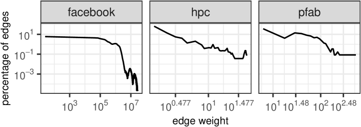
Figure 3: Weight distributions of the four datasets on a log-log scale.

Synthetic Instances

To diversify our test set and to further study the algorithms’ behavior on large instances, we generated synthetic dynamic graphs from RMAT [36] instances, which have also been used to evaluate the static algorithms [25]. Following [25], the initiator matrices for the RMAT generator are $(0.55,0.15,0.15,0.15)$ (rmat_b), $(0.45,0.15,0.15,0.25)$ (rmat_g), and $(0.25,0.25,0.25,0.25)$ (rmat_er), with a number of nodes $n=2^{x}$ and $14\leq x\leq 18$. Whereas each edge is equally likely for the rmat_er (Erdős-Rényi) graphs, rmat_b and rmat_g instances have skewed normal degree distributions, small-world properties, and larger clustering coefficients [37]. The weights follow an exponential distribution with values between $1$ and $500\,000$. We create the dynamic instances as follows: In the first batch, all edges of the static graph are inserted. In every subsequent batch, a fraction $f\in\{0.1,0.3,0.5,0.7,0.9\}$ of edges is updated. If the edge currently has positive weight, its weight is set to zero with probability $p\in\{0.1,0.3\}$, i.e., the edge is deleted. Otherwise we assign a new weight uniformly at random from the weights in the original instance. We obtain $150$ instances altogether, which we group by graph size $n$. Every group contains $30$ instances ($3\times 5\times 2$), each of which has $30$ batches of updates.

On average over all synthetic instances, a batch consists of $17\text{\,}\mathrm{\char 37\relax}$ insertions, $16\text{\,}\mathrm{\char 37\relax}$ deletions and $67\text{\,}\mathrm{\char 37\relax}$ weight changes.

IV-B Setup and Methodology

We implemented the algorithms in C++17 on top of the Algora library. We record the running time and weight of the solution for each batch of updates. When applying a batch, the Algora framework notifies the algorithms of every update individually. The dynamic algorithms dyn-greedy and dyn-kEC immediately update the disjoint matching; the batch-dynamic algorithms batch-greedy, batch-NC, and batch-2apx use these notifications to prepare the batch, i.e., to build up the sets of (nodes incident to) updated edges.

We obtain the number of changes to the coloring over a batch by comparing the coloring before and after the batch. This is done by explicitly storing the state of the coloring before the batch and counting the changes in a separate run, where no running times are measured.

We run our experiments on a machine (A) with two Intel Xeon Gold 6130 CPUs (16 cores each) and $256\text{\,}\mathrm{GB}$ of main memory, and a machine (B) with two Intel Xeon E5-2643 CPUs and $2\times$$750\text{\,}\mathrm{GB}$ of main memory. Machine A was used for all experiments on real-world and synthetic instances, whereas experiments for the split instances were run on machine B. For each experiment, the process was pinned to a NUMA node and its local memory. We focus on the time to obtain a new configuration, i.e., the running time of our algorithms, which are designed to be run on a central server.

To obtain reliable running times, we repeated each experiment three times. For the analysis, we take the median time over each batch for the deterministic algorithms and the arithmetic mean for the randomized algorithms, using different seeds. For the average per-update time $\bar{\tau}_{I}(\mathcal{A})$ of an algorithm $\mathcal{A}$ on an instance $I$, we divide the time per batch by the batch size and take the arithmetic mean over all batches. The average solution weight $\bar{\sigma}_{I}(\mathcal{A})$ is the arithmetic mean over all batches. In case of deterministic algorithms, the average recourse $\bar{o}_{I}(\mathcal{A})$ is defined analogously, whereas for randomized algorithms, we first take the mean recourse per batch over all repetitions and then the mean over these means.

We compare the algorithms relative to each other w.r.t. speedup, solution weight, and recourse. When comparing algorithm $\mathcal{A}$ to a reference algorithm $\mathcal{R}$ for an instance $I$, we obtain (1) the speedup as $\frac{\bar{\tau}_{I}(\mathcal{R})}{\bar{\tau}_{I}(\mathcal{A})}$, (2) the relative solution weight as $\frac{\bar{\sigma}_{I}(\mathcal{A})}{\bar{\sigma}_{I}(\mathcal{R})}$, (3) the relative recourse as $\frac{\bar{o}_{I}(\mathcal{A})}{\bar{o}_{I}(\mathcal{R})}$. To average over a dataset, we always use the geometric mean. Observe that $\mathcal{A}$ is better than $\mathcal{R}$ in terms of speedup and relative solution weight if the value is greater than $1.0$ and vice-versa for recourse.

IV-C Results

We analyze our algorithms first in smaller groups on the set of real-world instances, then consider their performance in terms of running time, solution weight, and recourse on the split and synthetic instances.

Filtering Updates

The update filtering strategy described in Sect. III-E aims at ignoring small updates that are not expected to lead to large changes in the coloring. A preliminary parameter study demonstrated that the decrease in running time due to filtering roughly matched the decrease in solution weight. Combined with post-processing, the speedup was retained, but the solution weight was not impaired. Hence, we present only results for filtering together with post-processing.

Parameters for dyn-greedy

Preliminary results showed that increasing the recursion-depth parameter $\alpha$ beyond $\alpha=1$ yields no significant improvement in the solution weight, but increases the running time. Similarly, when comparing the randomized version of dyn-greedy with $\beta<\max\{k,\Delta\}$ to the deterministic version with $\beta=\max\{k,\Delta\}$, we observed that setting $\beta=1$ yields the best trade-off between running time and solution weight for the randomized algorithm. In the following we thus consider only two versions: a randomized one with $\beta=1$, which is identified by the suffix -r, and a deterministic one without this suffix.

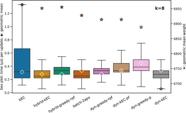
Figure 4: Average per-update times (left axis, boxes and $\blacklozenge$) and weight (right axis, $\star$) for $k=8$ on all real-world instances.

IV-C1 Real-World Instances

Fig. 4 provides an overview over per-update times and solution weights for selected algorithms.

Batch-Dynamic and Static Algorithms

We evaluate the performance of these algorithms relative to each other. Our results confirm the earlier study for the static setting [25] and show that kEC is on average the fastest static algorithm. The same applies to batch-greedy, batch-greedy-l, and batch-NC. For all instances and all $k$, the speedup of NodeCentered and GreedyIt-l is between $0.2$ and $1.5$. However, for each value of $k$, the average speedup across all instances does not exceed $0.9$. GreedyIt is faster than kEC only on the pfab dataset with speedups up to $1.3$, but takes more than twice as long as kEC on the other datasets. Only batch-2apx achieves significant improvements over kEC, with the average speedup over all pfab instances ranging from $1.3$ to $1.7$. On average across all instances, however, kEC remains faster than all batch-dynamic algorithms.

In terms of solution weight, the algorithms differ by no more than $2.5\text{\,}\mathrm{\char 37\relax}$ from the solution weight of kEC. We conclude that among the static and batch-dynamic algorithms, kEC performs best and that batch-2apx is the only batch-dynamic algorithm that is competitive on some datasets. In the following, we hence use kEC as reference for comparisons.

Dynamic Algorithms

We compare dyn-greedy and the randomized dyn-greedy-r to the respective variants with both filtering and post-processing, dyn-greedy-pf and dyn-greedy-rpf. The latter two achieve equal solution weight, which is in all cases at least $98\text{\,}\mathrm{\char 37\relax}$ of the weight achieved by kEC. dyn-greedy-pf is always slower than dyn-greedy-rpf, which achieves speedups between $0.6$ and $3.3$ relative to kEC across all $k$ and instances. The close performance in solution weight of dyn-greedy-pf and dyn-greedy-rpf suggests that the post-processing contributes significantly to the solution weight and can compensate for low-weight solutions produced by the base algorithm.

The randomized dyn-greedy-r cannot match kEC in terms of solution weight. For each $k$, the average solution weight across all instances in FB is below $89\text{\,}\mathrm{\char 37\relax}$ relative to kEC. Also dyn-greedy does not provide an advantage over kEC: it is either significantly slower or its solutions are more than $10\text{\,}\mathrm{\char 37\relax}$ worse. Among the dyn-greedy variants, dyn-greedy-rpf thus offers the best trade-off between solution weight and running time.

The dynamic version of kEC, dyn-kEC, only becomes competitive with kEC when combined with filtering and post-processing. Without either its solutions are about $10\text{\,}\mathrm{\char 37\relax}$ worse than that of kEC on average for each $k$ and it takes up to three times as long as kEC, except for $k\leq 4$ on FB, where the speedup is up to $1.7$. Enabling post-processing (dyn-kEC-p) improves the solution weight slightly, but makes it even slower. The combination with filtering (dyn-kEC-pf) again compensates the loss in running time: dyn-kEC-pf is faster than dyn-kEC overall, but still slower than kEC, however by only $4\text{\,}\mathrm{\char 37\relax}$ on average. Its solution weight is comparable to dyn-greedy-rpf (cf. Fig. 4).

Hybrid Algorithms

kEC and hybrid-kEC perform similar in terms of solution weight, differing in no more than $2\text{\,}\mathrm{\char 37\relax}$ on any instance. hybrid-kEC also tends to be at least as fast as kEC: On average over all $k$ and all instances, it is equally fast on FB, $40\text{\,}\mathrm{\char 37\relax}$ faster on pfab and $8\text{\,}\mathrm{\char 37\relax}$ faster on hpc. Both algorithms do not benefit from post-processing, which increases the running time but not the solution weight.

Hybridizing kEC with dyn-greedy-rpf yields the algorithm hybrid-greedy-rpf, which produces solutions that are for each $k$ on average no more than $1\text{\,}\mathrm{\char 37\relax}$ worse. It is also faster than kEC, with average speedups up to $40\text{\,}\mathrm{\char 37\relax}$.

Summary

kEC is clearly the best static algorithm on the real-world instances, and also superior to all batch-dynamic algorithms except batch-2apx. Among the dynamic algorithms, dyn-greedy-rpf provides the best performance overall, with large speedups and solutions close in weight to those of kEC. hybrid-greedy-rpf and hybrid-kEC are also faster than kEC and have comparable solution weight.

IV-C2 Split Instances

Figure 5: Average per-update times (left axis, boxes and $\blacklozenge$) and weight (right axis, $\star$) for $k=8$ on all split instances.

On the FB/s instances, we see a similar, though not identical picture in comparison to the real-world instances (cf. Fig. 5). One notable difference is that due to the limited maximum edge weight, filtering remains essentially without effect. As the number of updates per sub-batch decreases as the number of sub-batches increases or for a smaller weight limit, the speedup achieved by the dynamic algorithms relative to kEC improves in these cases.

The speedups are more pronounced on average for small $k$. The fastest algorithms across all values of $k$ are dyn-greedy-rp and batch-2apx, both with a mean speedup across all $k$ of $2.5$ and with a maximum speedup over kEC on an instance of $5.1$ and $6.0$, respectively. The hybrid algorithms show a similar performance as kEC with a speedup between $0.85$ and $1.2$.

All algorithms perform similar w.r.t. solution weight, only dyn-greedy-r and dyn-kEC (both without post-processing) fall significantly behind the others with a weight relative to kEC in the ranges $0.70.9$ and $0.50.9$, respectively.

IV-C3 Synthetic Instances

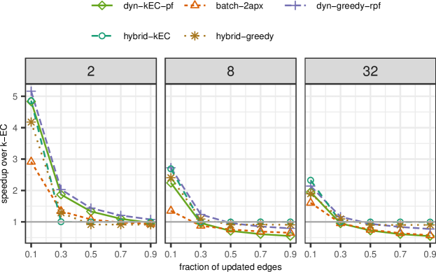
Figure 6: Speedup of (batch-)dynamic algorithms over kEC for $k=2,8,32$ on the synthetic instances, where fraction of updated edges = #updates / m.

kEC is the fastest static algorithm on the synthetic instances. It is also faster than the batch-dynamic algorithms batch-greedy, batch-greedy-l, and batch-NC. batch-2apx is faster than kEC if at most $10\text{\,}\mathrm{\char 37\relax}$ of the edges are updated, and for $k=2$ even if up to half of the edges are updated. The average speedups of batch-2apx over kEC for each $k$ are between $4\text{\,}\mathrm{\char 37\relax}$ and $2.9$.

Fig. 6 shows the speedup of (batch-)dynamic and hybrid algorithms over kEC. The dynamic algorithms are on average faster than kEC if $10\text{\,}\mathrm{\char 37\relax}$ of the edges are updated in a batch. For $k=2$, the dynamic algorithms dyn-greedy-rpf and dyn-kEC-pf achieve a maximum speedup of $5.2$ and $4.0$, respectively, even if $70\text{\,}\mathrm{\char 37\relax}$ of the edges are updated. hybrid-kEC takes on average the same time as kEC unless only $10\text{\,}\mathrm{\char 37\relax}$ of edges are updated. Here, it is significantly faster as it uses the dynamic routine to update the solution. Similarly, hybrid-greedy-rpf is faster if $k=2$ and $10\text{\,}\mathrm{\char 37\relax}$ of edges are updated, but slower if at least half of the edges are updated.

As $k$ increases, the solution weights generally improve relative to kEC and, e.g. for $k=8$, they are already within $6\text{\,}\mathrm{\char 37\relax}$ for all algorithms. The worst case arises for $k=2$ and we discuss it next in more detail: batch-2apx produces solutions that differ from those of kEC by no more than $3\text{\,}\mathrm{\char 37\relax}$ on average. Both hybrid-kEC and hybrid-greedy-rpf match the solution weight of kEC on instances where they mainly employ the static algorithm. However, when only $10\text{\,}\mathrm{\char 37\relax}$ of the edges are updated the solution weight drops off by $10\text{\,}\mathrm{\char 37\relax}$ relative to kEC. This matches the performance of their dynamic counterparts: dyn-kEC-pf and dyn-greedy-rpf yield solutions that are at least $10\text{\,}\mathrm{\char 37\relax}$ lighter than those of kEC when only $10\text{\,}\mathrm{\char 37\relax}$ of edges are updated. With increasing batch size the solution weight improves, but for dyn-kEC-pf does not get within less than $8\text{\,}\mathrm{\char 37\relax}$ of kEC for $k=2$.

In conclusion, while the dynamic algorithms are generally faster than kEC on instances with smaller batch size, the speedup comes at the cost of a somewhat decreased solution weight. For $k=2$, this decrease can be quite significant, but it improves for larger $k$. batch-2apx produces high-weight solutions even for $k=2$, which are within $3\text{\,}\mathrm{\char 37\relax}$ of kEC’s. Thus, batch-2apx is the recommended choice for small $k$, whereas hybrid-kEC and hybrid-greedy-rpf are faster for larger $k$ without sacrificing solution weight.

IV-C4 Recourse

We compare the best algorithms from the previous sections. As the static algorithms differ in recourse by no more than $2\text{\,}\mathrm{\char 37\relax}$, we use kEC as reference.

Real-World Instances

dyn-greedy-rpf and batch-2apx have similar recourse on FB and hpc, which is between $56\text{\,}\mathrm{\char 37\relax}$ and $69\text{\,}\mathrm{\char 37\relax}$ of kEC’s. On pfab, batch-2apx is slightly better than dyn-greedy-rpf and clearly better than kEC. dyn-kEC-pf performs similarly well as dyn-greedy-rpf on hpc and pfab, and even better on FB with a recourse of at most $39\text{\,}\mathrm{\char 37\relax}$ relative to kEC.

The recourse of the hybrid algorithms tends to be between kEC and their dynamic subroutine. hybrid-kEC performs equal to kEC on FB, better on hpc, but worse on pfab. hybrid-greedy-rpf has lower recourse than kEC on all instances and matches that of dyn-greedy-rpf on pfab.

Synthetic Instances

We expect the recourse of the dynamic and hybrid algorithms to be less than that of kEC for small batch sizes. The results on the synthetic instances confirm this. dyn-greedy-rpf, dyn-kEC-pf, and batch-2apx show similar results in terms of recourse: for $k=2$ the recourse ranges between $50\text{\,}\mathrm{\char 37\relax}$ and $95\text{\,}\mathrm{\char 37\relax}$ relative to kEC and between $22\text{\,}\mathrm{\char 37\relax}$ and $36\text{\,}\mathrm{\char 37\relax}$ for $k=32$. As expected, the recourse increases with the batch size. Surprisingly on first sight, the recourse relative to kEC decreases as $k$ increases. However, for larger $k$ more edges are colored and, thus, a larger percentage of edges keep their color during an update. The hybrid algorithms hybrid-kEC and hybrid-greedy-rpf have the same recourse as kEC if at least half of the edges are updated in a batch. If only $10\text{\,}\mathrm{\char 37\relax}$ of edges are updated, the recourse is similar to their dynamic counterparts. This behavior reflects the above discussion of running times and solution weights.

Split Instances

We observe a similar reduction in recourse for small batches on the split instances FB/s. hybrid-kEC and hybrid-greedy-rp showed the same performance w.r.t. running time and solution weight, and they also produce the same recourse as kEC, regardless of batch size. The dynamic algorithms’ recourse is on average at least $20\text{\,}\mathrm{\char 37\relax}$ lower than that of kEC. Post-processing has a significant impact on recourse: for dyn-greedy-rp has average recourse up to twice that of dyn-greedy-r. A similar trend can be seen for dyn-kEC-p compared to dyn-kEC, but the effect is not as pronounced. Filtering, on the other hand, has no significant impact on the recourse, which also matches our observations w.r.t. running time and solution weight. In general, the recourse relative to kEC increases for dynamic algorithms as the batches become larger. For $k=2$ dyn-greedy-rp produces an average recourse between $51\text{\,}\mathrm{\char 37\relax}$ and $73\text{\,}\mathrm{\char 37\relax}$ and $44\text{\,}\mathrm{\char 37\relax}$ to $74\text{\,}\mathrm{\char 37\relax}$ for $k=32$. dyn-kEC-p, dyn-greedy-rp and batch-2apx have a recourse roughly equal to dyn-greedy-rp.

Summary

The (batch-) dynamic and hybrid algorithms generally have a smaller recourse than the static algorithms, which leads to fewer changes in the network configuration. On instances where the hybrid algorithms mainly use the static kEC, they have no advantage in terms of recourse.

IV-C5 Summary of Experiments

Our results show that dynamic algorithms are particularly good on instances with smaller batches, while static algorithms perform well on large batches. This suggests the following recommendations: (1) When dealing with small batches and small numbers of matchings, i.e., frequent reconfigurations of the network and a small number of switches, batch-2apx exhibits the best trade-off between running time and solution weight. (2) For a larger number of matchings, the dynamic algorithms dyn-greedy-rpf and dyn-kEC-pf provide faster running times and high-weight solutions. (3) When dealing with large batches, e.g. if the intervals between reconfigurations are longer, the hybrid algorithms hybrid-kEC and hybrid-greedy-rpf provide the best performance if running time, solution weight, and recourse are considered. They are also well-suited for other situations and thus are a very good general-purpose choice. (4) If the solution weight has the top priority and sacrifices w.r.t. running time and recourse are acceptable, the best choice is kEC. Generally, the dynamic and hybrid algorithms have a lower recourse than the static algorithms, with dyn-kEC-pf giving recourse as low as $30\text{\,}\mathrm{\char 37\relax}$ relative to kEC. Note that reduced recourse implies less reconfiguration cost in the optical network and, thus, less overhead.

V Conclusion

To improve the performance of emerging reconfigurable datacenter networks, we studied efficient algorithms to maximize the amount of traffic which can be offloaded to the optical topology in a demand-aware manner. In particular, we presented several dynamic algorithms which exploit the temporal structure of workloads, by computing the disjoint matchings offered by optical switches in an adaptive manner.

Our work opens several interesting avenues for future research. In particular, we have so far focused on algorithms running on a centralized controller, which matches the predominant architectural datacenter network model today [38, 27, 31]. Still, it would be interesting to explore distributed versions of our algorithms: emerging reconfigurable datacenter architectures support a distributed control, e.g., performed directly on the switches. Furthermore, we have so far focused on online algorithms which do not require any knowledge of future traffic demands. This is attractive, as the predictability of such traffic demands is application-specific. Nevertheless, it would be interesting to explore how a dynamic scheduler can benefit from headroom, as it may be available for repetitive applications (e.g., related to learning): such knowledge may be exploited to pre-compute solutions dynamically to some extent and hence to further improve the algorithms. Our algorithms may also be adapted to the related problem of scheduling connections in satellite-based communication networks, where colors correspond to time slots [28]. The problem differs in that the matchings are unweighted and bounded in cardinality.

References

- [1] Y. Li, R. Miao, H. H. Liu, Y. Zhuang, F. Feng, L. Tang, Z. Cao, M. Zhang, F. Kelly, M. Alizadeh et al., “Hpcc: High precision congestion control,” in Proceedings of the ACM Special Interest Group on Data Communication, 2019, pp. 44–58.
- [2] M. Khani, M. Ghobadi, M. Alizadeh, Z. Zhu, M. Glick, K. Bergman, A. Vahdat, B. Klenk, and E. Ebrahimi, “SiP-ML: high-bandwidth optical network interconnects for machine learning training,” in Proceedings of the ACM SIGCOMM, 2021, pp. 657–675.
- [3] J. C. Mogul and L. Popa, “What we talk about when we talk about cloud network performance,” ACM SIGCOMM Computer Communication Review, vol. 42, no. 5, pp. 44–48, 2012.
- [4] X. Zhou, Z. Zhang, Y. Zhu, Y. Li, S. Kumar, A. Vahdat, B. Y. Zhao, and H. Zheng, “Mirror mirror on the ceiling: Flexible wireless links for data centers,” ACM SIGCOMM Computer Communication Review, vol. 42, no. 4, pp. 443–454, 2012.
- [5] S. Kandula, J. Padhye, and V. Bahl, “Flyways to de-congest data center networks,” 2009.
- [6] N. Hamedazimi, Z. Qazi, H. Gupta, V. Sekar, S. R. Das, J. P. Longtin, H. Shah, and A. Tanwer, “Firefly: A reconfigurable wireless data center fabric using free-space optics,” in Proceedings of the ACM SIGCOMM, 2014, pp. 319–330.
- [7] K. Chen, A. Singla, A. Singh, K. Ramachandran, L. Xu, Y. Zhang, X. Wen, and Y. Chen, “Osa: An optical switching architecture for data center networks with unprecedented flexibility,” IEEE/ACM Transactions on Networking, vol. 22, no. 2, pp. 498–511, April 2014.
- [8] M. Ghobadi, R. Mahajan, A. Phanishayee, N. R. Devanur, J. Kulkarni, G. Ranade, P. Blanche, H. Rastegarfar, M. Glick, and D. C. Kilper, “ProjecToR: Agile reconfigurable data center interconnect,” in Proceedings of the ACM SIGCOMM, 2016, pp. 216–229.
- [9] M. Hampson, “Reconfigurable optical networks will move supercomputerdata 100x faster,”,” IEEE Spectrum, 2021.
- [10] F. Douglis, S. Robertson, E. Van den Berg, J. Micallef, M. Pucci, A. Aiken, K. Bergman, M. Hattink, and M. Seok, “Fleet—fast lanes for expedited execution at 10 terabits: Program overview,” IEEE Internet Computing, vol. 25, no. 3, pp. 79–87, 2021.
- [11] C. Avin, K. Mondal, and S. Schmid, “Demand-aware network designs of bounded degree,” Distributed Computing, vol. 33, no. 3, pp. 311–325, 2020.
- [12] M. Y. Teh, Z. Wu, and K. Bergman, “Flexspander: augmenting expander networks in high-performance systems with optical bandwidth steering,” Journal of Optical Communications and Networking, vol. 12, no. 4, pp. B44–B54, 2020.
- [13] C. Griner, J. Zerwas, A. Blenk, S. Schmid, M. Ghobadi, and C. Avin, “Cerberus: The power of choices in datacenter topology design (a throughput perspective),” in Proc. ACM SIGMETRICS, 2022.
- [14] C. Avin and S. Schmid, “Toward demand-aware networking: A theory for self-adjusting networks,” in ACM SIGCOMM Computer Communication Review (CCR), 2018.
- [15] C. Avin, M. Ghobadi, C. Griner, and S. Schmid, “On the complexity of traffic traces and implications,” in Proc. ACM SIGMETRICS, 2020.
- [16] A. Roy, H. Zeng, J. Bagga, G. Porter, and A. C. Snoeren, “Inside the social network’s (datacenter) network,” Proceedings of the ACM SIGCOMM, 2015.
- [17] S. Kandula, S. Sengupta, A. Greenberg, P. Patel, and R. Chaiken, “The nature of data center traffic: measurements & analysis,” in Proceedings of the ACM Internet Measurement, 2009, pp. 202–208.
- [18] W. M. Mellette, R. McGuinness, A. Roy, A. Forencich, G. Papen, A. C. Snoeren, and G. Porter, “Rotornet: A scalable, low-complexity, optical datacenter network,” in Proceedings of the ACM SIGCOMM, 2017, pp. 267–280.
- [19] J. Kulkarni, S. Schmid, and P. Schmidt, “Scheduling opportunistic links in two-tiered reconfigurable datacenters,” in 33rd ACM Symposium on Parallelism in Algorithms and Architectures (SPAA), 2021.
- [20] N. Farrington, G. Porter, S. Radhakrishnan, H. H. Bazzaz, V. Subramanya, Y. Fainman, G. Papen, and A. Vahdat, “Helios: a hybrid electrical/optical switch architecture for modular data centers,” ACM SIGCOMM Computer Communication Review, vol. 41, no. 4, pp. 339–350, 2011.
- [21] A. Singla, A. Singh, K. Ramachandran, L. Xu, and Y. Zhang, “Proteus: a topology malleable data center network,” in Proceedings of the ACM Workshop on Hot Topics in Networks, 2010, pp. 1–6.
- [22] G. Wang, D. G. Andersen, M. Kaminsky, K. Papagiannaki, T. E. Ng, M. Kozuch, and M. Ryan, “c-through: Part-time optics in data centers,” in Proceedings of the ACM SIGCOMM, 2010, pp. 327–338.
- [23] S. B. Venkatakrishnan, M. Alizadeh, and P. Viswanath, “Costly circuits, submodular schedules and approximate carathéodory theorems,” Queueing Systems, vol. 88, no. 3-4, pp. 311–347, 2018.
- [24] C. Avin and S. Schmid, “Renets: Statically-optimal demand-aware networks,” in Proc. SIAM Symposium on Algorithmic Principles of Computer Systems (APOCS), 2021.
- [25] K. Hanauer, M. Henzinger, S. Schmid, and J. Trummer, “Fast and heavy disjoint weighted matchings for demand-aware datacenter topologies,” in IEEE Conference on Computer Communications, INFOCOM, 2022.
- [26] H. Ballani, P. Costa, R. Behrendt, D. Cletheroe, I. Haller, K. Jozwik, F. Karinou, S. Lange, K. Shi, B. Thomsen, and H. Williams, “Sirius: A flat datacenter network with nanosecond optical switching,” in Proceedings of the ACM SIGCOMM, 2020, pp. 782–797.
- [27] M. Zhang, J. Zhang, R. Wang, R. Govindan, J. C. Mogul, and A. Vahdat, “Gemini: Practical reconfigurable datacenter networks with topology and traffic engineering,” CoRR, 2021.
- [28] U. Feige, E. Ofek, and U. Wieder, “Approximating maximum edge coloring in multigraphs,” in International Workshop on Approximation Algorithms for Combinatorial Optimization, 2002, pp. 108–121.
- [29] J. Zerwas, C. Gyorgyi, A. Blenk, S. Schmid, and C. Avin, “Duo: A high-throughput reconfigurable datacenter network using local routing and control,” in ACM SIGMETRICS, 2023.
- [30] V. Addanki, C. Avin, and S. Schmid, “Mars: Near-optimal throughput with shallow buffers in reconfigurable datacenter networks,” in ACM SIGMETRICS, 2023.
- [31] M. N. Hall, K.-T. Foerster, S. Schmid, and R. Durairajan, “A survey of reconfigurable optical networks,” in Optical Switching and Networking (OSN), Elsevier, 2021.
- [32] K. Hanauer, M. Henzinger, and C. Schulz, “Recent advances in fully dynamic graph algorithms - A quick reference guide,” ACM J. Exp. Algorithmics, vol. 27, pp. 1.11:1–1.11:45, 2022.
- [33] M. Bienkowski, D. Fuchssteiner, J. Marcinkowski, and S. Schmid, “Online dynamic b-matching: With applications to reconfigurable datacenter networks,” SIGMETRICS Perform. Evaluation Rev., vol. 48, no. 3, pp. 99–108, 2020.
- [34] J. Misra and D. Gries, “A constructive proof of Vizing’s theorem,” Inf. Process. Lett., vol. 41, no. 3, pp. 131–133, 1992.
- [35] M. Alizadeh, S. Yang, M. Sharif, S. Katti, N. McKeown, B. Prabhakar, and S. Shenker, “pfabric: minimal near-optimal datacenter transport,” Proceedings of the ACM SIGCOMM, 2013.
- [36] D. Chakrabarti, Y. Zhan, and C. Faloutsos, “R-MAT: A recursive model for graph mining,” in Proceedings of the Fourth SIAM International Conference on Data Mining, 2004, pp. 442–446.
- [37] M. Halappanavar, J. Feo, O. Villa, A. Tumeo, and A. Pothen, “Approximate weighted matching on emerging manycore and multithreaded architectures,” Int. J. High Perform. Comput. Appl., vol. 26, no. 4, pp. 413–430, 2012.
- [38] A. Singh, J. Ong, A. Agarwal, G. Anderson, A. Armistead, R. Bannon, S. Boving, G. Desai, B. Felderman, P. Germano et al., “Jupiter rising: A decade of clos topologies and centralized control in google’s datacenter network,” ACM SIGCOMM computer communication review, vol. 45, no. 4, pp. 183–197, 2015.
- [39] https://doi.org/10.5281/zenodo.7535351.