The Commutativity Quotients
of Concurrent Objects

Abstract

Concurrent objects form the foundation of many applications that exploit multicore architectures. Reasoning about the fine-grained complexities (interleavings, invariants, etc.) of those data structures, however, is notoriously difficult. Formal proof methodologies for arguing about the correctness—i.e.,  linearizability—of these data structures are still somewhat disconnected from the intuitive correctness arguments. Intuitions are often about a few canonical executions, possibly with few threads, whereas formal proofs would often use generic but complex arguments about arbitrary interleavings over unboundedly many threads.

As a way to bring formal proofs closer to intuitive arguments, we introduce a new methodology for characterizing the interleavings of concurrent objects, based on their commutativity quotient. This quotient represents every interleaving up to reordering of commutative steps and, when chosen carefully, admits simple abstractions in the form of regular or context-free languages that enable simple proofs of linearizability. We demonstrate these facts on a large class of lock-free data structures and the infamously difficult Herlihy-Wing Queue. We automate the discovery of these execution quotients and show it can be automatically done for challenging data-structures such as Treiber’s stack, Michael/Scott Queue, and a concurrent Set implemented as a linked list.

1 Introduction

Efficient multithreaded programs typically rely on optimized implementations of common abstract data types (adts) like stacks, queues, and sets, whose operations execute in parallel across processor cores to maximize efficiency. Programming these so-called concurrent objects is tricky though. Synchronization between operations must be minimized to increase throughput [15, 33]. Yet this minimal amount of synchronization must also be adequate to ensure that operations behave as if they were executed atomically, one after the other, so that client programs can rely on their (sequential) adt specification; this de-facto correctness criterion is known as linearizability [17]. These opposing requirements, along with the general challenge in reasoning about thread interleavings, make concurrent data structures a ripe source of insidious programming errors [30].

Proving that concurrent objects are correct is a very challenging problem that has been addressed in many works (see Section 8 for a discussion). Despite this progress, there is still somewhat of a disconnect between existing formal proofs and the intuitive arguments for correctness used by algorithm designers. Existing formal proof methodologies generally rely on inductive invariants or assertions about arbitrary interleavings of unboundedly-many steps, which are hard to devise and manipulate. On the other hand, algorithm designers (e.g., researchers defining new concurrent objects) argue about correctness by considering some number of “scenarios”, i.e., interesting ways of interleaving steps of different operations, and showing for instance, that each one satisfies some suitable invariant (which is not necessarily inductive). However, these proof arguments are most often informal and sometimes prone to errors.

Reasoning about Execution Quotients. In this work, we propose a new proof methodology that is based on formal arguments while keeping the intuition of scenario-based reasoning. This methodology relies on a reduction to reasoning about a subset of representative interleavings, which cover the whole space of interleavings modulo repeatedly swapping adjacent commutative steps. The latter corresponds to the standard equivalence up to commutativity between the executions of an object (Mazurkiewicz traces [29]).

Reductions based on commutativity arguments have been formalized in previous work, e.g.,  Lipton’s reduction theory [28], QED [8], CIVL [12], and they generally focus on identifying atomic sections, i.e.,  sequences of statements in a single thread that can be assumed to execute without interruption (without sacrificing completeness). Relying on atomic sections for reducing the space of interleavings has its limitations, especially in the context of concurrent objects. These objects rely on intricate algorithms where almost every step is an access to the shared memory that does not commute with respect to other steps.

Our reduction argument reasons about a quotient of the set of object executions, which is a subset of executions that contains a representative from each equivalence class. In general, an execution of an object interleaves an unbounded number of invocations to the object’s methods, each from a different thread. It can be seen as a word over an infinite alphabet, each symbol of the alphabet representing a statement in the object’s source code and the thread executing that statement. We show that when abstracting away thread ids from executions, carefully chosen quotients become regular or context-free languages. This is not true for any quotient since representatives of equivalence classes can be chosen in an adversarial manner to make the language more complex. Reasoning about the correctness of executions in such quotients is much simpler than reasoning about the entire set of executions of an object.

Layer Quotients. For lock-free objects, we define a particular class of layer quotients whose executions can be decomposed into a sequence of layers representing interleavings of unboundedly many threads but with a “regular” shape.

The shape of layers relies on the fact that methods of a lock-free object are typically implemented as an infinite while(true) loop where each iteration tries to update the state according to the specification and if it fails, i.e., it observes interference from conflicting updates in other threads, then a new iteration is started afresh. A layer is defined by an interleaving of control-flow paths representing (partial) loop iterations from different threads where at most one so-called write-path contains some successful atomic read-write to update the object state. The control-flow paths without a successful atomic read-write, called local paths, are typically iterations that fail their atomic read-write because of the interference caused by the successful atomic read-write in the same layer. Such paths can be replicated an unbounded number of times in different threads. Each layer summarizes at most one iteration with a successful atomic read-write and its impact on the “failed” iterations of other threads. Intuitively, a layer can be abstractly seen as an expression from a context-free language $a_{1}^{n}\cdot b\cdot a_{2}^{n}$ where $a_{1}\cdot a_{2}$ forms a local path and $b$ is an iteration that contains a successful atomic read-write, or as a regular language expression $a^{*}$ if it contains no successful atomic read-write. The exponents in both expressions indicate the unbounded replication of local paths ($n$ is not fixed; it ensures prefix/suffix balancing). Note that these are simplified examples used only for intuition.

Reasoning about the linearizability of executions in the layer quotient is simpler compared to arbitrary executions because the correspondence between such executions and the so-called linearizations is quite straightforward. We recall that linearizability demands that every method invocation in an execution appears to take effect instantaneously at some point between the invocation and the response. The order in which invocations take effect defines a linearization of the execution, and proving linearizability boils down to defining a correspondence between executions and linearizations thereof and showing that the linearizations satisfy the intended specification (adt). Each layer corresponds to linearizing a single effectful invocation, e.g.,  adding an element to a stack, or an arbitrary number of read-only invocations, i.e.,  pops that return that the stack is empty.

Showing that layer expressions are abstractions of quotients, i.e.,  they include a representative of each equivalence class, can be reduced to reasoning about two-threaded programs, which turns out to be sufficient for characterizing equivalence between traces of unboundedly many threads. Essentially, it requires that every local control-flow path, i.e.,  composed only of local steps, can be assumed to interleave with at most one other write path, i.e.,  containing an atomic read-write, and every write path can be assumed to execute in isolation. We show that several canonical concurrent objects, e.g.,  Treiber’s Stack [45], Michael/Scott queue [31], Scherer/Lea/Scott synchronous reservation queue [43], and a linked-list Set [36] admit layer expression abstractions of their quotients.

Finally we describe how layer expressions represented as finite-state automata can be automatically derived from object implementations. The automata are defined by a number of states that, roughly, represent pre-conditions of layers, and a number of layer-labeled transitions. Although they represent interleavings of unboundedly-many threads, these automata are computed by reasoning about programs with at most two threads. As in the case of quotient completeness, this is sound because failed iterations do not cause any interference and one can reason about each such iteration in an independent manner. We implemented a prototype tool called Cion that performs this algorithm on object implementations. We applied Cion to canonical examples including Treiber’s Stack, the Michael/Scott Queue, and a concurrent Set implemented as a linked list and find that layer expressions for these objects can be discovered in a few minutes.

Beyond Layer Quotients. While the idea of reasoning about execution quotients is generic, identifying precise limits for the applicability of the particular class of layer quotients is hard in general. However, there exist objects such as the Herlihy and Wing queue [17], which do not admit quotients defined as sequences of layers. This queue stores the elements into an infinite array items. An enqueue adds a value in two steps, first reserving a slot in the array and then, putting a value in that slot. A dequeue traverses the array multiple times looking for a slot containing an item to atomically dequeue. We show that this object admits a quotient where each array traversal in the dequeue can be considered to be an atomic section, and writes to an array slot in enqueues before a successful dequeue traversal (that finds an item to dequeue) are ordered according to the array slots they write to. The traces in such a quotient can be shown linearizable by taking every second write in an enqueue and every successful dequeue iteration to be their linearization points. This is an important simplification, because for arbitrary traces, linearization points depend on the future and can not be associated to fixed statements; see e.g.,  Schellhorn et al. [42].

Contributions. In summary, this work makes the following contributions:

• We introduce a new formal reasoning methodology for verifying concurrent objects that relies on execution quotients.

• We define the concept of layer expression abstractions of quotients and demonstrate their applicability in the context of lock-free objects.

• We establish a methodology for proving soundness of layer quotients which reduces to reasoning about two-threaded programs.

• We define an automata-based representation of layer quotients and an algorithm for computing such representations.

• We implement this algorithm and evaluate it on several canonical examples.

• We show a reduction to execution quotients which simplifies reasoning about the Herlihy and Wing queue even if they fall out of the layer quotient class.

We plan to make our implementation Cion publicly available. Benchmark sources and the tool output in LaTeX format are provided as supplementary materials.

2 Overview

Figure 1 lists a concurrent counter with two methods for incrementing and decrementing the counter. Both methods return the value of the counter before modifying it, and the counter is decremented only if it is strictly positive.

⬇

1int increment() {

2 while (true) {

3 int c = ctr;

4 if (CAS(ctr, c, c+1))

5 return c;

6 }

7}

⬇

8int decrement() {

9 while (true) {

10 int c = ctr;

11 if ( c == 0 )

12 return 0;

13 if (CAS(ctr, c, c-1))

14 return c;

15 }

16}

Figure 1: A concurrent counter.

Each method consists of a retry-loop that reads the shared variable ctr representing the value of the counter and tries to update it using a Compare-And-Swap (CAS) statement (unless ctr is zero and the counter cannot be decremented). A CAS statement atomically tests whether ctr has the value specified by the second argument and if this is the case, then it assigns to ctr the value specified by the third argument (if the test fails, then CAS has no effect). The return value of CAS represents the truth value of the equality test. If the CAS is unsuccessful, i.e.,  it returns false, then the method retries executing the same steps in another iteration.

The executions of the concurrent counter are interleavings of an arbitrary number of increment or decrement invocations from an arbitrary number of threads. Each invocation executes a number of retry-loop iterations until reaching the return. An iteration corresponds to a control-flow path that starts at the beginning of the loop and ends with a return or goes back to the beginning of the loop. For instance, the increment method consists of two possible iterations:

1. $\texttt{c}=\texttt{ctr}\mathchar 24635\relax\;\texttt{CAS(ctr, c, c+1)}\mathchar 24635\relax\;\texttt{return c}$
2. $\texttt{c}=\texttt{ctr}\mathchar 24635\relax\;\texttt{assume(ctr != c)}$

The first iteration is called successful because it contains a successful CAS, and the unsuccessful CAS in the second iteration is written as an assume that blocks if the condition is not satisfied.

An invocation can execute more than one iteration if the ctr variable is modified by another thread in between reading it at line 3 or 10 and executing the CAS statement at line 4 or 13, respectively. For instance, Figure 2 pictures an execution with three increment invocations that execute between one and three retry-loop iterations. The first iteration of threads 2 and 3 contains unsuccessful CASs because thread 1 executed a successful CAS and modified ctr, and these invocations must retry and execute more iterations.

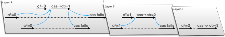
Figure 2: Layer quotient of an increment-only execution with three threads whose actions are aligned horizontally. For readability, we rename the local variable c in thread $i$ to $\texttt{c}^{i}$. The curved blue arrows depict data-flow dependencies between reads/writes of ctr.

2.1 Layer Execution Quotients

Fig. 2 is only one execution. There are infinitely more executions and, even with bounded threads, there are exponentially many interleavings. On the other hand, pragmatic informal correctness arguments are made by appealing to a handful of execution patterns. The key idea of this paper is to bridge this gap with the notion of the quotient of all executions of a concurrent object denoted $\langle\!\lfloor O\rfloor\!\rangle$. This quotient reduces reasoning to representative, canonical traces, with all other traces equivalent to at least one representative trace in the quotient. The trace in Fig. 2 is one such representative trace and is already in a canonical form. We call this canonical form a sequence of layers where each layer groups together the retry-loop iterations that interact with each other. For instance, the execution in Fig. 2 can be seen as a sequence of three layers—as depicted with stacked parallelograms—each layer including an iteration with a successful CAS from threads 1, 2, and 3, respectively (and iterations with unsuccessful CASs from other threads). Each individual layer is a sequence of statements of the form $[\texttt{c:=ctr}^{n}\cdot(\texttt{c:=ctr;cas(ctr,c,c+1)/true})\cdot\texttt{cas/false}^{n}]$ where $n$ threads begin to read ctr, then a single different thread performs its complete write path (which is atomic w.r.t. concurrent reads), and then all $n$ threads fail their CAS instructions. In this way, each layer corresponds to linearizing a single effectful invocation, i.e.,  an increment invocation or a decrement invocation when the counter is non-zero, or an arbitrary number of read-only invocations, i.e.,  decrement invocations when the counter is zero. The overall layer quotient of the Counter object is all sequential compositions of similarly defined layers.

We define quotients in a general sense in Sec. 4. First, semantically, a quotient $\langle\!\lfloor O\rfloor\!\rangle$ is a subset of the executions that is complete in the sense that all other executions can be obtained through commutative swappings from some element of $\langle\!\lfloor O\rfloor\!\rangle$, and no two elements of $\langle\!\lfloor O\rfloor\!\rangle$ are equivalent.

2.2 Layer expression abstractions of object quotients

Describing a quotient set presents another challenge and, in Sec. 4, we introduce a quotient expression language using a mixture of regular expressions and context-free grammars, along with its interpretation as sets of traces. The expression $[\texttt{c:=ctr}^{n}\cdot(\texttt{c:=ctr;cas(ctr,c,c+1)/true})\cdot\texttt{cas/false}^{n}]^{*}$ is an abstraction of the quotient of the Counter, when considering only increment operations: from any execution of the Counter one can find another execution that is in the interpretation of this expression. Such an expression is interpreted as a set of traces where, for any $n$, thread ids are associated with individual statements. To avoid redundancy, the interpretation assumes some canonical ordering on thread ids. Below we will extend the expression slightly to also cover concurrent decrement operations but let us first consider unboundedly many increments.

Unbounded increments. Each layer contains a single retry-loop iteration with a successful CAS interleaved with an arbitrary number of retry-loop iterations with unsuccessful CASs (from other threads). Every unsuccessful iteration is required to fail because of the interference caused by the successful CAS in the same layer, i.e.,  it must form a data dependency cycle with the latter by reading the value of ctr before and after the successful CAS (the second read corresponds to the CAS test). Note that the lack of a data dependency cycle would imply that the two iterations can be reordered so that one completes before the other.

The expression defined above is an abstraction of the quotient because every execution is equivalent (up to reordering of commutative steps) to an execution in the interpretation of this expression, in which layers are executed in isolation one after another. The execution in Figure 2 is an execution in the interpretation that is also directly in a quotient $\langle\!\lfloor O\rfloor\!\rangle$ because all the actions in layer $i$ are executed before all the actions in layer $j>i$ and the failing read-only threads are put in a canonical form within each layer. What remains is to show that all other traces, beyond the canonical traces such as the one depicted in Figure 2 are equivalent, via commutative re-ordering, to some trace in the quotient.

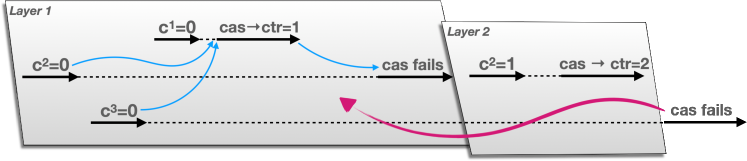
Figure 3: An increment-only execution for which there is an equivalent representative execution (as suggested by the large wavy arrow) that is in the layer quotient.

To explain the equivalence between arbitrary interleavings of increment invocations and representative executions in quotient $\langle\!\lfloor O\rfloor\!\rangle$, we consider the execution pictured in Figure 3. This execution is not in $\langle\!\lfloor O\rfloor\!\rangle$ because the unsuccessful iteration of thread 3 is interleaved with two successful CASs: it reads ctr before the first successful CAS (in thread 1) and after the second successful CAS (in thread 2). Yet, as explained above, a layer interleaves an unsuccessful iteration with a single successful CAS.

However, the second read of ctr, corresponding to the unsuccessful CAS in thread 3, is enabled even if executed earlier just after the first successful CAS. Moreover, since retry-loop iterations are “forgetful”, i.e.,  there is no flow of data from one iteration to the next (the value of ctr is read anew in the next iteration), executing the unsuccessful CAS earlier would not affect the future behavior of this thread (and any other thread because it is a read) even if this reordering makes this unsuccessful CAS read a different value of ctr (value 1 instead of 2). This reasoning extends even when the iteration of thread 3 is interleaved with more than two other iterations.

The case of increment-only executions is simpler because it does not include the so-called ABA scenarios in which ctr is changed to a new value and later restored to a previous value. Every successful CAS will write a new value to ctr and will make all the other invocations that read ctr just before to restart.

Figure 4: An execution where the second thread executes a decrement, which is equivalent to the representative execution suggested by the wavy arrow.

Increment and Decrement Executions. Interleavings of increment and decrement invocations can exhibit the ABA scenario described above, as exemplified in Figure 4. The value 0 read by thread 3 before the first successful CAS is restored by the second successful CAS (performed in a decrement invocation). This execution is not a representative execution in $\langle\!\lfloor O\rfloor\!\rangle$ because the successful retry-loop iteration in thread 3 interleaves with other two successful iterations while in $\langle\!\lfloor O\rfloor\!\rangle$ executions, every successful iteration is executed in isolation w.r.t. other successful iterations. However, the equality test in the successful CAS of thread 3 (ctr == 0) is enough to conclude that the previous read can be commuted to the right and just before the CAS. This allows to group together the actions of the third layer and obtain a representative execution from $\langle\!\lfloor O\rfloor\!\rangle$, extended to include decrements. To this end, we introduce decrement layers of the form $[(\texttt{c:=ctr}_{inc}^{n}\cdot\texttt{c:=ctr}_{dec}^{m})\cdot\texttt{c:=ctr;cas(ctr,c,c-1)/true}\cdot(\texttt{cas/false}_{dec}^{m}\cdot\texttt{cas/false}_{inc}^{n})$. In this expression, $n$ concurrent increment threads and $m$ concurrent decrement threads interleave with a single successful decrement thread (we also subscripted with $inc/dec$ to indicate where the action came from.). All unsuccessful threads’ operations commute with each other and are put in a canonical form (later the interpretation of $a^{n}$ will order $a$’s according to thread ids). We similarly augment the increment layers with concurrent decrement threads.

Decrement invocations can also be formed exclusively of read-only iterations when they observe that ctr is 0. The last iteration in such invocations returns 0 and performs no write to the shared memory. Such loop iterations that read the value of ctr at the same time (after the same number of successful CASs) are grouped in a layer as well. They can be assumed to execute in isolation because they execute a single memory access.

To prove that the layer expression is an abstraction of the quotient, somewhat surprisingly, it is sufficient to reason about interleavings of a two-threaded program where one thread performs a single iteration and the other thread performs a sequence of successful iterations (where the CAS succeeds). This holds because unsuccessful iterations do not affect the computation of other threads.

Layer expression abstraction Overall, a quotient of the counter contains sequences of layers as described above. The order in which layers can occur in an execution can be constrained using regular expressions or equivalently, automata representations as shown in Fig. 5. In this layer automaton, states are properties of the shared memory that identify preconditions enabling shared-memory writes (successful CASs), and transitions represent layers (to be executed in isolation).

This automaton consists of two states depicted in dark gray, distinguishing shared-memory configurations where the precondition of a successful CAS in decrement invocations (ctr $>$ 0) holds. The self-loop on the initial state represents a layer (Layer 1) formed of an arbitrary number of decrement iterations returning value 0, executed by possibly different threads. “dec:10-11-ret(0)” refers to the control-flow path of decrement from Line 10 to Line 11 to return. (In our formalization we will summarize paths using Kleene Algebra with Test (KAT) expressions.) Layer 2 occurs on the outgoing transition from the initial state and this layer is formed from a successful increment iteration interleaved with an arbitrary number of unsuccessful increment iterations executed by different threads (when ctr equals 0 all decrement retry-loop iterations reach the return statement). Iterations are represented as control-flow paths in the code of the methods. inc:3-5-cas()/true summarizes the single successful write path in the layer: an increment control-flow path that begins on Line 3, proceeds to the CAS, succeeds the CAS and returns. The final expression in Layer 2 summarizes an arbitrary number of threads failing the test on Line 4 (due to the successful write path), and loop back to Line 3. The outgoing transitions from the second state represent layers containing a successful increment (Layer 3) or decrement iteration (Layer 4), each interleaved with an arbitrary number of unsuccessful increment or decrement iterations. Finally, the transition from ctr$>$0 to ctr=0 involves the same Layer 4, despite landing in a new automaton state.

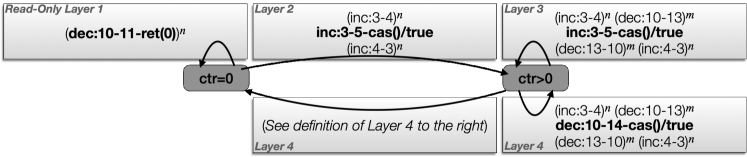
Figure 5: An automaton representation of layer-serialized executions of the counter.

3 Preliminaries

We model programs using Kleene Algebra with Tests [22] (KAT) a formalism similar to symbolic automata [14, 7], but having convenient algebraic properties (e.g.,  composition, iteration, tests) that simplify our presentation. Our KATs represent traces as combinations of conditionals (tests) and statements (actions).

Definition 1

[Kleene Algebra with Tests] A KAT $\mathcal{K}$ is a two-sorted structure $(\Sigma,\mathcal{B},+,\;\cdot\;,*,\overline{\;},0,1)$, where $(\Sigma,+,\;\cdot\;,*,0,1)$ is a Kleene algebra, $(\mathcal{B},+,\;\cdot\;,\overline{\;},0,1)$ is a Boolean algebra, and the latter is a subalgebra of the former. There are two sets of symbols: A for primitive actions, and B for primitive tests. The grammar of boolean test expressions is $BExp::=b\in\textsf{B}\mid b\cdot b\mid b+b\mid\overline{b}\mid 0\mid 1$, and the grammar of KAT expressions is $KExp::=a\in\textsf{A}\mid b\in BExp\mid k\cdot k\mid k+k\mid k^{*}\mid 0\mid 1$. For $k_{1},k_{2}\in\mathcal{K}$, we write $k_{1}\leq k_{2}$ if $k_{1}+k_{2}=k_{2}$, and we assume $\mathcal{K}$ is *-continuous [21].

Our formalization can be instantiated for a variety of programming languages, with suitably defined actions/tests. As in other KAT tools [39, 2, 11, 1], a KAT can be constructed based on the programming language with, e.g.,  tests introduced to cover loop/branch conditions and actions introduced for assignment statements, etc. We assume this parsing/bookkeeping is done ahead of time with prior techniques. The primitive actions and tests used in examples in this paper will be along the lines of $\textsf{A}=\{\texttt{x}:=\texttt{y},\texttt{x.f := y},\ldots\}$ and $\textsf{B}=\{\texttt{x = y},\texttt{x.f = y},\texttt{x}=\texttt{null},\texttt{x.f}=\texttt{null}\ldots\}$.

Atomic read-write (ARW). We conservatively extend KAT with a syntactic notation $\langle\!\!\langle b\cdot a\rangle\!\!\rangle$, used to indicate a condition $b$ and action $a$, between which no other actions can be interleaved. Apart from restricting interleaving (defined below), this does not impact the semantics so it can be represented with two special symbols “$\langle\!\!\langle$” and “$\rangle\!\!\rangle$” whose semantics are the identity relation. For example a compare-and-swap cas(x,v,v’) can be represented as $(\langle\!\!\langle[x=v]\cdot x:=v^{\prime}\rangle\!\!\rangle\cdot k)+(\overline{[x=v]}\cdot k^{\prime}),$ where $[x=v]$ is a primitive test and the assignment is a primitive action. Overline indicates negation, as in KAT notation. $k$ is the code to be executed when cas succeeds and $k^{\prime}$ when it fails.

Methods of a concurrent object. We define a method signature $m(\vec{x})/\vec{v}$ with a vector of arguments $\vec{x}$ and return values $\vec{v}$ (often a singleton $v$). For a vector $\vec{x}$, $x_{i}$ denotes its $i$-th component. An implementation of a method $m$ is a KAT expression $k_{m}$, whose actions may refer to argument values, e.g.,  $\texttt{x}:=\mathit{args}_{i}$. A concurrent object $O$ is defined by a set of methods $O=\{m_{1}(\vec{x}_{1})/\vec{v}_{1}:k_{m_{1}},\ldots\}$, associating signatures with implementations. The set of method names in an object $O$ is denoted by $\mathit{Meth}(O)$.

Example 1

The counter is formalized as $O_{ctr}=\{\texttt{inc}()/v:k_{inc},\texttt{dec}()/u:k_{dec}\}$

$$\footnotesize\begin{array}[]{lll}k_{inc}&=&(\texttt{c:=ctr}\cdot\left((\langle\!\!\langle\texttt{[c=ctr]}\cdot\texttt{ctr:=c+1}\rangle\!\!\rangle\cdot\textsf{ret}(\texttt{c}))+(\overline{[\texttt{c=ctr}]})\right))^{*}\\ k_{dec}&=&(\texttt{c:=ctr}\!\cdot\!\left(([\texttt{c=0}]\!\cdot\!\textsf{ret}(0))\!+\!(\overline{[\texttt{c=0}]}\!\cdot\!\langle\!\!\langle\texttt{[c=ctr]}\cdot\texttt{ctr:=c-1}\rangle\!\!\rangle\!\cdot\!\textsf{ret}(\texttt{c}))\!+\!(\overline{[\texttt{c=ctr}]})\right))^{*}\end{array}\vspace{-1mm}$$

3.1 Concurrent Object Semantics, Traces, Linearizability

A full semantics for these concurrent objects is given in Apx. 0.A. In brief, the semantics involves local states $\sigma_{l}\in\Sigma_{lo}$, shared states $\sigma_{g}\in\Sigma_{gl}$, and nondeterministic thread-local transition relation $\sigma_{l},\sigma_{g},k\downarrow_{\ell}\sigma_{l}^{\prime},\sigma_{g}^{\prime},k^{\prime}$, which optionally involve label $\ell$. These labels are taken from the set of possible labels $\mathcal{L}\subseteq\textsf{A}\cup\textsf{B}\cup\textsf{inv}\;m(\vec{v})\cup\textsf{ret}(\vec{v})\cup\langle\!\!\langle b\cdot a\rangle\!\!\rangle$ which includes primitive actions, primitive tests, invocations, returns or ARWs. (We here write $\textsf{inv}\;m(\vec{v})$ with free variables to refer to the set of all invocations and similar for returns and ARWs.) Next, a configuration $C\in(\sigma_{g},T)$ where $T:\mathcal{T}\rightharpoonup(\Sigma_{lo}\times(\mathcal{K}\cup\{\bot\}))$ comprises a shared state $\sigma_{g}\in\Sigma_{gl}$ and a mapping for each active thread to its local state and current code. We use $\mathcal{T}$ to denote the set of thread ids, which is equipped with a total order $<$. Configurations of $O$ transition according to the relation $\Rightarrow:\mathcal{C}\times(\mathcal{T}\times\mathcal{L})\times\mathcal{C}$, labeled with the thread id as well as the label $\ell$.

An object $O$ is acted on by a finite environment $\mathcal{E}:\mathcal{T}\rightarrow O\times\overline{\mathit{Val}}$, specifying which threads invoke which methods, with which argument values. $\mathit{Val}$ denotes an unspecified set of values and $\overline{\mathit{Val}}$ denotes the set of tuples of values. An execution of $O$ in the environment $\mathcal{E}$ is a sequence of labeled transitions between configurations $C_{0}\mathrel{\leavevmode\hbox to12.09pt{\vbox to16.26pt{\text{[drawing]}}}}\ldots\mathrel{\leavevmode\hbox to12.09pt{\vbox to16.26pt{\text{[drawing]}}}}C_{n}$ that starts in the initial configuration $C_{0}$ w.r.t. $\mathcal{E}$ and ends in configuration $C_{n}$. A configuration $C_{f}=({\sigma_{g}}^{f},T^{f})$ is final iff $T^{f}(t)=(\sigma_{l},\bot)$, for some $\sigma_{l}$, for all $t\in\textsf{dom}(T^{f})$. An execution is completed if it ends in a final configuration. $\llbracket O\otimes\mathcal{E}\rrbracket$ denotes the set of completed executions of $O$ in the environment $\mathcal{E}$. A trace $\tau\in\mathit{Traces}$ is a sequence of $\mathcal{T}\times\mathcal{L}$ pairs, i.e.,  thread-indexed labels $t_{0}\!:\!\ell_{0},\ldots,t_{n}\!:\!\ell_{n}$. A trace of an execution $\rho$ denoted $\tau_{\rho}$ is a projection of the thread-indexed labels out of the transitions in the execution.

Definition 2 (Trace semantics)

The semantics $\llbracket O\rrbracket$ of a concurrent object $O$ is defined by $\llbracket O\rrbracket=\{\tau_{\rho}\mid\mbox{$\rho\in\llbracket O\otimes\mathcal{E}\rrbracket$, for some environment $\mathcal{E}$}\}.$

Linearizability. For an object $O$, an operation $o=m(\vec{u})/\vec{w}$ where there is a method $m\in\mathit{Meth}(O)$ with signature $m(\vec{x})/\vec{v}$, and $\vec{u}$ is a vector of values for the corresponding arguments $\vec{x}$, and $\vec{w}$ is a vector of values for the corresponding returns $\vec{v}$. A sequential specification $S$ for an object $O$ is a set of sequences over operation symbols.

A trace $\tau$ of an object $O$ is linearizable w.r.t. a specification $S$ if there exists a (linearization-point) mapping $lp(\tau):\mathcal{T}\rightarrow\mathbb{N}$, that identifies for every thread $t$ in the trace, a single label at position $n$ in $\tau$ to be considered the linearization point of $t$’s invocation, i.e.,

1. the position $n$ occurs in $\tau$ after $t$’s invocation label and before $t$’s return,

2. the sequence $\mathit{lin}({\tau,lp})$ of symbols $m(\vec{u})/\vec{w}$, where the $i$-th symbol is the invocation of the $i$-th thread $t$ w.r.t. the positions $lp(\tau,t)$ with its argument and return values, belongs to $S$.

In the following, we consider that for every trace $\tau$ and every thread $t$, $lp(\tau,t)$ is the position of a label that contains $t$ (representing a step of the same thread $t$). This assumption which is satisfied by most practical objects implies the condition (1) above. Therefore, one can omit invocation/return labels from executions and traces when reasoning about linearizability. Concurrent object $O$ is linearizable wrt a specification $S$ if all traces in $\llbracket O\rrbracket$ are linearizable wrt $S$.

4 Object Quotients

4.1 Definition

Two executions $\rho_{1}$ and $\rho_{2}$ are equivalent up to commutativity, denoted as $\rho_{1}\equiv\rho_{2}$, if $\rho_{2}$ can be obtained from $\rho_{1}$ (or vice-versa) by repeatedly swapping adjacent commutative steps. An execution $\rho_{2}$ is obtained from $\rho_{1}$ through one swap of adjacent commutative steps, denoted as $\rho_{1}\equiv_{1}\rho_{2}$, if

$$\begin{array}[]{l}\rho_{1}=C_{0}^{\mathcal{E}}\cdots C_{i}\mathrel{\leavevmode\hbox to22.98pt{\vbox to14.26pt{\text{[drawing]}}}}C_{i+1}\mathrel{\leavevmode\hbox to22.4pt{\vbox to14.98pt{\text{[drawing]}}}}C_{i+2}\cdots C_{n},\text{ and}\\ \rho_{2}=C_{0}^{\mathcal{E}}\cdots C_{i}\mathrel{\leavevmode\hbox to22.4pt{\vbox to14.98pt{\text{[drawing]}}}}C^{\prime}_{i+1}\mathrel{\leavevmode\hbox to22.98pt{\vbox to14.26pt{\text{[drawing]}}}}C_{i+2}\cdots C_{n}\end{array}\vspace{-2mm} \scriptstyle(t:\ell) \scriptstyle(t^{\prime}:\ell^{\prime}) \scriptstyle(t^{\prime}:\ell^{\prime}) \scriptstyle(t:\ell) \scriptstyle(t:\ell) \scriptstyle(t^{\prime}:\ell^{\prime}) \scriptstyle(t^{\prime}:\ell^{\prime}) \scriptstyle(t:\ell)$$

When there exist executions $\rho_{1}$ and $\rho_{2}$ as above, we say that the re-ordered labels $\ell$ and $\ell^{\prime}$ are possibly commutative.

Definition 3

The equivalence relation $\equiv\subseteq\mathcal{E}\times\mathcal{E}$ between executions is the least reflexive-transitive relation that includes $\equiv_{1}$.

The relation $\equiv$ is extended to traces as expected: $\tau_{1}\equiv\tau_{2}$ if $\tau_{1}$ and $\tau_{2}$ are traces of executions $\rho_{1}$ and $\rho_{2}$, respectively, and $\rho_{1}\equiv\rho_{2}$.

For the Counter example, for some execution $\rho=C_{0}\cdots C_{1}\mathrel{\leavevmode\hbox to54.89pt{\vbox to14.26pt{\text{[drawing]}}}}C_{2}\mathrel{\leavevmode\hbox to37.01pt{\vbox to14.42pt{\text{[drawing]}}}}C_{3}\cdots$, if $\texttt{ctr}>0$ at configuration $C_{1}$, then for some $C^{\prime}_{2}$ and execution $\rho^{\prime}=C_{0}\cdots C_{1}\mathrel{\leavevmode\hbox to37.01pt{\vbox to14.42pt{\text{[drawing]}}}}C^{\prime}_{2}\mathrel{\leavevmode\hbox to54.89pt{\vbox to14.26pt{\text{[drawing]}}}}C_{3}\cdots$, then $\rho\equiv\rho^{\prime}$ (and similar for the corresponding traces).

Definition 4

Two traces $\tau_{1}$ and $\tau_{2}$ are equivalent up to thread renaming, denoted as $\tau_{1}\simeq\tau_{2}$, if there is a bijection $\alpha$ between thread ids in $\tau_{1}$ and $\tau_{2}$, resp., s.t. $\tau_{2}$ is the trace obtained from $\tau_{1}$ by replacing every thread id label $t$ with $\alpha(t)$.

For example, $C_{0}\mathrel{\leavevmode\hbox to23.76pt{\vbox to14.26pt{\text{[drawing]}}}}C_{1}\mathrel{\leavevmode\hbox to21.39pt{\vbox to14.42pt{\text{[drawing]}}}}C_{2}$ and $C_{0}\mathrel{\leavevmode\hbox to22.08pt{\vbox to14.42pt{\text{[drawing]}}}}C_{1}\mathrel{\leavevmode\hbox to23.07pt{\vbox to14.26pt{\text{[drawing]}}}}C_{2}$ are equivalent up to thread renaming.

We define a quotient of an object as a subset of its traces that is complete up to commutative reorderings or thread renaming, and that does not contain two traces that are equivalent w.r.t. $\equiv$.

Definition 5 (Quotient)

A quotient of object $O$ is a set of traces $\langle\!\lfloor O\rfloor\!\rangle\subseteq\llbracket O\rrbracket$ such that:

• $\forall\tau,\tau^{\prime}\in\langle\!\lfloor O\rfloor\!\rangle.\;\tau\not\equiv\tau^{\prime}$, and

• $\forall\tau\in\llbracket O\rrbracket.\ \exists\tau^{\prime},\tau^{\prime\prime}.\tau\simeq\tau^{\prime}\wedge\tau^{\prime}\equiv\tau^{\prime\prime}\wedge\tau^{\prime\prime}\in\langle\!\lfloor O\rfloor\!\rangle$ (completeness)

The asymmetric treatment of commutativity and thread renaming (symmetry) is motivated by our goal of defining finite representations of object quotients akin to regular or context-free languages. Intuitively, we want to use expressions $\ell^{*}$ to represent a sequence of steps labeled by $\ell\in\textsf{A}\cup\textsf{B}\cup\langle\!\!\langle b\cdot a\rangle\!\!\rangle$ that can be performed by arbitrary threads. To ensure optimality when these steps commute, the interpretation of $\ell^{*}$ will be defined below as sequences of labels associated with increasing thread ids. However, this interpretation is complete for the case when these steps do not commute only up to thread renaming.

Note that an object admits multiple quotients since representatives of equivalence classes w.r.t. $\equiv$ can be chosen arbitrarily.

4.2 Preserving Linearizability Through Commutative Reorderings

Given two equivalent traces $\tau\equiv\tau^{\prime}$, a natural question is whether a linearization-point mapping $lp(\tau)$ for $\tau$ can be extended to a linearization point mapping for $\tau^{\prime}$. An extension $lp(\tau^{\prime})$ can be defined by $lp(\tau^{\prime})(t)$ = the index in $\tau^{\prime}$ of the label $lp(\tau)(t)$, for every $t$. However, the sequence of operations defined by this extension may not satisfy the specification if labels reordered in $\tau^{\prime}$ are linearization points in $\tau$. The label reordering allowed by the equivalence $\equiv$ should be consistent with a commutativity relation between operations in the specification.

Given a specification $S$, two operations $o_{1}$ and $o_{2}$ are $S$-commutative when $\eta_{1}\cdot o_{1}\cdot o_{2}\cdot\eta_{2}\in S$ iff $\eta_{1}\cdot o_{2}\cdot o_{1}\cdot\eta_{2}\in S$, for every $\eta_{1}$, $\eta_{2}$ sequences of operations. A linearization point mapping $lp(\tau)$ of a trace $\tau$ is robust against reorderings if the following holds: if the linearization points of two threads $t_{1}$ and $t_{2}$ are possibly commutative labels, then the operations of $t_{1}$ and $t_{2}$ are $S$-commutative.

Theorem 4.1

Let $\tau\equiv\tau^{\prime}$ be two equivalent traces. If $\tau$ is linearizable w.r.t. some specification $S$ via a linearization point mapping $lp(\tau)$ that is robust against reorderings, then $\tau^{\prime}$ is linearizable w.r.t. $S$.

Theorem 4.1 shows that proving linearizability for an object $O$ reduces to proving linearizability only for the traces in a quotient of an object $O$, provided that the used linearization point mappings are robust against reorderings.

4.3 Finite Abstract Representations of Quotients

We define finite representations of object quotients akin to context-free languages over a finite alphabet. These representations are defined by the set of expressions introduced hereafter, which are interpreted as sets of traces. Note that traces are sequences over an infinite alphabet that contains thread ids.

Let $\mathsf{Abs}$ be the set of expressions $\mathsf{expr}$ defined by the following grammar

$$\mathsf{expr} =\omega\mid\omega_{1}^{n}\cdot\mathsf{expr}\cdot\omega_{2}^{n}\mid\ \mathsf{expr}^{*}\mid\ \mathsf{expr}+\mathsf{expr}\mid\mathsf{expr}\cdot\mathsf{expr}$$

such that $\omega,\omega_{1},\omega_{2}\in(\textsf{A}\cup\textsf{B}\cup\langle\!\!\langle b\cdot a\rangle\!\!\rangle)^{*}$ are finite sequences of labels, and for every application of the production rule $\omega_{1}^{n}\cdot\mathsf{expr}\cdot\omega_{2}^{n}$, $n$ is a fresh variable not occurring in $\mathsf{expr}$. Therefore, for every expression in $\mathsf{Abs}$, a variable $n$ is used exactly twice.

Such expressions have a natural interpretation as context-free languages by interpreting ^∗, $+$, and $\cdot$ as the Kleene star, union, and concatenation in regular expressions, and interpreting every $\omega_{1}^{n}\cdot\mathsf{expr}\cdot\omega_{2}^{n}$ as sequences $\omega_{1},\ldots,\omega_{1}\cdot\llbracket\mathsf{expr}\rrbracket\cdot\omega_{2},\ldots,\omega_{2}$ where the number of $\omega_{1}$ repetitions on the left of $\mathsf{expr}$’s interpretation, denoted as $\llbracket\mathsf{expr}\rrbracket$, equals the number of $\omega_{2}$ repetitions on the right.

In the following, we define an interpretation $\llbracket\mathsf{expr}\rrbracket$ of expressions $\mathsf{expr}\in\mathsf{Abs}$ as sets of traces, which differs from the above only in the interpretation of $\omega$, $\omega^{*}$, and $\omega_{1}^{n}\cdot\mathsf{expr}\cdot\omega_{2}^{n}$, for finite sequences of labels $\omega,\omega_{1},\omega_{2}$.

Definition 6 (Interpretation of an expression)

For an expression $\mathsf{expr}$,

• $\llbracket\omega\rrbracket=\{t:\omega\mid t\in\mathcal{T}\}$, where $t:\omega$ means that all the labels in $\omega$ are associated with the same thread id $t$,

• $\llbracket\omega^{*}\rrbracket=\{t_{0}:\omega,\ldots,t_{k}:\omega\mid k\in\mathbb{N},t_{0}<\ldots<t_{k}\}$, sequences of labels associated with increasing thread ids,

• $\llbracket\omega_{1}^{n}\cdot\mathsf{expr}\cdot\omega_{2}^{n}\rrbracket=\{t_{0}:\omega_{1},\ldots,t_{k}:\omega_{1},\llbracket\mathsf{expr}\rrbracket,t_{k}:\omega_{2},\ldots,t_{0}:\omega_{2}\mid k\in\mathbb{N},t_{0}<\ldots<t_{k}\}$, sequences of labels where the same sequence of increasing thread ids is associated to $\omega_{1}$ and $\omega_{2}$ repetitions (in reverse order), respectively.

• $\llbracket\mathsf{expr}^{*}\rrbracket=\llbracket\mathsf{expr}\rrbracket,\ldots,\llbracket\mathsf{expr}\rrbracket$, sequences of repetitions of $\llbracket\mathsf{expr}\rrbracket$

• $\llbracket\mathsf{expr}_{1}+\mathsf{expr}_{2}\rrbracket=\llbracket\mathsf{expr}_{1}\rrbracket\cup\llbracket\mathsf{expr}_{2}\rrbracket$, union of interpretations

• $\llbracket\mathsf{expr}_{1}\cdot\mathsf{expr}_{2}\rrbracket=\llbracket\mathsf{expr}_{1}\rrbracket,\llbracket\mathsf{expr}_{2}\rrbracket$, concatenation of interpretations

For example, in the first case, $\{(t:\texttt{x:=v}),(t:\texttt{x++})\}\in\llbracket\texttt{x:=v}\cdot\texttt{x++}\rrbracket$. For an expression $(\texttt{x:=r}^{n}\cdot\texttt{y:=s}^{m}\cdot\texttt{skip}\cdot\texttt{s:=y+1}^{m}\cdot\texttt{r:=x+1}^{n})$, its interpretation includes traces such as $(t_{1}:\texttt{x:=r}),(t_{2}:\texttt{x:=r}),(t_{3}:\texttt{y:=s}),(t_{4}:\texttt{skip}),(t_{3}:\texttt{s:=y+1}),(t_{2}:\texttt{r:=x+1}),(t_{1}:\texttt{r:=x+1})$. Note that, if feasible, $t_{3}$ could be the same thread as $t_{1}$.

Definition 7 (Abstractions of quotients)

An expression $\mathsf{expr}\in\mathsf{Abs}$ is called an abstraction of an object quotient $\langle\!\lfloor O\rfloor\!\rangle$ if $\langle\!\lfloor O\rfloor\!\rangle\subseteq\llbracket\mathsf{expr}\rrbracket$.

An abstraction is “optimal” if for every two distinct traces $\tau_{1},\tau_{2}\in\llbracket\mathsf{expr}\rrbracket\cap\langle\!\lfloor O\rfloor\!\rangle$, it is not the case that $\tau_{1}\equiv\tau_{2}$. As we will see later, abstractions will often be optimal. However, we also need a weaker notion due to the fact that some method operations commute in the sequential setting (eg., add(x) commutes with add(y) on a Set when x$\neq$y) and so there will be representative traces in the interpretation of the abstraction for each linearization order, even though executions are a commutative step apart. In such cases the abstraction can be seen as optimal modulo method-level commutativity.

5 Layer Expressions: A Quotient Language

In this section we introduce an abstract representation for object quotients called layer expressions, and an algorithmic methodology for computing them.

Many lock-free objects rely on a form of optimistic concurrency control where an operation repeatedly reads the shared-memory state in order to prepare an update that reflects the specification and tries to apply a possible update using an atomic read-write. The condition of the atomic read-write checks for possible interference from other threads since reading the shared-memory state.

Intuitively, the executions of such objects can be seen as sequences of what we call “layers,” each one being a triple consisting of (i) many threads all performing commutative local (e.g.,  read) actions, (ii) a single non-commutative atomic read-write ARW on the shared state, and (iii) those same initial threads reacting to the ARW with more local commutative actions. For example, enqueuing an element onto Treiber’s stack involves a successful cas operation of the head pointer, which leads to other threads’ old reads to go down a failure/restart path. In fact, with this layer language one can consider an arbitrary number of control-flow paths executed by an arbitrary number of threads where at most one can contain an atomic read-write.

As an intuitive starting point, a first guess for such a language would be regular expressions of the form $((\mathit{prefix}_{1}+\mathit{prefix}_{2})^{*}\cdot wr\cdot(\mathit{suffix}_{1}+\mathit{suffix}_{2}))^{*}$, where unboundedly many threads begin their code’s prefix, then one thread performs a write to the shared state, then the threads react to that write in their suffixes. We will refine this intuition below, as the above language expression has many equivalent representative words due to the nondeterminism in $+$ and $*$. The executions of an object can then be viewed as a sequence (or other regular expression) of such layers, each executed in isolation one after another.

5.1 The Language of Layers

For an implementation $\textsf{inv}\;m(\vec{x})\cdot k_{m}\in\mathcal{K}$ of a method $m(\vec{x})/\vec{v}$, a full (control-flow) path of $k_{m}$ is a KAT expression $k$ such that $k\leq k_{m}$ and $k$ contains only primitive actions, tests or ARWs, composed together with $\cdot$ ($k$ contains no $+$ or ^∗ constructor). A path is any contiguous subsequence $k^{\prime}$ of a full path $k$, i.e., there exists (possibly empty) $k_{1}$ and $k_{2}$ such that $k=k_{1}\cdot k\cdot k_{2}$. The set of paths of method $m$ is denoted by $\Pi(m)$, and as a straightforward extension, the set of paths of an object $O$ defined by a set of methods $m_{i}$ with $1\leq i\leq n$ is defined as $\Pi(O)=\bigcup_{1\leq i\leq n}\Pi(m_{i})$. $\Pi_{f}(O)$ denotes the subset of full paths in $\Pi(O)$.

A primitive action is called local when it cannot affect actions or tests executed by another thread (atomic read-writes included), e.g., it represents a read of a shared variable or it reads/writes a memory region that has been allocated but not yet connected to a shared data structure (this region is still owned by the thread). Formally, an action $a\in\textsf{A}$ is local iff for every $(\sigma_{l}^{\prime},\sigma_{g}^{\prime})=\llbracket a\rrbracket(\sigma_{l},\sigma_{g})$ and every $s\in\textsf{A}\cup\textsf{B}$ that occurs in some method implementation, $\llbracket s\rrbracket(\sigma_{l}^{\prime\prime},\sigma_{g})=\llbracket s\rrbracket(\sigma_{l}^{\prime\prime},\sigma_{g}^{\prime})$, for every local state $\sigma_{l}^{\prime\prime}$.

A path is called local if it contains only local actions, and a write path, otherwise. Given a KAT expression $k^{\prime}$ that represents a path, we use $\mathit{first}(k^{\prime})$ and $\mathit{last}(k^{\prime})$ to denote the first and the last action or test in $k^{\prime}$, respectively.

Example 2

Returning to the counter object $O_{ctr}$, the full paths are as follows:

$$\Pi_{f}(O_{ctr})=\left\{\begin{array}[]{ll}\texttt{(c:=ctr)}\cdot\overline{[\texttt{c=ctr}]},\\ \texttt{(c:=ctr)}\cdot\langle\!\!\langle\texttt{{[c=ctr]}}\cdot\texttt{ctr:=c+1}\rangle\!\!\rangle\cdot\textsf{ret}(\texttt{c}),\\ \texttt{(c:=ctr)}\cdot[\texttt{c=0}]\cdot\textsf{ret}(0)\\ \texttt{(c:=ctr)}\cdot\overline{[\texttt{c=ctr}]},\\ \texttt{(c:=ctr)}\cdot\langle\!\!\langle\texttt{{[c=ctr]}}\cdot\texttt{ctr:=c-1}\rangle\!\!\rangle\cdot\textsf{ret}(\texttt{c})\\ \end{array}\right\}\vspace{-1mm}$$

The first two paths are from $k_{inc}$ and the last three are from $k_{dec}$. Paths without ARWs consist of only local actions, that may read global ctr, and may read/write local variable c, but they do not mutate any global variables.

Definition 8 (Basic Layer Expressions)

A basic layer expression $\lambda$ has one of the following two forms:

• local layer: $(k_{l})^{*}$ where $k_{l}$ is a local path in $\Pi(O)$.

• write layer: $\left((\overleftarrow{k}_{1})^{n_{1}}\!\cdot\!(\overleftarrow{k}_{2})^{n_{2}}\cdots(\overleftarrow{k}_{N})^{n_{N}}\right)\cdot k_{w}\cdot\left((\overrightarrow{k}_{N})^{n_{N}}\!\cdot\!(\overrightarrow{k}_{N-1})^{n_{N-1}}\cdots(\overrightarrow{k}_{1})^{n_{1}}\right)$, where

  1. $k_{w}$ is a write path in $\Pi(O)$,

  2. for each $j\in[1,N],\overleftarrow{k}_{j}\cdot\overrightarrow{k}_{j}$ is a local path in $\Pi(O)$ and the prefix and suffix are each repeated $n_{j}$ times,

  3. $\mathit{last}(\overleftarrow{k}_{j})$ and $\mathit{first}(\overrightarrow{k}_{j})$ do not commute with respect to the ARW in $k_{w}$.

The first type, local layers, represent unboundedly many threads executing a local path $k_{l}$. Since each instance of the path is local, they all commute with each other, so the interpretation puts them into a single, canonical order. Specifically, the interpretation $\llbracket(k_{l})^{*}\rrbracket$, as given in Def. 6, permits an unbounded number of such paths associated with increasing thread ids, and for each single path $k_{l}$ associated with a thread $t$, each element of the path is then associated with $t$.

The second type, write layers, represents an interleaving where threads execute $n_{j}$ read-only prefix $\overleftarrow{k}_{j}$ of paths (in a canonical, serial order), then a different thread executes a non-local path $k_{w}$, and then $n_{j}$ corresponding suffixes $\overrightarrow{k}_{j}$ occur, finishing their iteration reacting to the write of $k_{w}$. Again, the interpretation $\llbracket\lambda\rrbracket$ of a write layer associates these KAT action labels with increasing thread ids. Prefixes and suffixes of local paths can be assumed to execute serially as in the first type of layer. The non-commutativity constraint ensures that such an interleaving is “meaningful”, i.e.,  it is not equivalent to one in which complete paths are executed serially. Henceforward, for shorthand we will describe write layers of the form with the notation $[(\overleftarrow{k}_{1}\odot\overleftarrow{k}_{2})\cdot k_{w}\cdot(\overrightarrow{k}_{2}\odot\overrightarrow{k}_{1})]^{\circledast}$ to avoid introducing quantifiers to match prefix counts with suffix counts.

Example 3

Regarding $O_{ctr}$, one layer $\lambda_{inc}$ pertains to the increment write path, along with the local paths that fail their CAS attempts. Here, we consider full paths. This basic expression $\lambda_{inc}$ is defined as:

$$\footnotesize\lambda_{inc}\equiv\left[\begin{array}[]{l}\left(\odot\begin{array}[]{l}(\texttt{c:=ctr})_{inc}\\ (\texttt{c:=ctr})_{dec}\end{array}\right)\!\cdot\!(\texttt{c:=ctr})\cdot\langle\!\!\langle[\texttt{c=ctr}]\cdot\texttt{ctr:=c+1}\rangle\!\!\rangle\!\cdot\!\textsf{ret}(\texttt{c})\!\cdot\!\left(\odot\begin{array}[]{l}\overline{[\texttt{c=ctr}]}_{dec}\\ \overline{[\texttt{c=ctr}]}_{inc}\end{array}\right)\end{array}\right]^{\circledast}$$

This layer interleaves the write path between prefixes/suffixes of the two local paths. We subscript the primitives to indicate whether they were from increment-vs-decrement. The $\mathit{first}$ and $\mathit{last}$ actions/tests do not commute with the interleaved writer’s ARW. This layer is also depicted in Fig. 5 as Layer 3, which labels an edge of the automaton. (Automata discussed in the next subsection.) Layer 1 in that figure is a local layer, and formally defined as: $\lambda_{dec0}\equiv\left((\texttt{c:=ctr})\cdot[\texttt{c=0}]\cdot\textsf{ret}(0)\right)^{*}$. Here $\lambda_{dec0}$ has only one path, ending in return.

Example 4

The interpretation $\llbracket\lambda_{inc}\rrbracket$ of layer $\lambda_{inc}$ in Ex. 3, includes the following trace: $(t_{1}:(\texttt{c:=ctr})\cdot t_{2}:(\texttt{c:=ctr}))\cdot(t_{3}:k_{w})\cdot(t_{2}:\overline{[\texttt{c=ctr}]}\cdot t_{1}:\overline{[\texttt{c=ctr}]})$ where $k_{w}$ is the increment write path and $t_{1}<t_{2}$. For local layer $\lambda_{dec0}$, the interpretation includes: $t_{1}:\left((\texttt{c:=ctr})\cdot[\texttt{c=0}]\cdot\textsf{ret}(0)\right)\cdot t_{2}:\left((\texttt{c:=ctr})\cdot[\texttt{c=0}]\cdot\textsf{ret}(0)\right).$

Support of a layer. The support of a basic layer expression $\lambda$, denoted by $\mathit{supp}(\lambda)$, is defined as a set of KAT expressions where a single prefix/suffix local path is concretized to a single occurrence, and interleaved with the write path. Intuitively, the support of a write layer characterizes all of the pair-wise interference by representing interleavings of two paths executed by different threads.

Definition 9

For basic layer expression $\lambda$, $\mathit{supp}(\lambda)$ is defined as:

• If $\lambda$ is a local layer $\lambda=(k_{l})^{*}$, then $\mathit{supp}(\lambda)=\{k_{l}\}$.

• If $\lambda$ is a write layer, i.e.,
  $\lambda=\left((\overleftarrow{k}_{1})^{n_{1}}\!\cdot\!(\overleftarrow{k}_{2})^{n_{2}}\cdots(\overleftarrow{k}_{N})^{n_{N}}\right)\cdot k_{w}\cdot\left((\overrightarrow{k}_{N})^{n_{N}}\!\cdot\!(\overrightarrow{k}_{N-1})^{n_{N-1}}\cdots(\overrightarrow{k}_{1})^{n_{1}}\right)$,

  $$\text{then }\mathit{supp}(\lambda)=\{\overleftarrow{k}_{j}\cdot k_{w}\cdot\overrightarrow{k}_{j}\mid j\in[1,n]\}.\vspace{-1mm}$$

Local variables in the two paths $\overleftarrow{k}_{j}\cdot\overrightarrow{k}_{j}$ and $k_{w}$ are renamed to avoid collisions.

Example 5

For $O_{ctr}$ and a write layer $\lambda_{inc}$ involving the increment write path $k_{w}=(\texttt{c:=ctr})\cdot\langle\!\!\langle[\texttt{c=ctr}]\cdot\texttt{ctr:=c+1}\rangle\!\!\rangle\cdot\textsf{ret}(\texttt{c})$, $\mathit{supp}(\lambda_{inc})=\{(\texttt{c}_{r}\texttt{:=ctr})_{inc}\cdot k_{w}\cdot\overline{[\texttt{c}_{r}\texttt{=ctr}]}_{inc},(\texttt{c}_{r}\texttt{:=ctr})_{dec}\cdot k_{w}\cdot\overline{[\texttt{c}_{r}\texttt{=ctr}]}_{dec}\}$. Here there are only two elements of the support, the first being a local path through increment and the second being a local path through decrement.

The paths $\Pi(\lambda)$ of a basic layer expression $\lambda$ are defined from its support: (1) if $\lambda$ is a local layer, then $\Pi(\lambda)=\mathit{supp}(\lambda)$, and (2) if $\lambda$ is a write layer, then $\{k_{w},\overleftarrow{k}_{j}\cdot\overrightarrow{k}_{j}\}\subseteq\Pi(\lambda)$ iff $\overleftarrow{k}_{j}\cdot k_{w}\cdot\overrightarrow{k}_{j}$ is included in $\mathit{supp}(\lambda)$.

Finally, a layer expression is a collection of basic layer expressions, combined in a regular way via $\cdot,+,$ or $*$ (having the same meaning as in Sec. 4.3). That is, a layer expression represents complete traces as sequences of layers. The paths $\Pi(\mathsf{expr})$ of a layer expression $\mathsf{expr}$ is obtained as the union of $\Pi(\lambda)$ for every basic layer expression $\lambda$ in $\mathsf{expr}$.

Example 6

Consider the trace in Fig. 2 and assume it is complete. This trace is in the interpretation of a layer expression formed as the sequence of three layers $\llbracket\lambda_{inc}\cdot\lambda_{inc}\cdot\lambda_{inc}\rrbracket$. Below we write a single trace split across lines, with segments labeled by layer names.

$$\footnotesize\begin{array}[]{ll}\lambda_{inc}:&t_{2}\!:\!(c^{2}:=ctr)\!\cdot\!t_{3}\!:\!(c^{3}:=ctr)\!\cdot\!\left(t_{1}\!:\!(c^{1}:=ctr)\!\cdot\!t_{1}\!:\!\langle\!\!\langle[c^{1}=ctr]\cdot ctr:=c^{1}+1\rangle\!\!\rangle\!\cdot\!t_{1}\!:\!\textsf{ret}(1)\right)\!\cdot\!\\ &\;\;\;t_{3}\!:\!\overline{[c^{3}=ctr]}\!\cdot\!t_{2}\!:\!\overline{[c^{2}=ctr]}\!\cdot\!\\ \lambda_{inc}:&t_{3}\!:\!(c^{3}:=ctr)\cdot t_{2}\!:\!(c^{2}:=ctr)\cdot t_{2}\!:\!\langle\!\!\langle[c^{2}=ctr]\cdot ctr:=c^{2}+1\rangle\!\!\rangle\cdot t_{2}\!:\!\textsf{ret}(2)\cdot t_{3}\!:\!\overline{[c^{3}=ctr]}\cdot\\ \lambda_{inc}:&t_{3}\!:\!(c^{3}:=ctr)\cdot t_{3}\!:\!\langle\!\!\langle[c^{3}=ctr]\cdot ctr:=c^{3}+1\rangle\!\!\rangle\cdot t_{3}\!:\!\textsf{ret}(3)\end{array}$$

5.2 Abstracting Object Quotients

Layer expressions represent languages of traces so we now ask whether a given expression is an abstraction of an object’s quotient (Def. 7). That is: whether every execution $\rho$ of an object is equivalent to some execution $\rho^{\prime}\equiv\rho$, where the trace of $\rho^{\prime}$ is in the interpretation of the layer expression. We now give a proof methodology for proving whether this holds for a given object.

First, we consider the case of a simple class of layer expressions defined as a starred union of basic layer expressions, e.g., $(\lambda_{1}+\lambda_{2})^{*}$. We give sufficient conditions for such an expression to abstract an object quotient which relies on the fact that local paths do not affect the feasibility of a trace. Therefore, it is sufficient to focus on interleavings between a single local or write path $k$ and a sequence $\vec{k}_{w}$ of (possibly different) write paths, and show that they can be reordered as a sequence of layers, i.e., $k$ executes in isolation if it is a write path, and interleaved with at most one other write path in $\vec{k}_{w}$, otherwise (it is a local path). Applying such a reordering for each path $k$ while ignoring other local paths makes it possible to group paths into layers. The reordering must preserve a stronger notion of equivalence defined as follows: two executions $\rho$ and $\rho^{\prime}$ are strongly equivalent if they are equivalent, they start and resp., end in the same configuration, and they go through the same sequence of shared states modulo stuttering. This notion of equivalence guarantees that any local path enabled in the context of an arbitrary interleaving between $k$ and $\vec{k}_{w}$ remains enabled in the context of an interleaving where for instance, $k$ executes in isolation.

Theorem 5.1

Let $O$ be an object defined by a set of methods $m_{i}$ with implementations $\textsf{inv}\;m_{i}(\vec{x})\cdot k_{m_{i}}\in\mathcal{K}$. A layer expression $\mathsf{expr}=(\lambda_{1}+\ldots+\lambda_{n})^{*}$ is an abstraction of a quotient of $O$ ($\lambda_{j}$ is a basic expression for all $1\leq j\leq n$) if

• the layers cover all the statements in the implementation: for each primitive action, test or ARW $k_{p}$ in $k_{m_{i}}$ for some $i$, there exists a path in $\Pi(\mathsf{expr})$ which contains $k_{p}$, and $\Pi(\mathsf{expr})\subseteq\Pi(O)$,

• for every path $k\in\Pi(\mathsf{expr})$ and every execution $\rho$ of $O$ starting in a reachable configuration that represents an interleaving $k\,\mid\mid\,\vec{k}_{w}$, where $\vec{k}_{w}$ is a sequence of write paths in $\Pi(\mathsf{expr})$,

  • Write Path Condition (WPC): if $k$ is a write path, there exists an execution $\rho^{\prime}$ of $O$ such that $\rho^{\prime}$ is strongly equivalent to $\rho$, and $\rho^{\prime}$ represents a write path sequence $\vec{k}_{w}^{1}\cdot k\cdot\vec{k}_{w}^{2}$ where $\vec{k}_{w}=\vec{k}_{w}^{1}\cdot\vec{k}_{w}^{2}$,

  • Local Path Condition (LPC): if $k$ is a local path, there exists an execution $\rho^{\prime}$ of $O$ such that $\rho^{\prime}$ is strongly equivalent to $\rho$ and

    • $\rho^{\prime}$ represents a path sequence $\vec{k}_{w}^{1}\cdot k\cdot\vec{k}_{w}^{2}$ where $\vec{k}_{w}=\vec{k}_{w}^{1}\cdot\vec{k}_{w}^{2}$ ($k$ executes in isolation) and $k$ is the support of a local layer $\lambda_{j}$, $1\leq j\leq n$, or

    • a sequence $\vec{k}_{w}^{1}\cdot k_{l}^{1}\cdot k_{w}\cdot k_{l}^{2}\cdot\vec{k}_{w}^{2}$ where $\vec{k}_{w}=\vec{k}_{w}^{1}\cdot k_{w}\cdot\vec{k}_{w}^{2}$ and $k_{w}$ is a write path ($k$ interleaves with a single write path $k_{w}$), and $k_{l}^{1}\cdot k_{w}\cdot k_{l}^{2}$ belongs to the support of a write layer $\lambda_{j}$, $1\leq j\leq n$.

A sketch of the proof is given in Apx. 0.B.

Example 7

The starred union of the layers defined for $O_{ctr}$ in Fig. 5 is an abstraction of a quotient. WPC holds because, as exemplified in Fig. 4, there is an equivalent execution in which the $(\texttt{c}^{3}\texttt{:=ctr})$ local action is moved to the right, adjacent to the successful ARW. This move is possible because the value it would read in the successful ARW (after the decrement) would be the same as the value read earlier. LPC holds because, as depicted in Fig. 3, there is an equivalent execution in which the $\overline{[\texttt{c}^{3}=\texttt{ctr}]}$ test can be moved to the left, as the last element of Layer 1. This move is possible because the test would also have failed in Layer 1.

We now discuss the case of arbitrary layer expressions. In general, objects can reach unboundedly many configurations and different layers are enabled/disabled from different configurations, e.g.,  the layer $\lambda_{dec0}$ of $O_{ctr}$ in Example 3 is enabled only when ctr is 0. A layer expression comprised simply of a starred union of basic layer expressions is not always appealing since some layers are not enabled from some configurations. We therefore describe a more convenient representation as a layer automaton, in which the states represent abstractions (sets) of concrete configurations in executions (as defined in Section 3) and the transitions are labeled by basic layer expressions. We then describe how to discover such layer automata algorithmically and summarize our implementation thereof in a tool called Cion. In Section 7 we show how this automation is able to discover the layer expressions for canonical concurrent objects and prove that these layers are abstractions of their objects’ quotients.

Definition 10 (Layer automaton)

Given an object $O$, a layer automaton is a tuple $\mathcal{A}=(\mathcal{Q},\mathcal{Q}_{0},\Lambda,\delta)$ where $\mathcal{Q}$ is a finite set of states representing abstractions (sets) of configurations of $O$, $\mathcal{Q}_{0}\subseteq\mathcal{Q}$ is the set of initial states, and $\delta\subseteq\mathcal{Q}\times 2^{\Lambda}\times\mathcal{Q}$ is a set of transitions labeled with basic layer expressions (elements of $\Lambda$) with the constraint that an edge $q\xrightarrow{\alpha}q^{\prime}$ can only be one of two types:

1. Unique self-loop: $\alpha=\lambda_{1}\cdots\lambda_{n}$ is a sequence of $n\geq 1$ local layers, $q^{\prime}=q$, and there are no other self-loops $q\xrightarrow{\alpha^{\prime}}q$.

2. Single write layer edges: $\alpha=\lambda$ is a single write layer.

The interpretation of the automaton, denoted by $\llbracket\mathcal{A}\rrbracket$, as a layer expression is defined as expected, except that the label of a self-loop is not starred. For instance, the interpretation of an automaton consisting of a single state $q$ and self-loop $q\xrightarrow{\alpha}q$ is defined as $\alpha$ instead of $\alpha^{*}$.

Theorem 5.2

Given an object $O$ and a layer automaton $\mathcal{A}=(\mathcal{Q},\mathcal{Q}_{0},\Lambda,\delta)$, the layer expression $\llbracket\mathcal{A}\rrbracket$ is an abstraction of a quotient of $O$ if

• the starred union of the basic layer expressions labeling transitions of $\mathcal{A}$ is an abstraction of a quotient of $O$ (Theorem 5.1),

• every initial configuration of $O$ is represented by some abstract state in $\mathcal{Q}_{0}$, and every reachable configuration is represented by some abstract state in $\mathcal{Q}$,

• for every layer $\lambda$ in $\llbracket\mathcal{A}\rrbracket$, if there exists an execution $\rho$ representing $\lambda$ from a reachable configuration $C$ to a configuration $C^{\prime}$, then $\mathcal{A}$ contains a transition $q\xrightarrow{\alpha^{\prime}}q$ where $q$ is an abstraction of $C$ and $q^{\prime}$ is an abstraction of $C^{\prime}$.

For instance, the automaton in Fig. 5 is a layer automaton for the Counter.

Corollary 1

(To Thm. 4.1) If a layer expression $\mathsf{expr}$ is an abstraction of a quotient and there is a linearization point mapping for every trace in $\llbracket\mathsf{expr}\rrbracket$ that is robust against re-ordering, then the object is linearizable.

5.3 Computing Layer Automata

Given a set of layers $\lambda_{1}$,$\ldots$,$\lambda_{n}$ whose starred union is an abstraction of an object quotient (cf. Theorem 5.1), a layer automaton satisfying Theorem 5.2 can be computed automatically. For lack of space we only sketch the procedure. The algorithm consists of the following steps:

1. States: Compute the automaton abstract states as boolean conjunctions of the weakest pre-conditions (and their negations) of traces in the support of a layer $\lambda_{i}$ with $1\leq i\leq n$. We assume that the initial state can be determined from the object spec.

2. Edges: Whenever a state $q$ implies the precondition of a write layer $\lambda_{i}$ with write path $k_{w}$, compute every post-state $q^{\prime}$ that can hold, and add an edge $q\xrightarrow{\lambda_{i}}q^{\prime}$. This can be encoded as an assertion violation in a program that assumes $q\mathchar 24635\relax\;k_{w}$ and asserts the negation of $q^{\prime}$.

3. Self-Loops: For every state $q$ collect every local layer that is enabled from $q$ and create a single self-loop consisting of a concatenation of all these layers.

In Section 6 we will define layer automata for canonical examples and, in Section 7 we will describe an implementation of the above algorithm.

6 Case Studies

We show that layers can be used to decompose reasoning about several well-known concurrent data structures (which are also found in [16]): the counter from Sec. 2, Treiber’s stack [45], Michael-Scott queue [32], the Scherer et al. synchronous queue [43], and a set implemented as a linked list [36]. We also demonstrate a quotient abstraction for the Herlihy-Wing queue [17] in the form of a regular expression which however, does not use layers.

These data structures have subtle differences that highlight the generality of quotient-based reasoning. For lack of space, we focus on Michael-Scott to build intuition, the Scherer et al. synchronous queue [43] to demonstrate implementations consisting of many composed paths, and then the Herlihy-Wing queue in which linearization points are non-fixed and depend on the future. Layer expressions are given for Treiber’s stack in Apx. 0.D and for the List set in Apx. 0.E.

6.0.1 1. The Michael/Scott Queue.

Recall the implementation of Michael/Scott Queue (MSQ), stored as a linked list from global pointers Q.head and Q.tail, and manipulated as follows. (We have omitted some local variable definitions for lack of space.)

⬇ 1int enq(int v){ loop { 2 node_t *node=...; 3 node->val=v; 4 tail=Q.tail; 5 next=tail->next; 6 if (Q.tail==tail) { 7 if (next==null) { 8 if (CAS(&tail->next, 9 next,node)) 10 ret 1; 11} } } }

⬇ 1int deq(){ loop { 2 int pval; 3 head=Q.head;tail=Q.tail; 4 next=head->next; 5 if (Q.head==head) { 6 if (head==tail) { 7 if (next==null) ret 0; 8 } else { 9 pval=next->val; 10 if (CAS(&Q->head, 11 head,next)) 12 ret pval; 13 } 14} } } }

Factored out tail advancement: (see notes below) ⬇ 1adv(){ loop { 2 tail=Q.tail; 3 next=tail->next; 4 if (next!=null){ 5 if (CAS(&Q->tail, 6 tail,next)) 7 ret 0; 8 } 9} }

Values are stored in the nodes between Q.head and Q.tail, with enq adding new elements to the Q.tail, and deq removing elements from Q.head. During a successful CAS in enq, the Q.tail->next pointer is changed from null to the new node. However, this new item cannot be dequeued until adv advances Q.tail forward to point to the new node. A deq on an empty list (when Q.head=Q.tail) returns immediately. Otherwise, deq attempts to advance Q.head and, if success, returns the value in the now-omitted node. The original MSQ implementation includes the adv CAS inside enq and deq iterations. We have done this for expository purposes and it is not necessary. As we will see in Sec. 6.0.2, the SLS queue performs this tail (and head) advancing directly in the enqueue/dequeue method implementation.

The layer automaton that abstracts a quotient of MSQ is shown in Fig. 6 (see Apx. 0.C for more details). The states are boolean combinations of Q.tail=Q.head and Q.tail->next=null, and they are given in rounded dark boxes. The edges are labeled with layers. We abbreviate local paths using source code line numbers rather than KAT expressions. For example in the Dequeue Succeed Layer, deq:2-10 means the path starting at the beginning of Line 2 of deq and proceeding to the beginning of Line 10. States are labeled $q_{1},\ldots,q_{4}$. Several transitions in the automaton are labeled with the same layer, so we have given those layers names (e.g.,  Dequeue Succeed Layer) and provided their definitions in the Legend to the right. These three layers characterize three forms of interference:

• The Dequeue Succeed Layer occurs when a dequeue thread successfully advances the Q.head pointer, causing concurrent dequeue CAS attempts to fail, as well as dequeue threads checking on Line 5 whether Q.head has changed.

• The Advancer Succeed Layer occurs when an advancer moves forward the Q.tail pointer, causing concurrent advancer CAS attempts to fail, and causing concurrent enq threads to find Q.tail changed on Line 6.

• The Enqueue Succeed Layer occurs when an enq thread successfully advances the Q.tail pointer, causing concurrent enq threads to fail.

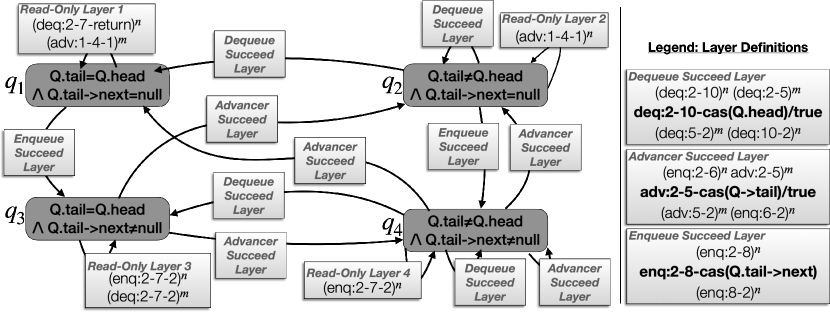
Figure 6: Layer automaton for the Michael/Scott Queue.

6.0.2 2. SLS Synchronous Reservation Queue.

The Scherer-Lea-Scott (SLS) queue [43] builds on MSQ, and it adds support for synchronous operations. If the queue is empty, then dequeuers make reservations and then spin waiting for an enqueuer to fulfill the reservation. Dually, enqueuers put elements into the queue and then spin waiting for a dequeuer to consume the element, after which point the enqueuer advances the head pointer.

The SLS queue demonstrates that a method implementation could consist of sequentially composed paths which define different layers. As we will see, advancing the tail pointer (and the head pointer) are subpaths of method implementation. Moreover, the synchronous behavior involves busy-wait/blocking during the implementation, after which point further paths are executed.

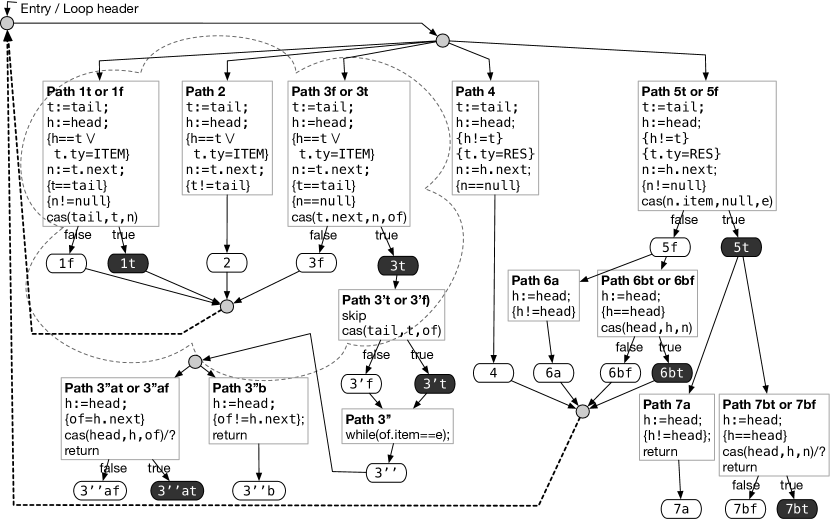
Figure 7: The implementation of a synchronous queue due to Scherer et.al [43].

The implementation of the SLS queue is illustrated in Fig. 7 (the source code is given in Apx. 0.F). This diagram is like a control-flow graph (entry point, loop header, branch/merge points, etc.), but with some flattening to make paths more explicit. Paths are identified where they end, with write paths denoted as and local paths as . Two paths that share a prefix and differ only based on a CAS result are denoted with a single box, but with true/false exit arcs, e.g.,   and . Note that, unlike Treiber’s stack or the MSQ, in the SLS queue a method invocation could involve a series of paths, e.g.,  the sequence $\leavevmode\hbox to14.28pt{\vbox to8.84pt{\text{[drawing]}}}\mathchar 24635\relax\;\leavevmode\hbox to17.37pt{\vbox to9.34pt{\text{[drawing]}}}\mathchar 24635\relax\;\leavevmode\hbox to16.26pt{\vbox to9.34pt{\text{[drawing]}}}\mathchar 24635\relax\;\leavevmode\hbox to25.15pt{\vbox to9.34pt{\text{[drawing]}}}$ involves three write operations.

For lack of space, the explanation of the SLS queue implementation in terms of this diagram is given in Apx. 0.F.1. Briefly, the cloud-surrounded area in the upper left-hand half of the diagram is essentially MSQ and it involves manipulating a list of nodes that are items with a dummy head node. There is a synchronous blocking on path . Alternatively the queue may be a list of reservations, and the right-hand paths attempt to fulfill a dequeuer’s reservation by swapping null for an element. The implementation of dequeue is a sort of dual, omitted for lack of space. Below we denote paths such as to mean the dequeue dual of enqueue’s ; layers typically involve both enqueue and dequeue paths.

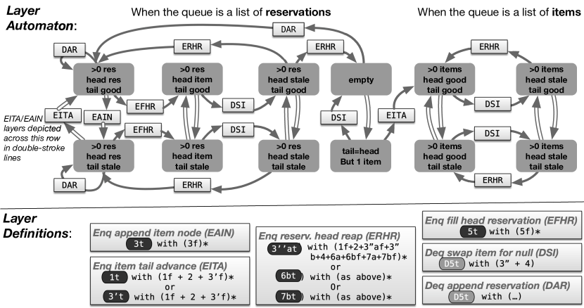
Figure 8: Layer automaton for the synchronous SLS queue. Layers’ acronyms and their definitions are given in the lower half of the figure. For conciseness, layer definitions do not split the prefix/suffix of the read paths. Note that the EITA and EAIN layer transitions occur repeatedly between lower and upper nodes, as indicated.

Quotient. The layer expression for the SLS queue is depicted as a layer automaton in Fig. 8. The automaton states differentiate between whether the queue is empty (the “empty” state), or a single item has been added (“tail=head but 1 item”) or whether the queue consists of reservations (left hand region) or of items (right hand region). In each of those regions, it is relevant as to whether the head pointer is stale or not, as well as whether the tail pointer is stale or not. When the queue is a list of reservations, the head node could point to a node with a reservation (first column of states) or a recently fulfilled reservation node with an item (second column of states) or a null node when the item has been consumed by a dequeuer (third column of states). Technically the states require one further predicate to indicate whether there is currently a thread at location , omitted for lack of space. This is needed because the subsequent paths use the local variable t which is an old read done in the previous path. This is acceptable because it is only possible that one thread can be at location so the old read is still valid during the subsequent path. Typically we have found that implementations do not perform such “old reads” which are only correct as a result of very delicate reasoning. The layers are defined at the bottom of Fig. 8. The are marked with the relevant black-circle write paths. The notation indicates the write path, along with a starred-union of corresponding local paths. For enqueue, the write path forms the EAIN layer in which a single item node is appended, causing concurrent paths to fail. We illustrate the two dequeue layers that correspond to consuming an item (DSI) and appending a reservation (DAR). Dequeue also consists of head/tail advancement layers not depicted here because they are the same as the enqueue advancement layers.

Comparison with the authors’ proof. We found that the layer quotient corresponds well to the informal correctness proof presented by Scherer et al. [43]. In Apx. 0.G we list the authors’ prose and correlate that prose with the quotient. Briefly, the authors’ prose communicates, inter alia, where linearization points occur, which aspects of the data/state are important, and how a change in one thread impacts others. For example, SLS write, “The reservation linearization point for this code path occurs at [the CAS of ] when we successfully insert our offering into the queue.” This sentence seems to identify an important moment, i.e.,  layer EAIN, when we insert the node into the queue. It also indicates what data is important: the tail’s next pointer becoming non-null. Finally, it says that the write of is a linearization point and, since path is atomic, we can treat the entire path as a linearization point. As another example, the SLS sentence “A successful followup linearization point occurs when we notice at line 13 that our data has been taken” indicates how the local path is part of a layer in which the dequeuer’s CAS replaces an element with null.

6.0.3 3. The Herlihy-Wing Queue.

The quotients of some data structures cannot be represented using layer automata. The Herlihy-Wing Queue [17] is one such example and it is notorious for linearization points that depend on the future and that can not be associated to fixed statements, see e.g. [42]! The queue is implemented as an array of slots for items, with a shared variable back that indicates the last possibly non-empty slot. An enq atomically reads and increments back and then later stores a value at that location. A deq repeatedly scans the array looking for the first non-empty slot in a doubly-nested loop. We show that the Herlihy-Wing queue quotient can be abstracted by an expression $\left(\texttt{deqF}^{*}\cdot(\texttt{enqI})^{+}\cdot\texttt{enqW}^{*}\cdot\texttt{deqT}^{*}\right)^{*}$, where deqF captures dequeue scans that need to restart, deqT scans succeed, enqI reads/increments back and enqW writes to the slot. For lack of space, a detailed discussion about how this expression abstracts the quotient is given in Apx. 0.G.1. Importantly, linearization points in executions represented by this expression are fixed, drastically simplifying reasoning from the general case where they are non-fixed.

7 Experiments

Implementation. We built a proof-of-concept implementation of our algorithm, called Cion in just over 1,000 lines of new OCaml code, using CIL and Ultimate [13]. Cion will soon be released publicly on GitHub, with an artifact of the experiments also available. (For reviewing, benchmark sources and Cion’s LaTeX output are available in the supplemental materials.)

	States	# Paths		# Trans.	# Layers	Time	# Solver
Example	$\mid\!\mathcal{Q}\!\mid$	# $k_{l}$	# $k_{w}$	$\mid\!\delta\!\mid$	$\mid\!\Lambda(O)\!\mid$	(s)	Queries
bench/evenodd.c	2	2	2	6	3	50.8	32
bench/counter.c	2	3	2	6	4	63.3	36
bench/descriptor.c	4	6	2	6	5	155.2	74
bench/treiber.c	2	3	2	6	4	70.3	37
bench/msq.c	4	9	3	17	7	437.6	314
bench/listset.c	7	6	2	77	8	466.9	532

Figure 9: Evaluation of Cion applied to the case studies and examples in this paper.

Experiments. We applied Cion to the Counter from Section 2, the three case studies in Section 6 (Treiber’s Stack, Michael/Scott Queue, List Set) as well as a counter that distinguishes Even-vs-Odd, and a mutual exclusion example (descriptor) where locks are acquired with ARWs. The benchmarks are available in the supplemental materials. The results are summarized in Fig. 9 and the output of Cion is displayed in tooloutput.pdf in the supplemental materials. For each benchmark, we report the number of automaton States $\mid\!\mathcal{Q}\!\mid$, the number of local Paths $\#k_{l}$ and number of write paths $\#k_{w}$. We then report the number of Transitions $\mid\!\delta\!\mid$ in the automata constructed by Cion and the number of Layers, as well as the wall-clock Time in seconds, and the number of Queries made to the solver (Ultimate). For MSQ, Ultimate needed to use MathSAT for one feasibility check (the 62nd solver query). Since there is no distribution of MathSAT 5 compiled to ARM architecture, we ran Ultimate on an X86 Linux machine for that single check but the solving time for that one query was negligible. The results show that Cion is able to efficiently generate layer automata for several important and challenging concurrent objects.

8 Related work

Linearizability proofs. Program logics for compositional reasoning about concurrent programs and data structures have been studied extensively. Improving on the classical Owicki-Gries [37] and Rely-Guarantee [18] logics, various extensions of Concurrent Separation Logic [3, 4, 35, 38] have been proposed in order to reason compositionally about different instances of fine-grained concurrency, e.g. [19, 20, 27, 41, 44, 34, 40, 46, 6, 48, 47, 26]. We think of our work as addressing a different class of users compared to such work. Proof systems such as those mentioned above are great in mechanizing/automating a proof and the current users are mostly verification experts. Our work defines a form of reduction to a representative set of interleavings, which are closer to intuitive arguments used by algorithm designers.

Reduction. Lipton’s reduction theory [28] introduced the concept of movers, atomic operations that may execute earlier or later than other concurrently-executing operations without changing the final state, to define a program transformation that creates atomic blocks of code. QED [8] expanded the scope of Lipton’s theory by introducing iterated application of reduction and abstraction over gated atomic actions. CIVL [12] builds upon the foundation of QED, adding invariant reasoning and refinement layers [24, 25]. Reasoning about concurrent programs via simplifying program transformations has also been adopted in the context of mechanized proofs, e.g., [5]. Inductive sequentialization [23] builds upon this prior work, and introduces a new scheme for reasoning inductively over unbounded concurrent executions. The main focus of these works is to define generic proof rules to prove soundness of such program transformations, whose application does however require carefully-crafted artifacts such as abstractions of program code or invariants. Our work takes a different approach and tries to distill common syntactic patterns of concurrent objects into a simpler reduction argument. Our reduction is not a form of program transformation since quotient executions are interleavings of actions in the implementation.

9 Conclusion

We have shown that reasoning about many concurrent algorithms can be simplified by referring to execution quotients and their abstractions in terms of regular or context-free languages. In this way, intuitive reasoning about how few threads interact can more easily generalize the proofs over arbitrary interleavings. We demonstrate that this applies to several canonical examples including Treiber’s Stack, Michael/Scott Queue, the Scherer-Lea-Scott, and a concurrent linked-list Set, but also to the Herlihy-Wing Queue which is often used as a benchmark of difficult to reason about objects.

We hypothesize that quotient reductions could also improve the scalability of other existing concurrency techniques and tools such as those for progress properties, race detection, and even model checking (testing) techniques like context-bounding. In the future we aim to explore how formalisms and tools in those domains can be adapted and applied to quotients rather than enumerating interleavings in the original implementation.

Appendix 0.A Unabridged Concurrent Object Semantics

We define an operational semantics for concurrent objects as sets of executions that interleave steps of a number of method invocations executed by different threads. For simplicity, we assume that every thread invokes a single method, which is without loss of generality provided that thread ids are modeled as additional inputs. Method implementations are assumed to be given as KAT expressions, as described in Section 3.

Client environments.   An object $O$ is acted on by a finite environment $\mathcal{E}:\mathcal{T}\rightarrow O\times\overline{\mathit{Val}}$, specifying which threads invoke which methods, with which argument values. We use $\mathcal{T}$ to denote the set of thread ids, and $\mathit{Val}$ an unspecified set of values ($\overline{\mathit{Val}}$ denotes the set of tuples of values). We assume that $\mathcal{T}$ is equipped with a total order $<$ that will be used to define representatives of equivalence classes up to symmetry (renaming of thread ids).

States.   We assume that each test or action in a method implementation acts on a local state, whose content can be accessed only by the thread executing that test/action, and possibly a shared state which can be read or modified by any thread in the environment. As expected, we assume that each local state contains a valuation for the arguments of an invocation $\vec{x}$ and, once a thread has finished its execution, its local state contains the return values $\vec{v}$. A precise formalization of local/shared states is irrelevant to our development and we omit it for readability. Let $\Sigma_{lo}$ and $\Sigma_{gl}$ denote the set of local and shared states, respectively.

A thread executes an implementation given by a KAT expression $k$, according to the rules below. We assume that semantics of tests $\llbracket b\rrbracket:(\Sigma_{lo}\times\Sigma_{gl})\rightarrow\mathbb{B}$ and actions $\llbracket a\rrbracket:(\Sigma_{lo}\times\Sigma_{gl})\rightarrow(\Sigma_{lo}\times\Sigma_{gl})$ is provided (or generated from the language/program).

Non-deterministic single-thread execution.   Given an environment $\mathcal{E}$, a step of a single thread $t$ is a relation on $\Sigma_{lo}\times\Sigma_{gl}\times(\mathcal{K}\cup\{\bot\})$ where $\bot$ indicates that a thread has completed. We denote this relation as $\sigma_{l},\sigma_{g},k\downarrow_{\ell}\sigma_{l}^{\prime},\sigma_{g}^{\prime},k^{\prime}$, which optionally involve label $\ell$. Labels are taken from the set of possible labels $\mathcal{L}\subseteq\textsf{A}\cup\textsf{B}\cup\textsf{inv}\;m(\vec{v})\cup\textsf{ret}(\vec{v})\cup\langle\!\!\langle b\cdot a\rangle\!\!\rangle$ which includes primitive actions, primitive tests, invocations, returns or ARWs. (We here write $\textsf{inv}\;m(\vec{v})$ with free variables to refer to the set of all invocations and similar for returns and ARWs.) The labeled single-step semantics are now defined inductively on $k$ as follows:

$$\sigma_{l}^{0},\sigma_{g},\epsilon\downarrow_{\textsf{inv}\;m(\vec{v})}\sigma_{l}^{0}[\mathit{args}_{i}\mapsto v_{i}],\sigma_{g},k_{m}\mathcal{E}(t)=(m(\vec{x})/\vec{v}:k_{m},\vec{v})\qquad\sigma_{l},\sigma_{g},\textsf{ret}(\vec{v})\downarrow_{\textsf{ret}(\vec{v})}\sigma_{l},\sigma_{g},\bot\vec{v}=\sigma_{l}(\vec{v})$$

$$\sigma_{l},\sigma_{g},k+k^{\prime}\downarrow\sigma_{l},\sigma_{g},k\qquad\sigma_{l},\sigma_{g},k+k^{\prime}\downarrow\sigma_{l},\sigma_{g},k^{\prime}\qquad\sigma_{l},\sigma_{g},k\cdot k^{\prime}\downarrow\sigma_{l}^{\prime},\sigma_{g}^{\prime},k^{\prime}\sigma_{l},\sigma_{g},k\downarrow\sigma_{l}^{\prime},\sigma_{g}^{\prime},1$$

$$\sigma_{l},\sigma_{g},k^{*}\downarrow\sigma_{l},\sigma_{g},k\cdot k^{*}\qquad\sigma_{l},\sigma_{g},k^{*}\downarrow\sigma_{l},\sigma_{g},1$$

$$\sigma_{l},\sigma_{g},a\downarrow_{a}\sigma_{l}^{\prime},\sigma_{g}^{\prime},1\lx@proof@logical@and a\neq\langle\!\!\langle(\sigma_{l}^{\prime},\sigma_{g}^{\prime})=\llbracket a\rrbracket(\sigma_{l},\sigma_{g})\qquad\sigma_{l},\sigma_{g},b\downarrow_{b}\sigma_{l},\sigma_{g},1\llbracket b\rrbracket(\sigma_{l},\sigma_{g})=\textsf{true}$$

$$\sigma_{l},\sigma_{g},\langle\!\!\langle b\cdot a\rangle\!\!\rangle\downarrow_{\langle\!\!\langle b\cdot a\rangle\!\!\rangle}\sigma_{l}^{\prime},\sigma_{g}^{\prime},1\lx@proof@logical@and\llbracket b\rrbracket(\sigma_{l},\sigma_{g})(\sigma_{l}^{\prime},\sigma_{g}^{\prime})=\llbracket a\rrbracket(\sigma_{l},\sigma_{g})$$

The first rule is for invocation, assuming that the environment for this thread specifies that $m$ should be invoked with arguments $\vec{v}$. These arguments are recorded in the local state, and an invocation label is generated; $\sigma_{l}^{0}$ is a fixed initial local state. The second rule applies when execution reaches a return statement and a label is generated with the values provided in the local state variables $\vec{v}$. Note that invocation/return labels are not invocation/return actions because they contain values rather than arguments. The subsequent 5 rules are built atop the standard non-deterministic semantics of KAT expressions, without any labels being generated. The last 3 rules are for atomic actions $a$, atomic tests $b$, and ARWs $\langle\!\!\langle b\cdot a\rangle\!\!\rangle$, with the respective labels generated. When a test $b$ does not hold, the successor is undefined (and similar when atomic test $b$ in $\langle\!\!\langle b\cdot a\rangle\!\!\rangle$ does not hold). We further define $\sigma_{l},\sigma_{g},k\Downarrow_{\ell}\sigma_{l}^{n},\sigma_{g}^{n},k^{n}$, relating triples from a sequence $(\sigma_{l},\sigma_{g},k)\downarrow(\sigma_{l}^{1},\sigma_{g}^{1},k^{1})\downarrow\cdots\downarrow_{\ell}(\sigma_{l}^{n},\sigma_{g}^{n},k^{n})$ where only the final $\downarrow$ transition produces a label. (i.e.,  the intermediate label-free nondeterminism has been resolved.)

The rules above give a semantics to steps of a thread assuming a certain shared state $\sigma_{g}$, and can be extended to sequences of steps assuming that the shared state can be changed arbitrarily in between every two steps. Formally, given a KAT expression $k$, an execution of $k$ starting from a local state $\sigma_{l}$ and global state $\sigma_{g}$ is defined as a sequence of triples $\sigma_{l}^{i},\sigma_{g}^{i},k^{i}$ with $0\leq i\leq n$ such that: (1) $\sigma_{l}^{0}=\sigma_{l}$, $\sigma_{g}^{0}=\sigma_{g}$, $k^{0}=k$, (2) $\sigma_{l}^{i},\sigma_{g}^{i},k^{i}\Downarrow_{\ell}\sigma_{l}^{i+1},\sigma_{g}^{i+1},k^{i+1}$ for all $i$ even, (3) $\sigma_{l}^{i}=\sigma_{l}^{i+1}$ and $k^{i}=k^{i+1}$ for all $i$ odd, and (4) $k^{n}=1$. Note that $\sigma_{g}$ is unconstrained in (3).

Example 8

Consider $k_{inc}$ as defined in Example 1 and $\sigma_{l}^{0}=[\texttt{c}\mapsto\textsf{undef}]$ and $\sigma_{g}^{0}=[\texttt{ctr}\mapsto 0]$. Here is one execution of $k_{inc}$:

$$\begin{array}[]{rll}\textrm{Step 0}:&(\sigma_{l}^{0},\sigma_{g}^{0},(\texttt{c:=ctr}\cdots)^{*}),\\ \textrm{Step 1}:&(\sigma_{l}^{0},\sigma_{g}^{0},(\texttt{c:=ctr}\cdots)\cdot(\texttt{c:=ctr}\cdots)^{*}),&\textrm{Unfold * via }\downarrow\\ \textrm{Step 2}:&(\sigma_{l}^{0},\sigma_{g}^{\prime},(\texttt{c:=ctr}\cdots)\cdot(\texttt{c:=ctr}\cdots)^{*}),&\textrm{Global state changed arbitrarily}\\ \textrm{Step 3}:&(\sigma_{l}^{0}[\texttt{c}\mapsto\sigma_{g}^{\prime}(\texttt{ctr})],\sigma_{g}^{\prime},1\cdot(\texttt{c:=ctr}\cdots)^{*}),\ldots&\textrm{Reduce an action via }\downarrow_{\texttt{c:=ctr}}\\ \end{array}$$

0.A.1 Executions, Traces, Linearizability

The set of executions of a concurrent object $O$ in the context of an environment $\mathcal{E}$ are defined as interleavings of single-thread executions, acting on the shared state and their local states, with nondeterministic scheduling.

A configuration $C\in(\sigma_{g},T)$ where $T:\mathcal{T}\rightharpoonup(\Sigma_{lo}\times(\mathcal{K}\cup\{\bot\}))$ comprises a shared state $\sigma_{g}\in\Sigma_{gl}$ and a mapping for each active thread to its local state and current code. The initial configuration is defined by $C_{0}=(\sigma_{g}^{0},\emptyset)$ where $\sigma_{g}^{0}$ is a fixed initial shared state. Let $\mathcal{C}$ denote the set of configurations.

An execution of $O$ is a sequence of configurations and labeled transitions over the threads specified by an environment $\mathcal{E}$. The transition relation $\Rightarrow:\mathcal{C}\times(\mathcal{T}\times\mathcal{L})\times\mathcal{C}$ is defined as:

$$(\sigma_{g},T)\mathrel{\leavevmode\hbox to47.52pt{\vbox to16.15pt{\text{[drawing]}}}}(\sigma_{g}^{\prime},T[t\mapsto(\sigma_{l}^{0}[\mathit{args}_{i}\mapsto v_{i}],k_{m})])\mathcal{E}(t)=(m(\vec{x})/\vec{v}:k_{m},\vec{v})\quad T(t)\mbox{ undefined} \scriptstyle(t:\textsf{inv}\;m(\vec{v}))$$

$$(\sigma_{g},T)\mathrel{\leavevmode\hbox to22.98pt{\vbox to14.26pt{\text{[drawing]}}}}(\sigma_{g}^{\prime},T[t\mapsto(\sigma_{l}^{\prime},k^{\prime})])\lx@proof@logical@and T(t)=(\sigma_{l},k)\sigma_{l},\sigma_{g},k\Downarrow_{\ell}\sigma_{l}^{\prime},\sigma_{g}^{\prime},k^{\prime} \scriptstyle(t:\ell) \scriptstyle(t:\ell)$$

A transition $\mathrel{\leavevmode\hbox to7.37pt{\vbox to7.26pt{\text{[drawing]}}}}$ is possible for any thread whose $k$ is not $\bot$. The first rule models a new thread invoking a method according to the environment. In the second, the thread $t$ takes a $\Downarrow_{\ell}$ step, producing label $\ell$, and the configuration is updated with the new global state and the new $(\sigma_{l}^{\prime},k^{\prime})$ for thread $t$.

Appendix 0.B Proof of Theorem 5.1

We reason by induction on the number of paths in $\Pi(\mathsf{expr})$ in a completed execution $\rho$ of $O$ that are either (1) write paths but they are interleaved with actions of other threads, or (2) local paths but they are interleaved with more than two write paths in $\Pi(\mathsf{expr})$, or with a single write path in $\Pi(\mathsf{expr})$ but together with this path, it does not form a support of a layer in $\mathsf{expr}$.

The base case of the induction is trivial: since every label of a transition in $\rho$ belongs to some path in $\Pi(\mathsf{expr})$, and all paths are interleaved as prescribed by the layers, then clearly, the trace of $\rho$ is in the interpretation of $\mathsf{expr}$.

For the induction step, consider first a write path that is interleaved with actions of other threads. Let $\rho^{\prime}$ be the minimal subsequence of $\rho$ that contains only steps of that path and all the other write paths that interleave with it. By the induction hypothesis, the latter write paths execute without interruption. This execution is feasible starting from the first configuration of $\rho^{\prime}$, because we removed only local actions that do not affect enabled-ness of other concurrently executing steps. Applying the WPC condition, there exists an execution $\rho^{\prime\prime}$ strongly equivalent to $\rho^{\prime}$ where all paths execute without interruption. Since $\rho^{\prime\prime}$ passes through the same sequence of shared states (modulo stuttering) it can “replace” $\rho^{\prime}$ in $\rho$. The trace of the obtained execution is a sequence of layers which ends the proof.

Second, consider a local path that is interleaved with more than two write paths. Similarly to the previous case, one can extract only the steps of that path and all the other write paths with which it interleaves, apply the LPC condition to produce an equivalent sub-execution where that path interleaves with at most one other write path, and then, re-insert the obtained sub-execution into the original execution.

Appendix 0.C Michael-Scott Queue layer automaton details

The write operations in the layers induce the state changes as shown by the various edges in Fig. 6. For example, the Dequeue Succeed Layer can move from automaton state $q_{2}$ to automaton state $q_{1}$. Naturally, some edges are not enabled. For example, there is no edge from $q_{1}$ to $q_{2}$, because the latter is not reachable from the former via a single write path/layer. Also, while there are outbound edges from $q_{1}$, there is no layer involving a deq write operation (since the queue is empty). Other layers self-loop, such as the Dequeue Succeed Layer self-loop at $q_{4}$.

There are also four local layers that self-loop. These involve local paths that return (e.g.,  Read Only Layer 1 where deq returns because the queue is empty) or paths that loop while waiting (e.g.,  Read Only Layer 3 where enq awaits the advancer thread).

The layer quotient as represented in this layer-automaton is in some sense not optimal because some pairs of write paths commute, e.g.,  enq writing to Q.tail and deq writing to Q.head when the queue is non-empty. However, in these circumstances the overall enq/deq commute in the sequential semantics of the object. Commuting these write linearization points in the layers corresponds to commuting the overall methods. Consequently, the layer quotient can be seen as optimal modulo method-level commutativity.

Lemma 1

The above layer automaton is an abstraction of a quotient for Michael-Scott Queue.

Proof by the methodology of Def. 5.1. (WPC) For the deq successful CAS on Q.head and adv successful CAS on Q.tail, old reads are not possible because every CAS changes those pointers to fresh values. Thus, if the CAS was successful, the read must be in the current layer (there are no other successful CASs in between). The enq CAS on Q.tail->next is similar to Treiber’s stack: Q.tail->next is only written once, so any old value of Q.tail->next will have the same value in the current layer so an old read can move to the current layer. Furthermore, if there was an old read of Q.tail, the value of Q.tail could not have changed without Q.tail->next first having been changed.

(LPC) CAS operations always change the value so it is always possible to move a late “failing” CAS to the left so that it occurs after the first successful CAS following the previous reads in the same iteration.

Note that the Advancer Succeed Layer in reality cannot self-loop from $q_{3}$ because an invariant of the MSQ is that Q.tail can only lag behind by one link in the list. This happens because weakest preconditions from a $\mathit{true}$ postcondition are over-approximate and did not include complicated invariant reasoning to accurately express the single-link lag condition. Consequently this layer automaton (soundly) over-approximates the executions of the MSQ.

Appendix 0.D Layers for Treiber’s Stack

Recall the implementation of Treiber’s stack [45], stored as a linked list from a global pointer top, and manipulated as follows:
⬇ 1void push(int item){ while(1){ 2 node_t* n = malloc(...); 3 n->val = item; 4 node_t* oldTop = top; 5 n->next = oldTop; 6 if(CAS(top,oldTop,n) ret; 7} } ⬇ 1int pop(){ while(1){ 2 node_t* oldTop = top; 3 if(oldTop==NULL) { ret 0; } 4 newTop = oldTop->next; 5 if(CAS(top,oldTop,newTop) ret oldTop->val; 6} }

The states for the layer-automaton of the Treiber’s Stack (derived from the pre-conditions of successful push and pop operations) are simply top=null and top$\neq$null. The Treiber stack can thus be decomposed into a layer automaton as follows:

Above the automaton states are given in rounded dark boxes, and edges are labeled with layers. We abbreviate local paths using source code line numbers rather than KAT expressions. For example pop:2-5 means the path starting at the beginning of Line 2 of pop and proceeding to the beginning of Line 5. Layer 1 is a local layer, in which the state is top=null. In this layer, there is only one local path from pop that is enabled for some $n$ threads and it pertains to returning 0 to indicate empty. Layer 2 occurs from a state where top$\neq$null and the pop ARW action for the compare-and-swap occurs, causing $n$ other pushes’ and $m$ pops’ CAS attempts to fail (on their lines 6 and 5, respectively) and thus they restart (transition back to their respective Line 2s). The write path is in bold. The other layers are similar, with a single pop or push ARW invalidating other pop/push attempts. Layer 2 occurs as a label in two different transitions. Layer 5 self-loops at state top$\neq$null, which abstracts over all non-empty stacks.

Lemma 2

The above layer automaton is an abstraction of a quotient for Treiber’s stack.

Proof follows the methodology of Def. 5.1. Per WPC, we must show that an old read of top and top->next, with then arbitrarily many write paths interleaved, can be moved to the right just before the successful CAS (an unsuccessful CAS belongs to a local path, discussed next). The successful CAS checks that top is unchanged since the old read. Moreover, since top->next is only written once, if top is unchanged then top->next must also be unchanged. Therefore both old reads could be moved to the right just before the successful CAS, and a whole write path can be assumed to execute without interruption.

Per LPC, requiring that each local path, pops returning 0 or iterations with failed CASs, can be re-ordered to interleave with at most one write path. Iterations where a pop returns 0 perform a single access to shared-memory (reading top) and therefore, they can be assumed to execute without interruption. The failed CAS in an iteration can be re-ordered to occur just after the first successful CAS that follows the read of top in the same iteration. This holds because in Treiber’s stack successful CAS operations always mutate top to a fresh value (assuming memory freshness).

Appendix 0.E Layers of the List Set

Below we return to the List Set example of Sec. LABEL:sec:listset and describe the layer expressions and proof that they abstract the List Set quotient. This example is a Set object implemented as a sorted linked list [36], which involves a read-only traversal locate, and then small atomic sections to link/unlink nodes (for insert/delete, respectively). locate traverses the list from the head and returns a pair of nodes (x,y) such that y has the key of interest or else x points to the last node whose key is below k. It is implemented as a loop that may perform an unbounded number of shared-memory reads. We assume that it is abstracted with the postcondition at line 3 in insert stating that y is the successor of x, the input k is in between x.key and y.key, and that at some point between the invocation of the operation and “now”, x resides on a valid search path for k that starts at the head of the list, denoted as $\topinset{$\cdot$}{$\Diamond$}{3pt}{}\texttt{head}\stackrel{{\scriptstyle\texttt{k}}}{{\rightarrow}}\texttt{x}$. Recent work [9, 10] shows that this postcondition can be derived easily by showing that roughly, list nodes are never updated once they become unreachable. Therefore, the implementations of insert and delete are as follows:

⬇ 1int insert(int k) { while(1) { 2 struct node_t *z = ...; 3 assume $\texttt{x.next = y}\land\texttt{x.key}<\texttt{k}\leq\texttt{y.key}\land\topinset{$\cdot$}{$\Diamond$}{3pt}{}\texttt{head}\stackrel{{\scriptstyle\texttt{k}}}{{\rightarrow}}\texttt{x}$ 4 atomic { 5 if (x->next == y && x->del == 0) { 6 if (y->key != k) { 7 z->next = y; 8 x->next = z; 9 return 1; 10 } else { return 0; } 11 } 12} }

⬇ 1int delete(int k) { while(1) { 2 assume $\texttt{x.next = y}\land\texttt{x.key}<\texttt{k}\leq\texttt{y.key}\land\topinset{$\cdot$}{$\Diamond$}{3pt}{}\texttt{head}\stackrel{{\scriptstyle\texttt{k}}}{{\rightarrow}}\texttt{x}$ 3 atomic { 4 if(x->next == y && x->del == 0) { 5 if (y->key == k) { 6 y->del = 1; 7 x->next = y->next; 8 return 1; 9 } else { return 0; } 10 } 11 } 12} }

The insert method will link a node z in between x and y, provided that k wasn’t already in the list. The delete method returns 0 if the element wasn’t in the list and otherwise, marks node y for deletion, and then updates x to skip past node y. The delete method marks deleted nodes with a del flag before they are unlinked. Because delete marks deleted nodes’ del fields, a concurrent locate that has just found this node, but was then preempted by delete, will return a node that’s marked as deleted and unlinked, not simply unlinked.

As we discuss below, for List Set the layer expressions based on interleavings of two threads generalizes to arbitrary threads. We thus define the states of the automaton in terms of the possible values from the perspective of one reader and one writer. In these states below, x_w denotes the writer’s x, x_r denotes the reader’s x and similar for the other variables. The x and y variables are existentially-quantified in the pre-conditions because they are method-local variables and not inputs. We omit the sub-formula $\topinset{$\cdot$}{$\Diamond$}{3pt}{}\texttt{head}\stackrel{{\scriptstyle\texttt{k}}}{{\rightarrow}}\texttt{x}$ because this condition does not affect the enabled status of a layer.

$$\footnotesize\begin{array}[]{rll}\mathit{q}^{1}&=&\llbracket\textrm{$\exists${x${}_{r}$},{y${}_{r}$}.\ {x${}_{r}$->next=y${}_{r}$ $\wedge$ !x${}_{r}$->del $\wedge$ k${}_{r}$=y${}_{r}$->key}}\rrbracket,\\ \mathit{q}^{2}&=&\llbracket\textrm{$\exists${x${}_{r}$},{y${}_{r}$}.\ {x${}_{r}$->next=y${}_{r}$ $\wedge$ !x${}_{r}$->del $\wedge$ x${}_{r}$->key~{}<~{}k${}_{r}$~{}<~{}y${}_{r}$->key}}\rrbracket,\\ \mathit{q}^{3}&=&\llbracket\textrm{$\exists${x${}_{r}$},{y${}_{r}$},{x${}_{w}$},{y${}_{w}$}.\ {x${}_{w}$->next=y${}_{w}$ $\wedge$ !x${}_{w}$->del $\wedge$ x${}_{w}$->key~{}<~{}k${}_{w}$~{}<~{}y${}_{w}$->key $\wedge$}}\\ &&\textrm{{x${}_{r}$=x{\color[rgb]{0,0,1}${}_{w}$} $\wedge$ x${}_{r}$->key~{}<~{}k${}_{r}$~{}<~{}y${}_{r}$->key}}\rrbracket,\\ \mathit{q}^{4}&=&\llbracket\textrm{$\exists${x${}_{r}$},{y${}_{r}$},{x${}_{w}$},{y${}_{w}$}.\ {x${}_{w}$->next=y${}_{w}$ $\wedge$ !x${}_{w}$->del $\wedge$ x${}_{w}$->key~{}<~{}k${}_{w}$~{}<~{}y${}_{w}$->key $\wedge$ }}\\ &&\textrm{{x${}_{r}$=x{\color[rgb]{0,0,1}${}_{w}$} $\wedge$ k${}_{r}$=y${}_{r}$->key}}\rrbracket,\\ \mathit{q}^{5}&=&\llbracket\textrm{$\exists${x${}_{r}$},{y${}_{r}$},{x${}_{w}$},{y${}_{w}$}.\ {x${}_{w}$->next=y${}_{w}$ $\wedge$ !x${}_{w}$->del $\wedge$ k${}_{w}$=y${}_{w}$->key $\wedge$ x${}_{r}$=x{\color[rgb]{0,0,1}${}_{w}$} $\wedge$ }}\\ &&\textrm{{ x${}_{r}$->key~{}<~{}k${}_{r}$~{}<~{}y${}_{r}$->key}}\rrbracket,\\ \mathit{q}^{6}&=&\llbracket\textrm{$\exists${x${}_{r}$},{y${}_{r}$},{x${}_{w}$},{y${}_{w}$}.\ {x${}_{w}$->next=y${}_{w}$ $\wedge$ !x${}_{w}$->del $\wedge$ k${}_{w}$=y${}_{w}$->key $\wedge$ x${}_{r}$=x{\color[rgb]{0,0,1}${}_{w}$} $\wedge$ k${}_{r}$=key}}\rrbracket,\\ \mathit{q}^{7}&=&\llbracket\textrm{$\exists${x${}_{r}$},{y${}_{r}$}.\ {x${}_{r}$->next=y${}_{r}$ $\wedge$ x${}_{r}$->del $\wedge$ x${}_{r}$->key~{}<~{}k${}_{r}~{}\leq~{}$y${}_{r}$->key}}\rrbracket\\ \end{array}$$

With these 7 states, 2 write paths (one from insert, one from delete) and 6 read paths, there are many transitions to consider, although many of them are labeled with the same layer. In fact, the List Set can be decomposed into 8 layers, enumerated below. For lack of space, we omit the automaton, but the definitions, including all 77 feasible transitions, can be seen in the output of our tool (which we discuss in the next section) shown in Apx. A. Below we refer to example transitions in Apx A, denoted $\delta_{i}$.

1. A layer with a delete write path that updates x.next to point to y.next, causing one insert and one delete path to fail when finding x.next$\neq$y.(e.g.,  $\delta_{2}$)

2. A layer with an insert write path that updates x.next to point to z, causing one insert and one delete paths to fail when finding x.next$\neq$y. (e.g.,  $\delta_{9}$)

3. A local layer consisting of one delete path, when the key is not in the set. (e.g.,  $\delta_{31}$)

4. A local layer consisting of one insert path, when the element is already in the set. (e.g.,  $\delta_{47}$)

5. Four local layers consisting of insert or delete paths when the node x is already marked for deletion. (e.g.,  $\delta_{63}$)

Note that insert and delete have more than one control-flow path that “fails” because of the nested conditional inside the atomic read-write.

As in the Michael/Scott queue, here again the layer-quotient is optimal modulo method-level commutativity. At the method-level, operations such as insertion/deletion of different elements commute and their corresponding linearizations can be commuted (different orders of write layers) in the layer quotient.

Lemma 3

The above layer automaton is an abstraction of a quotient for the List Set.

Proof by the methodology of Def. 5.1. To prove the lemma we first note that the post-condition of locate ensures that x was reachable and that y=x->next. In all read and write paths, the ARW checks that y=x->next still holds. Furthermore, an invariant of the implementation is that if x was reachable at some point in the past (i.e.,  when locate executed) and !x->del holds in the atomic section, then x is still reachable in the atomic section (this holds because elements are marked before being unlinked). Therefore, if locate’s postcondition was true in the past, it remains true when the ARW succeeds and the assume can be reordered to occur just before it. For local paths, as in previous cases, a failed ARW can be commuted to the left to occur just after the first ARW that modifies the location x.

Appendix 0.F SLS queue source code

Below is the implementation of the Scherer et al. [43] queue. Path labels such as or are included to indicate which paths from Sec. LABEL:sec:resqueue correspond to those program locations, where possible. (We have slightly refactored the second portion of the implementation in our path graph.)

⬇

1public void enq(T e) {

2 Node offer = new Node(e, NodeType.ITEM);

3 while (true) {

4 Node t = tail.get(), h = head.get();

5 if (h == t t.type == NodeType.ITEM) {

6 Node n = t.next.get();

7 if (t == tail.get()) {

8 if (n != null) {

9 tail.compareAndSet(t, n); ,

10 } else if (t.next.compareAndSet(n, offer) ) {

11

12 tail.compareAndSet(t, offer); ,

13 while (offer.item.get() == e);

14 h = head.get();

15 if (offer == h.next.get()) {

16 head.compareAndSet(h, offer); return; ,

17 } else { return; }

18 } else { restart }

19 } else { restart }

20 } else {

21 Node n = h.next.get();

22 if (t != tail.get() h != head.get() n == null ) {

23 continue;

24 }

25 boolean success = n.item.compareAndSet(null, e); ,

26 head.compareAndSet(h, n); ,

27 if (success)

28 return; , ,

29 else

30 restart , ,

31 }

32 }

33}

0.F.1 SLS queue implementation graph

Figure 10: (Reproduction of Fig. 7: The implementation of a synchronous queue due to Scherer et.al [43].)

We describe the implementation in Fig. 7, beginning with the cloud-surrounded area in upper left-hand half of the diagram which is, essentially, the Michael-Scott queue. In this region the queue is a list of items (with a dummy head node), whereas the new portions of the implementation apply when the queue is a list of reservations. Paths and attempt to advance the tail pointer. Path is interrupted by a recently changed tail pointer. Paths and attempt to swap tail’s next to their new item offer node. If successful, paths and attempt to advance the tail pointer.

Path is the synchronous part of the algorithm: waiting for an enqueued item to be consumed by a dequeuer. At that point, the head pointer may be stale, and paths , and try to advance the head pointer.

Alternatively the queue may be a list of reservations, again with a dummy head node. Paths and attempt to fulfill a dequeuer’s reservation by swapping null for an element. Path is doomed to restart, while path will soon return. In either case, the enqueue first attempts to advance the head pointer (paths $\leavevmode\hbox to15.39pt{\vbox to8.84pt{\text{[drawing]}}},\leavevmode\hbox to19.32pt{\vbox to9.34pt{\text{[drawing]}}},\leavevmode\hbox to20.15pt{\vbox to9.34pt{\text{[drawing]}}},\leavevmode\hbox to15.39pt{\vbox to8.84pt{\text{[drawing]}}},\leavevmode\hbox to19.32pt{\vbox to9.34pt{\text{[drawing]}}},\leavevmode\hbox to20.15pt{\vbox to9.34pt{\text{[drawing]}}}$).

The implementation of dequeue is a sort of dual operation. When the queue is a non-empty list of items, dequeue tries to take the first item by swapping the head’s next value for null (and then tries to advance the head pointer). When the queue is empty or a list of reservations, dequeue redirects the tail’s next to its new reservation node (and then tries to advance the tail pointer). After appending the reservation, dequeue spins until a value is swapped in, and then tries to advance the head pointer before returning.

Appendix 0.G SLS queue author’s correctness arguments

We review the correctness argument presented by the original authors [43], quoting their prose and discussing how those statements correspond to our quotient proof methodology with layer expressions.

The reservation linearization point for this code path occurs at line 10 when we successfully insert our offering into the queue – Scherer et al. [43]

First, this prose indicates that is a linearization point. The write of is atomic and so this line number has a corresponding location in the layer expression, which is this same linearization point. Second, this prose identifies a layer as an important state change: inserting an offer node into the queue. This is the EAIN layer in our decposition. Third, the prose describes what kind of data change is important: the tail changing to non-null, a distinction we make in the states of our layer automaton.

“A successful followup linearization point occurs when we notice at line 13 that our data has been taken. – Scherer et al. [43]

Similarly here this linearization point appears in a layer where a dequeue mutates the state, and local path is feasible. This prose also identifies important state change: from an item to null.

The other case occurs when the queue consists of reservations (requests for data), and is depicted [below]. – Scherer et al. [43]

In this case, after originally reading the head node (step A), we read its successor (line 21/step B) and verify consistency (line 22). Then, we attempt to supply our data to the head-most reservation (line 25/C). If this succeeds, we dequeue the former dummy node ( 26/D) and return – Scherer et al. [43]

This prose again indicates important state changes, which are reflected as distinct states (and transitions between them) in our layer automata: whether head-most reservation has data supplied and whether the head dummy node needs to be advanced.

If it fails, we need to go to the next reservation, so we dequeue the old dummy node anyway (28) and retry the entire operation (32, 05). – Scherer et al. [43]

This is a description of the failure path $\leavevmode\hbox to13.76pt{\vbox to9.34pt{\text{[drawing]}}}\cdot(\leavevmode\hbox to20.15pt{\vbox to9.34pt{\text{[drawing]}}}+\leavevmode\hbox to19.32pt{\vbox to9.34pt{\text{[drawing]}}}$) and that interference (implicitly) caused by a concurrent cas from .

The reservation linearization point for this code path occurs when we successfully supply data to a waiting consumer at line 25; the followup linearization point occurs immediately thereafter. – Scherer et al. [43]

Again, this prose indicates the important state transition at , replacing a null with an item (as seen in the states of our layer automaton), and corresponding automaton transition for layer EFHR.

0.G.1 The Herlihy-Wing Queue

Recall the queue due to Herlihy and Wing [17], reproduced below:

⬇ 1int deq() { while(1) { 2 assume 0 <= range < back; int j = 0; 3 while(j<range) { 4 v := swap(items[j],null); 5 if (v != null) return v; 6 j++; } 7} }

⬇ 1void enq(int v) { 2 i := back++; 3 items[i] = v; 4}

Enqueue (on the right) reserves the next slot in the array items by atomically reading and incrementing the shared variable back, and then assigns the value to that slot in a second write to the shared state. Meanwhile, dequeue (on the left), in an outer loop reads into range any value strictly smaller than back and then iterates from 0 to range, looking for a slot containing an item to atomically dequeue. For every j, it atomically reads items[j] into v and writes null (written as a swap instruction), and if the read value is not null, it returns it. This is actually a sound abstraction of the original version which assigns back-1 to range instead of any smaller value. Soundness follows easily from the fact that reading a smaller value will only make the dequeue restart more often (perform more traversals in which there is no occupied slot), but not affect safety. In the reasoning below, we will use the fact that such a non-deterministic read commutes to the right of any increment of back (it is a right mover).

We show that the Herlihy-Wing queue quotient can be abstracted by an expression given below. To this end we first, as below in Apx. 0.G.2, prove that any iteration of the dequeue’s outer while(1) loop can be considered atomic, modulo commutative re-orderings. Consequently, there exists a quotient of Herlihy and Wing Queue where outer loop iterations in dequeue are atomic sections. Since items[i] = v steps in enqueues commute (they write on different slots of the array), there exists a quotient where additionally, every sequence of items[i] = v steps before a dequeue iteration that is successful (contains a non null swap) is ordered w.r.t. the array slots that they write. The following expression is an abstraction of such a quotient: $\left(\texttt{deqF}^{*}\cdot(\texttt{enqI})^{+}\cdot\texttt{enqW}^{*}\cdot\texttt{deqT}^{*}\right)^{*}$ where enqI and enqW denote the statements i:=back++ and items[i] = v in enqueue, respectively, and deqT and deqF represent entire iterations of the outer loop in dequeue that end in a return and restarting the loop, respectively. The interpretation of $\texttt{enqW}^{*}$ is refined to be a set of sequences of labels items[i] = v (with thread ids) that are ordered w.r.t. the position $i$ that they write to. Above, we also use straightforward feasibility arguments like “enqueues increment back before writing to items,” and “a deqT must be preceded by a write to items in an enqueue.”

The set of traces represented by this expression admits a “simple” linearization point mapping which identifies enqW and deqT steps with linearization points of enqueues and dequeues, respectively. The restriction to traces in this quotient is instrumental for such a simple linearization point mapping. For arbitrary traces, the Herlihy and Wing Queue is known for having linearization points that depend on the future and that can not be associated to fixed statements, see e.g. [42] !

0.G.2 Proof of atomicity of outer loop

We prove that any iteration of the outer while(1) loop can be considered to be an atomic section, modulo re-orderings of commutative actions. That is, there exists a quotient of this object formed of traces where all steps of such an iteration occur consecutively one after another.

We proceed by induction on the number of steps executing the swap at line 4 in dequeue and that find a non-null value in items[j]. In the base case, i.e., the number of such steps is 0, all the swaps at line 4 in all dequeue invocations find null values. Therefore, any possible write to an items slot (in enqueues) can be re-ordered after all swaps. Now all steps in the same outer loop iteration of a dequeue (the non-deterministic read of back and swaps returning null) can be re-ordered to occur consecutively one after another. In particular this relies on the fact that the non-deterministic read of back can return the same value even if executed after more increments of back. For a trace with $n+1$ swaps returning non-null values, we focus on the first such step. Assume that it is a swap on some position k. All the writes to items slots strictly before k can be re-ordered to the right of this first non-null swap. This relies on the fact that all the other previous swaps return a null value and anyway, do not “observe” these writes. Similarly to the base case, all steps in the same outer loop iteration of a dequeue that completes before this first non-null swap (including) can be re-ordered to occur consecutively one after another. We are again using the fact that swaps read null values and there is no more write on the slots that they read. Now, removing the write to items[k] in enqueue and the dequeue iteration that removes this value from the current trace, we get another feasible trace that has $n$ non-null swaps, for which one can apply the induction hypothesis.

References

• [1] Anderson, C.J., Foster, N., Guha, A., Jeannin, J., Kozen, D., Schlesinger, C., Walker, D.: Netkat: semantic foundations for networks. In: Jagannathan, S., Sewell, P. (eds.) The 41st Annual ACM SIGPLAN-SIGACT Symposium on Principles of Programming Languages, POPL ’14, San Diego, CA, USA, January 20-21, 2014. pp. 113–126. ACM (2014). https://doi.org/10.1145/2535838.2535862, https://doi.org/10.1145/2535838.2535862
• [2] Antonopoulos, T., Koskinen, E., Le, T.C.: Specification and inference of trace refinement relations. Proc. ACM Program. Lang. 3(OOPSLA), 178:1–178:30 (2019). https://doi.org/10.1145/3360604, https://doi.org/10.1145/3360604
• [3] Bornat, R., Calcagno, C., O’Hearn, P.W., Parkinson, M.J.: Permission accounting in separation logic. In: Proceedings of the 32nd ACM SIGPLAN-SIGACT Symposium on Principles of Programming Languages, POPL 2005, Long Beach, California, USA, January 12-14, 2005. pp. 259–270 (2005). https://doi.org/10.1145/1040305.1040327, http://doi.acm.org/10.1145/1040305.1040327
• [4] Brookes, S.D.: A semantics for concurrent separation logic. In: CONCUR 2004 - Concurrency Theory, 15th International Conference, London, UK, August 31 - September 3, 2004, Proceedings. pp. 16–34 (2004). https://doi.org/10.1007/978-3-540-28644-8_2, https://doi.org/10.1007/978-3-540-28644-8_2
• [5] Chajed, T., Kaashoek, M.F., Lampson, B.W., Zeldovich, N.: Verifying concurrent software using movers in CSPEC. In: OSDI (2018), https://www.usenix.org/conference/osdi18/presentation/chajed
• [6] Dragoi, C., Gupta, A., Henzinger, T.A.: Automatic linearizability proofs of concurrent objects with cooperating updates. In: CAV ’13. LNCS, vol. 8044, pp. 174–190. Springer (2013)
• [7] D’Antoni, L., Veanes, M.: The power of symbolic automata and transducers. In: International Conference on Computer Aided Verification. pp. 47–67. Springer (2017)
• [8] Elmas, T., Qadeer, S., Tasiran, S.: A calculus of atomic actions. In: POPL (2009). https://doi.org/10.1145/1480881.1480885
• [9] Feldman, Y.M.Y., Enea, C., Morrison, A., Rinetzky, N., Shoham, S.: Order out of Chaos: Proving Linearizability Using Local Views. In: DISC 2018 (2018)
• [10] Feldman, Y.M.Y., Khyzha, A., Enea, C., Morrison, A., Nanevski, A., Rinetzky, N., Shoham, S.: Proving highly-concurrent traversals correct. Proc. ACM Program. Lang. 4(OOPSLA), 128:1–128:29 (2020). https://doi.org/10.1145/3428196, https://doi.org/10.1145/3428196
• [11] Greenberg, M., Beckett, R., Campbell, E.H.: Kleene algebra modulo theories: a framework for concrete kats. In: Jhala, R., Dillig, I. (eds.) PLDI ’22: 43rd ACM SIGPLAN International Conference on Programming Language Design and Implementation, San Diego, CA, USA, June 13 - 17, 2022. pp. 594–608. ACM (2022). https://doi.org/10.1145/3519939.3523722, https://doi.org/10.1145/3519939.3523722
• [12] Hawblitzel, C., Petrank, E., Qadeer, S., Tasiran, S.: Automated and modular refinement reasoning for concurrent programs. In: CAV (2015). https://doi.org/10.1007/978-3-319-21668-3_26
• [13] Heizmann, M., Chen, Y., Dietsch, D., Greitschus, M., Hoenicke, J., Li, Y., Nutz, A., Musa, B., Schilling, C., Schindler, T., Podelski, A.: Ultimate automizer and the search for perfect interpolants - (competition contribution). In: Beyer, D., Huisman, M. (eds.) Tools and Algorithms for the Construction and Analysis of Systems - 24th International Conference, TACAS 2018, Held as Part of the European Joint Conferences on Theory and Practice of Software, ETAPS 2018, Thessaloniki, Greece, April 14-20, 2018, Proceedings, Part II. Lecture Notes in Computer Science, vol. 10806, pp. 447–451. Springer (2018). https://doi.org/10.1007/978-3-319-89963-3_30, https://doi.org/10.1007/978-3-319-89963-3_30
• [14] Henzinger, T.A., Jhala, R., Majumdar, R., Necula, G.C., Sutre, G., Weimer, W.: Temporal-safety proofs for systems code. In: Computer Aided Verification, 14th International Conference, CAV 2002,Copenhagen, Denmark, July 27-31, 2002, Proceedings. pp. 526–538 (2002)
• [15] Herlihy, M., Shavit, N.: The art of multiprocessor programming. Morgan Kaufmann (2008)
• [16] Herlihy, M., Shavit, N.: The Art of Multiprocessor Programming. Morgan Kaufmann Publishers Inc., San Francisco, CA, USA (2008)
• [17] Herlihy, M., Wing, J.M.: Linearizability: A correctness condition for concurrent objects. ACM Trans. Program. Lang. Syst. 12(3), 463–492 (1990). https://doi.org/10.1145/78969.78972, http://doi.acm.org/10.1145/78969.78972
• [18] Jones, C.B.: Specification and design of (parallel) programs. In: IFIP Congress. pp. 321–332 (1983)
• [19] Jung, R., Krebbers, R., Jourdan, J., Bizjak, A., Birkedal, L., Dreyer, D.: Iris from the ground up: A modular foundation for higher-order concurrent separation logic. J. Funct. Program. 28,  e20 (2018). https://doi.org/10.1017/S0956796818000151, https://doi.org/10.1017/S0956796818000151
• [20] Jung, R., Lepigre, R., Parthasarathy, G., Rapoport, M., Timany, A., Dreyer, D., Jacobs, B.: The future is ours: prophecy variables in separation logic. Proc. ACM Program. Lang. 4(POPL), 45:1–45:32 (2020). https://doi.org/10.1145/3371113, https://doi.org/10.1145/3371113
• [21] Kozen, D.: On kleene algebras and closed semirings. In: Rovan, B. (ed.) Mathematical Foundations of Computer Science 1990, MFCS’90, Banská Bystrica, Czechoslovakia, August 27-31, 1990, Proceedings. Lecture Notes in Computer Science, vol. 452, pp. 26–47. Springer (1990). https://doi.org/10.1007/BFb0029594, https://doi.org/10.1007/BFb0029594
• [22] Kozen, D.: Kleene algebra with tests. ACM Trans. Program. Lang. Syst. 19(3), 427–443 (1997). https://doi.org/10.1145/256167.256195, https://doi.org/10.1145/256167.256195
• [23] Kragl, B., Enea, C., Henzinger, T.A., Mutluergil, S.O., Qadeer, S.: Inductive sequentialization of asynchronous programs. In: Donaldson, A.F., Torlak, E. (eds.) Proceedings of the 41st ACM SIGPLAN International Conference on Programming Language Design and Implementation, PLDI 2020, London, UK, June 15-20, 2020. pp. 227–242. ACM (2020). https://doi.org/10.1145/3385412.3385980, https://doi.org/10.1145/3385412.3385980
• [24] Kragl, B., Qadeer, S.: Layered concurrent programs. In: CAV (2018). https://doi.org/10.1007/978-3-319-96145-3_5
• [25] Kragl, B., Qadeer, S., Henzinger, T.A.: Synchronizing the asynchronous. In: CONCUR (2018). https://doi.org/10.4230/LIPIcs.CONCUR.2018.21
• [26] Krishna, S., Shasha, D.E., Wies, T.: Go with the flow: compositional abstractions for concurrent data structures. PACMPL 2(POPL), 37:1–37:31 (2018). https://doi.org/10.1145/3158125, http://doi.acm.org/10.1145/3158125
• [27] Ley-Wild, R., Nanevski, A.: Subjective auxiliary state for coarse-grained concurrency. In: The 40th Annual ACM SIGPLAN-SIGACT Symposium on Principles of Programming Languages, POPL ’13, Rome, Italy - January 23 - 25, 2013. pp. 561–574 (2013). https://doi.org/10.1145/2429069.2429134, http://doi.acm.org/10.1145/2429069.2429134
• [28] Lipton, R.J.: Reduction: A method of proving properties of parallel programs. Commun. ACM 18(12) (1975). https://doi.org/10.1145/361227.361234
• [29] Mazurkiewicz, A.W.: Trace theory. In: Brauer, W., Reisig, W., Rozenberg, G. (eds.) Petri Nets: Central Models and Their Properties, Advances in Petri Nets 1986, Part II, Proceedings of an Advanced Course, Bad Honnef, Germany, 8-19 September 1986. Lecture Notes in Computer Science, vol. 255, pp. 279–324. Springer (1986). https://doi.org/10.1007/3-540-17906-2_30, https://doi.org/10.1007/3-540-17906-2_30
• [30] Michael, M.M.: ABA prevention using single-word instructions. Tech. Rep. RC 23089, IBM Thomas J. Watson Research Center (January 2004)
• [31] Michael, M.M., Scott, M.L.: Simple, fast, and practical non-blocking and blocking concurrent queue algorithms. In: PODC ’96. pp. 267–275. ACM (1996)
• [32] Michael, M., Scott, M.: Simple, fast, and practical non-blocking and blocking concurrent queue algorithms. In: PODC (1996)
• [33] Moir, M., Shavit, N.: Concurrent data structures. In: Mehta, D.P., Sahni, S. (eds.) Handbook of Data Structures and Applications. Chapman and Hall/CRC (2004). https://doi.org/10.1201/9781420035179.ch47, https://doi.org/10.1201/9781420035179.ch47
• [34] Nanevski, A., Banerjee, A., Delbianco, G.A., Fábregas, I.: Specifying concurrent programs in separation logic: morphisms and simulations. Proc. ACM Program. Lang. 3(OOPSLA), 161:1–161:30 (2019). https://doi.org/10.1145/3360587, https://doi.org/10.1145/3360587
• [35] O’Hearn, P.W.: Resources, concurrency and local reasoning. In: CONCUR 2004 - Concurrency Theory, 15th International Conference, London, UK, August 31 - September 3, 2004, Proceedings. pp. 49–67 (2004). https://doi.org/10.1007/978-3-540-28644-8_4, https://doi.org/10.1007/978-3-540-28644-8_4
• [36] O’Hearn, P.W., Rinetzky, N., Vechev, M.T., Yahav, E., Yorsh, G.: Verifying linearizability with hindsight. In: Richa, A.W., Guerraoui, R. (eds.) Proceedings of the 29th Annual ACM Symposium on Principles of Distributed Computing, PODC 2010, Zurich, Switzerland, July 25-28, 2010. pp. 85–94. ACM (2010). https://doi.org/10.1145/1835698.1835722, https://doi.org/10.1145/1835698.1835722
• [37] Owicki, S.S., Gries, D.: Verifying properties of parallel programs: An axiomatic approach. Commun. ACM 19(5), 279–285 (1976). https://doi.org/10.1145/360051.360224, http://doi.acm.org/10.1145/360051.360224
• [38] Parkinson, M.J., Bornat, R., O’Hearn, P.W.: Modular verification of a non-blocking stack. In: Proceedings of the 34th ACM SIGPLAN-SIGACT Symposium on Principles of Programming Languages, POPL 2007, Nice, France, January 17-19, 2007. pp. 297–302 (2007). https://doi.org/10.1145/1190216.1190261, http://doi.acm.org/10.1145/1190216.1190261
• [39] Pous, D.: Symbolic algorithms for language equivalence and kleene algebra with tests. In: Proceedings of the 42nd Annual ACM SIGPLAN-SIGACT Symposium on Principles of Programming Languages. pp. 357–368 (2015)
• [40] Raad, A., Villard, J., Gardner, P.: Colosl: Concurrent local subjective logic. In: Programming Languages and Systems - 24th European Symposium on Programming, ESOP 2015, Held as Part of the European Joint Conferences on Theory and Practice of Software, ETAPS 2015, London, UK, April 11-18, 2015. Proceedings. pp. 710–735 (2015). https://doi.org/10.1007/978-3-662-46669-8_29, https://doi.org/10.1007/978-3-662-46669-8_29
• [41] da Rocha Pinto, P., Dinsdale-Young, T., Gardner, P.: Tada: A logic for time and data abstraction. In: ECOOP 2014 - Object-Oriented Programming - 28th European Conference, Uppsala, Sweden, July 28 - August 1, 2014. Proceedings. pp. 207–231 (2014). https://doi.org/10.1007/978-3-662-44202-9_9, https://doi.org/10.1007/978-3-662-44202-9_9
• [42] Schellhorn, G., Wehrheim, H., Derrick, J.: How to prove algorithms linearisable. In: Computer Aided Verification - 24th International Conference, CAV 2012, Berkeley, CA, USA, July 7-13, 2012 Proceedings. pp. 243–259 (2012)
• [43] Scherer III, W.N., Lea, D., Scott, M.L.: Scalable synchronous queues. In: Proceedings of the eleventh ACM SIGPLAN symposium on Principles and practice of parallel programming. pp. 147–156 (2006)
• [44] Sergey, I., Nanevski, A., Banerjee, A.: Specifying and verifying concurrent algorithms with histories and subjectivity. In: Programming Languages and Systems - 24th European Symposium on Programming, ESOP 2015, Held as Part of the European Joint Conferences on Theory and Practice of Software, ETAPS 2015, London, UK, April 11-18, 2015. Proceedings. pp. 333–358 (2015). https://doi.org/10.1007/978-3-662-46669-8_14, https://doi.org/10.1007/978-3-662-46669-8_14
• [45] Treiber, R.K.: Systems programming: Coping with parallelism. Tech. Rep. RJ 5118, IBM Almaden Research Center (APR 1986)
• [46] Turon, A., Dreyer, D., Birkedal, L.: Unifying refinement and hoare-style reasoning in a logic for higher-order concurrency. In: ACM SIGPLAN International Conference on Functional Programming, ICFP’13, Boston, MA, USA - September 25 - 27, 2013. pp. 377–390 (2013). https://doi.org/10.1145/2500365.2500600, http://doi.acm.org/10.1145/2500365.2500600
• [47] Vafeiadis, V.: Modular fine-grained concurrency verification. Ph.D. thesis, University of Cambridge (2008)
• [48] Vafeiadis, V.: Shape-value abstraction for verifying linearizability. In: VMCAI ’09: Proc. 10th Intl. Conf. on Verification, Model Checking, and Abstract Interpretation. LNCS, vol. 5403, pp. 335–348. Springer (2009)