GAR: A Revisit to the Classic Linear Autoregressive Model And Its Application To Multi-Fidelity Problems

GAR: Generalized Linear Autoregressive Model

GAR: Generalized Autoregression
for Multi-Fidelity Fusion

GAR: Generalized Autoregression for Multi-Fidelity Fusion

GAR: Generalized Autoregression for Multi-Fidelity Fusion

GAR: Generalized Autoregression
for Multi-Fidelity Fusion

Abstract

In many scientific research and engineering applications where repeated simulations of complex systems are conducted, a surrogate is commonly adopted to quickly estimate the whole system. To reduce the expensive cost of generating training examples, it has become a promising approach to combine the results of low-fidelity (fast but inaccurate) and high-fidelity (slow but accurate) simulations. Despite the fast developments of multi-fidelity fusion techniques, most existing methods require particular data structures and do not scale well to high-dimensional output. To resolve these issues, we generalize the classic autoregression (AR), which is wildly used due to its simplicity, robustness, accuracy, and tractability, and propose generalized autoregression (GAR) using tensor formulation and latent features. GAR can deal with arbitrary dimensional outputs and arbitrary multi-fidelity data structure to satisfy the demand of multi-fidelity fusion for complex problems; it admits a fully tractable likelihood and posterior requiring no approximate inference and scales well to high-dimensional problems. Furthermore, we prove the autokrigeability theorem based on GAR in the multi-fidelity case and develop CIGAR, a simplified GAR with the exact predictive mean accuracy with computation reduction by a factor of $d^{3}$, where $d$ is the dimensionality of the output. The empirical assessment includes many canonical PDEs and real scientific examples and demonstrates that the proposed method consistently outperforms the SOTA methods with a large margin (up to 6x improvement in RMSE) with only a couple high-fidelity training samples.

1 Introduction

The design, optimization, and control of many systems in science and engineering can rely heavily on the numerical analysis of differential equations, which is generally computationally intense. In this case, a data-driven surrogate model is used to approximate the system based on the input-output data of the numerical solver and to help improve convergence efficiency where repeated simulations are required, e.g., in Bayesian optimization (BO) [1] and uncertainty analysis (UQ) [2].

With the surrogate model in place, the remaining challenge is that executing high-fidelity numerical simulations to generate training data can still be very expensive. To further reduce the computational burden, it is possible to combine low-fidelity results to make high-fidelity predictions [3]. More specifically, low-fidelity solvers are normally based on simplified PDEs (e.g., reducing the levels of physical detail) or simple solver setup (e.g., using a coarse mesh, a large time step, a lower order of an approximating basis, and a higher error tolerance). They provide fast but inaccurate solutions to the original problems whereas the high-fidelity solvers are accurate yet expensive. The multi-fidelity fusion technique works similar to transfer learning to utilize many low-fidelity observations to improve the accuracy when using only a few high-fidelity samples. In general, it involves constructions of surrogates for different fidelities and a cross-fidelity transition process. Due to its efficiency, multi-fidelity method has attracted increasing attention in BO [4, 5], UQ [6, 7], and surrogate modeling [8, 9]. We refer to [10, 11] for a great review.

Despite the success of many state-of-the-art (SOTA) approaches, they normally assume that (1) the output dimension is the same and aligned across all fidelities, which generally does not hold for multi-fidelity simulation where the output are quantities at nodes that are naturally not aligned; (2) the high-fidelity samples’ corresponding inputs form a subset of the low-fidelity inputs; and (3) the output dimension is small, which is not practical for scientific computing where dimension can be 1-million (for a $100\times 100\times 100$ spatial-temporal field). These assumptions seriously hinder their applications for practical problems, e.g., MRI imaging and solving PDEs in scientific computation.

To resolve these challenges, previous work either uses interpolation to align the dimension [12, 9] or relies on approximate inference with brutal simplification [8, 13], leading to inferior performance. We notice that the classic autoregression (AR), which is widely used due to its simplicity, robustness, accuracy, and tractability, consistently shows robust and top-tier performance for different datasets in the literature, despite its incapability for high-dimensional problems. Thus, instead of proposing another ad-hoc model with pre-processing and simplification (leading to models that are difficult to tune and generalize poorly), we generalize AR with tensor algebra and latent features and propose generalized autoregression (GAR), which can deal with arbitrary high-dimensional problems without the subset multi-fidelity data structure. GAR is a fully tractable Bayesian model with scalability to extremely high-dimensional outputs, without requiring any approximate inference. The novelty of this work is as follows,

1. Generalization of AR for arbitrary non-structured and high-dimensional outputs. With tensor algebra and latent features, GAR allows effective knowledge transfer in closed-form and is scalable to extreme high-dimensional problems.

2. Generalization to non-subset multi-fidelity data for AR. To the best of our knowledge, we are the first to generalize the closed form solution of subset data to non-subset cases for AR and the proposed GAR.

3. For the first time, we reveal the autokrigeability [14] for the multi-fidelity fusion within an AR structure, based on which we derive conditional independent GAR (CIGAR), an efficient implementation of GAR with the exact accuracy in posterior mean predictions.

2 Backgronud

2.1 Statement of the problem

Given multi-fidelity data $D^{i}=\{{\bf x}^{i}_{n},{\bf y}^{i}_{n}\}_{n=1}^{N^{i}}$, for $i=1,\dots,\tau$, where ${\bf x}\in\mathbb{R}^{l}$ denotes the system inputs (a vector of parameters that appear in the system of equations and/or in the initial-boundary conditions for a simulation); ${\bf y}^{i}\in\mathbb{R}^{d^{i}}$ denotes the corresponding outputs, where $d^{i}$ is the dimension for $i$ fidelity; $\tau$ is the total number of fidelities. Generally speaking, higher-fidelity data are closer to the ground truth and are more expensive to obtain. Thus, we have fewer samples for the high fidelity, i.e., $N^{1}\geqslant N^{2}\geqslant\dots\geqslant N^{\tau}$. The dimensionality is not necessary the same or aligned across different fidelities. In most work e.g., [15, 16, 11], the system inputs of higher-fidelity are chosen to be the subset of the lower-fidelity, i.e., ${\bf X}^{\tau}\subset\dots\subset{\bf X}^{2}\subset{\bf X}^{1}$. We call this the subset structure for a multi-fidelity dataset, as opposed to arbitrary data structures, which we will resolve in Section 3.3 with a closed-form solution and extend it to the classic AR. Our goal is to estimate the function ${\bf f}^{\tau}:\mathbb{R}^{l}\rightarrow\mathbb{R}^{d^{\tau}}$ given the observation data across different fidelities $\{D^{i}\}_{i=1}^{\tau}$.

2.2 Autoregression

For the sake of clarity, we consider a two-fidelity case with superscript $h$ indicating high-fidelity and $l$ low-fidelity. Nevertheless, the formulation can be generalized to problems with multiple fidelities recursively. Considering a simple scalar output for all fidelities, AR [3] assumes

$$f^{h}({\bf x})=\rho f^{l}({\bf x})+f^{r}({\bf x}),$$ (1)

where $\rho$ is a factor transferring knowledge from the low fidelity in a linear fashion, whereas $f^{r}({\bf x})$ tries to capture the residual information. If we assume a zero mean Gaussian process (GP) prior [17] (see Appendix A for a brief description) for $f^{l}({\bf x})$ and $f^{r}({\bf x})$, i.e., $f^{l}({\bf x})\sim{\mathcal{N}}(0,k^{l}({\bf x},{\bf x}^{\prime}))$ and $f^{r}({\bf x})\sim{\mathcal{N}}(0,k^{r}({\bf x},{\bf x}^{\prime}))$, the high-fidelity function also follows a GP. This gives an elegant joint GP for the joint observations ${\bf y}=[{{\bf y}^{l}};{{\bf y}^{h}}]^{T}$,

$$\left(\begin{array}[]{c}{\bf y}^{l}\\ {\bf y}^{h}\\ \end{array}\right)\sim{\mathcal{N}}\left({\bf 0},\begin{array}[]{cc}{{\bf K}^{l}({\bf X}^{l},{\bf X}^{l})}&{\rho{\bf K}^{l}({\bf X}^{l},{\bf X}^{h})}\\ \rho{\bf K}^{l}({\bf X}^{h},{\bf X}^{l})&\rho^{2}{\bf K}^{l}({\bf X}^{h},{\bf X}^{h})+{\bf K}^{r}({\bf X}^{h},{\bf X}^{h})\end{array}\right)$$ (2)

where ${\bf y}^{l}\in\mathbb{R}^{N_{l}\times 1}$ is the low-fidelity observations corresponding to input ${\bf X}^{l}\in\mathbb{R}^{N_{l}\times L}$ and ${\bf y}^{h}\in\mathbb{R}^{N_{h}\times 1}$ is the high-fidelity observations; $[{\bf K}^{l}({\bf X}^{l},{\bf X}^{l})]_{ij}=k^{l}({\bf x}_{i},{\bf x}_{j})$ is the covariance matrix of the low-fidelity inputs ${\bf x}_{i},{\bf x}_{j}\in{\bf X}^{l}$; $[{\bf K}^{r}({\bf X}^{l},{\bf X}^{l})]_{ij}=k^{r}({\bf x}_{i},{\bf x}_{j})$ is for the high-fidelity inputs ${\bf x}_{i},{\bf x}_{j}\in{\bf X}^{h}$; $[{\bf K}^{l}({\bf X}^{l},{\bf X}^{h})]_{ij}=k^{l}({\bf x}_{i},{\bf x}_{j})$ is the cross-fidelity covariance matrix of the low-fidelity inputs ${\bf x}_{i}\in{\bf X}^{l}$ and high-fidelity inputs ${\bf x}_{j}\in{\bf X}^{h}$, and ${\bf K}^{l}({\bf X}^{h},{\bf X}^{l})=({\bf K}^{l}({\bf X}^{l},{\bf X}^{h}))^{T}$. One immediate advantage of AR is that the joint Gaussian form allows not only joint training for all low- and high-fidelity data but also predictions for any given new inputs by a conditional Gaussian (as the posterior is derived in a standard GP [17]). Furthermore, Le Gratiet [15] derive Lemma 1 to reduce the complexity from $O((N^{l}+N^{h})^{3})$ to $O((N^{l})^{3}+(N^{h})^{3})$ with a subset data structure.

Lemma 1.

[15] If ${\bf X}^{h}\subset{\bf X}^{l}$, the joint likelihood and predictive posterior of AR can be decomposed into two independent parts corresponding to the low- and high-fidelity data.

3 Generalized Autoregression

Let’s now consider the more general high-dimensional case. A naive approach is to simply convert the multi-dimensional output into a scalar value by attaching a dimension index to the input. However, AR will end up with a joint GP with a covariance matrix of the size of $(N^{l}d^{l}+N^{h}d^{h})^{2}$, making it infeasible for modestly high-dimensional problems.

3.1 Tensor Factorized Generalization with Latent Features

To resolve the scalability issue, we rearrange all the output into a multidimensional space (i.e., a tensor space) and introduce latent coordinate features to index the outputs to capture their correlations as in HOGP [18]. More specifically, we organize the low-fidelity output as a $M$-mode tensor, ${\bm{\mathsfit{Z}}}^{l}\in\mathbb{R}^{d^{l}_{1}\times\dots\times d^{l}_{M}}$, where the output dimension $d^{l}=\prod_{m=1}^{M}d^{l}_{m}$. The element ${\mathsfit{Z}}^{l}$ is indexed based on its coordinates ${\bf c}=(c_{1},\dots,c_{M})$($1\leqslant c_{k}\leqslant d_{k}$ for $k=1,\dots,M$). If the original data indeed admits a multi-array structure, we can use their original index with actual meaning to index the coordinates. For instance, a 2D spatial dataset can use its original spatial coordinate to index a single location (pixel). To improve our model flexibility, we do not have to limit ourselves from using the original index, particularly for the cases where the original data does not admit a multi-array structure or the multi-array structure is of too large size. In such case, we can use arbitrary tensorization and a latent feature vector ${\bf v}^{l}_{c_{m}}$ (whose values are inferred in model training) for each coordinate $c_{m}$ in mode $m$. This way, the element ${\mathsfit{Z}}^{l}$ is indexed by the vector $({\bf v}^{l}_{c_{1}},\dots,{\bf v}^{l}_{c_{M}})$. Following the linear transformation of Eq. (1), we first introduce the tensor-matrix product [19],

$${\bm{\mathsfit{F}}}^{h}({\bf x})={\bm{\mathsfit{F}}}^{l}({\bf x})\times_{1}{\bf W}_{1},\dots,\times_{M}{\bf W}_{M}+{\bm{\mathsfit{F}}}^{r}({\bf x}),$$ (3)

where ${\bm{\mathsfit{F}}}^{h}({\bf x})$ denotes target function ${\bf f}^{h}({\bf x})$ with its output organized into a multi-array ${\bm{\mathsfit{Z}}}^{h}$, and the same concept applies to ${\bm{\mathsfit{F}}}^{l}({\bf x})$ and ${\bm{\mathsfit{F}}}^{r}({\bf x})$; $\times_{m}$ denotes the tensor-matrix product at mode $m$. To give a concrete example, considering an arbitrary tensor ${\bm{\mathsfit{Z}}}^{l}\in\mathbb{R}^{d^{l}_{1}\times\dots\times d_{M}^{l}}$ and a matrix ${\bf W}_{m}\in\mathbb{R}^{s\times d_{m}}$, the $\times_{m}$ product is calculated as $[{\bm{\mathsfit{Z}}}^{l}\times_{m}{\bf W}_{m}]_{i_{1},\dots,i_{m-1},j,i_{m+1}\dots,i_{M}}=\sum_{k=1}^{c_{m}}w_{jk}{\mathsfit{Z}}_{i_{1},\dots,i_{m-1},k,i_{m+1}\dots,i_{M}}$, which becomes an $d_{1}^{l}\times\dots\times d_{m-1}^{l}\times s\times d_{m+1}^{l}\times\dots\times d^{l}_{M}$ tensor. We can further denote the group of $M$ linear transformation matrixes as a Tucker tensor ${\bm{\mathsfit{W}}}=[{\bf W}_{1},\dots,{\bf W}_{M}]$ and represent Eq. (3) compactly using a Tucker operator [19], ${\bm{\mathsfit{F}}}^{l}({\bf x})\times{\bm{\mathsfit{W}}}$, which has an important property:

$$\mathrm{vec}\left({{\bm{\mathsfit{F}}}^{h}({\bf x})-{\bm{\mathsfit{F}}}^{r}({\bf x})}\right)=\left({\bf W}_{1}\otimes\dots\otimes{\bf W}_{M}\right)\mathrm{vec}\left({{\bm{\mathsfit{F}}}^{l}({\bf x})}\right).$$ (4)

Inspired by AR of Eq. (1), we place a tensor-variate GP (TGP) prior [20] for the low-fidelity tensor function ${\bm{\mathsfit{F}}}^{l}({\bf x})$ and the residual tensor function ${\bm{\mathsfit{F}}}^{r}({\bf x})$:

$${\bm{\mathsfit{Z}}}^{l}({\bf x},{\bf x}^{\prime})\sim\mathcal{TGP}\left({\bm{\mathsfit{0}}},k^{l}({\bf x},{\bf x}^{\prime}),{\bf S}_{1}^{l},\dots,{\bf S}_{M}^{l}\right),{\bm{\mathsfit{Z}}}^{r}({\bf x},{\bf x}^{\prime})\sim\mathcal{TGP}\left({\bm{\mathsfit{0}}},k^{r}({\bf x},{\bf x}^{\prime}),{\bf S}_{1}^{r},\dots,{\bf S}_{M}^{r}\right),$$ (5)

where ${\bf S}_{m}^{i}\in\mathbb{R}^{d_{m}\times d_{m}}$ are the output correlation matrix with $[{\bf S}_{m}^{i}]_{jk}=\tilde{k}^{i}_{m}({\bf v}^{i}_{c_{i}},{\bf v}^{i}_{c_{k}})$ and $\tilde{k}^{i}_{m}(\cdot,\cdot)$ being the kernel function (with unknown hyperparameters). A TGP is a generalization of a multivariate GP that essentially represents a joint GP prior $\mathrm{vec}({{\bm{\mathsfit{Y}}}^{l}})\sim{\mathcal{N}}\left(0,{\bf K}^{l}({\bf X}^{l},{\bf X}^{l})\bigotimes_{m=1}^{M}{\bf S}_{m}\right)$. Similar to the joint probability of (2), we can derive the joint probability for ${\bf y}=[\mathrm{vec}({{\bm{\mathsfit{Y}}}^{l}})^{T},\mathrm{vec}({\bm{\mathsfit{Y}}}^{h})^{T}]^{T}$ based on Tucker transformation of (3); we preserve the proof in the Appendix for clarity.

Lemma 2.

Given the tensor GP priors for ${\bm{\mathsfit{Y}}}^{l}({\bf x},{\bf x}^{\prime})$ and ${\bm{\mathsfit{Y}}}^{r}({\bf x},{\bf x}^{\prime})$ and the Tucker transformation of (3), the joint probability for ${\bf y}=[\mathrm{vec}({{\bm{\mathsfit{Y}}}^{l}})^{T},\mathrm{vec}({\bm{\mathsfit{Y}}}^{h})^{T}]^{T}$ is ${\bf y}\sim{\mathcal{N}}({\bf 0},\bm{\Sigma})$, where $\bm{\Sigma}=$

$${\small\left(\ \begin{array}[]{cc}{{\bf K}^{l}}({\bf X}^{l},{\bf X}^{l})\otimes\left(\bigotimes_{m=1}^{M}{\bf S}_{m}\right)&{{\bf K}^{l}({\bf X}^{l},{\bf X}^{h})}\otimes\left(\bigotimes_{m=1}^{M}{\bf S}_{m}{\bf W}_{m}^{T}\right)\\ {\bf K}^{l}({\bf X}^{h},{\bf X}^{l})\otimes\left(\bigotimes_{m=1}^{M}{\bf W}_{m}{\bf S}_{m}\right)&{\bf K}^{l}({\bf X}^{h},{\bf X}^{h})\otimes\left(\bigotimes_{m=1}^{M}{\bf W}_{m}{\bf S}_{m}{\bf W}_{m}^{T}\right)+{\bf K}^{r}({\bf X}^{h},{\bf X}^{h})\otimes\left(\bigotimes_{m=1}^{M}{\bf S}^{r}_{m}\right)\end{array}\right).}$$

Lemma 2 admits any arbitrary outputs (living in different spaces, having different dimension and/or mode, and being unaligned) at different fidelity. Also, it does not require a subset dataset to hold.

Corollary 3.0.1.

Lemma 2 can be applied to data with a different number of mode at each fidelity, i.e., $M^{l}\neq M^{h}$, if we add a redundancy index such that all outputs have the same $M$ number of modes.

Lemma 2 defines our GAR model, a generalized AR with special tensor structures. The covariance for low-fidelity is $\mathrm{cov}({\mathsfit{Z}}^{l}_{\bf c}({\bf x}),{\mathsfit{Z}}^{l}_{{\bf c}^{\prime}}({\bf x}^{\prime}))=k^{l}({\bf x},{\bf x}^{\prime})\prod_{m=1}^{M}\tilde{k}^{l}_{m}({\bf v}^{m}_{c_{m}},{\bf v}^{m}_{c^{\prime}_{m}})$, cross-fidelity $\mathrm{cov}({\mathsfit{Z}}^{l}_{\bf c}({\bf x}),{\mathsfit{Z}}^{h}_{{\bf c}^{\prime}}({\bf x}^{\prime}))=k^{l}({\bf x},{\bf x}^{\prime})\prod_{m=1}^{M}\tilde{k}^{l}_{m}({\bf v}^{l}_{c_{m}},{\bf v}^{l}_{c^{\prime}_{m}})w^{m}_{c,c^{\prime}}$ (where $w^{m}_{c,c^{\prime}}$ is the ${c,c^{\prime}}$-th element of ${\bf W}^{m}$), and high-fidelity $\mathrm{cov}({\mathsfit{Z}}^{h}_{\bf c}({\bf x}),{\mathsfit{Z}}^{h}_{{\bf c}^{\prime}}({\bf x}^{\prime}))=k^{l}({\bf x},{\bf x}^{\prime})\prod_{m=1}^{M}\tilde{k}^{l}_{m}({\bf v}^{l}_{c_{m}},{\bf v}^{l}_{c^{\prime}_{m}})(w^{m}_{c,c^{\prime}})^{2}+k^{h}({\bf x},{\bf x}^{\prime})\prod_{m=1}^{M}\tilde{k}^{r}_{m}({\bf u}^{m}_{c_{m}},{\bf u}^{m}_{c^{\prime}_{m}})(w^{m}_{c,c^{\prime}})^{2}$. The complex between-fidelity output correlations are captured using latent features $\{{\bf V}^{m},{\bf U}^{m}\}_{m=1}^{M}$ with arbitrary kernel function $\tilde{k}_{m}^{i}$, whereas the cross-fidelity output correlations are captured in a composite manner. This combination overcomes the simple linear correlations assumed in previous work that simply decomposes the output as a dimension reduction preprocess [12]. When the dimensionality aligns for ${\bm{\mathsfit{Z}}}^{l}$ and ${\bm{\mathsfit{Z}}}^{h}$ and thus $d^{l}_{m}=d^{h}_{m}$, we can share the same latent features across the two fidelities by letting ${\bf v}^{m}_{j}={\bf u}^{m}_{j}$ while keeping the kernel functions different. This way, the latent features are more resistant to overfitting. For non-aligned data with explicit indexing, we can use kernel interpolation [21] for the same purpose. To further encourage sparsity in the latent feature, we impose a Laplace prior, i.e., ${\bf v}^{m}_{j}\sim\mathrm{Laplace}(\lambda)\propto\exp(-\lambda||{\bf v}^{m}_{j}||_{1})$.

3.2 Efficient Model Inference for Subset Data Structure

With the model fully defined, we can now train the model to obtain all unknown model parameters. For compactness, we use the following compact notation ${\bf S}^{l}=\bigotimes_{m=1}^{M}{\bf S}^{l}_{m}$, ${\bf S}^{h}=\bigotimes_{m=1}^{M}{\bf S}^{h}_{m}$, ${\bf W}=\bigotimes_{m=1}^{M}{\bf W}_{m}$, ${\bf K}^{l}={\bf K}^{l}({\bf X}^{l},{\bf X}^{l})$, ${\bf K}^{lh}={\bf K}^{l}({\bf X}^{l},{\bf X}^{h})$, ${\bf K}^{hl}={\bf K}^{l}({\bf X}^{h},{\bf X}^{l})$, ${\bf K}^{lr}={\bf K}^{l}({\bf X}^{h},{\bf X}^{h})$, and, ${\bf K}^{r}={\bf K}^{r}({\bf X}^{h},{\bf X}^{h})$ (with a slight abuse of notation).

Lemma 3.

Tensor generalization of Lemma 1. If ${\bf X}^{h}\subset{\bf X}^{l}$, the joint likelihood $\mathcal{L}$ for ${\bf y}=[\mathrm{vec}({{\bm{\mathsfit{Y}}}^{l}})^{T},\mathrm{vec}({\bm{\mathsfit{Y}}}^{h})^{T}]^{T}$ admits two independent separable likelihoods $\mathcal{L}=\mathcal{L}^{l}+\mathcal{L}^{r}$, where

$$\mathcal{L}^{l}=-\frac{1}{2}\mathrm{vec}\left({{\bm{\mathsfit{Y}}}^{l}}\right)^{T}({\bf K}^{l}\otimes{\bf S}^{l})^{-1}\mathrm{vec}\left({{\bm{\mathsfit{Y}}}^{l}}\right)-\frac{1}{2}\log|{\bf K}^{l}\otimes{\bf S}^{l}|-\frac{N^{l}D^{l}}{2}\log(2\pi),$$

$$\mathcal{L}^{r}=-\frac{1}{2}\mathrm{vec}\left({{\bm{\mathsfit{Y}}}^{h}-{\bm{\mathsfit{Y}}}^{l}\times\hat{{\bm{\mathsfit{W}}}}}\right)^{T}({\bf K}^{r}\otimes{\bf S}^{r})^{-1}\mathrm{vec}\left({{\bm{\mathsfit{Y}}}^{h}-{\bm{\mathsfit{Y}}}^{l}\times\hat{{\bm{\mathsfit{W}}}}}\right)-\frac{1}{2}\log|{\bf K}^{r}\otimes{\bf S}^{r}|-\frac{N^{h}D^{h}}{2}\log(2\pi),$$

where $\hat{{\bm{\mathsfit{W}}}}=[{\bf E},{\bf W}_{1},\dots,{\bf W}_{M}]$ is a Tucker tensor with selection matrix ${\bf E}^{T}{\bf X}^{l}={\bf X}^{h}$.

We preserve the proof in Appendix for clarity. Note that $\mathcal{L}^{l}$ and $\mathcal{L}^{r}$ are HOGP likelihoods for ${\bm{\mathsfit{Y}}}^{l}$ and the residual ${\bm{\mathsfit{Y}}}^{h}-{\bm{\mathsfit{Y}}}^{l}\times\hat{{\bm{\mathsfit{W}}}}$, respectively. Since the computational of $\mathcal{L}^{l}$ and $\mathcal{L}^{r}$ are independent, the model training can be conducted efficiently in parallel.

Predictive posterior. Similarly, we can derive the concrete predictive posterior for the high-fidelity outputs by integrating out the latent functions after some tedious linear algebra (see Appendix), which is also Gaussian, $\mathrm{vec}({\bm{\mathsfit{Z}}}^{h}_{*})\sim\mathcal{N}(\mathrm{vec}(\bar{{\bm{\mathsfit{Z}}}}^{h}_{*}),{{\bf S}^{h}_{*}})$, where

$$\mathrm{vec}({\bar{{\bm{\mathsfit{Z}}}}^{h}_{*}}) =\left({\bf k}^{l}_{*}\left({\bf K}^{l}\right)^{-1}\otimes{\bf W}\right)\mathrm{vec}({{\bm{\mathsfit{Y}}}^{l}})+\left({\bf k}^{r}_{*}\left({\bf K}^{r}\right)^{-1}\otimes{\bf I}\right)\mathrm{vec}({{\bm{\mathsfit{Y}}}^{r}}),$$ (6)

$${\bf S}_{*}^{h} =\left(k^{l}_{**}-({\bf k}^{l}_{*})^{T}\left({\bf K}^{l}\right)^{-1}{\bf k}^{l}_{*}\right)\otimes{\bf W}{\bf S}^{l}{\bf W}^{T}+{\left(k^{r}_{**}-\left({\bf k}^{r}_{*}\right)^{T}({\bf K}^{r})^{-1}{\bf k}^{r}_{*}\right)\otimes{\bf S}^{r}},$$

${\bf k}^{l}_{*}={\bf k}^{l}({\bf x}_{*},{\bf X}^{l})$ is the vector of covariance between the give input ${\bf x}_{*}$ and low-fidelity observation inputs ${\bf X}^{l}$; similarly, we have ${\bf k}^{l}_{**}={\bf k}^{l}({\bf x}_{*},{\bf x}_{*})$, ${\bf k}^{r}_{*}={\bf k}^{r}({\bf x}_{*},{\bf X}^{h})$, ${\bf k}^{r}_{**}={\bf k}^{r}({\bf x}_{*},{\bf x}_{*})$.

3.3 Generalization for Non-subset Data: Efficient Model Inference and Prediction

In practice, it is sometimes difficult to ask the multi-fidelity data to preserve a subset structure, particularly in the case of multi-fidelity Bayesian optimization [22, 23]. This presents the challenge for most SOTA multi-fidelity models e.g., NAR [16], ResGP [9], stochastic collocation [24]. In contrast, the advantage of AR is that even if the multi-fidelity data does not admit a subset data structure, the model can still be trained using all available data based on the joint likelihood of (2). However, this method lacks scalability due to the inversion of the large joint covariance matrix $\bm{\Sigma}$. The situation gets worse if we are dealing with multi-fidelity data with more than two fidelities. To resolve this issue, we propose a fast inference method based on imaginary subset. More specifically, considering the missing low-fidelity data as latent variables $\hat{{\bm{\mathsfit{Y}}}}^{l}$, the joint likelihood function is

$$\log p({\bm{\mathsfit{Y}}}^{l},{\bm{\mathsfit{Y}}}^{h}) =\log\int p({\bm{\mathsfit{Y}}}^{l},{\bm{\mathsfit{Y}}}^{h},\hat{{\bm{\mathsfit{Y}}}}^{l})d\hat{{\bm{\mathsfit{Y}}}}^{l}=\log\int\left(p({\bm{\mathsfit{Y}}}^{h}|\hat{{\bm{\mathsfit{Y}}}}^{l},{\bm{\mathsfit{Y}}}^{l})p(\hat{{\bm{\mathsfit{Y}}}}^{l}|{\bm{\mathsfit{Y}}}^{l})p({\bm{\mathsfit{Y}}}^{l})\right)d\hat{{\bm{\mathsfit{Y}}}}^{l}$$ (7)

$$=\log\int p({\bm{\mathsfit{Y}}}^{h}|\hat{{\bm{\mathsfit{Y}}}}^{l},{\bm{\mathsfit{Y}}}^{l})p(\hat{{\bm{\mathsfit{Y}}}}^{l}|{\bm{\mathsfit{Y}}}^{l})d\hat{{\bm{\mathsfit{Y}}}}^{l}+\log p({\bm{\mathsfit{Y}}}^{l}),$$

where $p({\bm{\mathsfit{Y}}}^{h}|\hat{{\bm{\mathsfit{Y}}}}^{l},{\bm{\mathsfit{Y}}}^{l})$ is the likelihood in Lemma 3 given the complementary imaginary subset, and $p(\hat{{\bm{\mathsfit{Y}}}}^{l}|{\bm{\mathsfit{Y}}}^{l})\sim{\mathcal{N}}(\bar{{\bm{\mathsfit{Y}}}}^{l},\hat{{\bf S}}^{l}\otimes{\bf S}^{l})$ is the imaginary posterior with the given low-fidelity observations ${\bm{\mathsfit{Y}}}^{l}$. The integral can be calculated using Gaussian quadrature or other sampling methods as in [8, 25], which is slow and inaccurate.

Lemma 4.

The joint likelihood of GAR for non-subset (and also unaligned) data can be decomposed into two independent GPs’ likelihood

$$\log p({\bm{\mathsfit{Y}}}^{l},{\bm{\mathsfit{Y}}}^{h})=\mathcal{L}^{l}-\frac{N^{h}d^{h}}{2}\log(2\pi)-\frac{1}{2}\log\left|{{\bf K}}^{r}\otimes{\bf S}^{r}+\hat{{\bf E}}\hat{{\bf S}}^{l}\hat{{\bf E}}^{T}\otimes{\bf W}^{T}{\bf S}^{l}{{\bf W}}\right|$$ (8)

$$-\frac{1}{2}\left[\left(\begin{array}[]{c}\mathrm{vec}(\check{{\bm{\mathsfit{Y}}}}^{h})\\ \mathrm{vec}(\hat{{\bm{\mathsfit{Y}}}}^{h})\end{array}\right)^{T}-\left(\begin{array}[]{c}\mathrm{vec}(\check{{\bm{\mathsfit{Y}}}}^{l})\\ \mathrm{vec}(\bar{{\bm{\mathsfit{Y}}}}^{l})\end{array}\right)^{T}\tilde{{\bf W}}^{T}\right]\left({{\bf K}}^{r}\otimes{\bf S}^{r}+\hat{{\bf E}}\hat{{\bf S}}^{l}\hat{{\bf E}}^{T}\otimes{\bf W}^{T}{\bf S}^{l}{{\bf W}}\right)^{-1}\left[\left(\begin{array}[]{c}\mathrm{vec}(\check{{\bm{\mathsfit{Y}}}}^{h})\\ \mathrm{vec}(\hat{{\bm{\mathsfit{Y}}}}^{h})\end{array}\right)-\tilde{{\bf W}}\left(\begin{array}[]{c}\mathrm{vec}(\check{{\bm{\mathsfit{Y}}}}^{l})\\ \mathrm{vec}(\bar{{\bm{\mathsfit{Y}}}}^{l})\end{array}\right)\right],$$

where $\mathcal{L}^{l}$ is the likelihood for low-fidelity data ${\bm{\mathsfit{Y}}}^{l}$, $\tilde{{\bf W}}={\bf I}_{N^{h}}\otimes{\bf W}$ $\hat{{\bm{\mathsfit{Y}}}}^{h}$ is the collection of high-fidelity observations corresponding to the imaginary low-fidelity outputs $\hat{{\bm{\mathsfit{Y}}}}^{l}$; $\check{{\bm{\mathsfit{Y}}}}^{h}$ is the complement (with selection matrix $\check{{\bf X}}^{h}={\bf E}^{T}{\bf X}^{l}$) corresponding to low-fidelity outputs $\check{{\bm{\mathsfit{Y}}}}^{l}$, i.e., ${\bm{\mathsfit{Y}}}^{h}=[\check{{\bm{\mathsfit{Y}}}}^{h},\hat{{\bm{\mathsfit{Y}}}}^{h}]$; and $\hat{{\bf X}}^{h}=\hat{{\bf E}}^{T}{\bf X}^{h}$ are the selection matrix for $\hat{{\bm{\mathsfit{Y}}}}^{l}$.

We preserve the proof in the appendix. Notice that $\hat{{\bf E}}\hat{{\bf S}}^{l}\hat{{\bf E}}^{T}\otimes{\bf W}^{T}{\bf S}^{l}{{\bf W}}=\left(\begin{array}[]{cc}{\bf 0}&{\bf 0}\\ {\bf 0}&\hat{{\bf S}}^{l}\end{array}\right)\otimes{\bf W}^{T}{\bf S}^{l}{{\bf W}}$ is the low-right block of the predictive variance for the missing low-fidelity observations $\mathrm{vec}(\hat{{\bm{\mathsfit{Y}}}})$; We can easily understand the last part of the likelihood as a GP with accumulated uncertainty(variance) added to the corresponding missing points. Lemma 4 naturally applies to AR when the outputs is a scaler, where ${\bf W}=\rho$, ${\bf S}^{l}=1$, and ${\bf S}^{r}=1$.

Predictive posterior. Surprisingly, the posterior also turns out to be a Gaussian distribution,

$$p\left({\bm{\mathsfit{Z}}}^{h}_{*}|{\bm{\mathsfit{Y}}}^{l},{\bm{\mathsfit{Y}}}^{h},{\bf x}_{*}\right)=2\pi^{-\frac{d^{h}}{2}}\times\left|{\bf S}_{*}^{h}+\mathbf{\Gamma}\left(\hat{{\bf S}}^{l}\otimes{\bf S}^{l}\right)\mathbf{\Gamma}^{T}\right|^{-\frac{1}{2}}$$ (9)

$$\quad\times\exp\left[-\frac{1}{2}\left(\mathrm{vec}({\bm{\mathsfit{Z}}}^{h}_{*})-\mathrm{vec}(\bar{{\bm{\mathsfit{Z}}}})\right)^{T}\left({\bf S}_{*}^{h}+\mathbf{\Gamma}\left(\hat{{\bf S}}^{l}\otimes{\bf S}^{l}\right)\mathbf{\Gamma}^{T}\right)^{-1}\left(\mathrm{vec}({\bm{\mathsfit{Z}}}^{h}_{*})-\mathrm{vec}(\bar{{\bm{\mathsfit{Z}}}})\right)\right],$$

where $\mathbf{\Gamma}$ and the mean of the predictive posterior $\bar{{\bm{\mathsfit{Z}}}}_{*}$ are given as follows,

$$\mathbf{\Gamma} =\left([{\bf k}_{*}^{r}({\bf K}^{r})^{-1}{\bf E}_{n}^{T}-{\bf k}_{*}^{l}(\hat{{\bf K}}^{l})^{-1}]\otimes{\bf W}\right){\bf E}_{m}\otimes{\bf I}^{l},$$ (10)

$$\mathrm{vec}(\bar{{\bm{\mathsfit{Z}}}}_{*}) =\left({\bf k}^{l}_{*}(\hat{{\bf K}}^{l})^{-1}\otimes{\bf W}\right)\left(\begin{array}[]{c}\mathrm{vec}({\bm{\mathsfit{Y}}}^{l})\\ \mathrm{vec}(\bar{{\bm{\mathsfit{Y}}}}^{l})\end{array}\right)+\left({\bf k}_{*}^{r}({\bf K}^{r})^{-1}\otimes{\bf I}\right)\left(\mathrm{vec}({\bm{\mathsfit{Y}}}^{h})-\hat{{\bf W}}\left(\begin{array}[]{c}\mathrm{vec}({\bm{\mathsfit{Y}}}^{l})\\ \mathrm{vec}(\bar{{\bm{\mathsfit{Y}}}}^{l})\end{array}\right)\right),$$

where ${\bf E}_{m}$ and ${\bf E}_{n}$ are the selection matrices such that $\hat{{\bf X}}^{h}={\bf E}_{m}^{T}[{\bf X}^{l},\hat{{\bf X}}^{h}]$, ${\bf X}^{h}={\bf E}_{n}^{T}[{\bf X}^{l},\hat{{\bf X}}^{h}]$, $\hat{{\bf W}}={\bf E}_{n}^{T}\otimes{\bf W}$, and $\hat{{\bf K}}^{l}$ is the covariance matrix that $\hat{{\bf K}}^{l}={\bf K}^{l}([{\bf X}^{l},\hat{{\bf X}}^{h}],[{\bf X}^{l},\hat{{\bf X}}^{h}])$.

3.4 Autokrigeability, Complexity, and Further Acceleration

For subset structured data, the computational complexity of GAR is decomposed into two independent TGPs for likelihood and predictive posterior. Thanks to the tensor algebra (mainly $({\bf K}\otimes{\bf S})^{-1}={\bf K}^{-1}\otimes{\bf S}^{-1}$), the complexity of the $i$-fidelity kernel matrix inversion is reduced to $\mathcal{O}(\sum_{m=1}^{M}(d^{i}_{m})^{3}+(N^{i})^{3})$ instead of $\mathcal{O}((N^{i}d^{i})^{3})$. For the non-subset case, the computational complexity in Eq. (8) is unfortunately $\mathcal{O}((N_{m}^{i}d^{i})^{3})$ where $N_{m}$ is the number of the imaginary low-fidelity points. Nevertheless, due to the tensor structure, we can still use conjugate gradient [26] to solve the linear system efficiently.

Notice that the mean prediction $\bar{{\bm{\mathsfit{Z}}}}^{h}_{*}$ in Eq. (9) does not depend on any output covariance matrixes $\{{\bf S}^{h}_{m},{\bf S}^{l}_{m}\}_{m=1}^{M}$, which reassemble the autokrigeability (no knowledge transfer in noiseless cases for mean predictions) [14, 9] based on the GAR framework. For applications where the predictive variation is not of interest, we can introduce a conditional independent output-correlation, i.e., ${\bf S}^{h}_{m}={\bf I},{\bf S}^{l}_{m}={\bf I}$ and orthogonal weight matrixes, i.e., ${\bf W}_{m}^{T}{\bf W}_{m}={\bf I}$, to reduce the computationally complexity further down to $\mathcal{O}((N^{i})^{3})$ (see Appendix for detailed proof). We call this CIGAR as an abbreviation for conditional independent GAR. In our empirical assessment, CIGAR is slightly worse than GAR due to the difficulty of ensuring ${\bf W}_{m}^{T}{\bf W}_{m}={\bf I}$ and numerical noise.

4 Related Work

GP for high-dimensional outputs is an important model in many applications such as spatial data modeling and uncertainty quantification. For an excellent review, the readers are referred to [27]. Linear model of coregionalization (LMC) [28, 29] might be the most general framework for high-dimensional GP developed in the geostatistic community. LMC assumes that the full covariance matrix as a sum of constant matrixes timing input-dependent kernels. To reduce model complexity, semiparametric latent factor models (SLFM) [30] simplify LMC by assuming that the matrixes are rank-1 matrixes. Higdon et al. [31] further simplifies SLFM using singular value decomposition (SVD) on the output collection to fix the bases for the rank-1 matrixes. To overcome the linear assumptions of LMC, the (implicit) bases can be constructed in a nonlinear fashion using manifold learning, e.g., KPCA [32] and IsoMap [33] or process convolution [34, 35, 36]. Other approaches include multi-task GP, which considers the outputs as dependent tasks [37, 38, 39] in a framework similar to LMC and GP regression network (GPRN) [40, 41], which proposes products of GPs to model nonlinear outputs, leading to nontractable models. Despite their success, the complicity of the above approaches are at best $\mathcal{O}(N^{3}+d^{3})$ whereas some are $\mathcal{O}(N^{3}d^{3})$, which cannot scale well to high-dimensional outputs for scientific data where $d$ can be, says, 1 million. This problem can be well resolved by introducing tensor algebra [42] to form HOGP [18] or scalable model inference, e.g., in GPRN [43].

Multi-fidelity has become a promising approach to further reduce the data demands in building a surrogate model [13] and Bayesian optimization. The seminal autoregressive (AR) model of Kennedy [3] introduces a linear transformation to univariate high-fidelity outputs. This model was enhanced by Le Gratiet [15] by adopting a deterministic parametric form of linear transformation for the efficient training scheme as introduced previously. However, it is unclear how AR can deal with high-dimensional outputs. To overcome the linearity of AR, Perdikaris et al. [16] proposes nonlinear AR (NAR). It ignores the output distributions and directly uses the low-fidelity solution as an input for the high-fidelity GP model, which is essentially a concatenating GP structure known as deep GP [44]. To propagate uncertainty through the multi-fidelity model, Cutajar et al. [25] uses expensive approximation inference, which makes it prone to overfitting and incapable of dealing with very large dimensional problems. For multi-fidelity Bayesian optimization (MFBO), Poloczek et al. [4] and Kandasamy et al. [45] approximate each fidelity with a GP independently; Zhang et al. [46] use convolution kernel, similar to the process convolution [34, 36] to learn the fidelity correlations; Song et al. [5] combine all fidelity data into one single GP to reduce uncertainty. However, most MFBO surrogates do not scale to high-dimensional problems because they are designed for one target (or at most a couple).

To deal with large dimensional outputs, e.g., spatial-temporal fields, Xing et al. [9] extend AR by assuming a simple additive structure and replacing the simple GPs with scalable multi-output GPs at the cost of losing the power for capturing the output correlations, leading to inferior performance and inaccurate uncertainty estimates; Xing et al. [12] propose Deep coregionalization to extend NAR by learning the latent process [30, 29] extracted from embedding the high-dimensional outputs onto a residual latent space using a proposed residual PCA; Wang et al. [8] further introduce bases propagation along with latent process propagation in a deep GP to increase model flexibility at the cost of significant growth in the number of model parameters and a few simplifications in the approximated inference. Parussini et al. [6] generalize NAR to high-dimensional problems. However, these methods lack a systematic way for joint model training, leading to instability and poor fitting for small datasets. Wu et al. [47] extend GP using neural process to model high-dimensional and non-subset problem effectively. In scientific computing, multi-fidelity fusion has been implemented using stochastic collocation (SC) method [24] for high-dimensional problems, which provides closed-form solutions and efficient design of experiments for the multi-fidelity problem. Xing et al. [7] showed that SC is essentially a special case of AR and proposed active learning to select the best subset for the high-fidelity experiments.

To take the advances of deep learning neural network (NN) and being compatible with arbitrary multi-fidelity data (i.e., non-subset structure), Perrone et al. [22] propose an NN-based multi-task method that can naturally extend to MFBO. Li et al. [23] further extend it as a Bayesian neural network (BNN) to MFBO. Meng and Karniadakis [48] add a physics regularization layer, which requires an explicit form of the problem PDEs, to improve prediction accuracy. To scale for high-dimensional problems with arbitrary dimensions in each fidelity, Li et al. [13] propose a Bayesian network approach to multi-fidelity fusion with active learning techniques for efficiency improvement.

Except for multi-fidelity fusion, AR can be used for model multi-variate problem [49, 50], where GAR can also find its applications. GAR is a general framework for GP-based multi-fidelity fusion of high-dimensional outputs. Specifically, AR is a special case when setting ${\bf W}=\rho{\bf I}$ and using a separable kernel; ResGP is a special case of GAR by setting ${\bf W}={\bf I}$ and ${\bf S}={\bf I}$; NAR is a special case of integrating out ${\bf W}$ with a normal prior and using a separable kernel; DC is a special case of GAR if it only uses one latent process, integrating out ${\bf W}$ as in NAR with a separable kernel; MF-BNN is a finite case of GAR if only one hidden layer is used. See Appendix C for the comparison between SOTA methods.

5 Experimental Results

To assess GAR and CIGAR, we compare with the SOTA multi-fidelity fusion methods for high-dimensional outputs including: (1) AR [3], (2) NAR [16], (3) ResGP [9], (4) DC [12], and (5) MF-BNN [13]. All GPs use an RBF kernel for a fair comparison. Because the ARD kernel is separable, the AR and NAR are accelerated using the Kronecker product structure as in GAR for a feasible computation. The original DC with residual PCA cannot deal with unaligned outputs, but it can do so by using an independent PCA, which we called DC-I. Both DCs preserve 99% energy for dimension reductions. MF-BNN is conducted using its default setting. GAR, CIGAR, AR, NAR, and ResGP are implemented using Pytorch. All experiments are run on a workstation with an AMD 5950x CPU and 32 GB RAM.

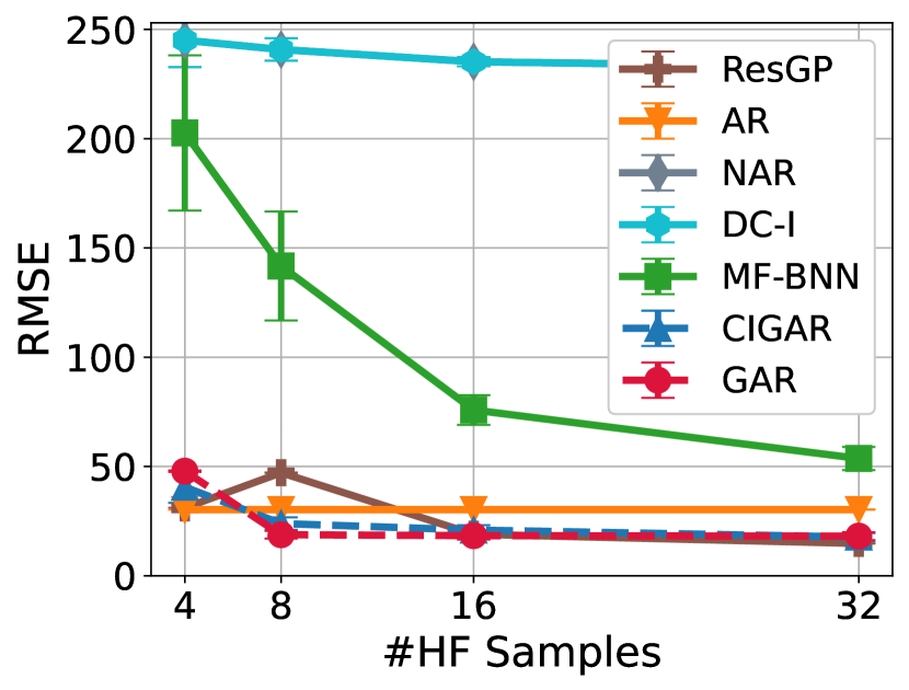
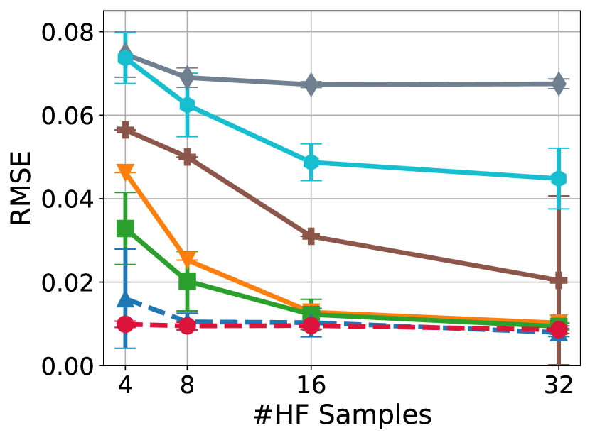
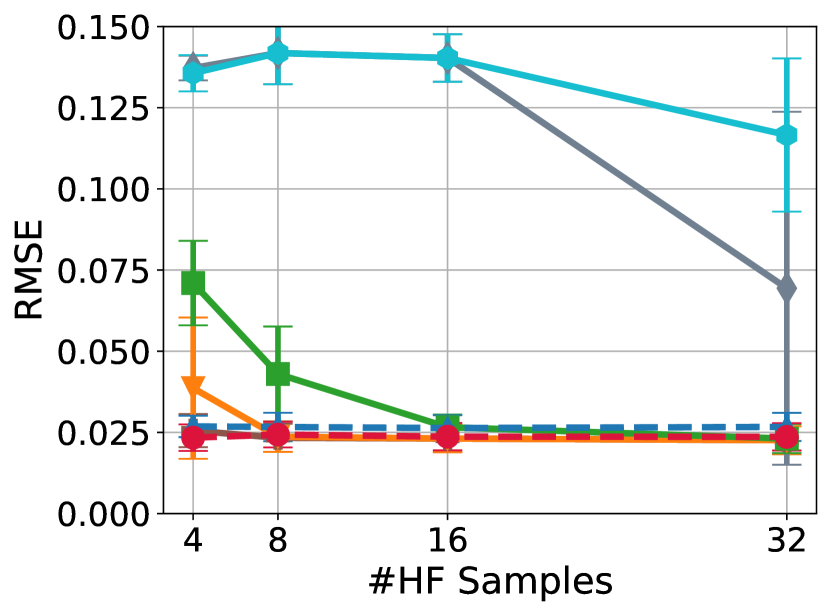
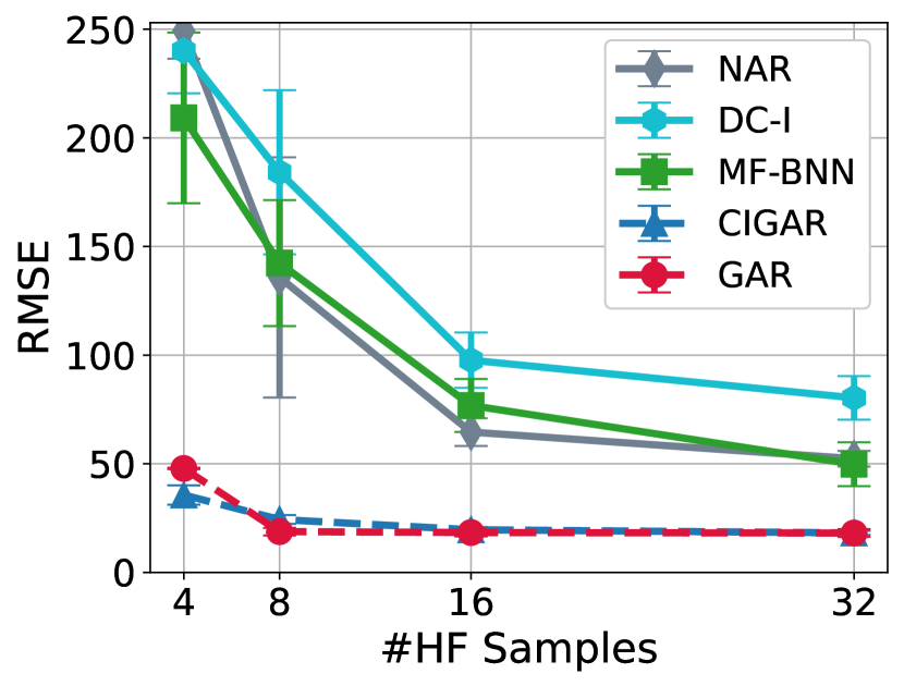
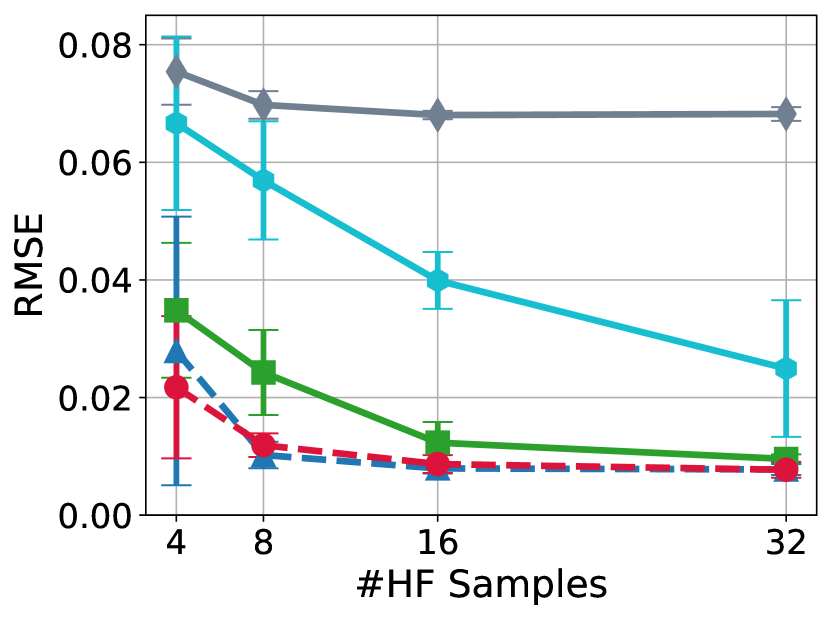
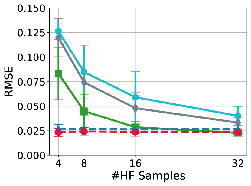
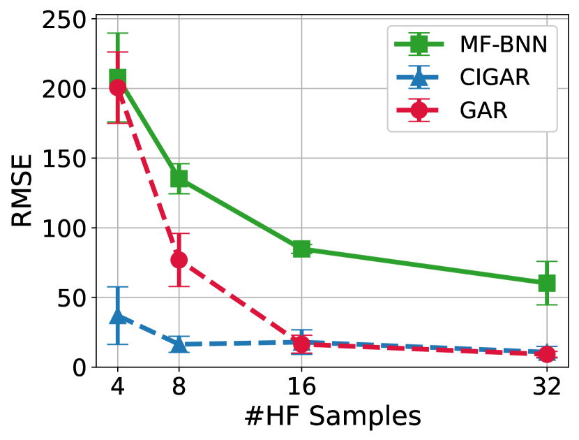
(a) Poisson’s equation

(b) Burger’s

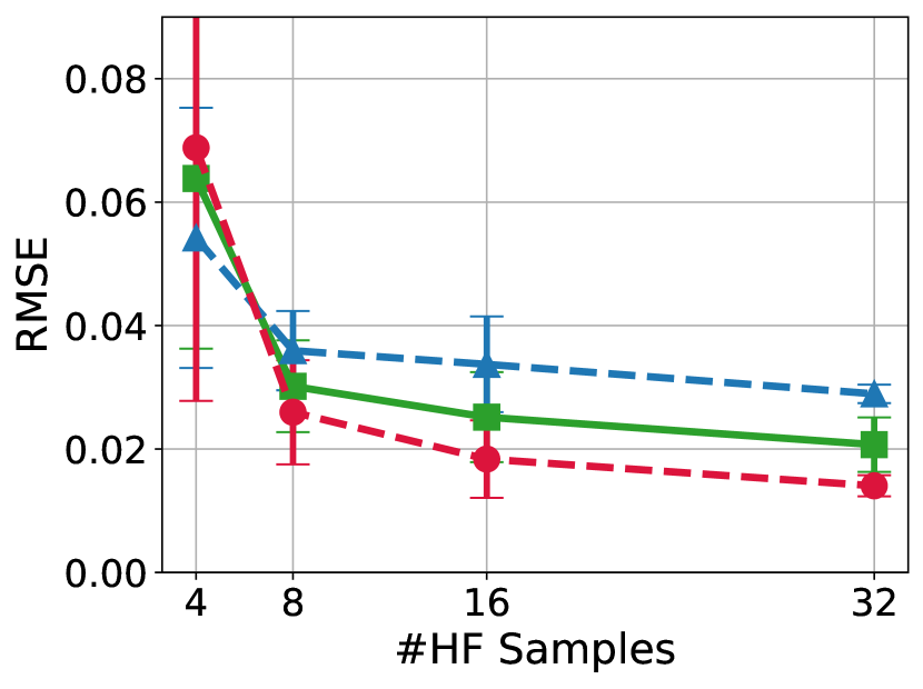
(c) Heat

Figure 1: RMSE against increasing number of high-fidelity training samples for Poisson’s, Burger’s, and heat equations with aligned outputs (top row), non-aligned outputs (middle row), and non-subset data (bottom row).

5.1 Multi-Fidelity Fusion for Canonical PDEs

We first assess GAR in canonical PDE simulation benchmarks, which produce high-dimensional spatial/spatial-temporal fields as model outputs. Specifically, we test on Burger’s, Poisson’s and the heat equations commonly used in the literature [12, 51, 52, 53]. The high fidelity results are obtained by solving these equations using finite difference on a $32\times 32$ mesh, whereas the low fidelity by an $8\times 8$ coarse mesh. The solutions on these grid points are recorded and vectorized as outputs. Because the mesh differs, the dimensionality varies. To compare with the standard multi-fidelity method that can only deal with aligned outputs, we use interpolation to upscale the low-fidelity and record them at the high-fidelity grid nodes. The corresponding inputs are PDE parameters and parameterized initial or boundary conditions. Detailed experimental setups can be found in Appendix E.1

We uniformly generate $128$ samples for testing and 32 for training. We increase the high-fidelity training samples to the number of low-fidelity training samples 32. The comparisons are conducted five times with shuffled samples. The statistical results (mean and std) of the RMSE are reported in Fig. 1. GAR and CIGAR outperform the competitors with a significant margin, up to 6x reduction in RMSE and also reaching the optimal performance with a maximum of 8 high-fidelity samples, indicating a successful fusion of low- and high-fidelity. CIGAR is slightly worse than GAR possibility due to the lack of hard constraints on the orthogonality of its weight matrixes during implementation. As we have discovered in the literature, AR consistently performs well. With a flexible linear transformation, GAR outperforms AR while inheriting its robustness, leading to the best performance. For the unaligned output, MF-BNN showed slightly worse performance than in the aligned cases, highlighting the challenges of the unaligned outputs. In contrast, GAR and CIGAR show almost identical performances for both cases. Nevertheless, MF-BNN also shows good performance compared to the rest of the other methods, which is consistent with the finding in [13]. It is interesting to see that for the non-subset data, the capable methods show better performances than in the subset cases. GAR and CIGAR still outperform the competitors with a clear margin.

To approximately assess the performance under an active learning process. We instead generate training samples in a Sobol sequence [54]. The results are shown in Appendix E.2 where GAR and CIGAR also outperform the other methods by a large margin.

5.2 Multi-Fidelity Fusion for Real-World Applications

Optimal topology structure is the optimized layout of materials, e.g., alloy and concrete, given some design specifications, e.g., external force and angle. This topology optimization is a key technique in mechanical designs, but it is also known for its high computational cost, which renders the need for multi-fidelity fusion. We consider the topology optimization of a cantilever beam with the location of the point load, the angle of the point load, and the filter radius [55] as system inputs. The low-fidelity use a $16\times 16$ regular mesh for the finite element solver, whereas the high-fidelity $64\times 64$. Please see Appendix E.3 for a detailed setup.

As in the previous experiment, the RMSE statistics against an increasing number of high-fidelity training samples are shown in Fig. 2. It is clear that GAR outperforms the competitors with a large margin consistently. CIGAR can be as good as GAR when the number of training samples is large.

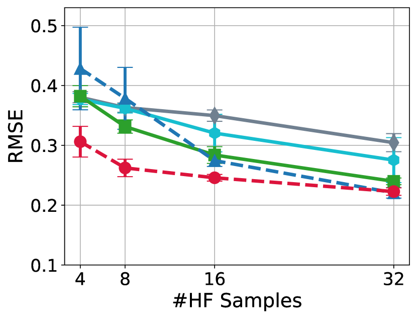
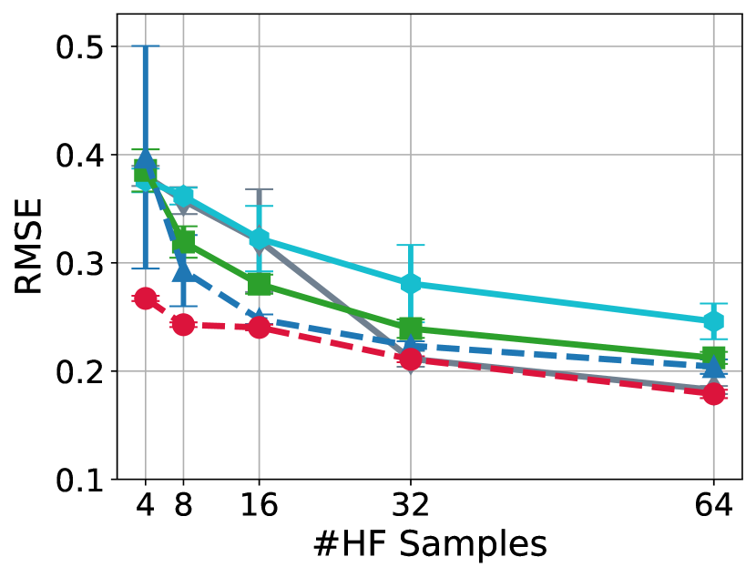
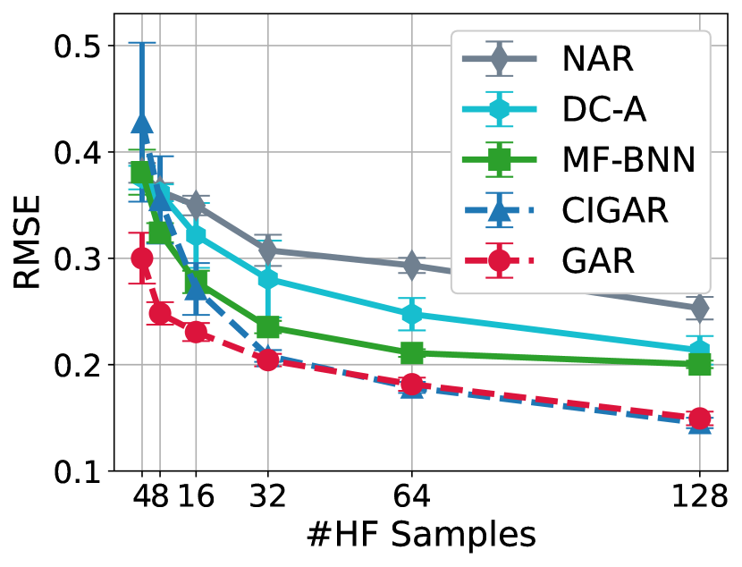
Figure 2: RMSE with low-fidelity training sample number fixed to {32,64,128}.

Steady-state 3D solid oxide fuel cell, which solves complex coupled PDEs including Ohm’s law, Navier-Stokes equations, Brinkman equation, Maxwell-Stefan diffusion, and convection simultaneously, is a key model for modern fuel cell optimization. The model was solved using finite elements in COMSOL. The inputs were taken to be the electrode porosities, cell voltage, temperature, and pressure in the channels. The low-fidelity experiment is conducted using 3164 elements and relative tolerance of 0.1, whereas the high-fidelity uses 37064 elements and relative tolerance of 0.001. The outputs are the coupled fields of electrolyte current density (ECD) and ionic potential (IP) in the $x-z$ plane located at the center of the channel.

The RMSE statistics are shown in Fig. 5(a), which, again, highlights the superiority of the proposed method with only four high-fidelity data training samples. To further assess the model capacity for non-structured outputs, we keep only the ECD (Fig. 5(b)) and IP (Fig. 5(c)) in the low-fidelity training data to rise the challenges of predicting high fidelity ECD+IP fields. We can see that removing some low-fidelity information indeed increases the difficulties, especially when removing ECD, where MF-BNN outperforms GAR and CIGAR with a small number of training data. As soon as the training number increases, GAR and CIGAR become superior again.

Plasmonic nanoparticle arrays is a complex physical simulation that calculates the extinction and scattering efficiencies $Q_{ext}$ and $Q_{sc}$ for plasmonic systems with varying numbers of scatterers using coupled dipole approximation (CDA), which is a method for mimicking the optical response of an array of similar, non-magnetic metallic nanoparticles with dimensions far smaller than the wavelength of light (here 25 nm). $Q_{ext}$ and $Q_{sc}$ are defined as the QoIs in this work. Please see Appendix E.5 for detailed experiment setup. We conducted the experiments 5 times with shuffled samples, and we fixed the number of low-fidelity training samples to 32, 64, and 128 and gradually increase the high-fidelity training data from 4 to 32, 64, and 128. We can see in Fig.3, GAR outperforms others by a clear margin, especially when the high-fidelity data contains only 4 samples. When there is a large training sample dataset, CIGAR can be as excellent as GAR.

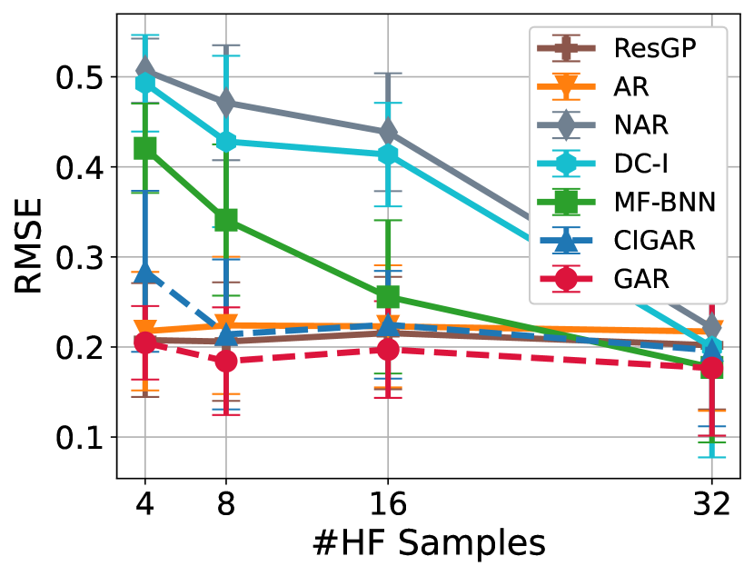
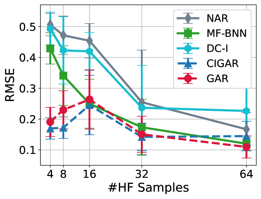
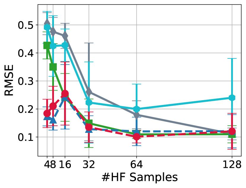
Figure 3: RMSE against an increasing number of high-fidelity training samples with low-fidelity training sample number fixed to {32,64,128} for Plasmonic nanoparticle arrays simulations.

5.3 Stability Test

As a non-parametric model, we expect GAR and CIGAR to have stable performance against overfitting compared to the NN-based methods. In this section, we show the testing RMSE against the training epoch for GAR, CIGAR, and MF-BNN for the previous Poisson’s equation, SOFC, and topology optimization. The experiments are repeated five times to ensure fairness. The results are shown in Fig. 4. We can see clearly that GAR and CIGAR are more stable than MF-BNN in almost all cases. The most notables are the converge rate of GAR and CIGAR, which is more than 10x faster if we look at the topology optimization and SOFC cases. For Poisson’s equation, the MF-BNN is not likely to match the performance of GAR and CIGAR regardless of the large number of training epochs being used. For the SOFC, MF-BNN, and topology optimization, MF-BNN might be able to match GAR given a very large epoch number, making it a bad choice that consumes expensive computational resources.

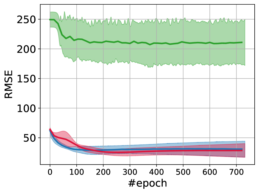
(a) Poisson’s

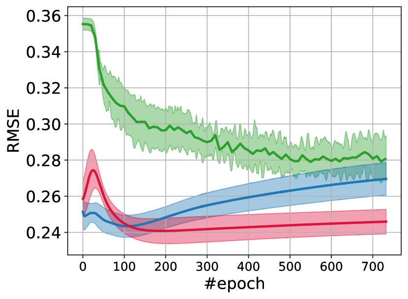
(b) Topology optimization

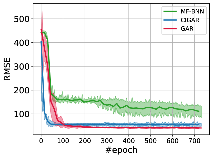
(c) SOFC

Figure 4: Testing RMSE against an increasing number of training epochs for SOFC, topology optimization, and Poisson datasets.

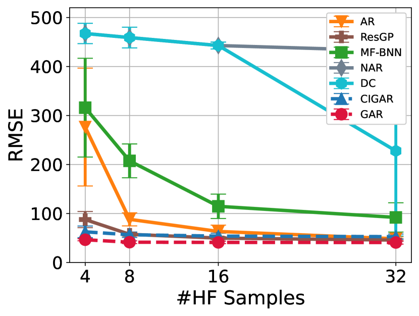
(a) ECD+IP

(b) ECD

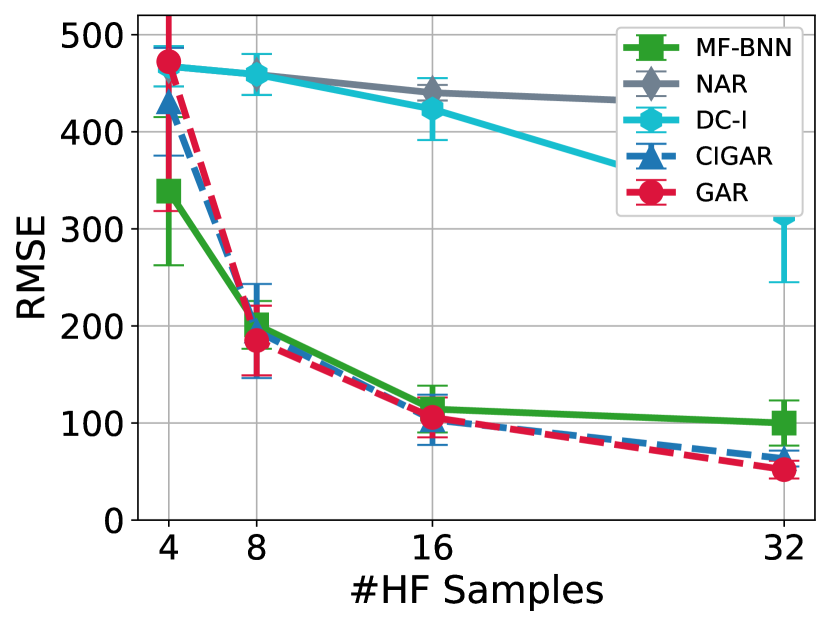
(c) IP

Figure 5: RMSE for SOFC with low-fidelity training sample number fixed to 32.

6 Conclusion

We propose GAR, the first AR generalization to arbitrary outputs and non-subset multi-fidelity data with a closed-form solution, and CIGAR, an efficient implementation by revealing the autokrigeability in AR. Limitation of this work is scalability w.r.t to samples, lack of active learning [13], and the applications to broader problems of time series and transfer learning[49, 50] using AR-based methods.

Checklist

The checklist follows the references. Please read the checklist guidelines carefully for information on how to answer these questions. For each question, change the default [TODO] to [Yes] , [No] , or [N/A] . You are strongly encouraged to include a justification to your answer, either by referencing the appropriate section of your paper or providing a brief inline description. For example:

• Did you include the license to the code and datasets? [Yes] See Section LABEL:gen_inst.

• Did you include the license to the code and datasets? [No] The code and the data are proprietary.

• Did you include the license to the code and datasets? [N/A]

Please do not modify the questions and only use the provided macros for your answers. Note that the Checklist section does not count towards the page limit. In your paper, please delete this instructions block and only keep the Checklist section heading above along with the questions/answers below.

1. For all authors…

   1. Do the main claims made in the abstract and introduction accurately reflect the paper’s contributions and scope? [Yes] See contributions, abstract, and introduction

   2. Did you describe the limitations of your work? [Yes] See the conclusion and complexity analysis section

   3. Did you discuss any potential negative societal impacts of your work? [N/A] We do not see an obvisou negative societal impacts as it is fundamental and quite theoretical.

   4. Have you read the ethics review guidelines and ensured that your paper conforms to them? [Yes]

2. If you are including theoretical results…

   1. Did you state the full set of assumptions of all theoretical results? [Yes]

   2. Did you include complete proofs of all theoretical results? [Yes] Please see Appendix

3. If you ran experiments…

   1. Did you include the code, data, and instructions needed to reproduce the main experimental results (either in the supplemental material or as a URL)? [Yes] Please see supplementary materials

   2. Did you specify all the training details (e.g., data splits, hyperparameters, how they were chosen)? [Yes] Please see the Appendix

   3. Did you report error bars (e.g., with respect to the random seed after running experiments multiple times)? [Yes] Please see the experimental section

   4. Did you include the total amount of compute and the type of resources used (e.g., type of GPUs, internal cluster, or cloud provider)? [Yes] Please see the experimental section

4. If you are using existing assets (e.g., code, data, models) or curating/releasing new assets…

   1. If your work uses existing assets, did you cite the creators? [Yes] Please see the experimental section

   2. Did you mention the license of the assets? [Yes]

   3. Did you include any new assets either in the supplemental material or as a URL? [Yes]

   4. Did you discuss whether and how consent was obtained from people whose data you’re using/curating? [Yes] see experiment senction and the Appendix

   5. Did you discuss whether the data you are using/curating contains personally identifiable information or offensive content? [N/A] We do not use such data

5. If you used crowdsourcing or conducted research with human subjects…

   1. Did you include the full text of instructions given to participants and screenshots, if applicable? [N/A]

   2. Did you describe any potential participant risks, with links to Institutional Review Board (IRB) approvals, if applicable? [N/A]

   3. Did you include the estimated hourly wage paid to participants and the total amount spent on participant compensation? [N/A]

 

Appendix

 

Appendix A Gaussian process

Gaussian process (GP) is a typical choice for the surrogate model because of its model capacity for complicated black-box functions and uncertainty quantification. Consider, for the time being, a simplified scenario in which we have noise-contaminated observations $\{y_{i}=g({{\bf x}}_{i})+\epsilon_{i}\}_{i=1}^{N}$. In a GP model, a prior distribution is placed over $f({{\bf x}})$, indexed by ${{\bf x}}$:

$$\eta({{\bf x}})|{\bm{\theta}}\sim\mathcal{GP}\left(m({{\bf x}}),k({{\bf x}},{{\bf x}}^{\prime}|{\bm{\theta}})\right),$$ (A.1)

with mean and covariance functions:

$$\begin{array}[]{ll}m_{0}({{\bf x}})&=\mathbb{E}[f({{\bf x}})],\\ k({{\bf x}},{{\bf x}}^{\prime}|\boldsymbol{\theta})&=\mathbb{E}[(f({{\bf x}})-m_{0}({{\bf x}}))(f({{\bf x}}^{\prime})-m_{0}({{\bf x}}^{\prime}))],\end{array}$$ (A.2)

where $\mathbb{E}[\cdot]$ is the expectation and $\boldsymbol{\theta}$ are the hyperparameters that control the kernel function. By centering the data, the mean function may be assumed to be an equal constant, $m_{0}({{\bf x}})\equiv m_{0}$. Alternative options are feasible, such as a linear function of ${{\bf x}}$, but they are rarely used until previous knowledge of the shape of the function is provided. The covariance function can take several forms, with the automated relevance determinant (ARD) kernel being the most popular.

$$k({{\bf x}},{{\bf x}}^{\prime}|\boldsymbol{\theta})=\theta_{0}\exp\left(-({{\bf x}}-{{\bf x}}^{\prime})^{T}\mbox{diag}(\theta_{1}^{-2},\ldots,\theta_{l}^{-2})({{\bf x}}-{{\bf x}}^{\prime})\right).$$ (A.3)

From this point on, we eliminate the explicit notation of $k(x,x^{\prime})$’s reliance on $\boldsymbol{\theta}$. In this instance, the hyperparameters $\theta_{1},\ldots,\theta_{l}$ are referred to as length-scales. For constant parameter ${{\bf x}}$, $f({{\bf x}})$ is its random variable. In contrast, a collection of values, $f({{\bf x}}_{i})$, $i=1,\ldots,N$, is a partial realization of the GP. GP’s realizations are functions of $x$ that are deterministic. The primary characteristic of GPs is that the joint distribution of $eta(xi),i=1,hdots,N$ is multivariate Gaussian.

Assuming the model deficiency $\varepsilon\sim\mathcal{N}(0,\sigma^{2})$ is likewise Gaussian, we can derive the model likelihood using the prior (A.1) and available data.

$$\mathcal{L} \triangleq p({\bf y}|{\bf x},\bm{\theta})=\int(f({\bf x})+\varepsilon)df=\mathcal{N}({\bf y}|m_{0}\bm{1},\textbf{K}+\sigma^{2}{\bf I})$$ (A.4)

$$=-\frac{1}{2}\left({{\bf y}}-{m_{0}}{\bf 1}\right)^{T}(\textbf{K}+\sigma^{2}{\bf I})^{-1}\left({{\bf y}}-{m_{0}}{\bf 1}\right)$$

$$\quad-\frac{1}{2}\ln|\textbf{K}+\sigma^{2}{\bf I}|-\frac{N}{2}\log(2\pi),$$

where ${\bf K}=[K_{ij}]$ is the covariance matrix, in which $K_{ij}=k({{\bf x}}_{i},{{\bf x}}_{j})$, $i,j=1,\ldots,N$. The hyperparameters $\boldsymbol{\theta}$ is often derived from point estimations using the maximum likelihood (MLE) of Eq. (A.4) w.r.t. $\bm{\theta}$. The joint distribution of ${\bf y}$ and $f({\bf x})$ is also a joint Gaussian distribution with mean value $m_{0}\bm{1}$ and covariance matrix.

$$\begin{array}[]{c}\displaystyle\textbf{K}^{\prime}=\left[\begin{array}[]{c|c}\textbf{K}+\sigma^{2}{\bf I}&{{\bf k}}({{\bf x}})\\ \hline\cr{{\bf k}}^{T}({{\bf x}})&k({{\bf x}},{{\bf x}})+\sigma^{2}\end{array}\right],\end{array}$$ (A.5)

where ${{\bf k}}({{\bf x}})=(k({{\bf x}}_{1},{{\bf x}}),\ldots,k({{\bf x}}_{N},{{\bf x}}))^{T}$. Conditioning on ${\bf y}$, the conditional predictive distribution at ${\bf x}$ is obtained.

$$\begin{array}[]{c}\hat{f}({{\bf x}})|{{\bf y}}\sim\mathcal{N}\left(\mu({{\bf x}}),v({{\bf x}},{{\bf x}}^{\prime})\right),\vspace{2mm}\\ \mu({{\bf x}})=m_{0}{\bf 1}+{{\bf k}}({{\bf x}})^{T}\left(\textbf{K}+\sigma^{2}{\bf I}\right)^{-1}\left({\bf y}-{m_{0}}{\bf 1}\right),\vspace{2mm}\\ v({{\bf x}})=\sigma^{2}+k({{\bf x}},{{\bf x}})-{{\bf k}}^{T}({{\bf x}})\left(\textbf{K}+\sigma^{2}{\bf I}\right)^{-1}{{\bf k}}({{\bf x}}).\end{array}$$ (A.6)

The expected value $\mathbb{E}[f({{\bf x}})]$ is given by $\mu({{\bf x}})$ and the predictive variance by $v({{\bf x}})$. From Eq. (A.5) to Eq. (A.6) is crucial since the prediction posterior of this wake is based on a comparable block covariance matrix.

Appendix B Proof of Theorem

Lemma 1.

[16] If ${\bf X}^{h}\subset{\bf X}^{l}$, the joint likelihood of AR can be decomposed into two independent likelihoods of the low- and high-fidelity.

This lemma has been proven by [15]. However, the notation and derivation is not easy to follow. To layout the foundations of GAR, we prove it using a clearer way with friendly notations.

Proof.

Following Eq. (2), the inversion of the covariance matrix is

$$\bm{\Sigma}^{-1}=\left(\begin{array}[]{cc}{({\bf K}^{l})^{-1}+\left(\begin{array}[]{cc}{0}&{0}\\ {0}&\rho^{2}({\bf K}^{r})^{-1}\end{array}\right)}&{-\left(\begin{array}[]{c}{0}\\ \rho({\bf K}^{r})^{-1}\end{array}\right)}\\ {-\left({0}\quad\rho({\bf K}^{r})^{-1}\right)}&{({\bf K}^{r})^{-1}}\end{array}\right).$$

We can write down the log-likelihood for all the low- and high-fidelity observations as,

$$\log p({{\bf Y}}^{l},{{\bf Y}}^{h})$$ (A.7)

$$= -\frac{N^{h}+N^{l}}{2}\log(2\pi)-\frac{1}{2}\log|\bm{\Sigma}|-\frac{1}{2}({{\bf Y}}^{l},\rho{\bf E}^{T}{{\bf Y}}^{l}+{{\bf Y}}^{r})^{T}\bm{\Sigma}^{-1}\left(\begin{array}[]{c}{{\bf Y}}^{l}\\ \rho{\bf E}^{T}{{\bf Y}}^{l}+{{\bf Y}}^{r}\end{array}\right)$$

$$= -\frac{1}{2}\log|\bm{\Sigma}|-\frac{N^{h}+N^{l}}{2}\log(2\pi)-\frac{1}{2}[({{\bf Y}}^{l})^{T}({\bf K}^{l})^{-1}{\bf Y}^{l}+({{\bf Y}}^{l})^{T}\left(\begin{array}[]{cc}{\bf 0}&{\bf 0}\\ {\bf 0}&\rho^{2}{({\bf K}^{r})}^{-1}\end{array}\right){\bf Y}^{l}$$

$$-\rho({{\bf Y}}^{l})^{T}{\bf E}{\left({0},\ \rho({\bf K}^{r})^{-1}\right)}{\bf Y}^{l}-{\left({0},\ ({\bf Y}^{r})^{T}\rho({\bf K}^{r})^{-1}\right)}{\bf Y}^{l}-({{\bf Y}}^{l})^{T}{\bf E}\rho{{\bf K}_{r}}^{-1}(\rho{\bf E}^{T}{{\bf Y}}^{l}+{{\bf Y}}^{r})$$

$$+\rho{\bf Y}^{l}{\bf E}({\bf K}^{r})^{-1}(\rho{\bf E}^{T}{{\bf Y}}^{l}+{{\bf Y}}^{r})+{\bf Y}^{r}({\bf K}^{r})^{-1}(\rho{\bf E}^{T}{{\bf Y}}^{l}+{{\bf Y}}^{r})]$$

$$= -\frac{1}{2}\log|\bm{\Sigma}|-\frac{N^{h}+N^{l}}{2}\log(2\pi)-\frac{1}{2}[({{\bf Y}}^{l})^{T}({\bf K}^{l})^{-1}{\bf Y}^{l}-{\left({0},\ ({\bf Y}^{r})^{T}\rho({\bf K}^{r})^{-1}\right)}{\bf Y}^{l}$$

$$+{\bf Y}^{r}({\bf K}^{r})^{-1}\rho{\bf E}^{T}{{\bf Y}}^{l}+{\bf Y}^{r}({\bf K}^{r})^{-1}{{\bf Y}}^{r}]$$

$$= -\frac{1}{2}\log|{\bf K}^{l}|-\frac{1}{2}\log|{\bf K}^{r}|-\frac{N^{l}+N^{h}}{2}log(2\pi)-\frac{1}{2}({{\bf Y}}^{l})^{T}({\bf K}^{l})^{-1}{\bf Y}^{l}-\frac{1}{2}{\bf Y}^{r}({\bf K}^{r})^{-1}{{\bf Y}}^{r}$$

$$= \underbrace{-\frac{N^{L}}{2}log(2\pi)-\frac{1}{2}\log|{\bf K}^{l}|-\frac{1}{2}({{\bf Y}}^{l})^{T}({\bf K}^{l})^{-1}{{\bf Y}}^{l}}_{\mathcal{L}^{l}}\underbrace{-\frac{N^{h}}{2}log(2\pi)-\frac{1}{2}\log|{\bf K}^{r}|-\frac{1}{2}({{\bf Y}}^{r})^{T}({\bf K}^{r})^{-1}{{\bf Y}}^{r}}_{\mathcal{L}^{r}}$$

∎

where ${\bf Y}^{r}={\bf Y}^{h}-\rho{\bf E}^{T}{\bf Y}^{l}$, ${\mathcal{L}^{l}}$ is the log-likelihood of the low-fidelity data with the lower fidelity kernel, and ${\mathcal{L}^{r}}$ is the log-likelihood of the residual data with the residual kernel; ${\mathcal{L}^{l}}$ and ${\mathcal{L}^{r}}$ are independent and thus can be trained in parallel.

Based on the joint probability Eq. (2), we can similarly derive the predictive posterior distribution of the high-fidelity using the standard GP posterior derivation. Conditioning on ${\bf Y}^{h}$ and ${\bf Y}^{l}$, the predictive high-fidelity posterior for a new input ${\bf x}_{*}$ is also a Gaussian ${\mathcal{N}}({\mu}_{*}^{h},\sigma^{h}_{*})$:

$${\mu^{h}_{*}}= \left(\rho{\bf k}^{l}({\bf x}_{*},{\bf X}^{l}),\ \ \rho^{2}{\bf k}^{l}({\bf x}_{*},{\bf X}^{h})+{\bf k}^{r}({\bf x}_{*},{\bf X}^{h})\right){\bf K}^{-1}\left(\begin{array}[]{c}{{\bf Y}}^{l}\\ \rho{\bf E}^{T}{{\bf Y}}^{l}+{{\bf Y}}^{r}\end{array}\right)$$ (A.8)

$$= \rho{\bf k}^{l}({\bf x}_{*},{\bf X}^{l}){\bf K}^{l}({\bf X}^{l},{\bf X}^{l})^{-1}{{\bf Y}}^{l}$$

$$+\rho^{3}{\bf k}^{l}({\bf x}_{*},{\bf X}^{l}){\bf E}({\bf K}^{r})^{-1}{\bf E}^{T}{{\bf Y}}^{l}-\rho^{3}{\bf k}^{l}({\bf x}_{*},{\bf X}^{h})({\bf K}^{r})^{-1}{\bf E}^{T}{{\bf Y}}^{l}$$

$$-\rho{\bf k}^{r}({\bf x}_{*},{\bf X}^{h})({\bf K}^{r})^{-1}{\bf E}^{T}{{\bf Y}}^{l}-\rho^{2}{\bf k}^{l}({\bf x}_{*},{\bf X}^{l}){\bf E}({\bf K}^{r})^{-1}\left[\rho{\bf E}^{T}{{\bf Y}}^{l}+{{\bf Y}}^{r}\right]$$

$$+\rho^{2}{\bf k}^{l}({\bf x}_{*},{\bf X}^{h})({\bf K}^{r})^{-1}\left[\rho{\bf E}^{T}{{\bf Y}}^{l}+{{\bf Y}}^{r}\right]+{\bf k}^{r}({\bf x}_{*},{\bf X}^{h})({\bf K}^{r})^{-1}\left[\rho{\bf E}^{T}{{\bf Y}}^{l}+{{\bf Y}}^{r}\right]$$

$$= \left[\rho{\bf k}^{l}({\bf x}_{*},{\bf X}^{l})({\bf K}^{l})^{-1}\right]{{\bf Y}}^{l}+{\bf k}^{r}({\bf x}_{*},{\bf X}^{h})({\bf K}^{r})^{-1}{{\bf Y}}^{r}$$

$$-\left[\rho{\bf k}^{r}({\bf x}_{*},{\bf X}^{h})({\bf K}^{r})^{-1}\right]{\bf E}{{\bf Y}}^{l}+\left[\rho{\bf k}^{r}({\bf x}_{*},{\bf X}^{h})({\bf K}^{r})^{-1}\right]{\bf E}{{\bf Y}}^{l}$$

$$= \left[\rho{\bf k}^{l}({\bf x}_{*},{\bf X}^{l})({\bf K}^{l})^{-1}\right]{{\bf Y}}^{l}+{\bf k}^{r}({\bf x}_{*},{\bf X}^{h})({\bf K}^{r})^{-1}{{\bf Y}}^{r}$$

and

$${\sigma_{*}^{h}}= \left(\rho^{2}{\bf k}^{l}({\bf x}_{*},{\bf x}_{*})+{\bf k}^{r}({\bf x}_{*},{\bf x}_{*})\right)-(\rho{\bf k}_{*}^{l},\rho^{2}{\bf k}_{*}^{l}({\bf X}^{h})+{\bf k}_{*}^{r})^{T}{\bf K}^{-1}(\rho{\bf k}_{*}^{l},\rho^{2}{\bf k}_{*}^{l}({\bf X}^{h})+{\bf k}_{*}^{r})$$ (A.9)

$$= \left(\rho^{2}{\bf k}^{l}({\bf x}_{*},x_{*})+{\bf k}^{r}({\bf x}_{*},{\bf x}_{*})\right)-\left(\rho({\bf k}^{l}_{*})^{T}({\bf K}^{l})^{-1}\rho{\bf k}^{l}_{*}\right)+\left({\bf 0},\rho({\bf k}^{r}_{*})^{T}({\bf K}^{r})^{-1}\right)\rho{\bf k}^{l}_{*}$$

$$-({\bf k}^{r}_{*})^{T}({\bf K}^{r})^{-1}\rho^{2}{\bf k}^{l}_{*}({\bf X}^{h})-({\bf k}^{r}_{*})^{T}({\bf K}^{r})^{-1}{\bf k}_{*}^{r}$$

$$= \rho^{2}\left({\bf k}^{l}({\bf x}_{*},{\bf x}_{*})-({\bf k}^{l}_{*})^{T}({\bf K}^{l})^{-1}{\bf k}^{l}_{*}\right)+\left({\bf k}^{r}({\bf x}_{*},{\bf x}_{*})-({\bf k}^{r}_{*})^{T}({\bf K}^{r})^{-1}{\bf k}^{r}_{*}\right)$$

where, ${\bf k}_{*}^{l}({\bf X}^{h})={\bf k}^{l}({\bf x}_{*},{\bf X}^{h})$ is the covariance vector between the new inputs ${\bf x}_{*}$ and ${\bf X}^{h}$. Notice that the predictive posterior is also decomposed into two independent parts that related to the low-fidelity GP and the residual GP, which is convenient for parallel computing and saving computational resources.

Lemma 2.

Given tensor GP priors for ${\bm{\mathsfit{Y}}}^{l}({\bf x},{\bf x}^{\prime})$ and ${\bm{\mathsfit{Y}}}^{r}({\bf x},{\bf x}^{\prime})$ and the Tucker transformation of Eq. (3), the joint probability for ${\bf y}=[\mathrm{vec}({{\bm{\mathsfit{Y}}}^{l}})^{T},\mathrm{vec}({\bm{\mathsfit{Y}}}^{h})^{T}]^{T}$ is ${\bf y}\sim{\mathcal{N}}({\bf 0},\bm{\Sigma})$, where $\bm{\Sigma}=$
$\left(\begin{array}[]{cc}{\bf K}^{l}({\bf X}^{l},{\bf X}^{l})\otimes\left(\bigotimes_{m=1}^{M}{\bf S}^{l}_{m}\right)&{\bf K}^{l}({\bf X}^{l},{\bf X}^{h})\otimes\left(\bigotimes_{m=1}^{M}{\bf S}^{l}_{m}{\bf W}_{m}^{T}\right)\\ {\bf K}^{l}({\bf X}^{h},{\bf X}^{l})\otimes\left(\bigotimes_{m=1}^{M}{\bf W}_{m}{\bf S}^{l}_{m}\right)&{\bf K}^{l}({\bf X}^{h},{\bf X}^{h})\otimes\left(\bigotimes_{m=1}^{M}{\bf W}_{m}{\bf S}^{l}_{m}{\bf W}_{m}\right)+{\bf K}^{r}({\bf X}^{h},{\bf X}^{h})\otimes\left(\bigotimes_{m=1}^{M}{\bf S}^{r}_{m}\right)\end{array}\right)$

Proof.

Since the $\bm{\Sigma}$ is the covariance matrix of ${\bf y}$, it can be expressed in block form as:

$$\bm{\Sigma}=\left(\begin{array}[]{cc}\mathrm{cov}(\mathrm{vec}({\bm{\mathsfit{Y}}}^{l}),\mathrm{vec}({\bm{\mathsfit{Y}}}^{l}))&\mathrm{cov}(\mathrm{vec}({\bm{\mathsfit{Y}}}^{l}),\mathrm{vec}({\bm{\mathsfit{Y}}}^{h}))\\ \mathrm{cov}(\mathrm{vec}({\bm{\mathsfit{Y}}}^{h}),\mathrm{vec}({\bm{\mathsfit{Y}}}^{l}))&\mathrm{cov}(\mathrm{vec}({\bm{\mathsfit{Y}}}^{h}),\mathrm{vec}({\bm{\mathsfit{Y}}}^{h}))\end{array}\right),$$

where $\mathrm{cov}(\mathrm{vec}({\bm{\mathsfit{Y}}}^{l}),\mathrm{vec}({\bm{\mathsfit{Y}}}^{h}))=\mathrm{cov}(\mathrm{vec}({\bm{\mathsfit{Y}}}^{l}),\mathrm{vec}({\bm{\mathsfit{Y}}}^{h}))^{T}$ is the cross covariance between ${\bm{\mathsfit{Y}}}^{l}$ and ${\bm{\mathsfit{Y}}}^{h}$. Assuming ${\bm{\mathsfit{Y}}}^{h}\in\mathbb{R}^{N^{h}\times d^{h}_{1}\times...\times d^{h}_{M}}$ and ${\bm{\mathsfit{Y}}}^{l}\in\mathbb{R}^{N^{l}\times d^{l}_{1}\times...\times d^{l}_{M}}$, together with the property of the Tucker operator in Eq. (3), the high-fidelity data and low-fidelity data have the following transformation,

$${{\bm{\mathsfit{Y}}}^{h}} ={\bm{\mathsfit{Y}}}^{l}\times_{1}{\bf E}\times_{2}{\bf W}_{1}\times_{3}...\times_{M}{\bf W}_{M-1}\times_{M+1}{\bf W}_{M}$$ (A.10)

$$\mathrm{vec}({{\bm{\mathsfit{Y}}}^{h}}) =\left[{\bf E}\otimes\left(\bigotimes_{m=1}^{M}{\bf W}_{m}\right)\right]\mathrm{vec}({{\bm{\mathsfit{Y}}}^{l}})+\mathrm{vec}({{\bm{\mathsfit{Y}}}^{r}}),$$

where $\forall i=1,2,...,M,{\bf W}_{i}\in\mathbb{R}^{d^{h}_{i}\times d^{l}_{i}}$, and ${\bf E}^{T}=\left({\bf 0},{\bf I}_{N^{h}}\right)\in\mathbb{R}^{N^{h}\times N^{l}}$ is the selection matrix such that ${\bf X}^{h}={\bf E}^{T}{\bf X}^{l}$. By definition our GP prior, the low-fidelity data has the joint probability:

$$\mathrm{vec}({{\bm{\mathsfit{Y}}}^{l}})\sim{\mathcal{N}}\left(0,{\bf K}^{l}({\bf X}^{l},{\bf X}^{l})\otimes\left(\bigotimes_{m=1}^{M}{\bf S}^{l}_{m}\right)\right)$$

Thus the covariance matrix of low-fidelity data is $\mathrm{cov}(\mathrm{vec}({\bm{\mathsfit{Y}}}^{l}),\mathrm{vec}({\bm{\mathsfit{Y}}}^{l}))={\bf K}^{l}({\bf X}^{l},{\bf X}^{l})\otimes\left(\bigotimes_{m=1}^{M}{\bf S}^{l}_{m}\right)$. After that, we can derive the other part of the $\bm{\Sigma}$. Firstly, assuming the residual information $\mathrm{vec}({\bm{\mathsfit{Y}}}^{r})$ is independent from $\mathrm{vec}({\bm{\mathsfit{Y}}}^{l})$, the covariance between $\mathrm{vec}({\bm{\mathsfit{Y}}}^{h})$ and $\mathrm{vec}({\bm{\mathsfit{Y}}}^{l})$ is

$$\mathrm{cov}(\mathrm{vec}({\bm{\mathsfit{Y}}}^{l}),\mathrm{vec}({\bm{\mathsfit{Y}}}^{h}))= \mathrm{cov}\left(\mathrm{vec}({\bm{\mathsfit{Y}}}^{l}),\left[{\bf E}\otimes\left(\bigotimes_{m=1}^{M}{\bf W}_{m}\right)\right]\mathrm{vec}({{\bm{\mathsfit{Y}}}^{l}})+\mathrm{vec}({{\bm{\mathsfit{Y}}}^{r}})\right)$$ (A.11)

$$= \mathrm{cov}\left(\mathrm{vec}({{\bm{\mathsfit{Y}}}^{l}}),\mathrm{vec}({\bm{\mathsfit{Y}}}^{r})\right)+\mathrm{cov}\left(\mathrm{vec}({\bm{\mathsfit{Y}}}^{l}),\left[{\bf E}\otimes\left(\bigotimes_{m=1}^{M}{\bf W}_{m}\right)\right]\mathrm{vec}({{\bm{\mathsfit{Y}}}}^{l})\right)$$

$$= \mathrm{cov}(\mathrm{vec}({{\bm{\mathsfit{Y}}}}^{l}),\mathrm{vec}({{\bm{\mathsfit{Y}}}^{l}}))\left[{\bf E}\otimes\left(\bigotimes_{m=1}^{M}{\bf W}_{m}\right)\right]^{T}$$

$$= \left[{\bf K}^{l}({\bf X}^{l},{\bf X}^{l})\otimes\left(\bigotimes_{m=1}^{M}{\bf S}^{l}_{m}\right)\right]\left[{\bf E}^{T}\otimes\left(\bigotimes_{m=1}^{M}{\bf W}_{m}^{T}\right)\right]$$

$$= {\bf K}^{l}({\bf X}^{l},{\bf X}^{h})\otimes\left(\bigotimes_{m=1}^{M}{\bf S}^{l}_{m}{\bf W}_{m}^{T}\right).$$

Since $\mathrm{cov}(\mathrm{vec}({\bm{\mathsfit{Y}}}^{l}),\mathrm{vec}({\bm{\mathsfit{Y}}}^{h}))$ is the transpose of $\mathrm{cov}(\mathrm{vec}({\bm{\mathsfit{Y}}}^{h}),\mathrm{vec}({\bm{\mathsfit{Y}}}^{l}))$, so the upper right part of $\bm{\Sigma}$ is

$$\mathrm{cov}(\mathrm{vec}({\bm{\mathsfit{Y}}}^{h}),\mathrm{vec}({\bm{\mathsfit{Y}}}^{l}))=\mathrm{cov}(\mathrm{vec}({\bm{\mathsfit{Y}}}^{l}),\mathrm{vec}({\bm{\mathsfit{Y}}}^{h}))^{T}= {\bf K}^{l}({\bf X}^{h},{\bf X}^{l})\otimes\left(\bigotimes_{m=1}^{M}{\bf W}_{m}{\bf S}^{l}_{m}\right).$$ (A.12)

For the lower and right part of $\bm{\Sigma}$, the covariance between $\mathrm{cov}(\mathrm{vec}({\bm{\mathsfit{Y}}}^{h}),\mathrm{vec}({\bm{\mathsfit{Y}}}^{h}))$ is

$$\mathrm{cov}(\mathrm{vec}({\bm{\mathsfit{Y}}}^{h}),\mathrm{vec}({\bm{\mathsfit{Y}}}^{h}))$$ (A.13)

$$= \mathrm{cov}\left(\left[{\bf E}\otimes\left(\bigotimes_{m=1}^{M}{\bf W}_{m}\right)\right]\mathrm{vec}({{\bm{\mathsfit{Y}}}^{l}})+\mathrm{vec}({{\bm{\mathsfit{Y}}}^{r}}),\left[{\bf E}\otimes\left(\bigotimes_{m=1}^{M}{\bf W}_{m}\right)\right]\mathrm{vec}({{\bm{\mathsfit{Y}}}^{l}})+\mathrm{vec}({{\bm{\mathsfit{Y}}}^{r}})\right)$$

$$= \mathrm{cov}\left(\left[{\bf E}\otimes\left(\bigotimes_{m=1}^{M}{\bf W}_{m}\right)\right]\mathrm{vec}({{\bm{\mathsfit{Y}}}^{l}}),\left[{\bf E}\otimes\left(\bigotimes_{m=1}^{M}{\bf W}_{m}\right)\right]\mathrm{vec}({{\bm{\mathsfit{Y}}}^{l}})\right)+\mathrm{cov}\left(\mathrm{vec}({\bm{\mathsfit{Y}}}^{r}),\mathrm{vec}({\bm{\mathsfit{Y}}}^{r})\right)$$

$$+\mathrm{cov}\left(\left[{\bf E}\otimes\left(\bigotimes_{m=1}^{M}{\bf W}_{m}\right)\right]\mathrm{vec}({{\bm{\mathsfit{Y}}}^{l}}),\mathrm{vec}({\bm{\mathsfit{Y}}}^{r})\right)+\mathrm{cov}\left(\mathrm{vec}({\bm{\mathsfit{Y}}}^{r}),\left[{\bf E}\otimes\left(\bigotimes_{m=1}^{M}{\bf W}_{m}\right)\right]\mathrm{vec}({{\bm{\mathsfit{Y}}}^{l}})\right)$$

$$= \left[{\bf E}\otimes\left(\bigotimes_{m=1}^{M}{\bf W}_{m}\right)\right]\left(\mathrm{cov}(\mathrm{vec}({{\bm{\mathsfit{Y}}}}^{l}),\mathrm{vec}({{\bm{\mathsfit{Y}}}^{l}}))\right)\left[{\bf E}\otimes\left(\bigotimes_{m=1}^{M}{\bf W}_{m}\right)\right]^{T}+\mathrm{cov}\left(\mathrm{vec}({{\bm{\mathsfit{Y}}}}^{r}),\mathrm{vec}({{\bm{\mathsfit{Y}}}}^{r})\right)$$

$$= {\bf K}^{l}({\bf X}^{h},{\bf X}^{h})\otimes\left(\bigotimes_{m=1}^{M}{\bf W}_{m}{\bf S}^{l}_{m}{\bf W}_{m}^{T}\right)+{\bf K}^{r}({\bf X}^{h},{\bf X}^{h})\left(\bigotimes_{m=1}^{M}{\bf S}^{r}_{m}\right).$$

Assembling the several parts together, we have the joint covariance matrix $\bm{\Sigma}$:

$$\left(\begin{array}[]{cc}{\bf K}^{l}({\bf X}^{l},{\bf X}^{l})\otimes\left(\bigotimes_{m=1}^{M}{\bf S}^{l}_{m}\right)&{\bf K}^{l}({\bf X}^{l},{\bf X}^{h})\otimes\left(\bigotimes_{m=1}^{M}{\bf S}^{l}_{m}{\bf W}_{m}^{T}\right)\\ {\bf K}^{l}({\bf X}^{h},{\bf X}^{l})\otimes\left(\bigotimes_{m=1}^{M}{\bf W}_{m}{\bf S}^{l}_{m}\right)&{\bf K}^{l}({\bf X}^{h},{\bf X}^{h})\otimes\left(\bigotimes_{m=1}^{M}{\bf W}_{m}{\bf S}^{l}_{m}{\bf W}_{m}\right)+{\bf K}^{r}({\bf X}^{h},{\bf X}^{h})\otimes\left(\bigotimes_{m=1}^{M}{\bf S}^{r}_{m}\right)\end{array}\right)$$ (A.14)

∎

Before we move on to the next proof, we introduce the matrix inversion property, which will become handy later.

Property 1.

For any invertible block matrixes $\left(\begin{array}[]{cc}{\bf A}&{\bf B}\\ {\bf B}^{T}&{\bf C}\end{array}\right)$, where the sub-matrixes are also invertible, we have $({\bf B}^{T},{\bf C})\left(\begin{array}[]{cc}{\bf A}&{\bf B}\\ {\bf B}^{T}&{\bf C}\end{array}\right)^{-1}=({\bf 0},{\bf I})$ and $\left(\begin{array}[]{cc}{\bf A}&{\bf B}\\ {\bf B}^{T}&{\bf C}\end{array}\right)^{-1}\left(\begin{array}[]{c}{\bf B}\\ {\bf C}\end{array}\right)=\left(\begin{array}[]{c}{\bf 0}\\ {\bf I}\end{array}\right)$.

Proof.

The inversion of a block matrix (if it is invertible) following the Sherman-Morrison formula is

$$\left(\begin{array}[]{cc}{\bf A}&{\bf B}\\ {\bf B}^{T}&{\bf C}\end{array}\right)^{-1}=\left(\begin{array}[]{cc}\bf P^{-1}&-\bf P^{-1}{\bf B}{\bf C}^{-1}\\ -{\bf C}^{-1}{\bf B}^{T}\bf P^{-1}&{\bf C}^{-1}+{\bf C}^{-1}{\bf B}^{T}\bf P^{-1}{\bf B}{\bf C}^{-1}\end{array}\right),a$$ (A.15)

where ${\bf P}={\bf A}-{\bf B}{\bf C}^{-1}{\bf B}^{T}$, we can then derive the multiplication in Property 1 by the rule of block matrix multiplication:

$$({\bf B}^{T},{\bf C})\left(\begin{array}[]{cc}{\bf A}&{\bf B}\\ {\bf B}^{T}&{\bf C}\end{array}\right)^{-1}$$ (A.16)

$$= ({\bf B}^{T},{\bf C})\left(\begin{array}[]{cc}\bf P^{-1}&-\bf P^{-1}{\bf B}{\bf C}^{-1}\\ -{\bf C}^{-1}{\bf B}^{T}\bf P^{-1}&{\bf C}^{-1}+{\bf C}^{-1}{\bf B}^{T}\bf P^{-1}{\bf B}{\bf C}^{-1}\end{array}\right)$$

$$= \left({\bf B}^{T}\bf P^{-1}-{\bf C}({\bf C}^{-1}{\bf B}^{T}\bf P^{-1}),-{\bf B}^{T}\bf P^{-1}{\bf B}{\bf C}^{-1}+{\bf C}{\bf C}^{-1}+{\bf C}({\bf C}^{-1}{\bf B}^{T}\bf P^{-1}{\bf B}{\bf C}^{-1})\right)$$

$$= \left({\bf B}^{T}\bf P^{-1}-{\bf B}^{T}\bf P^{-1},-{\bf B}^{T}\bf P^{-1}{\bf B}{\bf C}^{-1}+{\bf I}+{\bf B}^{T}\bf P^{-1}{\bf B}{\bf C}^{-1}\right)$$

$$= \left({\bf 0},{\bf I}\right).$$

Similarly, the other part of the conclusion can also be derived

$$\left(\begin{array}[]{cc}{\bf A}&{\bf B}\\ {\bf B}^{T}&{\bf C}\end{array}\right)^{-1}\left(\begin{array}[]{c}{\bf B}\\ {\bf C}\end{array}\right)$$ (A.17)

$$= \left(\begin{array}[]{cc}\bf P^{-1}&-\bf P^{-1}{\bf B}{\bf C}^{-1}\\ -{\bf C}^{-1}{\bf B}^{T}\bf P^{-1}&{\bf C}^{-1}+{\bf C}^{-1}{\bf B}^{T}\bf P^{-1}{\bf B}{\bf C}^{-1}\end{array}\right)\left(\begin{array}[]{c}{\bf B}\\ {\bf C}\end{array}\right)$$

$$= \left(\begin{array}[]{c}\bf P^{-1}{\bf B}-\bf P^{-1}{\bf B}{\bf C}^{-1}{\bf C}\\ -{\bf C}^{-1}{\bf B}^{T}\bf P^{-1}{\bf B}+({\bf C}^{-1}+{\bf C}^{-1}{\bf B}^{T}\bf P^{-1}{\bf B}{\bf C}^{-1}){\bf C}\end{array}\right)$$

$$= \left(\begin{array}[]{c}\bf P^{-1}{\bf B}-\bf P^{-1}{\bf B}\\ -{\bf C}^{-1}{\bf B}^{T}\bf P^{-1}{\bf B}+{\bf I}+{\bf C}^{-1}{\bf B}^{T}\bf P^{-1}{\bf B}\end{array}\right)$$

$$= \left(\begin{array}[]{c}{\bf 0}\\ {\bf I}\end{array}\right),$$

∎

which seems quite obvious and intuitive if we assume that the matrix is symmetric.

Lemma 3.

Generalization of Lemma 1 in GAR. If ${\bf X}^{h}\subset{\bf X}^{l}$, the joint likelihood $\mathcal{L}$ for ${\bf y}=[\mathrm{vec}({{\bm{\mathsfit{Y}}}^{l}})^{T},\mathrm{vec}({\bm{\mathsfit{Y}}}^{h})^{T}]^{T}$ admits two independent separable likelihoods $\mathcal{L}=\mathcal{L}^{l}+\mathcal{L}^{r}$, where

$$\mathcal{L}^{l}=-\frac{1}{2}\mathrm{vec}\left({{\bm{\mathsfit{Y}}}^{l}}\right)^{T}({\bf K}^{l}\otimes{\bf S}^{l})^{-1}\mathrm{vec}\left({{\bm{\mathsfit{Y}}}^{l}}\right)-\frac{1}{2}\log|{\bf K}^{l}\otimes{\bf S}^{l}|-\frac{N^{l}D^{l}}{2}\log(2\pi),$$

$$\mathcal{L}^{r}=-\frac{1}{2}\mathrm{vec}\left({{\bm{\mathsfit{Y}}}^{h}-{\bm{\mathsfit{Y}}}^{l}\times\hat{{\bm{\mathsfit{W}}}}}\right)^{T}({\bf K}^{r}\otimes{\bf S}^{r})^{-1}\mathrm{vec}\left({{\bm{\mathsfit{Y}}}^{h}-{\bm{\mathsfit{Y}}}^{l}\times\hat{{\bm{\mathsfit{W}}}}}\right)-\frac{1}{2}\log|{\bf K}^{r}\otimes{\bf S}^{r}|-\frac{N^{h}D^{h}}{2}\log(2\pi),$$

where $\hat{{\bm{\mathsfit{W}}}}=[{\bf E},{\bm{\mathsfit{W}}}]$ is the original weight tensor concatenated with an selection matrix ${\bf X}^{h}={\bf E}^{T}{\bf X}^{l}$.

Proof. Let the kernel matrix be partitioned into four blocks. We again make use of the matrix inversion of Sherman-Morrison formula in Property 1, with a slight modification as follows:

$$\left(\begin{array}[]{cc}{\bf T}&{\bf U}\\ {\bf V}&{\bf M}\end{array}\right)^{-1}=\left(\begin{array}[]{cc}{\bf T}^{-1}+{\bf T}^{-1}{\bf U}{\bf Q}^{-1}{\bf V}{\bf T}^{-1}&-{\bf T}^{-1}{\bf U}{\bf Q}^{-1}\\ -{\bf Q}^{-1}{\bf V}{\bf T}^{-1}&{\bf Q}^{-1}\end{array}\right)$$

where

$${\bf Q}={\bf M}-{\bf V}{\bf T}^{-1}{\bf U}.$$

We begin this proof with the matrix ${\bf V}{\bf T}^{-1}{\bf U}$ within Property 1, which gives us:

$${\bf K}^{l}({\bf X}^{h},{\bf X}^{l}){{\bf K}^{l}}({\bf X}^{l},{\bf X}^{l})^{-1}{\bf K}^{l}({\bf X}^{l},{\bf X}^{h})=\left({\bf 0},{\bf I}\right){\bf K}^{l}({\bf X}^{l},{\bf X}^{h})={\bf K}^{l}({\bf X}^{h},{\bf X}^{h}).$$

Therefore, the last part ${\bf V}{\bf T}^{-1}{\bf U}$ of matrix ${\bf Q}$ is

$${\bf V}{\bf T}^{-1}{\bf U}$$ (A.18)

$$= \left[{\bf K}^{l}({\bf X}^{h},{\bf X}^{l})\otimes{\bf W}{\bf S}^{l}\right]\left[{{\bf K}^{l}}({\bf X}^{l},{\bf X}^{l})\otimes{\bf S}^{l}\right]^{-1}\left[{{\bf K}^{l}({\bf X}^{l},{\bf X}^{h})}\otimes{\bf S}^{l}{\bf W}^{T}\right]$$

$$= \left[{\bf K}^{l}({\bf X}^{h},{\bf X}^{l})\otimes{\bf W}{\bf S}^{l}\right]\left[{{\bf K}^{l}}({\bf X}^{l},{\bf X}^{l})^{-1}\otimes({\bf S}^{l})^{-1}\right]\left[{{\bf K}^{l}({\bf X}^{l},{\bf X}^{h})}\otimes{\bf S}^{l}{\bf W}^{T}\right]$$

$$= \left[{\bf K}^{l}({\bf X}^{h},{\bf X}^{l}){{\bf K}^{l}}({\bf X}^{l},{\bf X}^{l})^{-1}{\bf K}^{l}({\bf X}^{l},{\bf X}^{h})\right]\otimes\left[(\bigotimes_{m=1}^{M}{\bf W}_{m}{\bf S}^{l}_{m})(\bigotimes_{m=1}^{M}({\bf S}^{l}_{m})^{-1})(\bigotimes_{m=1}^{M}{\bf S}^{l}_{m}{\bf W}_{m}^{T})\right]$$

$$= \left[{\bf K}^{l}({\bf X}^{h},{\bf X}^{l}){{\bf K}^{l}}({\bf X}^{l},{\bf X}^{l})^{-1}{\bf K}^{l}({\bf X}^{l},{\bf X}^{h})\right]\otimes\left[\bigotimes_{m=1}^{M}({\bf W}_{m}{\bf S}^{l}_{m}({\bf S}^{l}_{m})^{-1}{\bf S}^{l}_{m}{\bf W}_{m}^{T})\right]$$

$$= {\bf K}^{l}({\bf X}^{h},{\bf X}^{h})\otimes\left[\bigotimes_{m=1}^{M}({\bf W}_{m}{\bf S}^{l}_{m}{\bf W}_{m}^{T})\right].$$

Substituting Eq. (A.18) back into the matrix inversion, we can derive matrix ${\bf Q}^{-1}$, $-{\bf T}^{-1}{\bf U}{\bf Q}^{-1}$, ${\bf Q}^{-1}{\bf V}{\bf T}^{-1}$, and ${\bf T}^{-1}+{\bf T}^{-1}{\bf U}{\bf Q}^{-1}{\bf V}{\bf T}^{-1}$ as

$${\bf Q}^{-1}$$ (A.19)

$$= ({\bf M}-{\bf V}{\bf T}^{-1}{\bf U})^{-1}$$

$$= \left({\bf K}^{l}({\bf X}^{h},{\bf X}^{h})\otimes{\bf W}{\bf S}^{l}{\bf W}^{T}+{\bf K}^{r}({\bf X}^{h},{\bf X}^{h})\otimes{\bf S}^{r}-{\bf K}^{l}({\bf X}^{h},{\bf X}^{h})\otimes{\bf W}{\bf S}^{l}{\bf W}^{T}\right)^{-1}$$

$$= \left({\bf K}^{r}({\bf X}^{h},{\bf X}^{h})\otimes{\bf S}^{r}\right)^{-1},$$

$$-{\bf T}^{-1}{\bf U}{\bf Q}^{-1}$$ (A.20)

$$= -\left[{{\bf K}^{l}}({\bf X}^{l},{\bf X}^{l})^{-1}\otimes({\bf S}^{l})^{-1}\right]\left[{{\bf K}^{l}({\bf X}^{l},{\bf X}^{h})}\otimes{\bf S}^{l}{\bf W}^{T}\right]\left[{\bf K}^{r}({\bf X}^{h},{\bf X}^{h})^{-1}\otimes({\bf S}^{r})^{-1}\right]$$

$$= -\left[{{\bf K}^{l}}({\bf X}^{l},{\bf X}^{l})^{-1}{\bf K}^{l}({\bf X}^{l},{\bf X}^{h}){\bf K}^{r}({\bf X}^{h},{\bf X}^{h})^{-1}\right]\otimes\left[({\bf S}^{l})^{-1}{\bf S}^{l}{\bf W}^{T}({\bf S}^{r})^{-1}\right]$$

$$= -\left[\left(\begin{array}[]{c}{\bf 0}\\ {\bf I}\end{array}\right){\bf K}^{r}({\bf X}^{h},{\bf X}^{h})^{-1}\right]\left[{\bf W}^{T}({\bf S}^{r})^{-1}\right]$$

$$= -\left(\begin{array}[]{c}{\bf 0}\\ {\bf K}^{r}({\bf X}^{h},{\bf X}^{h})^{-1}\otimes{\bf W}^{T}({\bf S}^{r})^{-1}\end{array}\right),$$

$${\bf Q}^{-1}{\bf V}{\bf T}^{-1}$$ (A.21)

$$= -\left[{\bf K}^{r}({\bf X}^{h},{\bf X}^{h})^{-1}({\bf S}^{r})^{-1}\right]\left[{\bf K}^{l}({\bf X}^{h},{\bf X}^{l})\otimes{\bf W}{\bf S}^{l}\right]\left[{{\bf K}^{l}}({\bf X}^{l},{\bf X}^{l})^{-1}\otimes({\bf S}^{l})^{-1}\right]$$

$$= -\left[{\bf K}^{r}({\bf X}^{h},{\bf X}^{h})^{-1}{\bf K}^{l}({\bf X}^{h},{\bf X}^{l}){{\bf K}^{l}}({\bf X}^{l},{\bf X}^{l})^{-1}\right]\otimes\left[({\bf S}^{r})^{-1}{\bf W}{\bf S}^{l}({\bf S}^{l})^{-1}\right]$$

$$= -\left({\bf 0},\quad{\bf K}^{r}({\bf X}^{h},{\bf X}^{h})^{-1}\otimes({\bf S}^{r})^{-1}{\bf W}\right),$$

and

$${\bf T}^{-1}+{\bf T}^{-1}{\bf U}{\bf Q}^{-1}{\bf V}{\bf T}^{-1}$$ (A.22)

$$= \left[{{\bf K}^{l}}({\bf X}^{l},{\bf X}^{l})^{-1}\otimes({\bf S}^{l})^{-1}\right]+\left[{{\bf K}^{l}}({\bf X}^{l},{\bf X}^{l})^{-1}\otimes({\bf S}^{l})^{-1}\right]\left[{{\bf K}^{l}({\bf X}^{l},{\bf X}^{h})}\otimes{\bf S}^{l}{\bf W}^{T}\right]$$

$$\times\left[{\bf K}^{r}({\bf X}^{h},{\bf X}^{h})^{-1}\otimes({\bf S}^{r})^{-1}\right]\left[{\bf K}^{l}({\bf X}^{h},{\bf X}^{l})\otimes{\bf W}{\bf S}^{l}\right]\left[{{\bf K}^{l}}({\bf X}^{l},{\bf X}^{l})^{-1}\otimes({\bf S}^{l})^{-1}\right]$$

$$= \left[{{\bf K}^{l}}({\bf X}^{l},{\bf X}^{l})^{-1}\otimes({\bf S}^{l})^{-1}\right]+\left[{{\bf K}^{l}}({\bf X}^{l},{\bf X}^{l})^{-1}{{\bf K}^{l}({\bf X}^{l},{\bf X}^{h})}{\bf K}^{r}({\bf X}^{h},{\bf X}^{h})^{-1}{\bf K}^{l}({\bf X}^{h},{\bf X}^{l}){{\bf K}^{l}}({\bf X}^{l},{\bf X}^{l})^{-1}\right]$$

$$\otimes\left[({\bf S}^{l})^{-1}{\bf S}^{l}({\bf S}^{r})^{-1}{\bf S}^{l}({\bf S}^{l})^{-1}\right]$$

$$= {{\bf K}^{l}}({\bf X}^{l},{\bf X}^{l})^{-1}\otimes({\bf S}^{l})^{-1}+\left(\begin{array}[]{cc}{\bf 0}&{\bf 0}\\ {\bf 0}&{\bf K}^{r}({\bf X}^{h},{\bf X}^{h})^{-1}\otimes{\bf W}^{T}{\bf S}^{r}{\bf W}\end{array}\right).$$

Putting all these elements together, we get the inversion of joint kernel matrix $\bm{\Sigma}^{-1}=$

$$\left[\begin{array}[]{cc}({\bf K}^{l})^{-1}\otimes{({\bf S}^{l})}^{-1}+\left(\begin{array}[]{cc}{\bf 0}&{\bf 0}\\ {\bf 0}&({\bf K}^{r})^{-1}\otimes{{\bf W}}^{T}({{\bf S}}^{r})^{-1}{{\bf W}}\end{array}\right)&-\left(\begin{array}[]{c}{\bf 0}\\ ({\bf K}^{r})^{-1}\otimes{{\bf W}}^{T}({{\bf S}}^{r})^{-1}\end{array}\right)\\ -\left({\bf 0},({\bf K}^{r})^{-1}\otimes({{\bf S}}^{r})^{-1}{\bf W}\right)&({\bf K}^{r})^{-1}\otimes({{\bf S}}^{r})^{-1}\end{array}\right],$$ (A.23)

where ${\bf S}^{l}=\bigotimes_{m=1}^{M}{\bf S}^{l}_{m}$, ${\bf S}^{r}=\bigotimes_{m=1}^{M}{\bf S}_{m}^{r}$, ${\bf W}=\bigotimes_{m=1}^{M}{\bf W}_{m}$, ${\bf K}^{l}={\bf K}^{l}({\bf X}^{l},{\bf X}^{l})$, and ${\bf K}^{r}={\bf K}^{r}({\bf X}^{h},{\bf X}^{h})$ as defined in the main paper. With the property in Eq. (A.10), and defining ${\bf y}=[\mathrm{vec}({{\bm{\mathsfit{Y}}}^{l}})^{T},\mathrm{vec}({\bm{\mathsfit{Y}}}^{h})^{T}]^{T}$, we can substitute Eq. (A.23) into the joint likelihood to derive the data fitting part of the joint likelihood

$${\bf y}^{T}\bm{\Sigma}^{-1}{\bf y}$$ (A.24)

$$= \left(\mathrm{vec}({{\bm{\mathsfit{Y}}}^{l}})^{T},\mathrm{vec}({{\bm{\mathsfit{Y}}}^{l}})^{T}({\bf E}\otimes{\bf W}^{T})+\mathrm{vec}({\bm{\mathsfit{Y}}}^{r})^{T}\right)\bm{\Sigma}^{-1}\left(\begin{array}[]{c}\mathrm{vec}({{\bm{\mathsfit{Y}}}^{l}})\\ ({\bf E}^{T}\otimes{\bf W})\mathrm{vec}({{\bm{\mathsfit{Y}}}^{l}})+\mathrm{vec}({{\bm{\mathsfit{Y}}}^{r}})\end{array}\right)$$

$$= \mathrm{vec}({{\bm{\mathsfit{Y}}}^{l}})^{T}\left({{\bf K}^{l}}\otimes{\bf S}^{l}\right)^{-1}\mathrm{vec}({{\bm{\mathsfit{Y}}}^{l}})+\mathrm{vec}({{\bm{\mathsfit{Y}}}^{l}})^{T}{\bf E}\left(({\bf K}^{r})^{-1}\otimes{\bf W}^{T}({\bf S}^{r})^{-1}{\bf W}\right){\bf E}^{T}\mathrm{vec}({{\bm{\mathsfit{Y}}}^{l}})$$

$$-\mathrm{vec}({\bm{\mathsfit{Y}}}^{l})^{T}\left({\bf E}\otimes{\bf W}^{T}\right)\left(({\bf K}^{r})^{-1}{\bf E}^{T}\otimes({\bf S}^{r})^{-1}{\bf W}\right)\mathrm{vec}({{\bm{\mathsfit{Y}}}^{l}})$$

$$-\mathrm{vec}({\bm{\mathsfit{Y}}}^{r})^{T}\left(({\bf K}^{r})^{-1}{\bf E}^{T}\otimes({\bf S}^{r})^{-1}{\bf W}\right)\mathrm{vec}({{\bm{\mathsfit{Y}}}^{l}})$$

$$-\mathrm{vec}({{\bm{\mathsfit{Y}}}^{l}})^{T}\left({\bf E}({\bf K}^{r})^{-1}\otimes{\bf W}^{T}({\bf S}^{r})^{-1}\right)\left[\left({\bf E}^{T}\otimes{\bf W}\right)\mathrm{vec}({\bm{\mathsfit{Y}}}^{l})+\mathrm{vec}({\bm{\mathsfit{Y}}}^{r})\right]$$

$$+\mathrm{vec}({{\bm{\mathsfit{Y}}}^{l}})^{T}\left({\bf E}\otimes{\bf W}^{T}\right)\left({\bf K}^{r}\otimes{\bf S}^{r}\right)^{-1}\left[\left({\bf E}^{T}\otimes{\bf W}\right)\mathrm{vec}({\bm{\mathsfit{Y}}}^{l})+\mathrm{vec}({\bm{\mathsfit{Y}}}^{r})\right]$$

$$+\mathrm{vec}({{\bm{\mathsfit{Y}}}^{r}})^{T}\left({\bf K}^{r}\otimes{\bf S}^{r}\right)^{-1}\left[\left({\bf E}^{T}\otimes{\bf W}\right)\mathrm{vec}({\bm{\mathsfit{Y}}}^{l})+\mathrm{vec}({\bm{\mathsfit{Y}}}^{r})\right]$$

$$= \mathrm{vec}({{\bm{\mathsfit{Y}}}^{l}})^{T}\left({{\bf K}^{l}}\otimes{\bf S}^{l}\right)^{-1}\mathrm{vec}({{\bm{\mathsfit{Y}}}^{l}})+\mathrm{vec}({{\bm{\mathsfit{Y}}}^{r}})^{T}\left({\bf K}^{r}\otimes{\bf S}^{r}\right)^{-1}\mathrm{vec}({\bm{\mathsfit{Y}}}^{r})$$

$$-\mathrm{vec}({\bm{\mathsfit{Y}}}^{r})^{T}\left(({\bf K}^{r})^{-1}{\bf E}^{T}\otimes({\bf S}^{r})^{-1}{\bf W}\right)\mathrm{vec}({{\bm{\mathsfit{Y}}}^{l}})+\mathrm{vec}({{\bm{\mathsfit{Y}}}^{r}})^{T}\left({\bf K}^{r}\otimes{\bf S}^{r}\right)^{-1}\left({\bf E}^{T}\otimes{\bf W}\right)\mathrm{vec}({\bm{\mathsfit{Y}}}^{l})$$

$$= \mathrm{vec}({{\bm{\mathsfit{Y}}}^{l}})^{T}\left({{\bf K}^{l}}\otimes{\bf S}^{l}\right)^{-1}\mathrm{vec}({{\bm{\mathsfit{Y}}}^{l}})+\mathrm{vec}({{\bm{\mathsfit{Y}}}^{r}})^{T}\left({\bf K}^{r}\otimes{\bf S}^{r}\right)^{-1}\mathrm{vec}({\bm{\mathsfit{Y}}}^{r}).$$

With the block matrix’s determinant formula, we can also derive the determinant of joint kernel matrix,

$$\left|\bm{\Sigma}\right|= \left|{\bf K}^{l}\otimes{\bf S}^{l}\right|\times\left|{\bf Q}\right|=\left|{\bf K}^{l}\otimes{\bf S}^{l}\right|\times\left|{\bf K}^{r}\otimes{\bf S}^{r}\right|.$$ (A.25)

where we do not decompose them further with the purpose of forming to independent GPs for the low- and high-fidelity. With the conclusion of Eq. (A.24), the full joint log-likelihood is

$$\log p({\bm{\mathsfit{Y}}}^{l},{\bm{\mathsfit{Y}}}^{h})$$ (A.26)

$$= -\frac{1}{2}{\bf y}^{T}\bm{\Sigma}^{-1}{\bf y}-\frac{1}{2}\log|\bm{\Sigma}|-\frac{d^{l}N^{l}+d^{h}N^{h}}{2}\log(2\pi)$$

$$= \underbrace{-\frac{1}{2}\mathrm{vec}({{\bm{\mathsfit{Y}}}^{l}})^{T}\left({\bf K}^{l}\otimes{\bf S}^{l}\right)^{-1}\mathrm{vec}({{\bm{\mathsfit{Y}}}^{l}})-\frac{1}{2}\log\left|{\bf K}^{l}\otimes{\bf S}^{l}\right|-\frac{N^{l}d^{l}}{2}\log(2\pi)}_{TGP\ for\ low-fidelity\ data}$$

$$\underbrace{-\frac{1}{2}\mathrm{vec}({{\bm{\mathsfit{Y}}}^{r}})^{T}\left({\bf K}^{r}\otimes{\bf S}^{r}\right)^{-1}\mathrm{vec}({{\bm{\mathsfit{Y}}}^{r}})-\frac{1}{2}\log\left|{\bf K}^{r}\otimes{\bf S}^{r}\right|-\frac{N^{h}d^{h}}{2}\log(2\pi)}_{TGP\ for\ residual\ information}$$

$$= \log p({\bm{\mathsfit{Y}}}^{l})+\log p({\bm{\mathsfit{Y}}}^{h}|{\bm{\mathsfit{Y}}}^{l})$$

The meaning of ${\bf S}^{l}$, ${\bf S}^{r}$, ${\bf W}$, and ${\bf K}^{r}$ remain the same as defined in Eq.A.23.

B.1 Posterior distribution

For the posterior distribution we compute the mean function and covariance matrix with the assumption that the low- and high-fidelity data have a very strict subset requirement, ${\bf X}^{h}\subseteq{\bf X}^{l}$. With the conclusion in Lemma 2 and rule of block matrix multiplication, the mean function and covariance matrix have the following expression,

$$\mathrm{vec}({\bm{\mathsfit{Z}}}^{h}_{*})$$ (A.27)

$$=\left({\bf k}^{l}_{*}\otimes{\bf W}{\bf S}^{l},{\bf k}^{l}_{*}({\bf X}^{h})\otimes{\bf W}{\bf S}^{l}{\bf W}^{T}+{\bf k}^{r}_{*}\otimes{\bf S}^{r}\right)\bm{\Sigma}^{-1}\left(\begin{array}[]{c}\mathrm{vec}({{\bm{\mathsfit{Y}}}^{l}})\\ \mathrm{vec}({{\bm{\mathsfit{Y}}}^{h}})\end{array}\right)$$

$$=\left({\bf k}^{l}_{*}\otimes{\bf W}{\bf S}^{l}\right)\left({\bf K}^{l}\otimes{\bf S}^{l}\right)^{-1}\mathrm{vec}({{\bm{\mathsfit{Y}}}^{l}})+\left({\bf k}^{l}_{*}\otimes{\bf W}{\bf S}^{l}\right)\left({\bf E}({\bf K}^{r})^{-1}{\bf E}^{T}\otimes{\bf W}^{T}({\bf S}^{r})^{-1}{\bf W}\right)\mathrm{vec}({{\bm{\mathsfit{Y}}}^{l}})$$

$$\quad-\left({\bf k}^{l}_{*}({\bf X}^{h})\otimes{\bf W}{\bf S}^{l}{\bf W}^{T}\right)\left({\bf K}^{r}{\bf E}^{T}\otimes({\bf S}^{r})^{-1}{\bf W}\right)\mathrm{vec}({{\bm{\mathsfit{Y}}}^{l}})$$

$$\quad-\left({\bf k}^{r}_{*}\otimes{\bf S}^{r}\right)\left({\bf K}^{r}{\bf E}^{T}\otimes({\bf S}^{r})^{-1}{\bf W}\right)\mathrm{vec}({{\bm{\mathsfit{Y}}}^{l}})$$

$$\quad-\left({\bf k}^{l}_{*}\otimes{\bf W}{\bf S}^{l}\right)\left({\bf E}({\bf K}^{r})^{-1}\otimes{\bf W}^{T}({\bf S}^{r})^{-1}\right)\mathrm{vec}({{\bm{\mathsfit{Y}}}^{h}})$$

$$\quad+\left({\bf k}^{l}_{*}({\bf X}^{h})\otimes{\bf W}{\bf S}^{l}{\bf W}^{T}\right)\left({\bf K}^{r}\otimes({\bf S}^{r})^{-1}\right)\mathrm{vec}({{\bm{\mathsfit{Y}}}^{h}})+\left({\bf k}^{r}_{*}\otimes{\bf S}^{r}\right)\left({\bf K}^{r}\otimes({\bf S}^{r})^{-1}\right)\mathrm{vec}({{\bm{\mathsfit{Y}}}^{h}})$$

$$=\left({\bf k}^{l}_{*}\otimes{\bf W}{\bf S}^{l}\right)\left({\bf K}^{l}\otimes{\bf S}^{l}\right)^{-1}\mathrm{vec}({{\bm{\mathsfit{Y}}}^{l}})-\left({\bf k}^{r}_{*}\otimes{\bf S}^{r}\right)\left({\bf K}^{r}{\bf E}^{T}\otimes({\bf S}^{r})^{-1}{\bf W}\right)\mathrm{vec}({{\bm{\mathsfit{Y}}}^{l}})$$

$$\quad+\left({\bf k}^{r}_{*}\otimes{\bf S}^{r}\right)\left({\bf K}^{r}\otimes({\bf S}^{r})^{-1}\right)\left({\bf E}^{T}\otimes{\bf W}\right)\mathrm{vec}({{\bm{\mathsfit{Y}}}^{l}})+\left({\bf k}^{r}_{*}\otimes{\bf S}^{r}\right)\left({\bf K}^{r}\otimes({\bf S}^{r})^{-1}\right)\mathrm{vec}({{\bm{\mathsfit{Y}}}^{r}})$$

$$=\left({\bf k}^{l}_{*}({\bf K}^{l})^{-1}\otimes{\bf W}\right)\mathrm{vec}({{\bm{\mathsfit{Y}}}^{l}})+\left({\bf k}^{r}_{*}({\bf K}^{r})^{-1}\otimes{\bf I}_{r}\right)\mathrm{vec}({{\bm{\mathsfit{Y}}}^{r}}),$$

$${\bf S}_{*}^{h}=\left({\bf k}^{l}({\bf x}_{*},{\bf x}_{*})\otimes{\bf W}{\bf S}^{l}{\bf W}^{T}+{\bf k}^{r}({\bf x}_{*},{\bf x}_{*})\otimes{\bf S}^{r}\right)-$$ (A.28)

$$\left({\bf k}^{l}_{*}\otimes{\bf W}{\bf S}^{l},{\bf k}^{l}_{*}({\bf X}^{h})\otimes{\bf W}{\bf S}^{l}{\bf W}^{T}+{\bf k}^{r}_{*}\otimes{\bf S}^{r}\right)\bm{\Sigma}^{-1}\left(\begin{array}[]{c}({\bf k}^{l}_{*})^{T}\otimes{\bf S}^{l}{\bf W}^{T}\\ {\bf k}^{l}_{*}({\bf X}^{h})^{T}\otimes{\bf W}^{T}{\bf S}^{l}{\bf W}+({\bf k}^{r}_{*})^{T}\otimes{\bf S}^{r}\end{array}\right)$$

$$=\left({\bf k}^{l}({\bf x}_{*},{\bf x}_{*})\otimes{\bf W}{\bf S}^{l}{\bf W}^{T}+{\bf k}^{r}({\bf x}_{*},{\bf x}_{*})\otimes{\bf S}^{r}\right)$$

$$\quad-\left({\bf k}^{l}_{*}\otimes{\bf W}{\bf S}^{l}\right)\left({\bf K}^{l}\otimes{\bf S}^{l}\right)^{-1}\left(({\bf k}^{l}_{*})^{T}\otimes{\bf S}^{l}{\bf W}^{T}\right)$$

$$\quad-\left({\bf k}^{l}_{*}\otimes{\bf W}{\bf S}^{l}\right)\left({\bf E}({\bf K}^{l})^{-1}{\bf E}^{T}\otimes({\bf S}^{l})^{-1}\right)\left(({\bf k}^{l}_{*})^{T}\otimes{\bf S}^{l}{\bf W}^{T}\right)$$

$$\quad+\left({\bf k}^{l}_{*}({\bf X}^{h})\otimes{\bf W}{\bf S}^{l}{\bf W}^{T}\right)\left({\bf K}^{r}{\bf E}^{T}\otimes({\bf S}^{r})^{-1}{\bf W}\right)\left(({\bf k}^{l}_{*})^{T}\otimes{\bf S}^{l}{\bf W}^{T}\right)$$

$$\quad+\left({\bf k}^{r}_{*}\otimes{\bf S}^{r}\right)\left({\bf K}^{r}{\bf E}^{T}\otimes({\bf S}^{r})^{-1}{\bf W}\right)\left(({\bf k}^{l}_{*})^{T}\otimes{\bf S}^{l}{\bf W}^{T}\right)$$

$$\quad+\left({\bf k}^{l}_{*}\otimes{\bf W}{\bf S}^{l}\right)\left({\bf E}({\bf K}^{r})^{-1}\otimes{\bf W}^{T}({\bf S}^{r})^{-1}\right)\left({\bf k}^{l}_{*}({\bf X}^{h})^{T}\otimes{\bf W}^{T}{\bf S}^{l}{\bf W}+({\bf k}^{r}_{*})^{T}\otimes{\bf S}^{r}\right)$$

$$\quad-\left({\bf k}^{l}_{*}({\bf X}^{h})\otimes{\bf W}{\bf S}^{l}{\bf W}^{T}\right)\left({\bf K}^{r}\otimes({\bf S}^{r})^{-1}\right)\left({\bf k}^{l}_{*}({\bf X}^{h})^{T}\otimes{\bf W}^{T}{\bf S}^{l}{\bf W}+({\bf k}^{r}_{*})^{T}\otimes{\bf S}^{r}\right)$$

$$\quad-\left({\bf k}^{r}_{*}\otimes{\bf S}^{r}\right)\left({\bf K}^{r}\otimes({\bf S}^{r})^{-1}\right)\left({\bf k}^{l}_{*}({\bf X}^{h})^{T}\otimes{\bf W}^{T}{\bf S}^{l}{\bf W}+({\bf k}^{r}_{*})^{T}\otimes{\bf S}^{r}\right)$$

$$=\left({\bf k}^{l}({\bf x}_{*},{\bf x}_{*})\otimes{\bf W}{\bf S}^{l}{\bf W}^{T}+{\bf k}^{r}({\bf x}_{*},{\bf x}_{*})\otimes{\bf S}^{r}\right)$$

$$\quad-\left({\bf k}^{l}_{*}\otimes{\bf W}{\bf S}^{l}\right)\left({\bf K}^{l}\otimes{\bf S}^{l}\right)^{-1}\left(({\bf k}^{l}_{*})^{T}\otimes{\bf S}^{l}{\bf W}^{T}\right)$$

$$\quad+\left({\bf k}^{r}_{*}\otimes{\bf S}^{r}\right)\left({\bf K}^{r}{\bf E}^{T}\otimes({\bf S}^{r})^{-1}{\bf W}\right)\left(({\bf k}^{l}_{*})^{T}\otimes{\bf S}^{l}{\bf W}^{T}\right)$$

$$\quad-\left({\bf k}^{r}_{*}\otimes{\bf S}^{r}\right)\left({\bf K}^{r}\otimes({\bf S}^{r})^{-1}\right)\left({\bf k}^{l}_{*}({\bf X}^{h})^{T}\otimes{\bf W}^{T}{\bf S}^{l}{\bf W}\right)$$

$$\quad-\left({\bf k}^{r}_{*}\otimes{\bf S}^{r}\right)\left({\bf K}^{r}\otimes({\bf S}^{r})^{-1}\right)\left(({\bf k}^{r}_{*})^{T}\otimes{\bf S}^{r}\right)$$

$$=\left(k^{l}_{**}-({\bf k}^{l}_{*})^{T}({\bf K}^{l})^{-1}{\bf k}^{l}_{*}\right)\otimes{\bf W}{\bf S}^{l}{\bf W}^{T}+\left(k^{r}_{**}-({\bf k}^{r}_{*})^{T}({\bf K}^{r})^{-1}{\bf k}^{r}_{*}\right)\otimes{\bf S}^{r},$$

where the ${{\bf W}}$, ${{\bf S}^{l}}$ and ${{\bf S}}^{r}$ have the same meaning with the main paper.

B.2 Joint Likelihood for Non-Subset Multi-Fidelity Data

In the main paper and the subset section, we decompose the joint likelihood $\log p({\bm{\mathsfit{Y}}}^{h},{\bm{\mathsfit{Y}}}^{l})$ into two parts as

$$\log p({\bm{\mathsfit{Y}}}^{l},{\bm{\mathsfit{Y}}}^{h})=\log p({\bm{\mathsfit{Y}}}^{l})+\log\int p({{\bm{\mathsfit{Y}}}}^{h}|\hat{{\bm{\mathsfit{Y}}}}^{l},{\bm{\mathsfit{Y}}}^{l})p(\hat{{\bm{\mathsfit{Y}}}}^{l}|{\bm{\mathsfit{Y}}}^{l})d\hat{{\bm{\mathsfit{Y}}}}^{l}$$

where $p({{\bm{\mathsfit{Y}}}}^{h}|\hat{{\bm{\mathsfit{Y}}}}^{l},{\bm{\mathsfit{Y}}}^{l})$ is the derived predictive posterior probability if the high-fidelity data are subset to the low-fidelity data.

$$p({{\bm{\mathsfit{Y}}}}^{h}|\hat{{\bm{\mathsfit{Y}}}}^{l},{\bm{\mathsfit{Y}}}^{l})=2\pi^{-\frac{N^{h}d^{h}}{2}}\times\left|{{\bf K}}^{r}\otimes{\bf S}^{r}\right|^{-\frac{1}{2}}$$ (A.29)

$$\times\exp\left[-\frac{1}{2}\left[\left(\begin{array}[]{c}\mathrm{vec}({\check{{\bm{\mathsfit{Y}}}}^{h}})\\ \mathrm{vec}({\hat{{\bm{\mathsfit{Y}}}}^{h}})\end{array}\right)-{\hat{{\bf W}}}\left(\begin{array}[]{c}\mathrm{vec}({{\bm{\mathsfit{Y}}}}^{l})\\ {\mathrm{vec}({\hat{{\bm{\mathsfit{Y}}}}^{l}})}\end{array}\right)\right]^{T}({{\bf K}}^{r}\otimes{\bf S}^{r})^{-1}\left[\left(\begin{array}[]{c}\mathrm{vec}({\check{{\bm{\mathsfit{Y}}}}^{h}})\\ \mathrm{vec}({\hat{{\bm{\mathsfit{Y}}}}^{h}})\end{array}\right)-{\hat{{\bf W}}}\left(\begin{array}[]{c}\mathrm{vec}({{\bm{\mathsfit{Y}}}}^{l})\\ {\mathrm{vec}({\hat{{\bm{\mathsfit{Y}}}}^{l}})}\end{array}\right)\right]\right]$$

where we define $\hat{{\bf W}}={\bf E}\otimes\bigotimes_{m=1}^{M}{\bf W}_{m}$. Based on the low-fidelity training data, we also have $p(\hat{{\bm{\mathsfit{Y}}}}^{l}|{\bm{\mathsfit{Y}}}^{l})\sim\mathcal{N}(\bar{{\bm{\mathsfit{Y}}}}^{l},\hat{{\bf S}}^{l}\otimes{\bf S}^{l})$ being a Gaussian.

$$p(\hat{{\bm{\mathsfit{Y}}}}^{l}|{\bm{\mathsfit{Y}}}^{l})$$ (A.30)

$$= 2\pi^{-\frac{N^{m}d^{l}}{2}}\times\left|\hat{{\bf S}}^{l}\otimes{\bf S}^{l}\right|^{-\frac{1}{2}}\times\exp\left[-\frac{1}{2}\left({\mathrm{vec}({\hat{{\bm{\mathsfit{Y}}}}^{l}})}-\mathrm{vec}(\bar{{\bm{\mathsfit{Y}}}}^{l})\right)^{T}(\hat{{\bf S}}^{l}\otimes{\bf S}^{l})^{-1}\left({\mathrm{vec}({\hat{{\bm{\mathsfit{Y}}}}^{l}})}-\mathrm{vec}(\bar{{\bm{\mathsfit{Y}}}}^{l})\right)\right],$$

where the $\hat{{\bf S}}^{l}\otimes{\bf S}^{l}$ is the posterior covariance matrix of the $\hat{{\bm{\mathsfit{Y}}}}^{l}$. We can combine Eq. (A.29) and Eq. (A.30) to derive the integral part of the joint likelihood

$$\log\int p({{\bm{\mathsfit{Y}}}}^{h}|\hat{{\bm{\mathsfit{Y}}}}^{l},{\bm{\mathsfit{Y}}}^{l})p(\hat{{\bm{\mathsfit{Y}}}}^{l}|{\bm{\mathsfit{Y}}}^{l})d\hat{{\bm{\mathsfit{Y}}}}^{l}$$ (A.31)

$$= -\frac{N^{h}d^{h}+N^{m}d^{l}}{2}\log(2\pi)-\frac{1}{2}\log\left|{\bf K}^{r}\otimes{\bf S}^{r}\right|-\frac{1}{2}\log\left|\hat{{\bf S}}^{l}\otimes{\bf S}^{l}\right|$$

$$+\log\int\exp\left\{-\frac{1}{2}\left[\left(\begin{array}[]{c}\mathrm{vec}({\check{{\bm{\mathsfit{Y}}}}^{h}})\\ \mathrm{vec}(\hat{{\bm{\mathsfit{Y}}}}^{h})\end{array}\right)-\left({\bf E}_{n}^{T}\otimes{{\bf W}}\right)\left(\begin{array}[]{c}\mathrm{vec}(\check{{\bm{\mathsfit{Y}}}}^{l})\\ {\mathrm{vec}({\hat{{\bm{\mathsfit{Y}}}}^{l}})}\end{array}\right)\right]^{T}({\bf K}^{r}\otimes{\bf S}^{r})^{-1}\right.$$

$$\quad\left[\left(\begin{array}[]{c}\mathrm{vec}({\check{{\bm{\mathsfit{Y}}}}^{h}})\\ \mathrm{vec}(\hat{{\bm{\mathsfit{Y}}}}^{h})\end{array}\right)-\left({\bf E}_{n}^{T}\otimes{{\bf W}}\right)\left(\begin{array}[]{c}\mathrm{vec}(\check{{\bm{\mathsfit{Y}}}}^{l})\\ {\mathrm{vec}({\hat{{\bm{\mathsfit{Y}}}}^{l}})}\end{array}\right)\right]$$

$$\left.-\frac{1}{2}\left({\mathrm{vec}({\hat{{\bm{\mathsfit{Y}}}}^{l}})^{T}}-\mathrm{vec}(\bar{{\bm{\mathsfit{Y}}}}^{l})^{T}\right)(\hat{{\bf S}}^{l}\otimes{\bf S}^{l})^{-1}\left({\mathrm{vec}({\hat{{\bm{\mathsfit{Y}}}}^{l}})}-\mathrm{vec}(\bar{{\bm{\mathsfit{Y}}}}^{l})\right)\right\}d\mathrm{vec}(\hat{{\bm{\mathsfit{Y}}}}^{l}),$$

where the ${\bf X}^{h}={\bf E}_{n}^{T}[{\bf X}^{l},\hat{{\bf X}}^{h}]$. Since we know that $\hat{{\bf X}}^{h}=\hat{{\bf E}}^{T}{\bf X}^{h}$ and we assume that $\check{{\bf X}}^{h}=\check{{\bf E}}^{T}{\bf X}^{h}$, we can derive

$$\left(\begin{array}[]{c}\mathrm{vec}({\check{{\bm{\mathsfit{Y}}}}^{h}})\\ \mathrm{vec}(\hat{{\bm{\mathsfit{Y}}}}^{h})\end{array}\right)-({\bf E}_{n}^{T}\otimes{{\bf W}})\left(\begin{array}[]{c}\mathrm{vec}({{\bm{\mathsfit{Y}}}^{l}})\\ {\mathrm{vec}({\hat{{\bm{\mathsfit{Y}}}}^{l}})}\end{array}\right)$$ (A.32)

$$=\left(\begin{array}[]{c}\mathrm{vec}({\check{{\bm{\mathsfit{Y}}}}^{h}})\\ {\bf 0}\end{array}\right)-\tilde{{\bf W}}\left(\begin{array}[]{c}\mathrm{vec}(\check{{\bm{\mathsfit{Y}}}}^{l})\\ {\bf 0}\end{array}\right)+\left(\begin{array}[]{c}{\bf 0}\\ \mathrm{vec}(\hat{{\bm{\mathsfit{Y}}}}^{h})\end{array}\right)-\hat{{\bf W}}\left(\begin{array}[]{c}{\bf 0}\\ {\mathrm{vec}({\hat{{\bm{\mathsfit{Y}}}}^{l}})}\end{array}\right)$$

$$=\left(\check{{\bf E}}\otimes{\bf I}_{h}\right)\mathrm{vec}(\check{{\bm{\mathsfit{Y}}}}^{h})-\left(\check{{\bf E}}\otimes{\bf W}\right)\mathrm{vec}(\check{{\bm{\mathsfit{Y}}}}^{l})+\left(\hat{{\bf E}}\otimes{\bf I}_{h}\right)\mathrm{vec}(\check{{\bm{\mathsfit{Y}}}}^{h})-\left(\hat{{\bf E}}\otimes{\bf W}\right)\mathrm{vec}(\check{{\bm{\mathsfit{Y}}}}^{l}).$$

in which the $\tilde{{\bf W}}={\bf I}_{N^{h}}\otimes{\bf W}$, and $\check{{\bm{\mathsfit{Y}}}}^{l}$ denotes the corresponding part of the $\check{{\bm{\mathsfit{Y}}}}^{h}$. For convenience, we choose to compute the exponential part in Eq. (A.31) as our first step. We try to decompose it into the subset part, i.e., ($\check{{\bm{\mathsfit{Y}}}}^{h}$ and $\check{{\bm{\mathsfit{Y}}}}^{l}$) and the non-subset part, i.e., ($\hat{{\bm{\mathsfit{Y}}}}^{h}$ and $\hat{{\bm{\mathsfit{Y}}}}^{l}$). Eq. (A.32) will become handy for the later derivation. Let’s first consider the data fitting part by substituting Eq. (A.32) into Eq. (A.31),

$$-\frac{1}{2}\left[\left(\begin{array}[]{c}\mathrm{vec}({\check{{\bm{\mathsfit{Y}}}}^{h}})\\ \mathrm{vec}(\hat{{\bm{\mathsfit{Y}}}}^{h})\end{array}\right)-\hat{{\bf W}}\left(\begin{array}[]{c}\mathrm{vec}(\check{{\bm{\mathsfit{Y}}}}^{l})\\ {\mathrm{vec}({\hat{{\bm{\mathsfit{Y}}}}^{l}})}\end{array}\right)\right]^{T}({\bf K}^{r}\otimes{\bf S}^{r})^{-1}\left[\left(\begin{array}[]{c}\mathrm{vec}({\check{{\bm{\mathsfit{Y}}}}^{h}})\\ \mathrm{vec}(\hat{{\bm{\mathsfit{Y}}}}^{h})\end{array}\right)-\hat{{\bf W}}\left(\begin{array}[]{c}\mathrm{vec}(\check{{\bm{\mathsfit{Y}}}}^{l})\\ {\mathrm{vec}({\hat{{\bm{\mathsfit{Y}}}}^{l}})}\end{array}\right)\right]$$ (A.33)

$$=-\frac{1}{2}\left[\mathrm{vec}(\check{{\bm{\mathsfit{Y}}}}^{h})^{T}\left(\check{{\bf E}}^{T}\otimes{\bf I}_{h}\right)-\mathrm{vec}(\check{{\bm{\mathsfit{Y}}}}^{l})^{T}\left(\check{{\bf E}}^{T}\otimes{\bf W}^{T}\right)\right]({\bf K}^{r}\otimes{\bf S}^{r})^{-1}\left[\left(\check{{\bf E}}\otimes{\bf I}_{h}\right)\mathrm{vec}(\check{{\bm{\mathsfit{Y}}}}^{h})-\left(\check{{\bf E}}\otimes{\bf W}\right)\mathrm{vec}(\check{{\bm{\mathsfit{Y}}}}^{h})\right]$$

$$-\left[\mathrm{vec}(\check{{\bm{\mathsfit{Y}}}}^{h})^{T}\left(\check{{\bf E}}^{T}\otimes{\bf I}_{h}\right)-\mathrm{vec}(\check{{\bm{\mathsfit{Y}}}}^{l})^{T}\left(\check{{\bf E}}^{T}\otimes{\bf W}^{T}\right)\right]({\bf K}^{r}\otimes{\bf S}^{r})^{-1}\left[\left(\hat{{\bf E}}\otimes{\bf I}_{h}\right)\mathrm{vec}(\hat{{\bm{\mathsfit{Y}}}}^{h})-\left(\hat{{\bf E}}\otimes{\bf W}\right)\mathrm{vec}(\hat{{\bm{\mathsfit{Y}}}}^{l})\right]$$

$$-\frac{1}{2}\left[\mathrm{vec}(\hat{{\bm{\mathsfit{Y}}}}^{h})^{T}\left(\hat{{\bf E}}^{T}\otimes{\bf I}_{h}\right)-\mathrm{vec}(\hat{{\bm{\mathsfit{Y}}}}^{l})^{T}\left(\hat{{\bf E}}^{T}\otimes{\bf W}\right)\right]({\bf K}^{r}\otimes{\bf S}^{r})^{-1}\left[\left(\hat{{\bf E}}\otimes{\bf I}_{h}\right)\mathrm{vec}(\hat{{\bm{\mathsfit{Y}}}}^{h})-\left(\hat{{\bf E}}\otimes{\bf W}\right)\mathrm{vec}(\hat{{\bm{\mathsfit{Y}}}}^{l})\right],$$

which gives us the decomposition as the subset part, the non-subset part, and the interaction part between them. Now we can substitute Eq. (A.33) into the integral part in Eq. (A.31),

$$\log \int\exp[-\frac{1}{2}\left[\mathrm{vec}(\check{{\bm{\mathsfit{Y}}}}^{h})^{T}\left(\check{{\bf E}}^{T}\otimes{\bf I}_{h}\right)-\mathrm{vec}(\check{{\bm{\mathsfit{Y}}}}^{l})^{T}\left(\check{{\bf E}}^{T}\otimes{\bf W}^{T}\right)\right]({\bf K}^{r}\otimes{\bf S}^{r})^{-1}\left[\left(\check{{\bf E}}\otimes{\bf I}_{h}\right)\mathrm{vec}(\check{{\bm{\mathsfit{Y}}}}^{h})-\left(\check{{\bf E}}\otimes{\bf W}\right)\mathrm{vec}(\check{{\bm{\mathsfit{Y}}}}^{h})\right]$$ (A.34)

$$-\left[\mathrm{vec}(\check{{\bm{\mathsfit{Y}}}}^{h})^{T}\left(\check{{\bf E}}^{T}\otimes{\bf I}_{h}\right)-\mathrm{vec}(\check{{\bm{\mathsfit{Y}}}}^{l})^{T}\left(\check{{\bf E}}^{T}\otimes{\bf W}^{T}\right)\right]({\bf K}^{r}\otimes{\bf S}^{r})^{-1}\left[\left(\hat{{\bf E}}\otimes{\bf I}_{h}\right)\mathrm{vec}(\hat{{\bm{\mathsfit{Y}}}}^{h})-\left(\hat{{\bf E}}\otimes{\bf W}\right)\mathrm{vec}(\hat{{\bm{\mathsfit{Y}}}}^{l})\right]$$

$$-\frac{1}{2}\left[\mathrm{vec}(\hat{{\bm{\mathsfit{Y}}}}^{h})^{T}\left(\hat{{\bf E}}^{T}\otimes{\bf I}_{h}\right)-\mathrm{vec}(\hat{{\bm{\mathsfit{Y}}}}^{l})^{T}\left(\hat{{\bf E}}^{T}\otimes{\bf W}\right)\right]({\bf K}^{r}\otimes{\bf S}^{r})^{-1}\left[\left(\hat{{\bf E}}\otimes{\bf I}_{h}\right)\mathrm{vec}(\hat{{\bm{\mathsfit{Y}}}}^{h})-\left(\hat{{\bf E}}\otimes{\bf W}\right)\mathrm{vec}(\hat{{\bm{\mathsfit{Y}}}}^{l})\right]$$

$$-\frac{1}{2}{\mathrm{vec}(\hat{{\bm{\mathsfit{Y}}}}^{l})^{T}}(\hat{{\bf S}}^{l}\otimes{\bf S}^{l})^{-1}{\mathrm{vec}(\hat{{\bm{\mathsfit{Y}}}}^{l})}-\frac{1}{2}\mathrm{vec}(\bar{{\bm{\mathsfit{Y}}}}^{l})^{T}(\hat{{\bf S}}^{l}\otimes{\bf S}^{l})^{-1}\mathrm{vec}(\bar{{\bm{\mathsfit{Y}}}}^{l})+{\mathrm{vec}(\hat{{\bm{\mathsfit{Y}}}}^{l})^{T}}(\hat{{\bf S}}^{l}\otimes{\bf S}^{l})^{-1}\mathrm{vec}(\bar{{\bm{\mathsfit{Y}}}}^{l})]d\mathrm{vec}(\hat{{\bm{\mathsfit{Y}}}}^{l})$$

$$= -\frac{1}{2}\left[\mathrm{vec}(\check{{\bm{\mathsfit{Y}}}}^{h})^{T}\left(\check{{\bf E}}^{T}\otimes{\bf I}_{h}\right)-\mathrm{vec}(\check{{\bm{\mathsfit{Y}}}}^{l})^{T}\left(\check{{\bf E}}^{T}\otimes{\bf W}^{T}\right)\right]({\bf K}^{r}\otimes{\bf S}^{r})^{-1}\left[\left(\check{{\bf E}}\otimes{\bf I}_{h}\right)\mathrm{vec}(\check{{\bm{\mathsfit{Y}}}}^{h})-\left(\check{{\bf E}}\otimes{\bf W}\right)\mathrm{vec}(\check{{\bm{\mathsfit{Y}}}}^{h})\right]$$

$$-\left[\mathrm{vec}(\check{{\bm{\mathsfit{Y}}}}^{h})^{T}\left(\check{{\bf E}}^{T}\otimes{\bf I}_{h}\right)-\mathrm{vec}(\check{{\bm{\mathsfit{Y}}}}^{l})^{T}\left(\check{{\bf E}}^{T}\otimes{\bf W}^{T}\right)\right]({\bf K}^{r}\otimes{\bf S}^{r})^{-1}\left(\hat{{\bf E}}\otimes{\bf I}_{h}\right)\mathrm{vec}(\hat{{\bm{\mathsfit{Y}}}}^{h})$$

$$-\frac{1}{2}\mathrm{vec}(\hat{{\bm{\mathsfit{Y}}}}^{h})^{T}\left(\hat{{\bf E}}^{T}\otimes{\bf I}_{h}\right)({\bf K}^{r}\otimes{\bf S}^{r})^{-1}\left(\hat{{\bf E}}\otimes{\bf I}_{h}\right)\mathrm{vec}(\hat{{\bm{\mathsfit{Y}}}}^{h})-\frac{1}{2}\mathrm{vec}(\bar{{\bm{\mathsfit{Y}}}}^{l})^{T}(\hat{{\bf S}}^{l}\otimes{\bf S}^{l})^{-1}\mathrm{vec}(\bar{{\bm{\mathsfit{Y}}}}^{l})$$

$$+\log\int\exp[\left[\mathrm{vec}(\check{{\bm{\mathsfit{Y}}}}^{h})^{T}\left(\check{{\bf E}}^{T}\otimes{\bf I}_{h}\right)-\mathrm{vec}(\check{{\bm{\mathsfit{Y}}}}^{l})^{T}\left(\check{{\bf E}}^{T}\otimes{\bf W}^{T}\right)\right]({\bf K}^{r}\otimes{\bf S}^{r})^{-1}\left(\hat{{\bf E}}\otimes{\bf W}\right)\mathrm{vec}(\hat{{\bm{\mathsfit{Y}}}}^{l})$$

$$+\mathrm{vec}(\hat{{\bm{\mathsfit{Y}}}}^{h})^{T}\left(\hat{{\bf E}}^{T}\otimes{\bf I}_{h}\right)({\bf K}^{r}\otimes{\bf S}^{r})^{-1}\left(\hat{{\bf E}}\otimes{\bf W}\right)\mathrm{vec}(\hat{{\bm{\mathsfit{Y}}}}^{l})$$

$$-\frac{1}{2}\mathrm{vec}(\hat{{\bm{\mathsfit{Y}}}}^{l})^{T}\left(\hat{{\bf E}}^{T}\otimes{\bf W}^{T}\right)({\bf K}^{r}\otimes{\bf S}^{r})^{-1}\left(\hat{{\bf E}}\otimes{\bf W}\right)\mathrm{vec}(\hat{{\bm{\mathsfit{Y}}}}^{l})$$

$$-\frac{1}{2}{\mathrm{vec}(\hat{{\bm{\mathsfit{Y}}}}^{l})^{T}}(\hat{{\bf S}}^{l}\otimes{\bf S}^{l})^{-1}{\mathrm{vec}(\hat{{\bm{\mathsfit{Y}}}}^{l})}+\mathrm{vec}(\bar{{\bm{\mathsfit{Y}}}}^{l})^{T}(\hat{{\bf S}}^{l}\otimes{\bf S}^{l})^{-1}{\mathrm{vec}(\hat{{\bm{\mathsfit{Y}}}}^{l})}]d\mathrm{vec}(\hat{{\bm{\mathsfit{Y}}}}^{l})$$

$$= -\frac{1}{2}\bm{\phi}^{T}({\bf K}^{r}\otimes{\bf S}^{r})^{-1}\bm{\phi}-\frac{1}{2}\mathrm{vec}(\bar{{\bm{\mathsfit{Y}}}}^{l})^{T}(\hat{{\bf S}}^{l}\otimes{\bf S}^{l})^{-1}\mathrm{vec}(\bar{{\bm{\mathsfit{Y}}}}^{l})$$

$$+\frac{1}{2}\left(\bm{\Psi}^{T}({\bf K}^{r}\otimes{\bf S}^{r})^{-1}\bm{\phi}+(\hat{{\bf S}}^{l}\otimes{\bf S}^{l})^{-1}\mathrm{vec}(\bar{{\bm{\mathsfit{Y}}}}^{l})\right)^{T}\left(\bm{\Psi}^{T}({\bf K}^{r}\otimes{\bf S}^{r})^{-1}\bm{\phi}+(\hat{{\bf S}}^{l}\otimes{\bf S}^{l})^{-1}\right)^{-1}$$

$$\left(\bm{\Psi}^{T}({\bf K}^{r}\otimes{\bf S}^{r})^{-1}\bm{\phi}+(\hat{{\bf S}}^{l}\otimes{\bf S}^{l})^{-1}\mathrm{vec}(\bar{{\bm{\mathsfit{Y}}}}^{l})\right)$$

$$+\frac{N^{m}d^{l}}{2}\log 2\pi+\frac{1}{2}\log\left|\bm{\Psi}^{T}({\bf K}^{r}\otimes{\bf S}^{r})^{-1}\bm{\Psi}+(\hat{{\bf S}}^{l}\otimes{\bf S}^{l})^{-1}\right|$$

$$= \frac{N^{m}d^{l}}{2}\log 2\pi+\frac{1}{2}\log\left|\bm{\Psi}^{T}({\bf K}^{r}\otimes{\bf S}^{r})^{-1}\bm{\Psi}+(\hat{{\bf S}}^{l}\otimes{\bf S}^{l})^{-1}\right|$$

$$-\frac{1}{2}\bm{\phi}^{T}\underbrace{\left[({\bf K}^{r}\otimes{\bf S}^{r})^{-1}-({\bf K}^{r}\otimes{\bf S}^{r})^{-1}\bm{\Psi}\left(\bm{\Psi}^{T}({\bf K}^{r}\otimes{\bf S}^{r})^{-1}\bm{\Psi}+(\hat{{\bf S}}^{l}\otimes{\bf S}^{l})^{-1}\right)^{-1}\bm{\Psi}^{T}({\bf K}^{r}\otimes{\bf S}^{r})^{-1}\right]}_{\text{part 1}}\bm{\phi}$$

$$-\frac{1}{2}\mathrm{vec}(\bar{{\bm{\mathsfit{Y}}}}^{l})^{T}\underbrace{\left[(\hat{{\bf S}}^{l}\otimes{\bf S}^{l})^{-1}-(\hat{{\bf S}}^{l}\otimes{\bf S}^{l})^{-1}\left(\bm{\Psi}^{T}({\bf K}^{r}\otimes{\bf S}^{r})^{-1}\bm{\Psi}+(\hat{{\bf S}}^{l}\otimes{\bf S}^{l})^{-1}\right)^{-1}(\hat{{\bf S}}^{l}\otimes{\bf S}^{l})^{-1}\right]}_{\text{part 2}}\mathrm{vec}(\bar{{\bm{\mathsfit{Y}}}}^{l})$$

$$+\bm{\phi}^{T}\underbrace{({\bf K}^{r}\otimes{\bf S}^{r})^{-1}\bm{\Psi}\left(\bm{\Psi}^{T}({\bf K}^{r}\otimes{\bf S}^{r})^{-1}\bm{\Psi}+(\hat{{\bf S}}^{l}\otimes{\bf S}^{l})^{-1}\right)^{-1}(\hat{{\bf S}}^{l}\otimes{\bf S}^{l})^{-1}}_{\text{part 3}}\mathrm{vec}(\bar{{\bm{\mathsfit{Y}}}}^{l})$$

where $\bm{\phi}$ is defined by Eq. (A.35) ,

$$\bm{\phi}=\left((\mathrm{vec}({\check{{\bm{\mathsfit{Y}}}}^{h}})^{T},\mathrm{vec}({\hat{{\bm{\mathsfit{Y}}}}^{h}})^{T})-(\mathrm{vec}(\check{{\bm{\mathsfit{Y}}}}^{l})^{T},{\bf 0})\tilde{{\bf W}}^{T}\right)$$ (A.35)

$$\bm{\Psi}=\hat{{\bf E}}\otimes{\bf W}.$$

With Sherman-Morrison formula, we can further simplify part 1 in Eq. (A.34) as

$$({\bf K}^{r}\otimes{\bf S}^{r})^{-1}-({\bf K}^{r}\otimes{\bf S}^{r})^{-1}\bm{\Psi}\left(\bm{\Psi}^{T}({\bf K}^{r}\otimes{\bf S}^{r})^{-1}\bm{\Psi}+(\hat{{\bf S}}^{l}\otimes{\bf S}^{l})^{-1}\right)^{-1}\bm{\Psi}^{T}({\bf K}^{r}\otimes{\bf S}^{r})^{-1}$$ (A.36)

$$= \left({\bf K}^{r}\otimes{\bf S}^{r}+\bm{\Psi}(\hat{{\bf S}}^{l}\otimes{\bf S}^{l})\bm{\Psi}^{T}\right)^{-1},$$

part 2 in Eq. (A.34) as

$$(\hat{{\bf S}}^{l}\otimes{\bf S}^{l})^{-1}-(\hat{{\bf S}}^{l}\otimes{\bf S}^{l})^{-1}\left(\bm{\Psi}^{T}({\bf K}^{r}\otimes{\bf S}^{r})^{-1}\bm{\Psi}+(\hat{{\bf S}}^{l}\otimes{\bf S}^{l})^{-1}\right)^{-1}(\hat{{\bf S}}^{l}\otimes{\bf S}^{l})^{-1}$$ (A.37)

$$= (\hat{{\bf S}}^{l}\otimes{\bf S}^{l})^{-1}-\left((\hat{{\bf S}}^{l}\otimes{\bf S}^{l})\bm{\Psi}^{T}({\bf K}^{r}\otimes{\bf S}^{r})^{-1}\bm{\Psi}(\hat{{\bf S}}^{l}\otimes{\bf S}^{l})+(\hat{{\bf S}}^{l}\otimes{\bf S}^{l})\right)^{-1}$$

$$= (\hat{{\bf S}}^{l}\otimes{\bf S}^{l})^{-1}-(\hat{{\bf S}}^{l}\otimes{\bf S}^{l})^{-1}+\bm{\Psi}^{T}({\bf K}^{r}\otimes{\bf S}^{r}+\bm{\Psi}^{T}(\hat{{\bf S}}^{l}\otimes{\bf S}^{l})\bm{\Psi}^{T})^{-1}\bm{\Psi}$$

$$= \bm{\Psi}^{T}({\bf K}^{r}\otimes{\bf S}^{r}+\bm{\Psi}(\hat{{\bf S}}^{l}\otimes{\bf S}^{l})\bm{\Psi}^{T})^{-1}\bm{\Psi},$$

and part 3 in Eq. (A.34) as

$$({\bf K}^{r}\otimes{\bf S}^{r})^{-1}\bm{\Psi}\left(\bm{\Psi}^{T}({\bf K}^{r}\otimes{\bf S}^{r})^{-1}\bm{\Psi}+(\hat{{\bf S}}^{l}\otimes{\bf S}^{l})^{-1}\right)^{-1}(\hat{{\bf S}}^{l}\otimes{\bf S}^{l})^{-1}$$ (A.38)

$$= ({\bf K}^{r}\otimes{\bf S}^{r})^{-1}\bm{\Psi}\left(\hat{{\bf S}}^{l}\otimes{\bf S}^{l}-(\hat{{\bf S}}^{l}\otimes{\bf S}^{l})\bm{\Psi}^{T}({\bf K}^{r}\otimes{\bf S}^{r}+\bm{\Psi}(\hat{{\bf S}}^{l}\otimes{\bf S}^{l})\bm{\Psi}^{T})^{-1}\bm{\Psi}(\hat{{\bf S}}^{l}\otimes{\bf S}^{l})\right)(\hat{{\bf S}}^{l}\otimes{\bf S}^{l})^{-1}$$

$$= ({\bf K}^{r}\otimes{\bf S}^{r})^{-1}\bm{\Psi}-({\bf K}^{r}\otimes{\bf S}^{r})^{-1}\bm{\Psi}(\hat{{\bf S}}^{l}\otimes{\bf S}^{l})\bm{\Psi}^{T}({\bf K}^{r}\otimes{\bf S}^{r}+\bm{\Psi}(\hat{{\bf S}}^{l}\otimes{\bf S}^{l})\bm{\Psi}^{T})^{-1}\bm{\Psi}$$

$$= ({\bf K}^{r}\otimes{\bf S}^{r})^{-1}\bm{\Psi}-({\bf K}^{r}\otimes{\bf S}^{r})^{-1}\left(({\bf K}^{r}\otimes{\bf S}^{r})+\bm{\Psi}(\hat{{\bf S}}^{l}\otimes{\bf S}^{l})\bm{\Psi}^{T}-({\bf K}^{r}\otimes{\bf S}^{r})\right)$$

$$({\bf K}^{r}\otimes{\bf S}^{r}+\bm{\Psi}(\hat{{\bf S}}^{l}\otimes{\bf S}^{l})\bm{\Psi}^{T})^{-1}\bm{\Psi}$$

$$= ({\bf K}^{r}\otimes{\bf S}^{r})^{-1}\bm{\Psi}-({\bf K}^{r}\otimes{\bf S}^{r})^{-1}\left({\bf I}-({\bf K}^{r}\otimes{\bf S}^{r})({\bf K}^{r}\otimes{\bf S}^{r}+\bm{\Psi}(\hat{{\bf S}}^{l}\otimes{\bf S}^{l})\bm{\Psi}^{T})^{-1}\right)\bm{\Psi}$$

$$= ({\bf K}^{r}\otimes{\bf S}^{r})^{-1}\bm{\Psi}-({\bf K}^{r}\otimes{\bf S}^{r})^{-1}\bm{\Psi}+\left({\bf K}^{r}\otimes{\bf S}^{r}+\bm{\Psi}(\hat{{\bf S}}^{l}\otimes{\bf S}^{l})\bm{\Psi}^{T}\right)^{-1}\bm{\Psi}$$

$$= \left({\bf K}^{r}\otimes{\bf S}^{r}+\bm{\Psi}(\hat{{\bf S}}^{l}\otimes{\bf S}^{l})\bm{\Psi}^{T}\right)^{-1}\bm{\Psi}.$$

With the simplifications for part 1, 2, and 3 we get in Eq. (A.36), Eq. (A.37) and Eq. (A.38), the integral part will be more compact by substituting Eq. (A.36), Eq. (A.37) and Eq. (A.38) back to Eq. (A.34) which is equal to

$$\frac{N^{m}d^{l}}{2}\log 2\pi+\frac{1}{2}\log\left|\bm{\Psi}^{T}({\bf K}^{r}\otimes{\bf S}^{r})^{-1}\bm{\Psi}+(\hat{{\bf S}}^{l}\otimes{\bf S}^{l})^{-1}\right|-\frac{1}{2}\bm{\phi}^{T}\left({\bf K}^{r}\otimes{\bf S}^{r}+\bm{\Psi}(\hat{{\bf S}}^{l}\otimes{\bf S}^{l})\bm{\Psi}^{T}\right)^{-1}\bm{\phi}$$ (A.39)

$$-\frac{1}{2}\mathrm{vec}(\bar{{\bm{\mathsfit{Y}}}}^{l})^{T}\bm{\Psi}^{T}({\bf K}^{r}\otimes{\bf S}^{r}+\bm{\Psi}(\hat{{\bf S}}^{l}\otimes{\bf S}^{l})\bm{\Psi}^{T})^{-1}\bm{\Psi}\mathrm{vec}(\bar{{\bm{\mathsfit{Y}}}}^{l})$$

$$+\bm{\phi}^{T}\left({\bf K}^{r}\otimes{\bf S}^{r}+\bm{\Psi}(\hat{{\bf S}}^{l}\otimes{\bf S}^{l})\bm{\Psi}^{T}\right)^{-1}\bm{\Psi}\mathrm{vec}(\bar{{\bm{\mathsfit{Y}}}}^{l})$$

$$= \frac{N^{m}d^{l}}{2}\log 2\pi+\frac{1}{2}\log\left|\bm{\Psi}^{T}({\bf K}^{r}\otimes{\bf S}^{r})^{-1}\bm{\Psi}+(\hat{{\bf S}}^{l}\otimes{\bf S}^{l})^{-1}\right|$$

$$-\frac{1}{2}(\bm{\phi}-\bm{\Psi}\mathrm{vec}(\bar{{\bm{\mathsfit{Y}}}}^{l}))^{T}\left({\bf K}^{r}\otimes{\bf S}^{r}+\bm{\Psi}(\hat{{\bf S}}^{l}\otimes{\bf S}^{l})\bm{\Psi}^{T}\right)^{-1}(\bm{\phi}-\bm{\Psi}\mathrm{vec}(\bar{{\bm{\mathsfit{Y}}}}^{l})).$$

The determinant part of Eq. (A.31) of the matrix can also be decomposed in the following way,

$$-\frac{1}{2}\log\left|{{\bf K}}^{r}\otimes{\bf S}^{r}\right|-\frac{1}{2}\log\left|\hat{{\bf S}}^{l}\otimes{\bf S}^{l}\right|+\frac{1}{2}\log\left|\bm{\Psi}^{T}({\bf K}^{r}\otimes{\bf S}^{r})^{-1}\bm{\Psi}+(\hat{{\bf S}}^{l}\otimes{\bf S}^{l})^{-1}\right|$$ (A.40)

$$= -\frac{1}{2}\log\left|{{\bf K}}^{r}\otimes{\bf S}^{r}\right|-\frac{1}{2}\log\left|\hat{{\bf S}}^{l}\otimes{\bf S}^{l}\right|$$

$$+\frac{1}{2}\log\left|{{\bf K}}^{r}\otimes{\bf S}^{r}\right|+\frac{1}{2}\log\left|\hat{{\bf S}}^{l}\otimes{\bf S}^{l}\right|-\frac{1}{2}\log\left|{\bf K}^{r}\otimes{\bf S}^{r}+\bm{\Psi}(\hat{{\bf S}}^{l}\otimes{\bf S}^{l})\bm{\Psi}^{T}\right|$$

$$= -\frac{1}{2}\log\left|{\bf K}^{r}\otimes{\bf S}^{r}+\bm{\Psi}(\hat{{\bf S}}^{l}\otimes{\bf S}^{l})\bm{\Psi}^{T}\right|.$$

Putting everything we have derived up to this point, the joint likelihood for the non-subset data is:

$$\log p({\bm{\mathsfit{Y}}}^{l},{\bm{\mathsfit{Y}}}^{h})$$ (A.41)

$$= \log p({\bm{\mathsfit{Y}}}^{l})-\frac{N^{h}d^{h}}{2}\log(2\pi)-\frac{1}{2}\log\left|{\bf K}^{r}\otimes{\bf S}^{r}+\bm{\Psi}(\hat{{\bf S}}^{l}\otimes{\bf S}^{l})\bm{\Psi}^{T}\right|$$

$$-\frac{1}{2}(\bm{\phi}-\bm{\Psi}\mathrm{vec}(\bar{{\bm{\mathsfit{Y}}}}^{l}))^{T}\left({\bf K}^{r}\otimes{\bf S}^{r}+\bm{\Psi}(\hat{{\bf S}}^{l}\otimes{\bf S}^{l})\bm{\Psi}^{T}\right)^{-1}(\bm{\phi}-\bm{\Psi}\mathrm{vec}(\bar{{\bm{\mathsfit{Y}}}}^{l}))$$

where $\bm{\phi}-\bm{\Psi}\mathrm{vec}(\bar{{\bm{\mathsfit{Y}}}}^{l})=\left(\begin{array}[]{c}\mathrm{vec}(\check{{\bm{\mathsfit{Y}}}}^{h})\\ \mathrm{vec}(\hat{{\bm{\mathsfit{Y}}}}^{h})\end{array}\right)-\tilde{{\bf W}}\left(\begin{array}[]{c}\mathrm{vec}(\check{{\bm{\mathsfit{Y}}}}^{l})\\ \mathrm{vec}(\bar{{\bm{\mathsfit{Y}}}}^{l})\end{array}\right)$, and ${\bf K}^{r}\otimes{\bf S}^{r}+\bm{\Psi}(\hat{{\bf S}}^{l}\otimes{\bf S}^{l})\bm{\Psi}^{T}={{\bf K}}^{r}\otimes{\bf S}^{r}+\hat{{\bf E}}\hat{{\bf S}}^{l}\hat{{\bf E}}^{T}\otimes{\bf W}^{T}{\bf S}^{l}{{\bf W}}$.

B.3 Posterior Distribution for Non-Subset Multi-Fidelity Data

We then explore the posterior distribution of this non-subset data structure. For the first, we use the integration to express the posterior distribution,

$$p\left({\bm{\mathsfit{Y}}}^{*}|{\bm{\mathsfit{Y}}}^{l},{\bm{\mathsfit{Y}}}^{h}\right)= \int p({\bm{\mathsfit{Y}}}^{*},\hat{{\bm{\mathsfit{Y}}}}^{l}|{\bm{\mathsfit{Y}}}^{h},{\bm{\mathsfit{Y}}}^{l})d\hat{{\bm{\mathsfit{Y}}}}^{l}$$ (A.42)

$$= \int p({\bm{\mathsfit{Y}}}^{*}|{\bm{\mathsfit{Y}}}^{h},{\bm{\mathsfit{Y}}}^{l},\hat{{\bm{\mathsfit{Y}}}}^{l})p(\hat{{\bm{\mathsfit{Y}}}}^{l})d\hat{{\bm{\mathsfit{Y}}}}^{l}$$

We try to express the integral by different parts. Once $\hat{{\bm{\mathsfit{Y}}}}^{l}$ is decided, the predictive posterior $p({\bm{\mathsfit{Y}}}^{*}|{\bm{\mathsfit{Y}}}^{h},{\bm{\mathsfit{Y}}}^{l},\hat{{\bm{\mathsfit{Y}}}}^{l})$ can be described using the standard subset way, which is $p({\bm{\mathsfit{Y}}}^{*}|{\bm{\mathsfit{Y}}}^{h},{\bm{\mathsfit{Y}}}^{l},\hat{{\bm{\mathsfit{Y}}}}^{l})\sim\mathcal{N}\left(\mathrm{vec}(\bar{{\bm{\mathsfit{Z}}}}_{*}^{h}),{\bf S}_{*}^{h}\right)$, where the mean function and covariance matrix are

$$\mathrm{vec}(\bar{{\bm{\mathsfit{Z}}}}_{*}^{h})= \left({\bf k}^{l}_{*}({\bf K}^{l})^{-1}\otimes{\bf W}\right)\left(\begin{array}[]{c}\mathrm{vec}({{\bm{\mathsfit{Y}}}^{l}})\\ \mathrm{vec}({\hat{{\bm{\mathsfit{Y}}}}^{l}})\end{array}\right)+\left({\bf k}^{r}_{*}({\bf K}^{r})^{-1}\otimes{\bf I}^{h}\right)\mathrm{vec}({{\bm{\mathsfit{Y}}}^{r}}),$$ (A.43)

$${\bf S}_{*}^{h}= \left(k^{l}_{**}-({\bf k}^{l}_{*})^{T}({\bf K}^{l})^{-1}{\bf k}^{l}_{*}\right)\otimes{\bf W}{\bf S}^{l}{\bf W}^{T}+\left(k^{r}_{**}-({\bf k}^{r}_{*})^{T}({\bf K}^{r})^{-1}{\bf k}^{r}_{*}\right)\otimes{\bf S}^{r}.$$

We further simplify the situation and introduce definitions:

$${\bf K}_{*}^{l}=k^{l}_{**}-({\bf k}^{l}_{*})^{T}({\bf K}^{l})^{-1}{\bf k}^{l}_{*},\quad$$

$${\bf K}_{*}^{r}=k^{r}_{**}-({\bf k}^{r}_{*})^{T}({\bf K}^{r})^{-1}{\bf k}^{r}_{*}$$

Which simplify Eq. (A.43) as

$${\bf S}_{*}^{h}={\bf K}_{*}^{l}\otimes{\bf W}{\bf S}^{l}{\bf W}^{T}+{\bf K}_{*}^{r}\otimes{\bf S}^{r}.$$

At the same time, since $\hat{{\bm{\mathsfit{Y}}}}^{l}$ is the sample from ${\bm{\mathsfit{Y}}}^{l}$, so it also follows the posterior distribution in subset way, which means $\hat{{\bm{\mathsfit{Y}}}}^{l}\sim\mathcal{N}\left(\mathrm{vec}(\bar{{\bm{\mathsfit{Y}}}}^{l}),\hat{{\bf S}}^{l}\otimes{\bf S}^{l}\right)$ where the $\mathrm{vec}(\bar{{\bm{\mathsfit{Y}}}}^{l})$ and ${\bf S}_{*}^{l}\otimes{\bf S}^{l}$are

$$\mathrm{vec}(\bar{{\bm{\mathsfit{Y}}}}^{l}) =\left({\bf k}^{l}_{*}({\bf K}^{l})^{-1}\otimes{\bf I}^{l}\right)\mathrm{vec}({{\bm{\mathsfit{Y}}}^{l}}),\quad$$

$$\hat{{\bf S}}^{l}\otimes{\bf S}^{l} =\left(k^{l}_{**}-({\bf k}^{l}_{*})^{T}({\bf K}^{l})^{-1}{\bf k}^{l}_{*}\right)\otimes{\bf S}^{l}.$$

Therefore the posterior distribution of non-subset data structure is

$$p\left({\bm{\mathsfit{Y}}}^{*}|{\bm{\mathsfit{Y}}}^{l},{\bm{\mathsfit{Y}}}^{h}\right)$$ (A.44)

$$= \int p({\bm{\mathsfit{Y}}}^{*},\hat{{\bm{\mathsfit{Y}}}}^{l}|{\bm{\mathsfit{Y}}}^{h},{\bm{\mathsfit{Y}}}^{l})d\hat{{\bm{\mathsfit{Y}}}}^{l}$$

$$= \int p({\bm{\mathsfit{Y}}}^{*}|{\bm{\mathsfit{Y}}}^{h},{\bm{\mathsfit{Y}}}^{l},\hat{{\bm{\mathsfit{Y}}}}^{l})p(\hat{{\bm{\mathsfit{Y}}}}^{l})d\hat{{\bm{\mathsfit{Y}}}}^{l}$$

$$= \int 2\pi^{-\frac{N^{p}d^{h}}{2}}\times\left|{\bf S}_{*}^{h}\right|^{-\frac{1}{2}}$$

$$\times\exp\left[-\frac{1}{2}\left(\mathrm{vec}({\bm{\mathsfit{Y}}}^{*})-\left({\bf k}_{*}^{l}(\hat{{\bf K}}^{l})^{-1}\otimes{\bf W}\right)\left(\begin{array}[]{c}\mathrm{vec}({{\bm{\mathsfit{Y}}}}^{l})\\ \mathrm{vec}(\hat{{\bm{\mathsfit{Y}}}}^{l})\end{array}\right)-\left({\bf k}_{*}^{r}({\bf K}^{r})^{-1}\otimes{\bf I}^{h}\right)\mathrm{vec}({\bm{\mathsfit{Y}}}^{r})\right)^{T}\right.$$

$$\left.\quad({\bf S}_{*}^{h})^{-1}\left(\mathrm{vec}({\bm{\mathsfit{Y}}}^{*})-\left({\bf k}_{*}^{l}(\hat{{\bf K}}^{l})^{-1}\otimes{\bf W}\right)\left(\begin{array}[]{c}\mathrm{vec}({{\bm{\mathsfit{Y}}}}^{l})\\ \mathrm{vec}(\hat{{\bm{\mathsfit{Y}}}}^{l})\end{array}\right)-\left({\bf k}_{*}^{r}({\bf K}^{r})^{-1}\otimes{\bf I}^{h}\right)\mathrm{vec}({\bm{\mathsfit{Y}}}^{r})\right)\right]$$

$$\times 2\pi^{-\frac{N^{m}d^{l}}{2}}\times\left|\hat{{\bf S}}^{l}\otimes{\bf S}^{l}\right|^{-\frac{1}{2}}\times\exp[-\frac{1}{2}(\mathrm{vec}({\hat{{\bm{\mathsfit{Y}}}}^{l}})-\mathrm{vec}(\bar{{\bm{\mathsfit{Y}}}}^{l}))^{T}(\hat{{\bf S}}^{l}\otimes{\bf S}^{l})^{-1}(\mathrm{vec}({\hat{{\bm{\mathsfit{Y}}}}^{l}})-\mathrm{vec}(\bar{{\bm{\mathsfit{Y}}}}^{l}))]d\hat{{\bm{\mathsfit{Y}}}}^{l}$$

$$= 2\pi^{-\frac{N^{p}d^{h}+N^{m}d^{l}}{2}}\times\left|{\bf S}_{*}^{h}\right|^{-\frac{1}{2}}\times\left|\hat{{\bf S}}^{l}\otimes{\bf S}^{l}\right|^{-\frac{1}{2}}\times\exp\left[-\frac{1}{2}\tilde{{\bm{\mathsfit{Y}}}}^{T}({\bf S}_{*}^{h})^{-1}\tilde{{\bm{\mathsfit{Y}}}}-\frac{1}{2}\mathrm{vec}(\bar{{\bm{\mathsfit{Y}}}}^{l})^{T}(\hat{{\bf S}}^{l}\otimes{\bf S}^{l})^{-1}\mathrm{vec}(\bar{{\bm{\mathsfit{Y}}}}^{l})\right]$$

$$\times\int\exp[+\tilde{{\bm{\mathsfit{Y}}}}^{T}({\bf S}_{*}^{h})^{-1}\mathbf{\Gamma}\mathrm{vec}(\hat{{\bm{\mathsfit{Y}}}}^{l})+\mathrm{vec}(\bar{{\bm{\mathsfit{Y}}}}^{l})^{T}(\hat{{\bf S}}^{l}\otimes{\bf S}^{l})^{-1}\mathrm{vec}({\hat{{\bm{\mathsfit{Y}}}}^{l}})$$

$$-\frac{1}{2}\mathrm{vec}(\hat{{\bm{\mathsfit{Y}}}}^{l})^{T}\mathbf{\Gamma}^{T}({\bf S}_{*}^{h})^{-1}\mathbf{\Gamma}\mathrm{vec}(\hat{{\bm{\mathsfit{Y}}}}^{l})-\frac{1}{2}\mathrm{vec}({\hat{{\bm{\mathsfit{Y}}}}^{l}})^{T}(\hat{{\bf S}}^{l}\otimes{\bf S}^{l})^{-1}\mathrm{vec}({\hat{{\bm{\mathsfit{Y}}}}^{l}})]d\hat{{\bm{\mathsfit{Y}}}}^{l}$$

$$= 2\pi^{-\frac{N^{p}d^{h}+N^{m}d^{l}}{2}}\times\left|{\bf S}_{*}^{h}\right|^{-\frac{1}{2}}\times\left|\hat{{\bf S}}^{l}\otimes{\bf S}^{l}\right|^{-\frac{1}{2}}\times\exp\left[-\frac{1}{2}\tilde{{\bm{\mathsfit{Y}}}}^{T}({\bf S}_{*}^{h})^{-1}\tilde{{\bm{\mathsfit{Y}}}}-\frac{1}{2}\mathrm{vec}(\bar{{\bm{\mathsfit{Y}}}}^{l})^{T}(\hat{{\bf S}}^{l}\otimes{\bf S}^{l})^{-1}\mathrm{vec}(\bar{{\bm{\mathsfit{Y}}}}^{l})\right]$$

$$\times 2\pi^{\frac{N^{m}d^{l}}{2}}\times\left|\mathbf{\Gamma}^{T}({\bf S}_{*}^{h})^{-1}\mathbf{\Gamma}+(\hat{{\bf S}}^{l}\otimes{\bf S}^{l})^{-1}\right|^{-\frac{1}{2}}\times\exp\left[\frac{1}{2}\left(\tilde{{\bm{\mathsfit{Y}}}}^{T}({\bf S}_{*}^{h})^{-1}\mathbf{\Gamma}+\mathrm{vec}(\bar{{\bm{\mathsfit{Y}}}}^{l})^{T}(\hat{{\bf S}}^{l}\otimes{\bf S}^{l})^{-1}\right)\right.$$

$$\left.\left(\mathbf{\Gamma}^{T}({\bf S}_{*}^{h})^{-1}\mathbf{\Gamma}+(\hat{{\bf S}}^{l}\otimes{\bf S}^{l})^{-1}\right)^{-1}\left(\tilde{{\bm{\mathsfit{Y}}}}^{T}({\bf S}_{*}^{h})^{-1}\mathbf{\Gamma}+\mathrm{vec}(\bar{{\bm{\mathsfit{Y}}}}^{l})^{T}(\hat{{\bf S}}^{l}\otimes{\bf S}^{l})^{-1}\right)^{T}\right]$$

$$= 2\pi^{-\frac{N^{p}d^{h}}{2}}\times\left|{\bf S}_{*}^{h}\right|^{-\frac{1}{2}}\times\left|\hat{{\bf S}}^{l}\otimes{\bf S}^{l}\right|^{-\frac{1}{2}}\times\left|\mathbf{\Gamma}^{T}({\bf S}_{*}^{h})^{-1}\mathbf{\Gamma}+(\hat{{\bf S}}^{l}\otimes{\bf S}^{l})^{-1}\right|^{-\frac{1}{2}}\times\exp\left[-\frac{1}{2}\tilde{{\bm{\mathsfit{Y}}}}^{T}({\bf S}_{*}^{h})^{-1}\tilde{{\bm{\mathsfit{Y}}}}\right.$$

$$-\frac{1}{2}\mathrm{vec}(\bar{{\bm{\mathsfit{Y}}}}^{l})^{T}(\hat{{\bf S}}^{l}\otimes{\bf S}^{l})^{-1}\mathrm{vec}(\bar{{\bm{\mathsfit{Y}}}}^{l})+\frac{1}{2}\tilde{{\bm{\mathsfit{Y}}}}^{T}({\bf S}_{*}^{h})^{-1}\mathbf{\Gamma}\left(\mathbf{\Gamma}^{T}({\bf S}_{*}^{h})^{-1}\mathbf{\Gamma}+(\hat{{\bf S}}^{l}\otimes{\bf S}^{l})^{-1}\right)^{-1}\mathbf{\Gamma}^{T}({\bf S}_{*}^{h})^{-1}\tilde{{\bm{\mathsfit{Y}}}}$$

$$+\frac{1}{2}\mathrm{vec}(\bar{{\bm{\mathsfit{Y}}}}^{l})^{T}(\hat{{\bf S}}^{l}\otimes{\bf S}^{l})^{-1}\left(\mathbf{\Gamma}^{T}({\bf S}_{*}^{h})^{-1}\mathbf{\Gamma}+(\hat{{\bf S}}^{l}\otimes{\bf S}^{l})^{-1}\right)^{-1}(\hat{{\bf S}}^{l}\otimes{\bf S}^{l})^{-1}\mathrm{vec}(\bar{{\bm{\mathsfit{Y}}}}^{l})$$

$$\left.+\tilde{{\bm{\mathsfit{Y}}}}^{T}({\bf S}_{*}^{h})^{-1}\mathbf{\Gamma}\left(\mathbf{\Gamma}^{T}({\bf S}_{*}^{h})^{-1}\mathbf{\Gamma}+(\hat{{\bf S}}^{l}\otimes{\bf S}^{l})^{-1}\right)^{-1}(\hat{{\bf S}}^{l}\otimes{\bf S}^{l})^{-1}\mathrm{vec}(\bar{{\bm{\mathsfit{Y}}}}^{l})\right]$$

$$= 2\pi^{-\frac{N^{p}d^{h}}{2}}\times\underbrace{\left|{\bf S}_{*}^{h}\right|^{-\frac{1}{2}}\times\left|\hat{{\bf S}}^{l}\otimes{\bf S}^{l}\right|^{-\frac{1}{2}}\times\left|\mathbf{\Gamma}^{T}({\bf S}_{*}^{h})^{-1}\mathbf{\Gamma}+(\hat{{\bf S}}^{l}\otimes{\bf S}^{l})^{-1}\right|^{-\frac{1}{2}}}_{\text{part d}}$$

$$\times\exp\left[-\frac{1}{2}\tilde{{\bm{\mathsfit{Y}}}}^{T}\underbrace{\left(({\bf S}_{*}^{h})^{-1}-({\bf S}_{*}^{h})^{-1}\mathbf{\Gamma}\left(\mathbf{\Gamma}^{T}({\bf S}_{*}^{h})^{-1}\mathbf{\Gamma}+(\hat{{\bf S}}^{l}\otimes{\bf S}^{l})^{-1}\right)^{-1}\mathbf{\Gamma}^{T}({\bf S}_{*}^{h})^{-1}\right)}_{\text{part a}}\tilde{{\bm{\mathsfit{Y}}}}\right.$$

$$-\frac{1}{2}\mathrm{vec}(\bar{{\bm{\mathsfit{Y}}}}^{l})^{T}\underbrace{\left((\hat{{\bf S}}^{l}\otimes{\bf S}^{l})^{-1}-(\hat{{\bf S}}^{l}\otimes{\bf S}^{l})^{-1}\left(\mathbf{\Gamma}^{T}({\bf S}_{*}^{h})^{-1}\mathbf{\Gamma}+(\hat{{\bf S}}^{l}\otimes{\bf S}^{l})^{-1}\right)^{-1}(\hat{{\bf S}}^{l}\otimes{\bf S}^{l})^{-1}\right)}_{\text{part b}}\mathrm{vec}(\bar{{\bm{\mathsfit{Y}}}}^{l})$$

$$\left.+\tilde{{\bm{\mathsfit{Y}}}}^{T}\underbrace{({\bf S}_{*}^{h})^{-1}\mathbf{\Gamma}\left(\mathbf{\Gamma}^{T}({\bf S}_{*}^{h})^{-1}\mathbf{\Gamma}+(\hat{{\bf S}}^{l}\otimes{\bf S}^{l})^{-1}\right)^{-1}(\hat{{\bf S}}^{l}\otimes{\bf S}^{l})^{-1}}_{\text{part c}}\mathrm{vec}(\bar{{\bm{\mathsfit{Y}}}}^{l})\right]$$

where $\tilde{{\bm{\mathsfit{Y}}}}$ and $\mathbf{\Gamma}$ is defined by the following equation,

$$\tilde{{\bm{\mathsfit{Y}}}}=\left(\mathrm{vec}({\bm{\mathsfit{Y}}}^{*})-\left({\bf k}_{*}^{l}(\hat{{\bf K}}^{l})^{-1}\otimes{\bf W}\right)\left(\begin{array}[]{c}\mathrm{vec}({{\bm{\mathsfit{Y}}}}^{l})\\ {\bf 0}\end{array}\right)-\left({\bf k}_{*}^{r}({\bf K}^{r})^{-1}\otimes{\bf I}^{h}\right)\left(\mathrm{vec}({{\bm{\mathsfit{Y}}}}^{h})-\left(\begin{array}[]{c}\mathrm{vec}(\check{{\bm{\mathsfit{Y}}}}^{l})\\ {\bf 0}\end{array}\right)\right)\right),$$ (A.45)

$$\mathbf{\Gamma}=\left([{\bf k}_{*}^{r}({\bf K}^{r})^{-1}{\bf E}_{n}^{T}-{\bf k}_{*}^{l}(\hat{{\bf K}}^{l})^{-1}]\otimes{\bf W}\right){\bf E}_{m}\otimes{\bf I}^{l}.$$

We then utilize the Sherman-Morrison formula to simplify part a, b, and c in Eq. (A.44) as follows. For part a in Eq. (A.44),

$$({\bf S}_{*}^{h})^{-1}-({\bf S}_{*}^{h})^{-1}\mathbf{\Gamma}\left(\mathbf{\Gamma}^{T}({\bf S}_{*}^{h})^{-1}\mathbf{\Gamma}+(\hat{{\bf S}}^{l}\otimes{\bf S}^{l})^{-1}\right)^{-1}\mathbf{\Gamma}^{T}({\bf S}_{*}^{h})^{-1}$$ (A.46)

$$= \left({\bf S}_{*}^{h}+\mathbf{\Gamma}(\hat{{\bf S}}^{l}\otimes{\bf S}^{l})\mathbf{\Gamma}^{T}\right)^{-1},$$

for part b in Eq. (A.44),

$$(\hat{{\bf S}}^{l}\otimes{\bf S}^{l})^{-1}-(\hat{{\bf S}}^{l}\otimes{\bf S}^{l})^{-1}\left(\mathbf{\Gamma}^{T}({\bf S}_{*}^{h})^{-1}\mathbf{\Gamma}+(\hat{{\bf S}}^{l}\otimes{\bf S}^{l})^{-1}\right)^{-1}(\hat{{\bf S}}^{l}\otimes{\bf S}^{l})^{-1}$$ (A.47)

$$= (\hat{{\bf S}}^{l}\otimes{\bf S}^{l})^{-1}-\left((\hat{{\bf S}}^{l}\otimes{\bf S}^{l})\mathbf{\Gamma}^{T}({\bf S}_{*}^{h})^{-1}\mathbf{\Gamma}(\hat{{\bf S}}^{l}\otimes{\bf S}^{l})+(\hat{{\bf S}}^{l}\otimes{\bf S}^{l})\right)^{-1}$$

$$= (\hat{{\bf S}}^{l}\otimes{\bf S}^{l})^{-1}-\left((\hat{{\bf S}}^{l}\otimes{\bf S}^{l})^{-1}-\mathbf{\Gamma}^{T}({\bf S}_{*}^{h}+\mathbf{\Gamma}(\hat{{\bf S}}^{l}\otimes{\bf S}^{l})\mathbf{\Gamma}^{T})^{-1}\mathbf{\Gamma}\right)$$

$$= \mathbf{\Gamma}^{T}({\bf S}_{*}^{h}+\mathbf{\Gamma}(\hat{{\bf S}}^{l}\otimes{\bf S}^{l})\mathbf{\Gamma}^{T})^{-1}\mathbf{\Gamma},$$

and for part c in Eq. (A.44),

$$({\bf S}_{*}^{h})^{-1}\mathbf{\Gamma}\left(\mathbf{\Gamma}^{T}({\bf S}_{*}^{h})^{-1}\mathbf{\Gamma}+(\hat{{\bf S}}^{l}\otimes{\bf S}^{l})^{-1}\right)^{-1}(\hat{{\bf S}}^{l}\otimes{\bf S}^{l})^{-1}$$ (A.48)

$$= ({\bf S}_{*}^{h})^{-1}\mathbf{\Gamma}\left((\hat{{\bf S}}^{l}\otimes{\bf S}^{l})-(\hat{{\bf S}}^{l}\otimes{\bf S}^{l})\mathbf{\Gamma}^{T}({\bf S}_{*}^{h}+\mathbf{\Gamma}(\hat{{\bf S}}^{l}\otimes{\bf S}^{l})\mathbf{\Gamma}^{T})^{-1}\mathbf{\Gamma}(\hat{{\bf S}}^{l}\otimes{\bf S}^{l})\right)(\hat{{\bf S}}^{l}\otimes{\bf S}^{l})^{-1}$$

$$= ({\bf S}_{*}^{h})^{-1}\mathbf{\Gamma}-({\bf S}_{*}^{h})^{-1}\mathbf{\Gamma}(\hat{{\bf S}}^{l}\otimes{\bf S}^{l})\mathbf{\Gamma}^{T}({\bf S}_{*}^{h}+\mathbf{\Gamma}(\hat{{\bf S}}^{l}\otimes{\bf S}^{l})\mathbf{\Gamma}^{T})^{-1}\mathbf{\Gamma}$$

$$= ({\bf S}_{*}^{h})^{-1}\mathbf{\Gamma}-({\bf S}_{*}^{h})^{-1}\left({\bf S}_{*}^{h}+\mathbf{\Gamma}(\hat{{\bf S}}^{l}\otimes{\bf S}^{l})\mathbf{\Gamma}^{T}-{\bf S}_{*}^{h}\right)({\bf S}_{*}^{h}+\mathbf{\Gamma}(\hat{{\bf S}}^{l}\otimes{\bf S}^{l})\mathbf{\Gamma}^{T})^{-1}\mathbf{\Gamma}$$

$$= ({\bf S}_{*}^{h})^{-1}\mathbf{\Gamma}-({\bf S}_{*}^{h})^{-1}\left({\bf I}-{\bf S}_{*}^{h}({\bf S}_{*}^{h}+\mathbf{\Gamma}(\hat{{\bf S}}^{l}\otimes{\bf S}^{l})\mathbf{\Gamma}^{T})^{-1}\right)\mathbf{\Gamma}$$

$$= ({\bf S}_{*}^{h})^{-1}\mathbf{\Gamma}-({\bf S}_{*}^{h})^{-1}\mathbf{\Gamma}-({\bf S}_{*}^{h}+\mathbf{\Gamma}(\hat{{\bf S}}^{l}\otimes{\bf S}^{l})\mathbf{\Gamma}^{T})^{-1}\mathbf{\Gamma}$$

$$= -({\bf S}_{*}^{h}+\mathbf{\Gamma}(\hat{{\bf S}}^{l}\otimes{\bf S}^{l})\mathbf{\Gamma}^{T})^{-1}\mathbf{\Gamma}.$$

And the determinant (part d in Eq. (A.44)) can also use the Sherman-Morrison formula to derive a more compact version,

$$\left|{\bf S}_{*}^{h}\right|^{-\frac{1}{2}}\times\left|\hat{{\bf S}}^{l}\otimes{\bf S}^{l}\right|^{-\frac{1}{2}}\times\left|\mathbf{\Gamma}^{T}({\bf S}_{*}^{h})^{-1}\mathbf{\Gamma}+(\hat{{\bf S}}^{l}\otimes{\bf S}^{l})^{-1}\right|^{-\frac{1}{2}}$$ (A.49)

$$= \left|{\bf S}_{*}^{h}\right|^{-\frac{1}{2}}\times\left|\hat{{\bf S}}^{l}\otimes{\bf S}^{l}\right|^{-\frac{1}{2}}\times\left|(\hat{{\bf S}}^{l}\otimes{\bf S}^{l})^{-1}\right|^{-\frac{1}{2}}\times\left|({\bf S}_{*}^{h})^{-1}\right|^{-\frac{1}{2}}\times\left|({\bf S}_{*}^{h})^{-1}+\mathbf{\Gamma}(\hat{{\bf S}}^{l}\otimes{\bf S}^{l})^{-1}\mathbf{\Gamma}^{T}\right|^{-\frac{1}{2}}$$

$$= \left|({\bf S}_{*}^{h})^{-1}+\mathbf{\Gamma}(\hat{{\bf S}}^{l}\otimes{\bf S}^{l})^{-1}\mathbf{\Gamma}^{T}\right|^{-\frac{1}{2}}$$

Taking part a, b, c, and d back into Eq. (A.44), we have the compact form

$$p\left({\bm{\mathsfit{Y}}}^{*}|{\bm{\mathsfit{Y}}}^{l},{\bm{\mathsfit{Y}}}^{h}\right)$$ (A.50)

$$= 2\pi^{-\frac{N^{p}d^{h}}{2}}\times\left|({\bf S}_{*}^{h})^{-1}+\mathbf{\Gamma}(\hat{{\bf S}}^{l}\otimes{\bf S}^{l})^{-1}\mathbf{\Gamma}^{T}\right|^{-\frac{1}{2}}\times\exp[-\frac{1}{2}\tilde{{\bm{\mathsfit{Y}}}}^{T}\left({\bf S}_{*}^{h}+\mathbf{\Gamma}(\hat{{\bf S}}^{l}\otimes{\bf S}^{l})\mathbf{\Gamma}^{T}\right)^{-1}\tilde{{\bm{\mathsfit{Y}}}}$$

$$-\frac{1}{2}\mathrm{vec}(\bar{{\bm{\mathsfit{Y}}}}^{l})^{T}\mathbf{\Gamma}^{T}\left({\bf S}_{*}^{h}+\mathbf{\Gamma}(\hat{{\bf S}}^{l}\otimes{\bf S}^{l})\mathbf{\Gamma}^{T}\right)^{-1}\mathbf{\Gamma}\mathrm{vec}(\bar{{\bm{\mathsfit{Y}}}}^{l})-\tilde{{\bm{\mathsfit{Y}}}}^{T}\left({\bf S}_{*}^{h}+\mathbf{\Gamma}(\hat{{\bf S}}^{l}\otimes{\bf S}^{l})\mathbf{\Gamma}^{T}\right)^{-1}\mathbf{\Gamma}\mathrm{vec}(\bar{{\bm{\mathsfit{Y}}}}^{l})]$$

$$= 2\pi^{-\frac{N^{p}d^{h}}{2}}\times\left|({\bf S}_{*}^{h})^{-1}+\mathbf{\Gamma}(\hat{{\bf S}}^{l}\otimes{\bf S}^{l})^{-1}\mathbf{\Gamma}^{T}\right|^{-\frac{1}{2}}$$

$$\times\exp[-\frac{1}{2}\left(\tilde{{\bm{\mathsfit{Y}}}}-\mathbf{\Gamma}\mathrm{vec}(\bar{{\bm{\mathsfit{Y}}}}^{l})\right)^{T}\left({\bf S}_{*}^{h}+\mathbf{\Gamma}(\hat{{\bf S}}^{l}\otimes{\bf S}^{l})\mathbf{\Gamma}^{T}\right)^{-1}\left(\tilde{{\bm{\mathsfit{Y}}}}-\mathbf{\Gamma}\mathrm{vec}(\bar{{\bm{\mathsfit{Y}}}}^{l})\right)]$$

$$= 2\pi^{-\frac{d^{h}}{2}}\times\left|{\bf S}_{*}^{h}+\mathbf{\Gamma}\left(\hat{{\bf S}}^{l}\otimes{\bf S}^{l}\right)\mathbf{\Gamma}^{T}\right|^{-\frac{1}{2}}$$

$$\quad\times\exp\left[-\frac{1}{2}\left(\mathrm{vec}({\bm{\mathsfit{Z}}}^{h}_{*})-\mathrm{vec}(\bar{{\bm{\mathsfit{Z}}}})\right)^{T}\left({\bf S}_{*}^{h}+\mathbf{\Gamma}\left(\hat{{\bf S}}^{l}\otimes{\bf S}^{l}\right)\mathbf{\Gamma}^{T}\right)^{-1}\left(\mathrm{vec}({\bm{\mathsfit{Z}}}^{h}_{*})-\mathrm{vec}(\bar{{\bm{\mathsfit{Z}}}})\right)\right].$$

We can see the joint likelihood ends up with a elegant formulation about the low-fidelity TGP and residual TGP.

B.4 CIGAR

As we mentioned in the Section 3.4, we assume the output covariance matrixes ${\bf S}_{m}^{h}$ and ${\bf S}_{m}^{l}$ are identical matrixes and orthogonal weight matrixes, i.e., ${\bf W}_{m}^{T}{\bf W}_{m}={\bf I}$. Substituting these assumptions into (A.41), we get the simplified covariance matrix,

$${{\bf K}}^{r}\otimes{\bf I}^{r}+\hat{{\bf E}}\hat{{\bf S}}^{l}\hat{{\bf E}}^{T}\otimes{\bf W}^{T}{\bf I}^{l}{{\bf W}}$$ (A.51)

$$= {{\bf K}}^{r}\otimes{\bf I}^{r}+\hat{{\bf E}}\hat{{\bf S}}^{l}\hat{{\bf E}}^{T}\otimes{\bf W}^{T}{{\bf W}}$$

$$= {{\bf K}}^{r}\otimes{\bf I}^{r}+\hat{{\bf E}}\hat{{\bf S}}^{l}\hat{{\bf E}}^{T}\otimes{\bf I}^{h}$$

$$= ({{\bf K}}^{r}+\hat{{\bf E}}\hat{{\bf S}}^{l}\hat{{\bf E}}^{T})\otimes{\bf I}^{h}$$

where ${\bf I}^{r}$ is a identical matrix of size $d^{r}\times d^{r}$; the same rules apply to ${\bf I}^{r}$; and ${\bf I}^{r}={\bf I}^{h}$. The joint likelihood of non-subset data becomes

$$\log p({\bm{\mathsfit{Y}}}^{l},{\bm{\mathsfit{Y}}}^{h})= \log p({\bm{\mathsfit{Y}}}^{l})-\frac{N^{h}d^{h}}{2}\log(2\pi)-\frac{1}{2}\log\left|({{\bf K}}^{r}+\hat{{\bf E}}\hat{{\bf S}}^{l}\hat{{\bf E}}^{T})\otimes{\bf I}^{h}\right|$$ (A.52)

$$-\frac{1}{2}(\bm{\phi}-\bm{\Psi}\mathrm{vec}(\bar{{\bm{\mathsfit{Y}}}}^{l}))^{T}\left(({{\bf K}}^{r}+\hat{{\bf E}}\hat{{\bf S}}^{l}\hat{{\bf E}}^{T})\otimes{\bf I}^{h}\right)^{-1}(\bm{\phi}-\bm{\Psi}\mathrm{vec}(\bar{{\bm{\mathsfit{Y}}}}^{l}))$$

where $\left(\bm{\phi}-\bm{\Psi}\mathrm{vec}(\bar{{\bm{\mathsfit{Y}}}}^{l})\right)=\left(\begin{array}[]{c}\mathrm{vec}(\check{{\bm{\mathsfit{Y}}}}^{h})\\ \mathrm{vec}(\hat{{\bm{\mathsfit{Y}}}}^{h})\end{array}\right)-\tilde{{\bf W}}\left(\begin{array}[]{c}\mathrm{vec}(\check{{\bm{\mathsfit{Y}}}}^{l})\\ \mathrm{vec}(\bar{{\bm{\mathsfit{Y}}}}^{l})\end{array}\right)$.

We can see that the complexity of kernel matrix inversion is reduced to $\mathcal{O}((N^{h})^{3})$.

B.5 $\tau$-Fidelity Autoregression Model

As we mentioned in Section 2.1, we can apply the AR to more levels of fidelity, so the GAR does. In this section, we try to expand the GAR into more levels of fidelity. Assuming the ${\bm{\mathsfit{F}}}^{\tau}({\bf x})={\bm{\mathsfit{F}}}^{\tau-1}({\bf x})\times_{1}{\bf W}^{\tau-1}_{1}\times_{2}\cdots\times_{M}{\bf W}_{M}^{\tau-1}+{\bm{\mathsfit{F}}}^{r}_{\tau}({\bf x})$, we can derive the joint covariance matrix,

$$\bm{\Sigma}^{\tau}=\left(\begin{array}[]{cc}{\bf K}^{\tau-1}({\bf X}^{\tau-1},{\bf X}^{\tau-1})\otimes{\bf S}^{\tau-1}&{\bf K}^{\tau-1}({\bf X}^{\tau-1},{\bf X}^{\tau})\otimes{\bf S}^{\tau-1}({\bf W}^{\tau-1})^{T}\\ {\bf K}^{\tau-1}({\bf X}^{\tau},{\bf X}^{\tau-1})\otimes{\bf W}^{\tau-1}{\bf S}^{\tau-1}&{\bf K}^{\tau-1}({\bf X}^{\tau},{\bf X}^{\tau})\otimes{\bf W}^{\tau-1}{\bf S}^{\tau-1}({\bf W}^{\tau-1})^{T}+{\bf K}^{r}_{\tau}({\bf X}^{\tau},{\bf X}^{\tau})\otimes{\bf S}_{\tau}^{r}\end{array}\right),$$

where ${\bf S}^{\tau-1}=\bigotimes_{m=1}^{M}{\bf S}^{\tau-1}_{m}$ and ${\bf W}^{\tau-1}=\bigotimes_{m=1}^{M}{\bf W}^{\tau-1}_{m}$.
As same as the proof of GAR, we can derive the inversion of the joint covariance matrix, $(\bm{\Sigma}^{\tau})^{-1}=$ $\left[\begin{array}[]{cc}({\bf K}^{\tau-1})^{-1}\otimes{({\bf S}^{\tau-1})}^{-1}+\left(\begin{array}[]{cc}{\bf 0}&{\bf 0}\\ {\bf 0}&({\bf K}^{r}_{\tau})^{-1}\otimes{{\bf W}^{\tau-1}}^{T}({{\bf S}}^{r}_{\tau})^{-1}{{\bf W}^{\tau-1}}\end{array}\right)&-\left(\begin{array}[]{c}{\bf 0}\\ ({\bf K}^{r}_{\tau})^{-1}\otimes{{\bf W}^{\tau-1}}^{T}({{\bf S}}^{r}_{\tau})^{-1}\end{array}\right)\\ -\left({\bf 0},({\bf K}^{r}_{\tau})^{-1}\otimes({{\bf S}}^{r}_{\tau})^{-1}{\bf W}^{\tau-1}\right)&({\bf K}^{r}_{\tau})^{-1}\otimes({{\bf S}}^{r}_{\tau})^{-1}\end{array}\right]$
Therefore, we have shown here that building an s-level TGP is equivalent to building s independent TGPs. We present the mean function and covariance matrix of the posterior distribution,

$$\mathrm{vec}({\bm{\mathsfit{Z}}}^{\tau}_{*})= \left({\bf k}^{\tau-1}_{*}({\bf K}^{\tau-1})^{-1}\otimes{\bf W}^{\tau-1}\right)\mathrm{vec}({{\bm{\mathsfit{Y}}}^{\tau-1}})+\left(({\bf k}^{r}_{\tau})_{*}({\bf K}^{r}_{\tau})^{-1}\otimes{\bf I}_{r}\right)\mathrm{vec}({{\bm{\mathsfit{Y}}}^{r}_{\tau}})$$ (A.53)

$${\bf S}_{*}^{\tau}= \left(k^{\tau-1}_{**}-({\bf k}^{\tau-1}_{*})^{T}({\bf K}^{\tau-1})^{-1}{\bf k}^{\tau-1}_{*}\right)\otimes{\bf W}^{\tau-1}{\bf S}^{\tau-1}({\bf W}^{\tau-1})^{T}+\left((k^{r}_{\tau})_{**}-({\bf k}^{r}_{\tau})_{*}^{T}({\bf K}^{r}_{\tau})^{-1}({\bf k}^{r}_{\tau})_{*}\right)\otimes{\bf S}^{r}_{\tau}.$$

Appendix C Summary of the SOTA methods

We compare and conclude the capability and complexity of the SOTA methods, GAR, and CIGAR in Table 1.

Table 1: Comparison of SOTA multi-fidelity fusion for high-diemsnosional problems

Model	Arbitrary outputs?	Non-subset data?	Complexity
NAR [16]	Yes	No	$\mathcal{O}(\sum_{i}(N^{i})^{3})$
ResGP[9]	No	No	$\mathcal{O}(\sum_{i}(N^{i})^{3})$
MF-BNN [13]	Yes	Yes	$\mathcal{O}(\sum_{i}(N^{i})(A_{i}^{2}+\omega))$*
DC [12]	Yes	No	$\mathcal{O}(\sum_{i}(N^{i})^{3})$
AR [3]	No	No	$\mathcal{O}(\sum_{i}(N^{i}d^{i})^{3})$
GAR	Yes	Yes	$\mathcal{O}(\sum_{i}\sum_{m=1}^{M}(d^{i}_{m})^{3}+(N^{i})^{3})$
CIGAR	Yes	Yes	$\mathcal{O}(\sum_{i}(N^{i})^{3})$
*$A_{i}$ is the total weight size of NN for i-th fidelity and $\omega$ is the number of all parameters

Appendix D Implementation and Complexity

We now present the training and prediction algorithm for GAR and CIGAR using tensor algebra so that the full covariance matrix is never assembled or explicitly computed to improve computational efficiency. We use a normal TGP as example, given the dataset $({\bf X},{\bm{\mathsfit{Y}}})$, $\mathrm{vec}({\bm{\mathsfit{Y}}})\sim\mathcal{N}\left({\bf 0},{\bf K}({\bf X},{\bf X})\otimes\left(\bigotimes_{m=1}^{M}{\bf S}_{m}\right)\right)$. The inference needs to estimate all the covariance matrix $\bigotimes_{m=1}^{M}{\bf S}_{m}$ and ${\bf K}({\bf X},{\bf X})$. For compactness, we use ${\bf S}$ and ${\bf K}$ to denote $\bigotimes_{m=1}^{M}{\bf S}_{m}$ and ${\bf K}({\bf X},{\bf X})$, and $\bm{\Sigma}={\bf K}\otimes{\bf S}+\epsilon^{-1}{\bf I}$. We estimate parameters by minimizing the negative log likelihood of the model,

$$\mathcal{L}=\frac{Nd}{2}\log(2\pi)+\frac{1}{2}\log\left|\bm{\Sigma}\right|+\frac{1}{2}\mathrm{vec}({\bm{\mathsfit{Y}}})^{T}\bm{\Sigma}^{-1}\mathrm{vec}({\bm{\mathsfit{Y}}}).$$

However, since the ${\bf S}$ is a matrix of size $Nd\times Nd$, when the size of outputs is large, it will be unable to compute the inversion of ${\bf K}\otimes{\bf S}$. So for the TGP, we exploit the Kronecker product in ${\bf K}\otimes{\bf S}$ to calculate the negative log-likelihood efficiently. Firstly, we use eigendecomposition to denote the joint kernel matrix, ${\bf K}={\bf U}^{T}\text{diag}({\lambda}){\bf U}$ and ${\bf S}_{m}={\bf U}^{T}_{m}\text{diag}({\lambda_{m}}){\bf U}_{m}$. Then we use $\bm{\Sigma}$ to denote the joint kernel matrix, $\bm{\Sigma}={\bf K}\otimes{\bf S}+\epsilon^{-1}{\bf I}=\left({\bf U}^{T}\text{diag}({\lambda}){\bf U}\right)\otimes\left({\bf U}^{T}_{1}\text{diag}({\lambda_{1}}){\bf U}_{1}\right)\otimes\cdots\otimes\left({\bf U}^{T}_{M}\text{diag}({\lambda_{M}}){\bf U}_{M}\right)+\epsilon^{-1}{\bf I}$. With the Kronecker product property, we can have that

$$\bm{\Sigma}={\bf P}^{T}\Lambda{\bf P}+\epsilon^{-1}{\bf I}$$ (A.54)

where ${\bf P}={\bf U}\otimes{\bf U}_{1}\otimes\cdots\otimes{\bf U}_{M}$ and $\Lambda=\text{diag}(\lambda\otimes\lambda_{1}\otimes\cdots\otimes\lambda_{M})$ since ${\bf U}$ and ${\bf U}_{m}$ is eigenvectors and orthogonal, so ${\bf P}^{T}{\bf P}={\bf P}{\bf P}^{T}={\bf I}$. Therefore, we can have that

$$\log\left|\bm{\Sigma}\right| =\log\left|{\bf P}^{T}\Lambda{\bf P}+\epsilon^{-1}{\bf I}\right|=\log\left|{\bf P}^{T}(\Lambda+\epsilon^{-1}{\bf I}){\bf P}\right|=\log\left|\Lambda+\epsilon^{-1}{\bf I}\right|.$$ (A.55)

Therefore, we only need to compute $Nd$ diagonal elements to calculate part of the negative log-likelihood.

After that, we compute the $\mathrm{vec}({\bm{\mathsfit{Y}}})^{T}\bm{\Sigma}^{-1}\mathrm{vec}({\bm{\mathsfit{Y}}})$ part in the negative log likelihood. First, we have ${\bm{\mathsfit{A}}}=\lambda\circ\lambda_{1}\circ\cdots\circ\lambda_{M}+\epsilon^{-1}\mathbbm{1}$, where $\mathbbm{1}$ is a tensor of full ones and $\circ$ is the Kruskal operator. Then we have

$$\mathrm{vec}({\bm{\mathsfit{Y}}})^{T}\bm{\Sigma}^{-1}\mathrm{vec}({\bm{\mathsfit{Y}}}) =\mathrm{vec}({\bm{\mathsfit{Y}}})^{T}\bm{\Sigma}^{-\frac{1}{2}}\bm{\Sigma}^{-\frac{1}{2}}\mathrm{vec}({\bm{\mathsfit{Y}}})$$ (A.56)

$$=\mathrm{vec}({\bm{\mathsfit{Y}}})^{T}{\bf P}^{T}(\Lambda+\epsilon^{-1}{\bf I})^{-\frac{1}{2}}{\bf P}{\bf P}(\Lambda+\epsilon^{-1}{\bf I})^{-\frac{1}{2}}{\bf P}^{T}\mathrm{vec}({\bm{\mathsfit{Y}}})$$

$$=\eta^{T}\eta,$$

where $\eta={\bf P}(\Lambda+\epsilon^{-1}{\bf I})^{-\frac{1}{2}}{\bf P}^{T}\mathrm{vec}({\bm{\mathsfit{Y}}})$. Since ${\bf P}$ is a Kronecker product matrix, we can apply the property of Tucker operator [19] to compute ${\bf b}$.

$${\bm{\mathsfit{T}}}_{1}={\bm{\mathsfit{Y}}}\times_{1}{\bf U}^{T}\times_{2}{\bf U}_{1}^{T}\times_{3}\cdots\times_{M+1}\ {\bf U}_{M}^{T}$$ (A.57)

$${\bm{\mathsfit{T}}}_{2}={\bm{\mathsfit{T}}}_{1}\odot{\bm{\mathsfit{A}}}^{\cdot-\frac{1}{2}}$$

$${\bm{\mathsfit{T}}}_{3}={\bm{\mathsfit{T}}}_{2}\times_{1}{\bf U}\times_{2}{\bf U}_{1}\times_{3}\cdots\times_{M+1}\ {\bf U}_{M}$$

$$\eta=\mathrm{vec}({\bm{\mathsfit{T}}}_{3})$$

where $\odot$ means element-wise product, and $(\cdot)^{\cdot-\frac{1}{2}}$ means take power of $-\frac{1}{2}$ element wisely. Therefore the complexity of negative log likelihood is $\mathcal{O}(\sum_{m=1}^{M}(d_{m})^{3}+(N)^{3})$.
Based on the above conclusions, we can also calculate the GAR more efficiently. According to Lemma 3, the joint likelihood admits two separable likelihoods $\mathcal{L}^{l}$ and $\mathcal{L}^{r}$. For each of these two, we can use the tricks to reduce the complexity to $\mathcal{O}(\sum_{m=1}^{M}(d_{m}^{l})^{3}+(N^{l})^{3})+\mathcal{O}(\sum_{m=1}^{M}(d_{m}^{r})^{3}+(N^{r})^{3})$. Since,

$$\begin{aligned} &\log\left|{\bf K}^{l}\otimes{\bf S}^{l}\right|=\log\left|\Lambda^{l}+\epsilon^{-1}{\bf I}^{l}\right|,\\ &\mathrm{vec}({\bm{\mathsfit{Y}}}^{l})^{T}({\bf K}^{l}\otimes{\bf S}^{l})^{-1}\mathrm{vec}({\bm{\mathsfit{Y}}}^{l})=(\eta^{l})^{T}\eta^{l};\end{aligned}\quad\begin{aligned} &\log\left|{\bf K}^{r}\otimes{\bf S}^{r}\right|=\log\left|\Lambda^{r}+\epsilon^{-1}{\bf I}^{r}\right|,\\ &\mathrm{vec}({\bm{\mathsfit{Y}}}^{r})^{T}({\bf K}^{r}\otimes{\bf S}^{r})^{-1}\mathrm{vec}({\bm{\mathsfit{Y}}}^{r})=(\eta^{r})^{T}\eta^{r},\end{aligned}$$ (A.58)

in which $\eta^{h}$, $\eta^{l}$ and $\Lambda^{h}$, $\Lambda^{l}$ are low-fidelity data and residuals corresponding vectors and eigenvalues. Therefore, the joint log-likelihood will be,

$$\mathcal{L} =\mathcal{L}^{l}+\mathcal{L}^{r}$$ (A.59)

$$=\text{const}-\frac{1}{2}\log\left|\Lambda^{l}+\epsilon^{-1}{\bf I}^{l}\right|-\frac{1}{2}(\eta^{l})^{T}\eta^{l}-\frac{1}{2}\log\left|\Lambda^{r}+\epsilon^{-1}{\bf I}^{r}\right|-\frac{1}{2}(\eta^{r})^{T}\eta^{r}$$

Given a new input ${\bf x}_{*}$, the prediction of the output tensorized as $\mathrm{vec}({\bm{\mathsfit{Z}}}^{h}_{*})$ is a conditional Gaussian distribution $\mathrm{vec}({\bm{\mathsfit{Z}}}_{*})\sim\mathcal{N}(\mathrm{vec}(\bar{{\bm{\mathsfit{Z}}}}_{*}),{{\bf S}_{*}})$, where

$$\mathrm{vec}({\bar{{\bm{\mathsfit{Z}}}}_{*}}) =\left({\bf k}_{*}\left({\bf K}\right)^{-1}\otimes{\bf I}\right)\mathrm{vec}({{\bm{\mathsfit{Y}}}})$$ (A.60)

$${\bf S}_{*} =\left(k_{**}-({\bf k}_{*})^{T}\left({\bf K}\right)^{-1}{\bf k}_{*}\right)\otimes{\bf S}.$$

We can use the Tucker operator to compute the predictive mean $\mathrm{vec}(\bar{{\bm{\mathsfit{Z}}}}_{*})$ and ${{\bf S}_{*}}$ in a more efficient way. Using the eigendecomposition of kernel matrix, we can derive that ${{\bf S}_{*}}=k_{**}\otimes{\bf S}-{\bf L}{\bf L}^{T}$, where ${\bf L}=(({\bf k}_{*})^{T}\left({\bf K}\right)^{-1}{\bf U}\otimes{\bf U}_{1}\otimes\cdots\otimes{\bf U}_{M})(\Lambda(\Lambda+\epsilon^{-1}{\bf I})^{-\frac{1}{2}})$. Therefore, the $\text{diag}({{\bf S}_{*}})=k_{**}\otimes\text{diag}({\bf S})-\text{diag}({\bf L}{\bf L}^{T})$. We can also use tensor algebra to calculate the predictive covariance matrix

$$\text{diag}({{\bf S}_{*}})=\mathrm{vec}({\bm{\mathsfit{M}}}),$$

where ${\bm{\mathsfit{M}}}=k_{**}(\text{diag}({\bf S}_{1})\circ\cdots\circ\text{diag}({\bf S}_{M}))+\left((\lambda\circ\lambda_{1}\circ\cdots\circ\lambda_{M})\odot{\bm{\mathsfit{A}}}^{\cdot-\frac{1}{2}}\right)^{\cdot 2}\times_{1}({\bf k}_{*}{\bf K}^{-1}{\bf U})^{\cdot 2}\times_{2}({\bf U}_{1})^{\cdot 2}\times_{3}\cdots\times_{M+1}({\bf U}_{M})^{\cdot 2}$. Therefore, we can also compute the predictive covariance matrix ${{\bf S}_{*}^{h}}$ in GAR efficiently.

$$\text{diag}({{\bf S}_{*}^{h}})=\mathrm{vec}({\bm{\mathsfit{M}}}^{l})+\mathrm{vec}({\bm{\mathsfit{M}}}^{r})$$ (A.61)

where the $\mathrm{vec}({\bm{\mathsfit{M}}}^{l})$ and $\mathrm{vec}({\bm{\mathsfit{M}}}^{r})$ are vectors for low-fidelity and residual data. When we calculate the $\mathrm{vec}({\bm{\mathsfit{M}}}^{l})$, we need to be careful that the output kernel matrix should be ${\bf W}{\bf S}^{l}{\bf W}^{T}$.

Appendix E Experiment in Detail

E.1 Canonical PDEs

We consider three canonical PDEs: Poisson’s equation, the heat equation, and Burger’s equation, These PDEs have crucial roles in scientific and technological applications chapra2010numerical,chung2010computational,burdzy2004heat. They offer common simulation scenarios, such as high-dimensional spatial-temporal field outputs, nonlinearities, and discontinuities, and are frequently used as benchmark issues for surrogate models [12, 51, 52, 53]. $x$ and $y$ denote the spatial coordinates, and $t$ specifies the time coordinate, which contradicts the notation in the main paper. This notation in the appendix serves merely to make the information clear; it has no bearing on or connections to the main article.

Burgers’ equation is regarded as a standard nonlinear hyperbolic PDE; it is commonly used to represent a variety of physical phenomena, including fluid dynamics [56], nonlinear acoustics [57], and traffic flows [58]. It serves as a benchmark test case for several numerical solvers and surrogate models [59, 60, 61] since it can generate discontinuities (shock waves) based on a normal conservation equation. The viscous version of this equation is given by

$$\frac{\partial u}{\partial t}+u\frac{\partial u}{\partial x}=v\frac{\partial^{2}u}{\partial x^{2}},$$

where $u$ indicates volume, $x$ represents a spatial location, $t$ indicates the time, and $v$ denotes the viscosity. We set $x\in[0,1]$, $t\in[0,3]$, and $u(x,0)=\sin(x\pi/2)$ with homogeneous Dirichlet boundary conditions. We uniformly sampled viscosities $v\in[0.001,0.1]$ as the input parameter to generate the solution field.

In the space and time domains, the problem is solved using finite elements with hat functions and backward Euler, respectively. For the first (lowest-fidelity) solution, the spatial-temporal domain is discretized into $16\times 16$ regular rectangular mesh. Higher-fidelity solvers double the number of nodes in each dimension of the mesh, e.g., $32\times 32$ for the second fidelity and $64\times 64$ for the third fidelity. The result fields (i.e., outputs) are calculated using a $128by128$ regular spatial-temporal mesh.

Poisson’s equation is a typical elliptic PDE in mechanical engineering and physics for modeling potential fields, such as gravitational and electrostatic fields [62]. Written as

$$\frac{\partial^{2}u}{\partial x^{2}}+\frac{\partial^{2}u}{\partial y^{2}}=0.$$

It is a generalization of Laplace’s equation [63]. Despite its simplicity, Poisson’s equation is commonly encountered in physics and is regularly used as a fundamental test case for surrogate models [51, 64]. In our experiments, we impose Dirichlet boundary conditions on a 2D spatial domain with $\textbf{x}\in[0,1]\times[0,1]$. The input parameters consist of the constant values of the four borders and the center of the rectangular domain, which vary from $0.1$ to $0.9$ each. We sample the input parameters equally in order to create the matching potential fields as outputs. Using the finite difference approach with a first-order center differencing scheme and regular rectangular meshes, the PDE is solved. For the coarsest level solution, we utilized an $8\times 8$ mesh. The improved solver employs a finer mesh with twice as many nodes in each dimension. The resultant potential fields are estimated using a spatial-temporal regular grid of $32\times 32$ cells.

Heat equation is a fundamental PDE that defines the time-dependent evolution of heat fluxes. Despite having been established in 1822 to describe just heat fluxes, the heat equation is prevalent in many scientific domains, including probability theory [65, 66] and financial mathematics [67]. Consequently, it is commonly utilized as a stand-in model. This is the heat equation:

$$\frac{\partial}{\partial x}\left(k\frac{\partial T}{\partial x}\right)+\frac{\partial}{\partial y}\left(k\frac{\partial T}{\partial y}\right)+\frac{\partial}{\partial z}\left(k\frac{\partial T}{\partial z}\right)+q_{V}=\rho c_{p}\frac{\partial T}{\partial t}$$

where $k$ is the materials conductivity $q_{V}$ is the rate at which energy is generated per unit volume of the medium $\rho$ is the density and $c_{p}$ is the specific heat capacity. The input parameters are the flux rate of the left boundary at $x=0$ (ranging from 0 to 1), the flux rate of the right boundary at $x=1$ (ranging from -1 to 0), and the thermal conductivity (ranging from 0.01 to 0.1).

We establish a 2D spatial-temporal domain $x\in[0,1]$, $t\in[0,5]$ with the Neumann boundary condition at$x=0$ and $x=1$, and $u(x,0)=H(x-0.25)-H(x-0.75)$, where $H(\cdot)$ is the Heaviside step function.

The equation is solved using the finite difference in space and backward Euler in time domains. The spatial-temporal domain is discretized into a $16\times 16$ regular rectangular mesh for the first (lowest) fidelity solver. A refined solver uses a $32\times 32$ mesh for the second fidelity. The result fields are computed on a $100\times 100$ spatial-temporal grid.

The equation is solved using a finite difference in the spatial domain and reverse Euler in the temporal domain. The spatial-temporal domain is discretized into an $8\times 8$ regular rectangular mesh for the first (least accurate) solution. The second fidelity of an improved solver’s mesh is a $32\times 32$ grid. On a $100\times 100$ spatial-temporal grid, the result fields are calculated.

E.2 Multi-Fidelity Fusion for Canonical PDEs

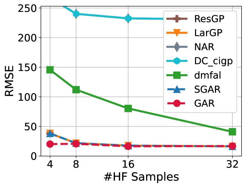
(a) Poisson’s

(b) Burger’s

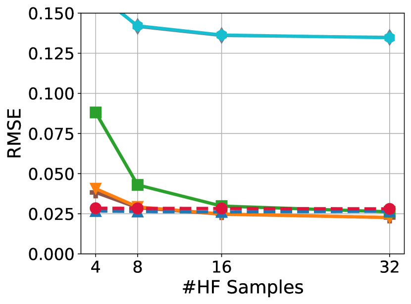
(c) Heat’s

Figure 6: RMSE against increasing number of high-fidelity training samples with training samples increased using Sobol sequence and aligned (interpolated) outputs.

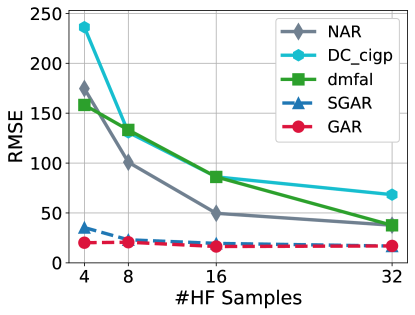
(a) Poisson’s

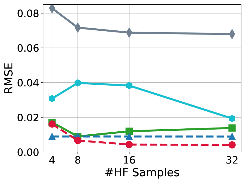
(b) Burger’s

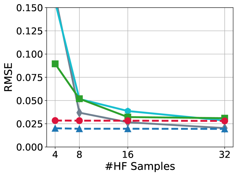
(c) Heat’s

Figure 7: RMSE against increasing number of high-fidelity training samples with training samples increased using Sobol sequence and unaligned outputs.

We use the same experimental setup as in Section 5.1 for these experiments with the only difference being that the training data is generated using a Sobol sequence. We generated 256 data samples for testing and 32 samples for training. We increased the number of high-fidelity training data gradually from 4 to 32 with the high-fidelity training data fixed to 32. Fig. 6 and Fig. 7 show the RMSE statistical results for aligned outputs using interpolated and original unaligned outputs. GAR and CIGAR outperform the competitors with a large margin with scarce high-fidelity training data as in the main paper. Similarly, the advantage of GAR and CIGAR are more obvious when dealing with non-aligned outputs, where GAR and CIGAR demonstrate a 5x reduction in RMSE with 4 and 8 high-fidelity training samples, surpassing the competitors by a wide margin.

E.3 Multi-Fidelity Fusion for Topology Optimization

We use GAR in a topology structure optimization problem, where the output is the best topology structure (in terms of maximum mechanical metrics like stiffness) of a layout of materials, such as alloy and concrete, given some design parameters like external force and angle. Topology structure optimization is a significant approach in mechanical designs, such as airfoils and slab bridges, especially with recent 3D printing processes in which material is deposited in minute quantities. However, it is well known that topology optimization is computationally intensive due to the gradient-based optimization and simulations of the mechanical characteristics involved. A high-fidelity solution, which necessitates a huge discretization mesh and imposes a significant computing overhead in space and time, makes matters worse.

Utilizing data-driven ways to aid in the process by offering the appropriate structures [68, 13] is subsequently gaining popularity. Here, we investigate the topology optimization of a cantilever beam (shown in the appendix). We employ the rapid implementation [69] to carry out density-based topology optimization by reducing compliance $C$ subject to volume limitations $V\leq\bar{V}$.

The SIMP scheme [70] is used to convert continuous density measurements to discrete, optimal topologies. We set the position of point load $P1$, the angle of point load $P2$, and the filter radius $P3$ [55] as system input. We solve this challenge for low-fidelity with a $40\times 80$ regular mesh and high-fidelity with a $40\times 80$ regular mesh. This experiment only includes techniques that can process arbitrary outputs.

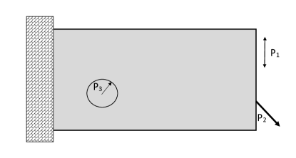
Figure 8: Geometry, boundary conditions, and simulation parameters for cantilever beam

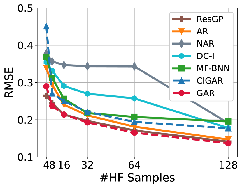
(a) Aligned outputs

(b) Raw outputs

Figure 9: RMSE against increasing number of high-fidelity training samples for topology optimization using Sobol sequence.

As with the early experiments, we generate 128 testing samples and 64 training samples using a Sobol sequence to approximately assess the ance in active learning. The results are shown in Figure 9. We can see that all available methods show similar performance for both raw outputs that are not aligned by interpolation and the aligned outputs. Nevertheless, GAR consistently outperforms the competitors with a clear margin. CIGAR, in contrast, performs better for the raw outputs.

E.4 Multi-Fidelity Fusion for Solid Oxide Fuel Cell

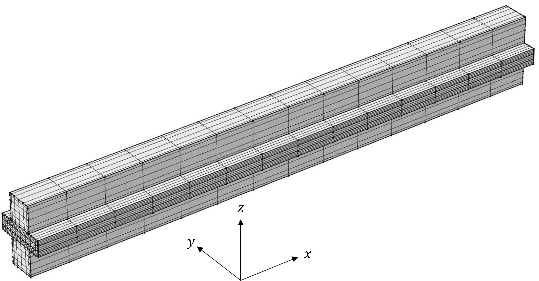
Figure 10: The cathode is at the top of the computational domain for the SOFC example, which consists of gas channels, electrodes, and electrolyte. The layers are, from top to bottom, a channel, an electrode, an electrolyte, an electrode, and a channel. The dimensions of the channel are (x * y * z) 1 cm * 0.5 mm * 0.5 mm, the dimensions of the electrode are 1 cm * 1 mm * 0.1 mm, and the dimensions of the electrolyte are 1 cm * 1 mm * 0.1 mm. The cathode intake is placed at $x=1$ cm while the anode inlet is located at $x=0$ cm.

In this test problem, a steady-state 3-D solid oxide fuel cell model is considered. Fig.10 illustrates the geometry. The model incorporates electronic and ionic charge balances (Ohm’s law), flow distribution in gas channels (Navier-Stokes equations), flow in porous electrodes (Brinkman equation), and gas-phase mass balances in both gas channels and porous electrodes (Maxwell-Stefan diffusion and convection). Butler-Volmer charge transfer kinetics is assumed for reactions in the anode ($\mbox{H}_{2}+\mbox{O}^{2-}\rightarrow\mbox{H}_{2}\mbox{O}+2\mbox{e}^{-}$) and cathode ($\mbox{O}_{2}+4\mbox{e}^{-}\rightarrow 2\mbox{O}^{2-}$). The cell functions in a potentiostat manner (constant cell voltage). COMSOL Multiphysics (Application ID: 514), which uses the finite-element approach, was used to solve the model.

The assumed inputs are the electrode porosities $\epsilon\in[0.4,0.85]$, the cell voltage $E_{c}\in[0.2,0.85]$ V, the temperature $T\in[973,1273]$ K, and the channel pressure $P\in[0.5,2.5]$ atm. A Sobol sequence is used to choose 60 inputs within the ranges specified for the low-fidelity and high-fidelity simulations. 40 high-fidelity test points are chosen at random (from the ranges above) to complete the test. The low-fidelity F1 model used 3164 mapped elements and relative tolerance of 0.1, while the high-fidelity model employed 37064 elements and relative tolerance of 0.001. Additionally, the COMSOL model employs a V cycle geometric multigrid. The quantities of interest are profiles of electrolyte current density (A m$-2$) and ionic potential (V) in the $x-z$ plane centered on the channels (Fig. 10). In both instances, $d=100\times 50=5000$ points are captured, and both profiles are vectorized to provide the training and test outputs.

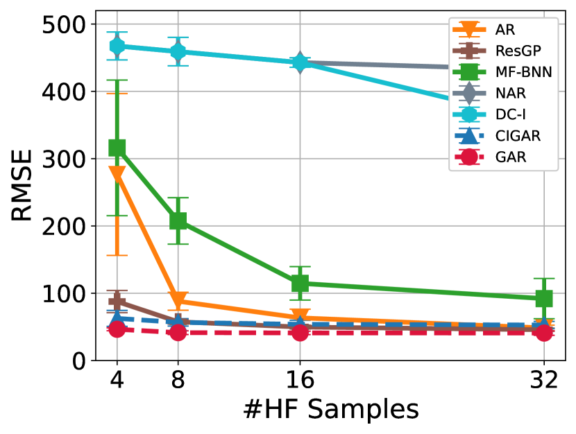
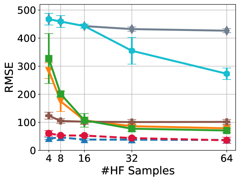
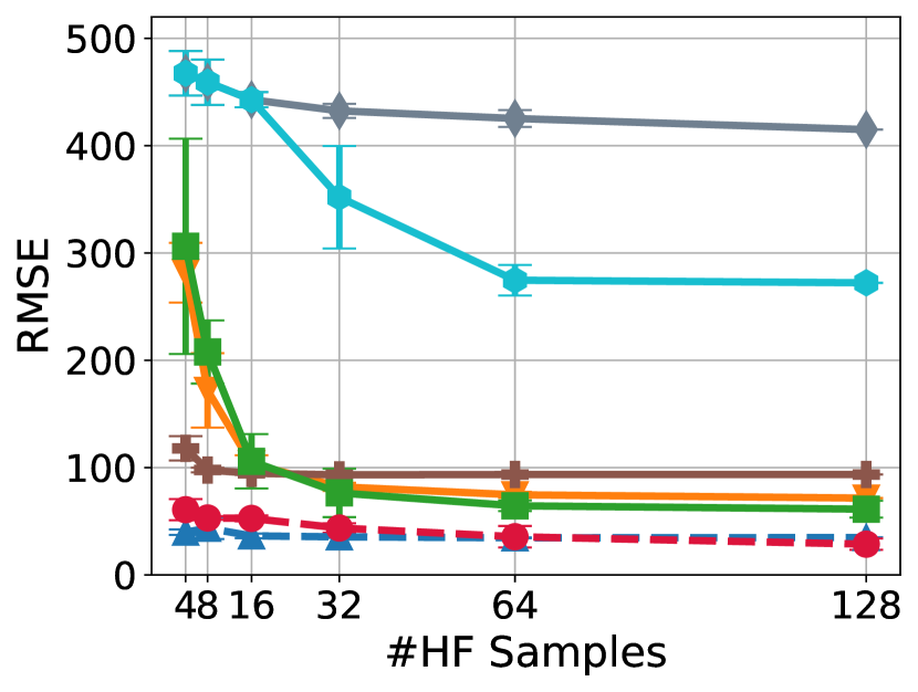
Figure 11: RMSE against increasing number of high-fidelity training samples for SOFC with low-fidelity training sample number fixed to {32,64,128}.

We add the classic experiment where the number of low-fidelity training samples was fixed to {32,64,128} and the high-fidelity training samples are gradually increased from 4 to {32,64,128}. The outputs are aligned using interpolation, and the experimental results are shown in Fig. 11. We can see that the GAR and CIGAR methods always perform better than the other methods, especially when only a few high-fidelity training data are used. This is consistent with the previous experiment. We can also see that AR also performs well indicating that these data are not highly nonlinear and complex, making it relatively easy to solve. However, both AR and MF-BNN converge to a higher error whereas GAR and CIGAR converge to a lower error bound.

(a) NAR

(b) MF-BNN

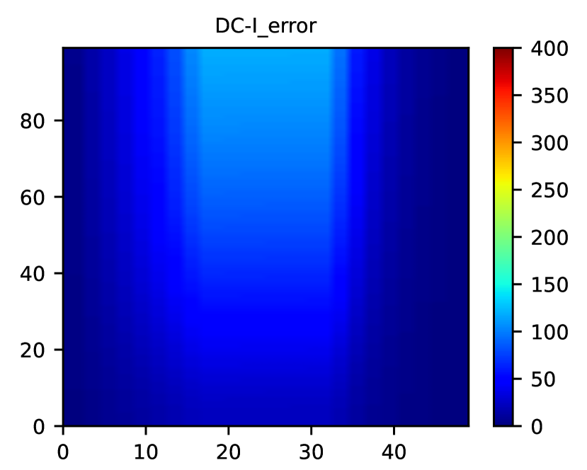
(c) DC

Figure 12: RMSE fields of ECD for 128 testing samples, using 32 low-fidelity and 16 high-fidelity training samples.

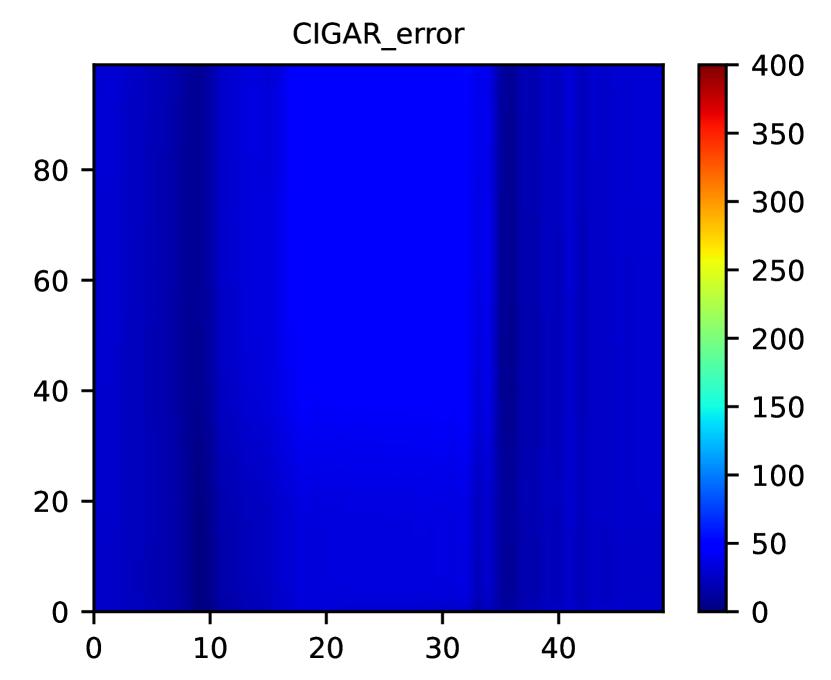
(a) CIGAR

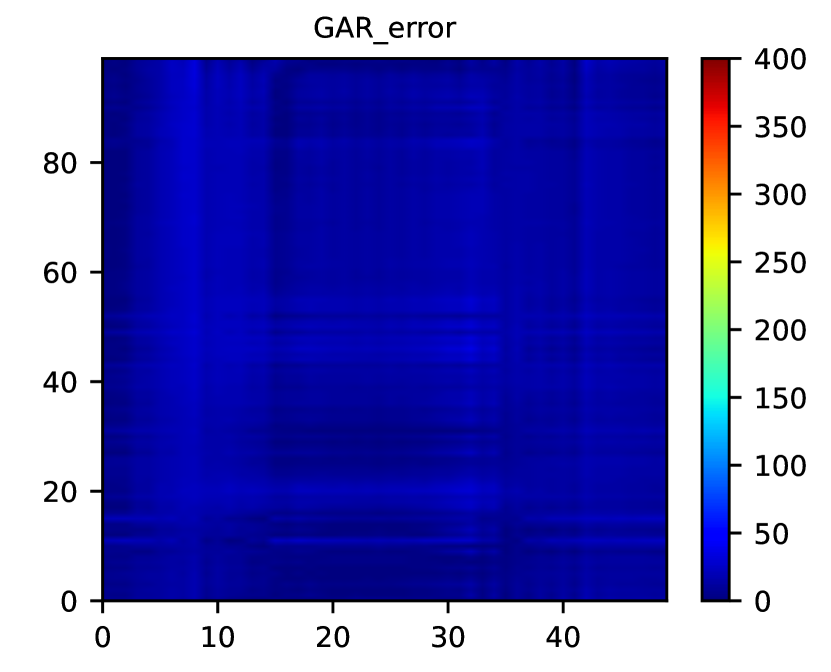
(b) GAR

Figure 13: RMSE fields of ECD for 128 testing samples, using 32 low-fidelity and 4 high-fidelity training samples.

To investigate the prediction error in detail, we define the average RMSE field ${\bm{\mathsfit{Z}}}^{(\mathrm{AEF})}$ by

$${\bm{\mathsfit{Z}}}^{(\mathrm{AEF})}=\sqrt{\frac{1}{N}\sum_{i=1}^{N}({\bm{\mathsfit{Z}}}_{i}-\tilde{{\bm{\mathsfit{Z}}}}_{i})^{2}},$$

where $\tilde{{\bm{\mathsfit{Z}}}}_{i}$ is the prediction, ${\bm{\mathsfit{Z}}}_{i}$ is the ground true value, and the square root is element-wise operation. Fig. 12 shows the average RMSE field of NAR, MF-BNN, and DC methods on the ECD in SOFC data with 32 low-fidelity training samples, 16 high-fidelity training samples, and 128 test samples. To highlight the advantage of GAR and CIGAR, Fig. 13 shows the average RMSE field of the same setup with only 4 high-fidelity training samples. It can be seen clearly that GAR and CIGAR have a smaller error field even with only 4 high-fidelity training samples compared to NAR, MF-BNN, and DC with 16 high-fidelity training samples. Also note that GAR seems to have some checkerboard artifacts, which might be caused by the over-parameterization using a full transfer matrix. We leave this issue to our further work to resolve. CIGAR have fewer checkerboard artifacts with the price of a slight increase in the RMSE.

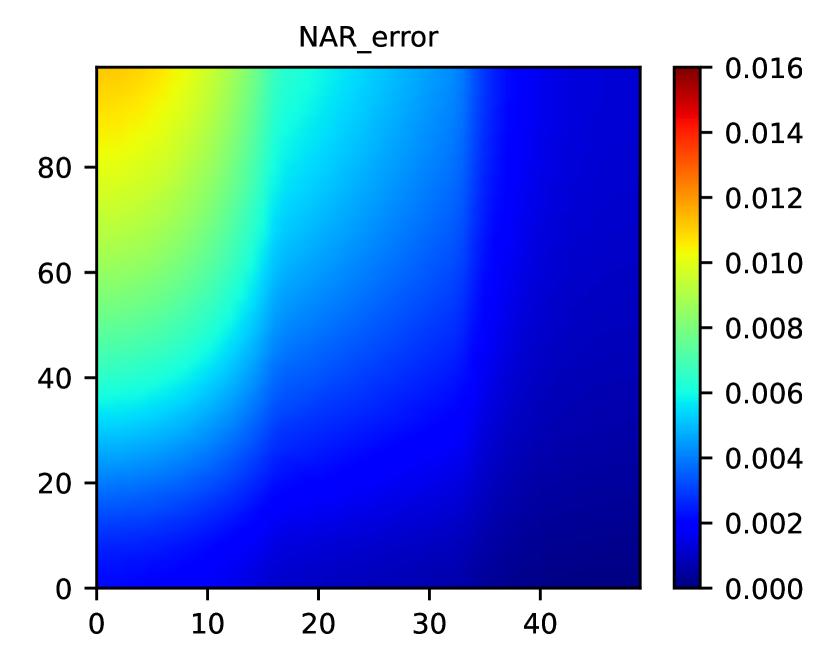
(a) NAR

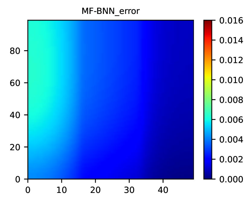
(b) MF-BNN

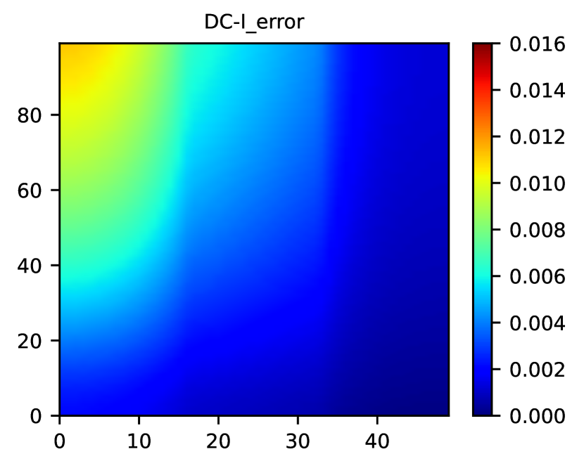
(c) DC

Figure 14: RMSE fields of IP for 128 testing samples, using 32 low-fidelity and 16 high-fidelity training samples.

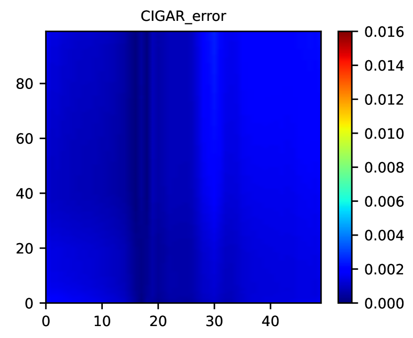
(a) CIGAR

(b) GAR

Figure 15: RMSE fields of IP for 128 testing samples, using 32 low-fidelity and 4 high-fidelity training samples.

In Fig. 14 and Fig. 15, similar to the previous experimental setup, we draw the average RMSE with 128 testing samples on the IP fields from the SOFC dataset. The NAR, MF-BNN and DC are trained with 16 high-fidelity samples, while GAR and CIGAR are trained with only 4 high-fidelity samples. We can see that our methods outperform other methods by a clear margin. However, the checkerboard artifact is even worse for GAR in this case, whereas CIGAR successfully reduces such an artifact with also low error.

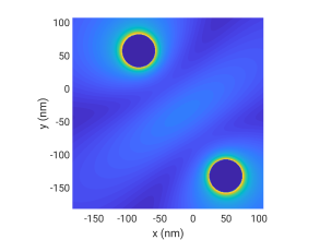
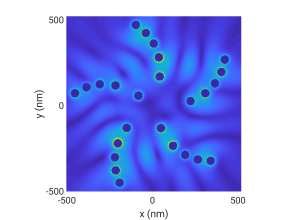
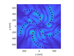
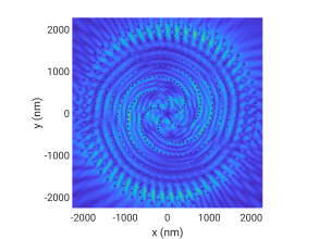
Figure 16: Sample configurations of Vogel spirals with $\{2,25,50,500\}$ particles.

E.5 Plasmonic Nanoparticle Arrays Simulations

In the final example, we calculate the extinction and scattering efficiencies $Q_{ext}$ and $Q_{sc}$ for plasmonic systems with varying numbers of scatterers using the Coupled Dipole Approximation (CDA) approach. CDA is a method for mimicking the optical response of an array of similar, non-magnetic metallic nanoparticles with dimensions far smaller than the wavelength of light (here 25 nm). $Q_{ext}$ and $Q_{sc}$ are defined as the QoIs in this document. We construct surrogate models for efficiency with up to three fidelities using our proposed method. We examine particle arrays resulting from Vogel spirals. Since the number of interactions of incident waves from particles influences the magnetic field, the number of nanoparticles in a plasmonic array has a substantial effect on the local extinction field caused by plasmonic arrays. The configurations of Vogel spirals with particle numbers in the set $\{2,25,50\}$ that define fidelities F1 through F3 are depicted in Fig. 16. $\lambda\in[200,800]$ nm, $\alpha_{vs}\in[0,2\pi]$ rad, and $a_{vs}\in(1,1500)$ are determined to be the parameter space. These are, respectively, the incidence wavelength, the divergence angle, and the scaling factor. A Sobol sequence is utilized to choose inputs. The computing time requires to execute CDA increases exponentially as the number of nanoparticles increases. Consequently, the proposed sampling approach results in significant reductions in computational costs.

The response of a plasmonic array to electromagnetic radiation is calculable using the solution of the local electric fields, ${\bf E}_{loc}({\bf r}_{j})$, for each nano-sphere. Considering $N$ metallic particles defined by the same volumetric polarizability $\alpha(\omega)$ and situated at vector coordinates ${\bf r}_{i}$, it is possible to calculate the local field ${\bf E}_{loc}({\bf r}_{j})$ by solving [71] the corresponding linear equation.

$${\bf E}_{loc}(\mathbf{r}_{i})=\mathbf{E}_{0}({\mathbf{r}_{i}})-\frac{\alpha k^{2}}{\epsilon_{0}}\sum_{j=1,j\neq i}^{N}\mathbf{\tilde{G}}_{ij}\mathbf{E}_{loc}(\mathbf{r}_{j})$$ (A.62)

in which $\mathbf{E}_{0}({\bf r}_{i})$ is the incident field, $k$ is the wave number in the background medium, $\epsilon_{0}$ denotes the dielectric permittivity of vacuum ($\epsilon_{0}=1$ in the CGS unit system), and $\mathbf{\tilde{G}}_{ij}$ is constructed from $3\times 3$ blocks of the overall $3N\times 3N$ Green’s matrices for the $i$th and $j$th particles. $\mathbf{\tilde{G}}_{ij}$ is a zero matrix when $j=i$, and otherwise calculated as

$$\tilde{\bf G}_{ij}=\frac{\exp(ikr_{ij})}{r_{ij}}\left\{{\bf I}-\widehat{{\bf r}}_{ij}\widehat{{\bf r}}_{ij}^{T}-\left[\frac{1}{ikr_{ij}}+\frac{1}{(kr_{ij})^{2}}({\bf I}-3\widehat{{\bf r}}_{ij}\widehat{{\bf r}}_{ij}^{T})\right]\right\}$$ (A.63)

where $\widehat{{\bf r}}_{ij}$ denotes the unit position vector from particles $j$ to $i$ and $r_{ij}=|{\bf r}_{ij}|$. By solving Eqs. A.62 and A.63, the total local fields $\mathbf{E}_{loc}({\bf r}_{i})$, and as a result the scattering and extinction cross-sections, are computed. Details of the numerical solution can be found in [72].

$Q_{ext}$ and $Q_{sc}$ are derived by normalizing the scattering and extinction cross-sections relative to the array’s entire projected area. We considered the Vogel spiral class of particle arrays, which is described by [73]

$$\rho_{n}=\sqrt{n}a_{vs}\quad\mbox{and}\quad\theta_{n}=n\alpha_{vs},$$ (A.64)

where $\rho_{n}$ and $\theta_{n}$ represent the radial distance and polar angle of the $n$-th particle in a Vogel spiral array, respectively. Therefore, the Vogel spiral configuration may be uniquely defined by the incidence wavelength $\lambda$, the divergence angle $\alpha_{vs}$, the scaling factor $a_{vs}$, and the number of particles $n$.

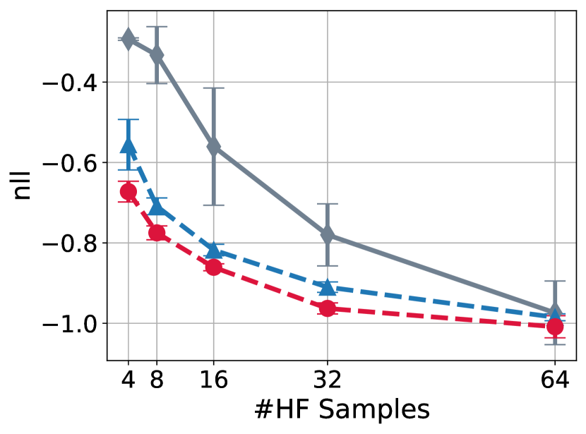
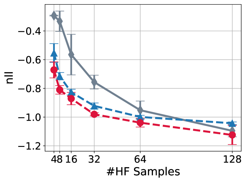
Figure 17: NLL with low-fidelity training sample number fixed to {32,64,128} for topology structure predictions.

(a) ECD+IP

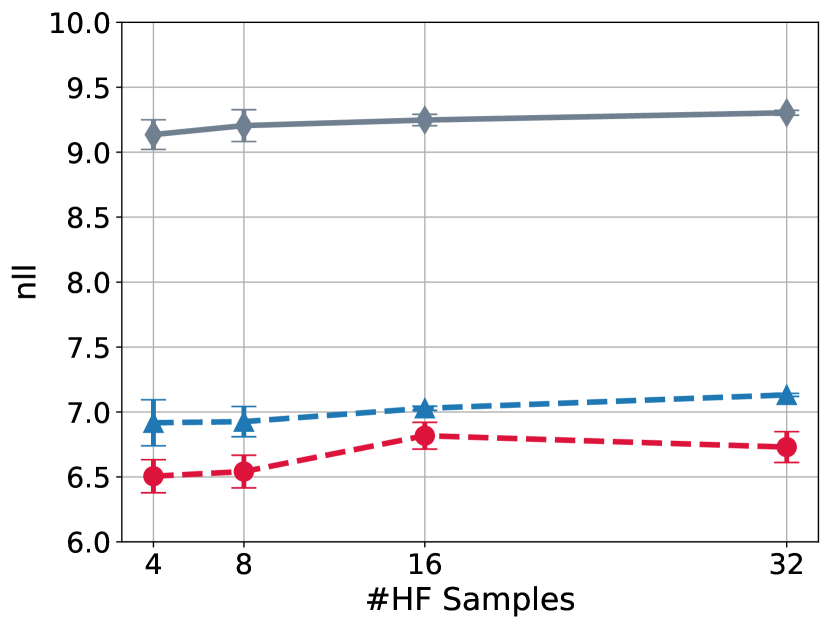
(b) ECD

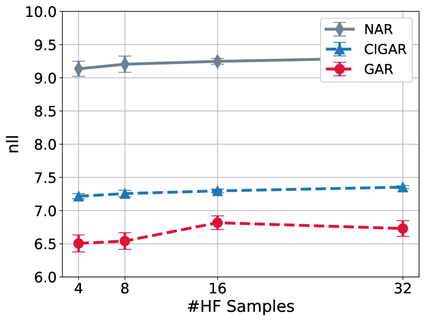
(c) IP

Figure 18: NLL for SOFC with low-fidelity training sample number fixed to 32.

E.6 Metircs for the Predictive Uncertainty

Despite that RMSE has been used as a standard metric for evaluating the performance of a multi-fidelity fusion algorithm [9, 12, 13, 16], a metric that considers the predictive uncertainty is also important [47], particularly when the downstream applications rely heavily on the quality of the predictive confidence, e.g., in MFBO [23]. To assess the proposed method more comprehensively, we evaluate the quality of the predictive posterior using the most commonly used metric, negative-log-likelihood (nll).

We repreduce Figs. 2 and 5 using exactly the same experimental setups but with the nll metric, and the results are shown in Figs. 17 and 18. Note that the nll of DC and MF-BNN is every poor, probably due to our implementations, and cannot be fitted into the figures. Thus they are not shown in the figures. Also note that some figures show negative nll. This is because our computation of the nll omits the constant term. Nevertheless, this modification does not affect the comparison. We can see that for the topology structure posterior in Fig. 17, the results are consistent with the conclusion drawn on the RMSE results. Since the CIGAR ignores the inter-output correlations, it will overestimate the covariance determinant, leading to higher nll than GAR. The NAR starts with poor performance with a small number of training data. It consistently improves with increasing number of training data and end up with similar perform as GAR and CIGAR. Similarly, the SOFC results are consistent with the conclusion for the RMSE results. However, all methods demonstrated do not improve their performance significantly with more training data. This is caused by the calculations of the nll and the data itself. More specifically, in the ECD and IP fields, there are a few spatial locations where the recorded values are almost constant (caused by the Dirichlet boundary conditions). In this case, the nll will be dominated by the logarithm of variance and becomes less informative for the quality of the predictive variance. We thus see that the nll in Fig. 18 fluctuates around the same values no matter how many training points are used. We leave investigating the uncertainty metric using more advance metric (e.g., [74]) more in depth in the future considering the scope of this work.

References

• [1] Bobak Shahriari, Kevin Swersky, Ziyu Wang, Ryan P. Adams, and Nando Freitas. Taking the Human Out of the Loop: A Review of Bayesian Optimization. 104(1):148–175. ISSN 0018-9219, 1558-2256. doi: 10.1109/JPROC.2015.2494218. URL https://ieeexplore.ieee.org/document/7352306/.
• [2] Apostolos F. Psaros, Xuhui Meng, Zongren Zou, Ling Guo, and George Em Karniadakis. Uncertainty Quantification in Scientific Machine Learning: Methods, Metrics, and Comparisons.
• [3] M. Kennedy. Predicting the output from a complex computer code when fast approximations are available. 87(1):1–13. ISSN 0006-3444, 1464-3510. doi: 10.1093/biomet/87.1.1.
• Poloczek et al. [2017] Matthias Poloczek, Jialei Wang, and Peter Frazier. Multi-information source optimization. Advances in neural information processing systems, 30, 2017.
• [5] Jialin Song, Yuxin Chen, and Yisong Yue. A General Framework for Multi-fidelity Bayesian Optimization with Gaussian Processes. In The 22nd International Conference on Artificial Intelligence and Statistics, pages 3158–3167. URL http://proceedings.mlr.press/v89/song19b.html.
• [6] L. Parussini, D. Venturi, P. Perdikaris, and G.E. Karniadakis. Multi-fidelity Gaussian process regression for prediction of random fields. 336(C):36–50. ISSN 0021-9991. doi: 10.1016/j.jcp.2017.01.047.
• Xing et al. [a] W. Xing, M. Razi, R. M. Kirby, K. Sun, and A. A. Shah. Greedy nonlinear autoregression for multifidelity computer models at different scales. 1:100012, a. ISSN 2666-5468. doi: 10.1016/j.egyai.2020.100012. URL https://www.sciencedirect.com/science/article/pii/S2666546820300124.
• [8] Zheng Wang, Wei Xing, Robert Kirby, and Shandian Zhe. Multi-Fidelity High-Order Gaussian Processes for Physical Simulation. In International Conference on Artificial Intelligence and Statistics, pages 847–855. PMLR. URL http://proceedings.mlr.press/v130/wang21c.html.
• Xing et al. [b] W. W. Xing, A. A. Shah, P. Wang, S. Zhe, Q. Fu, and R. M. Kirby. Residual gaussian process: A tractable nonparametric bayesian emulator for multi-fidelity simulations. 97:36–56, b. ISSN 0307-904X. doi: 10.1016/j.apm.2021.03.041. URL https://www.sciencedirect.com/science/article/pii/S0307904X21001724.
• [10] M. Giselle Fernández-Godino, Chanyoung Park, Nam-Ho Kim, and Raphael T. Haftka. Review of multi-fidelity models.
• [11] B. Peherstorfer, K. Willcox, and M. Gunzburger. Survey of Multifidelity Methods in Uncertainty Propagation, Inference, and Optimization. 60(3):550–591. ISSN 0036-1445. doi: 10.1137/16M1082469.
• Xing et al. [c] Wei W. Xing, Robert M. Kirby, and Shandian Zhe. Deep coregionalization for the emulation of simulation-based spatial-temporal fields. 428:109984, c. ISSN 0021-9991. doi: 10.1016/j.jcp.2020.109984. URL https://linkinghub.elsevier.com/retrieve/pii/S0021999120307580.
• Li et al. [2020] Shibo Li, Robert M Kirby, and Shandian Zhe. Deep multi-fidelity active learning of high-dimensional outputs. arXiv preprint arXiv:2012.00901, 2020.
• [14] Mauricio A. Alvarez, Lorenzo Rosasco, and Neil D. Lawrence. Kernels for Vector-Valued Functions: A Review.
• [15] Loic Le Gratiet. Bayesian Analysis of Hierarchical Multifidelity Codes. 1(1):244–269. ISSN 2166-2525. doi: 10.1137/120884122.
• [16] Paris Perdikaris, M Raissi, Andreas Damianou, N D. Lawrence, and George Karniadakis. Nonlinear Information Fusion Algorithms for Data-Efficient Multi-Fidelity Modelling, volume 473. Royal Society. doi: 10.1098/rspa.2016.0751.
• [17] Carl Edward Rasmussen and Christopher K I Williams. Gaussian Processes for Machine Learning. page 266.
• [18] Shandian Zhe, Wei Xing, and Robert M. Kirby. Scalable High-Order Gaussian Process Regression. In The 22nd International Conference on Artificial Intelligence and Statistics, pages 2611–2620. PMLR. URL http://proceedings.mlr.press/v89/zhe19a.html.
• [19] Tamara Gibson Kolda. Multilinear operators for higher-order decompositions. URL http://www.osti.gov/servlets/purl/923081-u0xXJa/.
• [20] Zenglin Xu, Feng Yan, Yuan, and Qi. Infinite Tucker Decomposition: Nonparametric Bayesian Models for Multiway Data Analysis.
• [21] Andrew Gordon Wilson and Hannes Nickisch. Kernel interpolation for scalable structured Gaussian processes (KISS-GP). In Proceedings of the 32nd International Conference on International Conference on Machine Learning - Volume 37, ICML’15, pages 1775–1784. JMLR.org.
• Perrone et al. [2018] Valerio Perrone, Rodolphe Jenatton, Matthias W Seeger, and Cédric Archambeau. Scalable hyperparameter transfer learning. Advances in neural information processing systems, 31, 2018.
• Li et al. [a] Shibo Li, Wei Xing, Robert Kirby, and Shandian Zhe. Multi-Fidelity Bayesian Optimization via Deep Neural Networks. 33:8521–8531, a. URL https://papers.nips.cc/paper/2020/hash/60e1deb043af37db5ea4ce9ae8d2c9ea-Abstract.html.
• [24] Akil Narayan, Claude Gittelson, and Dongbin Xiu. A Stochastic Collocation Algorithm with Multifidelity Models. 36(2):A495–A521. ISSN 1064-8275. doi: 10.1137/130929461.
• [25] Kurt Cutajar, Mark Pullin, Andreas Damianou, Neil Lawrence, and Javier González. Deep Gaussian Processes for Multi-fidelity Modeling.
• Wilson and Adams [2013] Andrew Wilson and Ryan Adams. Gaussian process kernels for pattern discovery and extrapolation. In International conference on machine learning, pages 1067–1075. PMLR, 2013.
• [27] Mauricio A. Álvarez, Lorenzo Rosasco, and Neil D. Lawrence. Kernels for Vector-Valued Functions: A Review. 4(3):195–266. ISSN 1935-8237, 1935-8245. doi: 10.1561/2200000036. URL http://www.nowpublishers.com/article/Details/MAL-036.
• Goulard and Voltz [1992] Michel Goulard and Marc Voltz. Linear coregionalization model: tools for estimation and choice of cross-variogram matrix. Mathematical Geology, 24(3):269–286, 1992.
• Goovaerts et al. [1997] Pierre Goovaerts et al. Geostatistics for natural resources evaluation. Oxford University Press on Demand, 1997.
• Teh et al. [2005] Yee Whye Teh, Matthias Seeger, and Michael I Jordan. Semiparametric latent factor models. In International Workshop on Artificial Intelligence and Statistics, pages 333–340. PMLR, 2005.
• [31] Dave Higdon, James Gattiker, Brian Williams, and Maria Rightley. Computer Model Calibration Using High-Dimensional Output. 103(482):570–583. ISSN 0162-1459, 1537-274X. doi: 10.1198/016214507000000888.
• Xing et al. [d] W.W. Xing, V. Triantafyllidis, A.A. Shah, P.B. Nair, and N. Zabaras. Manifold learning for the emulation of spatial fields from computational models. 326:666–690, d. ISSN 0021-9991. doi: 10.1016/j.jcp.2016.07.040. URL https://linkinghub.elsevier.com/retrieve/pii/S0021999116303722.
• Xing et al. [e] Wei Xing, Akeel A. Shah, and Prasanth B. Nair. Reduced dimensional Gaussian process emulators of parametrized partial differential equations based on Isomap. 471(2174):20140697, e. ISSN 1364-5021, 1471-2946. doi: 10.1098/rspa.2014.0697.
• Álvarez et al. [2019] Mauricio A Álvarez, Wil Ward, and Cristian Guarnizo. Non-linear process convolutions for multi-output gaussian processes. In The 22nd International Conference on Artificial Intelligence and Statistics, pages 1969–1977. PMLR, 2019.
• Boyle and Frean [2004] Phillip Boyle and Marcus Frean. Dependent gaussian processes. Advances in neural information processing systems, 17, 2004.
• [36] Dave Higdon. Space and Space-Time Modeling using Process Convolutions. In Clive W. Anderson, Vic Barnett, Philip C. Chatwin, and Abdel H. El-Shaarawi, editors, Quantitative Methods for Current Environmental Issues, pages 37–56. Springer London. ISBN 978-1-4471-1171-9 978-1-4471-0657-9. doi: 10.1007/978-1-4471-0657-9_2.
• Bonilla et al. [2007] Edwin V Bonilla, Felix V Agakov, and Christopher KI Williams. Kernel multi-task learning using task-specific features. In Artificial Intelligence and Statistics, pages 43–50. PMLR, 2007.
• Rakitsch et al. [2013] Barbara Rakitsch, Christoph Lippert, Karsten Borgwardt, and Oliver Stegle. It is all in the noise: Efficient multi-task gaussian process inference with structured residuals. Advances in neural information processing systems, 26, 2013.
• [39] Ping Li and Songcan Chen. Hierarchical Gaussian Processes model for multi-task learning. 74:134–144. ISSN 0031-3203. doi: 10.1016/j.patcog.2017.09.021. URL https://linkinghub.elsevier.com/retrieve/pii/S0031320317303746.
• Wilson et al. [2012] Andrew Gordon Wilson, David A. Knowles, and Zoubin Ghahramani. Gaussian process regression networks. In Proceedings of the 29th International Coference on International Conference on Machine Learning, ICML’12, page 1139–1146, Madison, WI, USA, 2012. Omnipress. ISBN 9781450312851.
• Nguyen and Bonilla [2013] Trung Nguyen and Edwin Bonilla. Efficient variational inference for gaussian process regression networks. In Artificial Intelligence and Statistics, pages 472–480. PMLR, 2013.
• [42] Tamara G. Kolda and Brett W. Bader. Tensor Decompositions and Applications. 51(3):455–500. ISSN 0036-1445, 1095-7200. doi: 10.1137/07070111X.
• Li et al. [b] Shibo Li, Wei Xing, Robert M. Kirby, and Shandian Zhe. Scalable Gaussian Process Regression Networks. volume 3, pages 2456–2462, b. doi: 10.24963/ijcai.2020/340. URL https://www.ijcai.org/proceedings/2020/340.
• [44] Andreas Damianou. Deep Gaussian processes and variational propagation of uncertainty.
• Kandasamy et al. [2016] Kirthevasan Kandasamy, Gautam Dasarathy, Junier B Oliva, Jeff Schneider, and Barnabás Póczos. Gaussian process bandit optimisation with multi-fidelity evaluations. Advances in neural information processing systems, 29, 2016.
• Zhang et al. [2017] Yehong Zhang, Trong Nghia Hoang, Bryan Kian Hsiang Low, and Mohan Kankanhalli. Information-based multi-fidelity bayesian optimization. In NIPS Workshop on Bayesian Optimization, 2017.
• Wu et al. [2022] Dongxia Wu, Matteo Chinazzi, Alessandro Vespignani, Yi-An Ma, and Rose Yu. Multi-fidelity hierarchical neural processes. arXiv preprint arXiv:2206.04872, 2022.
• [48] Xuhui Meng and George Em Karniadakis. A composite neural network that learns from multi-fidelity data: Application to function approximation and inverse PDE problems. 401:109020. ISSN 0021-9991. doi: 10.1016/j.jcp.2019.109020. URL http://www.sciencedirect.com/science/article/pii/S0021999119307260.
• Requeima et al. [2019] James Requeima, William Tebbutt, Wessel Bruinsma, and Richard E Turner. The gaussian process autoregressive regression model (gpar). In The 22nd International Conference on Artificial Intelligence and Statistics, pages 1860–1869. PMLR, 2019.
• Xia et al. [2020] Rui Xia, Wessel Bruinsma, William Tebbutt, and Richard E Turner. The gaussian process latent autoregressive model. In Third Symposium on Advances in Approximate Bayesian Inference, 2020.
• [51] Rui Tuo, C. F. Jeff Wu, and Dan Yu. Surrogate Modeling of Computer Experiments With Different Mesh Densities. 56(3):372–380. ISSN 0040-1706, 1537-2723. doi: 10.1080/00401706.2013.842935.
• [52] Mehmet Onder Efe and Hitay Ozbay. Proper orthogonal decomposition for reduced order modeling: 2d heat flow. In Proceedings of 2003 IEEE Conference on Control Applications, 2003. CCA 2003., volume 2, pages 1273–1277. IEEE.
• [53] Maziar Raissi and George Em Karniadakis. Machine Learning of Linear Differential Equations using Gaussian Processes. 348:683–693. ISSN 0021-9991. doi: 10/gbzfgr.
• [54] I.M Sobol’. On the distribution of points in a cube and the approximate evaluation of integrals. 7(4):86–112. ISSN 0041-5553. doi: 10.1016/0041-5553(67)90144-9. URL https://linkinghub.elsevier.com/retrieve/pii/0041555367901449.
• Bruns and Tortorelli [2001] Tyler E. Bruns and Daniel A. Tortorelli. Topology optimization of non-linear elastic structures and compliant mechanisms. Computer Methods in Applied Mechanics and Engineering, 190(26):3443 – 3459, 2001. ISSN 0045-7825. doi: https://doi.org/10.1016/S0045-7825(00)00278-4. URL http://www.sciencedirect.com/science/article/pii/S0045782500002784.
• [56] TJ Chung. Computational fluid dynamics. Cambridge university press.
• [57] N Sugimoto. Burgers equation with a fractional derivative; hereditary effects on nonlinear acoustic waves. 225:631–653.
• [58] Kai Nagel. Particle hopping models and traffic flow theory. 53(5):4655.
• [59] S Kutluay, AR Bahadir, and A Özdecs. Numerical solution of one-dimensional burgers equation: explicit and exact-explicit finite difference methods. 103(2):251–261.
• [60] A. A. Shah, W. W. Xing, and V. Triantafyllidis. Reduced-order modelling of parameter-dependent, linear and nonlinear dynamic partial differential equation models. 473(2200):20160809. ISSN 1364-5021, 1471-2946. doi: 10.1098/rspa.2016.0809.
• [61] Maziar Raissi, Paris Perdikaris, and George Em Karniadakis. Physics informed deep learning (part i): Data-driven solutions of nonlinear partial differential equations.
• [62] Steven C Chapra, Raymond P Canale, et al. Numerical methods for engineers. Boston: McGraw-Hill Higher Education,.
• [63] S Persides. The laplace and poisson equations in schwarzschild’s space-time. 43(3):571–578.
• Lagaris et al. [Sept./1998] I. E. Lagaris, A. Likas, and D. I. Fotiadis. Artificial Neural Networks for Solving Ordinary and Partial Differential Equations. 9(5):987–1000, Sept./1998. ISSN 1045-9227. doi: 10.1109/72.712178.
• [65] Frank Spitzer. Electrostatic capacity, heat flow, and brownian motion. 3(2):110–121.
• [66] Krzysztof Burdzy, Zhen-Qing Chen, John Sylvester, et al. The heat equation and reflected brownian motion in time-dependent domains. 32(1B):775–804.
• [67] Fischer Black and Myron Scholes. The pricing of options and corporate liabilities. 81(3):637–654.
• Xing et al. [f] Wei Xing, Shireen Y. Elhabian, Vahid Keshavarzzadeh, and Robert M. Kirby. Shared-Gaussian Process: Learning Interpretable Shared Hidden Structure Across Data Spaces for Design Space Analysis and Exploration. 142(8), f. ISSN 1050-0472, 1528-9001. doi: 10.1115/1.4046074.
• Andreassen et al. [2011] Erik Andreassen, Anders Clausen, Mattias Schevenels, Boyan S. Lazarov, and Ole Sigmund. Efficient topology optimization in matlab using 88 lines of code. Structural and Multidisciplinary Optimization, 43(1):1–16, Jan 2011. ISSN 1615-1488. doi: 10.1007/s00158-010-0594-7. URL https://doi.org/10.1007/s00158-010-0594-7.
• Bendsoe and Sigmund [2004] Martin Philip Bendsoe and Ole Sigmund. Topology optimization: Theory, methods and applications. Springer, 2004.
• Guérin et al. [2006] Charles-Antoine Guérin, Pierre Mallet, and Anne Sentenac. Effective-medium theory for finite-size aggregates. JOSA A, 23(2):349–358, 2006.
• [72] Mani Razi, Ren Wang, Yanyan He, Robert M. Kirby, and Luca Dal Negro. Optimization of Large-Scale Vogel Spiral Arrays of Plasmonic Nanoparticles. 14(1):253–261. ISSN 1557-1955, 1557-1963. doi: 10.1007/s11468-018-0799-y.
• Christofi et al. [2016] Aristi Christofi, Felipe A Pinheiro, and Luca Dal Negro. Probing scattering resonances of vogel’s spirals with the green’s matrix spectral method. Optics letters, 41(9):1933–1936, 2016.
• Wu et al. [2021] Dongxia Wu, Liyao Gao, Xinyue Xiong, Matteo Chinazzi, Alessandro Vespignani, Yi-An Ma, and Rose Yu. Quantifying uncertainty in deep spatiotemporal forecasting. arXiv preprint arXiv:2105.11982, 2021.