A NOEMA molecular line scan of the Hubble Deep Field North:
Improved constraints on the CO luminosity functions and cosmic density of molecular gas

Abstract

We present measurements of the CO luminosity functions (LFs) and the evolution of the cosmic molecular gas density out to $z\sim 6$ based on an 8.5 arcmin² spectral scan survey at 3 mm of the iconic Hubble Deep Field North (HDF-N) observed with the NOrthern Extended Millimeter Array (NOEMA). We use matched filtering to search for line emission from galaxies and determine their redshift probability distributions exploiting the extensive multi-wavelength data for the HDF-N. We identify the 7 highest-fidelity sources as CO emitters at $1<z<6$, including the well-known submillimeter galaxy HDF 850.1 at $z=5.18$. Four high-fidelity 3 mm continuum sources are all found to be radio galaxies at $z\leq 1$, plus HDF 850.1. We constrain the CO LFs in the HDF-N out to $z\sim 6$, including a first measurement of the CO(5–4) LF at $\langle z\rangle=5.0$. The relatively large area and depth of the NOEMA HDF-N survey extends the existing luminosity functions at $1<z<4$ above the knee, yielding a somewhat lower density by 0.15–0.4 dex at the overlap region for the CO(2–1) and CO(3–2) transitions, attributed to cosmic variance. We perform a joint analysis of the CO LFs in the HDF-N and Hubble Ultra Deep Field from ASPECS, finding that they can be well described by a single Schechter function. The evolution of the cosmic molecular gas density from a joint analysis is in good agreement with earlier determinations. This implies that the impact of cosmic field-to-field variance on the measurements is consistent with previous estimates, adding to the challenges for simulations that model galaxies from first principles.

1 Introduction

As star formation takes place inside clouds of cold molecular gas (McKee & Ostriker, 2007), the cosmic density of molecular gas ($\rho_{\rm mol}$) plays a key role in our understanding of what drives the cosmic star formation rate density (Madau & Dickinson, 2014) and the baryon cycle of matter flowing in and out of galaxies (Walter et al., 2020; Péroux & Howk, 2020).

Measurements of the cosmic molecular gas density have matured over the last decade, in particular through so-called spectral scan surveys in the (sub-)millimeter regime of extragalactic deep fields with large interferometers. By scanning for emission from the low-$J$ transitions of carbon monoxide (CO)—one of the key tracers of cold molecular gas in the local universe (Solomon et al., 1992; Bolatto et al., 2013)—a flux-limited census of the molecular gas reservoirs in galaxies can be obtained, provided the physical conditions of the systems under study are known.

The first constraints on the cosmic molecular gas density from individual CO detections were obtained over a 1 arcmin² area in the Hubble Deep Field North (Williams et al., 1996) in the 3 mm band with the Plateau de Bure Interferometer (PdBI, Walter et al., 2014; Decarli et al., 2014). Building on these, the ALMA Spectroscopic Survey of the Hubble Ultra Deep Field (ASPECS)-Pilot program targeted a $\sim 1$ arcmin² area in the Hubble Ultra Deep Field (Beckwith et al., 2006) in both the 3 mm and 1.2 mm bands at greater depth (Walter et al., 2016; Aravena et al., 2016a, b; Bouwens et al., 2016; Decarli et al., 2016a, b; Carilli et al., 2016). These initial efforts led to the first extragalactic ALMA large program, ASPECS, that covered the entire eXtreme Deep Field region of the HUDF (Illingworth et al., 2013) over a 4.6 arcmin² scan at 3 mm (Aravena et al., 2019; Boogaard et al., 2019, 2021b; Decarli et al., 2019; González-López et al., 2019; Popping et al., 2019; Uzgil et al., 2019) and 1.2 mm (Aravena et al., 2020; Boogaard et al., 2020; Bouwens et al., 2020; Decarli et al., 2020; González-López et al., 2020; Inami et al., 2020; Popping et al., 2020; Magnelli et al., 2020). At the same time a significantly larger $\sim 60$ arcmin² area in the COSMOS and GOODS-North fields was targeted as part of the COLDz survey at 9 mm (Pavesi et al., 2018; Riechers et al., 2019) on the Karl G. Jansky Very Large Array, probing the bright end of the luminosity function for lower-$J$ CO transitions at similar or higher redshifts.

Through the larger area and complementary line and redshift coverage, these surveys have provided an increasingly detailed picture of the cosmic molecular gas density out to $z\sim 4$. These reveal that $\rho_{\rm mol}(z)$ increases by a factor $\sim 6\times$ going out to $z\sim 1.5$, with a subsequent decline out to the highest redshifts probed (Walter et al., 2020). However, the speed at which spectral scan surveys can be conducted is limited by the bandwidth that can be observed per tuning ($\sim 4$ GHz per sideband for ALMA) and the requirement to perform mosaicing over larger areas. This implies that the deepest surveys to date are still probing volumes that are subject to cosmic variance (Decarli et al., 2020; Popping et al., 2020), though the three-dimensional volumes probed are significantly larger than the modest on-sky areas may suggest.

To address these issues, we have conducted a new survey using the NOrthern Extended Millimeter Array (NOEMA), covering the full Hubble Deep Field North in a 45 pointing mosaic encompassing 8.5 arcmin² at 3 mm. Capitalising on the quadrupled instantaneous bandwidth of the POLYFIX correlator (compared to the original PdBI scan) of 16 GHz and the increased sensitivity from four extra antennas in the array, we cover almost the full 3 mm window between 82—113 GHz in only 2 setups. For comparison, the NOEMA HDF-N survey covers almost $\sim 2\times$ the area of ASPECS at a $\sim 3\times$ shallower depth.

This paper is organised as follows. In § 2 we present the observations and data reduction. We discuss the line search, the identification of both the line and continuum emitters, and the subsequent computation of the luminosity functions (LF) in § 3, also including a comparison to the original PdBI scan. We discuss constraints on the CO LFs and the cosmic molecular gas density in § 4. We summarize and conclude in § 5. Throughout this paper, we adopt a Planck Collaboration et al. (2020) cosmology (flat $\Lambda$CDM with $H_{0}=67.66$ km s^-1 Mpc^-1, $\Omega_{m}=0.3111$ and $\Omega_{\Lambda}=0.6889$). We use $\log$ to denote $\log_{10}$ and $\ln$ for the natural logarithm.

Table 1: Lines and corresponding redshift ranges and volume covered in the HDF-N mosaic.

Transition	$\nu_{\rm rest}$	$z_{\rm min}$	$z_{\rm max}$	$\langle z\rangle$	Volume
	($\mathrm{GHz}$)				($\mathrm{Mpc^{3}}$)
(1)	(2)	(3)	(4)	(5)	(6)
CO(1–0)	115.271	0.0173	0.399	0.2936	995
CO(2–1)	230.538	1.0345	1.798	1.4389	19963
CO(3–2)	345.796	2.0517	3.1969	2.6276	34591
CO(4–3)	461.041	3.0687	4.5956	3.8210	42446
CO(5–4)	576.268	4.0856	5.9941	5.0156	46693
CO(6–5)	691.473	5.1023	7.3923	6.2106	49016
CO(7–6)	806.652	6.1188	8.7902	7.4056	50251
$\mathrm{[C\,\textsc{i}]}$(1–0)	492.161	3.3434	4.9733	4.1436	43857
$\mathrm{[C\,\textsc{i}]}$(2–1)	809.342	6.1425	8.8228	7.4335	50271

Note. — The frequency coverage ranges from 82.394 – 113.322 GHz. The comoving volume and volume-weighted average redshifts are computed within 0.5 of the primary beam peak sensitivity (8.5 arcmin² at 98 GHz), accounting for its frequency dependence.

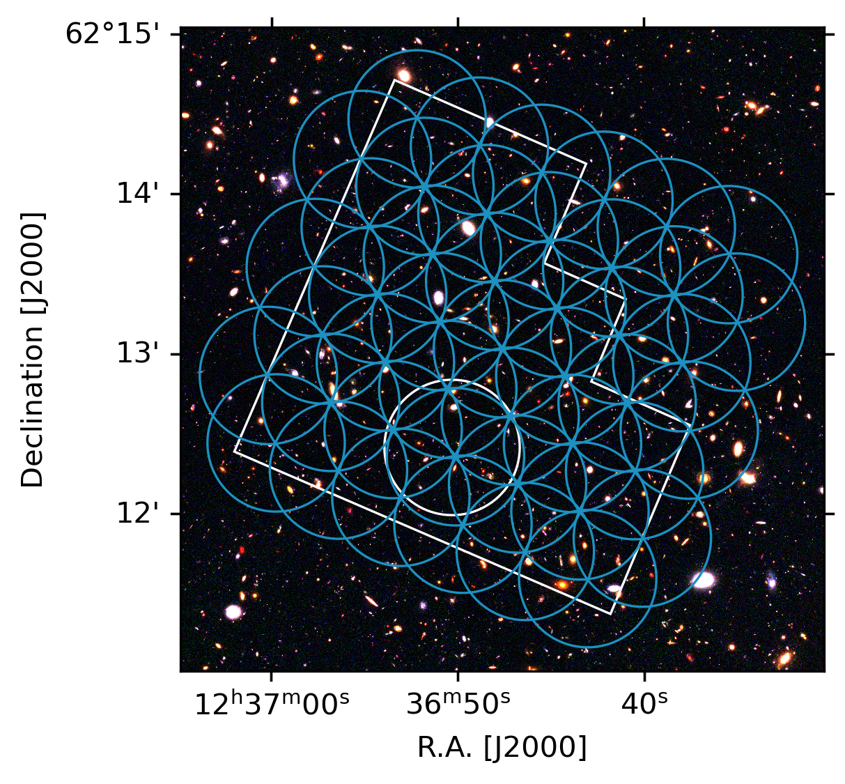
Figure 1: Footprint of the 45-pointing NOEMA mosaic around the central frequency of 98 GHz (in blue) compared to the footprint of the original Hubble Deep Field North observations with WFPC2 from Williams et al. (1996, in white). The white circle indicates the original Plateau de Bure scan (Walter et al., 2014; Decarli et al., 2014). The background shows the Hubble imaging from CANDELS (Grogin et al., 2011; Koekemoer et al., 2011) in the WFC3/F160W, ACS/F850LP, and ACS/F606W filters (RGB).

Table 2: Properties of the dirty cubes and continuum map.

Tuning	$\nu_{0}$	Beam size	Beam P.A.	$\langle\mathrm{rms}\rangle$
	(GHz)	(arcsec2)	(degrees)	(mJy beam-1)
(1)	(2)	(3)	(4)	(5)
Setup 1 LSB	86.300	$4.82\times 4.33$	87.9	0.42
Setup 2 LSB	94.026	$4.44\times 3.92$	90.2	0.60
Setup 1 USB	101.600	$4.11\times 3.68$	86.5	0.53
Setup 2 USB	109.362	$3.75\times 3.33$	91.0	0.95
Continuum	97.822	$4.26\times 3.75$	87.4	0.011

Note. — (1) The four sidebands, plus the continuum. (2) Central frequency. (3) Beam size. (4) Beam position angle. (5) Root-mean-square (rms) noise, which for the cubes is the average rms per 9 MHz channel.

2 NOEMA Observations

The NOEMA mosaic consists of 45 pointings that are laid-out in a Nyquist-sampled hexagonal pattern at around 98 GHz, with the phase center set to 12:36:47.60 +62:13:02.0. It covers 8.5 arcmin² (50% peak sensitivity at 98 GHz) in the GOODS-North area, encompassing the complete Hubble Deep Field North (Fig. 1). The mosaic was observed in two setups that cover nearly the full 3 mm band from 82.394–113.322 GHz. The main emission lines that are covered in spectral scan and their associated redshift range and cosmic volume are listed in Table 1.

The observations were taken between the 27th of March and 20th April 2019 for setup 1 and between 9th of May and 15th of October 2020 for setup 2. The calibration of the mosaic was performed in clic. For setup 1, a total of 7 tracks were used in the final reduction. The calibrators were 3C273 and 3C84 for the bandpass, 1125+569 and J1302+690 for the amplitude and phase (using the average polarisation for the amplitude when detected), and LKHA101 and MWC349 for the absolute flux calibration, except for the track on the 2nd of April 2019, for which 1055+018 and 1125+569 were used as the bandpass and flux calibrators respectively. For setup 2, a total of 10 tracks were used, with bandpass calibrators 3C273, 0851+202, 3C84, and 3C345, amplitude and phase calibrator 1125+569, and flux calibrators MWC349 and 3C84.

We create a dirty cube of the entire mosaic for each of the four sidebands separately, with 9 MHz channels and a $0\farcs 75$ pixel size, using Gildas (version August 22a). The reference frequency is set to the center of each sideband and we take into account frequency dependence of the synthesised beam for every channel by explicitly setting $\texttt{map\_beam\_step}=1$ in uvmap. We subsequently compute the (frequency-dependent) sensitivity map of the mosaic (or ‘primary beam of the mosaic’) as the weighted primary beam response of individual pointings. We use the sensitivity map to create both (flux-calibrated) cubes where the noise is flat (that are used for the line search) and sensitivity-map-corrected cubes (with noise increasing towards the edges of the mosaic). The beam shape and root-mean-square (rms) noise of each of the four cubes is detailed in Table 2.

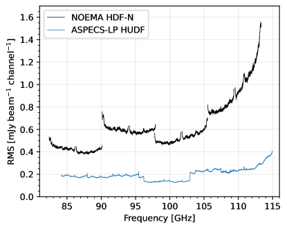
Figure 2: The root-mean-square noise (rms) as a function of frequency. The rms is measured per 9 MHz channel and the upper and lower sidebands of each of the two setups of the NOEMA HDF-N scan are shown separately. For comparison, the rms of the ASPECS-LP (Decarli et al., 2019, measured per 7.8 MHz channel) is shown in blue.

Table 3: Highest fidelity lines from the line search and their identification.

ID	RA	Decl.	S/N	Fidelity	PB	Frequency	FWHM	Integrated flux	$J$	$z$	comment
	(J2000)	(J2000)				($\mathrm{GHz}$)	(km s-1)	(Jy km s-1)
(1)	(2)	(3)	(4)	(5)	(6)	(7)	(8)	(9)	(10)	(11)	(12)
1	12:36:34.52	+62:12:41.0	12.38	1.00	0.48	103.655 $\pm$ 0.008	518 $\pm$ 58	2.14 $\pm$ 0.21	2	1.225	spec-$z$
2	12:36:48.57	+62:12:16.2	7.72	1.00	0.99	82.777 $\pm$ 0.006	325 $\pm$ 53	0.50 $\pm$ 0.07	2	1.785	D14.ID3, spec-$z$
3	12:36:52.00	+62:12:26.0	6.89	1.00	0.99	93.191 $\pm$ 0.011	417 $\pm$ 83	0.58 $\pm$ 0.10	5	5.184	HDF 850.1, spec-$z$
4	12:36:40.73	+62:14:06.5	6.40	0.99	0.69	104.060 $\pm$ 0.014	447 $\pm$ 94	0.76 $\pm$ 0.14	3†	2.323†	$p(z)$ ambiguous
5	12:36:33.01	+62:13:41.0	6.01	0.83	0.52	83.518 $\pm$ 0.016	567 $\pm$ 135	0.88 $\pm$ 0.18	3†	3.141†	$p(z)$ ambiguous
6	12:36:44.81	+62:12:07.2	5.99	0.73	1.00	109.173 $\pm$ 0.003	74 $\pm$ 17	0.29 $\pm$ 0.06	2†	1.112†	$p(z)$ peak ($>90\%$)
7	12:36:38.80	+62:12:57.5	5.85	0.81	0.98	107.494 $\pm$ 0.007	171 $\pm$ 44	0.40 $\pm$ 0.09	2	1.145	spec-$z$

Note. — (1) Line ID. (2–3) Right ascension and declination. (4) S/N from matched filtering. (5) Fidelity. (6) Mosaic sensitivity relative to peak at the source position. (7-9) Line frequency, full-width at half-maximum (FWHM) and integrated flux from a Gaussian fit. (10) Upper $J$ level of identified CO transition. (11) Redshift. (12) Comment on identification. ^†$p(z)$ peak redshift solution, cf. Fig. 13.

We mask individual channels with increased noise, such as those at the edges of the two basebands in each sideband, by identifying all channels that deviate by more than 5% from the median filtered rms over 50 channels (in total $<4\%$ of all channels). The resulting rms in each sideband is shown in Fig. 2 and the overall average rms over the full frequency coverage is 0.62 mJy beam^-1 channel^-1. Because of the differences in the rms and beam sizes between the individual sidebands, we do not create a single combined cube. Instead, throughout the remainder of this paper, we perform all analysis (i.e., line searches, completeness corrections) on each of the four individual cubes separately.

We also create a map of the 3 mm continuum map by combining all setups, after masking channels with increased noise in the same way as for the cubes, albeit more aggressively (using a 5% cut with a 200 channel median filter). The rms noise is 11 $\mu$Jy beam^-1 and the beam shape is listed alongside other properties in Table 2.

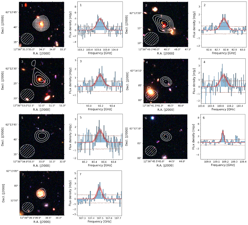
Figure 3: Emission line candidates with highest fidelity and $\mathrm{S/N}$. The left panels show the moment zero maps overlaid on the HST images (F160W/F850LP/F606W). Contours are spaced from $\pm 3\sigma$ up to $\pm 10\sigma$, spaced by $\pm 1\sigma$ (no negative contours are seen) and the synthesised beam is shown in the bottom left corner. The right panels show the peak pixel spectra and the rms noise (brown line), including Gaussian fits and $1\sigma$-uncertainties (red line and shading).

3 Analysis and Results

3.1 Line Search

We search the cubes for positive and negative line emission using matched filtering. Several codes have been developed in the context of different spectral scan surveys, including Findclumps (Walter et al., 2016; Decarli et al., 2019), Lineseeker González-López et al. (2019) and MF3D (Pavesi et al., 2018). All these codes have been found to perform qualitatively similarly, though differ somewhat in the way they perform the matched filtering and group the final list of candidates (e.g., González-López et al., 2019).

As our fiducial line search code, we use MF3D, which conducts the matched filtering on the $\mathrm{S/N}$ cube using spatial and spectral kernels of different sizes. We use a Gaussian kernel in frequency space, with widths ranging from 3 to 18 channels, corresponding to line widths of about 75 to 500 km s^-1 (FWHM). We use a single-pixel (point-like) spatial kernel, as all sources are expected to be unresolved at the beam size.

We use the distribution of the negative lines (expected to be produced by noise), to estimate a ‘fidelity’ of the positive line signal as a function of $\mathrm{S/N}$. The fidelity is computed per kernel ($\sigma$) by taking the ratio of the number of positive and negative lines ($N_{\rm pos}$, $N_{\rm neg}$) in bins of $\mathrm{S/N}$,

$$F(\mathrm{S/N},\sigma)=1-\frac{N_{\rm neg}(\mathrm{S/N},\sigma)}{N_{\rm pos}(\mathrm{S/N},\sigma)}$$ (1)

To mitigate the effect of low-number statistics on the estimate of $N_{\rm neg}(\mathrm{S/N},\sigma)$, we fit the counts with a tail of a Gaussian function centered at zero (as in González-López et al. 2019; Decarli et al. 2019, 2020). We finally compute a smooth estimate of the $F(\mathrm{S/N})$ at fixed $\sigma$ by fitting an error function shape to Equation 1 (cf. Walter et al., 2016). As the number of sources detected in the individual cubes is rather limited for a given kernel width, the estimate of the fidelity at a fixed $\mathrm{S/N}$ is uncertain (except at the tails of the distribution, close to zero and unity fidelity). To mitigate this effect, we combine the line search results in S/N-space and compute a single fidelity estimate for a given kernel width for all cubes combined. This is equivalent to performing the analysis on the combined cube, as is typically done. This provides a more robust estimate of the fidelity, though we still caution against over-interpreting the exact fidelity values in the intermediate range.

For the final catalog we only consider lines candidates with a $\mathrm{S/N}>4$ (also when remeasured with a Gaussian fit, see § 3.5), a $F>0.2$ (consistent with earlier work), and that lie in the area of the mosaic where the sensitivity is above 40% of the peak sensitivity. This leaves a total of 23 sources, all of which have a $\mathrm{S/N}\geq 5$ due to the fidelity cut being more stringent than the $\mathrm{S/N}$ cut, and that lie within $\sim 50\%$ of primary peak sensitivity. There is a relatively sharp drop in fidelity below $\sim 0.7$ and the majority of the sources lie at lower fidelity- and $\mathrm{S/N}$-end. We list the highest fidelity sources, with $F\geq 0.7$, in Table 3, which have a $\mathrm{S/N}\geq 5.85$.

We estimate the completeness of our line search by injecting simulated emission lines into the cubes and determining what fraction is recovered by our line search procedure. We assume a 3D Gaussian profile for the simulated lines, which matches shape of the beam for each cube in the spatial directions. We draw 1000 sources from a uniform distribution in peak flux and FWHM line width, ranging from 0 to 3 mJy and 0 to 800 km s^-1 respectively. The sources are then injected uniformly across the cubes in the area above 50% of the peak sensitivity. We perform the line search in the same manner as described above and define the completeness ($C$) as the fraction of the injected sources that are recovered for a given line width and peak flux. We repeat the experiment 5 times for each cube to increase statistics to a total of 5000 lines per sideband (20.000 simulated lines in total). The resulting completeness fractions are shown in Fig. 11 in Appendix A. In the end, we find the completeness corrections are minor, as the uncertainties are dominated by the sample purity (fidelity) and not completeness.

We cross check the line candidates found with MF3D against those found by Findclumps and Lineseeker. Overall, we recover the same high-$\mathrm{S/N}$ and -fidelity candidates with all the codes (though there are differences in the absolute $\mathrm{S/N}$, due to the different methods), while there are increasing numbers of candidates found by only a subset of the codes at lower $\mathrm{S/N}$. Similar conclusions were also reached by Decarli et al. (2019) and González-López et al. (2019). We further assess the impact of the line-search code used in Appendix A, where we show we recover the same CO luminosity functions if we use the line candidates from Findclumps in favor of MF3D.

3.2 Counterpart association

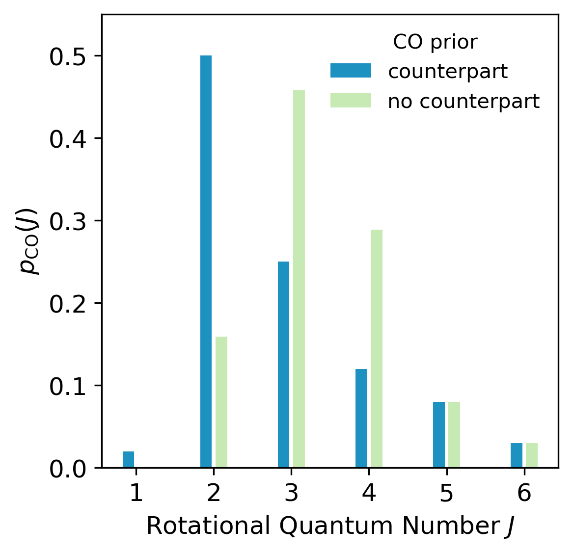
Figure 4: CO line prior used for the redshift associations. The prior for sources with an (HST) counterpart is based on the observed CO line distribution from ASPECS (Decarli et al., 2020). For the sources without counterpart, we use a line distribution based on the redshift distribution of optically-faint submillimeter galaxies from Smail et al. (2021) in combination with a typical CO ladder (Danielson et al., 2011; Boogaard et al., 2020).

We identify the redshifts of the candidates from the line-search by exploiting the extensive multi-wavelength data that is available over the HDF-N as compiled by the CANDELS and 3D-HST surveys (Grogin et al., 2011; Koekemoer et al., 2011; Brammer et al., 2012; Skelton et al., 2014; Momcheva et al., 2016), including spectroscopic redshifts (e.g. Barger et al., 2008), as well as the Herschel data (Elbaz et al., 2011).

While for the brightest and/or lower-redshift galaxies the counterpart association is often clear, the relatively large beam of the NOEMA data (compared to typical galaxy sizes) can sometimes lead to ambiguities in the association. There may be multiple galaxies near the peak of the emission or, especially at lower S/N, the peak of the emission may be offset from the position of the counterpart. Moreover, the counterpart may not be detected in the optical/near-infrared imaging at all.

To deal with these uncertainties, we assign a redshift probability for every line candidate, based on the photometric redshift distributions of galaxies in the vicinity, weighted by their relative distance to the source. We also include a ‘dark’ solution, in which there is no optical/NIR photometric counterpart. We use the photometric redshift distributions that are derived with eazy by 3D-HST (Brammer et al., 2012; Skelton et al., 2014; Momcheva et al., 2016). We take a prior on the separation between the line candidate and the photometric counterpart in the form of a Gaussian with a 2” FWHM (about half the beam size), i.e., a radial down-weighting of sources at a larger separation from the line position.

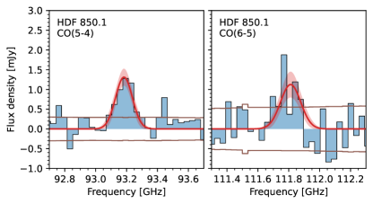
Figure 5: Spectra of CO(5-4) and CO(6-5) in HDF 850.1, binned by a factor 5. Both lines are detected, but CO(6-5) only at lower S/N (below the line-search threshold). A joint Gaussian fit to both lines is shown in red, yielding integrated fluxes of $S_{\mathrm{CO(5-4)}}=0.58\pm 0.10$ Jy km s^-1, $S_{\mathrm{CO(6-5)}}=0.49\pm 0.14$ Jy km s^-1, and a line width of $412\pm 72$ km s^-1 at $z=5.184\pm 0.001$.

Because it is well known that not all CO transitions are observed in equal numbers at fixed observing frequency, we take into account different prior probabilities on the CO line identification. For the sources with a photometric counterpart, we adopt a prior that is loosely based on the line-flux distribution from ASPECS at 3 mm (Decarli et al., 2020). For the sources without a photometric counterpart, we adopt the redshift distribution of optically-faint submillimeter galaxies ($K$-faint) as found by Smail et al. (2021) and convert it to a CO line distribution in $J$ assuming a fiducial CO ladder based on the typical integrated line flux ratios in SMGs (Danielson et al. 2011, cf. Boogaard et al. 2020). Both CO line priors are shown in Fig. 4. Above a redshift of $\sim 3$ there is some ambiguity in the line identification, where multiple lines from CO and $\mathrm{[C\,\textsc{i}]}$ are potentially present in the spectrum. For the identification, we assume that the line is always the strongest line visible at the respective redshift, and check for fainter lines afterwards. This concerns $\mathrm{[C\,\textsc{i}]}$(1–0), that is typically weaker than CO(4–3) (e.g., Valentino et al., 2020), and the $J>6$ CO lines, that are rarely significantly stronger than CO(6–5) (Carilli & Walter, 2013). Effectively, this means that all lines are assumed to be CO with $J\leq 6$. We discuss the impact of these priors on the final results in more detail in Appendix A.

The redshift probability for a line candidate observed at a frequency $\nu$ and position $s$ is given by:

$$p(z|\nu,s)\propto\sum_{i}\left[p_{i}(z|s_{i})p(z|\nu)p(s_{i}|s)\right]+p_{d}(z|\nu,s_{d})p(s_{d}|s),$$ (2)

where the sum is taken over all galaxies that lie within a 6” diameter circle (i.e., significantly larger than the beam and typical galaxy sizes). Here $p_{i}(z|s_{i})$ is the photometric redshift distribution for galaxy $i$ at position $s_{i}$, $p(z|\nu)$ is the redshift prior determined by the CO line prior and the observed frequency, and $p(s_{i}|s)$ is the radial weighting that depends only on the absolute separation $|s_{i}-s|$. The last term represent the no-counterpart or ‘dark’ case, where $p_{d}(z|\nu,s_{d})$ is the associated (prior) redshift probability distribution and $p(s_{d}|s)$ accounts for the relative weight that is given to the no-counterpart solution. For the latter we assume the value of the radial weighting at $2^{\prime\prime}$, which means the no-counterpart solution gets a larger weight than solutions with a counterpart for separations larger than $2^{\prime\prime}$. The overall probability is normalised to unity for each line candidate, depending on the number of photometric counterparts and their radial weight.

The $p(z)$ distribution for the top sources are shown in Fig. 13 in Appendix B. We cross-check the solutions for the highest fidelity sources with the additional spectroscopic redshifts from literature and find that the $p(z)$ solutions are in perfect agreement with the known spectroscopic redshifts analysis in all cases. The redshifts and associated line identifications are reported in Table 3.

We find the majority of lines (4/7) are CO(2–1) emitters with redshifts $1<z<2$. Three out of 4 are supported by a spectroscopic redshift, while for ID.6 the $p(z)$ solution contains more than 90% of the total probability. The high number of CO(2–1) emitters is very consistent with the findings from ASPECS, where the majority of lines were from CO(2–1) (roughly 60%), followed by CO(3–2) (roughly 30%), cf. Fig. 4. There is no CO(3–2) emitter with an unambiguous redshift identification, though the redshift probabilities of both sources with a broader $p(z)$ peak at $J=3$. We detect CO(5–4) in HDF 850.1 and its spectrum also reveals reveals CO(6–5), albeit at lower fidelity and $\mathrm{S/N}$ (below the line-search threshold), shown in Fig. 5.

An alternative method to identify the CO line redshifts is to use the long-wavelength dust spectral energy distribution and compare the inferred dust temperature of the line emitter to the dust temperature distribution of sources with known redshifts (e.g., Weiß et al., 2013; Strandet et al., 2016). To this end, we cross-match our line list to the Herschel catalog from Elbaz et al. (2011). We find a clear Herschel counterpart within $1^{\prime\prime}$ for all sources, with the exception of IDs 4, 5 and 6, hence no additional constraints on their potential redshift can be derived in this way.

3.3 Comparison to earlier PdBI observations

We re-examine the 16/21 candidate emission lines from the earlier PdBI observations in the HDF-N (Walter et al., 2014; Decarli et al., 2014, with a similar average rms of $\sim 0.55$ mJy per 9 MHz channel) that fall within the present frequency coverage (i.e., excluding their ID.1, 2, 19, 20 and 21). We confirm their ID.3 and ID.8 (HDF 850.1), which are recovered as ID.2 and ID.3 in the present line search. In addition, we also confirm ID.17, which is recovered at low fidelity in the present line search, but is robust, corresponding to CO(6–5) in HDF 850.1 (see Fig. 5). For the remaining original line candidates no significant emission is identified in the new observations.

3.4 Continuum

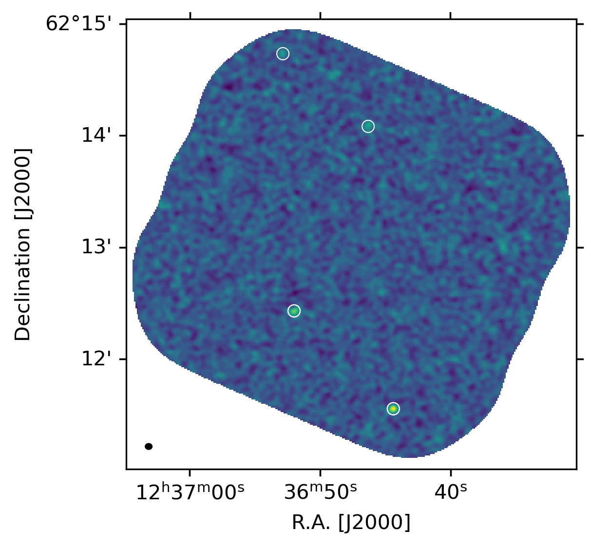
Figure 6: Continuum map at 97.8 GHz before applying the mosaic primary beam correction. The rms noise is 11 $\mu$Jy beam^-1 and the beam size is shown in the bottom left corner. The brightest sources are marked with circles (cf. Fig. 7).

Table 4: Properties of continuum sources.

ID	R.A.	Decl.	S/N	F	PB	$S_{\nu,3mm}$	$z$
	(J2000)	(J2000)				($\mathrm{\mu Jy}$)
(1)	(2)	(3)	(4)	(5)	(6)	(7)	(8)
C1	12:36:44.38	+62:11:33.5	11.01	1.00	0.78	$148\pm 22$	1.013
C2	12:36:52.00	+62:12:26.0	7.55	1.00	0.99	$110\pm 23$	5.184
C3	12:36:46.31	+62:14:05.0	4.74	0.92	0.93	$92\pm 17$	0.961
C4	12:36:52.86	+62:14:44.0	4.32	0.81	0.52	$103\pm 25$	0.321

Note. — (1) Continuum ID. (2–3) Right ascension and declination. (4) S/N from matched filtering (5) Fidelity. (6) Mosaic sensitivity relative to peak at the source position. (7) Flux density at 3 mm. (8) Spectroscopic redshifts from Barger et al. (2008), except for C2 (HDF 850.1; Walter et al., 2012, this work).

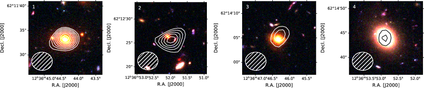
Figure 7: Continuum sources overlaid on the HST imaging (F160W/F850LP/F606W). Contours are spaced from $\pm 3\sigma$ up to $\pm 10\sigma$, spaced by $\pm 1\sigma$ and the synthesised beam is shown in bottom left corner. The second continuum source is HDF 850.1, the other three are all radio galaxies at $z\leq 1$ (see references in text).

The 3 mm continuum map is shown in Fig. 6, prior to the mosaic primary beam-correction (i.e., with flat noise). We search for sources in the dirty continuum map using matched filtering in the same way as for the cubes, but with a 1-channel spectral template. We detect four continuum sources with a fidelity above 0.8 ($\mathrm{S/N}>4.3$). We Hogbom clean the cube around the brightest sources from the line search down to $2\sigma$. We measure the fluxes in the cleaned image by fitting 2D Gaussians using imfit in casa. The properties of the sources and measured fluxes are listed in Table 4.

We show HST cutouts of the continuum sources in Fig. 7. The second brightest source corresponds to HDF 850.1. The other three sources are all identified as known (radio) galaxies detected at 1.4, 5, 10 and 34 GHz (Morrison et al., 2010; Owen, 2018; Gim et al., 2019; Murphy et al., 2017; Algera et al., 2021) showing AGN signatures in their X-ray (Xue et al., 2016) and/or radio emission (Algera et al., 2021), with known spectroscopic redshifts $\leq 1$ (Barger et al., 2008). No bright lines fall within the frequency range of the mosaic at the redshift of these three sources (cf. Table 1). The 3 mm number counts at $5\sigma$ of $N(>0.09\,\mathrm{mJy})\approx 850\,\mathrm{deg}^{-2}$ (no completeness or flux-boosting correction correction) are in good agreement with the recent estimates from Zavala et al. (2021).

3.5 Properties of sources

We fit the lines recovered in the line search with a Gaussian line profile using lmfit (Newville et al., 2019). The resulting line fluxes, frequencies, and widths are reported for the high-fidelity sources in Table 3. We do not apply any flux boosting corrections, as the completeness simulations (§ 3.1) show that this only has a minor impact on the line flux at the S/N levels under consideration. As in Decarli et al. (2020), we also do not correct the line fluxes for the impact of the increasing temperature of the Cosmic Microwave Background (CMB) with redshift, though note these would only significantly decrease the observed line flux at relatively low intrinsic excitation temperatures. We refer the reader to Decarli et al. (2020) for a more in-depth discussion of both topics. We compute the line luminosities ($L^{\prime}$) in units of K km s^-1 pc² (e.g., Solomon et al., 1992; Carilli & Walter, 2013) for each of the the various redshift solutions from the $p(z)$ analysis, which are used for the computation of the CO LFs.

3.6 Luminosity Function Analysis

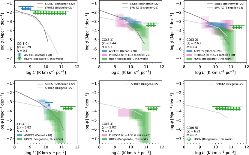
Figure 8: CO luminosity functions in the HDFN (green boxes). Each panel indicates the CO transition and mean redshift, as well as the mean number of sources that entered the luminosity function (from 5000 realisations). The blue boxes show the results from ASPECS (Decarli et al., 2020) and the pink boxes from PHIBSS2 (Lenkić et al., 2020).

The luminosity functions are computed following the approach of Decarli et al. (2016a, 2019, 2020), but taking all 23 sources (§ 3.1) into account for the luminosity functions of all the different lines, with a weight depending on their $p(z)$ solution. The exception to this are the high-fidelity sources with a spectroscopic redshift, for which we only include the actual redshift with a fidelity of unity.

The luminosity function for a certain transition is then defined as:

$$\phi(\log L^{\prime})~{}[\mathrm{Mpc}^{-3}\,\mathrm{dex}^{-1}]=\frac{1}{V\Delta(\log L^{\prime})}\sum_{i=1}^{N}\frac{F_{i}}{C_{i}}.$$ (3)

Here $\phi$ is the number of sources per comoving Mpc³ in an interval of $\log L^{\prime}\pm 0.5\log L^{\prime}$, $V$ is the volume over which a transition is detectable, $\Delta(\log L^{\prime})$ is the bin width, and $F_{i}$ and $C_{i}$ are the fidelity and completeness for a given transition. To construct the luminosity functions, 5000 independent realisations are created, where in each realisation the line luminosities are varied within errors. The number of sources and associated $1\sigma$ Poissonian confidence intervals (Gehrels, 1986) are computed in 0.5 dex bins, unless a bin contains less than one source on average, in which case a $3\sigma$ upper limit is provided. The resulting counts and uncertainties are finally scaled by the completeness corrections, divided by the volume and averaged over the realisations. Following earlier work, the luminosity functions are computed five times with offsets of 0.1 dex (which are therefore not independent), to expose the intra-bin variations given the modest statistics.

The luminosity functions in the HDFN are shown in Fig. 8 for CO(1–0) up to CO(6–5) and are tabulated in Table 7. We compare these to the recent luminosity functions for the HUDF determined by the ASPECS Large Program (Decarli et al., 2019, 2020). These are also determined from a spectral scan at 3 mm, over almost exactly the same redshift interval (cf. Fig. 2), but probe down to fainter luminosities over a $\sim 2.5\times$ smaller volume. We also show the LFs derived from background sources in the PHIBSS2 fields (Lenkić et al., 2020) for the redshift ranges that are reasonably close to those from NOEMA HDFN and ASPECS.

We compare the observed LFs to the recent theoretical predictions from the SIDES (Béthermin et al., 2022) and Spritz (Bisigello et al., 2022) simulations. In brief, both simulations use empirical prescriptions for the IR luminosity and CO-to-IR scaling relations. SIDES simulates the galaxy population using a semi-analytical model that that is coupled to the stellar mass of dark matter halos determined via abundance matching on a dark matter-only light-cone from the Bolshoi-Planck simulations (Rodríguez-Puebla et al., 2016), while Spritz is a fully empirical model that is based on the observed galaxy stellar mass and IR luminosity functions.

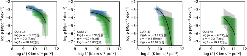
Figure 9: Schechter fits to the CO luminosity functions of the HDFN (green boxes) + ASPECS (blue boxes). Each panel indicates the CO transition and the fit parameters (cf. Table 5).

In both the local universe and at higher redshift, the (lower-$J$) luminosity functions have been found to be reasonably well described by Schechter (1976) functions (e.g., Saintonge et al., 2017; Fletcher et al., 2020; Riechers et al., 2019; Decarli et al., 2019). Given the broad overall agreement between the LF’s from the HDF-N and HUDF, further discussed in § 3.6, we perform a joint fit using a Schechter function in logarithmic units (e.g., Riechers et al., 2019):

$$\log\phi=\log\phi_{*}+\alpha\log\left(\frac{L^{\prime}}{L^{\prime}_{*}}\right)-\frac{1}{\ln 10}\frac{L^{\prime}}{L^{\prime}_{*}}+\log(\ln 10)$$ (4)

Here $\phi_{*}$ is the normalisation defining the overall density of galaxies at the characteristic luminosity $L^{\prime}_{*}$ (in the same units as Equation 3) and $\alpha$ is the faint-end slope. We only fit uncorrelated bins for each dataset, i.e., one-fifth of bins evenly spread across the full range probed, to avoid underestimating the uncertainties (note that we find the same median posterior values if we would fit all the bins, but with narrower posteriors). We also chose not to fit the PHIBSS2 data, as they are not derived consistently with the redshift intervals of the other surveys. As we do not provide new constraints on the faint-end, we fix the slope $\alpha=-0.2$ following Decarli et al. (2020), that is consistent with the local value (Saintonge et al., 2017). We take uniform priors, where $-6\leq\log\phi_{*}\leq-2$ and $8.5\leq\log L^{\prime}_{*}\leq 11.5$, and sample the posterior on the parameters using nested sampling with Ultranest (Buchner, 2021). The resulting fits are shown in Fig. 9 and the marginalised estimates for the parameters are tabulated in Table 5.

As it appears that CO(4–3) may not be well described by a single Schechter function, we also explored fitting two Schechter functions to the $J=2$, 3 and 4 LF’s (with broader priors of $-9<\log\phi_{*,1,2}<-1$ and $8.0\leq\log L^{\prime}_{*,1,2}\leq 12.0$, and the requirement that $\log L_{*,1}<\log L_{*,2}$). However, we find that in all cases the ratio ($K$) of the Bayesian evidence ($Z$) supports the single Schechter fits, with $K=Z_{\rm double}/Z_{\rm single}\leq 0.5$ (Jeffreys, 1961).

Table 5: Schechter function parameters posterior percentiles for different CO transitions.

Transition	$\langle z\rangle$	$\log\phi_{*}$	$\log L^{\prime}_{*}$
		(Mpc-3 dex${}^{-1})$	(K km s-1 pc2)
(1)	(2)	(3)	(4)
CO(2–1)	1.439	$-3.32_{-0.21}^{+0.20}$	$10.46_{-0.23}^{-0.41}$
CO(3–2)	2.628	$-3.96_{-0.23}^{+0.27}$	$10.83_{-0.39}^{-0.44}$
CO(4–3)	3.821	$-3.17_{-0.38}^{+0.35}$	$10.04_{-0.24}^{-0.56}$
CO(5–4)	5.016	$-4.23_{-0.72}^{+1.13}$	$10.43_{-0.59}^{-0.71}$

Note. — See Equation 4. We fix $\alpha=-0.2$.

4 Discussion

4.1 CO luminosity functions

The large volume of the NOEMA survey provides new constraints on the bright end of the CO LF, as shown in Fig. 8. Compared to ASPECS, the roughly $3\times$ shallower observations over $2\times$ the area extend the overall constraints past the knee of the LF, while reaching comparable constraints near the knee.

We find a lower luminosity density in the overlap regions of the LF in the HDF-N compared to the HUDF, of roughly 0.15 dex for CO(2–1) and 0.4 dex for CO(3-2). It is not immediately clear where these differences come from, but they do not appear to be methodological (Appendix A). More likely they are due to field-to-field variance. It is known that there is an overdensity in the HUDF at $z\sim 1.1$ that may bias the CO(2–1) measurements from ASPECS high (Boogaard et al., 2019). It is unclear if similar over- or underdensities affect the comparison of the CO(3–2) LF, though we cannot confidently identify the same fraction of CO(3–2) emitters as were found in the HUDF. Even larger variations are seen when comparing to the LFs from PHIBSS2. This suggest that the variations seen between the fields can be attributed to cosmic variance. Interestingly both SIDES and Spritz seem to predict a lower luminosity density for CO(2–1) than is observed in both fields, making it less clear whether this is due to cosmic variance (Béthermin et al., 2022) or a missing ingredient in the models. Taken together, the combined measurements from the HDF-N and HUDF are (still) reasonably well described by a single Schechter function (Fig. 9). The joint fits provide improved constraints on the overall shape of the LFs, which now explicitly take into account the measured cosmic variance between the fields.

For CO(4–3), it appears we find a larger number of sources at the bright end than may be expected from an extrapolation from ASPECS. One should note the total number of sources entering the LF here is very limited: there are only 1 and 2 independent LF bins for ASPECS and the HDF-N respectively, with very few sources, hence the differences could simply be due to noise and low-number statistics. Given there are no CO lines with spectroscopic confirmation entering this bin, it is also more sensitive to the assumed priors, and only upper limits can be derived if one limits to the top-sources (see Appendix A for more details). We do find that the bright end of the CO(4–3) LF is consistent with the predictions from both SIDES and Spritz, while the models predict a lower luminosity density than is observed towards the fainter end (Béthermin et al., 2022; Bisigello et al., 2022). While it appears there is a tantalising break in the CO(4–3) LF we find it is not statistically significant (see § 3.6) and the differences could again be caused by cosmic variance. If real, such a break could be caused by a rapid change in the average excitation between the faint and bright end of the LF at these redshifts, though such a scenario is not seen in the simulations, which are otherwise consistent with the LF in the HDF-N.

As the cosmological deep fields are biased against having very low-redshift galaxies in the foreground, we only provide a $3\sigma$ upper limit on the CO(1–0) luminosity function at the bright end of $\log\phi\,[\mathrm{Mpc}^{-3}\,\mathrm{dex}^{-1}]\leq-1.9$. This is somewhat more stringent than that of ASPECS due to the increased volume. There are no high-fidelity sources contributing to CO(6–5) at the highest redshifts, implying a $3\sigma$ upper limit at the bright end of the luminosity function of $\log\phi\,[\mathrm{Mpc}^{-3}\,\mathrm{dex}^{-1}]\leq-3.6$. We do note that the eazy photometric redshifts do not fully cover the redshift range spanned by CO(6–5), which implies some signal may be lost in this bin (though the majority of the signal is expected to come from the no-counterpart sources), hence the constraints should be viewed as conservative. The same upper limit also extends to the higher-$J$ lines, nearly independent of transition (cf. Fig. 8). For both CO(1–0) and CO (6–5), the upper limits are comfortably in agreement with theoretical models.

The original PdBI pointing (Walter et al., 2014; Decarli et al., 2014) was chosen specifically to include the bright sub-millimeter galaxy HDF 850.1 and hence could not provide constraints on the CO(5–4) LF. The full mosaic, however, is not chosen to include this source. Therefore, it now provides the first measurement of the CO(5–4) LF at $\langle z\rangle=5$. The constraints on the LF are still limited and subject to cosmic variance (given that the expected source density of galaxies like HDF 850.1 is $\lesssim 1$ for the area of the HDF-N survey, e.g., Zavala et al. 2021), but in overall agreement with the predictions from Spritz.

In contrast to the empirical models discussed above, Popping et al. (2019) have used the IllustrisTNG hydrodynamical simulations (Weinberger et al., 2017; Pillepich et al., 2018) and the Santa Cruz semi-analytical model (Somerville & Primack, 1999; Somerville et al., 2001) to demonstrate that simulations which model galaxies from first principles generally do not reproduce the observed luminosity functions, unless the HUDF is a strong outlier (i.e., only a small fraction of the various realisations agreed with the HUDF). The result that our best-constrained CO LFs in the HDF-N, CO(2–1) and CO(3–2), do not deviate strongly from those the HUDF implies there is increasing tension with the simulations that predict significantly smaller amounts of molecular gas in galaxies on average (Popping et al., 2019). These simulated CO LFs are quite sensitive to the assumed prescription for the value of $\alpha_{\mathrm{CO}}$, that is needed to convert the simulated molecular gas mass function to a CO LF. While better agreement can be found by assuming significantly lower average values of $\alpha_{\mathrm{CO}}\lesssim 1$, tension then still remains in matching the observed faint- and bright end of the mass and luminosity functions simultaneously (e.g., Popping et al., 2019; Dave et al., 2020).

4.2 Cosmic molecular gas density and cosmic variance

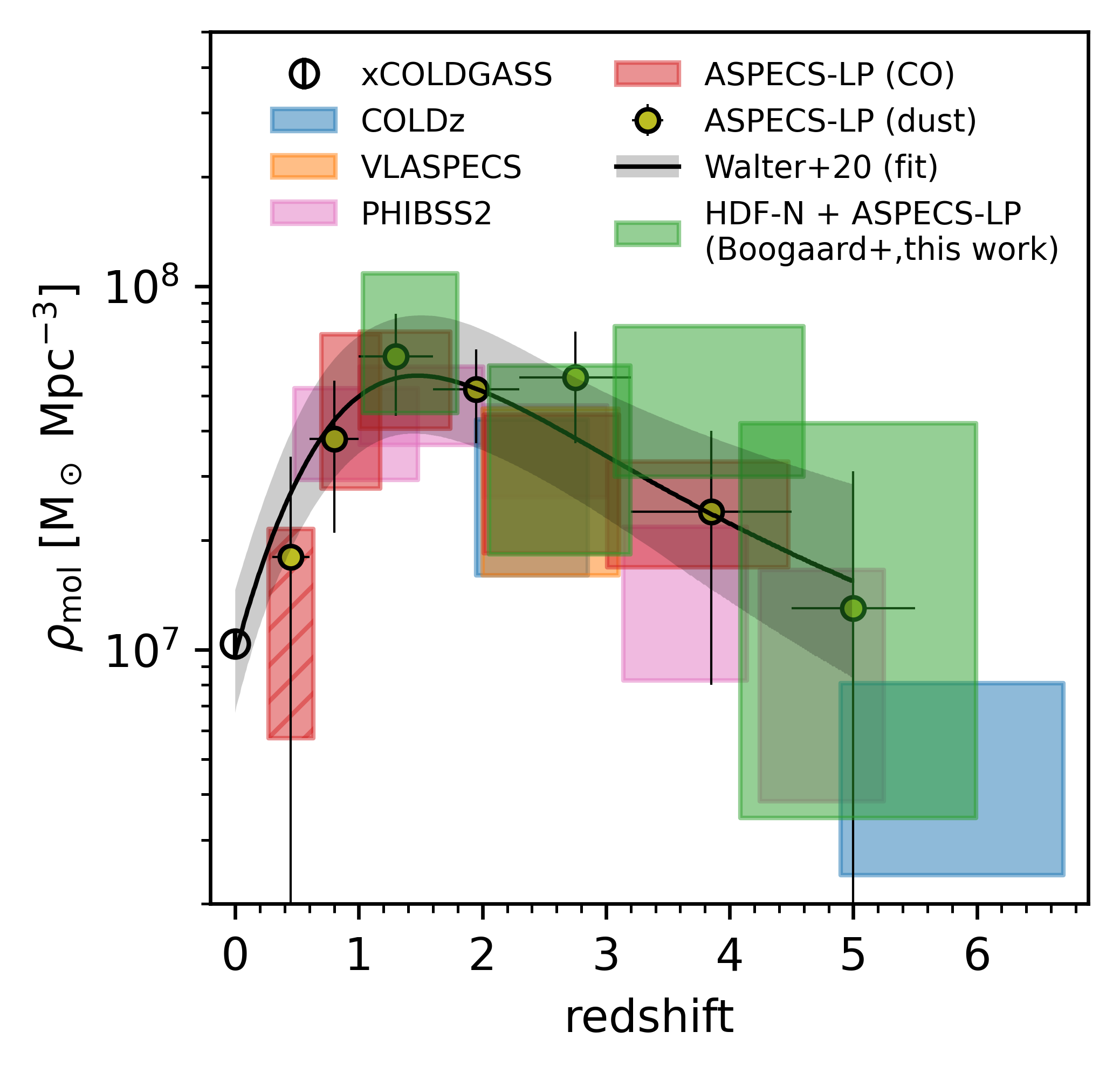
Figure 10: Cosmic molecular gas density from integrating the CO luminosity function fits for the HDF-N + HUDF (green boxes). We compare this to the local measurements from xCOLDGASS (Fletcher et al., 2020), COLDz in COSMOS and GOODS-N (Pavesi et al., 2018; Riechers et al., 2019), VLASPECS in the HUDF (Riechers et al., 2020), PHIBSS2 background sources (Lenkić et al., 2020), and the measurements from ASPECS in the HUDF (Decarli et al., 2019, 2020), incl. the dust continuum stacking (Magnelli et al., 2020). The gray line shows the join fit to all the literature data from Walter et al. (2020). The joint measurements confirm a rise of the cosmic molecular gas density from the local universe by a factor 4.5–11$\times$ to $z\sim 1.5$ and subsequent decline out to higher redshift, with slightly larger uncertainties reflecting the field-to-field variance between the HUDF and HDF-N.

The evolution of the cosmic molecular gas density is determined from the CO LFs at different redshifts. We combine the constraints from NOEMA in the HDF-N and ASPECS in the HUDF, by integrating the Schechter fits to both surveys down to the lowest $L^{\prime}$ probed in the data (i.e., we do not extrapolate the faint end). This is consistent with earlier work and the integral should trace the bulk of the molecular gas mass given that the knee of the luminosity function is well sampled. Indeed, the stacking results at $1\leq z<2$ from ASPECS (Inami et al., 2020) imply that there is not a large amount of gas mass missed at fainter luminosities. To convert the observed CO emission to a gas mass one needs to adopt a CO-to-molecular gas conversion factor, $\alpha_{\mathrm{CO}}$ (including He), and average excitation correction that is representative for galaxies around the knee of the LF. We assume an $\alpha_{\mathrm{CO}}=3.6$ $\mathrm{M}_{\odot}$(K km s^-1 pc²)^-1 (Daddi et al., 2010; Bolatto et al., 2013), mainly to be consistent with earlier work, but note all results can simply be linearly rescaled to a different $\alpha_{\mathrm{CO}}$. For the excitation, we adopt the average values derived for galaxies at $z<2$ and $z>2$ from Boogaard et al. (2020), with $r_{J1}=[0.75,0.80,0.61,0.44]$ for $J=[2,3,4,5]$. These ratios have been derived from the flux-limited sample of CO-emitters from the ASPECS survey and were also used for the ASPECS measurements (Decarli et al., 2020). Note the assumed $r_{51}$ is also reasonably similar to the excitation measured in HDF 850.1, with $r_{52}\approx 0.47\pm 0.15$ (Walter et al., 2012, assuming that CO(2–1) will be highly excited in the intense starburst, even if only from the high CMB temperature at this redshift). The resulting cosmic molecular gas densities are shown in Fig. 10 and tabulated in Table 6.

Table 6: Cosmic molecular gas density from the NOEMA HDF-N + ASPECS HUDF ($1\sigma$ range).

Transition	$\langle z\rangle$	$\log\rho_{\rm mol}$
		(M⊙ Mpc${}^{-3})$
(1)	(2)	(3)
CO(2–1)	1.4389	7.65, 8.04
CO(3–2)	2.6276	7.26, 7.78
CO(4–3)	3.8210	7.48, 7.89
CO(5–4)	5.0156	6.54, 7.62

Note. — The molecular gas densities, $\rho_{\rm mol}$, are given as the 16th and 84th percentiles ($1\sigma$).

The new constraints on the cosmic molecular gas density at $1<z<1.8$ and $2<z<3.1$ are in good agreement with earlier measurements, including those derived (independently) from the dust continuum in the HUDF (Magnelli et al., 2020), as well as the constraints from lower-$J$ transitions at the same redshift in COSMOS, GOODS-N and the HUDF (Pavesi et al., 2018; Riechers et al., 2019, 2020). The uncertainties are similar or in fact somewhat larger than the measurement from ASPECS alone at $\langle z\rangle=1.4$, which reflects the impact of cosmic variance on the LF and subsequent $\rho_{\rm mol}$ measurements. The combined constraints confirm the rise in the cosmic molecular gas density from redshift zero out to $z\sim 1.5$, with a factor between 4.5–11$\times$, and a subsequent decline out to higher redshift.

The relatively high $\rho_{\rm mol}(3<z<4.5)$ is because the best-fit Schechter function appears to somewhat overestimate the knee of the LF. As stated in § 3.6, the constraints on the CO(4–3) LF are rather limited, and we conclude that there is still significant uncertainty in the detailed shape of the LF as well as the molecular gas density at these redshifts. Indeed, the measurements from (Lenkić et al., 2020) fall significantly below the average (Walter et al., 2020). Alternatively, it could be that the average excitation is higher than assumed, though this is unlikely to explain the full discrepancy. Further analysis is needed to better constrain the luminosity density at these redshifts (cf. Boogaard et al., 2021b). We also show the constraints on $\rho_{\rm mol}(4<z<6)$ based on the CO(5–4) LF. The large uncertainties are due to the limited constraints on the LF, though overall the value are consistent with early measurements. The scatter around the average excitation is expected to be significantly larger for the higher-$J$ lines that trace warmer and denser gas, which makes the estimate of the associated total gas mass from these lines more uncertain.

The new measurements from the NOEMA HDF-N survey provide an important complement to the earlier measurements in other fields. For both the luminosity function and molecular gas density, perfect agreement is not expected because these are determined from different fields. The overall good agreement between the LFs in the HDFN and HUDF, especially for CO(2–1) and CO(3–2) implies that the impact of cosmic variance on these LFs is not more severe than previously estimated (Popping et al., 2019; Decarli et al., 2020). Indeed, while the area-on-sky of the spectral scan surveys are typically modest, the broad redshift coverage implies that substantial volumes are probed (cf. Table 1), mitigating the impact of field-to-field variance (Popping et al., 2019). The combined measurements from the HDF-N and HUDF presented here now fold in the uncertainties due to cosmic variance between the two fields directly.

5 Conclusions

This paper presented an 8.5 arcmin² NOEMA survey of the Hubble Deep Field North (HDF-N), that scans nearly the complete 3 mm band (from 82–113 GHz) band in 45 pointings, to identify for molecular line emission in distant galaxies, measure the CO luminosity functions (LF), and constrain the cosmic molecular gas density ($\rho_{\rm mol}$) out to $z\sim 6$. The main conclusions of this study are as follows.

1. We search for line candidates in the cube via matched filtering and determine a redshift probability distribution, $p(z)$, for each of the line candidates exploiting the existing photometric redshift distributions of nearby counterparts in combination with a CO redshift prior, including a no-counterpart solution. Out of the larger sample of candidates, we identify 7 high-confidence line emitters (with $\mathrm{S/N}\geq 5.85$ and fidelity $F>0.7$). Four are CO(2–1) emitters at $1<z<2$ (of which three spectroscopically confirmed), two have a broader $p(z)$ but are most likely CO(3–2) emitters at $2<z<3$, and the final source is HDF 850.1, a well-known starburst galaxy at $z=5.184$ (Walter et al., 2012) detected in both CO(5–4) and CO(6–5).

2. We detect four high-confidence 3 mm continuum sources. One is HDF 850.1, while the other three are all identified as known radio galaxies with spectroscopic redshifts $z\leq 1$.

3. The larger area and significant depth of the NOEMA HDF-N survey compared to earlier studies provides the first constraints on the bright end of the CO LFs for $J=2$ up to $5$ at $1<z<6$, extending the existing LF measurements up to $z\sim 4$ from the knee upwards. We find a lower density in the overlap region near the knee of the CO(2–1) and CO(3–2) LFs in the HDF-N compared to the HUDF (from ASPECS) of $\sim 0.15$ and 0.4 dex, respectively. We find tentative evidence for a higher CO(4–3) luminosity density at the bright end than expected from extrapolations of earlier surveys, though in good agreement with simulations. Finally, we provide the first constraints on the CO(5–4) LF at $\langle z\rangle=5$.

4. We perform a joint analysis of the LFs in the HDF-N and HUDF (from ASPECS) and find that they are well described by Schechter functions up to at least $J=3$. Given that the constraints were determined from two completely independent fields, this suggests that the current measurements of the LFs and subsequently the cosmic molecular gas density are not strongly affected by cosmic variance.

5. The agreement between the HDF-N and HUDF poses some challenges for simulations that model galaxies from first principles, that (under the assumption of an $\alpha_{\mathrm{CO}}$) generally predict lower values for the CO LFs than are observed.

6. We integrate the combined HDF-N and HUDF LFs to provide revised constraints on the molecular gas density from the joint fields. The uncertainties on $\rho_{\rm mol}$ from the joint determination are similar and in some cases even slightly larger. The latter is a direct consequence of the field-to-field variance which is now reflected in the measurements. We find very good agreement with earlier surveys for $\rho_{\rm mol}(1.0<z<1.8)$ and $\rho_{\rm mol}(2<z<3.2)$ and $\rho_{\rm mol}(4<z<6)$. The results show that the cosmic molecular gas density increases by a factor 4.5–11 from redshift 0 to $z\sim 1.5$, in agreement with previous measurements including independent measurements from the dust continuum.

The independent constraints from the NOEMA HDF-N survey provide important constraints on the cosmic variance in the CO LF compared to the other deep fields such as the HUDF. On-going efforts such as WIDE ASPECS are expanding the spectral scan surveys to even larger areas to further constrain the variance in the bright end of the CO LF (not covered by ASPECS). The key combination of depth and relatively large area of the NOEMA HDF-N survey is made possible by the increased sensitivity of the extra antennas and in particular the large instantaneous bandwidth, allowing to scan the entire 3 mm band in only 2 tunings. Future upgrades on NOEMA, such as the dual-band, full-band and multi-beam receivers, as well as the upcoming Band 2 and bandwidth upgrades for ALMA (Carpenter et al., 2022), would allow to constrain the evolution of the cosmic molecular gas density even further.

Appendix A Luminosity functions: impact of methodology, priors and completeness

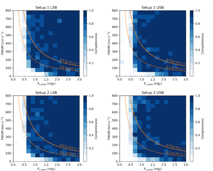
Figure 11: Completeness fractions for the four fields determined from injecting and recovering mock sources for a range of peak fluxes and line widths. The completeness is similar between the four sidebands, with a slightly higher completeness for the sidebands with lower rms. Overall, the completeness exceeds $90\%$ for integrated line fluxes above roughly 0.4 Jy km s^-1, being higher for narrower lines at fixed integrated flux.

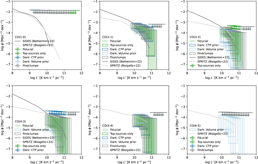
Figure 12: Impact on the CO LFs of different codes and assumptions, compared to the fiducial result from the paper (Fig. 8). The result obtained when using the line candidates from Findclumps (grey) are nearly identical to those obtained with MF3D, which is not only reassuring, but also supports the join analysis with ASPECS. Including only the top sources ($F>0.7$; dark green) leaves the $J=2$ and 5 LFs unchanged, but turns the constraints for $J=3$ and 4 into upper-limits only. The effect of changing the CO-line prior for the sources without counterpart to that of the sources with counterpart (dark blue) lowers the constraints on $J=4$, with minimal impact on the other lines. Using the volume prior used in (Decarli et al., 2019, light blue) instead, boosts the $J\geq 5$ LFs in favor of the lower-$J$ lines.

Table 7: CO luminosity functions.

	CO(2–1) at $\langle z\rangle=1.4389$	CO(3–2) at $\langle z\rangle=2.6276$	CO(4–3) at $\langle z\rangle=3.821$	CO(5–4) at $\langle z\rangle=5.0156$
$\log L^{\prime}_{*}$	$\log\phi_{*}$	$\log\phi_{*}$	$\log\phi_{*}$	$\log\phi_{*}$
(1)	(2)	(3)	(4)	(5)
10.05	-3.75, -3.16	$\cdots$	$\cdots$	$\cdots$
10.15	-3.79, -3.18	-4.44, -3.56	-5.05, -3.77	-4.94, -3.79
10.25	-3.99, -3.25	-4.43, -3.56	-4.98, -3.76	-4.84, -3.76
10.35	-4.09, -3.29	-4.50, -3.59	-5.03, -3.77	-4.85, -3.76
10.45	-4.01, -3.27	-4.68, -3.64	-5.21, -3.81	-4.90, -3.78
10.55	-4.22, -3.35	-5.04, -3.72	-5.61, -3.87	-5.09, -3.84
10.65	-4.57, -3.44	-5.63, -3.80	-6.26, -3.93	-5.70, -3.99
10.75	-4.67, -3.46	-6.20, -3.84	-7.24, -3.96	-7.40, -4.06
10.85	-4.85, -3.52	-6.54, -3.88	-7.86, -4.00	-15.81, -4.08
10.95	-6.26, -3.72	-7.16, -3.94	-8.48, -4.04	-17.02, -4.10
11.05	$\leq$ -3.18	-8.63, -3.97	-9.78, -4.06	-18.77, -4.10
11.15	$\cdots$	$\leq$ -3.42	$\leq$ -3.51	$\leq$ -3.55

Note. — (1) Center of the 0.5 dex-wide log luminosity bins. (2-5): Luminosity functions; the values denote the 16th and 84th percentile ($1\sigma$) or a $3\sigma$ upper limit.

In this section we investigate the impact of the methodology assumptions made for the CO-line identification and the subsequent impact on the luminosity function and cosmic molecular gas density. The completeness corrections as a function of line width and peak flux for each of the four cubes (discussed in § 3.1) are shown in Fig. 11. Overall, we find the completeness corrections are minor, as the uncertainties are dominated by the sample purity (fidelity) and not completeness.

While the different line-search code typically agree on the high-fidelity candidates, there are increasing differences in the exact number of candidates and their $\mathrm{S/N}$ and Fidelity for fainter lines. We therefore repeat the full CO LF analysis using the line candidates from Findclumps instead of MF3D. The results are shown in Fig. 12. Reassuringly, the CO LFs are effectively unchanged, with the only difference being a slightly higher count for the faintest bins. To check whether our computation of the LF is consistent with earlier work, we also recompute the CO(2–1) and CO(3–2) LFs from the ASPECS large program using the top 15 high-fidelity line candidates (González-López et al., 2019) and find that we recover the LFs from Decarli et al. (2019) perfectly (up to the completeness corrections at the faint end). We also investigate the impact of the prior on the sources with out a photometric counterpart. The first alternative we explore is to assume the same prior as for sources that do have a counterpart. This redistributes the lines towards the CO(2–1) bin, slightly reducing in the CO(3–2) bin, and loses constraints on the CO(4–3) bin (leaving only upper limits), whilst leaving CO(5–4) unchanged. We also explore take sources without counterpart into account with a weight purely proportional to the volume probed at each redshift (as in Decarli et al. 2019). This has the opposite effect, of reducing the $J\leq 4$ transitions more strongly towards lower-$J$, whilst slightly boosting the $J\geq 5$ luminosity functions, such that there are sufficient counts also in the $J=6$ LF (i.e., effectively more than one source).

In summary, we find the CO(2–1) and CO(5–4) luminosity functions are robust, because they are well-defined by the sources that have a confident identification, such that the prior assumptions (or different line search codes) have minimal impact on the final result to within uncertainties. Moreover, the impact on the (combined) $\rho_{\rm mol}$ constraints for these lines are negligible. For CO(3–2) and CO(4–3) somewhat larger variation is seen towards the faint end, while the bright end remains robust. Using only the top-fidelity sources, however, results in only upper limits on CO LFs for the latter two transitions.

Appendix B Redshift distributions

The redshift probability distributions (Equation 2) for the top candidates from Table 3 are shown in Fig. 13, except for HDF 850.1 which is known to have no photometric counterpart and a spectroscopic redshift of $z=5.184$ (Walter et al., 2012).

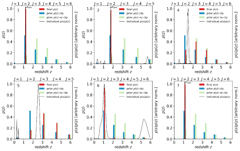
Figure 13: Redshift probability distributions, $p(z)$, for the top candidates (except HDF 850.1). The solid red bars show the final $p(z)$ and the other bars show the priors (cf. Fig. 4). The black lines show the photometric redshift distributions of the individual sources weighted by the separation, $p(s)p(z)$ (with arbitrary normalisation between the panels). The black arrow in the top of each panel shows the spectroscopic redshift for the most-likely photometric counterpart (if available)—in all cases coincident with the peak of the $p(z)$.

References

- Akhlaghi & Ichikawa (2015) Akhlaghi, M., & Ichikawa, T. 2015, The Astrophysical Journal Supplement Series, 220, 1, doi: 10.1088/0067-0049/220/1/1
- Algera et al. (2021) Algera, H. S. B., Hodge, J. A., Riechers, D., et al. 2021, The Astrophysical Journal, 912, 73, doi: 10.3847/1538-4357/abe6a5
- Aravena et al. (2016a) Aravena, M., Decarli, R., Walter, F., et al. 2016a, The Astrophysical Journal, 833, 68, doi: 10.3847/1538-4357/833/1/68
- Aravena et al. (2016b) —. 2016b, The Astrophysical Journal, 833, 71, doi: 10.3847/1538-4357/833/1/71
- Aravena et al. (2019) Aravena, M., Decarli, R., Gónzalez-López, J., et al. 2019, The Astrophysical Journal, 882, 136, doi: 10.3847/1538-4357/ab30df
- Aravena et al. (2020) Aravena, M., Boogaard, L., Gónzalez-López, J., et al. 2020, The Astrophysical Journal, 901, 79, doi: 10.3847/1538-4357/ab99a2
- Barger et al. (2008) Barger, A. J., Cowie, L. L., & Wang, W. 2008, The Astrophysical Journal, 689, 687, doi: 10.1086/592735
- Beckwith et al. (2006) Beckwith, S. V. W., Stiavelli, M., Koekemoer, A. M., et al. 2006, The Astronomical Journal, 132, 1729, doi: 10.1086/507302
- Béthermin et al. (2022) Béthermin, M., Gkogkou, A., Van Cuyck, M., et al. 2022, Astronomy & Astrophysics, 667, A156, doi: 10.1051/0004-6361/202243888
- Bisigello et al. (2022) Bisigello, L., Vallini, L., Gruppioni, C., et al. 2022, Astronomy & Astrophysics, 666, A193, doi: 10.1051/0004-6361/202244019
- Bolatto et al. (2013) Bolatto, A. D., Wolfire, M., & Leroy, A. K. 2013, Annual Review of Astronomy and Astrophysics, 51, 207, doi: 10.1146/annurev-astro-082812-140944
- Boogaard et al. (2021a) Boogaard, L., Meyer, R. A., & Novak, M. 2021a, Interferopy: analysing datacubes from radio-to-submm observations, doi: 10.5281/ZENODO.5775603
- Boogaard et al. (2019) Boogaard, L. A., Decarli, R., González-López, J., et al. 2019, The Astrophysical Journal, 882, 140, doi: 10.3847/1538-4357/ab3102
- Boogaard et al. (2020) Boogaard, L. A., van der Werf, P., Weiss, A., et al. 2020, The Astrophysical Journal, 902, 109, doi: 10.3847/1538-4357/abb82f
- Boogaard et al. (2021b) Boogaard, L. A., Bouwens, R. J., Riechers, D., et al. 2021b, The Astrophysical Journal, 916, 12, doi: 10.3847/1538-4357/ac01d7
- Bouwens et al. (2020) Bouwens, R., González-López, J., Aravena, M., et al. 2020, The Astrophysical Journal, 902, 112, doi: 10.3847/1538-4357/abb830
- Bouwens et al. (2016) Bouwens, R. J., Aravena, M., Decarli, R., et al. 2016, The Astrophysical Journal, 833, 72, doi: 10.3847/1538-4357/833/1/72
- Brammer et al. (2012) Brammer, G. B., van Dokkum, P. G., Franx, M., et al. 2012, The Astrophysical Journal Supplement Series, 200, 13, doi: 10.1088/0067-0049/200/2/13
- Buchner (2021) Buchner, J. 2021, Journal of Open Source Software, 6, 3001, doi: 10.21105/joss.03001
- Carilli & Walter (2013) Carilli, C. L., & Walter, F. 2013, Annual Review of Astronomy and Astrophysics, 51, 1, doi: 10.1146/annurev-astro-082812-140953
- Carilli et al. (2016) Carilli, C. L., Chluba, J., Decarli, R., et al. 2016, The Astrophysical Journal, 833, 73, doi: 10.3847/1538-4357/833/1/73
- Carpenter et al. (2022) Carpenter, J., Brogan, C., Iono, D., & Mroczkowski, T. 2022. https://arxiv.org/abs/2211.00195
- Daddi et al. (2010) Daddi, E., Bournaud, F., Walter, F., et al. 2010, The Astrophysical Journal, 713, 686, doi: 10.1088/0004-637X/713/1/686
- Danielson et al. (2011) Danielson, A. L., Swinbank, A. M., Smail, I., et al. 2011, Monthly Notices of the Royal Astronomical Society, 410, 1687, doi: 10.1111/j.1365-2966.2010.17549.x
- Dave et al. (2020) Dave, R., Crain, R. A., Stevens, A. R., et al. 2020, Monthly Notices of the Royal Astronomical Society, 497, 146, doi: 10.1093/mnras/staa1894
- Decarli et al. (2014) Decarli, R., Walter, F., Carilli, C., et al. 2014, The Astrophysical Journal, 782, 78, doi: 10.1088/0004-637X/782/2/78
- Decarli et al. (2016a) Decarli, R., Walter, F., Aravena, M., et al. 2016a, The Astrophysical Journal, 833, 69, doi: 10.3847/1538-4357/833/1/69
- Decarli et al. (2016b) —. 2016b, The Astrophysical Journal, 833, 70, doi: 10.3847/1538-4357/833/1/70
- Decarli et al. (2019) Decarli, R., Walter, F., Gónzalez-López, J., et al. 2019, The Astrophysical Journal, 882, 138, doi: 10.3847/1538-4357/ab30fe
- Decarli et al. (2020) Decarli, R., Aravena, M., Boogaard, L., et al. 2020, The Astrophysical Journal, 902, 110, doi: 10.3847/1538-4357/abaa3b
- Elbaz et al. (2011) Elbaz, D., Dickinson, M., Hwang, H. S., et al. 2011, Astronomy & Astrophysics, 533, A119, doi: 10.1051/0004-6361/201117239
- Fletcher et al. (2020) Fletcher, T. J., Saintonge, A., Soares, P. S., & Pontzen, A. 2020, Monthly Notices of the Royal Astronomical Society, 8, 1, doi: 10.1093/mnras/staa3025
- Gehrels (1986) Gehrels, N. 1986, The Astrophysical Journal, 303, 336, doi: 10.1086/164079
- Gim et al. (2019) Gim, H. B., Yun, M. S., Owen, F. N., et al. 2019, The Astrophysical Journal, 875, 80, doi: 10.3847/1538-4357/ab1011
- González-López et al. (2019) González-López, J., Decarli, R., Pavesi, R., et al. 2019, The Astrophysical Journal, 882, 139, doi: 10.3847/1538-4357/ab3105
- González-López et al. (2020) González-López, J., Novak, M., Decarli, R., et al. 2020, The Astrophysical Journal, 897, 91, doi: 10.3847/1538-4357/ab765b
- Grogin et al. (2011) Grogin, N. A., Kocevski, D. D., Faber, S. M., et al. 2011, The Astrophysical Journal Supplement Series, 197, 35, doi: 10.1088/0067-0049/197/2/35
- Harris et al. (2020) Harris, C. R., Millman, K. J., van der Walt, S. J., et al. 2020, Nature, 585, 357, doi: 10.1038/s41586-020-2649-2
- Hunter (2007) Hunter, J. D. 2007, Computing in Science & Engineering, 9, 90, doi: 10.1109/MCSE.2007.55
- Illingworth et al. (2013) Illingworth, G. D., Magee, D., Oesch, P. A., et al. 2013, The Astrophysical Journal Supplement Series, 209, 6, doi: 10.1088/0067-0049/209/1/6
- Inami et al. (2020) Inami, H., Decarli, R., Walter, F., et al. 2020, The Astrophysical Journal, 902, 113, doi: 10.3847/1538-4357/abba2f
- Jeffreys (1961) Jeffreys, H. 1961, Theory of Probability, 3rd edn. (Clarendon Press)
- Koekemoer et al. (2011) Koekemoer, A. M., Faber, S. M., Ferguson, H. C., et al. 2011, The Astrophysical Journal Supplement Series, 197, 36, doi: 10.1088/0067-0049/197/2/36
- Lenkić et al. (2020) Lenkić, L., Bolatto, A. D., Förster Schreiber, N. M., et al. 2020, The Astronomical Journal, 159, 190, doi: 10.3847/1538-3881/ab7458
- Madau & Dickinson (2014) Madau, P., & Dickinson, M. 2014, Annual Review of Astronomy and Astrophysics, 52, 415, doi: 10.1146/annurev-astro-081811-125615
- Magnelli et al. (2020) Magnelli, B., Boogaard, L., Decarli, R., et al. 2020, The Astrophysical Journal, 892, 66, doi: 10.3847/1538-4357/ab7897
- McKee & Ostriker (2007) McKee, C. F., & Ostriker, E. C. 2007, Annual Review of Astronomy & Astrophysics, 45, 565, doi: 10.1146/annurev.astro.45.051806.110602
- Momcheva et al. (2016) Momcheva, I. G., Brammer, G. B., van Dokkum, P. G., et al. 2016, The Astrophysical Journal Supplement Series, 225, 27, doi: 10.3847/0067-0049/225/2/27
- Morrison et al. (2010) Morrison, G. E., Owen, F. N., Dickinson, M., Ivison, R. J., & Ibar, E. 2010, Astrophysical Journal, Supplement Series, 188, 178, doi: 10.1088/0067-0049/188/1/178
- Murphy et al. (2017) Murphy, E. J., Momjian, E., Condon, J. J., et al. 2017, The Astrophysical Journal, 839, 35, doi: 10.3847/1538-4357/aa62fd
- Neeleman & Prochaska (2021) Neeleman, M., & Prochaska, J. X. 2021, Qubefit v1.0.1, Zenodo, doi: 10.5281/zenodo.4534407
- Newville et al. (2019) Newville, M., Otten, R., Nelson, A., et al. 2019, lmfit/lmfit-py, Zenodo, doi: 10.5281/zenodo.598352
- Owen (2018) Owen, F. N. 2018, The Astrophysical Journal Supplement Series, 235, 34, doi: 10.3847/1538-4365/aab4a1
- Pavesi et al. (2018) Pavesi, R., Sharon, C. E., Riechers, D. A., et al. 2018, The Astrophysical Journal, 864, 49, doi: 10.3847/1538-4357/aacb79
- Perez & Granger (2007) Perez, F., & Granger, B. E. 2007, Computing in Science & Engineering, 9, 21, doi: 10.1109/MCSE.2007.53
- Péroux & Howk (2020) Péroux, C., & Howk, J. C. 2020, Annual Review of Astronomy and Astrophysics, 58, 363, doi: 10.1146/annurev-astro-021820-120014
- Pillepich et al. (2018) Pillepich, A., Springel, V., Nelson, D., et al. 2018, Monthly Notices of the Royal Astronomical Society, 473, 4077, doi: 10.1093/mnras/stx2656
- Planck Collaboration et al. (2020) Planck Collaboration, Aghanim, N., Akrami, Y., et al. 2020, Astronomy & Astrophysics, 641, A6, doi: 10.1051/0004-6361/201833910
- Popping et al. (2019) Popping, G., Pillepich, A., Somerville, R. S., et al. 2019, The Astrophysical Journal, 882, 137, doi: 10.3847/1538-4357/ab30f2
- Popping et al. (2020) Popping, G., Walter, F., Behroozi, P., et al. 2020, The Astrophysical Journal, 891, 135, doi: 10.3847/1538-4357/ab76c0
- Riechers et al. (2019) Riechers, D. A., Pavesi, R., Sharon, C. E., et al. 2019, The Astrophysical Journal, 872, 7, doi: 10.3847/1538-4357/aafc27
- Riechers et al. (2020) Riechers, D. A., Boogaard, L. A., Decarli, R., et al. 2020, The Astrophysical Journal, 896, L21, doi: 10.3847/2041-8213/ab9595
- Rodríguez-Puebla et al. (2016) Rodríguez-Puebla, A., Primack, J. R., Behroozi, P., & Faber, S. M. 2016, Monthly Notices of the Royal Astronomical Society, 455, 2592, doi: 10.1093/mnras/stv2513
- Saintonge et al. (2017) Saintonge, A., Catinella, B., Tacconi, L. J., et al. 2017, The Astrophysical Journal Supplement Series, 233, 22, doi: 10.3847/1538-4365/aa97e0
- Schechter (1976) Schechter, P. 1976, The Astrophysical Journal, 203, 297, doi: 10.1086/154079
- Skelton et al. (2014) Skelton, R. E., Whitaker, K. E., Momcheva, I. G., et al. 2014, The Astrophysical Journal Supplement Series, 214, 24, doi: 10.1088/0067-0049/214/2/24
- Smail et al. (2021) Smail, I., Dudzevičiūtė, U., Stach, S. M., et al. 2021, Monthly Notices of the Royal Astronomical Society, 502, 3426, doi: 10.1093/mnras/stab283
- Solomon et al. (1992) Solomon, P. M., Downes, D., & Radford, S. J. E. 1992, Astrophysical Journal, 398, L29, doi: 10.1086/186569
- Somerville & Primack (1999) Somerville, R. S., & Primack, J. R. 1999, Monthly Notices of the Royal Astronomical Society, 310, 1087, doi: 10.1046/j.1365-8711.1999.03032.x
- Somerville et al. (2001) Somerville, R. S., Primack, J. R., & Faber, S. M. 2001, Monthly Notices of the Royal Astronomical Society, 320, 504, doi: 10.1046/j.1365-8711.2001.03975.x
- Strandet et al. (2016) Strandet, M. L., Weiss, A., Vieira, J. D., et al. 2016, The Astrophysical Journal, 822, 80, doi: 10.3847/0004-637X/822/2/80
- Taylor (2005) Taylor, M. B. 2005, Astronomical Data Analysis Software and Systems XIV, 347, 29. https://ui.adsabs.harvard.edu/abs/2005ASPC..347...29T
- The Astropy Collaboration et al. (2018) The Astropy Collaboration, Price-Whelan, A. M., Sipőcz, B. M., et al. 2018, The Astronomical Journal, 156, 123, doi: 10.3847/1538-3881/aabc4f
- Uzgil et al. (2019) Uzgil, B. D., Carilli, C., Lidz, A., et al. 2019, The Astrophysical Journal, 887, 37, doi: 10.3847/1538-4357/ab517f
- Valentino et al. (2020) Valentino, F., Magdis, G. E., Daddi, E., et al. 2020, The Astrophysical Journal, 890, 24, doi: 10.3847/1538-4357/ab6603
- Virtanen et al. (2020) Virtanen, P., Gommers, R., Oliphant, T. E., et al. 2020, Nature Methods, 17, 261, doi: 10.1038/s41592-019-0686-2
- Walter et al. (2012) Walter, F., Decarli, R., Carilli, C., et al. 2012, The Astrophysical Journal, 752, 93, doi: 10.1088/0004-637X/752/2/93
- Walter et al. (2014) Walter, F., Decarli, R., Sargent, M., et al. 2014, The Astrophysical Journal, 782, 79, doi: 10.1088/0004-637X/782/2/79
- Walter et al. (2016) Walter, F., Decarli, R., Aravena, M., et al. 2016, The Astrophysical Journal, 833, 67, doi: 10.3847/1538-4357/833/1/67
- Walter et al. (2020) Walter, F., Carilli, C., Neeleman, M., et al. 2020, The Astrophysical Journal, 902, 111, doi: 10.3847/1538-4357/abb82e
- Weinberger et al. (2017) Weinberger, R., Springel, V., Hernquist, L., et al. 2017, Monthly Notices of the Royal Astronomical Society, 465, 3291, doi: 10.1093/mnras/stw2944
- Weiß et al. (2013) Weiß, A., De Breuck, C., Marrone, D. P., et al. 2013, The Astrophysical Journal, 767, 88, doi: 10.1088/0004-637X/767/1/88
- Williams et al. (1996) Williams, R. E., Blacker, B., Dickinson, M., et al. 1996, The Astronomical Journal, 112, 1335, doi: 10.1086/118105
- Xue et al. (2016) Xue, Y. Q., Luo, B., Brandt, W. N., et al. 2016, The Astrophysical Journal Supplement Series, 224, 15, doi: 10.3847/0067-0049/224/2/15
- Zavala et al. (2021) Zavala, J. A., Casey, C. M., Manning, S. M., et al. 2021, The Astrophysical Journal, 909, 165, doi: 10.3847/1538-4357/abdb27