Tunable robustness in power-law inference

Abstract

Power-law probability distributions arise often in the social and natural sciences. Statistics have been developed for estimating the exponent parameter as well as gauging goodness-of-fit to a power law. Yet paradoxically, many famous power laws such as the distribution of wealth and earthquake magnitudes have not found good statistical support in data by modern methods. We show that measurement errors such as quantization and noise bias both maximum-likelihood estimators and goodness-of-fit measures. We address this issue using logarithmic binning and the corresponding discrete reference distribution for maximum likelihood estimators and Kolmogorov-Smirnov statistics. Using simulated errors, we validate that binning attenuates bias in parameter estimates and recalibrates goodness of fit to a power law by removing small errors from consideration. These benefits come at modest cost in statistical power, which can be compensated with larger sample sizes. We reanalyse three empirical cases of wealth, earthquake magnitudes and wildfire area and show that binning reverses statistical conclusions and aligns the statistical results with historical and scientific expectations. We explain through these cases how routine errors lead to incorrect conclusions and the necessity for more robust methods.

, and

1 Introduction

Power laws—where a quantity $Y$ scales as a constant power of another quantity $X$ according to the form $Y\propto X^{\alpha}$—are ubiquitous in nature and arise for a variety of reasons (Reed and Hughes, 2002; Willinger et al., 2004; Newman, 2005; Gabaix, 2016). In biology, power laws appear as allometric relationships in physiology and morphology. Such allometries classically established theoretical limits on the heights of trees (Thompson, 1917) and the weights of dinosaurs (Anderson, Hall-Martin and Russell, 1985). In physics, power laws are a hallmark of self-similar and scale-free systems, where the exponent $\alpha$ specifies how to translate from one scale to another. Power laws have been observed or claimed in systems as wide-ranging as skeletal morphology, terrorism, baby names (Hahn and Bentley, 2003) and urban infrastructure (Bettencourt, 2013), while the standards for scientific or statistical justification have varied widely between fields.

Probability distributions with power-law tails are a special case where the probability of an observation scales as a power of its magnitude, with the consequence that extreme magnitude events are far more likely than in the normal or exponential distributions. In the case of a power-law distribution over a continuous quantity $x$, both the tail distribution function

$$\operatorname{Prob}(\mathrm{obs.}>x)=\left({x\over x_{m}}\right)^{-\alpha}$$ (1)

and the corresponding probability density function

$$p(x)=\alpha x_{m}^{\alpha}x^{-(\alpha+1)}$$ (2)

take the form of a power law above some threshold value $x_{m}>0$. This continuous case is commonly called the Pareto distribution, so named for Pareto’s 1895 observation of power-law scaling in the frequencies of extreme wealth and income (Pareto, 1895). Earthquake magnitudes were also classically observed to follow a power-law distribution, which inspired the ongoing practice of recording earthquake magnitudes on the logarithmic Richter scale (Richter, 1935; Gutenberg and Richter, 1944).

Historically, regression on log-log plots was the means to estimate the exponent $\alpha$ in power laws by fitting the equation $(\log Y)=\alpha(\log X)+c$ to the data. These methods have been equally applied to probability distributions as to bivariate relationships such as body mass and femur length. For example Gutenberg and Richter (1944) used ordinary least squares, taking $Y$ to be earthquake frequencies within binned magnitude categories $X$, in order to fit $\alpha$ using Eq. 2. Different regression models assume different error models for $X$ and $Y$ (Warton et al., 2006). Ordinary least squares assumes perfect knowledge of $X$ and identical normal error on $Y$, whereas major axis regressions allow errors on both $X$ and $Y$. None of these error models, however, are exactly matched to samples from a probability distribution (Bauke, 2007).

Samples do not have the same statistical variability as errors on independent measurements, and parameters of probability distributions have different constraints than regression parameters. For example, probability distributions require that $\int_{x_{m}}^{\infty}p(x)\,dx=1$, but using regression to infer the slope, $-(\alpha+1)$, and intercept, $\log\alpha x_{m}^{\alpha}$, does not guarantee that this is the case and typically produces a contradiction. Regression methods are also considered potentially problematic as there are few theoretical expectations or guarantees about the accuracy or precision of the resulting estimates (Goldstein, Morris and Yen, 2004; Bauke, 2007). Furtheremore, residuals offer little useful information about goodness of fit if the error models are inappropriate to begin with. Regression nonetheless often happens to produce accurate estimates of $\alpha$ when applied to the empirical cumulative distribution function, Eq. 1, taking $X$ to be the magnitudes in the data and $Y$ to be their quantiles. This method remains popular in some fields and continues to be improved (Gabaix and Ibragimov, 2011).

Another branch of well-developed theory treats the general case of estimating parameters and gauging goodness of fit given samples from a hypothesized probability distribution. Parameter estimation using maximum likelihood is guaranteed to be asymptotically normal, unbiased, consistent, and optimally efficient in the limit of large data (Cramér, 1999) and corresponds to maximum a posteriori estimation in Bayesian statistics (Jaynes, 2003). Maximum-likelihood estimators (MLEs) have been derived specifically for power-law exponents (Muniruzzaman, 1957; Virkar et al., 2014) and correspond to the Hill index estimator in extremal value theory (Hill et al., 1975). Likewise, gauging goodness of fit using Kolmogorov-Smirnov (K-S) statistics is broadly applicable, firmly grounded in probability theory, and easily adaptable to a hypothesis testing framework (Massey, 1951). Goodness-of-fit tests based on the K-S statistic have also been developed for power-law data (Goldstein, Morris and Yen, 2004; Clauset, Shalizi and Newman, 2009) and binned power-law data (Virkar et al., 2014).

However, there are clues that MLEs and goodness-of-fit tests based on K-S statistics give unreasonable answers for power laws in practice. In fields such as neuroscience and vascular biology, the goal is to compare empirical estimates to sound theoretical predictions, and here it is sometimes the estimates that have noticeable flaws, leading empiricists to question (Langlois, Cousineau and Thivierge, 2014) or refuse (Newberry, Ennis and Savage, 2015) maximum likelihood methods. For example, scaling exponents $\alpha$ for the diameters of branching organs such as tree branches, blood vessels and bronchia have a long-established theoretical range between 2 to 3 as a direct consequence of fluid mechanics (Murray, 1926; Zamir and Medeiros, 1982; West, Brown and Enquist, 1997), yet $\alpha$ MLEs routinely fall well outside this range even on ample high quality, hand-curated data (Yeh et al., 1976; Newberry and Savage, 2019). Goodness-of-fit tests using K-S statistics, on the other hand, reject the power law in the otherwise exemplary empirical cases of wealth and earthquake magnitudes (Clauset, Shalizi and Newman, 2009).

Here we explain how such discrepancies between statistical and scientific conclusions can be attributed to inappropriate assumptions about error. The theoretical justifications for MLEs and K-S statistics assume that the hypothesized distribution of the sample is known exactly, including any errors associated with each data point. This assumption almost never holds in practice: a hypothesized distribution is only an approximation to the distribution of the empirical data, because the real process of generating scientific data incorporates known and unknown error sources including measurement and recording errors.

We show that even an error of $\pm 0.2$ in a dataset that spans a range from 1 to 100 is capable of biasing the MLE by more than 10%. Whereas in normal statistics, a random measurement can be combined with an unbiased error without affecting the shape of the sample distribution or biasing estimates of the mean, we show that in power-law distributions, even small normal measurement errors qualitatively change the shape of the sample distribution and bias estimates of the slope $\alpha$. Small errors can then alter conclusions of goodness-of-fit tests in common sample sizes.

Unfortunately, the MLEs and K-S statistics developed for power laws fail to achieve theoretical guarantees once small errors are involved. Thus while linear regression uses an inappropriate error model for samples from a power-law distribution, so too does naïve application of maximum likelihood for samples with routine and otherwise negligible error. In principle, better MLEs could incorporate specifications of the error distribution and its parameters (Gillespie, 2017), but this requires detailed knowledge of the specific dataset and a perfect specification is impossible in practice.

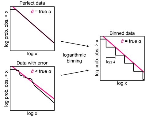
Figure 1: Cartoon overview. Logarithmic binning causes power law data with and without errors to converge toward the same discrete power-law distribution. Routine errors in data cause deviations from a perfect power law that bias estimates of the exponent $\hat{\alpha}$ and goodness-of-fit tests (bottom left). Logarithmic binning reduces the effect of error by smoothing data within each bin. After binning, data with errors better approximates perfect data from the discrete power law. Inference using the discrete power law then recovers unbiased estimates and stipulated false positive rates in goodness-of-fit tests.

We offer a novel method to tune the robustness of MLEs and K-S statistics to small errors without relying on specific information about the errors. Rather than model error explicitly, we reduce its affect by binning the input data as depicted in Fig. 1. Small errors by definition typically preserve the order of magnitude of each data point, and hence small errors and relatively large bins rarely allow data to move between bins, limiting the possible influence of errors. The power law, meanwhile, specifies frequencies across orders of magnitude, and so binning the data by order of magnitude preserves much of the useful information for inference.

Binning by orders of magnitude is a case of logarithmic binning, where the bin boundaries are integer powers of a ratio $\lambda>1$. Logarithmic binning and the power law distribution are both self-similar, and so power law samples also follow the power law with the original exponent after logarithmic binning (Newberry and Savage, 2019). The discrete distribution of the binned data has the same shape as the original, but ignores errors that are small relative to the binning ratio $\lambda$. Taking the limit of $\lambda\to 1^{+}$ recovers inference using the continuous Pareto distribution. The customary Pareto inference method is therefore an extreme case which is the most sensitive to error. The discrete power law thus provides a more robust general model for power-law distributed data, recovering the benefits of MLEs and K-S statistics even in the presence of small, unspecified errors.

We validate in simulation that logarithmic binning attenuates biases in estimates as well as restores specified false positive rates in goodness-of-fit tests on power-law data with noise. Furthermore these benefits can be achieved with a known and relatively small cost in increased statistical error on the estimator Efron and Hinkley (1978); Newberry and Savage (2019). We further find no impact on false negative rates in rejecting non-power-law data for some binning schemes, whereas others negotiate a tradeoff between false positive and false negative rates. These results show that logarithmic binning preserves most of the useful information for parameter estimation and hypothesis tests about power laws, while removing extraneous and misleading effects of noise.

We further show that observable errors in empirical datasets have caused biases in past inferences and incorrect conclusions about whether data originates from a power-law distribution. For example, errors such as rounding to the nearest tenth, on either a linear or logarithmic scale, can cause goodness-of-fit tests to reject data that otherwise fits the power law, whereas distributions with visually noticeable curvature across their entire range can be accepted as a power law unless binning induces the tests to adopt a broader perspective. We therefore conclude with the recommendation of logarithmic binning as a first step of inference in power law distributions.

2 Method

We propose logarithmic binning as a smoothing method to remove errors and reduce bias in parameter estimates and measures of goodness of fit. Given the minimum possible data value $x_{m}$, the logarithmic binning scheme is fully specified with a continuous parameter $\lambda>1$ specifying the ratio between adjacent bin boundaries. This bin width, $\lambda$, then controls the amount of smoothing. The limit $\lambda\to 1^{+}$ corresponds to no binning, since every unique data point occupies its own bin and the binned and unbinned data converge, whereas large $\lambda$ such as 2 or 10 bin the data by orders of magnitude and smooth out all information within each order.

Given input data $x_{i}$, we assign the binned value $\lfloor x_{i}\rfloor_{\lambda}=x_{m}\lambda^{k}$ where $k$ corresponds to the closest integer power of $\lambda$, rounding down. We denote binning using a floor operator with a subscript $\lambda$ because logarithmic binning is a floor operation in $\log_{\lambda}$ space: in terms of the usual integer floor, $\lfloor x\rfloor$, logarithmic binning is $\lfloor x\rfloor_{\lambda}=x_{m}\lambda^{\lfloor\log_{\lambda}x/x_{m}\rfloor}$.

We can derive an expression for the distribution of binned data. The possible values after binning are $x_{m}\lambda^{k}$ for $k=0,1,2,...$. By integrating the probability density function of the continuous power law (Eq. 2) over the range of each bin, the probability mass function for binned power-law data is given by

$$p_{d}(x_{m}\lambda^{k})=\int_{x_{m}\lambda^{k}}^{x_{m}\lambda^{k+1}}\mkern-25.0mup(x)\,dx=(1-\lambda^{-\alpha})(\lambda^{k})^{-\alpha}.$$ (3)

This discrete distribution is also a power law distribution since $\ln p_{d}=-\alpha\ln(x_{m}\lambda^{k})+c$, with exponent $\alpha$ equal to the $\alpha$ in Eq. 1. Logarithmic binning is the only binning scheme that preserves this property (Newberry and Savage, 2019). The continuous power law is scale-invariant, whereas the discrete power law (Eq. 3) has a discrete-scale invariance (Sornette, 1998) with the same scaling exponent.

For parameter estimation, we use the maximum likelihood estimator for the discrete distribution given by Newberry and Savage (2019),

$$\hat{\alpha}_{\lambda}=\log_{\lambda}\left[1+\left({1\over n}\sum_{i=1}^{n}\left(\log_{\lambda}\lfloor x_{i}\rfloor_{\lambda}-\log_{\lambda}x_{m}\right)\right)^{-1}\right],$$ (4)

using the logarithmically-binned data $\lfloor x_{i}\rfloor_{\lambda}$. This estimator is notably undefined for $\lambda=1$. However in the limit $\lambda\to 1^{+}$, $\hat{\alpha}_{\lambda}$ converges to the classical MLE for the Pareto distribution due to Muniruzzaman (1957), and so we call this estimator $\hat{\alpha}_{1}$,

$$\hat{\alpha}_{1}:=\lim_{\lambda\to 1^{+}}\hat{\alpha}_{\lambda}=\left({1\over n}\sum_{i=1}^{n}\left(\log x_{i}-\log x_{m}\right)\right)^{-1}.$$ (5)

Thus we index the estimator by the binning ratio $\lambda\geq 1$, with $\lambda=1$ representing the case of raw, unbinned data.

The variance of the MLE $\hat{\alpha}_{\lambda}$ is given by the inverse of the observed Fisher information (Efron and Hinkley, 1978; Virkar et al., 2014; Newberry and Savage, 2019) as

$$\sigma^{2}_{\hat{\alpha}_{\lambda}}=(\lambda^{\hat{\alpha}_{\lambda}}-1)^{2}/(n\lambda^{\hat{\alpha}_{\lambda}}\log^{2}\lambda).$$ (6)

This expression is also undefined for $\lambda=1$, but converges to $\sigma^{2}_{\hat{\alpha}_{1}}=\hat{\alpha}^{2}_{1}/n$ in the limit $\lambda\to 1^{+}$ and likewise corresponds to the variance on the Pareto MLE.

The variance on the estimator and hence the statistical error increase polynomially with $\lambda$ as $O(\lambda^{2\alpha})$. Conversely as $\lambda$ decreases, small errors are more likely to move data between bins and bias the estimator. Hence $\lambda$ negotiates a tradeoff between potential bias and statistical error, with some intermediate optimum that depends on the nature and severity of errors in the data. The Pareto MLE $\hat{\alpha}_{1}$ in common use occupies the extreme end of this spectrum with the least variance but also the greatest susceptibility to error.

As a goodness of fit measure, we use the Kolmogorov-Smirnov statistic $D$. The Kolmogorov-Smirnov statistic is the divergence between a sample and a reference distribution computed as the maximum difference between the empirical and null hypothesized cumulative distribution functions. For continuous distributions, the asymptotic distribution of $D$, the Kolmogorov distribution, is classically known exactly (Kolmogorov, 1933). The quantile of the $D$ computed from a sample provides a measure of goodness of fit to the distribution (Massey, 1951). Extreme quantiles, corresponding to low $p$-values, indicate discrepancies between the sample and the hypothesized distribution. The Kolmogorov-Smirnov test rejects the null hypothesis, in favor of the alternative hypothesis that the data originate from some other distribution, if the $p$-value is less than the stipulated false positive error rate. The $p$-value cutoff is equal to the stipulated false positive rate because if a sample truly originates from the reference distribution, the distribution of its quantile and $p$-value are uniform.

The Kolmogorov-Smirnov statistic for logarithmically-binned data $\lfloor x_{i}\rfloor_{\lambda}$ relative to the discrete power law (Eq. 3) is

$$D=\,\max_{k\in\{0,1,2,...,\infty\}}\left|{1\over n}\sum_{i=1}^{n}\mathbf{1}_{\lfloor x_{i}\rfloor_{\lambda}\leq x_{m}\lambda^{k}}-\sum_{i=0}^{k}p_{d}(x_{m}\lambda^{k})\right|,$$ (7)

where the sum over the indicator function $\mathbf{1}$ counts the number of data points in bins up to and including $x_{m}\lambda^{k}$. The resulting distribution of $D$, however, is not necessarily equal to the Kolmogorov distribution when the null hypothesized distribution is discrete or involves parameters estimated from the data (Noether, 1963; Walsh, 1963; Lilliefors, 1967). Therefore we build up an approximate distribution of $D$ under the null hypothesis by bootstrapping following Lilliefors (1967). We draw a sample of size $n$ from the discrete power law given by Eq. 3 with parameters $\lambda$ and $\hat{\alpha}_{\lambda}$, fit the parameter $\hat{\alpha}_{\lambda}^{\prime}$ to this sample, then compute $D$ for this sample using the parameters $\lambda$ and $\hat{\alpha}_{\lambda}^{\prime}$, thus simulating the steps for computing $D$ from the data. This procedure can be repeated on many samples from the discrete power law to build up an empirical distribution of $D$ that successively better approximations to the true null distribution. The $p$-value is one minus the quantile of $D$ computed from the data among the samples of $D$ computed through bootstrapping. This goodness-of-fit test follows a popular method (Clauset, Shalizi and Newman, 2009; Gillespie, 2015) that has also been adapted to binned power-law data (Virkar et al., 2014). Our test differs only in that we do not jointly estimate $x_{m}$, as our analysis fixes $x_{m}=1$. In lieu of computing precise $p$-values by bootstrapping many samples, we just as accurately judge whether $p<0.05$ using only 19 bootstrapped values, concluding that $p<0.05$ if the $D$ observed in the data exceeds all 19.

This logarithmic binning method allows the experimenter to specify $\lambda$ based on tolerances of bias and statistical error. The magnitude of bias cannot be estimated directly for unknown sources of error. We provide tolerances (see Validation) for the case of additive and multiplicative normal noise. In principle, bias can be minimized by choosing $\lambda$ to exceed relative error on the vast majority of data points or to choose $\lambda$ as high as possible. Upper limits for $\lambda$ depend on the application. A given tolerance for statistical error imposes an upper limit on $\lambda$ given by Eq. 6. Even with unlimited tolerance for statistical error, data must occupy at least two bins for $\hat{\alpha}_{\lambda}$ to be defined. The number of bins is equal to $\lfloor\log_{\lambda}\max_{i}x_{i}/x_{m}\rfloor+1$. Hence the maximum feasible $\lambda$ is equal to the proportional range of the data, $r:=\max_{i}x_{i}/x_{m}$. The corresponding $\hat{\alpha}_{r}$ minimizes bias but also has the highest possible statistical error and is useless for foreseeable practical applications. Hypothesis testing imposes more restrictive upper limits on $\lambda$. Generally, $\lambda$ should be constrained by the capacity to reject alternative distributions. What values this constraint imposes unfortunately depends on the alternative distribution, which is often unspecified. One extreme upper limit is given by requiring at least three bins. With data in only two bins, $\hat{\alpha}_{\lambda}$ can be typically be chosen to fit the data exactly so that $D<1/n$ in every bootstrap sample. The probability a bootstrap run contains fewer than three bins is given by the formula

$$\Pr(\max_{i}x_{i}<\lambda^{2})=\left(1-\left(\lambda^{2}\over x_{m}\right)^{-\alpha}\right)^{n}$$ (8)

derived from Eq. 1. Setting this expression equal to the tolerable fraction of bootstrap simulations with fewer than three bins gives the theoretical upper limit on $\lambda$. In practice, other considerations such as false negatives rates will further restrict the upper limit of $\lambda$ for purposes of hypothesis testing.

3 Validation

We validate the performance of binning by synthesizing pure continuous power-law samples and introducing normal additive and multiplicative (proportional) noise. We generate parameter estimates and goodness of fit measures for different levels of binning from no binning to the extremes allowed by the data. We compare the known, true parameters to the estimated parameters and compare the sensitivity and specificity of goodness-of-fit tests with and without binning.

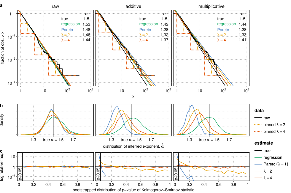
Figure 2: Error in power-law data biases estimates of the exponent $\alpha$ and causes tests based on Kolmogorov-Smirnov (K-S) statistics to reject the power-law distribution. (a) Log-log tail distribution plots of samples from perfect data (left) and data with additive and multiplicative noise are visually almost indistinguishable (middle: Normal(0, $\sigma_{+}^{2}$=0.2), right: Lognormal(0, $\sigma_{\times}^{2}$=0.2)). This noise nonetheless biases estimates of the log-log slope $-\alpha$ relative to the true $\alpha$=1.5. Logarithmic binning with $\lambda$=2 or $\lambda$=4 (dotted lines) brings the slope estimates $\hat{\alpha}_{\lambda}$ closer to the true value. (b) Distributions of the slope estimates over 1000 samples of size $n=500$ illustrate a tradeoff between accuracy and precision, where the most precise estimation methods are also the most inaccurate. (c) Distributions of $p$-values for rejecting the power law based on a K-S statistic are uniform when the data comes from a perfect power law, with or without binning (left). However, noise biases $p$-values (middle, right) so that the K-S statistic that assumes a continuous power law (blue) has $p$¡0.05 more than 50% of the time. Binning with $\lambda$=2 or $\lambda$=4 attenuates noise, brings $p$-value distributions closer to uniformity, and restores stipulated false positive rates.

We synthesize data by drawing $n$ independent samples $x_{i}$ from a Pareto distribution (Eqs. 1, 2) with parameters $\alpha$ and $x_{m}$. Without loss of generality, we set $x_{m}$ to 1, since the general case can always be mapped to $x_{m}=1$ by converting the units of $x$. We simulate experimental error using either unbiased additive (normal) or multiplicative (lognormal) noise with variance $\sigma_{+}^{2}$ and $\sigma_{\times}^{2}$ respectively. The data with additive noise is constructed from a sample $x_{i}$ as $x_{i}+\operatorname{Normal}(0,\sigma_{+})$ and multiplicative noise as $x_{i}\times\operatorname{Lognormal}(0,\sigma_{\times})$. For $x_{m}\neq 1$, the corresponding additive variance is $x_{m}\sigma_{+}$, since $\sigma_{+}$ has the same units as $x$, whereas the corresponding multiplicative variance is still $\sigma_{\times}$ since $\sigma_{\times}$ is a dimensionless log-ratio. Fig. 2a shows tail distribution plots of samples generated with each kind of noise.

As a proof of principle, we take 1000 samples of size $n=500$ and $\alpha=1.5$ with and without additive and multiplicative noise with $\sigma_{+}=\sigma_{\times}=0.2$ in order to generate empirical distributions of estimates $\hat{\alpha}$ and bootstrapped $p$-values of the K-S statistic (Fig. 2). For each sample we estimate $\alpha$ and compute the $p$-value both without binning (Pareto) and using logarithmic binning with $\lambda=2$ and $\lambda=4$. We additionally estimate $\alpha$ as the slope by ordinary least squares regression on the empirical cumulative distribution function—the log of each data point versus the log of its quantile in the sample, for which no binning is necessary.

Fig. 2 shows how much the errors can bias estimates of $\alpha$ and $p$-values. All estimates and $p$-value behave as expected in samples without error: the estimates cluster around the true value and distributions of $p$-values are uniform regardless of $\lambda$. The averages of each MLE $\hat{\alpha}_{\lambda}$ are within 0.21% of the true value whereas the average regression estimate is within 1.2%. In samples with noise however, the naïve Pareto MLE $\hat{\alpha}_{1}$ is biased by around 10%, confidence intervals on $\hat{\alpha}_{1}$ typically exclude the true value, and $p$-values approach zero. This observation parallels empirical findings that errors in the data such as measurement error or quantization noise can substantially bias MLEs in practice (Langlois, Cousineau and Thivierge, 2014; Newberry and Savage, 2019).

Coarser binning, with larger values of $\lambda$, brings the MLEs $\hat{\alpha}_{\lambda}$ closer to the true value on average and brings the distribution of $p$-values closer to uniform. In all noise treatments, binning with $\lambda=4$ yields approximately uniform $p$-values and regression provides approximately unbiased estimates of $\alpha$.

Bias and variability of estimates of $\alpha$ illustrate a clear tradeoff between accuracy and precision. As expected for maximum likelihood estimation, $\hat{\alpha}_{1}$ is the most efficient and the distribution of $\hat{\alpha}_{1}$ is the most sharply peaked (Fig. 2b). However, $\hat{\alpha}_{1}$ is correspondingly the most sensitive to errors in the data and thereby produces the most biased estimates. Binning makes the $\hat{\alpha}_{\lambda}$ progressively less sensitive to error for $\lambda=2$ and $\lambda=4$, while providing more precise estimates than linear regression. Estimates by linear regression are the most accurate as well as the most variable. On the whole, linear regression minimizes the squared difference between the estimates and the true value in this example, despite its lack of theoretical guarantees.

Noise also causes the bootstrapped K-S $p$-values to reject the Pareto distribution nearly all of the time (additive: 97% multiplicative: 93%), in contrast to a stipulated false positive rate of 5% (Fig. 2c). In one sense, the test is correctly performing its job: the null hypothesis specifies that the sample originates from the Pareto distribution, whereas the distribution of the sample is Pareto convolved with noise. By a strict interpretation, the null hypothesis is correctly rejected. In a more practical sense however, the data comes from a power law whether or not small errors are invovled, and so rejecting the power law is incorrect and constitutes a false positive. All measurements have errors, and so in this sense, which we adopt here, errors in the data obscure the truth by causing extreme bias in the $p$-values.

Binning the data brings $p$-values back to an approximately uniform distribution, as shown in Fig. 2c. Binning blinds the test to differences in the shape of the empirical and hypothesized distributions within each scale—including differences due to discretization and measurement errors—while still accounting for the shape of the distribution across the range of the data. With $\lambda=2$, the false positive rates fall to 23% and 34% on data with additive and multiplicative noise, respectively. With $\lambda=4$, the rejection rates in these 1000 trials are consistent with the stipulated rejection rate of 5% at 5.4% and 6.1% respectively. More trials would reveal biases on the order of 1%, but these K-S $p$-values are valid for purposes of roughly controlling the false positives rate. That is, after binning by sufficiently large $\lambda$, data originating from a power law, errors or not, will be rejected as a power law with $p<0.05$ roughly 5% of the time.

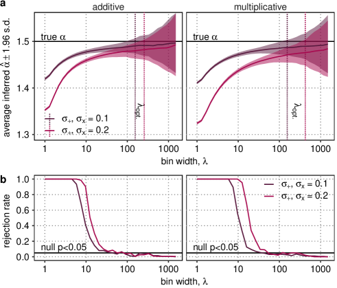
Figure 3: The binning ratio $\lambda$ tunes (a) a tradeoff between accuracy and precision of the estimator $\hat{\alpha}_{\lambda}$ and (b) robustness of hypothesis tests, on data with additive and multiplicative noise. Here we simulate large datasets ($n$=1,000,000, median range $r$=14,267, 200 replicates) with additive and multiplicative noise with variance $\sigma_{+}$ and $\sigma_{\times}$ = 0.1 and 0.2. (a) Increasing $\lambda$ brings estimates $\hat{\alpha}_{\lambda}$ closer to the true $\alpha$=1.5 but also increases the variance of the estimator. The optimal binning ratio $\lambda_{\mathrm{opt.}}$ to minimize total mean squared error on the estimate depends on the type and magnitude of noise but roughly divides the data into two bins. (b) Hypothesis tests virtually always reject the power law unless $\lambda$ is sufficiently large relative to noise. Rejection rates roughly equal the stipulated $p$-value cutoff 0.05 when $\lambda\approx 70$ in all noise treatments whereas yet greater values of $\lambda$ produce conservatively biased $p$-values. The range of $\lambda$ that achieves the stipulated false positive rate corresponds to dividing the data into 3-4 bins.

The binning ratio $\lambda$ controls the tradeoff between accuracy and precision in estimates and the robustness of hypothesis tests to noise, as shown in Fig. 3. Increasing $\lambda$ attenuates noise but also removes information from the sample. Biases in $\hat{\alpha}_{\lambda}$ therefore decrease with $\lambda$ whereas variability of the estimator (Eq. 6) increases. We empirically investigated this tradeoff on large samples by fitting $\hat{\alpha}_{\lambda}$ and conducting hypothesis tests across a range of $\lambda$ (200 replicates; $n$=1,000,000; $\alpha=1.5$; $\sigma_{+},\sigma_{\times}=0.1,0.2$). For each noise treatement we found a $\lambda_{\mathrm{opt.}}$ that minimized the total mean squared error on the estimator, $(\alpha-\hat{\alpha}_{\lambda})^{2}$, incorporating both bias and variability. This $\lambda_{\mathrm{opt.}}$ typically divided the data into two bins. Specifically, setting $\log\lambda/\log r=0.50$ with $r=\max_{i}x_{i}/x_{m}$ equally divides the range of the data in log space (median: $r$ = 14,267, $\lambda_{0.50}=119$). We observed $\log\lambda_{\mathrm{opt.}}/\log r$ ranging from 0.49 to 0.63 across all noise treatments. Doubling the noise leads to only marginally larger $\log\lambda_{\mathrm{opt.}}/\log r$, suggesting that equally dividing the range of the data into two bins is a reasonable generic prescription for minimizing bias and variability when detailed information about errors in the data is not available.

Binning with sufficiently large $\lambda$ restored stipulated false positive rates in hypothesis tests (Fig. 3b). On these large samples, the hypothesis test nearly always rejects the power law unless $\lambda$ is also large. The minimum $\lambda$ to achieve the stipulated false positive rates depends on the type and magnitude of noise and ranged from $\lambda=20$ to $\lambda=60$. For yet higher $\lambda$, $p$-values become conservatively biased from too few bins (see Methods), causing fewer than the stipulated rate of false positives. In all four treatments, $\lambda$ in the range from 60 to 75 gave rejection rates that were not significantly biased upwards or downwards from the stipulated rate of 0.05 over 200 trials (one-tailed binomial $p$-values: 0.12 to 0.87). According to Eq. 8, the bias from too few bins at $\lambda=75$ is less than 10% or 0.005 while the bias due to errors in the data is minimized. Thus robust $p$-values are available for $\lambda=75$ across all treatments as well as for lower $\lambda$ in treatments with lower error.

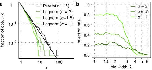
Figure 4: For (a) lognormal samples chosen to resemble the power-law, (b) binning entails no decrease in statistical power below a threshold of $\lambda$. (a) Samples ($n$=500) from the tail of the lognormal distribution can approximate power-law samples arbitrarily well by increasing the lognormal variance $\sigma$. (b) The statistical power (rejection rate) on these samples is unaffected by binning provided $\lambda<2$, corresponding to dividing the data into at least four bins.

Statistical power or sensitivity is the test’s ability to correctly reject non-power-law data. Intuitively sensitivity might decrease with $\lambda$ since binning removes information. We investigate how binning affects the ability to reject non-power-law data by applying the test to small samples ($n=500$) from the tail of the lognormal distribution truncated below $x_{m}=1$. The lognormal distribution, like the power law, is heavy-tailed and so its extremes can be difficult to distinguish from a power law. Both tail distributions can appear straight on a log-log plot, but the lognormal has curvature that depends on its parameters (Fig. 4a). The truncated lognormal distribution has three parameters, the mean and variance $\mu$ and $\sigma$ as well as the tail threshold $x_{m}$ that samples must exceed. The slope and curvature of the lognormal tail depend on all three parameters. We set $x_{m}$ to 1, use $\sigma$ to set the curvature, and finally choose $\mu$ so that the log-log slope of the lognormal tail distribution at $x_{m}$ is equal to a power law with $\alpha=1.5$. In this scheme, the lognormal tail can approximate the power law arbitrarily well as the lognormal variance $\sigma$ increases.

For samples from the lognormal tail, we find that the test sensitivity is unaffected by binning, provided $\lambda$ divides the data into at least four bins (Fig. 4b). The test’s rejection rate on lognormal data depends strongly on the curvature of the lognormal distribution and the amount of data. For $\sigma=1$, the test rejects lognormal data roughly 80% of the time regardless of $\lambda$ for all $\lambda<2$. The median range of these samples is 12.8, and so $\lambda=2$ typically puts the maximum data point in the fourth bin, [8,16). As $\sigma$ increases, so too does the maximum value in samples, which widens the range of $\lambda$ that divide the data into four bins. One quick, intuitive rationalization for the significance of four bins is that only three points are required to detect curvature, while the topmost bin is unreliable and only partially occupied by the range of the data.

Chosing $\lambda$ within a certain range tunes a tradeoff between sensitivity and specificity. Our earlier measurements in noisy power-law samples of the same size ($n$=500, Fig. 2) give the specificity. While the sensitivity is the rate of rejection on lognormal tail samples, the specificity is the rate of acceptance on noisy power-law samples or one minus the false positive rate. The test with $\lambda=2$ and a $p$-value cutoff of 0.05 distinguishes lognormal tail samples with $\sigma=1$ from noisy power-law samples with a sensitivity of 78% and specificities of 77% for additive noise and 66% for multiplicative with $\sigma_{+},\sigma_{\times}=0.2$. Using $\lambda<2$ yields reduced specificity with no benefit to sensitivity, whereas $\lambda>2$ tunes a tradeoff between sensitivity and specificity. Using $\lambda=3$ for example gives sensitivity of 37% and specificities of 92% and 89% on the same samples. For $\lambda>4$ sensitivity approaches zero and the test is useless. The interval $2<\lambda<4$ then offers reasonable tradeoffs between sensitivity and specificity, with lower $\lambda$ more sensitive and higher $\lambda$ more specific.

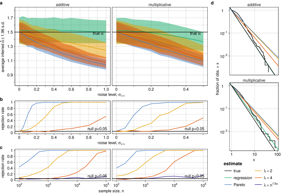
Figure 5: Increasing noise $\sigma_{+}$ and $\sigma_{\times}$ (a) increases bias in estimates of $\alpha$ as well as (b) the rate of rejecting the power-law distribution in samples of size $n=500$, while (c) increasing sample size $n$ increases the rejection rate without affecting bias in $\hat{\alpha}_{\lambda}$ in samples with $\sigma_{+},\sigma_{\times}=0.2$. At the upper limit of the plotted range, where $\sigma_{+}=1.0$ and $\sigma_{\times}=0.5$, (d) the tail distributions of samples are notably curved and no longer resemble a power law on log-log plots, producing extremely biased estimates of the slope. Binning with $\lambda=2$ or 4 (yellow, red) reduces bias in estimates and restores rejection rates to the stipulated 0.05 over a larger range of tolerable error.

The foregoing results demonstrate cases in which binning has the desired effect of reducing the influence of small errors in the data at modest cost of statistical power. The qualitative results hold more generally, while exact magnitudes of bias and rejection rates depend on the errors, the sample size, and $\alpha$. The test sensitivity and how it depends on $\lambda$, on the other hand, depend on the possible alternative distributions, which we cannot enumerate explicitly.

We can quantitatively generalize the results by varying $\sigma$ and sample size $n$. Biases in $\alpha$ increase with greater error magnitudes and decrease with greater $\lambda$, while false positive rates as well as the feasible values of $\lambda$ depend strongly on sample size (Fig. 5). We choose a range of errors from 0 (no error) to a maximum error high enough that the distribution clearly deviates from a straight line on a log-log plot and no one slope clearly represents the distribution (Fig. 5b). The error rates $\sigma_{+}$ and $\sigma_{\times}$ each have marginal effects on biases in $\alpha$ (Fig. 5a), whereas the biases do not depend on $n$ because greater sample size merely causes the estimators to converge to their expected values. Precision of the estimates, by contrast, increases with sample size, as expected from Eq. 6. This feature can be problematic because as sample size increases, estimators are more confident in an incorrect estimate and confidence intervals are more likely to exclude the true value. Fortunately increasing $n$ also increases the feasible range of $\lambda$ and the maximum $\lambda$ subject to a tolerable statistical error. Hence increasing sample size can mitigate bias by concommittantly increasing $\lambda$ according to Eq. 6.

Rejection rates exhibit sigmoid threshold behavior in both $\sigma$ and $n$ similar but opposite to the thresholds in $\lambda$ (Fig. 5c, Fig. 3). For sufficiently small error or sample size, the test cannot detect errors, $p$-value distributions are close uniform, and hence rejection rates are equal to the $p$-value cutoff such as 0.05. As error or sample size increases, hypothesis tests are more likely to detect the errors and reject the power law until eventually the errors or sample size are sufficient for the test to nearly always reject. Increasing $\lambda$ increases the threshold of $\sigma$ or $n$ at which the test begins to detect errors and reject the power law. With $\lambda=1$ (no binning) there is almost no range of tolerable error. For example, noise with $\sigma_{+}=0.025$ roughly doubles the false positive rate. For $\lambda=4$, on the other hand the noise must exceed $\sigma_{+}\geq 0.4$ or $\sigma_{\times}\geq 0.3$ before the rejection rate is doubled. While noise can easily be increased to the point that no feasible binning is sufficient to restore the stipulated rejection rates, increasing $n$ allows greater $\lambda$ by increasing the range of the data. In Fig. 5, we set $\lambda$ to $n^{1/(3\alpha)}$ (purple), designed to typically bin the data into 3 or 4 bins. Allowing this $\lambda$ to depend on $n$ preserves approximately unbiased $p$-values over the range of $n$ from 100 to 100,000.

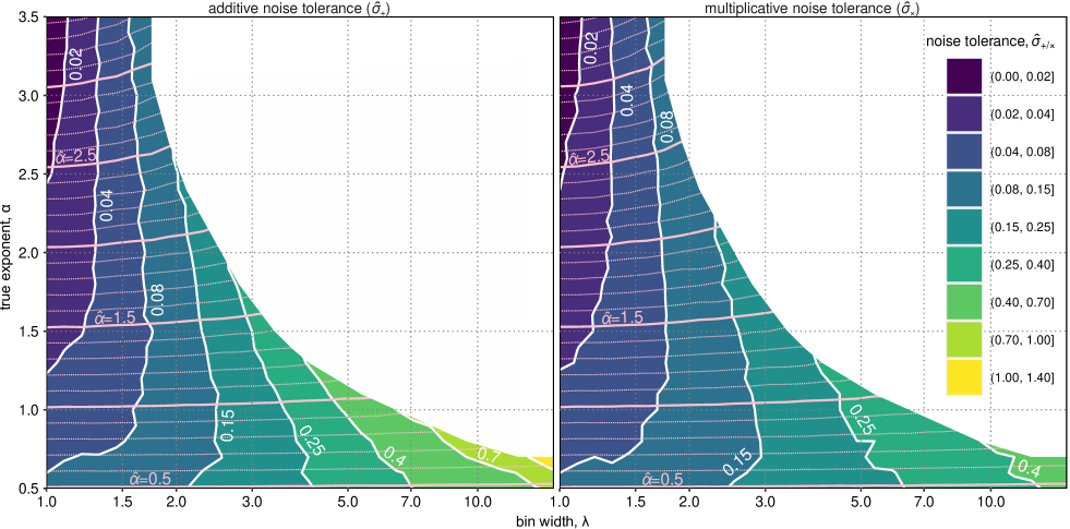
Figure 6: The noise tolerance for a given $\alpha$ and $\lambda$ is the level of noise $\sigma_{+}$ or $\sigma_{\times}$ at which bootstrapped K-S $p$-values are less than 0.05 roughly 10% of the time. Shown here are noise tolerance contours for samples of size $n$=500. With this amount of error, $p$-values are biased enough to double the false positive rate relative to the stipulated rate of 0.05. More error quickly renders hypothesis tests meaningless, while less error, greater $\lambda$, or lower $n$ can restore the actual false positive rates closer to the stipulated 5%. The inferred $\hat{\alpha}_{\lambda}$ (pink contour lines) are also biased to some degree by this amount of noise, as they differ from the horizontal lines of true $\alpha$. Bias in $\hat{\alpha}_{\lambda}$ increases with $\sigma_{+/\times}$ but decreases with $\lambda$ so that as $\sigma_{+/\times}$ increases with $\lambda$, the contour lines remain roughly horizontal and bias remains within 10% of the true $\alpha$.

The parameter $\alpha$ also influences the error threshold and magnitudes of bias in the MLEs. We varied $\alpha$ and $\lambda$ over a grid of combinations and computed error thresholds as the $\sigma_{+}$ or $\sigma_{\times}$ required to double the rejection rate for a $p$-value cutoff of 0.05. For each $\alpha$ we varied $\lambda$ from 1 to $n^{1/3\alpha}$, which at its maximum still divided the data into at least four bins at least 70% of the time. We conducted a stochastic binary search to estimate these values $\hat{\sigma}_{+}$ and $\hat{\sigma}_{\times}$, testing various candidate $\sigma$-values and concluding the search when the target rejection rate 0.10 was within a binomial 95% confidence interval of $\pm 0.005$ for trials in the interval $\hat{\sigma}\pm 0.02\hat{\sigma}$. This search thus yields values $\hat{\sigma}$ which are within 2% of some $\sigma$ for which the rejection rate is within 5% of 0.10 approximately 95% of the time. The search also yields mean estimates $\hat{\alpha}_{\lambda}$ at the inferred noise level.

Fig. 6 thereby gives an error tolerance for hypothesis tests and the maximum bias on estimates within that error tolerance applicable to samples of $n=500$. For example, at the values $\alpha=1.5$ and $\lambda=2$, additive noise with $\sigma_{+}<0.08$ gives a rejection rate less than 0.1 and $\hat{\alpha}_{\lambda}$ slightly less than 1.5, biased by approximately 0.05 corresponding to results presented in Fig. 5. The lines of inferred $\hat{\alpha}_{\lambda}$ are approximately horizontal and approximately equal to $\alpha$ because limiting noise to levels that do not substantially affect hypothesis tests also limits noise that would substantially bias $\hat{\alpha}$. At the maximum such $\hat{\sigma}_{+}$ or $\hat{\sigma}_{\times}$ for any given $\alpha$, the magnitude of bias $\hat{\alpha}-\alpha$ is still less than 10% of $\alpha$ when binning by the corresponding $\lambda$.

Conversely, for a known amount of noise, Fig. 6 gives a lower bound for $\lambda$ at a given inferred $\alpha$. For example, on data with a known $\sim$10% proportional random noise, $\sigma_{\times}\approx 0.1$ and hence, if inferred $\alpha=1.5$, $\lambda$ should be chosen to exceed roughly 2.2 in order to remain within a 10% tolerance of bias on $\alpha$ and a less-than-doubled false positives rate. Normal additive and multiplicative noise can be taken as a proxy for many kinds of measurement errors that routinely occur in data, and so Fig. 6 provides lower bounds on valid $\lambda$ for a variety of error types in samples of size $n=500$.

4 Results

We analyse three empirical cases and compare results with and without binning. We use data on earthquake magnitudes and wealth, which are historically believed to follow power-law distributions, as well as wildfire size, for which we have no evidence of a power law. The specific datasets are curated online by Clauset, Shalizi and Newman (2009) as demonstration cases of power-law inference. The earthquakes dataset contains 17,450 positive and valid samples, recorded as two-digit Richter magnitudes ranging from 0.5 to 7.8. The Richter scale records the logarithm to the base 10 of the amplitude of waves recorded by seismographs (Richter, 1935). We convert the data back to the natural scale by exponentiating the Richter magnitudes. The result is a dataset with discrete values proportional to integer powers of $\lambda=10^{0.1}\approx 1.26$. In other words, Richter magnitudes with two digits of precision are inherently a case of logarithmic binning with $\lambda=10^{0.1}$. The wealth dataset is the Forbes list of the world’s 399 richest people in 2003, including 261 billionaires. The wildfires dataset includes 203,784 measurements of wildfire area from one decade in the US, 99% of which are between $10^{-1}$ and $10^{3}$ acres.

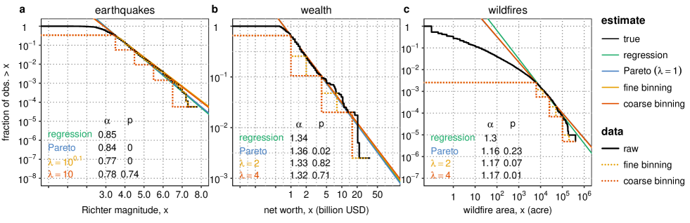
Figure 7: Binning reverses conclusions about whether (a) earthquake magnitudes, (b) wealth, and (c) wildfire area follow a power law distribution. Measurement or recording errors and quantization noise (a,b) bias MLEs and invalidate goodness-of-fit tests whereas binning the data attenuates the influence of errors and induces more reasonable conclusions. For data that does not follow a power law (c), binning correctly rejects the power law when the test would otherwise accept it.

We estimate the exponent $\alpha$ and conduct goodness-of-fit tests for all three datasets using the MLEs $\hat{\alpha}_{1}$ and $\hat{\alpha}_{\lambda}$ and K-S statistics just as with the synthetic data. For each dataset we compare three binning treatments—no binning ($\lambda=1$), fine binning (small $\lambda$) and coarse binning (large $\lambda$)—letting the small and large $\lambda$ depend on the dataset. We also estimate the exponent with linear regression against the empirical cumulative distribution function as with the synthetic data in Fig. 2. We stipulate a fixed $x_{m}$ for each dataset, specifically, magnitude 3.5 for earthquakes, one billion dollars for wealth, and 6324 acres for wildfires.

The earthquake dataset incorporates errors known to complicate measurements, including partial censorship of small values, quantization error, and attraction to particular values. Fig. 7a demonstrates that these subtle errors have different effects on MLEs and goodness-of-fit tests at different $\lambda$. We avoid the partial censorship that causes visible curvature in Fig. 7a by choosing $x_{m}=10^{3.5}$, or magnitude 3.5, across all treatments. This minimum magnitude without censorship is called the magnitude of completeness or $m_{c}$ in seismology (Woessner and Wiemer, 2005) and depends on the density of the earthquake sensor network. The earthquake dataset also includes quantization error from the two-digit precision of Richter magnitudes. This quantization error is equivalent to logarithmic binning, and so we choose the fine bin width as $\lambda=10^{0.1}$ to exactly match the quantization in the raw data. This “binning” preserves the input data exactly but entails a different estimator, $\hat{\alpha}_{10^{0.1}}$, and a different bootstrapped distribution of K-S statistics. Hence the fine-binned ($\lambda=10^{0.1}$) and unbinned ($\lambda=1$) empirical cumulative distributions in Fig. 7a overlap perfectly. The effect of quantization error per se is then evident from the difference between the Pareto MLE $\hat{\alpha}_{1}=0.84$, which assumes no quantization, and the appropriate MLE for the raw data, $\hat{\alpha}_{10^{0.1}}=0.77$. These values differ by 0.07 or 9%, comparable to the 12% magnitude of bias due to quantization error in a different earthquake dataset (Newberry and Savage, 2019).

We also observe abnormalities in the earthquake dataset at special magnitudes 3.0, 3.5, 4.0, 4.5, etc., each of which contains markedly more observations than adjacent magnitudes. The effect is highly statistically significant ($p<0.0001$, 1 d.f. $\chi^{2}$ test for association between multiples of 0.5 and higher-than-previous values) and easily explained if the dataset combines low-precision data quantized by 0.5 with high-precision data quantized to 0.1. Binning using coarse bins with $\lambda=10$ corresponding to a difference of 1.0 in Richter magnitude completely removes this artifact. Coarse and fine binning provide consistent estimates $\hat{\alpha}_{10^{0.1}}\approx\hat{\alpha}_{10}=0.78$ even with wildly different bin widths, but come to opposite conclusions in goodness-of-fit tests: $p$=0.76 with $\lambda=10$ whereas otherwise $p$¡0.01. Indeed, with no binning or fine binning by $\lambda=10^{0.1}$, the artifact persists. This data is inconsistent with a power law simply because more observations occur at increments of 0.5 than could be explained by chance. With $\lambda=10$, however, the artifact is removed and we conclude that the earthquake data is consistent with a power law. This binning still divides $n$=5,910 observations into 5 bins—offering plenty of capacity to reject alternative distributions relative to our simulations in which $n$=500 and 4 bins were sufficient to reject lognormal data. We therefore conclude that despite its flaws, the data provide strong evidence that the underlying phenomenon of earthquake magnitudes is consistent with power-law scaling across earthquake magnitudes 3.5 to 7.8, in agreement with geological studies and conventional wisdom.

The wealth dataset contains artifacts due to discretization on a linear scale, as well as known and unknown limitations on accurate measurements of the wealth of the extremely rich (Piketty, 2014). We choose $x_{m}=10^{9}$—one billion US dollars—for the Forbes list’s celebrated reputation for tracking the wealth of billionaires. This dataset includes striking discrepancies in its quantification scheme, with values truncated to the nearest 5 million or 100 million depending on whether net worth exceeded one billion, evident in different levels of jaggedness below and above 1 in the curve of Fig. 7b. The log-log plot also suggests inconsistent representation of values between 4 billion and 10 billion, where many billionares are represented has having either “4,000,000” or “5,000,000” while others are distinguished between 9.7 and 9.8 billion, particularly if net worth is just shy of a round number, resulting in noticeable “bumps” in the tail distribution. In this dataset, all three MLEs and regression obtain similar $\alpha$ estimates, but goodness-of-fit tests with and without binning draw distinct conclusions. As we observe in the earthquakes data, quantization noise can be sufficient for K-S $p$-values bootstrapped from the continuous Pareto distribution to reject the power law. Without binning, the MLE $\hat{\alpha}_{1}$ produces a slope aligned with a majority of data points in the dataset and consistent with the other estimates, but the K-S statistic rejects the hypothesis that wealth is drawn from a power-law distribution with $p=0.03$. Binning by either $\lambda=2$ or $\lambda=4$ attenuates the impact of bumps on the goodness-of-fit test, which then consistently accepts the power law, vindicating Vilfredo Pareto’s 1895 assertion.

The wildfire data represents a contrasting case with ample data recorded consistenly at $\pm$0.1 acre with up to six digits of precision. A basic visual inspection of the distribution in Fig. 7c reveals smooth and substantial curvature clearly inconsistent with a power law, even allowing for random variation. Methods for fitting $x_{m}$, however, have been devised to locate subsets of the distribution which do follow a power law. Clauset, Shalizi and Newman (2009) found power-law behavior above $x_{m}=6324$ using K-S statistics fitting both $x_{m}$ and $\alpha$. The remaining 520 values eliminate 99.7% of the data, indicating that the large proportion of data does not follow a power law indeed. Given $x_{m}=6324$ however, MLEs are consistent regardless of binning whereas the regression estimate differs, possibly indicating curvature persisting beyond 6324. The $p$-values with and without binning, however, are poles apart. The goodness of fit test to the continuous Pareto distribution accepts the null hypothesis with $p=0.26$, consistent with the stipulation for choosing $x_{m}$ initially. Tuning the bin width, $\lambda$, however, drives the goodness-of-fit test towards rejecting the power law. For $\lambda=4$, corresponding to four bins with only one data point in the fourth bin, we reject the power law with $p=0.01$. As we see in the other empirical cases, K-S statistics for continuous data ascribes undue weight to smoothness of the data, whereas in the present case binning conversely causes the K-S test to ascribe more weight to the overall shape of the distribution. The result is that binning allows the K-S statistics to reveal curvature in the empirical distribution when they otherwise do not.

5 Discussion

On perfect power-law data, estimates and goodness-of-fit tests give consistent results with and without binning, and binning can only reduce statistical power (Virkar et al., 2014). When the data deviates from a perfect power law, however, binning may reduce biases in inferences. Logarithmic binning preserves a power law with the original exponent, and so we argue that the resulting discrete power law (Newberry and Savage, 2019) is a better baseline model for real data than the Pareto distribution. When conclusions depend on binning, as we observe in the empirical data, the data deviate from a perfect power law, possibly for trivial reasons such as small errors. In this case, inferences without binning cannot be trusted, as the deviations bias the inference, and inferences based on binned data are more robust.

We find that logarithmic binning can attenuate the affects of additive and multiplicative noise and linear and logarithmic quantization errors. Real data contains many more sources of error, such as censorship or reporting biases, various kinds of measurement error, or dependence between samples. The argument for logarithmic binning makes no reference to the exact structure of the errors so long as the errors do not tend to cause the average addition or removal of data from particular bins. This requirement is much less stringent than requiring samples to be within statistical deviation of the perfect continuous power law. For errors such as noise and quantization that have small effects on individual measurements, the requirements can be assured if the binning ratio $\lambda$ is sufficiently large relative to the scale of the error. How large is sufficient depends on the purpose of the inference and the size of the sample (Figs. 3, 5, and 6).

Loose specification of errors is convenient in practice, because the details of error sources are often unknown. Nonetheless, we expect that binning is effective in attenuating some error types more than others. Binning may be less effective against errors that cause deviation from the pure power law over its full range, such as scale-dependent censorship (Woessner and Wiemer, 2005), contamination, or dependence between samples (Gerlach and Altmann, 2019). These cases need further investigation, but our study nonetheless offers some clues.

Model misspecification near $x_{m}$ and log-periodic fluctuations are two common causes of deviation from pure power laws. We do not study these cases explicitly, but our results do have bearing. Often, values near $x_{m}$ do not follow a perfect power law and log-log tail distribution plots show substantial curvature in small values. Small values may be censored, as in earthquake reporting, or may represent a bulk distribution with distinct behavior from the tail. Despite dealing only with small measurement noise, our validation procedure is nonetheless a reasonable proxy for both cases. Because we simulate noise by sampling from a power law above $x_{m}$, applying error, and then, of necessity, fitting using only the data above $x_{m}$, the procedure acts both to create a censorship process—because data reduced below $x_{m}$ by noise are removed from the sample—and a bulk distribution distinct from its tail—because applying normal or lognormal error to power law samples yields a unimodal distribution peaked near $x_{m}$. Thus samples with higher error such as those in Fig. 5 show more of the notorious curvature for small values common in empirical data. In such cases, increasing $x_{m}$ is known to reduce biases (Danielsson et al., 2001). Our results show that increasing $\lambda$ also reduces bias from this type of error, offering an alternative or additional measure of conservatism besides increasing $x_{m}$.

Log-periodic fluctuations are another deviation from power-law behavior common in empirical data. This phenomenon can result from dependence between data points in the sample, such as large blood vessels branching into smaller vessels (Newberry, Ennis and Savage, 2015) or large social groups composed of proportionally smaller units (Zhou et al., 2005). While Pareto samples display a continuous scale invariance, data with log-periodic fluctuations has a discrete-scale invariance, with a fundamental scaling ratio $\lambda$ set by the “wavelength” of the fluctuations (Sornette, 1998). If the bin width $\lambda$ matches the scaling ratio $\lambda$, the discrete-scale invariance of the model matches that of the data, conformity to the discrete power law is restored and inferences will be valid (Newberry and Savage, 2019). Thus, we expect data with log-periodic fluctuations may be accurately fit with logarithmic binning as long as care is taken to choose bin widths $\lambda$ that are integer powers of the fundamental scaling ratio of the data.

Our findings challenge some conventional wisdom about power law inference while addressing some ongoing concerns. Maximum likelihood estimation offers strong mathematical guarantees whereas regression has a manifestly incorrect error model (Goldstein, Morris and Yen, 2004; Bauke, 2007; Clauset, Shalizi and Newman, 2009; Stumpf and Porter, 2012). At the same time, the fragility of maximum likelihood in the case of power laws has been underappreciated, and we find that appropriate regression methods are relatively robust in practice (cf. Fig. 2, Gabaix and Ibragimov (2011)). Logarithmic binning offers MLEs the robustness of regression while maintaining the logical footings of maximum likelihood. The parameter $\lambda$ offers a smooth interpolation between the ideal precision of the continuous MLE and the accuracy of a vague and broadly-applicable error model.

Considerable discussion in recent decades has questioned the validity and the value of power laws (Stumpf and Porter, 2012), including studies that have rejected putative power laws on statistical grounds (Clauset, Shalizi and Newman, 2009). Often, however, these studies have left zero tolerance for error (Gerlach and Altmann, 2019). Binning offers a way to re-evaluate the quality of empirical power laws with some allowance for trivial experimental or data collection error.

Debate about the validity of power laws has also sometimes conflated methods to detect power laws and methods to measure the exponent, whereas these are two quite different scientific concerns. Tuning $\lambda$ allows empiricists to use different models within the same model family to answer different questions. For example, we find that four bins preserve the maximum ability to reject lognormal data in hypothesis tests, whereas two bins are sufficient for parameter inference, where a power law is necessarily assumed and minimizing bias is the utmost concern.

Finally, estimating the sample fraction for tail behavior or $x_{m}$ is an old and ongoing problem for inference (Hall and Welsh, 1985; Drees et al., 2020). For simplicity, our analysis takes $x_{m}=1$ to be given, whereas in practice, a true $x_{m}$ parameter is typically unknown and may not ever perfectly separate a distribution’s bulk behavior from its tail. Model-free approaches to estimating $x_{m}$ have been developed for Pareto tails (Clauset, Shalizi and Newman, 2009) and binned power-law tails (Virkar et al., 2014). Underestimating $x_{m}$, however introduces biases into estimates of $\alpha$ by contamination from the bulk. Binning offers no solution to accurately choosing $x_{m}$, but does attenuate error from accidental contamination from the bulk distribution resulting from underestimation of $x_{m}$.

We conclude that logarithmic binning—combined with appropriate maximum likelihood estimators and goodness-of-fit tests—offers a rough but effective control for the effects of common data errors on power-law inference. These errors otherwise make power-law inference unreliable. We call for better methods supporting robust inference in the many scientific contexts in which power laws arise. Given the ubiquity of power laws in nature and errors in data, we hope that the methods we describe here will be widely adopted.

References

- Anderson, Hall-Martin and Russell (1985) {barticle}[author] \bauthor\bsnmAnderson, \bfnmJohn F\binitsJ. F., \bauthor\bsnmHall-Martin, \bfnmA\binitsA. and \bauthor\bsnmRussell, \bfnmDale A\binitsD. A. (\byear1985). \btitleLong-bone circumference and weight in mammals, birds and dinosaurs. \bjournalJournal of Zoology \bvolume207 \bpages53–61. \endbibitem
- Bauke (2007) {barticle}[author] \bauthor\bsnmBauke, \bfnmHeiko\binitsH. (\byear2007). \btitleParameter estimation for power-law distributions by maximum likelihood methods. \bjournalThe European Physical Journal B \bvolume58 \bpages167–173. \endbibitem
- Bettencourt (2013) {barticle}[author] \bauthor\bsnmBettencourt, \bfnmLuís MA\binitsL. M. (\byear2013). \btitleThe origins of scaling in cities. \bjournalscience \bvolume340 \bpages1438–1441. \endbibitem
- Clauset, Shalizi and Newman (2009) {barticle}[author] \bauthor\bsnmClauset, \bfnmAaron\binitsA., \bauthor\bsnmShalizi, \bfnmCosma R.\binitsC. R. and \bauthor\bsnmNewman, \bfnmMark E. J.\binitsM. E. J. (\byear2009). \btitlePower-Law Distributions in Empirical Data. \bjournalSIAM Review \bvolume51 \bpages661–703. \endbibitem
- Cramér (1999) {bbook}[author] \bauthor\bsnmCramér, \bfnmHarald\binitsH. (\byear1999). \btitleMathematical methods of statistics. \bpublisherPrinceton university press. \endbibitem
- Danielsson et al. (2001) {barticle}[author] \bauthor\bsnmDanielsson, \bfnmJon\binitsJ., \bauthor\bparticlede \bsnmHaan, \bfnmLaurens\binitsL., \bauthor\bsnmPeng, \bfnmLiang\binitsL. and \bauthor\bparticlede \bsnmVries, \bfnmCasper G\binitsC. G. (\byear2001). \btitleUsing a bootstrap method to choose the sample fraction in tail index estimation. \bjournalJournal of Multivariate analysis \bvolume76 \bpages226–248. \endbibitem
- Drees et al. (2020) {barticle}[author] \bauthor\bsnmDrees, \bfnmHolger\binitsH., \bauthor\bsnmJanßen, \bfnmAnja\binitsA., \bauthor\bsnmResnick, \bfnmSidney I\binitsS. I. and \bauthor\bsnmWang, \bfnmTiandong\binitsT. (\byear2020). \btitleOn a minimum distance procedure for threshold selection in tail analysis. \bjournalSIAM Journal on Mathematics of Data Science \bvolume2 \bpages75–102. \endbibitem
- Efron and Hinkley (1978) {barticle}[author] \bauthor\bsnmEfron, \bfnmBradley\binitsB. and \bauthor\bsnmHinkley, \bfnmDavid V\binitsD. V. (\byear1978). \btitleAssessing the accuracy of the maximum likelihood estimator: Observed versus expected Fisher information. \bjournalBiometrika \bvolume65 \bpages457–483. \endbibitem
- Gabaix (2016) {barticle}[author] \bauthor\bsnmGabaix, \bfnmXavier\binitsX. (\byear2016). \btitlePower laws in economics: An introduction. \bjournalJournal of Economic Perspectives \bvolume30 \bpages185–206. \endbibitem
- Gabaix and Ibragimov (2011) {barticle}[author] \bauthor\bsnmGabaix, \bfnmXavier\binitsX. and \bauthor\bsnmIbragimov, \bfnmRustam\binitsR. (\byear2011). \btitleRank- 1/2: a simple way to improve the OLS estimation of tail exponents. \bjournalJournal of Business & Economic Statistics \bvolume29 \bpages24–39. \endbibitem
- Gerlach and Altmann (2019) {barticle}[author] \bauthor\bsnmGerlach, \bfnmMartin\binitsM. and \bauthor\bsnmAltmann, \bfnmEduardo G\binitsE. G. (\byear2019). \btitleTesting statistical laws in complex systems. \bjournalPhysical Review Letters \bvolume122 \bpages168301. \endbibitem
- Gillespie (2015) {barticle}[author] \bauthor\bsnmGillespie, \bfnmColin S\binitsC. S. (\byear2015). \btitleFitting Heavy Tailed Distributions: The poweRlaw Package. \bjournalJournal of Statistical Software \bvolume64 \bpages1–16. \endbibitem
- Gillespie (2017) {barticle}[author] \bauthor\bsnmGillespie, \bfnmColin S\binitsC. S. (\byear2017). \btitleEstimating the number of casualties in the American Indian war: a Bayesian analysis using the power law distribution. \bjournalThe Annals of Applied Statistics \bvolume11 \bpages2357–2374. \endbibitem
- Goldstein, Morris and Yen (2004) {barticle}[author] \bauthor\bsnmGoldstein, \bfnmMichel L\binitsM. L., \bauthor\bsnmMorris, \bfnmSteven A\binitsS. A. and \bauthor\bsnmYen, \bfnmGary G\binitsG. G. (\byear2004). \btitleProblems with fitting to the power-law distribution. \bjournalThe European Physical Journal B-Condensed Matter and Complex Systems \bvolume41 \bpages255–258. \endbibitem
- Gutenberg and Richter (1944) {barticle}[author] \bauthor\bsnmGutenberg, \bfnmBeno\binitsB. and \bauthor\bsnmRichter, \bfnmCharles F\binitsC. F. (\byear1944). \btitleFrequency of earthquakes in California. \bjournalBulletin of the Seismological Society of America \bvolume34 \bpages185–188. \endbibitem
- Hahn and Bentley (2003) {barticle}[author] \bauthor\bsnmHahn, \bfnmMatthew W\binitsM. W. and \bauthor\bsnmBentley, \bfnmR Alexander\binitsR. A. (\byear2003). \btitleDrift as a mechanism for cultural change: an example from baby names. \bjournalProceedings of the Royal Society B \bvolume270 \bpagesS120–S123. \endbibitem
- Hall and Welsh (1985) {barticle}[author] \bauthor\bsnmHall, \bfnmPeter\binitsP. and \bauthor\bsnmWelsh, \bfnmAlan H\binitsA. H. (\byear1985). \btitleAdaptive estimates of parameters of regular variation. \bjournalThe Annals of Statistics \bpages331–341. \endbibitem
- Hill et al. (1975) {barticle}[author] \bauthor\bsnmHill, \bfnmBruce M\binitsB. M. \betalet al. (\byear1975). \btitleA simple general approach to inference about the tail of a distribution. \bjournalThe annals of statistics \bvolume3 \bpages1163–1174. \endbibitem
- Jaynes (2003) {bbook}[author] \bauthor\bsnmJaynes, \bfnmEdwin T\binitsE. T. (\byear2003). \btitleProbability theory: The logic of science. \bpublisherCambridge university press. \endbibitem
- Kolmogorov (1933) {barticle}[author] \bauthor\bsnmKolmogorov, \bfnmAndrey\binitsA. (\byear1933). \btitleSulla determinazione empirica di una lgge di distribuzione. \bjournalInst. Ital. Attuari, Giorn. \bvolume4 \bpages83–91. \endbibitem
- Langlois, Cousineau and Thivierge (2014) {barticle}[author] \bauthor\bsnmLanglois, \bfnmDominic\binitsD., \bauthor\bsnmCousineau, \bfnmDenis\binitsD. and \bauthor\bsnmThivierge, \bfnmJean-Philippe\binitsJ.-P. (\byear2014). \btitleMaximum likelihood estimators for truncated and censored power-law distributions show how neuronal avalanches may be misevaluated. \bjournalPhysical Review E \bvolume89 \bpages012709. \endbibitem
- Lilliefors (1967) {barticle}[author] \bauthor\bsnmLilliefors, \bfnmHubert W\binitsH. W. (\byear1967). \btitleOn the Kolmogorov-Smirnov test for normality with mean and variance unknown. \bjournalJournal of the American statistical Association \bvolume62 \bpages399–402. \endbibitem
- Massey (1951) {barticle}[author] \bauthor\bsnmMassey, \bfnmFrank J.\binitsF. J. (\byear1951). \btitleThe Kolmogorov-Smirnov test for goodness of fit. \bjournalJournal of the American statistical Association \bvolume46 \bpages68–78. \endbibitem
- Muniruzzaman (1957) {barticle}[author] \bauthor\bsnmMuniruzzaman, \bfnmANM\binitsA. (\byear1957). \btitleOn measures of location and dispersion and tests of hypotheses on a Pareto population. \bjournalBulletin of the Calcutta Statistical Association \bvolume7 \bpages115–123. \endbibitem
- Murray (1926) {barticle}[author] \bauthor\bsnmMurray, \bfnmC. D.\binitsC. D. (\byear1926). \btitleThe physiological principle of minimum work: I. The vascular system and the cost of blood volume. \bjournalProceedings of the National Academy of Sciences of the United States of America \bvolume12 \bpages207. \endbibitem
- Newberry, Ennis and Savage (2015) {barticle}[author] \bauthor\bsnmNewberry, \bfnmMitchell G\binitsM. G., \bauthor\bsnmEnnis, \bfnmDaniel B\binitsD. B. and \bauthor\bsnmSavage, \bfnmVan M\binitsV. M. (\byear2015). \btitleTesting Foundations of Biological Scaling Theory Using Automated Measurements of Vascular Networks. \bjournalPLoS Computational Biology \bvolume11 \bpagese1004455. \endbibitem
- Newberry and Savage (2019) {barticle}[author] \bauthor\bsnmNewberry, \bfnmMitchell G\binitsM. G. and \bauthor\bsnmSavage, \bfnmVan M\binitsV. M. (\byear2019). \btitleSelf-Similar Processes Follow a Power Law in Discrete Logarithmic Space. \bjournalPhysical Review Letters \bvolume122 \bpages158303. \endbibitem
- Newman (2005) {barticle}[author] \bauthor\bsnmNewman, \bfnmMark E. J.\binitsM. E. J. (\byear2005). \btitlePower laws, Pareto distributions and Zipf’s law. \bjournalContemporary physics \bvolume46 \bpages323–351. \endbibitem
- Noether (1963) {barticle}[author] \bauthor\bsnmNoether, \bfnmGottfried E\binitsG. E. (\byear1963). \btitleNote on the Kolmogorov statistic in the discrete case. \bjournalMetrika \bvolume7 \bpages115–116. \endbibitem
- Pareto (1895) {barticle}[author] \bauthor\bsnmPareto, \bfnmVilfredo\binitsV. (\byear1895). \btitleLa legge della domanda. \bjournalGiornale degli economisti \bpages59–68. \endbibitem
- Piketty (2014) {bbook}[author] \bauthor\bsnmPiketty, \bfnmThomas\binitsT. (\byear2014). \btitleCapital in the 21st Century. \bpublisherHarvard University Press. \endbibitem
- Reed and Hughes (2002) {barticle}[author] \bauthor\bsnmReed, \bfnmWilliam J\binitsW. J. and \bauthor\bsnmHughes, \bfnmBarry D\binitsB. D. (\byear2002). \btitleFrom gene families and genera to incomes and internet file sizes: Why power laws are so common in nature. \bjournalPhysical Review E \bvolume66 \bpages067103. \endbibitem
- Richter (1935) {barticle}[author] \bauthor\bsnmRichter, \bfnmCharles F\binitsC. F. (\byear1935). \btitleAn instrumental earthquake magnitude scale. \bjournalBulletin of the seismological society of America \bvolume25 \bpages1–32. \endbibitem
- Sornette (1998) {barticle}[author] \bauthor\bsnmSornette, \bfnmDidier\binitsD. (\byear1998). \btitleDiscrete-scale invariance and complex dimensions. \bjournalPhysics Reports \bvolume297 \bpages239–270. \endbibitem
- Stumpf and Porter (2012) {barticle}[author] \bauthor\bsnmStumpf, \bfnmMichael PH\binitsM. P. and \bauthor\bsnmPorter, \bfnmMason A\binitsM. A. (\byear2012). \btitleCritical truths about power laws. \bjournalScience \bvolume335 \bpages665–666. \endbibitem
- Thompson (1917) {bbook}[author] \bauthor\bsnmThompson, \bfnmD. A. W.\binitsD. A. W. (\byear1917). \btitleOn Growth and Form. \bpublisherCambridge Press, Cambridge. \endbibitem
- Virkar et al. (2014) {barticle}[author] \bauthor\bsnmVirkar, \bfnmYogesh\binitsY., \bauthor\bsnmClauset, \bfnmAaron\binitsA. \betalet al. (\byear2014). \btitlePower-law distributions in binned empirical data. \bjournalThe Annals of Applied Statistics \bvolume8 \bpages89–119. \endbibitem
- Walsh (1963) {barticle}[author] \bauthor\bsnmWalsh, \bfnmJohn E\binitsJ. E. (\byear1963). \btitleBounded probability properties of Kolmogorov-Smirnov and similar statistics for discrete data. \bjournalAnnals of the Institute of Statistical Mathematics \bvolume15 \bpages153–158. \endbibitem
- Warton et al. (2006) {barticle}[author] \bauthor\bsnmWarton, \bfnmDavid I\binitsD. I., \bauthor\bsnmWright, \bfnmIan J\binitsI. J., \bauthor\bsnmFalster, \bfnmDaniel S\binitsD. S. and \bauthor\bsnmWestoby, \bfnmMark\binitsM. (\byear2006). \btitleBivariate line-fitting methods for allometry. \bjournalBiological Reviews \bvolume81 \bpages259–291. \endbibitem
- West, Brown and Enquist (1997) {barticle}[author] \bauthor\bsnmWest, \bfnmG. B.\binitsG. B., \bauthor\bsnmBrown, \bfnmJ. H.\binitsJ. H. and \bauthor\bsnmEnquist, \bfnmB. J.\binitsB. J. (\byear1997). \btitleA general model for the origin of allometric scaling laws in biology. \bjournalScience \bvolume276 \bpages122. \endbibitem
- Willinger et al. (2004) {binproceedings}[author] \bauthor\bsnmWillinger, \bfnmWalter\binitsW., \bauthor\bsnmAlderson, \bfnmDavid\binitsD., \bauthor\bsnmDoyle, \bfnmJohn C\binitsJ. C. and \bauthor\bsnmLi, \bfnmLun\binitsL. (\byear2004). \btitleMore” normal” than normal: scaling distributions and complex systems. In \bbooktitleProceedings of the 2004 Winter Simulation Conference, 2004. \bvolume1. \bpublisherIEEE. \endbibitem
- Woessner and Wiemer (2005) {barticle}[author] \bauthor\bsnmWoessner, \bfnmJochen\binitsJ. and \bauthor\bsnmWiemer, \bfnmStefan\binitsS. (\byear2005). \btitleAssessing the quality of earthquake catalogues: Estimating the magnitude of completeness and its uncertainty. \bjournalBulletin of the Seismological Society of America \bvolume95 \bpages684–698. \endbibitem
- Yeh et al. (1976) {barticle}[author] \bauthor\bsnmYeh, \bfnmHsu-Chi\binitsH.-C., \bauthor\bsnmRaabe, \bfnmOG\binitsO., \bauthor\bsnmSchum, \bfnmGM\binitsG. and \bauthor\bsnmPhalen, \bfnmRF\binitsR. (\byear1976). \btitleTracheobronchial geometry: human, dog, rat, hamester. \bjournalLovelace Foundation for Medical Education and Research, Albuquerque, NM. \endbibitem
- Zamir and Medeiros (1982) {barticle}[author] \bauthor\bsnmZamir, \bfnmM.\binitsM. and \bauthor\bsnmMedeiros, \bfnmJA\binitsJ. (\byear1982). \btitleArterial branching in man and monkey. \bjournalThe Journal of General Physiology \bvolume79 \bpages353. \endbibitem
- Zhou et al. (2005) {barticle}[author] \bauthor\bsnmZhou, \bfnmW-X\binitsW.-X., \bauthor\bsnmSornette, \bfnmDidier\binitsD., \bauthor\bsnmHill, \bfnmRussell A\binitsR. A. and \bauthor\bsnmDunbar, \bfnmRobin IM\binitsR. I. (\byear2005). \btitleDiscrete hierarchical organization of social group sizes. \bjournalProceedings of the Royal Society of London B: Biological Sciences \bvolume272 \bpages439–444. \endbibitem