Cumulative Memory Lower Bounds for Randomized and Quantum Computation
Abstract
Cumulative memory—the sum of space used per step over the duration of a computation—is a fine-grained measure of time-space complexity that was introduced to analyze cryptographic applications like password hashing. It is a more accurate cost measure for algorithms that have infrequent spikes in memory usage and are run in environments such as cloud computing that allow dynamic allocation and de-allocation of resources during execution, or when many multiple instances of an algorithm are interleaved in parallel.
We prove the first lower bounds on cumulative memory complexity for both sequential classical computation and quantum circuits. Moreover, we develop general paradigms for bounding cumulative memory complexity inspired by the standard paradigms for proving time-space tradeoff lower bounds that can only lower bound the maximum space used during an execution. The resulting lower bounds on cumulative memory that we obtain are just as strong as the best time-space tradeoff lower bounds, which are very often known to be tight.
Although previous results for pebbling and random oracle models have yielded time-space tradeoff lower bounds larger than the cumulative memory complexity, our results show that in general computational models such separations cannot follow from known lower bound techniques and are not true for many functions.
Among many possible applications of our general methods, we show that any classical sorting algorithm with success probability at least requires cumulative memory , any classical matrix multiplication algorithm requires cumulative memory , any quantum sorting circuit requires cumulative memory , and any quantum circuit that finds disjoint collisions in a random function requires cumulative memory .
1 Introduction
For some problems, algorithms can use additional memory for faster running times or additional time to reduce memory requirements. While there are different kinds of tradeoffs between time and space, the most common complexity metric for such algorithms is the maximum time-space (TS) product. This is appropriate when a machine must allocate an algorithm’s maximum space throughout its computation. However, recent technologies like AWS Lambda [15] suggest that in the context of cloud computing, space can be allocated to a program only as it is needed. When using such services, analyzing the average memory used per step leads to a more accurate picture than measuring the maximum space.
Cumulative memory (CM), the sum over time of the space used per step of an algorithm, is an alternative notion of time-space complexity that is more fair to algorithms with rare spikes in memory. Cumulative memory complexity was introduced by Alwen and Serbinenko [12] who devised it as a way to analyze time-space tradeoffs for “memory hard functions” like password hashes. Since then, lower and upper bounds on the CM of problems in structured computational models using the black pebble game have been extensively studied, beginning with the work of [12, 7, 36, 10, 9, 8]. Structured models via pebble games are natural in the context of the random oracle assumptions that are common in cryptography. By carefully interweaving their memory-intensive steps, authors of these papers devise algorithms for cracking passwords that compute many hashes in parallel using only slightly more space than is necessary to compute a single hash. While such algorithms can use parallelism to amortize costs and circumvent proven single instance TS complexity lower bounds, their cumulative memory only scales linearly with the number of computed hashes. Strong CM results have also been shown for the black-white pebble game and used to derive related bounds for resolution proof systems [11].
The ideas used for these structured models yield provable separations between CM and TS complexity in pebbling and random oracle models. The key question that we consider is whether or not the same applies to general models of computation without cryptographic or black-box assumptions: Are existing time-space tradeoff lower bounds too pessimistic for a world where cumulative memory is more representative of a computation’s cost?
Our Results
The main answer we provide to this question is negative for both classical and quantum computation: We give generic methods that convert existing paradigms for obtaining time-space tradeoff lower bounds involving worst-case space to new lower bounds that replace the time-space product by cumulative space, immediately yielding a host of new lower bounds on cumulative memory complexity. With these methods, we show how to extend virtually all known proofs for time-space tradeoffs to equivalent lower bounds on cumulative memory complexity, implying that there cannot be cumulative memory savings for these problems. Our results, like those of existing time-space tradeoffs, apply in models in which arbitrary sequential computations may be performed between queries to a read-only input. Our lower bounds also apply to randomized and quantum algorithms that are allowed to make errors.
Classical computation
We first focus on lower bound paradigms that apply to computations of multi-output functions . Borodin and Cook [21] introduced a method for proving time-space tradeoff lower bounds for such functions that takes a property such as the following: for some , constant , and distribution on :
-
(*) For any partial assignment of output values over and any restriction (i.e., partial assignment) of coordinates on ,
and derives a lower bound of the following form:
Proposition 1.1 ([21]).
Assume that Property (*) holds for with constant. Then, is .
In particular, since is essentially always required, if we have the typical case that for some function then this says that is or, equivalently, that is . As a simplified example of our new general paradigm, we prove the following analog for cumulative complexity:
Theorem 1.2.
Suppose that Property (*) holds for with and constant. If is then any algorithm computing requires cumulative memory
We note that this bound corresponds exactly to the bound on the product of time and space from Borodin-Cook method. The full version of our general theorem for randomized computation (Theorem 5.6) is inspired by an extension by Abrahamson [4] of the Borodin-Cook paradigm to average case complexity.
We also show how the paradigms for the best time-space tradeoff lower bounds for single-output Boolean functions, which are based on the densities of embedded rectangles where these functions are constant, can be extended to yield cumulative memory bounds.
Quantum computation
We develop an extension of our general approach that applies to quantum computation as well. In this case Property (*) and its extensions that we use for our more general theorem must be replaced by statements about quantum circuits with a small number of queries. In this case, we first generalize the quantum time-space tradeoff for sorting proven in [32], which requires that the time order in which output values are produced must correspond to the sorted order, to a matching cumulative memory complexity bound of that works for any fixed time-ordering of output production, yielding a more general lower bound. (For example, an algorithm may be able to determine the median output long before it determines the other outputs.) We then show how an analog of our classical general theorem can be applied to extend to paradigms for quantum time-space tradeoffs to cumulative memory complexity bounds for other problems.
A summary of our results for both classical and quantum complexity is given in Table 1.
| Problem | TS Lower Bound | Source | Matching CM Bound |
| Ranking, Sorting | [21] | Theorem 3.3 | |
| Unique Elements, Sorting | [16] | Theorem 6.2 | |
| Matrix-Vector Product () | [4] | Theorem 6.6 | |
| Matrix Multiplication () | [4] | Theorem 6.9 | |
| Hamming Closeness | [18]* | Theorem 7.4* | |
| Element Distinctness | [18]* | Theorem 7.8* | |
| Quantum Sorting | [32] | Theorem 4.6 | |
| Quantum disjoint collisions | [29] | Theorem 6.11 | |
| Quantum Boolean Matrix Mult | [32] | Theorem 6.16* |
Previous work
Memory hard functions and cumulative memory complexity
Alwen and Serbinenko [12] introduced parallel cumulative (memory) complexity as a metric for analyzing the space footprint required to compute memory hard functions (MHFs), which are functions designed to require large space to compute. Most MHFs are constructed using hashgraphs [27] of DAGs whose output is a fixed length string and their proofs of security are based on pebbling arguments on these DAGs while assuming access to truly random hash functions for their complexity bounds [12, 20, 36, 8, 10, 19]. (See Appendix A for their use in separating CM and TS complexity.) Recent constructions do not require random hash functions; however, they still rely on cryptographic assumptions [25, 14].
Classical time-space tradeoffs
While these were originally studied in restricted pebbling models similar to those considered to date for cumulative memory complexity [39, 22], the gold-standard model for time-space tradeoff analysis is that of unrestricted branching programs, which simultaneously capture time and space for general sequential computation. Following the methodology of Borodin and Cook [21], who proved lower bounds for sorting, many other problems have been analyzed (e.g., [41, 2, 3, 16, 33]), including universal hashing and many problems in linear algebra [4]. (See [38, Chapter 10] for an overview.) A separate methodology for single-output functions, introduced in the context of restricted branching programs [23, 34], was extended to general branching programs in [17], with further applications to other problems [5] including multi-precision integer multiplication [37] and error-correcting codes [30] as well as over Boolean input domains [6, 18]. Both of these methods involve breaking the program into blocks to analyze the computation under natural distributions over the inputs based on what happens at the boundaries between blocks.
Quantum time-space tradeoffs
Similar blocking strategies can be applied to quantum circuits to achieve time-space trade-offs for multi-output functions. In [32] the authors use direct product theorems to prove time-space tradeoffs for sorting and Boolean matrix multiplication. They also proved somewhat weaker lower bounds for computing matrix-vector products for fixed matrices ; those bounds were extended in [13] to systems of linear inequalities. However, both of these latter results apply to computations where the fixed matrix defining the problem depends on the space bound and, unlike the case of sorting or Boolean matrix multiplication, do not yield a fixed problem for which the lower bound applies at all space bounds. More recently [29] extended the recording query technique of Zhandry in [42] to obtain time-space lower bounds for the -collision problem and match the aforementioned result for sorting.
Our methods
At the highest level, we employ part of the same paradigms previously used for time-space tradeoff lower bounds. Namely breaking up the computations into blocks of time and analyzing properties of the branching programs or quantum circuits based on what happens at the boundaries between time blocks. However, for cumulative memory complexity, those boundaries cannot be at fixed locations in time and their selection needs to depend on the space used in these time steps.
Further, in many cases, the time-space tradeoff lower bound needs to set the lengths of those time blocks in a way that depends on the specific space bound. When extending the ideas to bound cumulative memory usage, there is no single space bound that can be used throughout the computation; this sets up a tricky interplay between the choices of boundaries between time blocks and the lengths of the time blocks. Because the space usage within a block may grow and shrink radically, even with optimal selection of block boundaries, the contribution of each time block to the overall cumulative memory may be significantly lower than the time-space product lower bound one would obtain for the individual block.
We show how to bound any loss in going from time-space tradeoff lower bounds to cumulative memory lower bounds in a way that depends solely on the bound on the lengths of blocks as a function of the target space bound (cf. Lemma 5.5). For many classes of bounding functions we are able to bound the loss by a constant factor, and we are able show that it is always at most an factor loss. If this bounding function is non-constant, we also need to bound the optimum way for the algorithm to allocate its space budget for producing the require outputs throughout its computation. This optimization again depends on the bounding function . This involves minimizing a convex function based on subject to a mix of convex and concave constraints, which is not generally tractable. However, assuming that is nicely behaved, we are able to apply specialized convexity arguments (cf. Lemma 5.8) which let us derive strong lower bounds on cumulative memory complexity.
Road map
We give the overall definitions in Section 2, including a review of the standard definitions of the work space used by quantum circuits. Section 3 is stand-alone section containing a simpler explicit cumulative memory lower bound for classical sorting algorithms that does not rely on our general theorems. In Section 4, we give our lower bound for quantum sorting algorithms which gives a taste of the issues involved for our general theorems. In Section 5, we give the general theorems that let us convert the Borodin-Cook-Abrahamson paradigm for multi-output functions to cumulative memory lower bounds for classical randomized algorithms; that section also contains the corresponding theorems for quantum lower bounds. Section 6 applies our general theorems from Section 5 to lower bound the cumulative memory complexity for some concrete problems. Section 7 proves our lower bounds for single output functions.
Appendix A gives a random oracle separation between the time-space product and cumulative memory. Some technical lemmas that allow us to generalize lower bounds for quantum sorting to arbitrary success probabilities are in Appendix B. Appendices C and D contain some of the arguments that bound the optimum allocations of cumulative space budgets to time steps and allow us to bound the loss functions.
2 Preliminaries
Cumulative memory is an abstract notion of time-space complexity that can be applied to any model of computation with a natural notion of space. Here we will use branching programs and quantum circuits as concrete models, although our results generalize to any reasonable model of computation.
Branching Programs
Branching programs with input are known as -way branching programs and are defined using a rooted DAG in which each non-sink vertex is labeled with an and has outgoing edges that correspond to possible values of . Each edge is optionally labeled by some number of output statements expressed as pairs where is an output index and (if outputs are to be ordered) or simply (if outputs are to be unordered). Evaluation starts at the root and follows the appropriate labels of the respective . We consider branching programs that contain layers where the outgoing edges from nodes in each layer are all in layer . We impose no restriction on the query pattern of the branching program or when it can produce parts of the output. Such a branching program has the following complexity measures: The time of the branching program is . The space of the branching program is where is the set of nodes in layer . Observe that in the absence of any limit on its space, a branching program could equally well be a decision tree; hence the minimum time for branching programs to compute a function is its decision tree complexity. The time-space (product) used by the branching program is . The cumulative memory used by the branching program is .
Branching programs are very general and simultaneously model time and space for sequential computation. In particular they model time and space for random-access off-line multitape Turing machines and random-access machines (RAMs) when time is unit-cost, space is log-cost, and the input and output are read-only and write-only respectively111In prior work, branching program space has often been defined to be the logarithm of the total number of nodes (e.g., [21, 4]) rather than the logarithm of the width (maximum number of nodes per layer), though the latter has been used (e.g., [24]). The natural conversion from an arbitrary space-bounded machine to a branching program produces one that is not leveled (i.e., nodes are not segregated by time step). After leveling the branching program, the space of the original machine becomes the logarithm of the width (cf. [35]). The width-based definition is also the only natural one by which to measure cumulative memory complexity and, in any case, the two definitions differ by at most the additive we used for the Borodin-Cook bound, with lower bounds on width implying lower bounds on size.. Branching programs are much more flexible than these models since they can make arbitrary changes to their storage in a single step.
Quantum Circuits
We also consider quantum circuits classical read-only input that can be queried using an XOR query oracle. As is normal in circuit models, each output wire is associated with a fixed position in the output sequence, independent of the input. As shown in Figure 1 following [32], we abstract an arbitrary quantum circuit into layers where layer starts with the -th query to the input and ends with the start of the next layer. During each layer, an arbitrary unitary transformation gets applied which can express an arbitrary sub-circuit involving input-independent computation. The sub-circuit/transformation outputs qubits for use in the next layer in addition to some qubits that are immediately measured in the standard basis, some of which are treated as classical write-only output. The time of is lower bounded by the number of layers and we say that the space of layer is . Observe that to compute a function , must be at least the quantum query complexity of since that measure corresponds the above circuit model when the space is unbounded. Note that the cumulative memory of a circuit is lower-bounded by the sum of the . For convenience we define , the space of the circuit before its first query, to be zero. Thus we only consider the space after the input is queried.

3 Cumulative memory complexity of classical sorting algorithms
For a natural number , the standard version of sorting is a function that on input produces an output in non-decreasing order where is a permutation of ; that is, there is some permutation such that for all . A related problem is the ranking problem which on input produces a permutation represented as the vector such that and whenever for we have .
Proposition 3.1 ([21]).
-
(a)
If there is an -way branching program computing then there is an -way branching program computing with , , and .
-
(b)
If there is an -way branching program computing then there is an -way branching program computing with , , and .
Proof.
For part (a), the program is exactly except that when queries , reads and branches on value and when outputs on an edge for , outputs . For part (b), the program is exactly except that whenever outputs on an edge, queries and outputs . One layer becomes two layers and the number of nodes per layer of is at most times that of . ∎
Following [21], we focus on inputs where the are distinct. In this case, the tie-breaking we enforced in defining when there are equal elements is irrelevant.
Proposition 3.2 ([21]).
There is an such that the following holds. Let be sufficiently large and be the uniform distribution over lists of distinct integers from . Then for any branching program of height and for all integers , the probability for that produces at least correct output values of on input is at most .
Theorem 3.3.
Let be a branching program computing with probability at least and . Then is or is . Further, any random access machine computing with probability requires cumulative memory of bits.
Proof.
We prove the same bounds for branching programs computing which, by Proposition 3.1, implies the bounds for computing .
For simplicity we first assume that is determistic and is always correct. Let be the constant and be the probability distributuon on from Proposition 3.2, and let . We partition into intervals , all of length except for the first, which may be shorter than the rest. Let , , and for , be the time-step in with the fewest number of nodes. We define where is the set of nodes of in layer . The -th time block will contain all layers from to . We observe:
| (1) |
since . Define , which will be our target number of outputs for block . By our choice of we know its length is at most and it starts at a layer with nodes. So, by Proposition 3.2, combined with a union bound, the probability for that produces at least correct output values of on input is at most . Thus the probability over that at least one block produces at least correct output values is at most and the probability that the total number of outputs produced is at most is at least . Since must always produce correct outputs, we must have:
Inserting the definition of we get:
Using Equation 1 to express this in terms of gives us:
or
Thus at least one of or is at least , as required, since is wlog. The bound for random-access machines comes from observing that such a machine requires at least one memory cell of bits at every time step.
To prove the bound for algorithms with success probability , we multiply in the above argument by . Since any sorting algorithm must have , on randomly chosen inputs the probability that it produces at least correct outputs becomes and hence the above bounds (reduced by the constant factor ) apply to deterministic algorithms with success probability for inputs from the uniform distribution over lists of distinct integers from . By Yao’s lemma this implies the same lower bound for randomized algorithms with success probability . ∎
Theorem 3.3 applies to cumulative working memory of any algorithm that produces its sorted output in a write-only output vector and can compute those values in arbitrary time order. If the algorithm is constrained to produce its sorted output in the natural time order then, following [16], one can obtain a slightly stronger bound.
Theorem 3.4.
Any branching program computing the outputs of in order in time and probability at least requires to be or to be . Further, any random access machine computng in order with probability at least requires cumulative memory .
Proof Sketch.
Any such algorithm can easily determine all the elements of the input that occur uniquely and the lower bounds follow from the bounds on Unique Elements that we prove in Section 6. ∎
4 Quantum cumulative memory complexity of sorting
As an illustrative example, we first show that the quantum cumulative memory complexity of sorting is , matching the complexity bounds given in [32, 29]. This involves the quantum circuit model which, as we have noted, produces each output position at a predetermined input-independent layer. We restrict our attention to circuits that output all elements in the input in some fixed rank order. While our proof is inspired by the time-space lower bound of [32], it can be easily adapted to follow the proof in [29] instead. We start by constructing a probabilistic reduction from the -threshold problem to sorting.
Definition 4.1.
In the -threshold problem we receive an input where . We want to accept iff there are at least distinct values for where .
Proposition 4.2 (Theorem 13 in [32]).
For every there is an such that any quantum -threshold circuit with at most queries and with perfect soundness must have completeness on inputs with Hamming weight .
Lemma 4.3.
Let . Let be sufficiently large and be a quantum circuit with input . There is a depending only on such that for all and where , if makes at most queries, then the probability that can correctly output all pairs where and is the -th smallest element of is at most . If is a contiguous set of integers, then the probability is at most .
A version of this lemma was first proved in [32] with the additional assumption that the set of output ranks is a contiguous set of integers; this was sufficient to show that any quantum circuit that produces its sorted output in sorted time order requires that is . The authors stated that their proof can be generalized to any fixed rank ordering, but the generalization is not obvious. We generalize their lemma to non-contiguous , which is sufficient to obtain an lower bound on the cumulative complexity of sorting independent of the time order in which the sorted output is produced.
Proof of Lemma 4.3.
Choose as the constant for in Proposition 4.2 and let . Let be a circuit with at most layers that outputs the correct pairs with probability . Let where . We describe our construction of a circuit solving the -threshold problem on inputs with exactly ones in terms of a function . Given , we re-interpret the input as follows: we replace each with , add dummy values of , and add one dummy value of for each . Doing this gives us an input that has zeroes. If we assume that is 1-1 on the ones of , then the image of the ones of will be and there will be precisely one element of for each . Therefore the element of rank in will have value , and hence the rank elements of will be the images of precisely those elements of with .
To obtain perfect soundness, we cannot rely on the output of and must be able to check that each of the output ranks was truly mapped to by a distinct one of . For each element of we simply append its index as low order bits to its image and append an all-zero bit-vector of length to each dummy value to obtain input . Doing so will not change the ranks of the elements in , but will allow recovery of the indices that should be the ones in . In particular, circuit will run and then for each output with low order bits , will query , accepting if and only if all of those . More precisely, since the mapping from each to the corresponding is only a function of , , and , as long as has an explicit representation of , it can simulate each query of with two oracle queries to . Since has at most
layers, by Proposition 4.2, it can only accept with probability on inputs with ones.
We now observe that for each fixed with exactly ones, for a randomly chosen function , the probability that is 1-1 on the ones of is exactly . Therefore will give the indices of the ones in with probability222Note that though this is exponentially small in it is still sufficiently large compared to the completeness required in the lower bound for the -threshold problem. at least . However, this probability must be at most , so we can conclude that . In the event that is a contiguous set of integers, observe that any choice for the function will make have the ones of become ranks . So the probability of finding the ones is at least . ∎
By setting and appropriately, Lemma 4.3 gives a useful upper bound on the number of fixed ranks successfully output by any query quantum circuit that has access to qubits of input dependent initial state. To handle input-dependent initial state, we will need to use the following proposition.
Proposition 4.4 ([1]).
Let be a quantum circuit, be any qubit (possibly mixed) state, and be the qubit maximally mixed state. If with initial state produces some output with probability , then with initial state produces with probability at least .
This allows us to bound the overall progress made by any short quantum circuit.
Lemma 4.5.
There is a constant such that, for any fixed set of ranks that are greater than , the probability that any quantum circuit with at most queries and qubits of input-dependent initial state correctly produces the outputs for these ranks is at most .
Proof.
Choose as the constant when is in Lemma 4.3. Applying Proposition 4.4 to the bound in Lemma 4.3 gives us that a quantum circuit with qubits of input-dependent state can produce a fixed set of outputs larger than median with a probability at most . Since setting gives that this probability is . ∎
Theorem 4.6.
When is sufficiently large, any quantum circuit for sorting a list of length with success probability at least and at most layers that produces its sorted outputs in any fixed time order requires cumulative memory that is .
Proof.
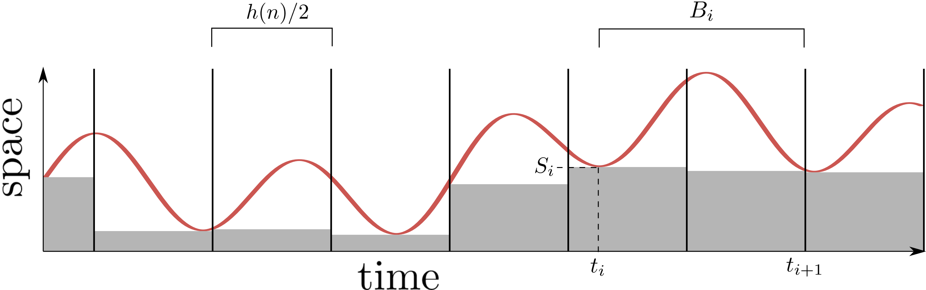
We partition into blocks with large cumulative memory that can only produce a small number of outputs. We achieve this by starting at last unpartitioned layer and finding a suitably low space layer before it so that we can apply Lemma 4.5 to upper bound the number of correct outputs that can be produced in that block with a success probability of at least . Let be the constant from Lemma 4.5 and be the least non-negative integer value of such that the interval:
contains some such that . We recursively define our blocks as follows. Let be the number of blocks generated by this method. The final block starts with the first layer where and ends with layer . Let be the first layer of block . Then the block starts with the first layer where and ends with . See Figure 2 for an illustration of our partitioning. Since we know that . Likewise since when , for all we know that .
Block starts with less than qubits of initial state and has length at most ; so by Lemma 4.5, if , the block can output at most inputs with failure probability at most . Additionally has at least layers so
| (2) |
and each of these layers has at least qubits333This may not hold for with length less than , but Lemma 4.3 gives us that this number of layers is insufficient to find a fixed rank input with probability at least . Thus we can omit such a block from our analysis., so the cumulative memory of is at least so
| (3) |
We now have two possibilities: If we have some such that , the cumulative memory of alone is at least which is and hence has cumulatively memory since . Otherwise, since we require that the algorithm is correct with probability at least , each block can produce at most outputs. Since our circuit must output all elements larger than the median, we know . For convenience we define which allows us to express the constraints as
| (4) |
Minimizing is a non-convex optimization problem and can instead be solved using
| (5) |
for and . Lemma C.1 from Appendix C shows that for non-negative with , we have . Thus and applying the variable substitution gives us: Plugging this into Equation 4 gives us the bound: and hence the cumulative memory of is . ∎
In Appendix B we also show how we can change the length of the blocks to generalize the above proof to arbitrary success probabilities.
5 General methods for proving cumulative memory lower bounds
Our method involves adapting techniques previously used to prove tradeoff lower bounds on worst-case time and worst-case space. We show that the same properties that yield lower bounds on the product of time and space in the worst case can also be used to produce nearly identical lower bounds on cumulative memory. To do so, we first revisit the standard approach to such time-space tradeoff lower bounds.
The standard method for time-space tradeoff lower bounds for multi-output functions
Consider a multi-output function on where the output is either unordered (the output is simply a set of elements from ) or ordered (the output is a vector of elements from ). Then is either the size of the set or the length of the vector of elements. The standard method for obtaining an ordinary time-space tradeoff lower bounds for multi-output functions on -way branching programs is the following:
The part that depends on :
Choose a suitable probability distribution on , often simply the uniform distribution on and then:
- (A)
-
Prove that .
- (B)
-
Prove that for all and any branching program of height , the probability for that produces at least correct output values of on input is at most for some , , , and constant independent of .
Observe that under any distribution , a branching program with ordered outputs that makes no queries can produce outputs that are all correct with probability at least , so the bound in (B) shows that, roughly, up to the difference between and there is not much gained by using a branching program of height .
The generic completion:
In the following outline we omit integer rounding for readability.
-
•
Let and suppose that
(6) -
•
Let , which is at most by hypothesis on , and define .
-
•
Divide time into blocks of length .
-
•
The original branching program can be split into at most sub-branching programs of height , each beginning at a boundary node between layers. By Property (B) and a union bound, for the probability that at least one of these sub-branching programs of height at most produces correct outputs on input is at most by our choice of .
-
•
Under distribution , by (A), with probability at least , an input has some block of time where at least outputs of must be produced on input .
-
•
If , this can occur for at most an fraction of inputs under . Therefore we have and hence since , combining with Equation 6, we have
where is the decision tree complexity of and hence a lower bound on .
Remark 5.1.
Though it will not impact our argument, for many instances of the above outline, the proof of Property (B) is shown for a decision tree of the same height by proving an analog for the conditional probability along each path in the decision tree separately; this will apply to the tree as a whole since the paths are followed by disjoint inputs, so Property (B) follows from the alternative property below:
- (B’)
-
For any partial assignment of output values over and any restriction (i.e., partial assignment) of coordinates within ,
Observe that Property (B’) is only a slightly more general version of Property (*) from the introduction where , is arbitrary, and is used instead of .
Remark 5.2.
The above method still gives lower bounds for many multi-output functions that have individual output values that are easy to compute or large portions of the input space on which they are easy to compute. The bounds follow by applying the method to some subfunction of given by where is a partial assignment to the input coordinates and is a projection onto a subset of output coordinates. In the subsequent discussions we ignore this issue, but the idea can be applied to all of our lower bound methods.
A general extension to cumulative memory bounds
To give a feel for the basic ideas of the method, we first show this for a simple case. Observe that, other than the separate bound on time, the lower bound on cumulative memory usage we prove in this case is asymptotically identical to the bound achieved for the product of time and worst-case space using the standard outline.
Theorem 5.3.
Let . Suppose that properties (A) and (B) apply for , , and . If then the cumulative memory used in computing in time with success probability at least is at least
Proof.
Fix a deterministic branching program of length computing . Rather than choosing fixed blocks of height , layers of nodes at a fixed distance from each other, and a fixed target of outputs per block, we choose the block boundaries depending on the properties of and the target depending on the property of the boundary layer chosen.
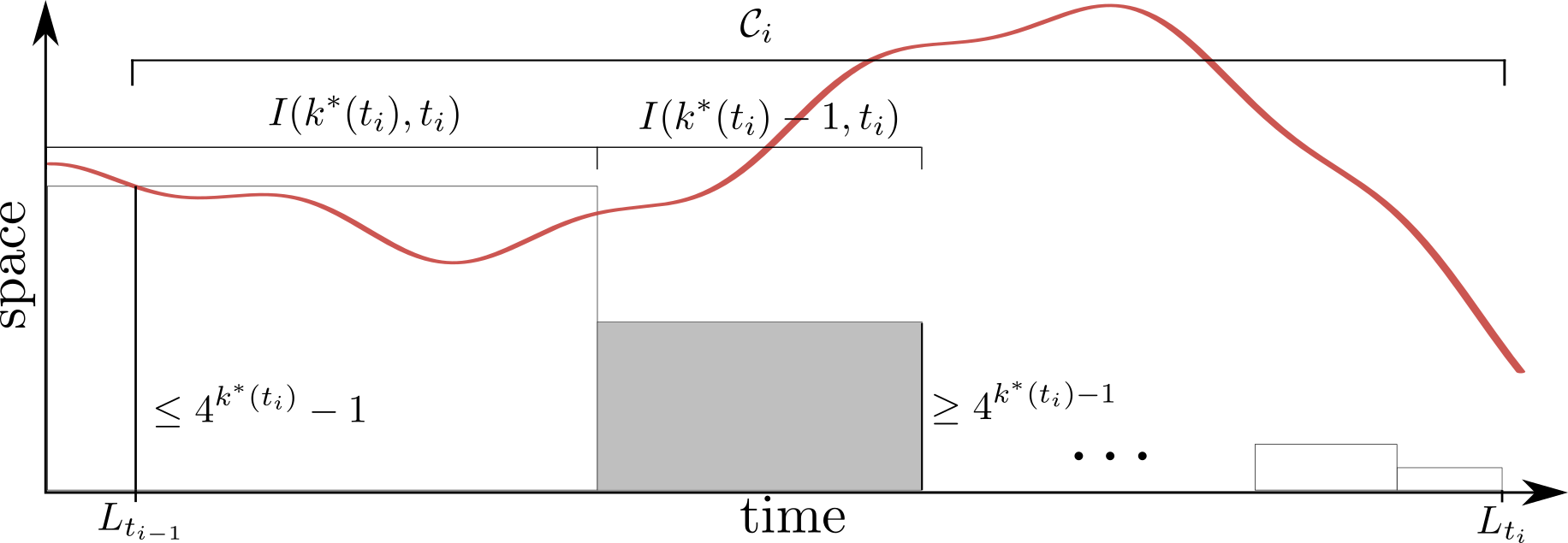
Let . We break into time segments of length working backwards from step so that the first segment may be shorter than the rest. We let and for we let be the time step with the fewest nodes among all time steps .
The -th time block of will be between times and . Observe that by construction so each block has length at most . This construction is shown in Figure 3. Set so that has at nodes. By definition of each , the cumulative memory used by ,
| (7) |
(Note that since , it does not matter that the first segment is shorter than the rest444This simplifies some calculations and is the prime reason for starting the time segment boundaries at rather than at 0..)
We now define the target for the number of output values produced in each time block to be the smallest integer such that . That is,
For , for each and each sub-branching program rooted at some node in and extending until time , by our choice of and Property (B), if , the probability that produces at least correct outputs on input is at most . Therefore, by a union bound, for the probability that produces at least correct outputs in the -th time block on input is at most Therefore, if each , the probability for that there is some such that produces at least correct outputs on input during the -th block is at most . Therefore, if each , the probability for that produces at most correct outputs in total on input is .
If each , since must produce correct outputs on with probability at least , we must have . On the other hand, if some we have the same bound. Using our definition of we have or Plugging in the bound (7) on the cumulative memory and the value of , it implies that or that where the 3 on the right rather than a 2 allows us to remove the ceiling. Therefore either
In the general version of our theorem there are a number of additional complications, most especially because the branching program height limit in Property (B) can depend on , the target for the number of outputs produced. This forces the lengths of the blocks and the space used at the boundaries between blocks to depend on each other in a quite delicate way. In order to discuss the impact of that dependence and state our general theorem, we need the following definition.
Definition 5.4.
Given a non-decreasing function with , we define by . We also define the loss, , of by
Lemma 5.5.
The following hold for every non-decreasing function with :
-
(a)
.
-
(b)
If is a polynomial function then .
-
(c)
For any , .
-
(d)
We say that is nice if it is differentiable and there is an integer such that for all , . If is nice then is . This is tight for with .
We prove these technical statements in Appendix D. Here is our full general theorem.
Theorem 5.6.
Let . Suppose that function defined on has properties (A) and (B) with that is and that is . For , define to be for . Suppose that with and is constant or a differentiable function such that is increasing and concave. Define by
-
(a)
Either which implies that is or the cumulative memory used by a randomized branching program in computing in time with error is at least
-
(b)
Further any randomized random-access machine computing in time with error requires cumulative memory
Before we give the proof of the theorem, we note that by Lemma 5.5, in the case that is constant or for some constant , which together account for all existing applications we are aware of, the function is lower bounded by a constant. In the latter case, is differentiable, has , and the function is increasing and concave so it satisfies the conditions of our theorem. By using , , and with from Property (*) in place of in Property (B’), Theorem 5.6 yields Theorem 1.2.
More generally, the value in the statement of this theorem is at least a constant factor times the value of used in the generic time-space tradeoff lower bound methodology. Therefore, for example, the cumulative memory lower bound derived for random-access machines via Theorem 5.6 is close to the lower bound on the product of time and worst-case space given by standard methods.
Proof of Theorem 5.6.
We prove both (a) and (b) directly for branching programs, which can model random-access machines, and will describe the small variation that occurs in the case that the branching program in question comes from a random-access machine. To prove these properties for randomized branching programs, by Yao’s Lemma [40] it suffices to prove the properties for deterministic branching programs that have error at most under distribution . Fix a (deterministic) branching program of length computing with error at most under distribution . Without loss of generality, has maximum space usage at most space since there are at most inputs.
Let . We break into time segments of length working backwards from step so that the first segment may be shorter than the rest. We then choose a sequence of candidates for the time steps in which to begin new blocks, as follows: We let and for we let
be the time step with the fewest nodes among all time steps . Set so that has at nodes. This segment contributes at least to the cumulative memory bound of .
To choose the beginning of the last time block555Since we are working backwards from the end of the branching program and we do not know how many segments are included in each block, we don’t actually know this index until things stop with . we find the smallest such that . Such a must exist since is a non-decreasing non-negative function, and . We now observe that the length of the last block is at most which by choice of is less than and hence we have satisfied the requirements for Property (B) to apply at each starting node of the last time block.
By our choice of each , the cumulative memory used in the last segments is at least Further, since was chosen as smallest with the above property, we know that for every we have Hence we have and we get a cumulative memory bound for the last segments of at least
| (8) |
Claim 5.7.
.
Proof of Claim.
Observe that it suffices to prove the claim when we replace , which appears on both sides, by a larger quantity. In particular, we show how to prove the claim with instead, which is larger since . But this follows immediately since by definition which is equivalent to what we want to prove. ∎
Write . By the claim, the cumulative memory contribution associated with the last block beginning at is at least
We repeat this in turn to find the time step for the beginning of the next block from the end, . One small difference now is that there is a last partial segment of height at most from the beginning of segment containing to layer . However, this only adds at most to the length of the segment which still remains well within the height bound of for Property (B) to apply.
Repeating this back to the beginning of the branching program we obtain a decomposition of the branching program into some number of blocks, the -th block beginning at time step with nodes, height between and , and with an associated cumulative memory contribution in the -th block of (This is correct even for the partial block starting at time since .) Since we know that , for convenience, we also define for . Then, by definition
| (9) | ||||
| (10) |
As in the previous argument for the simple case, for , we define the target for the number of output values produced in each time block to be the smallest integer such that . That is,
If for some , then since is and and are . Therefore and hence
Suppose instead that for all . Then, for , for each and each sub-branching program rooted at some node in and extending until time , by our choice of and Property (B), the probability that produces at least correct outputs on input is at most Therefore, by a union bound, for the probability that produces at least correct outputs in the -th time block on input is at most
and hence the probability for that there is some such that produces at least correct outputs on input during the -th block is at most . Therefore, the probability for that produces at most correct outputs in total on input is .
Since, by Property (A) and the maximum error it allows, must produce at least correct outputs with probability at least for , we must have . Using our definition of we obtain
This is the one place in the proof where there is a distinction between an arbitrary branching program and one that comes from a random access machine.
We first start with the case of arbitrary branching programs: Note that . Suppose that . Then, even with rounding, we obtain
Unlike an arbitrary branching program that may do non-trivial computation with sub-logarithmic , a random-access machine with even one register requires at least bits of memory (just to index the input for example) and hence will be , since is at most polynomial in without loss of generality and is at most polynomial in by assumption. Therefore we obtain that is without the assumption on .
In the remainder we continue the argument for the case of arbitrary branching programs and track the constants involved. The same argument obviously applies for programs coming from random-access machines with slightly different constants that we will not track. In particular, since for we have
| (11) |
From this point we need to do something different from the argument in the simple case because the lower bound on the total cumulative memory contribution is given by Equation 9 and is not simply . Instead, we combine Equation 11 and Equation 10 using the following technical lemma that we prove in Appendix C.
Lemma 5.8.
Let be a differentiable function such that is a concave increasing function of . For , if and then .
In the special case that (and indeed for any nice function ), there is an alternative variant of the above in which one breaks up time into exponentially growing segments starting with time step . We used that alternative approach in Section 4.
Remark 5.9.
If we restrict our attention to -space bounded computation, then each and the cumulative memory bound for a branching program in Theorem 5.6 becomes And the bound for RAM cumulative memory becomes
Generic method for quantum time-space tradeoffs
Quantum circuit time-space lower bounds have the same general structure as their classical branching program counterparts. They require a lemma similar to (B) that gives an exponentially small probability of producing outputs with a small number of queries.
Lemma 5.10 (Quantum generic property).
For all and any quantum circuit with at most layers, there exists a distribution such that when , the probability that produces at least correct output values of is at most .
Such lemmas have historically been proving using direct product theorems [32, 13] or the recording query technique [29]. Quantum time-space tradeoffs use the same blocking strategy as branching programs; however, they cannot use union bounds to account for input dependent state at the start of a block. Instead, Proposition 4.4 lets us apply Lemma 5.10 to blocks in the middle of a quantum circuit.
The factor in Proposition 4.4 means that a quantum time-space or cumulative memory lower bound will be half of what you would expect from a classical bound with the same parameters. Since a quantum circuit must have qubits to make a query, we know that the space between layers is always at least . Therefore the generic time-space tradeoff for quantum circuits is
where is the bounded-error quantum query complexity of .
Generic method for quantum cumulative complexity bounds
Our generic argument can just as easily be applied to quantum lower bounds for problems where we have an instance of Lemma 5.10 using Proposition 4.4 to bound the number of outputs produced even with initial input-dependent state. Since quantum circuits require at least qubits to hold the query index, the bounds derived are like those from Theorem 5.6(b).
Corollary 5.11.
Let . Suppose that function satisfies generic Lemma 5.10 with that is . For , let . Let where and is constant or a differentiable function where is increasing and concave. Let be defined by:
Then the cumulative memory used by a quantum circuit that computes in time with error is at least
Additionally if the quantum circuit uses qubits, then the cumulative memory bound instead is
6 Applications of our general theorems to classical and quantum computation
Theorems 5.3 and 5.6 are powerful tools that can convert most existing time-space lower bounds into asymptotically equivalent lower bounds on the required cumulative memory. We give a few examples to indicate how our general theorems can be used.
Unique elements
Define by .
Proposition 6.1 (Lemmas 2 and 3 in [16]).
For the uniform distribution on with ,
-
(A)
-
(B’) For any partial assignment of output values over and any restriction of coordinates in , .
The above lemma is sufficient to prove that is for the unique elements problem, and can be easily extended to a cumulative complexity bound using Theorem 5.6.
Theorem 6.2.
For , any branching program computing in time and probability at least requires to be or to be . Further, any random access machine computing with probability at least requires cumulative memory
Proof.
By Proposition 6.1, satisfies conditions (A) and (B) of Section 5 with , , , , and . Since is independent of , the function defined in Theorem 5.6 is the constant function 1 and so . We then apply Theorem 5.6 to obtain the claimed lower bounds. ∎
The above theorem is tight for using the algorithm in [16].
Linear Algebra
We consider linear algebra over some finite field . Let be a subset of with elements.
Definition 6.3.
An matrix is -rigid iff every submatrix where and has rank at least . We call -rigid matrices -rigid.
Matrix rigidity is a robust notion of rank and is an important property for proving time-space and cumulative complexity lower bounds for linear algebra. Fortunately, Abrahamson proved that there are always rigid square matrices.
Proposition 6.4 (Lemma 4.3 in [4]).
There is a constant where at least a fraction of the matrices over are -rigid.
Abrahamson shows in [4] that for any constant and matrix that is -rigid, any -way branching program that computes the function with expected time and expected space666[4] defines expected space as the expected value of the of the largest number of a branching program node that is visited during a computation under best case node numbering. has where . We restate the key property used in that proof.
Proposition 6.5 (Theorem 4.6 in [4]).
Let , be any matrix that is -rigid and be the function over . Let be the uniform distribution on for with . For any restriction of coordinates to values in and any partial assignment of output coordinates over ,
Theorem 6.6.
Let . Let be an matrix over , with that is -rigid. Then, for any -way branching program computing in steps with probability at least , either is or is . Further, computing on a random access machine requires cumulative memory unconditionally.
Proof.
We invoke Theorem 5.3 using Proposition 6.5 to obtain Property (B’) with and . Property (A) is trivial since . ∎
By Proposition 6.4 we know that for some constant , a random matrix has a good chance of being -rigid. This means that computing for a random matrix in time at most is likely to require either the cumulative memory or to be . Since Yesha [41] proved that the DFT matrix is -rigid, the DFT is a concrete example where the cumulative memory or is ; other examples include generalized Fourier transform matrices over finite fields [17, Lemma 28].
Corollary 6.7.
If is an generalized Fourier transform matrix over field with characteristic relatively prime to then any random-access machine computing for where has with probability at least requires cumulative memory that is .
It is easy to see that our lower bound is asymptotically optimal in these cases.
Proposition 6.8 (Theorem 7.1 in [4]).
Let for and be the matrix multiplication function, be the constant from Proposition 6.4, and be the uniform distribution over -rigid matrices. Choose any integers and such that . If then for any -way branching program of height the probability that produces at least correct output values of is at most .
Theorem 6.9.
Multiplying two random matrices in with and with probability at least requires time that is or cumulative memory . On random access machines, the cumulative memory bound is unconditional.
Proof.
Proposition 6.8 lets us apply Theorem 5.6 with , , , , and . This gives us that , so . Then we get that and hence
Therefore we get that either
or, since the loss function for is a constant, the cumulative memory is
Since the decision tree complexity of matrix multiplication is , this is . For random access machines, the same cumulative memory bound applies without the condition on . ∎
Quantum applications of the generic method
Disjoint Collision Pairs Finding
In [29] the authors considered the problem of finding disjoint collisions in a random function , and were able to prove a time-space tradeoff that is for circuits that solve the problem with success probability . Specifically, they consider circuits that must output triples where . To obtain this result, they prove the following theorem using the recording query technique:
Proposition 6.10 (Theorem 4.6 in [29]).
For all and any quantum circuit with at most quantum queries to a random function , the probability that produces at least disjoint collisions in is at most .
The above theorem can be extended to a lemma matching Lemma 5.10 by choosing a sufficiently small constant and setting to obtain a probability of at most . This is sufficient to obtain a matching lower bound on the cumulative memory complexity using Corollary 5.11.
Theorem 6.11.
Finding disjoint collisions in a random function with probability at least requires time is or cumulative memory .
Proof.
Our discussion based on Proposition 6.10 lets us apply Corollary 5.11 with , and . Thus we have and is a differentiable function where is an increasing and concave function. With these parameters, we have:
By Corollary 5.11 with the observation that the loss is constant we get that:
or the quantum cumulative memory is:
By Proposition 6.10 we know that any quantum circuit with at most layers can produce disjoint collisions with probability at most . Thus we know that and our cumulative memory bound becomes . ∎
Linear Inequalities and Boolean Linear Algebra
We now consider problems in Boolean linear algebra where we write for Boolean (i.e. and-or) matrix-vector product and for Boolean matrix multiplication. In [32] the authors prove the following time-space tradeoff for Boolean matrix vector products:
Proposition 6.12 (Theorem 23 in [32]).
For every in , there is an Boolean matrix such that every bounded-error quantum circuit with space at most that computes Boolean matrix vector product in queries requires that is .
This result is weaker than a standard time-space tradeoff since the function involved is not independent of the circuits that might compute it. In particular, [32] does not find a single function that is hard for all space bounds, as the matrix that they use changes depending on the value of . For example, a circuit using space could potentially compute using queries. This means that an extension of their bound to cumulative memory complexity does not follow from our Corollary 5.11, as blocks with distinct numbers of initial qubits would be computing outputs for different functions. In [13] the authors use the same space-dependent matrices to prove a result for systems of linear inequalities.
Proposition 6.13 (Theorem 19 in [13]).
Let be in and be the all- vector. There is an Boolean matrix such that every bounded error quantum circuit using space for evaluating the system using queries requires that is .
Again this result is not a general time-space tradeoff and hence is not compatible with obtaining a true cumulative memory bound777The analogous cumulative complexity result would require the matrix to depend extensively on the structural properties of the circuit, including the number of qubits after each layer and the locations of each fixed output gate. It is unclear whether the TS results also may need the matrix to depend on the locations of the output gates.. While neither of the above results is a time-space tradeoff for a fixed function, [32] leverages the ideas for Proposition 6.12 to compute a true time-space tradeoff lower bound for computing Boolean matrix multiplication.
Proposition 6.14 (Theorem 25 in [32]).
If a quantum circuit computes the Boolean matrix product with bounded error using queries and space, then is .
In Proposition 6.14, unlike in Proposition 6.12 and Proposition 6.13, both and are inputs to the problem. This allows the lower bound argument to use the properties of the circuit to find matrices and for which the circuit will be particularly challenged. More precisely, to prove the above result, the authors use a lemma matching the form of Lemma 5.10 that we extract from their lower bound argument.
Proposition 6.15 (from Theorem 25 in [32]).
Let be any fixed set of outputs to the function . Then there are constants such that for any quantum circuit with at most layers, there is a distribution over pairs of matrices such that when , the probability that produces the correct values for is at most .
Note that, though there are total output values, Proposition 6.15 only works when k — the number of output values in a block — is sublinear in . This is not a problem in the time-space tradeoff lower bound. Proposition 6.15 upper bounds the value of for a block as . Since the time must be simply to read the input, the bound trivially holds when is . Thus the time-space tradeoff proof only needs to apply Proposition 6.15 when (and therefore ) is sublinear in .
We cannot apply such an argument when considering cumulative memory complexity, as a circuit can use qubits for a small number of layers without having an asymptotic effect on the cumulative memory complexity. However, if we consider space bounded computation, we can get a matching bound on the cumulative memory complexity.
Theorem 6.16.
Any quantum circuit that computes the Boolean matrix product requires ancilla qubits or cumulative memory that is .
Proof.
Proposition 6.15 lets us apply Corollary 5.11 with being , and . Thus we have and . Therefore we define to be
Thus by Corollary 5.11 we get that the space bound is or the cumulative memory is . ∎
Though this is somewhat limited in its range of applicability, it still yields a generalization of the time-space tradeoff lower bound of Proposition 6.14 when is .
7 Cumulative memory complexity of single-output functions
The time-space tradeoff lower bounds known for classical algorithms computing single-output functions are quite a bit weaker than those for multi-output functions, but the bounds we can obtain on cumulative memory for slightly super-linear time bounds are nearly as strong as those for multi-output functions.
For simplicity we focus on branching programs with Boolean output, in which case, we can simply assume that the output is determined by which of two nodes the branching program reaches at time step .
The general method for bounds for single output functions is based on the notion of the trace of a branching program computation. We fix a branching program computing . As in the case of the simple bounds for multi-output functions, we break up into a sequence of blocks, say of them, that are separated by time steps . A trace in is a sequence of nodes of , one node in the set of nodes at time step for each . The set of all traces .
A key object under consideration is the notion of an embedded rectangle, which is a subset of with associated disjoint subsets and with and assignment such that . We write .
Proposition 7.1 (Implicit in Corollary 5.2 of [18]).
Let be a branching program of length computing a function . Suppose that for and . If are time steps with , then there is an embedded rectangle with and where is the set of traces of associated with time steps .
Corollary 7.2.
Let be a -way branching program of length computing a function . If for and , then there is an embedded rectangle with and .
Proof.
Fix a branching program of length computing . We can extend to length exactly by adding a chain of nodes to the root. This does not impact the cumulative memory bound of – a single node per level is 0 space – so we assume that without loss of generality. Let . We apply the same basic idea for the choice of time steps used in the simple general method for multi-output functions: Namely, we break into time segments of length either or . We define and define for to be the time step during the next segment at which the set is minimized. Write . Then the cumulative memory complexity used by satisfies
since .
Clearly each is at most by definition, since their difference is at most the length of two consecutive time segments. Therefore, the conditions of Proposition 7.1 apply and we obtain that there is an embedded rectangle with and
An example of a natural problem that we can apply this to is the Hamming Closeness problem which outputs 1 iff there is a pair of input coordinates such that the Hamming distance between the binary representations of and is at most .
Proposition 7.3 ([18]).
For , and we have
-
•
(Proposition 6.15) , and
-
•
(Lemma 6.17) there is a constant such that any embedded rectangle has .
We can apply the above to prove that any -way branching program computing for in time and space requires that is .
Theorem 7.4.
For any -way branching program computing in time that is requires cumulative memory which is .
Proof.
Let be an -way branching program computing in time that is . We can swap the sink nodes to obtain a branching program computing . Write and assume wlog that . Therefore is and hence is and hence . Therefore by Corollary 7.2, there is an embedded rectangle such that and
Therefore by Proposition 7.3, for some constant we have
Since , solving we obtain
Since is we obtain that for some constant . Therefore, plugging in the value of for , we see that is . This is by the bound on . ∎
Similar bounds can also be shown by related means for various problems involving computation of quadratic forms, parity-check matrices of codes and others. For some problems the following stronger lower bound method is required.
Proposition 7.5 (Implicit in Corollary 5.4 of [18]).
Let be a -way branching program of length computing a function . Suppose that for and for . If are time steps with , then there is an embedded rectangle with and where is the set of traces of associated with time steps .
Corollary 7.6.
Let be a branching program of length computing a function . If for and for , then there is an embedded rectangle with and .
Proof Sketch.
The proof is the analog of that of Corollary 7.2 using Proposition 7.5 in place of Proposition 7.1. ∎
Define the Element Distinctness function on to be the Boolean function that is 1 iff all values in the input are distinct.
Proposition 7.7 ([18]).
For ,
-
•
(Proposition 6.11) , and
-
•
(Lemma 6.12) Every embedded rectangle in has .
[18] used this to prove that the time and space for computing must satisfy . We strengthen this to the following theorem using Corollary 7.6.
Theorem 7.8.
Any -way branching program computing in time that is requires cumulative memory which is .
Proof.
Let compute in time that is . Write so that and assume wlog that . Write . Since is , is and which is and hence and therefore . We can then apply Corollary 7.6 to say that there is a rectangle with and . By Proposition 7.7, we have
Solving, we obtain that
Therefore, since , we have constant such that . As noted above, is . More precisely, the bound we obtain is
8 Acknowledgements
Many thanks to David Soloveichik for his guidance and contributions to our initial results. Thanks also to Scott Aaronson for encouraging us to consider cumulative memory complexity in the context of quantum computation.
References
- [1] Scott Aaronson. Limitations of quantum advice and one-way communication. Theory of Computing, 1(1):1–28, 2005. doi:10.4086/toc.2005.v001a001.
- [2] Karl R. Abrahamson. Generalized string matching. SIAM J. Comput., 16(6):1039–1051, 1987. doi:10.1137/0216067.
- [3] Karl R. Abrahamson. A time-space tradeoff for Boolean matrix multiplication. In 31st Annual IEEE Symposium on Foundations of Computer Science, Volume I, pages 412–419, 1990. doi:10.1109/FSCS.1990.89561.
- [4] Karl R. Abrahamson. Time-space tradeoffs for algebraic problems on general sequential machines. J. Comput. Syst. Sci., 43(2):269–289, 1991. doi:10.1016/0022-0000(91)90014-v.
- [5] Miklós Ajtai. Determinism versus nondeterminism for linear time RAMs with memory restrictions. J. Comput. Syst. Sci., 65(1):2–37, 2002. doi:10.1006/jcss.2002.1821.
- [6] Miklós Ajtai. A non-linear time lower bound for Boolean branching programs. Theory Comput., 1(1):149–176, 2005. doi:10.4086/toc.2005.v001a008.
- [7] Joël Alwen and Jeremiah Blocki. Efficiently computing data-independent memory-hard functions. In Advances in Cryptology – CRYPTO 2016, pages 241–271, 2016.
- [8] Joël Alwen, Jeremiah Blocki, and Krzysztof Pietrzak. Depth-robust graphs and their cumulative memory complexity. In Advances in Cryptology – EUROCRYPT 2017, pages 3–32, 2017.
- [9] Joël Alwen, Binyi Chen, Chethan Kamath, Vladimir Kolmogorov, Krzysztof Pietrzak, and Stefano Tessaro. On the complexity of Scrypt and proofs of space in the parallel random oracle model. In Advances in Cryptology - EUROCRYPT 2016, Proceedings, Part II, volume 9666 of LNCS, pages 358–387, 2016. doi:10.1007/978-3-662-49896-5_13.
- [10] Joël Alwen, Binyi Chen, Krzysztof Pietrzak, Leonid Reyzin, and Stefano Tessaro. Scrypt is maximally memory-hard. In Advances in Cryptology - EUROCRYPT 2017, Proceedings, Part III, volume 10212 of Lecture Notes in Computer Science, pages 33–62, 2017. doi:10.1007/978-3-319-56617-7_2.
- [11] Joël Alwen, Susanna F. de Rezende, Jakob Nordström, and Marc Vinyals. Cumulative space in black-white pebbling and resolution. In 8th Innovations in Theoretical Computer Science Conference (ITCS 2017), volume 67 of Leibniz International Proceedings in Informatics (LIPIcs), pages 38:1–38:21, 2017. doi:10.4230/LIPIcs.ITCS.2017.38.
- [12] Joël Alwen and Vladimir Serbinenko. High parallel complexity graphs and memory-hard functions. In Proceedings of the Forty-Seventh Annual ACM Symposium on Theory of Computing, page 595–603, 2015. doi:10.1145/2746539.2746622.
- [13] Andris Ambainis, Robert Špalek, and Ronald de Wolf. A new quantum lower bound method, with applications to direct product theorems and time-space tradeoffs. Algorithmica, 55(3):422–461, 2009. doi:10.1007/s00453-007-9022-9.
- [14] Mohammad Hassan Ameri, Alexander R. Block, and Jeremiah Blocki. Memory-hard puzzles in the standard model with applications to memory-hard functions and resource-bounded locally decodable codes. Cryptology ePrint Archive, Paper 2021/801, 2021. arXiv:https://eprint.iacr.org/2021/801.
- [15] Andrew Baird, Bryant Bost, Stefano Buliani, Vyom Nagrani, Ajay Nair, Rahul Popat, and Brajendra Singh. AWS serverless multi-tier architectures with Amazon API Gateway and AWS Lambda, 2021. arXiv:https://docs.aws.amazon.com/whitepapers/latest/serverless-multi-tier-architectures-api-gateway-lambda/welcome.html.
- [16] Paul Beame. A general sequential time-space tradeoff for finding unique elements. SIAM J. Comput., 20(2):270–277, 1991. doi:10.1137/0220017.
- [17] Paul Beame, T. S. Jayram, and Michael E. Saks. Time-space tradeoffs for branching programs. J. Comput. Syst. Sci., 63(4):542–572, 2001. doi:10.1006/jcss.2001.1778.
- [18] Paul Beame, Michael E. Saks, Xiaodong Sun, and Erik Vee. Time-space trade-off lower bounds for randomized computation of decision problems. J. ACM, 50(2):154–195, 2003. doi:10.1145/636865.636867.
- [19] Jeremiah Blocki and Samson Zhou. On the depth-robustness and cumulative pebbling cost of Argon2i. In Theory of Cryptography, pages 445–465, 2017.
- [20] Dan Boneh, Henry Corrigan-Gibbs, and Stuart Schechter. Balloon hashing: A memory-hard function providing provable protection against sequential attacks. In Advances in Cryptology – ASIACRYPT 2016, pages 220–248, 2016.
- [21] Allan Borodin and Stephen A. Cook. A time-space tradeoff for sorting on a general sequential model of computation. SIAM J. Comput., 11(2):287–297, 1982. doi:10.1137/0211022.
- [22] Allan Borodin, Michael J. Fischer, David G. Kirkpatrick, Nancy A. Lynch, and Martin Tompa. A time-space tradeoff for sorting on non-oblivious machines. J. Comput. Syst. Sci., 22(3):351–364, 1981. doi:10.1016/0022-0000(81)90037-4.
- [23] Allan Borodin, Alexander A. Razborov, and Roman Smolensky. On lower bounds for read-k-times branching programs. Comput. Complex., 3:1–18, 1993. doi:10.1007/BF01200404.
- [24] Ashok K. Chandra, Merrick L. Furst, and Richard J. Lipton. Multi-party protocols. In Proceedings of the Fifteenth Annual ACM Symposium on Theory of Computing, page 94–99, 1983. doi:10.1145/800061.808737.
- [25] Binyi Chen and Stefano Tessaro. Memory-hard functions from cryptographic primitives. In Advances in Cryptology – CRYPTO 2019, pages 543–572, 2019.
- [26] Stephen A. Cook. An observation on time-storage trade off. In Proceedings of the Fifth Annual ACM Symposium on Theory of Computing, STOC ’73, page 29–33, New York, NY, USA, 1973. Association for Computing Machinery. doi:10.1145/800125.804032.
- [27] Cynthia Dwork, Moni Naor, and Hoeteck Wee. Pebbling and proofs of work. In Advances in Cryptology – CRYPTO 2005, pages 37–54, 2005.
- [28] Stefan Dziembowski, Tomasz Kazana, and Daniel Wichs. One-time computable self-erasing functions. In Theory of Cryptography, pages 125–143, 2011.
- [29] Yassine Hamoudi and Frédéric Magniez. Quantum time-space tradeoff for finding multiple collision pairs. In 16th Conference on the Theory of Quantum Computation, Communication and Cryptography (TQC 2021), volume 197 of Leibniz International Proceedings in Informatics (LIPIcs), pages 1:1–1:21, 2021. doi:10.4230/LIPIcs.TQC.2021.1.
- [30] Stasys Jukna. A nondeterministic space-time tradeoff for linear codes. Inf. Process. Lett., 109(5):286–289, 2009. doi:10.1016/j.ipl.2008.11.001.
- [31] Nikolaos P. Karvelas and Aggelos Kiayias. Efficient proofs of secure erasure. In Security and Cryptography for Networks, pages 520–537, 2014.
- [32] Hartmut Klauck, Robert Špalek, and Ronald de Wolf. Quantum and classical strong direct product theorems and optimal time‐space tradeoffs. SIAM Journal on Computing, 36(5):1472–1493, 2007. doi:10.1137/05063235x.
- [33] Yishay Mansour, Noam Nisan, and Prasoon Tiwari. The computational complexity of universal hashing. Theor. Comput. Sci., 107(1):121–133, 1993. doi:10.1016/0304-3975(93)90257-T.
- [34] E. Okol’nishnikova. On lower bounds for branching programs. Siberian Advances in Mathematics, 3(1):152–166, 1993.
- [35] Nicholas Pippenger. On simultaneous resource bounds (preliminary version). In 20th Annual IEEE Symposium on Foundations of Computer Science, pages 307–311, 1979. doi:10.1109/SFCS.1979.29.
- [36] Ling Ren and Srinivas Devadas. Proof of space from stacked expanders. In Proceedings, Part I, of the 14th International Conference on Theory of Cryptography - Volume 9985, page 262–285. Springer-Verlag, 2016. doi:10.1007/978-3-662-53641-4_11.
- [37] Martin Sauerhoff and Philipp Woelfel. Time-space tradeoff lower bounds for integer multiplication and graphs of arithmetic functions. In Proceedings of the 35th Annual ACM Symposium on Theory of Computing, pages 186–195, 2003. doi:10.1145/780542.780571.
- [38] John E. Savage. Models of Computation: Exploring the Power of Computing. Addison-Wesley Longman Publishing Co., Inc., USA, 1st edition, 1997.
- [39] Martin Tompa. Time-space tradeoffs for computing functions, using connectivity properties of their circuits. J. Comput. Syst. Sci., 20(2):118–132, 1980. doi:10.1016/0022-0000(80)90056-2.
- [40] Andrew Chi-Chih Yao. Probabilistic computations: Toward a unified measure of complexity (extended abstract). In 18th Annual IEEE Symposium on Foundations of Computer Science, pages 222–227, 1977. doi:10.1109/sfcs.1977.24.
- [41] Yaacov Yesha. Time-space tradeoffs for matrix multiplication and the discrete Fourier transform on any general sequential random-access computer. Journal of Computer and System Sciences, 29(2):183–197, 1984. doi:10.1016/0022-0000(84)90029-1.
- [42] Mark Zhandry. How to record quantum queries, and applications to quantum indifferentiability. In Advances in Cryptology – CRYPTO 2019, pages 239–268, 2019.
Appendix A A gap between time-space product and cumulative memory
Here we discuss some commonly studied structured sequential models of computation with provable separations between time-space and cumulative memory complexities.
Black pebbling separation
Definition A.1.
The black pebble game is a one player game played on a graph with source nodes and target nodes . The game is played by placing and removing pebbles from the graph according to the following rules:
-
•
A pebble may be placed on any source node .
-
•
A pebble may be placed on any node whose immediate predecessors all have pebbles.
-
•
A pebble may be moved from a node to one of its children if all other parents of that node contain pebbles.
-
•
A pebble may be removed from any node.
The goal of the game is to simultaneously have pebbles on each node . The time of a pebbling is the number of steps taken and the pebbles is the largest number of pebbles placed on the graph at any time. We say that the time-space of a pebbling is the product of its time and number of pebbles. The cumulative memory of a pebbling is the sum of the number of pebbles placed after each step.
We will be considering instances of the black pebble game where contains exactly the unique node with in-degree zero and contains exactly the unique node with out-degree zero. Intuitively, the black pebble game corresponds to strategies for evaluating straight line programs, where a pebble indicates that a particular value has been computed and is currently stored in memory. Thus the number of pebbles used when pebbling a graph is analogous to the space used by that computation. We will construct a simple DAG where the time-space complexity is larger than the cumulative memory complexity.
Proposition A.2.
There is a family of DAGs such that graph requires pebbles and steps to pebble but can be pebbled with cumulative memory .
Hence there is an separation between the time-space product and cumulative memory for pebbling.
Proof.
We construct , as shown in Figure 4, to contain an square lattice whose node of out-degree zero now has an out-going edge to the head of a chain containing nodes. Since pebbling the lattice requires pebbling a pyramid of height , Theorem 5 of [26] tells us that pebbles are necessary to place a pebble at the end of the lattice. Since a pebble must be placed on each node in the chain of length , pebbling this graph takes at least steps.

Now we will show how this graph can be pebbled with less cumulative memory. We will show that both the lattice and the chain can each be pebbled with cumulative memory that is . The lattice can be pebbled by placing pebbles along the top diagonal and then repeatedly moving these pebbles along their downward edges until they are all on the bottom diagonal. This uses pebbles and acts on each node exactly once for a total of steps. Thus the cumulative memory for pebbling the lattice is . For the chain we can simply move one pebble from the leftmost node to the rightmost node in steps. Since this process only requires one pebble, the cumulative memory is also . ∎
Random oracle separation
There is a group of closely related theorems from cryptography that let us instantiate pebbling graphs with the help of a random oracle [27, 28, 31]. Here we walk through the ideas behind these proofs to show that the graph in Proposition A.2 leads to separation between time-space and cumulative memory complexities in the random oracle model. The concrete problem we will be considering is related to labeling nodes of the pebbling graph.
Definition A.3.
Let be a DAG with maximum in-degree two and target . Fix to be some large constant. Let be a random function. We assign each a label as follows:
-
•
If has in-degree zero, then .
-
•
If has exactly one parent , then .
-
•
If has two parents where , then .
The hash-graph problem is the task of computing the label of .
We will use the notation to denote an algorithm that has query access to the random oracle (function) . We start by proving a weaker version of a result in [27].
Definition A.4 ([27]).
Let be a DAG and be an algorithm that solves the hash-graph problem . Then the ex post facto pebbling of is defined as follows:
-
•
Making the call when has in-degree zero corresponds to placing a pebble on .
-
•
Making the call when ’s only parent is corresponds to placing a pebble on .
-
•
Making the call when and are the parents of and corresponds to placing a pebble on .
-
•
A pebble is remove as soon as it is no longer needed. This happens when either the children of that node are never pebbled after this point or when the node is pebbled again before any of its children are pebbled.
Analyzing ex post facto pebbling is key to the arguments in [27, 28, 31] and lets us lower bound the space required to compute a hash-graph.
Proposition A.5 ([27]).
Consider an algorithm that operates for a certain number of steps with bits of memory. Then with probability at least (over the choice of ) the maximum number of pebbles placed by the ex post facto pebbling of is bounded above by .
This lets us show that a hash-graph problem requires at least as much time and space as pebbling its underlying graph, as we show below in an argument similar to ones in [28, 31].
Proposition A.6.
Let be a DAG that requires pebbles and steps to pebble. Then any algorithm that solves the hash-graph problem must use space that is larger than and time that is at least or its success probability (over the randomness of ) is at most .
Proof.
For an algorithm with space bound to solve , one of the following events must happen:
-
1.
solves without placing a pebble on the target during the ex post facto pebbling.
-
2.
places pebbles during the ex post facto pebbling.
-
3.
places a pebble during the ex post facto pebbling that would not be valid according to the black pebble game.
Since is a random oracle, (1) happens with probability at most . By Proposition A.5 (2) happens with probability at most . Since guessing a label that has not been pebbled is possible with probability at most , We know that (3) happens with probability at most via a union bound over the queries of and the nodes of . Thus by a union bound, the probability can produce the correct output is at most which in turn is at most .
Now consider an algorithm with time bound . Since cannot be pebbled in this number of steps, one of the following events must happen for to produce the correct output:
-
1.
solves without placing a pebble on the target during the ex post faco pebbling.
-
2.
places a pebble during the ex post facto pebbling that would not be valid according to the black pebble game.
Both of the events are the same as in the space bounded case, and therefore a union bound give a success probability of at most . ∎
Thus any algorithm that solves must obey the space and the time bounds imposed by pebbling that graph or spend time that is .888Since is an arbitrary constant, this time bound can be made arbitrarly large. Note that a pebbling of a graph directly corresponds to a strategy for computing with the same space, time, and cumulative memory bounds as the pebbling. By using the graph from Proposition A.2, this gives us a separation between time-space product complexity and cumulative memory in the random oracle model.
Corollary A.7.
Relative to a random oracle , there is a problem with an separation between its time-space product complexity and its cumulative memory complexity.
While this will be hard to prove, we believe that replacing the random oracle with a suitable hash function gives a problem where there is an asymptotic gap between these complexity measures.
Conjecture A.8.
Instantiating the family of DAGs from Proposition A.2 as hash-graph problems with some concrete hash-function gives a problem with an unconditional asymptotic gap between its sequential time-space product and cumulative memory complexities.
Appendix B Quantum sorting with arbitrary success probability
In order to modify Theorem 4.6 for different success probabilities, the key is to choose a different value for the parameter in Proposition 4.2 governing the completeness bound, which will change the corresponding value of and . If we want to deal with non-constant values of , it is important to understand how and are related in Proposition 4.2. The following lemma is sufficient to prove Theorem 13 in [32] (our Proposition 4.2). Although the authors of [32] prove a more general version of this proposition, the statement below captures what is necessary in our proof. Specifically, we invoke their Lemma 12 where and .
Proposition B.1 (Special case of Lemma 12 in [32]).
Let be a degree univariate polynomial such that:
-
•
when
-
•
-
•
when
Then there exists universal positive constants and such that for any where :
The in this bound gives the completeness bound on the -threshold problem. We now prove that is sufficiently small when .
Lemma B.2.
Let be the constants from Proposition B.1. When we have , the completeness bound for the -threshold problem with queries is less than .
Proof.
By Proposition B.1 we have
| (12) |
We first bound the first term in the numerator
Next we bound the second term in the numerator
Plugging these bounds into (12) we get
We now describe how to substitute the bound of Lemma B.2 in place of Proposition 4.2 to yield cumulative memory lower bounds for quantum circuits with failure probability at most : To prove the analog of Lemma 4.5, for any , , and , we can reprove a more precise version of Lemma 4.3 using Lemma B.2 instead of Proposition 4.2 to bound the success probability for the -threshold problem and choose
to get a success probability of less than for circuits with as many as
layers and qubits of advice to produce outputs. If we repeat the proof of Theorem 4.6 for failure probability less than , we can set to a value that is to obtain a lower bound on the cumulative memory that is .
Appendix C Optimizations
In this section we prove general optimization lemmas that allow us to derive worst-case properties of the allocation of branching program layers into blocks.
The first special case is relevant for our analysis of quantum sorting algorithms.
Lemma C.1.
For non-negative reals if then .
Proof.
Without loss generality we remove all that are 0 or 1 since they contribute the same amount to each of , , and . Therefore every satisfies or it satisfies . We rename those with by and those with by .
Then can be rewritten as , and both quantities are positive. Let be the largest value and be the smallest value . Thus:
Rewriting gives or , as required. ∎
The following is a generalization of the above to all differentiable functions such that is a concave increasing function of .
See 5.8
Proof.
By hypothesis, . Observe that is an increasing function of since is an increasing function of that is 0 precisely when . Since all with evaluate to 0 in the sum, we can rewrite it as
| (13) |
where each of the summed terms is positive. For , define
Observe that for the denominator is 0 and the numerator equals which is also 0. For both the numerator and denominator are positive and for both the numerator and denominator are negative. Hence is non-negative for every .
Claim C.2.
If is a convex differentiable function, we can complete to a (non-decreasing) continuous function of with for all with
Proof of Claim.
Write . Then since and , we have
Therefore
Since the denominator is a square and is increasing, to prove that for it suffices to prove that the numerator is non-negative.
Suppose first that , Then and the numerator if and only if , which is equivalent to the slope of the tangent to at being at least that of the chord from to . This is certainly true since is a concave function.
Suppose now that . Then and the numerator if and only if . Again, this is true since is a concave function.
It remains to show that we can complete to a continuous function by giving it a finite value at . By l’Hôpital’s rule, the limit of as approaches is
if the denominator is non-zero, which it is, since is an increasing differentiable function at . ∎
We now have the tools we need. Let be the largest and be the smallest . Then we have and
Adding back the terms where , which have value 0, and rewriting we obtain
Therefore we have
Appendix D Proof of Lemma 5.5
See 5.5
Proof.
Since is non-decreasing, for and hence
| (14) |
since is included in the numerator. is the minimum over all integers of and is non-decreasing so we have , which proves part (a)
When we have
so each term in the definition of is larger than which proves part (b). (More precise bounds can be shown but we are not focused on the specific constant.)
Let be an integer. Then . Observe that there are at least integers with . Therefore
| (15) |
The minimum over all is equivalent to the minimum over all , which proves part (c).
Now suppose that is nice. Since is differentiable, for any ,
Then by induction we have that for every positive integer , . Write . Then and
or equivalently that and hence
since is a non-decreasing function. Applying the lower bound from Equation 14 when and the lower bound from Equation 15 when we obtain
Since is a constant, we obtain that is .
Observe that given by is nice for every constant since . In this case we have and since the largest term in each numerator is (a little) more than the sum of all smaller terms put together. Together with the lower bound, this proves part (d). ∎