Impact of high-scale Seesaw and Leptogenesis on inflationary tensor perturbations as detectable gravitational waves

Abstract

We discuss the damping of inflationary gravitational waves (GW) that re-enter the horizon before or during an epoch, where the energy budget of the universe is dominated by an unstable right handed neutrino (RHN), whose out of equilibrium decay releases entropy. Starting from the minimal Standard Model extension, motivated by the observed neutrino mass scale, with nothing more than 3 RHN for the Seesaw mechanism, we discuss the conditions for high scale leptogenesis assuming a thermal initial population of RHN. We further address the associated production of potentially light non-thermal dark matter and a potential component of dark radiation from the same RHN decay. One of our main findings is that the frequency, above which the damping of the tensor modes is potentially observable, is completely determined by successful leptogenesis and a Davidson-Ibarra type bound to be at around $0.1\text{\,}\mathrm{Hz}$. To quantify the detection prospects of this GW background for various proposed interferometers such as AEDGE, BBO, DECIGO, Einstein Telescope or LISA we compute the signal-to-noise ratio (SNR). This allows us to investigate the viable parameter space of our model, spanned by the mass of the decaying RHN $M_{1}\gtrsim$2.4\text{\times}{10}^{8}\text{\,}\mathrm{GeV}$\cdot\sqrt{$2\text{\times}{10}^{-7}\text{\,}\mathrm{eV}$/\tilde{m}_{1}}$ (for leptogenesis) and the effective neutrino mass parameterizing its decay width $\tilde{m}_{1}<$2.9\text{\times}{10}^{-7}\text{\,}\mathrm{eV}$$ (for RHN matter domination). Thus gravitational wave astronomy is a novel way to probe both the Seesaw and the leptogenesis scale, which are completely inaccessible to laboratory experiments in high scale scenarios.

1 Introduction

The standard model (SM) of particle physics predicts that the neutrinos are massless, but due to the observation of neutrino oscillations for solar dc27cfb ; Super-Kamiokande:2001bfk ; Super-Kamiokande:2002ujc ; SNO:2002tuh ; Super-Kamiokande:2005mbp ; articleKam ; PhysRevD.94.052010 ; Borexino:2015axw , atmospheric IceCube:2017lak ; ANTARES:2018rtf and reactor KamLAND:2008dgz ; T2K:2011ypd ; DoubleChooz:2011ymz ; T2K:2013ppw neutrinos we now know that they are massive and the flavor states mix due to the propagation of multiple mass eigenstates. Moreover the $\beta$-decay experiment KATRIN KATRIN:2021uub has provided us with the first direct limit of the neutrino mass scale $m_{\nu}<$0.8\text{\,}\mathrm{eV}$$. Cosmology offers an indirect probe of this scale and demands that the sum of all neutrino masses satisfies $\sum_{i}m_{\nu_{i}}<$0.12\text{\,}\mathrm{eV}$$ Aghanim:2018eyx ; eBOSS:2020yzd in order to be consistent with the predictions for the Cosmic Microwave Background (CMB) radiation, Large scale structure (LSS) formation and Big Bang Nucleosynthesis (BBN). The accelerated expansion at the beginning of the universe provided by cosmic inflation, which was postulated in order to solve the horizon and the flatness problems and is responsible for quantum generation of the primordial fluctuations seeding the large scale structure of the universe, is thought to be driven by a scalar field known as the inflaton (see Martin:2013tda for a review). In this paper, we will be concerned with the primordial Gravitational Waves (GW) background of such inflationary origin Grishchuk:1974ny ; Starobinsky:1979ty ; Rubakov:1982df (see Guzzetti:2016mkm for a review on this topic). These inflationary GWs can act as a logbook of the expansion history of our universe throughout its entire evolution Seto:2003kc ; Boyle:2005se ; Boyle:2007zx ; Kuroyanagi:2008ye ; Nakayama:2009ce ; Kuroyanagi:2013ns ; Jinno:2013xqa ; Saikawa:2018rcs . Particularly, the detailed time evolution of the Hubble rate during the expansion determines the transfer function that describes how gravitational waves at different frequencies are red-shifted to the present day. This property turns primordial GWs into a powerful tool that grants access to the thermal history of our universe prior to BBN. Primordial GWs offer, e.g. an opportunity to measure the reheating temperature after inflation Bernal:2020ywq ; Nakayama:2008ip ; Nakayama:2008wy ; Kuroyanagi:2011fy ; Buchmuller:2013lra ; Buchmuller:2013dja ; Jinno:2014qka ; Kuroyanagi:2014qza . Similarly, with help of these inference can be drwan of the equation of state during the quark-hadron phase transition in quantum chromodynamics Schettler:2010dp ; Hajkarim:2019csy or constrain properties of the hidden sectors beyond the Standard Model (BSM) of particle physics Jinno:2012xb ; Caldwell:2018giq .

The observed baryon asymmetry of the universe (BAU) is longstanding puzzle in particle physics and cosmology Zyla:2020zbs ; Aghanim:2018eyx . While the universe is expected to start in a matter-antimatter symmetric phase, any primordial asymmetry set due tothe initial conditions is expected to get diluted by the exponential expansion phase during cosmic inflation. The BAU is often quoted in terms of the baryon to photon ratio measurement which, according to the latest Planck 2018 data, is given by Aghanim:2018eyx

$$\eta_{B}=\frac{n_{B}-n_{\bar{B}}}{n_{\gamma}}=6.1\times 10^{-10}$$ (1)

and agrees with the value extracted from BBN Fields:2019pfx as well. Similar to the BAU, there has been another question related to the presence of a mysterious, non-luminous form of matter, popularly known as dark matter (DM), giving rise to approximately $26\%$ of the energy density in the present universe. In terms of density parameter $\Omega_{\rm DM}$ and $h=H_{0}/(100\;\text{km}~{}\text{s}^{-1}\text{Mpc}^{-1})$ with $H_{0}$ being the observed present day Hubble parameter, the current DM abundance is conventionally reported to be Aghanim:2018eyx

$$\Omega_{\text{DM}}h^{2}=0.120\pm 0.001$$ (2)

at 68% CL. Apart from cosmological evidence, the presence of DM has also been suggested by several astrophysical implications Zwicky:1933gu ; Rubin:1970zza ; Clowe:2006eq . While none of the standard model particles satisfy the criteria of a particle DM candidate, the SM also does not to satisfy the criteria to dynamically generate the observed BAU, known as Sakharov’s conditions Sakharov:1967dj , in adequate amounts. This has led to several BSM possibilities offering intriguing solutions to these puzzles: The Type I Seesaw mechanism Minkowski:1977sc ; Yanagida:1979as ; Gell-Mann:1979vob ; Glashow:1979nm ; 10.1143/PTP.64.1103 ; PhysRevLett.44.912 , where the SM is augmented with three right handed SM gauge singlet neutrinos (RHN), may explain both the observed neutrino masses (from neutrino oscillation experiments) as well as the baryon asymmetry of the universe via first generating an asymmetry in the dark leptonic sector Fukugita:1986hr ; Luty:1992un ; Plumacher:1996kc ; Covi:1996wh ; Giudice:2003jh and subsequently getting transferred to the visible baryonic sector via the electroweak sphaleron transitions Kuzmin:1985mm . Among the BSM proposals for DM, the weakly interacting massive particle (WIMP) Kolb:1990vq produced as a thermal relic is perhaps the most widely studied one (see Arcadi:2017kky for a review). However due to the absence of any WIMP related signals in nuclear and electron recoil DM direct detection experiments, there has been growing interest in other (non-thermal) production modes: some examples are the well-known super-WIMP scenario Feng:2003xh , where frozen out WIMP decays to the actual DM, FIMPs Hall:2009bx (see Bernal:2017kxu for a review) that have such tiny couplings to the SM plasma that they never thermalize, or non-thermal production from inflaton decays Gelmini:2006pw during the process of the formation of the radiation bath known as reheating. In leptogenesis models the RHN might also have the decay modes to other SM singlets that can be good DM candidates Falkowski:2011xh ; Falkowski:2017uya , which is why we will adopt this framework. Since the RHN decays out-of-thermal equilibrium the DM will be non-thermal.

We will demonstrate that the same RHN decay responsible for both the generation of the primordial baryon asymmetry via leptogenesis, as well as the production of non-thermal dark matter and a possible component of dark radiation, leaves its vestige on the primordial spectrum of inflationary GWs. In particular we consider an epoch of intermediate matter domination PhysRevD.31.681 ; Kolb:1990vq ; Bezrukov:2009th from the lightest RHN, which decouples from the plasma while relativistic and is very long-lived compared to the characteristic time scale of the cosmic expansion. Since the decay occurs far away from thermal equilibrium it will release a large amount of entropy, which dilutes the energy density of primordial GWs that enter the horizon before the decay.

Although the Seesaw mechanism ties leptogenesis to the observed light neutrino masses, the mechanism itself is notoriously difficult to test in laboratory based experiments, as the heavy right-handed neutrino mass scale has to be above $\gtrsim 10^{9}$ GeV (see Buchmuller:2004nz ). One should keep in mind that this bound can be evaded, see for example Pilaftsis:2003gt and with some fine tuning, it is also possible to bring down the scale of the non-resonant thermal leptogenesis to as low as $10^{6}$ GeV Moffat:2018wke . However indirect tests for high scale leptogenesis of course exist as well. These are primarily based on neutrino-less double beta decay scenarios Schechter:1981bd ; DellOro:2016tmg , meson decay scenarios Shrock:1980vy ; Kayser:1981nw ; DeVries:2020jbs , and via CP violation in the neutrino oscillation Endoh:2002wm ; Esteban:2016qun , the structure of the leptonic mixing matrix Bertuzzo:2010et , or via considering theoretical constraints from the demand of the SM Higgs vacuum does not become unstable in early universe Ipek:2018sai ; Croon:2019dfw . Therefore, it is necessary, although very challenging to find newer and complementary tests of such heavy neutrino seesaw physics and consequently the leptogenesis mechanism. Recently it has been proposed to complement these indirect tests with the observations of GWs of primordial origin such as that from cosmic strings Dror:2019syi , domain walls Barman:2022yos and other topological defects Dunsky:2021tih or from nucleating and colliding vacuum bubbles Dasgupta:2022isg ; Borah:2022cdx , graviton bremmstrahlung Ghoshal:2022kqp and primordial black holes Bhaumik:2022pil ; Bhaumik:2022zdd . These previous studies on GW PhysRevD.31.3052 ; Buchmuller:2013lra ; Chao:2017ilw ; Okada:2018xdh ; Buchmuller:2019gfy ; Hasegawa:2019amx ; Haba:2019qol ; Dror:2019syi ; Blasi:2020wpy ; Dunsky:2021tih focused on the stochastic GW background from the dynamics of the scalar field, whose vacuum expectation value is responsible for the RHN mass, whereas (when it comes to leptogenesis) we only extend the SM by adding nothing more than three RHNs with hard mass terms. In order to ensure a thermal population of the lightest RHN, which can not be established by the Yukawa couplings we consider, we have to assume that the RHNs are produced from inflaton decays or additional gauge interactions. In this paper we propose the imprint of the RHN decay on the inflationary first-order tensor perturbations as a novel probe of the minimal high-scale leptogenesis mechanism.

The paper is organized as follows: In the subsection 2.1 of section 2 we discuss the Seesaw model, then how the decay of the lightest right handed neutrino (RHN) leads to an intermediate era of matter domination in 2.2, and we elaborate on the generation of baryon asymmetry via leptogenesis from the decay of the lightest RHN in 2.3. We also discuss the production of non-thermal dark matter and dark radiation from such heavy RHN decays in 2.4. In section 3 we discuss the generation and propagation of inflationary tensor perturbations as Gravitational Wave signals and show how RHN decays leave their imprint on the GW spectrum. We discuss the GW detection prospects in 4.1 of section 4 and translate such experimental sensitivities into the reach for probing the parameter space and scale of leptogenesis via computing the signal-to-noise ratio (SNR) in 4.2. We end with the conclusions in section 5.

2 Decays of a long-lived RHN

2.1 Type I Seesaw mechanism

We start with a conventional Type I Seesaw Minkowski:1977sc ; Yanagida:1979as ; Gell-Mann:1979vob ; Glashow:1979nm ; 10.1143/PTP.64.1103 ; PhysRevLett.44.912 with three right handed neutrinos $N$

$$\mathcal{L}=\lambda\;\overline{L}(i\sigma_{2})H^{\dagger}N+\frac{M_{N}}{2}\;\overline{N^{c}}N+\text{h.c.},$$ (3)

where $\sigma_{2}$ is the second Pauli matrix and assume without loss of generality that the symmetric right handed neutrino (RHN) mass matrix is diagonal

$$M_{N}=\text{diag}\left(M_{1},M_{2},M_{3}\right),$$ (4)

without making any assumptions about the mass spectrum yet. After Integrating out the RHN and electroweak symmetry breaking with $\braket{H}\equiv v=$174\text{\,}\mathrm{GeV}$$ the active neutrino mass matrix reads at leading order in the Seesaw expansion

$$m_{\nu}=-m_{D}\cdot M_{N}^{-1}\cdot m_{D}^{t}=\text{diag}\left(m_{1},m_{2},m_{3}\right),\quad\text{with}\quad m_{D}\equiv\lambda\;v\ll M_{N}.$$ (5)

Using the Casas-Ibarra parameterization in the basis where the charged lepton mass matrix is diagonal one finds Casas:2001sr

$$\lambda=\frac{1}{v}\cdot M_{N}^{\frac{1}{2}}\cdot R\cdot m_{\nu}^{\frac{1}{2}}\cdot U_{\text{PMNS}}^{\dagger},$$ (6)

where $U_{\text{PMNS}}$ is the leptonic equivalent of the CKM matrix. $R$ describes the mixing and CP-violation in the RHN sector and is expressed as a complex, orthogonal matrix that reads

$$R\equiv\text{diag}(\pm 1,\pm 1,\pm 1)\cdot R^{(23)}(z_{23})\cdot R^{(13)}(z_{13})\cdot R^{(12)}(z_{12})$$ (7)

in terms of $2\times 2$ rotation matrices $R^{(ij)}$ in the $ij$-plane with an angle $z_{ij}$.

2.2 Conditions for intermediate matter domination

The lightest RHN $N_{1}$ has the tree level decay width summed over all SM lepton flavours of

$$\Gamma_{1}\equiv\Gamma(N_{1}\rightarrow LH,\overline{L}H^{\dagger})=\frac{\left|\lambda\lambda^{\dagger}\right|_{11}}{8\pi}M_{1}.$$ (8)

For $T\gg M_{j}$ the decay in the plasma is suppressed by a time dilation factor of $M_{1}/T$ Kolb:1979qa , which goes to one for $T\leq M_{1}$. It is customary to define the effective neutrino mass mediated by $N_{1}$

$$\tilde{m}_{1}\equiv\frac{\left|\lambda^{\dagger}\lambda\right|_{11}v^{2}}{M_{1}}=\sum_{i}m_{i}|R_{1i}|^{2},$$ (9)

which appears when comparing the decay rate to the characteristic time scale of cosmic expansion $H(T)^{-1}$, where $H(T)$ is the Hubble rate during radiation domination

$$K_{1}\equiv\frac{\Gamma_{1}}{2H(T)}\Big{|}_{T=M_{1}}=\frac{\tilde{m}_{1}}{$2\text{\times}{10}^{-3}\text{\,}\mathrm{eV}$}.$$ (10)

This effective mass only coincides with the physical mass ($\tilde{m}_{j}=m_{j}$) for $R_{ji}=0,\forall i\neq j$. A small effective mass $\tilde{m}_{1}$ implies that $N_{1}$ is weakly coupled to other two RHN. One can show that this effective mass is larger than the lightest active neutrino mass Fujii:2002jw

$$\tilde{m}_{1}>\text{Min}\left[m_{\nu}\right].$$ (11)

We find that the $N_{1}$ decays after it has become non-relativistic ($K_{1}\ll 1$) as long as

$$\tilde{m}_{1}\ll$2\text{\times}{10}^{-3}\text{\,}\mathrm{eV}$.$$ (12)

The energy density of the non-relativistic RHN redshifts slower than radiation, so it overtakes the radiation component and becomes the dominant contribution to the energy budget of the universe at Giudice:1999fb

$$T_{\text{dom.}}=\frac{7}{4}\frac{M_{1}}{g_{*}(T_{\text{dom.}})}\simeq 2\%\;M_{1},$$ (13)

where we used that the number of relativistic degrees of freedom above the electroweak crossover is $g_{*}(T_{\text{dom.}})=\mathcal{O}(100)$. Once $\Gamma_{1}=H(T_{\text{dec.}})$ the intermediate epoch of matter domination ends and the decays of $N_{1}$ to relativistic particles begin a new epoch of radiation domination with a starting temperature of

$$T_{\text{dec.}}=$3\text{\times}{10}^{8}\text{\,}\mathrm{GeV}$\sqrt{\frac{\tilde{m}_{1}}{10^{-6}\;\text{eV}}}\;\left(\frac{M_{1}}{10^{10}\;\text{GeV}}\right)\left(\frac{106.75}{g_{*}(T_{\text{dec.}})}\right)^{\frac{1}{4}}.$$ (14)

The decay takes place after the onset of early matter domination for Giudice:1999fb

$$\tilde{m}_{1}<$2.9\text{\times}{10}^{-7}\text{\,}\mathrm{eV}$.$$ (15)

If $\tilde{m_{1}}$ is larger than this number, there will be no era of intermediate RHN matter domination and consequently the decays of the $N_{1}$ will not produce enough entropy to lead to an appreciable dilution of the inflationary tensor mode background (see the following discussion in section 3.1). This bound implies together with (11) that the lightest active neutrino mass has to be smaller than $2.9\text{\times}{10}^{-7}\text{\,}\mathrm{eV}$ meaning that for normal-ordering (NO) we consider the following neutrino spectrum ParticleDataGroup:2022pth

$$m_{1}\simeq 0,\quad m_{2}\simeq\sqrt{\Delta m_{\text{sol.}}^{2}}\simeq$8.6\text{\times}{10}^{-3}\text{\,}\mathrm{eV}$,\quad m_{3}\simeq\sqrt{\Delta m_{\text{sol.}}^{2}+\Delta m_{\text{atm.}}^{2}}\simeq$0.05\text{\,}\mathrm{eV}$.$$ (16)

For the inverted ordering (IO) we would instead have a quasi-degenerate spectrum ParticleDataGroup:2022pth

$$m_{1}\simeq\sqrt{|\Delta m_{\text{sol.}}^{2}+\Delta m_{\text{atm.}}^{2}|}\simeq$0.0492\text{\,}\mathrm{eV}$,\quad m_{2}\simeq\sqrt{|\Delta m_{\text{atm.}}^{2}|}\simeq$0.05\text{\,}\mathrm{eV}$,\quad m_{3}\simeq 0.$$ (17)

Above we used the results of the global fit to neutrino oscillation data Esteban:2020cvm including the atmospheric data from Super-Kamiokande Super-Kamiokande:2005wtt ; Super-Kamiokande:2004orf :

NO: $$\quad\Delta m_{\text{sol.}}^{2}=7.42^{+0.21}_{-0.20}\times 10^{-5}\;\text{eV},\quad\Delta m_{\text{atm.}}^{2}=2.517^{+0.026}_{-0.028}\times 10^{-3}\;\text{eV},$$ (18)

IO: $$\quad\Delta m_{\text{sol.}}^{2}=7.42^{+0.21}_{-0.20}\times 10^{-5}\;\text{eV},\quad\Delta m_{\text{atm.}}^{2}=-2.498^{+0.028}_{-0.028}\times 10^{-3}\;\text{eV}.$$ (19)

The duration of the intermediate matter dominated era can be expressed in terms of the number of $e$-foldings

$$N_{e} =\text{log}\left(\frac{a(T_{\text{dec.}})}{a(T_{\text{dom.}})}\right)\simeq\text{log}\left(\frac{25.4}{g_{*}(T_{\text{dom.}})}\left(\frac{v^{2}}{\tilde{m}_{1}M_{\text{Pl.}}}\right)^{\frac{2}{3}}\right),$$ (20)

$$\simeq\begin{cases}&0.3\quad\text{for}\quad\tilde{m}_{1}=$2\text{\times}{10}^{-7}\text{\,}\mathrm{eV}$,\\ &5\;\;\;\quad\text{for}\quad\tilde{m}_{1}=$2\text{\times}{10}^{-10}\text{\,}\mathrm{eV}$,\end{cases}$$ (21)

where we used that during matter domination $a\sim H^{-2/3}$ together with $H(T_{\text{dec.}})=\Gamma_{1}$ and $H(T_{\text{dom.}})\sim T_{\text{dom.}}^{2}/M_{\text{Pl.}}$ at the transition from radiation to matter domination.
Throughout this work we assume an initial equilibrium distribution for $N_{1}$. For small Yukawa couplings giving rise to $\tilde{m_{1}}<10^{-3}\;\text{eV}$ Giudice:1999fb the interactions in (3) do not suffice to establish equilibrium in the radiation dominated plasma after inflationary reheating at $T_{\text{RH}}$. Hence our scenario precludes thermal leptogenesis and is sensitive to the initial conditions of the radiation bath. This is why we assume the initial population of RHN is produced by additional interactions such as couplings to the inflaton $\varphi$ Hahn-Woernle:2008tsk like e.g.

$$Y_{\varphi N}\;\varphi\overline{N^{c}}N,$$ (22)

for a production during reheating, or new gauge bosons from e.g. GUTs Fritzsch:1974nn ; Georgi:1974my or gauged B-L Bezrukov:2009th . Concentrating on the case of a $\text{U}(1)_{\text{B-L}}$ gauge boson with mass $m_{Z^{\prime}}=g_{\text{B-L}}v_{\text{B-L}}>T_{\text{RH}}$ as an example, the scattering rate of $N_{1}$ with the SM quarks and leptons via off-shell $Z^{\prime}$ would read approximately

$$\Gamma_{\text{scat.}}\simeq\frac{g_{\text{B-L}}^{4}T^{5}}{m_{Z^{\prime}}^{4}}=\frac{T^{5}}{v_{\text{B-L}}^{4}}.$$ (23)

This interaction freezes-out while the $N_{1}$ are still relativistic ($T_{\text{FO}}>10M_{1}$) as long as

$$v_{\text{B-L}}>$7\text{\times}{10}^{11}\text{\,}\mathrm{GeV}$\cdot\left(\frac{M_{1}}{$7.5\text{\times}{10}^{8}\text{\,}\mathrm{GeV}$}\right)^{\frac{3}{4}}\cdot\left(\frac{106.75}{g_{*\rho}(T_{\text{FO}})}\right)^{\frac{1}{8}}.$$ (24)

The impact of the underlying $\text{U}(1)_{\text{B-L}}$ breaking on stochastic GWs is briefly explained in section 3.2.

2.3 Non-thermal leptogenesis

We assume the inflationary reheating dynamics satisfy $M_{2},M_{3}>T_{\text{max}}>M_{1}$ so that we can focus on the decays of the lightest RHN $N_{1}$. In this context we defined $T_{\text{max}}>T_{\text{RH}}$ as the largest temperature during the epoch of inflationary reheating Garcia:2017tuj ; Garcia:2020eof ; Datta:2022jic , which ends with a radiation bath of the temperature $T_{\text{RH}}$. Alternatively, if one assumes only $M_{2},M_{3}\gtrsim(3-10)\times M_{1}$, the population of $N_{2,3}$ will have decayed away long before $N_{1}$ decays, as a consequence of their larger Yukawa couplings needed to explain the observed neutrino masses. Further we assume there is no primordial lepton asymmetry e.g. from the decays of $N_{2,3}$. Since the $N_{1}$ are too weakly coupled, they would not be able to erase this preexisting asymmetry Engelhard:2006yg . However for realistic light neutrino masses the $N_{2,3}$ will be in the strong washout regime $\tilde{m}_{2,3}>10^{-3}\;\text{eV}$, so that inverse decays $LH\rightarrow N_{2,3}$ destroy a large portion of the asymmetry produced by the decays of $N_{2,3}$. The lepton asymmetry $n_{\text{B-L}}/s$, defined in terms of the number density of leptons minus anti-leptons normalized to the entropy density $s$, can be converted into a baryon asymmetry via the electroweak sphaleron process. For the RHN dominated scenario one finds a baryon asymmetry of Giudice:1999fb

$$\frac{n_{\text{B}}}{s}=\frac{3}{4}\;c_{\text{sph.}}\cdot\varepsilon_{1}\cdot\frac{T_{\text{dec.}}}{M_{1}}\cdot\omega.$$ (25)

The parameter $\varepsilon_{1}$ denotes the CP-violating decay parameter encoding the amount of leptonic asymmetry produced per decay of $N_{1}$. The sphaleron redistribution coefficient is found to be $c_{\text{ph.}}=28/79$ PhysRevD.42.3344 and the term $\omega$, that will be determined later in this paragraph, parameterizes the washout of the lepton asymmetry. Our analysis is different from the more commonly studied case of non-thermal leptogenesis immediately after inflationary reheating Lazarides:1990huy ; Asaka:2002zu , where $T_{\text{dec.}}/M_{1}$ would have to be replaced with $T_{\text{RH}}/m_{\varphi}$ with $m_{\varphi}$ being the inflaton mass, because here the RHN decay takes place much later, after it had time to dominate the energy budget of the universe. The factor of $T_{\text{dec.}}/M_{1}<2\%$ comes from $n_{N}/s$, which can be obtained from energy conservation ($\rho_{\text{tot.}}=M_{1}n_{N}$ before the decay) leading to

$$n_{N}=\frac{\pi^{2}}{30}g_{*\rho}(T_{\text{dec.}})\frac{T_{\text{dec.}}^{4}}{M_{1}}$$ (26)

and can be understood as the entropy dilution from the $N_{1}$ reheating: The dimensionless dilution factor from the entropy produced by the instantaneous out-of-equilibrium decay of the dominating RHN $N_{1}$ PhysRevD.31.681 ; Kolb:1990vq ; Bezrukov:2009th reads

$$\Delta\equiv\frac{s(T_{\text{dec.}})a^{3}(T_{\text{dec.}})}{s(T_{\text{RH}})a^{3}(T_{\text{RH}})} =\left(1+2.95\left(\frac{2\pi^{2}\braket{g_{*}(T)}}{45}\right)^{\frac{1}{3}}\frac{\left(\frac{n_{N}^{i}}{s}M_{1}\right)^{\frac{4}{3}}}{\left(M_{\text{Pl.}}\Gamma_{1}\right)^{\frac{2}{3}}}\right)^{\frac{3}{4}}$$ (27)

$$\quad(\text{for}\quad\Delta\gg 1)\quad \simeq 18.4\cdot\sqrt{\frac{10^{-10}\;\text{eV}}{\tilde{m_{1}}}}\left(\frac{106.75}{g_{*}(T_{\text{dec.}})}\right)^{\frac{3}{4}}.$$ (28)

In this context we denote the average of $g_{*}(T)$ over the decay period as $\braket{g_{*}(T)}$ and we assume that $\braket{g_{*}(T)}\simeq g_{*}(T_{\text{dec.}})$. To obtain the second line we assumed for the initial abundance $n_{N}^{i}/s$ that $N_{1}$ decoupled from the plasma while relativistic to maximize the amount of entropy produced Bezrukov:2009th , see also (24). For hierarchical RHN spectrum ($M_{3}>M_{2}>M_{1}$) the decay parameter from the interference between tree-level and one-loop vertex- and self-energy-corrections is found to be Hambye:2003rt

$$|\varepsilon_{1}|^{\text{hier.}}=\sum_{i\neq 1}\frac{3}{16\pi}\frac{M_{1}}{M_{i}}\frac{\text{Im}\left(\left(\lambda\lambda^{\dagger}\right)^{2}_{1i}\right)}{\left|\lambda\lambda^{\dagger}\right|_{11}}=\frac{3}{16\pi}\frac{M_{1}}{v^{2}}\frac{\sum_{i}m_{i}^{2}\text{Im}\left(R_{1i}^{2}\right)}{\sum_{j}m_{j}|R_{1j}|^{2}}<\varepsilon_{\text{max}},$$ (29)

where the upper limit (for normal ordered neutrino masses) reads Davidson:2002qv

$$\varepsilon_{\text{max}}=\frac{3}{16\pi}\frac{M_{1}}{v^{2}}(m_{3}-m_{1}).$$ (30)

It is worth mentioning that while the small required value of $\tilde{m}_{1}$ in (14) necessitates small values of $|R_{1i}|^{2}$, this does not automatically force $|\varepsilon_{1}|^{\text{hier.}}$ to be tiny, since this quantity depends only on a ratio of squared $R$-matrix elements. For completeness let us mention that for a degenerate spectrum with $M_{3}>M_{2}\simeq M_{1}$ the self-energy graph gets resonantly enhanced and the estimate gets modified as Hambye:2003rt

$$|\varepsilon_{1}|^{\text{degen.}}=\varepsilon_{\text{max}}\cdot\frac{S_{2}\cdot m_{3}-m_{1}}{m_{3}-m_{1}},\quad\text{where }\quad S_{2}\equiv\frac{M_{2}}{2\Gamma_{2}}\quad\text{as long as}\quad M_{2}-M_{1}=\frac{\Gamma_{2}}{2}.$$ (31)

We estimate the baryonic asymmetry for a general value of $\varepsilon_{1}$

$$\frac{n_{\text{B}}}{s} \simeq 0.15\cdot\frac{\sqrt{\tilde{m}_{1}M_{\text{pl.}}}}{v}\cdot\varepsilon_{1}\cdot\omega,$$ (32)

$$\simeq 8.75\times 10^{-11}\cdot\sqrt{\frac{\tilde{m}_{1}}{$2\text{\times}{10}^{-7}\text{\,}\mathrm{eV}$}}\cdot\left(\frac{\varepsilon_{1}\cdot\omega}{2.4\times 10^{-8}}\right),$$ (33)

where we chose $\tilde{m}_{1}$ for matter domination according to (15). One can compute the observed $n_{B}/s$ from the baryon-to-photon-ratio in (1) by making use of $s\simeq 7.04\;n_{\gamma}$. The required mass $M_{1}$ for the hierarchical spectrum can be obtained from (30)

$$M_{1}\gtrsim$2.44\text{\times}{10}^{8}\text{\,}\mathrm{GeV}$\cdot\left(\frac{n_{\text{B-L}}/s}{8.75\times 10^{-11}}\right)\cdot\sqrt{\frac{$2\text{\times}{10}^{-7}\text{\,}\mathrm{eV}$}{\tilde{m}_{1}}}\cdot\left(\frac{$0.05\text{\,}\mathrm{eV}$}{m_{3}-m_{1}}\right)\cdot\left(\frac{1}{\omega}\right)$$ (34)

and depends intimately on the details of the active neutrino mass spectrum. Note that unlike the usual Davidson-Ibarra bound $M_{1}\gtrsim 10^{9}\;\text{GeV}$ Davidson:2002qv our estimate depends on the parameter $\tilde{m}_{1}$ due to the entropy produced in the RHN decay. It is not surprising that this bound can be slightly lower than the Davidson-Ibarra limit, as the out-of-equilibrium RHN abundance at $T_{\text{dec.}}$ can be larger than the typically assumed relativistic thermal yield. Fitting $M_{1},\tilde{m}_{1}$ to the baryon asymmetry of the universe leads to $T_{\text{dec.}}\gtrsim$3.3\text{\times}{10}^{6}\text{\,}\mathrm{GeV}$$ Hamaguchi:2001gw and the condition $M_{1}>T_{\text{dec.}}$ is always satisfied for the range of $\tilde{m}_{1}$ we consider (see the discussion above (15)). It is important to point out that our present treatment ignores flavour effects Nardi:2005hs ; Nardi:2006fx ; Abada:2006ea ; Abada:2006fw such as the charged lepton Yukawa interactions being fast compared to the Hubble scale at different temperatures. These effects can change the asymmetry and consequently the Davidson-Ibarra bound by order one numbers Abada:2006fw and are expected to be most relevant in the strong washout regime $\tilde{m}_{1}>10^{-3}\;\text{eV}$ Nardi:2006fx not applicable here. Now let us take into account the washout of the asymmetry instantaneously produced at $T_{\text{dec.}}$. Because the universe transitions back to a second phase of radiation domination at $T_{\text{dec.}}$, we can reuse the standard estimates for washout. Since the inverse decay requires an on-shell $N_{1}$ it gets Boltzmann-suppressed and scales as Buchmuller:2004nz

$$\Gamma_{\text{ID}}\sim\Gamma_{1}e^{-\frac{M_{1}}{T}}.$$ (35)

Consequently for $T<T_{\text{dec.}}<M_{1}$ we can neglect the washout from inverse decays. That leaves the scattering processes $LL\leftrightarrow H^{\dagger}H^{\dagger}$ and $LH\leftrightarrow\overline{L}H^{\dagger}$ via intermediate RHNs $N_{j}\;(j=1,2,3)$. Here one does not include the resonant contribution from on-shell $N_{1}$, as they are already included in the decay term of the Boltzmann equations Giudice:2003jh and the masses of $N_{2,3}$ are not kinematically accessible. For $T\ll M_{1}$ the scattering term can be expressed as Buchmuller:2004nz

$$\Delta W\equiv\frac{2\times 10^{-6}}{z^{2}}\cdot\left(\frac{M_{1}}{$2.5\text{\times}{10}^{8}\text{\,}\mathrm{GeV}$}\right)\cdot\left(\frac{\overline{m_{\nu}}}{$0.05\text{\,}\mathrm{eV}$}\right),$$ (36)

where

$$z\equiv\frac{M_{1}}{T},\quad\text{and}\quad\overline{m_{\nu}}\equiv\sqrt{3m_{1}^{2}+2\Delta m_{\text{sol.}}^{2}+\Delta m_{\text{atm.}}^{2}}$$ (37)

implying

$$\omega \simeq\exp\left(-\int_{z_{\text{dec.}}}^{\infty}\text{d}z\;\Delta W\right)$$ (38)

$$\simeq\text{exp}\left(-2.7\times 10^{-9}\cdot\left(\frac{M_{1}}{$2.5\text{\times}{10}^{8}\text{\,}\mathrm{GeV}$}\right)\cdot\left(\frac{\overline{m_{\nu}}}{$0.05\text{\,}\mathrm{eV}$}\right)\cdot\sqrt{\frac{\tilde{m}_{1}}{$2\text{\times}{10}^{-7}\text{\,}\mathrm{eV}$}}\right).$$ (39)

In the above we used equations (16) and (17) for the sum of neutrino masses $\overline{m_{\nu}}$. This process is negligible, if the absolute value of the exponent is $\lesssim 0.1$ Hugle:2018qbw , which corresponds to the bound

$$M_{1}<$9\text{\times}{10}^{15}\text{\,}\mathrm{GeV}$\cdot\left(\frac{$0.05\text{\,}\mathrm{eV}$}{\overline{m_{\nu}}}\right)\cdot\sqrt{\frac{$2\text{\times}{10}^{-7}\text{\,}\mathrm{eV}$}{\tilde{m}_{1}}},$$ (40)

compatible with the findings of Giudice:2003jh , indicating that our parameter space (see (34)) will be save from any kind of washout: $\omega\simeq 1$.

2.4 Dark Matter and Dark Radiation Co-genesis

Dark Matter could be included in Seesaw models via a lightest RHN with keV-scale masses Asaka:2005an ; Asaka:2005pn produced via either active-to-sterile oscillations Dodelson:1993je ; Shi:1998km or gauge interactions Bezrukov:2009th . The neutrino mass mediated by a keV-scale $N_{1}$ as DM is expected to be smaller than $\mathcal{O}\left(10^{-5}\;\text{eV}\right)$ Asaka:2005an . Since then $N_{2}$ would have to play the role of the decaying particle for leptogenesis and we would have to require the associated effective neutrino mass to be below $\mathcal{O}\left(10^{-7}\;\text{eV}\right)$ for matter domination (see (15)), we would not be able to explain both of the observed neutrino mass splittings in (16) and (17). Consequently we consider an additional particle as the DM. The out-of-equilibrium decay of a heavy $N_{1}$ to this particle might then populate the dark matter abundance. A schematic model for this purpose consists of adding a gauge singlet Majorana fermion $\psi$ and a real singlet scalar $\sigma$, either of which (or both) could play the role of dark matter a priori. This approach was first considered in reference Falkowski:2011xh for the context of asymmetric dark matter and later in Falkowski:2017uya for the case of CP-conserving decays to DM. The relevant couplings are

$$\mathcal{L}\supset y\;N\sigma\psi+m_{\psi}\;\overline{\psi^{c}}\psi+V(H,\sigma).$$ (41)

For the sake of minimality we assumed that $\psi$ is a Majorana fermion. It might as well be a Dirac fermion, if we were to introduce a vector-like partner for it. We assume a general renormalizable scalar potential $V(H,\sigma)$ for the real scalar $\sigma$ and that $M_{1}\gg m_{\psi}+m_{\sigma}$. Additionally all portal couplings are presumed to be small enough to prevent thermal abundances of $\psi,\sigma$ in the early universe. The decay width of $N_{1}$ to $\psi\sigma$ reads

$$\Gamma_{\psi}\equiv\Gamma(N_{1}\rightarrow\psi\sigma)=\frac{\left|yy^{\dagger}\right|_{11}}{16\pi}M_{1},$$ (42)

where the factor of $1/2$ compared to (8) arises because this decay has singlets and not doublets in the final state. We define

$$\text{BR}_{\psi}=\frac{\Gamma_{\psi}}{\Gamma_{1}+\Gamma_{\psi}}\quad\text{and}\quad\text{BR}_{L}=\frac{\Gamma_{1}}{\Gamma_{1}+\Gamma_{\psi}}.$$ (43)

The discussion in section 2.2 assumed that $\Gamma_{1}$ was the leading decay mode of $N_{1}$ determining the temperature $T_{\text{dec.}}$ at the end of the matter dominated phase in (14). Generally speaking this temperature should be calculated from $\text{Max}\left[\Gamma_{1},\Gamma_{\psi}\right]$ instead. In order to use the parameter region from section 2.2 we will set $\text{BR}_{L}\geq\text{BR}_{\psi}$. In the following we will assume that $\psi$ is the DM, because as long as $\sigma$ does not receive a vev Falkowski:2011xh it has only a suppressed decay mode to $\nu_{L}\sigma$ for $m_{\psi}>m_{\sigma}$ via $\nu_{L}-N$ mixing, that will be discussed in a moment. Its yield is different from the typical Freeze-in approach Hall:2009bx ; Liu:2020mxj since the decaying RHN is not in thermal equilibrium with the rest of the bath anymore. It also differs from the super-WIMP Feng:2003xh , because the RHN is relativistic at decoupling unlike the non-relativistic WIMP that decays to DM. For our case one finds Kawasaki:1995cy ; Gelmini:2006pw

$$\frac{n_{\psi}}{s}=\text{BR}_{\psi}\;\frac{n_{N}}{s}=\frac{3}{4}\;\text{BR}_{\psi}\;\frac{T_{\text{dec.}}}{M_{1}},$$ (44)

from which we deduce that

$$\Omega_{\psi}h^{2}\simeq 0.12\;\cdot\left(\frac{m_{\psi}}{$170\text{\,}\mathrm{keV}$}\right)\cdot\left(\frac{\text{BR}_{\psi}}{5\times 10^{-4}}\right)\cdot\sqrt{\frac{\tilde{m}_{1}}{$2\text{\times}{10}^{-7}\text{\,}\mathrm{eV}$}}.$$ (45)

One can see that the DM abundance only constraints the product $m_{\psi}\text{BR}_{\psi}$ and we use it as a free parameter in the upcoming sections about gravitational waves instead of just $m_{\psi}$. For small branching fractions our scenario leads to light dark matter. Fermionic DM is only gravitationally bound to the DM halo of our galaxy if $m_{\psi}\gtrsim\mathcal{O}($100\text{\,}\mathrm{eV}$)$ PhysRevLett.42.407 . In order to comply with bounds from structure formation, that constrain the free-streaming scale of dark matter, we have to demand that Decant:2021mhj

$$m_{\psi}\gtrsim\mathcal{O}($10\text{\,}\mathrm{keV}$).$$ (46)

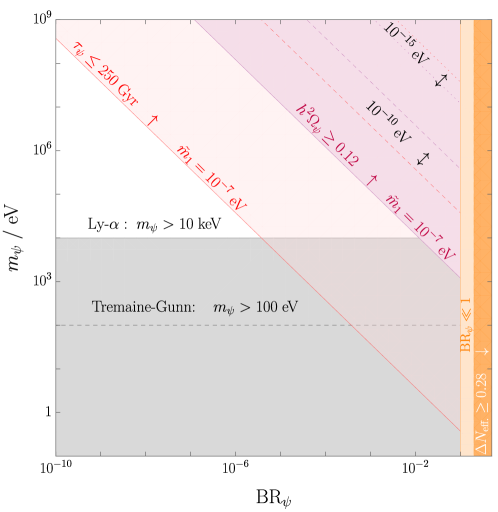
Figure 1: Parameter space for the dark matter mass $m_{\psi}$ versus the branching ratio $\text{BR}_{\psi}$ of the RHN decay to dark matter. Contours with (straight, dashed, dotted) lines correspond to $\tilde{m}_{1}=\left(10^{-7},10^{-10},10^{-15}\right)\;\text{eV}$ . The purple contours reproduce the observed dark matter relic abundance and above the contour the abundance would be too large (for fixed $\tilde{m}_{1}$). The gray regions are excluded because of unsuccessful structure formation (Lyman-$\alpha$) and dark matter not being gravitationally bound (Tremaine-Gunn). On the red contours for the DM lifetime from $\psi\rightarrow\nu_{L}\sigma$ is equal to the observational limit and in the colored region above (for fixed $\tilde{m}_{1}$) the lifetime would be too small. This excludes the lines with $\tilde{m}_{1}=\left(10^{-7},10^{-10}\right)\;\text{eV}$, meaning that here only $\tilde{m}_{1}=10^{-15}\;\text{eV}$ is viable for DM. Note that lifetime bound disappears for $m_{\psi}<m_{\sigma}$, in which case the entire purple region is allowed. The area in light orange is excluded by our assumption $\text{BR}_{\psi}\ll\text{BR}_{L}\simeq 1$ and the orange region would be excluded, if the real scalar also produced in the RHN decay was stable and light enough to be dark radiation (see the discussion below (53)).

Both of these constraints illustrate why we need $\text{BR}_{\psi}\ll\text{BR}_{L}$, which translates to $y_{1}\ll\lambda_{1i}$. In the regime $m_{\sigma}<m_{\psi}$ the following decay from $\nu_{L}-N_{1,2,3}$ mixing after electroweak symmetry breaking becomes kinematically allowed Coy:2021sse and we assume that $m_{\sigma}\ll m_{\psi}$:

$$\Gamma\left(\psi\rightarrow\nu_{L}\sigma\right)=\frac{\left|yy^{\dagger}\right|_{11}}{16\pi}\sum_{i,j}\frac{\lambda_{ji}\lambda^{\dagger}_{ij}\;v^{2}}{M_{j}^{2}}m_{\psi}\simeq\frac{m_{\psi}\;\text{BR}_{\psi}}{8\pi}\frac{\tilde{m}_{1}\sum_{i}m_{i}}{v^{2}}\frac{M_{1}}{M_{2,3}}$$ (47)

Here we summed over the final state lepton flavors, which together with the sum over all three RHNs and making the approximation of factoring out one power of $M_{2,3}$, allows us to trade the $\lambda$-couplings of the active neutrino masses via the Seesaw-relation (5). Equation (43) lets us trade the $y$-couplings for $\text{BR}_{\psi}$ and $\tilde{m}_{1}$ in the limit $\text{BR}_{\psi}\ll\text{BR}_{L}$. Data on baryon acoustic oscillations and structure formation requires a lifetime $\tau_{\psi}=1/\Gamma\left(\psi\rightarrow\nu_{L}\sigma\right)$ for DM decaying to dark radiation of $\tau_{\psi}>(249.6-268.8)\times 10^{9}\;\text{yr}$ Simon:2022ftd depending on the exact dataset used. The resulting bound for $\tau_{\psi}>250\times 10^{9}\;\text{yr}$ reads

$$m_{\psi}\text{BR}_{\psi}<$1.8\text{\times}{10}^{-2}\text{\,}\mathrm{eV}$\cdot\left(\frac{$2\text{\times}{10}^{-7}\text{\,}\mathrm{eV}$}{\tilde{m}_{1}}\right)\cdot\left(\frac{$0.05\text{\,}\mathrm{eV}$}{\sum_{i}m_{i}}\right)\cdot\left(\frac{M_{2,3}/M_{1}}{3}\right)$$ (48)

and is compatible with the relic density (45) for

$$\tilde{m}_{1}<$9.7\text{\times}{10}^{-15}\text{\,}\mathrm{eV}$\cdot\left(\frac{0.12}{\Omega_{\psi}h^{2}}\right)^{2}.$$ (49)

We depict the allowed parameter space in figure 1. Once can see that the parameters $\tilde{m}_{1}=\left(10^{-7},10^{-10}\right)\;\text{eV}$ violate the lifetime constraint, because for each constant $\tilde{m}_{1}$ the purple relic abundance iso-contour line is above the red line for $\tau_{\psi}=250\times 10^{9}\;\text{yr}$. The only viable parameter point in this plot has $\tilde{m}_{1}=10^{-15}\;\text{eV}$ in agreement with (49), because here the lifetime iso-contour is above the line for the relic density and we find dark matter close to the GeV-scale. The previous limits only apply for $m_{\psi}>m_{\sigma}$. In general the scalar $\sigma$ couples to the SM Higgs through the following terms

$$V(H,\sigma)\supset\lambda_{\sigma H}\sigma^{2}\left|H\right|^{2}+\left(\kappa\;\sigma+\text{h.c.}\right)\left|H\right|^{2}.$$ (50)

For $m_{\sigma}>m_{h}$ it could decay to the SM Higgs. If this is kinematically forbidden, there could be decay modes lighter SM fermions such as e.g. the electron $\sigma\rightarrow e^{+}e^{-}e^{+}e^{-}$ via off-shell SM Higgs bosons. In case $\sigma$ has no vev these decays require the $\kappa$ coupling. If $\sigma$ is too light to decay to SM states or the couplings $\lambda_{H\sigma}$ and $\kappa$ are very small, then the relic abundance of $\sigma$ survives until today. In this case and assuming that $\lambda_{H\sigma}$ and $\kappa$ are small enough to avoid thermalization with the SM plasma, the non-thermal $\sigma$ could still exist in the form of dark radiation. Its energy density is found from $n_{\sigma}=n_{\psi}=\text{BR}_{\psi}n_{N}$ to be Mazumdar:2016nzr

$$\rho_{\sigma}(T_{\text{dec.}})=\frac{\pi^{2}}{30}g_{*}(T_{\text{dec.}})\;\text{BR}_{\psi}\;\frac{\sqrt{m_{\sigma}^{2}+\left(\frac{M_{1}}{2}\right)^{2}}}{M_{1}}\;T_{\text{dec.}}^{4}$$ (51)

and we compute the abundance of dark radiation, conventionally parameterized as the number of additional neutrinos as Luo:2020fdt assuming again that $M_{1}\gg m_{\sigma}$:

$$\Delta N_{\text{eff.}} =\frac{4}{7}\cdot g_{*\rho}(T_{\text{dec.}})\cdot\left(\frac{10.75}{g_{*S}(T_{\text{dec.}})}\right)^{\frac{4}{3}}\cdot\frac{\rho_{\sigma}(T_{\text{dec.}})}{\rho_{\text{SM}}(T_{\text{dec.}})}$$ (52)

$$\simeq 0.06\cdot\left(\frac{\text{BR}_{\psi}}{4\%}\right)\cdot\left(\frac{106.75}{g_{*S}(T_{\text{dec.}})}\right)^{\frac{4}{3}}\cdot\left(\frac{g_{*}(T_{\text{dec.}})}{106.75}\right)$$ (53)

We see that $\sigma$ would lead to too much dark radiation compared with the current Planck bound $\Delta N_{\text{eff.}}^{\text{Planck+BAO}}\simeq 0.28$ Planck:2018vyg unless we make the branching ratio $\text{BR}_{\psi}$, which also controls the DM production, smaller than about 20% (see figure 1). However we saw previously that $\text{BR}_{\psi}$ can be far below a percent for heavy enough DM, which is why we do not necessarily expect observable dark radiation. BBN sets a bound of $\Delta N_{\text{eff.}}^{\text{BBN}}\simeq 0.4$ Cyburt:2015mya . The projected sensitivities of upcoming experiments read $\Delta N_{\text{eff}}^{\text{proj.}}=0.014$ for CMB-HD CMB-HD:2022bsz , $\Delta N_{\text{eff}}^{\text{proj.}}=0.05$ for CMB-Bharat CMB-Bharat , $\Delta N_{\text{eff}}^{\text{proj.}}=0.06$ for CMB Stage IV Abazajian:2019eic ; annurev-nucl-102014-021908 and NASA’s PICO mission NASAPICO:2019thw or $\Delta N_{\text{eff.}}\lesssim 0.12$ for CORE CORE:2017oje , the South Pole Telescope SPT-3G:2014dbx as well as the Simons observatory SimonsObservatory:2018koc . Before closing let us emphasize again that $\sigma$ only counts as dark radiation when it is very light and stable or long-lived.

3 Gravitational Waves

3.1 Distortion of the inflationary tensor mode spectrum

We assume primordial inflation ended in an epoch of reheating, creating a Standard Model plasma of radiation with an initial temperature $T_{\text{RH}}$ set by the reheating dynamics. Gravitational waves produced during inflation first leave the horizon and have constant amplitudes while outside the horizon. After they re-enter the horizon the amplitude becomes damped. The power spectrum of gravitational waves (GWs) today can be written as a function of the wave-number $k=2\pi f$ with $f$ being the frequency

$$\Omega_{\text{GW}}(k)=\frac{1}{12}\left(\frac{k}{a_{0}H_{0}}\right)^{2}P_{T}(k),$$ (54)

where $a_{0}=1$ and $H_{0}\simeq$2.2\text{\times}{10}^{-4}\text{\,}{\mathrm{Mpc}}^{-1}$$ Datta:2022tab are the scale factor and expansion rate today and $P_{T}$ denotes the spectrum of tensor modes. It is parameterized in terms of the primordial power spectrum from inflation $P_{T}^{\text{prim.}}$

$$P_{T}(k)=T_{T}^{2}(k)\;P_{T}^{\text{prim.}}(k)$$ (55)

as well as a transfer function $T_{T}^{2}(k)$. This transfer function describes the propagation of GWs $h_{ij}$ in the Friedmann-Lemaitre-Robertson-Walker background

$$h_{ij}^{\prime\prime}+2aHh_{ij}^{\prime}-\Delta h_{ij}=0,$$ (56)

where primes denote derivatives with respect to conformal time, after the horizon re-entry at a temperature of $T_{\text{in}}$ that depends on the wave-number via Nakayama:2008wy

$$T_{\text{in}}=$5.8\text{\times}{10}^{6}\text{\,}\mathrm{GeV}$\cdot\left(\frac{106.75}{g_{*}(T_{\text{in}})}\right)^{\frac{1}{6}}\left(\frac{k}{${10}^{4}\text{\,}{\mathrm{Mpc}}^{-1}$}\right).$$ (57)

The inflationary tensor power spectrum is conventionally parameterized in terms of its amplitude $A_{T}$ and its spectral index $n_{T}$ at the pivot scale $k_{*}=$0.05\text{\,}{\mathrm{Mpc}}^{-1}$$ Planck:2018jri

$$P_{T}^{\text{prim.}}(k)=A_{T}(k_{*})\left(\frac{k}{k_{*}}\right)^{n_{T}}.$$ (58)

This amplitude is related to the scalar power spectrum $P_{\xi}(k_{*})=2.0989\times 10^{-9}$ Planck:2018jri via the tensor-to-scalar-ratio $r<0.035$ BICEP:2021xfz

$$A_{T}(k_{*})=r\;P_{\xi}(k_{*}).$$ (59)

Observations of the cosmic microwave background only constrain the scalar spectral index to be $n_{S}=0.9649\pm 0.0042$ Planck:2018jri , which is why we take $n_{T}$ as a constant free parameter. The case of $n_{T}>0\;(<0)$ is known as a blue-tilted (red-tilted) spectrum. Standard single field slow-roll inflation predicts a red-tilted spectrum, as the tensor spectral index $n_{T}$ satisifes the so-called consistency relation $n_{T}=-r/8$ Liddle:1993fq , however this does not rule out the possibilities of a blue-tilted spectrum, which is well motivated in various scenarios including e.g. string gas cosmology Brandenberger:2006xi , super-inflation models Baldi:2005gk , G-inflation Kobayashi:2010cm , non-commutative inflation Calcagni:2004as ; Calcagni:2013lya , particle production during inflation Cook:2011hg ; Mukohyama:2014gba , and several others Kuroyanagi:2020sfw . Here we will also seek to investigate such scenarios from the perspective of models of the early universe and leptogenesis. An epoch of early or intermediate matter domination would change the transfer function compared to the standard case of radiation domination, and hence the expansion of the background is imprinted in the damping of the gravitational wave amplitude. References Turner:1993vb ; Chongchitnan:2006pe ; Nakayama:2008wy ; Nakayama:2009ce ; Kuroyanagi:2011fy ; Kuroyanagi:2014nba computed this transfer function numerically and found a compact analytical expression with a fitting function $F(k)$

$$T_{T}^{2}(k) =\Omega_{m}^{2}\left(\frac{g_{*}(T_{\text{in}})}{g_{*}^{0}}\right)\left(\frac{g_{*S}^{0}}{g_{*S}(T_{\text{in}})}\right)^{\frac{4}{3}}\left(\frac{3j_{1}(z_{k})}{z_{k}}\right)^{2}F(k)$$ (60)

in terms of the total matter density $\Omega_{m}=0.31$, the first spherical Bessel function $j_{1}(z_{k})$ and $z_{k}\equiv k\;\tau_{0}$ with $\tau_{0}=2/H_{0}$ Datta:2022tab being the conformal time today. The factors of the relativistic degrees of freedom encode the expansion of the universe and we use the fitting functions of reference Kuroyanagi:2014nba for $g_{*}(T_{\text{in}})$ and $g_{*S}(T_{\text{in}})$ with the present day values $g_{*}^{0}=3.36$ and $g_{*S}^{0}=3.91$, whereas the Bessel function describes the damping of the gravitational wave amplitude after horizon re-entry. In the limit $z_{k}\gg 1$, which always holds for the frequencies we are interested in,

$$k\;\tau_{0}\simeq 6\times 10^{15}\left(\frac{f}{10^{-3}\;\text{Hz}}\right),$$ (61)

we can trade the oscillatory $j_{1}(z_{k})$ for $1/(\sqrt{2}z_{k})$. Note that in references Kuroyanagi:2011fy ; Kuroyanagi:2014nba the correct limiting behavior was mentioned for the wrong limit $z_{k}\ll 1$ (for which one would obtain $j_{1}(z_{k})\sim z_{k}$ instead) . We employ the most recent results of Kuroyanagi:2014nba for the fitting function $F(k)$. Without intermediate matter domination it reads

$$F(k)_{\text{standard}}=T_{1}^{2}\left(\frac{k}{k_{\text{eq.}}}\right)T_{2}^{2}\left(\frac{k}{k_{\text{RH}}}\right),$$ (62)

whereas including an epoch of RHN domination leads to

$$F(k)_{\text{IMD}} =T_{1}^{2}\left(\frac{k}{k_{\text{eq.}}}\right)T_{2}^{2}\left(\frac{k}{k_{\text{dec.}}}\right)T_{3}^{2}\left(\frac{k}{k_{\text{dec. S}}}\right)T_{2}^{2}\left(\frac{k}{k_{\text{RH S}}}\right).$$ (63)

Here we introduce

$$k_{\text{eq.}} =$7.1\text{\times}{10}^{-2}\text{\,}{\mathrm{Mpc}}^{-1}$\cdot\Omega_{m}h^{2},$$ (64)

$$k_{\text{dec.}} =$1.7\text{\times}{10}^{14}\text{\,}{\mathrm{Mpc}}^{-1}$\left(\frac{g_{*S}(T_{\text{dec.}})}{g_{*S}^{0}}\right)^{\frac{1}{6}}\left(\frac{T_{\text{dec.}}}{10^{7}\;\text{GeV}}\right),$$ (65)

$$k_{\text{RH}} =$1.7\text{\times}{10}^{14}\text{\,}{\mathrm{Mpc}}^{-1}$\left(\frac{g_{*S}(T_{\text{RH}})}{g_{*S}^{0}}\right)^{\frac{1}{6}}\left(\frac{T_{\text{RH}}}{10^{7}\;\text{GeV}}\right),$$ (66)

$$k_{\text{dec. S}} =k_{\text{dec.}}\Delta^{\frac{2}{3}},$$ (67)

$$k_{\text{RH S}} =k_{\text{RH}}\Delta^{-\frac{1}{3}},$$ (68)

where all quantities with a subscript (superscript) “0” are evaluated today and we set $h=0.7$. The entropy dilution factor $\Delta$ was defined in (27) and the fit functions read

$$T_{1}^{2}(x) =1+1.57x+3.42x^{2},$$ (69)

$$T_{2}^{2}(x) =(1-0.22x^{\frac{3}{2}}+0.65x^{2})^{-1},$$ (70)

$$T_{3}^{2}(x) =1+0.59x+0.65x^{2}.$$ (71)

Physically $T_{1}$ describes the transition from a radiation dominated phase to a matter dominated epoch and $T_{2}$ the case of going from matter domination to radiation domination. $T_{3}$ has the same physical interpretation as $T_{1}$ but allows for a better numerical fit Kuroyanagi:2014nba . One deduces from the wave-number $k_{\text{dec.}}=2\pi f_{\text{sup.}}$ at the time of RHN decay in (65) that the gravitational wave spectrum gets suppressed by the entropy dilution for frequencies above

$$f_{\text{sup.}} \simeq 2.7\times 10^{-10}\;\text{Hz}\;\left(\frac{T_{\text{dec.}}}{$10\text{\,}\mathrm{MeV}$}\right),$$ (72)

$$\simeq 9\times 10^{-2}\;\text{Hz}\cdot\left(\frac{n_{\text{B}}/s}{$8.75\text{\times}{10}^{-11}\text{\,}$}\right)\cdot\left(\frac{$0.05\text{\,}\mathrm{eV}$}{m_{3}-m_{1}}\right)\cdot\left(\frac{106.75}{g_{*}(T_{\text{dec.}})}\right)^{\frac{1}{4}},$$ (73)

where in the last line we fixed $M_{1}$ via equation (34) to reproduce the observed baryon asymmetry, which means that all the RHN decay at $T_{\text{dec.}}=$3.3\text{\times}{10}^{6}\text{\,}\mathrm{GeV}$$ hence the constant $f_{\text{sup.}}$. The suppression factor of the power spectrum is Seto:2003kc

$$R_{\text{sup.}}=\frac{\Omega_{\text{GW}}^{\text{IMD}}}{\Omega_{\text{GW}}^{\text{standard}}}\simeq\frac{1}{\Delta^{\frac{4}{3}}},$$ (74)

which depends only on $\tilde{m_{1}}$ via $\Delta$ in (28). Here $\Omega_{\text{GW}}^{\text{IMD}}$ was computed from (63) and takes the intermediate matter domination (IMD) from the RHN into account, whereas $\Omega_{\text{GW}}^{\text{standard}}$ from (62) appears in the absence of RHN domination.

3.2 Other GW sources

So far, when it comes to gravitational waves, most studies involving the Seesaw mechanism have focused on the dynamics of e.g. the $\text{U}(1)_{\text{B-L}}$ breaking, which underlies the RHN Majorana masses in unified gauge theories Fritzsch:1974nn ; Georgi:1974my . The dynamics of the scalar responsible for breaking this gauge symmetry can source a separate stochastic gravitational wave background by means of a first order Chao:2017ilw ; Okada:2018xdh ; Hasegawa:2019amx ; Haba:2019qol or second order Buchmuller:2013lra ; Buchmuller:2019gfy ; Dror:2019syi phase transition as well as via the formation of a network of cosmic strings PhysRevD.31.3052 ; Dror:2019syi ; Blasi:2020wpy ; Dunsky:2021tih via the Kibble mechanism Kibble:1976sj . If the phase transition or the formation of topological defects happens before inflation - and the symmetry is never (non-)thermally restored - any trace of the B-L transition will be diluted away due to the exponential expansion of space-time. The symmetry is broken throughout inflation and reheating if Redi:2022llj

$$v_{\text{B-L}}>\text{Max}\left[\frac{H_{I}}{2\pi},T_{\text{max.}}\right],$$ (75)

where the first term is the Gibbons-Hawkings temperature PhysRevD152738 in terms of the Hubble rate during inflation $H_{I}$ and the second term the maximum temperature during reheating Garcia:2017tuj ; Garcia:2020eof ; Datta:2022jic , which can be drastically larger than the temperature of the radiation bath at the end of reheating $T_{\text{RH}}$. Since $T_{\text{max.}}$ depends on the reheating scenario, the best we can do to get an estimate on $v_{\text{B-L}}$ is to assume that $H_{I}/(2\pi)>T_{\text{max.}}$ and saturate the current CMB-limit on $H_{I}\lesssim$2.5\text{\times}{10}^{14}\text{\,}\mathrm{GeV}$$ Akrami:2018odb leading to

$$v_{\text{B-L}}\gtrsim$4\text{\times}{10}^{13}\text{\,}\mathrm{GeV}$.$$ (76)

This further motivates why we consider high scale leptogenesis. Moreover this bound is compatible with the condition (24) for a thermalized population of $N_{1}$ from B-L gauge scatterings. Also note that one could even consider a case, where no additional degrees of freedom except the RHN are added to the SM below the Planck scale, so that there would be no source for the stochastic GW background (in this case the initial thermal RHN abundance would have to come from inflaton decays). Consequently our high scale scenario without a stochastic GW background, being essentially independent of the dynamics of the $\text{U}(1)_{\text{B-L}}$ transition and the associated scalar, can be viewed as complementary to the existing analyses.

3.3 Detectors and signal-to-noise ratio

We display the (expected) sensitivity curves for a variety of exisiting and proposed experiments that can be grouped in terms of

• ground based interferometers: LIGO/VIRGO LIGOScientific:2016aoc ; LIGOScientific:2016sjg ; LIGOScientific:2017bnn ; LIGOScientific:2017vox ; LIGOScientific:2017ycc ; LIGOScientific:2017vwq , aLIGO/aVIRGO Harry_2010 ; LIGOScientific:2014pky ; VIRGO:2014yos ; LIGOScientific:2019lzm , AION Badurina:2021rgt ; Graham:2016plp ; Graham:2017pmn ; Badurina:2019hst , Einstein Telescope (ET) Punturo:2010zz ; Hild:2010id , Cosmic Explorer (CE) LIGOScientific:2016wof ; Reitze:2019iox ,

• space based interferometers: LISA 2017arXiv170200786A ; Baker:2019nia , BBO Crowder:2005nr ; Corbin:2005ny ; Harry_2006 , DECIGO, U-DECIGOSeto:2001qf ; Kudoh:2005as ; Kawamura_2006 ; Nakayama:2009ce ; Yagi:2011wg ; Kawamura:2020pcg , AEDGE AEDGE:2019nxb ; Badurina:2021rgt , $\mu$-ARES Sesana:2019vho

• recasts of star surveys: GAIA/THEIA Garcia-Bellido:2021zgu ,

• pulsar timing arrays (PTA): SKA Carilli:2004nx ; Janssen:2014dka ; Weltman:2018zrl , EPTA Kramer_2013 ; Lentati:2015qwp ; Babak:2015lua , NANOGRAV McLaughlin:2013ira ; NANOGRAV:2018hou ; Aggarwal:2018mgp ; Brazier:2019mmu ; NANOGrav:2020bcs

• CMB polarization: Planck 2018 Akrami:2018odb and BICEP 2/ Keck BICEP2:2018kqh computed by Clarke:2020bil , LiteBIRD Hazumi:2019lys ,

• CMB spectral distortions: PIXIE, Super-PIXIE Kogut_2011 ; Kogut:2019vqh , VOYAGER2050 Chluba:2019kpb

Interferometers measure displacements in terms of a so called dimensionless strain-noise $h_{\text{GW}}(f)$ that is related to the GW amplitude and can be converted into the corresponding energy density Garcia-Bellido:2021zgu

$$\Omega_{\text{exp}}(f)h^{2}=\frac{2\pi^{2}f^{2}}{3H_{0}^{2}}h_{\text{GW}}(f)^{2}h^{2},$$ (77)

with $H_{0}=h\times 100\;\text{(km/s)}/\text{Mpc}$ being the Hubble rate today. We compute the signal-to-noise ratio (SNR) for a given or projected experimental sensitivity $\Omega_{\text{exp}}(f)h^{2}$ in order to assess the detection probability of the primordial GW background via the following prescription Thrane:2013oya ; Caprini:2015zlo

$$\text{SNR}\equiv\sqrt{\tau\int_{f_{\text{min}}}^{f_{\text{max}}}\text{d}f\left(\frac{\Omega_{\text{GW}}(f)h^{2}}{\Omega_{\text{exp}}(f)h^{2}}\right)^{2}},$$ (78)

where $h=0.7$ and $\tau=4\;\text{years}$ is the observation time. For this analysis we consider $\text{SNR}\geq 10$ as the detection threshold.

3.4 Dark radiation bounds from BBN and CMB decoupling

The energy density in gravitational waves should be smaller than the limit on dark radiation encoded in $\Delta N_{\text{eff.}}$ from Big Bang Nucleosynthesis and CMB observations (see the discussion below (53) for bounds and projections on $\Delta N_{\text{eff.}}$) Maggiore:1999vm

$$\int_{f_{\text{min}}}^{f=\infty}\frac{\text{d}f}{f}\Omega_{\text{GW}}(f)h^{2}\leq 5.6\times 10^{-6}\;\Delta N_{\text{eff.}}.$$ (79)

The lower limit of the integration is $f_{\text{min}}\simeq 10^{-10}\text{Hz}$ for BBN and $f_{\text{min}}\simeq 10^{-18}\text{Hz}$ for the CMB. In practice, when e.g. plotting many GW spectra simultaneously, and as a first estimate we neglect the frequency dependence to constrain the energy density of the peak for a given spectrum

$$\Omega_{\text{GW}}^{\text{Peak}}h^{2}\leq 5.6\times 10^{-6}\;\Delta N_{\text{eff.}}.$$ (80)

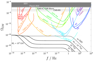
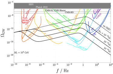
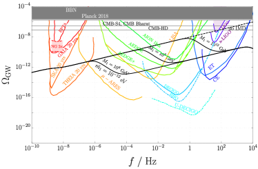
Figure 2: Example GW spectra for $T_{\text{RH}}=10^{8}\;\text{GeV},\;M_{1}=10^{4}\;\text{GeV}$ and $n_{T}=0$ (left) as well as $n_{T}=0.5$ (right). Here we varied $\tilde{m}_{1}=\left(10^{-10},10^{-12},10^{-14}\right)\;\text{eV}$ and “no IMD” refers to the scenario without RHN domination.

Figure 3: Example spectra for $T_{\text{RH}}=10^{12}\;\text{GeV},\;\tilde{m}_{1}=10^{-12}\;\text{eV}$ and $n_{T}=0$ (left) as well as $n_{T}=0.5$ (right). Here we varied $M_{1}=\left(10^{6},10^{9},10^{12}\right)\;\text{GeV}$ and “no IMD” refers to the scenario without RHN domination.

3.5 Impact of free-streaming particles

As shown in the seminal work Weinberg:2003ur and expanded upon in e.g. Watanabe:2006qe ; Stefanek:2012hj ; Dent:2013asa ; Hook:2020phx , there is a damping effect on the GW amplitude from free-streaming particles whose mean free path is larger than the Hubble scale. Free streaming particles such as the active neutrinos, the RHN, additional sources of dark radiation or gravitational waves themselves contribute to anisotropic stress-energy tensor and can reduce the primordial GW amplitude by up to 35.6% Weinberg:2003ur . In this work we neglect this effect to focus on the damping from the RHN induced matter dominated epoch as a first estimate, since percent level effects will only become relevant once we have actual data.

4 Results

4.1 General results

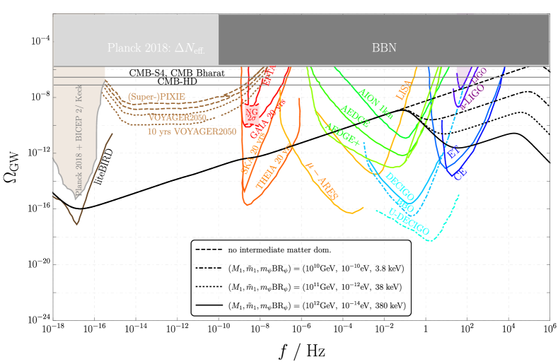
Figure 4: We fix $M_{1}$ as a function of $\tilde{m}_{1}=\left(10^{-10},10^{-12},10^{-14}\right)\;\text{eV}$ for successful leptogenesis and set $T_{\text{RH}}=10^{13}\;\text{GeV},\;n_{T}=0$. Furthermore we show which value of $m_{\psi}\text{BR}_{\psi}$ would be required for a given $\tilde{m}_{1}$ to generate the observed dark matter relic abundance.

Figure 5: We fix $M_{1}$ as a function of $\tilde{m}_{1}=\left(10^{-10},10^{-12},10^{-14}\right)\;\text{eV}$ for successful leptogenesis and set $T_{\text{RH}}=10^{13}\;\text{GeV},\;n_{T}=0.5$. Furthermore we show which value of $m_{\psi}\text{BR}_{\psi}$ would be required for a given $\tilde{m}_{1}$ to generate the observed dark matter relic abundance.

Figure 6: We fix $M_{1}=10^{7}\;\text{GeV},\;\tilde{m}_{1}=10^{-17}\;\text{eV},\;T_{\text{RH}}=5\times 10^{12}\;\text{GeV}$ and $n_{T}=0.85$ to fit the NANOGRAV anomaly NANOGrav:2020bcs . Furthermore we show the value of $m_{\psi}\text{BR}_{\psi}=$12\text{\,}\mathrm{MeV}$$ required for the given $\tilde{m}_{1}$ to generate the observed dark matter relic abundance.

In the following we fix $r=0.035$ BICEP:2021xfz and vary the reheating temperature as well as $M_{1},\tilde{m}_{1}$ together with $n_{T}\geq 0$. We depict some example spectra in figures 3 and 3, where we reproduced the figures from reference Asaka:2020wcr . We depict the constraints from LIGO/VIRGO LIGOScientific:2016aoc ; LIGOScientific:2016sjg ; LIGOScientific:2017bnn ; LIGOScientific:2017vox ; LIGOScientific:2017ycc ; LIGOScientific:2017vwq and NANOGRAV McLaughlin:2013ira ; NANOGRAV:2018hou ; Aggarwal:2018mgp ; Brazier:2019mmu ; NANOGrav:2020bcs observations, the CMB as well as BBN as shaded regions in our plots 3-6. It is important to note that the depicted projection for the sensitivity of U-DECIGO Seto:2001qf ; Kudoh:2005as ; Kawamura_2006 ; Nakayama:2009ce ; Yagi:2011wg ; Kawamura:2020pcg is optimistic, but we do not employ the most optimistic case known as U-DECIGO-corr, which assumes that the noise of the instrument is only given by the irreducible quantum noise Kudoh:2005as and should therefore treated as a hypothetical best case scenario. The proposal for BBO Crowder:2005nr ; Corbin:2005ny ; Harry_2006 is also a bit speculative, because it is supposed to eventually succeed the currently planned LISA mission 2017arXiv170200786A ; Baker:2019nia . To remind the reader of these potential caveats we depict the sensitivities for U-DECIGO and BBO with dashed-dotted lines in the figures 3-6. The plots in figures 5 and 5 depict the case where we fix $M_{1}$ as function of $\tilde{m}_{1}$ according to (34) in order to reproduce the observed baryon asymmetry via leptogenesis. In the aforementioned plot we also depict which values of $m_{\psi}\text{BR}_{\psi}$ would be needed according to (45) to fit the dark matter relic abundance for a given $\tilde{m}_{1}$. The labels “no IMD” in 3, 3 and “no intermediate matter dom.” in 5-5 refer to the scenario without RHN domination computed from (62), where the only dilution arises from inflationary reheating. One can clearly see in 5 and 5 that the primordial tensor modes get diluted by the entropy released in the RHN decay for frequencies above $f_{\text{sup.}}\simeq 0.1\;\text{Hz}$, see (73). Furthermore one can observe in 5-6 that there is second break in the spectra at frequencies larger than $f_{\text{sup.}}\sim T_{\text{dec.}}$. This is due to the inflationary reheating at $T_{\text{RH}}$ and since our scenario is defined by the regime $T_{\text{dec.}}<M_{1}<T_{\text{RH}}$ the second break occurs at a larger frequency. The same figures also show a small subleading suppression of frequencies larger than $\mathcal{O}(10^{-9}\;\text{Hz})$, which is due to the entropy released in the QCD phase transition Hajkarim:2019csy . Irrespective of the value of $n_{T}$, one can deduce from 3-6 that LiteBIRD Hazumi:2019lys will already probe the inflationary tensor modes in the $\left(10^{-16}-10^{-18}\right)\;\text{Hz}$ range. For $n_{T}=0$ we find that U-DECIGO Seto:2001qf ; Kudoh:2005as ; Kawamura_2006 ; Nakayama:2009ce ; Yagi:2011wg ; Kawamura:2020pcg has the best chance to distinguish our entropy suppressed spectra from the standard case without RHN domination depicted by the dashed line in 5. In case neither BBO Crowder:2005nr ; Corbin:2005ny ; Harry_2006 nor U-DECIGO Seto:2001qf ; Kudoh:2005as ; Kawamura_2006 ; Nakayama:2009ce ; Yagi:2011wg ; Kawamura:2020pcg detect the tensor mode background expected from inflation, this does not have to rule out primordial gravitational waves and could be a tell-tale sign of scenarios with entropy dilution, such as ours. In the next section we will analyze this in terms of the SNR. The case of $n_{T}=0.5$ without RHN domination would start to be probed by the dark radiation bounds in (80) from BBN Cyburt:2015mya and Planck Planck:2018vyg (see the dashed line in 5) and is only borderline compatible with the existing LIGO/VIRGO  LIGOScientific:2016aoc ; LIGOScientific:2016sjg ; LIGOScientific:2017bnn ; LIGOScientific:2017vox ; LIGOScientific:2017ycc ; LIGOScientific:2017vwq observations . An attempt to explain the recent anomaly in the 12.5-year dataset NANOGrav:2020bcs of the NANOGRAV collaboration McLaughlin:2013ira ; NANOGRAV:2018hou ; Aggarwal:2018mgp ; Brazier:2019mmu with primordial tensor modes would require an extremely large $n_{T}\simeq 0.85$. The challenge is then to have enough entropy dilution to comply with the dark radiation and LIGO/VIRGO bounds. We depict a spectrum for $M_{1}=10^{7}\;\text{GeV},\;\tilde{m}_{1}=10^{-17}\;\text{eV}$ that could be the source of the anomaly in figure 6 for the case without leptogenesis. The reason for abandoning leptogenesis is simply that with such a large $n_{T}$ the peak of the GW energy density at the typical frequency $f_{\text{sup.}}=$0.1\text{\,}\mathrm{Hz}$$ (before the dilution kicks in) will already be far too large to comply with the dark radiation bounds. Therefore one needs a spectrum where the damping (which is only proportional to $\tilde{m}_{1}$ see (74)) occurs at lower decay temperatures and hence lower frequencies (set by both $M_{1}$ and $\tilde{m}_{1}$ see (14)). This is why we chose a value of $M_{1}=10^{7}\;\text{GeV}$ below the leptogenesis bound in (34). On top of that we set $T_{\text{RH}}=$5\text{\times}{10}^{12}\text{\,}\mathrm{GeV}$$, so that the GWs at large frequencies beyond LIGO/VIRGO do not come into tension with the dark radiation bound due to the damping from inflationary reheating. These estimates illustrate, why we would need a rather contrived scenario and we do not pursue the aforementioned anomaly further in this work.

4.2 Signal-to-noise ratio

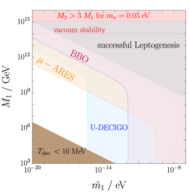
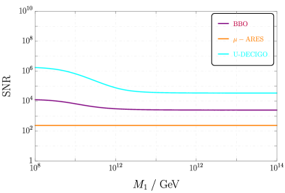
Figure 7: Parameter space in the $M_{1}$ versus $\tilde{m}_{1}$ plane with contours for $\text{SNR}=10$ (left) and SNR as a function of $M_{1}$, where $\tilde{m}_{1}$ was fixed for leptogenesis via (34) (right). In both plots we fixed $T_{\text{RH}}=10^{16}\;\text{GeV},\;n_{T}=0$. See the main text for details on the constraints. The SNR is larger than 10 in the colored regions. Note that the colored lines from the experiments do no correspond to constraints, but to projections of future sensitivities.

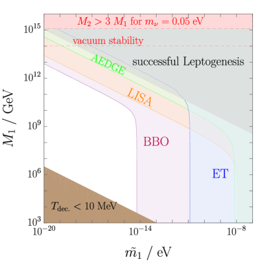
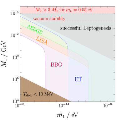
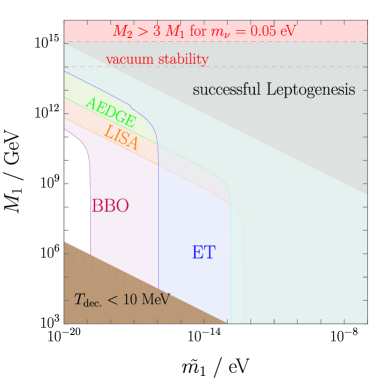
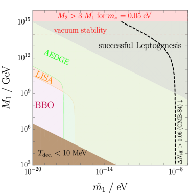
Figure 8: Parameter space in the $M_{1}$ versus $\tilde{m}_{1}$ plane with contours for $\text{SNR}=10$ for $n_{T}=0.1$ (left) and $n_{T}=0.2$ (right). In both plots we fixed $T_{\text{RH}}=10^{16}\;\text{GeV}$. See the main text for details on the constraints. The SNR is larger than 10 in the colored regions. Note that the colored lines from the experiments do no correspond to constraints, but to projections of future sensitivities.

Figure 9: Parameter space in the $M_{1}$ versus $\tilde{m}_{1}$ plane with contours for $\text{SNR}=10$ for $n_{T}=0.3$ (left) and $n_{T}=0.5$ (right). In both plots we fixed $T_{\text{RH}}=10^{16}\;\text{GeV}$. See the main text for details on the constraints. The SNR is larger than 10 in the colored regions. Note that the colored lines from the experiments do no correspond to constraints, but to projections of future sensitivities.

We use the SNR defined in (78) to determine the region in the $M_{1}$ versus $\tilde{m}_{1}$ parameter space, where a detection of primordial gravitational waves can be claimed for a SNR threshold of ten over four years of observation time. For $n_{T}=0$ we find that BBO Crowder:2005nr ; Corbin:2005ny ; Harry_2006 , $\mu$-ARES Sesana:2019vho and U-DECIGO Seto:2001qf ; Kudoh:2005as ; Kawamura_2006 ; Nakayama:2009ce ; Yagi:2011wg ; Kawamura:2020pcg are the most relevant experiments that have a chance of probing the primordial GW background, as can be deduced from figure 5. For $n_{T}>0$ there are a lot more experiments that can probe our GW spectra, which is why we focus on AEDGE AEDGE:2019nxb ; Badurina:2021rgt , BBO Crowder:2005nr ; Corbin:2005ny ; Harry_2006 , the Einstein Telescope (ET) Punturo:2010zz ; Hild:2010id and LISA 2017arXiv170200786A ; Baker:2019nia . Of course there are also other currently developed experiments, such as the radio telescope SKA Carilli:2004nx ; Janssen:2014dka ; Weltman:2018zrl , that become relevant for $n_{T}>0$. The parameter space for $n_{T}=0$ was displayed in 7, whereas figure 9 showcases $n_{T}=0.1,\;0.2$ and 9 the cases of $n_{T}=0.3,\;0.5$. The region in (34) that leads to the observed baryon asymmetry via leptogenesis was shaded in gray. For $n_{T}=0.1$ one can conclude from the left plot in figure 9 that the SNR threshold for ET Punturo:2010zz ; Hild:2010id will start to probe the edge of the parameter space for leptogenesis in the regime $\tilde{m}_{1}\lesssim 10^{-11}\;\text{eV}$. For $n_{T}>0$ we see in 9-9 that AEDGE AEDGE:2019nxb ; Badurina:2021rgt , BBO  Crowder:2005nr ; Corbin:2005ny ; Harry_2006 and LISA  2017arXiv170200786A ; Baker:2019nia probe the entire parameter space for leptogenesis. We impose the following constraints in figures 7-9: Successful BBN requires that the RHN decay temperature in (14) is at least $10\;\text{MeV}$ Kawasaki:2000en ; Hannestad:2004px , which was depicted as a brown region. RHN with masses above $10^{14}\;\text{GeV}$ could destabilize the electroweak vacuum Casas:1999cd ; Elias-Miro:2011sqh . We do not show the bound $M_{1}\lesssim 10^{7}\;\text{GeV}$ Vissani:1997ys ; Clarke:2015gwa ; Brivio:2017dfq ; Brivio:2018rzm from the naturalness of the Higgs mass under corrections from its couplings to the RHN, as it would basically exclude our entire parameter space in (34). The last bound comes from the observed neutrino masses: Due to the perturbativity of the RHN Yukawa coupling $\lambda_{ij}<\sqrt{4\pi}$ and the need to reproduce at least one mass eigenstate with $m_{\nu}=$0.05\text{\,}\mathrm{eV}$$ we find that $M_{2}\lesssim$3.8\text{\times}{10}^{15}\text{\,}\mathrm{GeV}$$. This together with our assumption that $M_{2}>3M_{1}$ means that we have to require at least $M_{1}\lesssim 10^{15}\;\text{GeV}$. In all plots we fixed $T_{\text{RH}}=10^{16}\;\text{GeV}$ so that even the heaviest $N_{1}$ allowed by the previous considerations would be present in the plasma. As mentioned in the previous section we find that U-DECIGO Seto:2001qf ; Kudoh:2005as ; Kawamura_2006 ; Nakayama:2009ce ; Yagi:2011wg ; Kawamura:2020pcg is the best candidate to test our setup compared to the case with no decaying RHN for $n_{T}=0$. A future non-observation of the inflationary tensor mode spectrum could be explained by a decaying $N_{1}$ with $\tilde{m}_{1}<10^{-14}\;\text{eV}$ and a mass of $M_{1}\gtrsim 10^{4}\;\text{GeV}$ (the precise number depends on the BBN bound on the RHN decay temperature of at least $10\;\text{MeV}$). By fixing $\tilde{m}_{1}$ as a function of $M_{1}$ for leptogenesis via (34) we plot the SNR as a function of $M_{1}$ on the right side of 7. Here the SNR for $\mu$-ARES Sesana:2019vho is constant because the peak of its sensitivity is situated at a frequency below $f_{\text{sup.}}\simeq 0.1\;\text{Hz}$ and it is therefore blind to the entropy damping. For cosmologies with $n_{T}>0$ we find that the SNR for U-DECIGO Seto:2001qf ; Kudoh:2005as ; Kawamura_2006 ; Nakayama:2009ce ; Yagi:2011wg ; Kawamura:2020pcg is always larger than 10 in the depicted parameter space, which is why we focus on different detectors. BBO Crowder:2005nr ; Corbin:2005ny ; Harry_2006 is a promising candidate for a detection of primordial GWs with both $n_{T}=0$ and $n_{T}>0$ (compare the plots in 7 and 9, 9). For $n_{T}\gtrsim 0.5$ the dark radiation bound becomes important again and we show the contour $\Delta N_{\text{eff}}^{\text{proj.}}=0.06$ for CMB Stage IV Abazajian:2019eic ; annurev-nucl-102014-021908 computed via (79) on the right side of figure 9. For completeness we display the SNR as a function of $M_{1}$ (with $\tilde{m}_{1}$ fixed by leptogenesis (34)) for $n_{T}=0.1,\;0.5$ in figure 10.

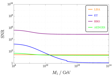
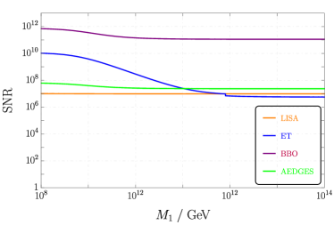
Figure 10: SNR as a function of $M_{1}$, where $\tilde{m}_{1}$ was fixed for leptogenesis via (34) with $n_{T}=0.1$ (left) and $n_{T}=0.5$ (right). In both plots we fixed $T_{\text{RH}}=10^{16}\;\text{GeV}$

5 Conclusions and Discussions

We focused on the minimal Seesaw model, which adds only three right handed neutrinos (RHN) to the SM, and demonstrated that an epoch of right handed neutrino domination, with a Yukawa coupling corresponding to $\tilde{m}_{1}<$2.9\text{\times}{10}^{-7}\text{\,}\mathrm{eV}$$, can realize baryogenesis via leptogenesis for a mass of $M_{1}\gtrsim$2.4\text{\times}{10}^{8}\text{\,}\mathrm{GeV}$\cdot\sqrt{$2\text{\times}{10}^{-7}\text{\,}\mathrm{eV}$/\tilde{m}_{1}}$ (see (34)). Since the effective mass is $\tilde{m}_{1}$ is too small for a thermal RHN population, we had to assume a different production channel via either inflaton decays or B-L gauge scatterings for the initial RHN abundance. Furthermore such a small $\tilde{m}_{1}$ requires that one of the SM neutrinos is approximately massless compared to the other two. The amplitude of gravitational waves that re-enter the horizon before the end of the RHN matter dominated epoch is damped by a factor proportional to the entropy released in the RHN decay. We discussed the detection possibilities of primordial GWs and computed the signal-to-noise ratio for various detectors such as AEDGE AEDGE:2019nxb ; Badurina:2021rgt , BBO Crowder:2005nr ; Corbin:2005ny ; Harry_2006 , DECIGO Seto:2001qf ; Kudoh:2005as ; Kawamura_2006 ; Nakayama:2009ce ; Yagi:2011wg ; Kawamura:2020pcg , Einstein Telescope Punturo:2010zz ; Hild:2010id , LISA 2017arXiv170200786A ; Baker:2019nia or $\mu$-ARES Sesana:2019vho as well as for several spectral tilts $n_{T}\geq 0$ of the tensor mode spectrum. Additionally we determined the regions in the $M_{1}$ versus $\tilde{m}_{1}$ parameter space in which the signal-to-noise ratio (SNR) is larger than ten over a four year observational period in the figures 7-9. Our main finding is that high scale leptogenesis can have an observable imprint on the gravitational waves from inflation. Further we discussed under which conditions our scenario leads to the dominant GW signal. Since fixing $M_{1}$ as a function of $\tilde{m}_{1}$ for successful leptogenesis by saturating the maximum of the CP-violating decay parameter $\varepsilon_{1}$ for a hierarchical spectrum (see (30)) completely determines the RHN decay temperature to be $T_{\text{dec.}}\simeq$3.3\text{\times}{10}^{6}\text{\,}\mathrm{GeV}$$, we find a constant characteristic frequency of $f_{\text{sup.}}\simeq$0.1\text{\,}\mathrm{Hz}$$ (see (73) and figures 5-5), above which the suppression of the GW amplitude manifests itself. The same RHN can also have a second potentially suppressed decay mode to a stable fermion $\psi$, that is responsible for the dark matter abundance, if the product of the DM mass and the branching fraction of the RHN decay to DM satisfies $m_{\psi}\text{BR}_{\psi}\simeq$85\text{\,}\mathrm{eV}$\cdot\sqrt{$2\text{\times}{10}^{-7}\text{\,}\mathrm{eV}$/\tilde{m}_{1}}$. In order for the dark matter do be heavy enough for successful structure formation ($m_{\psi}>\mathcal{O}($10\text{\,}\mathrm{keV}$)$) for fixed $\tilde{m}_{1}$ we typically need a small branching ratio $\text{BR}_{\psi}\ll 1$. Such a small branching fraction can also suppress the amount of BSM dark radiation $\Delta N_{\text{eff.}}\simeq 0.06\cdot(\text{BR}_{\psi}/4\%)$, that could potentially be generated, if the scalar produced together with $\psi$ is very light and survives until today. This particular scenario leads to GeV-scale DM decaying to dark radiation and SM neutrinos, which necessitates $\tilde{m}_{1}<$9.7\text{\times}{10}^{-15}\text{\,}\mathrm{eV}$$ in order to have DM with a large enough lifetime on cosmological scales and the right relic abundance.

References

- (1) Y. Fukuda, T. Hayakawa, K. Inoue, K. Ishihara, H. Ishino, S. Joukou et al., Solar neutrino data covering solar cycle 22, Physical Review Letters 77 (1996) 1683.
- (2) Super-Kamiokande collaboration, Constraints on neutrino oscillations using 1258 days of Super-Kamiokande solar neutrino data, Phys. Rev. Lett. 86 (2001) 5656 [hep-ex/0103033].
- (3) Super-Kamiokande collaboration, Determination of solar neutrino oscillation parameters using 1496 days of Super-Kamiokande I data, Phys. Lett. B 539 (2002) 179 [hep-ex/0205075].
- (4) SNO collaboration, Direct evidence for neutrino flavor transformation from neutral current interactions in the Sudbury Neutrino Observatory, Phys. Rev. Lett. 89 (2002) 011301 [nucl-ex/0204008].
- (5) Super-Kamiokande collaboration, A Measurement of atmospheric neutrino oscillation parameters by SUPER-KAMIOKANDE I, Phys. Rev. D 71 (2005) 112005 [hep-ex/0501064].
- (6) B. Aharmim, S. Ahmed, J. Amsbaugh, J. Anaya, A. Anthony, J. Banar et al., Measurement of the and total 8b solar neutrino fluxes with the sudbury neutrino observatory phase-iii data set, Physical Review C 87 (2011) .
- (7) Super-Kamiokande Collaboration collaboration, Solar neutrino measurements in super-kamiokande-iv, Phys. Rev. D 94 (2016) 052010.
- (8) Borexino collaboration, Measurement of neutrino flux from the primary proton–proton fusion process in the Sun with Borexino detector, Phys. Part. Nucl. 47 (2016) 995 [1507.02432].
- (9) IceCube collaboration, Measurement of Atmospheric Neutrino Oscillations at 6–56 GeV with IceCube DeepCore, Phys. Rev. Lett. 120 (2018) 071801 [1707.07081].
- (10) ANTARES collaboration, Measuring the atmospheric neutrino oscillation parameters and constraining the 3+1 neutrino model with ten years of ANTARES data, JHEP 06 (2019) 113 [1812.08650].
- (11) KamLAND collaboration, Precision Measurement of Neutrino Oscillation Parameters with KamLAND, Phys. Rev. Lett. 100 (2008) 221803 [0801.4589].
- (12) T2K collaboration, Indication of Electron Neutrino Appearance from an Accelerator-produced Off-axis Muon Neutrino Beam, Phys. Rev. Lett. 107 (2011) 041801 [1106.2822].
- (13) Double Chooz collaboration, Indication of Reactor Disappearance in the Double Chooz Experiment, Phys. Rev. Lett. 108 (2012) 131801 [1112.6353].
- (14) T2K collaboration, Observation of Electron Neutrino Appearance in a Muon Neutrino Beam, Phys. Rev. Lett. 112 (2014) 061802 [1311.4750].
- (15) KATRIN collaboration, Direct neutrino-mass measurement with sub-electronvolt sensitivity, Nature Phys. 18 (2022) 160 [2105.08533].
- (16) Planck collaboration, Planck 2018 results. VI. Cosmological parameters, Astron. Astrophys. 641 (2020) A6 [1807.06209].
- (17) eBOSS collaboration, Completed SDSS-IV extended Baryon Oscillation Spectroscopic Survey: Cosmological implications from two decades of spectroscopic surveys at the Apache Point Observatory, Phys. Rev. D 103 (2021) 083533 [2007.08991].
- (18) J. Martin, C. Ringeval and V. Vennin, Encyclopædia Inflationaris, Phys. Dark Univ. 5-6 (2014) 75 [1303.3787].
- (19) L.P. Grishchuk, Amplification of gravitational waves in an istropic universe, Zh. Eksp. Teor. Fiz. 67 (1974) 825.
- (20) A.A. Starobinsky, Spectrum of relict gravitational radiation and the early state of the universe, JETP Lett. 30 (1979) 682.
- (21) V.A. Rubakov, M.V. Sazhin and A.V. Veryaskin, Graviton Creation in the Inflationary Universe and the Grand Unification Scale, Phys. Lett. B 115 (1982) 189.
- (22) M.C. Guzzetti, N. Bartolo, M. Liguori and S. Matarrese, Gravitational waves from inflation, Riv. Nuovo Cim. 39 (2016) 399 [1605.01615].
- (23) N. Seto and J. Yokoyama, Probing the equation of state of the early universe with a space laser interferometer, J. Phys. Soc. Jap. 72 (2003) 3082 [gr-qc/0305096].
- (24) L.A. Boyle and P.J. Steinhardt, Probing the early universe with inflationary gravitational waves, Phys. Rev. D 77 (2008) 063504 [astro-ph/0512014].
- (25) L.A. Boyle and A. Buonanno, Relating gravitational wave constraints from primordial nucleosynthesis, pulsar timing, laser interferometers, and the CMB: Implications for the early Universe, Phys. Rev. D 78 (2008) 043531 [0708.2279].
- (26) S. Kuroyanagi, T. Chiba and N. Sugiyama, Precision calculations of the gravitational wave background spectrum from inflation, Phys. Rev. D 79 (2009) 103501 [0804.3249].
- (27) K. Nakayama and J. Yokoyama, Gravitational Wave Background and Non-Gaussianity as a Probe of the Curvaton Scenario, JCAP 01 (2010) 010 [0910.0715].
- (28) S. Kuroyanagi, C. Ringeval and T. Takahashi, Early universe tomography with CMB and gravitational waves, Phys. Rev. D 87 (2013) 083502 [1301.1778].
- (29) R. Jinno, T. Moroi and K. Nakayama, Inflationary Gravitational Waves and the Evolution of the Early Universe, JCAP 01 (2014) 040 [1307.3010].
- (30) K. Saikawa and S. Shirai, Primordial gravitational waves, precisely: The role of thermodynamics in the Standard Model, JCAP 05 (2018) 035 [1803.01038].
- (31) N. Bernal, A. Ghoshal, F. Hajkarim and G. Lambiase, Primordial Gravitational Wave Signals in Modified Cosmologies, JCAP 11 (2020) 051 [2008.04959].
- (32) K. Nakayama, S. Saito, Y. Suwa and J. Yokoyama, Space laser interferometers can determine the thermal history of the early Universe, Phys. Rev. D 77 (2008) 124001 [0802.2452].
- (33) K. Nakayama, S. Saito, Y. Suwa and J. Yokoyama, Probing reheating temperature of the universe with gravitational wave background, JCAP 06 (2008) 020 [0804.1827].
- (34) S. Kuroyanagi, K. Nakayama and S. Saito, Prospects for determination of thermal history after inflation with future gravitational wave detectors, Phys. Rev. D 84 (2011) 123513 [1110.4169].
- (35) W. Buchmüller, V. Domcke, K. Kamada and K. Schmitz, The Gravitational Wave Spectrum from Cosmological Breaking, JCAP 10 (2013) 003 [1305.3392].
- (36) W. Buchmuller, V. Domcke, K. Kamada and K. Schmitz, A Minimal Supersymmetric Model of Particle Physics and the Early Universe, 1309.7788.
- (37) R. Jinno, T. Moroi and T. Takahashi, Studying Inflation with Future Space-Based Gravitational Wave Detectors, JCAP 12 (2014) 006 [1406.1666].
- (38) S. Kuroyanagi, K. Nakayama and J. Yokoyama, Prospects of determination of reheating temperature after inflation by DECIGO, PTEP 2015 (2015) 013E02 [1410.6618].
- (39) S. Schettler, T. Boeckel and J. Schaffner-Bielich, Imprints of the QCD Phase Transition on the Spectrum of Gravitational Waves, Phys. Rev. D 83 (2011) 064030 [1010.4857].
- (40) F. Hajkarim, J. Schaffner-Bielich, S. Wystub and M.M. Wygas, Effects of the QCD Equation of State and Lepton Asymmetry on Primordial Gravitational Waves, Phys. Rev. D 99 (2019) 103527 [1904.01046].
- (41) R. Jinno, T. Moroi and K. Nakayama, Probing dark radiation with inflationary gravitational waves, Phys. Rev. D 86 (2012) 123502 [1208.0184].
- (42) R.R. Caldwell, T.L. Smith and D.G.E. Walker, Using a Primordial Gravitational Wave Background to Illuminate New Physics, Phys. Rev. D 100 (2019) 043513 [1812.07577].
- (43) Particle Data Group collaboration, Review of Particle Physics, PTEP 2020 (2020) 083C01.
- (44) B.D. Fields, K.A. Olive, T.-H. Yeh and C. Young, Big-Bang Nucleosynthesis after Planck, JCAP 03 (2020) 010 [1912.01132].
- (45) F. Zwicky, Die Rotverschiebung von extragalaktischen Nebeln, Helv. Phys. Acta 6 (1933) 110.
- (46) V.C. Rubin and W.K. Ford, Jr., Rotation of the Andromeda Nebula from a Spectroscopic Survey of Emission Regions, Astrophys. J. 159 (1970) 379.
- (47) D. Clowe, M. Bradac, A.H. Gonzalez, M. Markevitch, S.W. Randall, C. Jones et al., A direct empirical proof of the existence of dark matter, Astrophys. J. Lett. 648 (2006) L109 [astro-ph/0608407].
- (48) A.D. Sakharov, Violation of CP Invariance, C asymmetry, and baryon asymmetry of the universe, Pisma Zh. Eksp. Teor. Fiz. 5 (1967) 32.
- (49) P. Minkowski, at a Rate of One Out of Muon Decays?, Phys. Lett. B 67 (1977) 421.
- (50) T. Yanagida, Horizontal gauge symmetry and masses of neutrinos, Conf. Proc. C 7902131 (1979) 95.
- (51) M. Gell-Mann, P. Ramond and R. Slansky, Complex Spinors and Unified Theories, Conf. Proc. C 790927 (1979) 315 [1306.4669].
- (52) S.L. Glashow, The Future of Elementary Particle Physics, NATO Sci. Ser. B 61 (1980) 687.
- (53) T. Yanagida, Horizontal Symmetry and Masses of Neutrinos, Progress of Theoretical Physics 64 (1980) 1103 [https://academic.oup.com/ptp/article-pdf/64/3/1103/5394376/64-3-1103.pdf].
- (54) R.N. Mohapatra and G. Senjanović, Neutrino mass and spontaneous parity nonconservation, Phys. Rev. Lett. 44 (1980) 912.
- (55) M. Fukugita and T. Yanagida, Baryogenesis Without Grand Unification, Phys. Lett. B 174 (1986) 45.
- (56) M.A. Luty, Baryogenesis via leptogenesis, Phys. Rev. D 45 (1992) 455.
- (57) M. Plumacher, Baryogenesis and lepton number violation, Z. Phys. C 74 (1997) 549 [hep-ph/9604229].
- (58) L. Covi, E. Roulet and F. Vissani, CP violating decays in leptogenesis scenarios, Phys. Lett. B 384 (1996) 169 [hep-ph/9605319].
- (59) G.F. Giudice, A. Notari, M. Raidal, A. Riotto and A. Strumia, Towards a complete theory of thermal leptogenesis in the SM and MSSM, Nucl. Phys. B 685 (2004) 89 [hep-ph/0310123].
- (60) V.A. Kuzmin, V.A. Rubakov and M.E. Shaposhnikov, On the Anomalous Electroweak Baryon Number Nonconservation in the Early Universe, Phys. Lett. B 155 (1985) 36.
- (61) E.W. Kolb and M.S. Turner, The Early Universe, vol. 69, Westview Press (1990), 10.1201/9780429492860.
- (62) G. Arcadi, M. Dutra, P. Ghosh, M. Lindner, Y. Mambrini, M. Pierre et al., The waning of the WIMP? A review of models, searches, and constraints, Eur. Phys. J. C 78 (2018) 203 [1703.07364].
- (63) J.L. Feng, A. Rajaraman and F. Takayama, Superweakly interacting massive particles, Phys. Rev. Lett. 91 (2003) 011302 [hep-ph/0302215].
- (64) L.J. Hall, K. Jedamzik, J. March-Russell and S.M. West, Freeze-In Production of FIMP Dark Matter, JHEP 03 (2010) 080 [0911.1120].
- (65) N. Bernal, M. Heikinheimo, T. Tenkanen, K. Tuominen and V. Vaskonen, The Dawn of FIMP Dark Matter: A Review of Models and Constraints, Int. J. Mod. Phys. A 32 (2017) 1730023 [1706.07442].
- (66) G.B. Gelmini and P. Gondolo, Neutralino with the right cold dark matter abundance in (almost) any supersymmetric model, Phys. Rev. D 74 (2006) 023510 [hep-ph/0602230].
- (67) A. Falkowski, J.T. Ruderman and T. Volansky, Asymmetric Dark Matter from Leptogenesis, JHEP 05 (2011) 106 [1101.4936].
- (68) A. Falkowski, E. Kuflik, N. Levi and T. Volansky, Light Dark Matter from Leptogenesis, Phys. Rev. D 99 (2019) 015022 [1712.07652].
- (69) R.J. Scherrer and M.S. Turner, Decaying particles do not “heat up” the universe, Phys. Rev. D 31 (1985) 681.
- (70) F. Bezrukov, H. Hettmansperger and M. Lindner, keV sterile neutrino Dark Matter in gauge extensions of the Standard Model, Phys. Rev. D 81 (2010) 085032 [0912.4415].
- (71) W. Buchmuller, P. Di Bari and M. Plumacher, Leptogenesis for pedestrians, Annals Phys. 315 (2005) 305 [hep-ph/0401240].
- (72) A. Pilaftsis and T.E.J. Underwood, Resonant leptogenesis, Nucl. Phys. B 692 (2004) 303 [hep-ph/0309342].
- (73) K. Moffat, S. Pascoli, S.T. Petcov, H. Schulz and J. Turner, Three-flavored nonresonant leptogenesis at intermediate scales, Phys. Rev. D 98 (2018) 015036 [1804.05066].
- (74) J. Schechter and J.W.F. Valle, Neutrinoless Double beta Decay in SU(2) x U(1) Theories, Phys. Rev. D 25 (1982) 2951.
- (75) S. Dell’Oro, S. Marcocci, M. Viel and F. Vissani, Neutrinoless double beta decay: 2015 review, Adv. High Energy Phys. 2016 (2016) 2162659 [1601.07512].
- (76) R.E. Shrock, New Tests For, and Bounds On, Neutrino Masses and Lepton Mixing, Phys. Lett. B 96 (1980) 159.
- (77) B. Kayser and R.E. Shrock, Distinguishing Between Dirac and Majorana Neutrinos in Neutral Current Reactions, Phys. Lett. B 112 (1982) 137.
- (78) J. De Vries, H.K. Dreiner, J.Y. Günther, Z.S. Wang and G. Zhou, Long-lived Sterile Neutrinos at the LHC in Effective Field Theory, JHEP 03 (2021) 148 [2010.07305].
- (79) T. Endoh, S. Kaneko, S.K. Kang, T. Morozumi and M. Tanimoto, CP violation in neutrino oscillation and leptogenesis, Phys. Rev. Lett. 89 (2002) 231601 [hep-ph/0209020].
- (80) I. Esteban, M.C. Gonzalez-Garcia, M. Maltoni, I. Martinez-Soler and T. Schwetz, Updated fit to three neutrino mixing: exploring the accelerator-reactor complementarity, JHEP 01 (2017) 087 [1611.01514].
- (81) E. Bertuzzo, P. Di Bari and L. Marzola, The problem of the initial conditions in flavoured leptogenesis and the tauon -dominated scenario, Nucl. Phys. B 849 (2011) 521 [1007.1641].
- (82) S. Ipek, A.D. Plascencia and J. Turner, Assessing Perturbativity and Vacuum Stability in High-Scale Leptogenesis, JHEP 12 (2018) 111 [1806.00460].
- (83) D. Croon, N. Fernandez, D. McKeen and G. White, Stability, reheating and leptogenesis, JHEP 06 (2019) 098 [1903.08658].
- (84) J.A. Dror, T. Hiramatsu, K. Kohri, H. Murayama and G. White, Testing the Seesaw Mechanism and Leptogenesis with Gravitational Waves, Phys. Rev. Lett. 124 (2020) 041804 [1908.03227].
- (85) B. Barman, D. Borah, A. Dasgupta and A. Ghoshal, Probing high scale Dirac leptogenesis via gravitational waves from domain walls, Phys. Rev. D 106 (2022) 015007 [2205.03422].
- (86) D.I. Dunsky, A. Ghoshal, H. Murayama, Y. Sakakihara and G. White, GUTs, hybrid topological defects, and gravitational waves, Phys. Rev. D 106 (2022) 075030 [2111.08750].
- (87) A. Dasgupta, P.S.B. Dev, A. Ghoshal and A. Mazumdar, Gravitational wave pathway to testable leptogenesis, Phys. Rev. D 106 (2022) 075027 [2206.07032].
- (88) D. Borah, A. Dasgupta and I. Saha, Leptogenesis and dark matter through relativistic bubble walls with observable gravitational waves, JHEP 11 (2022) 136 [2207.14226].
- (89) A. Ghoshal, R. Samanta and G. White, Bremsstrahlung High-frequency Gravitational Wave Signatures of High-scale Non-thermal Leptogenesis, 2211.10433.
- (90) N. Bhaumik, A. Ghoshal and M. Lewicki, Doubly peaked induced stochastic gravitational wave background: testing baryogenesis from primordial black holes, JHEP 07 (2022) 130 [2205.06260].
- (91) N. Bhaumik, A. Ghoshal, R.K. Jain and M. Lewicki, Distinct signatures of spinning PBH domination and evaporation: doubly peaked gravitational waves, dark relics and CMB complementarity, 2212.00775.
- (92) T. Vachaspati and A. Vilenkin, Gravitational radiation from cosmic strings, Phys. Rev. D 31 (1985) 3052.
- (93) W. Chao, W.-F. Cui, H.-K. Guo and J. Shu, Gravitational wave imprint of new symmetry breaking, Chin. Phys. C 44 (2020) 123102 [1707.09759].
- (94) N. Okada and O. Seto, Probing the seesaw scale with gravitational waves, Phys. Rev. D 98 (2018) 063532 [1807.00336].
- (95) W. Buchmuller, V. Domcke, H. Murayama and K. Schmitz, Probing the scale of grand unification with gravitational waves, Phys. Lett. B 809 (2020) 135764 [1912.03695].
- (96) T. Hasegawa, N. Okada and O. Seto, Gravitational waves from the minimal gauged model, Phys. Rev. D 99 (2019) 095039 [1904.03020].
- (97) N. Haba and T. Yamada, Gravitational waves from phase transition in minimal SUSY model, Phys. Rev. D 101 (2020) 075027 [1911.01292].
- (98) S. Blasi, V. Brdar and K. Schmitz, Fingerprint of low-scale leptogenesis in the primordial gravitational-wave spectrum, Phys. Rev. Res. 2 (2020) 043321 [2004.02889].
- (99) J.A. Casas and A. Ibarra, Oscillating neutrinos and , Nucl. Phys. B 618 (2001) 171 [hep-ph/0103065].
- (100) E.W. Kolb and S. Wolfram, Baryon Number Generation in the Early Universe, Nucl. Phys. B 172 (1980) 224.
- (101) M. Fujii, K. Hamaguchi and T. Yanagida, Leptogenesis with almost degenerate majorana neutrinos, Phys. Rev. D 65 (2002) 115012 [hep-ph/0202210].
- (102) G.F. Giudice, M. Peloso, A. Riotto and I. Tkachev, Production of massive fermions at preheating and leptogenesis, JHEP 08 (1999) 014 [hep-ph/9905242].
- (103) Particle Data Group collaboration, Review of Particle Physics, PTEP 2022 (2022) 083C01.
- (104) I. Esteban, M.C. Gonzalez-Garcia, M. Maltoni, T. Schwetz and A. Zhou, The fate of hints: updated global analysis of three-flavor neutrino oscillations, JHEP 09 (2020) 178 [2007.14792].
- (105) Super-Kamiokande collaboration, Solar neutrino measurements in super-Kamiokande-I, Phys. Rev. D 73 (2006) 112001 [hep-ex/0508053].
- (106) Super-Kamiokande collaboration, Evidence for an oscillatory signature in atmospheric neutrino oscillation, Phys. Rev. Lett. 93 (2004) 101801 [hep-ex/0404034].
- (107) F. Hahn-Woernle and M. Plumacher, Effects of reheating on leptogenesis, Nucl. Phys. B 806 (2009) 68 [0801.3972].
- (108) H. Fritzsch and P. Minkowski, Unified Interactions of Leptons and Hadrons, Annals Phys. 93 (1975) 193.
- (109) H. Georgi, The State of the Art—Gauge Theories, AIP Conf. Proc. 23 (1975) 575.
- (110) M.A.G. Garcia, Y. Mambrini, K.A. Olive and M. Peloso, Enhancement of the Dark Matter Abundance Before Reheating: Applications to Gravitino Dark Matter, Phys. Rev. D 96 (2017) 103510 [1709.01549].
- (111) M.A.G. Garcia, K. Kaneta, Y. Mambrini and K.A. Olive, Reheating and Post-inflationary Production of Dark Matter, Phys. Rev. D 101 (2020) 123507 [2004.08404].
- (112) A. Datta, R. Roshan and A. Sil, Effects of Reheating on Charged Lepton Yukawa Equilibration and Leptogenesis, 2206.10650.
- (113) G. Engelhard, Y. Grossman, E. Nardi and Y. Nir, The Importance of N2 leptogenesis, Phys. Rev. Lett. 99 (2007) 081802 [hep-ph/0612187].
- (114) J.A. Harvey and M.S. Turner, Cosmological baryon and lepton number in the presence of electroweak fermion-number violation, Phys. Rev. D 42 (1990) 3344.
- (115) G. Lazarides and Q. Shafi, Origin of matter in the inflationary cosmology, Phys. Lett. B 258 (1991) 305.
- (116) T. Asaka, H.B. Nielsen and Y. Takanishi, Nonthermal leptogenesis from the heavier Majorana neutrinos, Nucl. Phys. B 647 (2002) 252 [hep-ph/0207023].
- (117) F. Ertas, F. Kahlhoefer and C. Tasillo, Turn up the volume: listening to phase transitions in hot dark sectors, JCAP 02 (2022) 014 [2109.06208].
- (118) T. Hambye, Y. Lin, A. Notari, M. Papucci and A. Strumia, Constraints on neutrino masses from leptogenesis models, Nucl. Phys. B 695 (2004) 169 [hep-ph/0312203].
- (119) S. Davidson and A. Ibarra, A Lower bound on the right-handed neutrino mass from leptogenesis, Phys. Lett. B 535 (2002) 25 [hep-ph/0202239].
- (120) K. Hamaguchi, H. Murayama and T. Yanagida, Leptogenesis from N dominated early universe, Phys. Rev. D 65 (2002) 043512 [hep-ph/0109030].
- (121) E. Nardi, Y. Nir, J. Racker and E. Roulet, On Higgs and sphaleron effects during the leptogenesis era, JHEP 01 (2006) 068 [hep-ph/0512052].
- (122) E. Nardi, Y. Nir, E. Roulet and J. Racker, The Importance of flavor in leptogenesis, JHEP 01 (2006) 164 [hep-ph/0601084].
- (123) A. Abada, S. Davidson, A. Ibarra, F.X. Josse-Michaux, M. Losada and A. Riotto, Flavour Matters in Leptogenesis, JHEP 09 (2006) 010 [hep-ph/0605281].
- (124) A. Abada, S. Davidson, F.-X. Josse-Michaux, M. Losada and A. Riotto, Flavor issues in leptogenesis, JCAP 04 (2006) 004 [hep-ph/0601083].
- (125) T. Hugle, M. Platscher and K. Schmitz, Low-Scale Leptogenesis in the Scotogenic Neutrino Mass Model, Phys. Rev. D 98 (2018) 023020 [1804.09660].
- (126) T. Asaka, S. Blanchet and M. Shaposhnikov, The nuMSM, dark matter and neutrino masses, Phys. Lett. B 631 (2005) 151 [hep-ph/0503065].
- (127) T. Asaka and M. Shaposhnikov, The MSM, dark matter and baryon asymmetry of the universe, Phys. Lett. B 620 (2005) 17 [hep-ph/0505013].
- (128) S. Dodelson and L.M. Widrow, Sterile-neutrinos as dark matter, Phys. Rev. Lett. 72 (1994) 17 [hep-ph/9303287].
- (129) X.-D. Shi and G.M. Fuller, A New dark matter candidate: Nonthermal sterile neutrinos, Phys. Rev. Lett. 82 (1999) 2832 [astro-ph/9810076].
- (130) A. Liu, Z.-L. Han, Y. Jin and F.-X. Yang, Leptogenesis and dark matter from a low scale seesaw mechanism, Phys. Rev. D 101 (2020) 095005 [2001.04085].
- (131) M. Kawasaki, T. Moroi and T. Yanagida, Constraint on the reheating temperature from the decay of the Polonyi field, Phys. Lett. B 370 (1996) 52 [hep-ph/9509399].
- (132) S. Tremaine and J.E. Gunn, Dynamical role of light neutral leptons in cosmology, Phys. Rev. Lett. 42 (1979) 407.
- (133) Q. Decant, J. Heisig, D.C. Hooper and L. Lopez-Honorez, Lyman- constraints on freeze-in and superWIMPs, JCAP 03 (2022) 041 [2111.09321].
- (134) R. Coy, A. Gupta and T. Hambye, Seesaw neutrino determination of the dark matter relic density, Phys. Rev. D 104 (2021) 083024 [2104.00042].
- (135) T. Simon, G. Franco Abellán, P. Du, V. Poulin and Y. Tsai, Constraining decaying dark matter with BOSS data and the effective field theory of large-scale structures, Phys. Rev. D 106 (2022) 023516 [2203.07440].
- (136) A. Mazumdar, S. Qutub and K. Saikawa, Nonthermal axion dark radiation and constraints, Phys. Rev. D 94 (2016) 065030 [1607.06958].
- (137) X. Luo, W. Rodejohann and X.-J. Xu, Dirac neutrinos and Neff. Part II. The freeze-in case, JCAP 03 (2021) 082 [2011.13059].
- (138) Planck collaboration, Planck 2018 results. VI. Cosmological parameters, Astron. Astrophys. 641 (2020) A6 [1807.06209].
- (139) R.H. Cyburt, B.D. Fields, K.A. Olive and T.-H. Yeh, Big Bang Nucleosynthesis: 2015, Rev. Mod. Phys. 88 (2016) 015004 [1505.01076].
- (140) CMB-HD collaboration, Snowmass2021 CMB-HD White Paper, 2203.05728.
- (141) CMB-Bharat collaboration, “CMB-Bharat.”.
- (142) K. Abazajian et al., “CMB-S4 Science Case, Reference Design, and Project Plan.” 7, 2019.
- (143) K.N. Abazajian and M. Kaplinghat, Neutrino physics from the cosmic microwave background and large-scale structure, Annual Review of Nuclear and Particle Science 66 (2016) 401 [https://doi.org/10.1146/annurev-nucl-102014-021908].
- (144) NASA PICO collaboration, “PICO: Probe of Inflation and Cosmic Origins.” 3, 2019.
- (145) CORE collaboration, Exploring cosmic origins with CORE: Survey requirements and mission design, JCAP 04 (2018) 014 [1706.04516].
- (146) SPT-3G collaboration, SPT-3G: A Next-Generation Cosmic Microwave Background Polarization Experiment on the South Pole Telescope, Proc. SPIE Int. Soc. Opt. Eng. 9153 (2014) 91531P [1407.2973].
- (147) Simons Observatory collaboration, The Simons Observatory: Science goals and forecasts, JCAP 02 (2019) 056 [1808.07445].
- (148) S. Datta and R. Samanta, Gravitational Waves-Tomography of Low-Scale-Leptogenesis, 2208.09949.
- (149) Planck collaboration, Planck 2018 results. X. Constraints on inflation, Astron. Astrophys. 641 (2020) A10 [1807.06211].
- (150) BICEP, Keck collaboration, Improved Constraints on Primordial Gravitational Waves using Planck, WMAP, and BICEP/Keck Observations through the 2018 Observing Season, Phys. Rev. Lett. 127 (2021) 151301 [2110.00483].
- (151) A.R. Liddle and D.H. Lyth, The Cold dark matter density perturbation, Phys. Rept. 231 (1993) 1 [astro-ph/9303019].
- (152) R.H. Brandenberger, A. Nayeri, S.P. Patil and C. Vafa, Tensor Modes from a Primordial Hagedorn Phase of String Cosmology, Phys. Rev. Lett. 98 (2007) 231302 [hep-th/0604126].
- (153) M. Baldi, F. Finelli and S. Matarrese, Inflation with violation of the null energy condition, Phys. Rev. D 72 (2005) 083504 [astro-ph/0505552].
- (154) T. Kobayashi, M. Yamaguchi and J. Yokoyama, G-inflation: Inflation driven by the Galileon field, Phys. Rev. Lett. 105 (2010) 231302 [1008.0603].
- (155) G. Calcagni and S. Tsujikawa, Observational constraints on patch inflation in noncommutative spacetime, Phys. Rev. D 70 (2004) 103514 [astro-ph/0407543].
- (156) G. Calcagni, S. Kuroyanagi, J. Ohashi and S. Tsujikawa, Strong Planck constraints on braneworld and non-commutative inflation, JCAP 03 (2014) 052 [1310.5186].
- (157) J.L. Cook and L. Sorbo, Particle production during inflation and gravitational waves detectable by ground-based interferometers, Phys. Rev. D 85 (2012) 023534 [1109.0022].
- (158) S. Mukohyama, R. Namba, M. Peloso and G. Shiu, Blue Tensor Spectrum from Particle Production during Inflation, JCAP 08 (2014) 036 [1405.0346].
- (159) S. Kuroyanagi, T. Takahashi and S. Yokoyama, Blue-tilted inflationary tensor spectrum and reheating in the light of NANOGrav results, JCAP 01 (2021) 071 [2011.03323].
- (160) M.S. Turner, M.J. White and J.E. Lidsey, Tensor perturbations in inflationary models as a probe of cosmology, Phys. Rev. D 48 (1993) 4613 [astro-ph/9306029].
- (161) S. Chongchitnan and G. Efstathiou, Prospects for direct detection of primordial gravitational waves, Phys. Rev. D 73 (2006) 083511 [astro-ph/0602594].
- (162) S. Kuroyanagi, T. Takahashi and S. Yokoyama, Blue-tilted Tensor Spectrum and Thermal History of the Universe, JCAP 02 (2015) 003 [1407.4785].
- (163) T.W.B. Kibble, Topology of Cosmic Domains and Strings, J. Phys. A 9 (1976) 1387.
- (164) M. Redi and A. Tesi, The meso-inflationary QCD axion, 2211.06421.
- (165) G.W. Gibbons and S.W. Hawking, Cosmological event horizons, thermodynamics, and particle creation, Phys. Rev. D 15 (1977) 2738.
- (166) Planck collaboration, Planck 2018 results. X. Constraints on inflation, Astron. Astrophys. 641 (2020) A10 [1807.06211].
- (167) LIGO Scientific, Virgo collaboration, Observation of Gravitational Waves from a Binary Black Hole Merger, Phys. Rev. Lett. 116 (2016) 061102 [1602.03837].
- (168) LIGO Scientific, Virgo collaboration, GW151226: Observation of Gravitational Waves from a 22-Solar-Mass Binary Black Hole Coalescence, Phys. Rev. Lett. 116 (2016) 241103 [1606.04855].
- (169) LIGO Scientific, VIRGO collaboration, GW170104: Observation of a 50-Solar-Mass Binary Black Hole Coalescence at Redshift 0.2, Phys. Rev. Lett. 118 (2017) 221101 [1706.01812].
- (170) LIGO Scientific, Virgo collaboration, GW170608: Observation of a 19-solar-mass Binary Black Hole Coalescence, Astrophys. J. Lett. 851 (2017) L35 [1711.05578].
- (171) LIGO Scientific, Virgo collaboration, GW170814: A Three-Detector Observation of Gravitational Waves from a Binary Black Hole Coalescence, Phys. Rev. Lett. 119 (2017) 141101 [1709.09660].
- (172) LIGO Scientific, Virgo collaboration, GW170817: Observation of Gravitational Waves from a Binary Neutron Star Inspiral, Phys. Rev. Lett. 119 (2017) 161101 [1710.05832].
- (173) G.M. Harry and (forthe LIGO Scientific Collaboration), Advanced ligo: the next generation of gravitational wave detectors, Classical and Quantum Gravity 27 (2010) 084006.
- (174) LIGO Scientific collaboration, Advanced LIGO, Class. Quant. Grav. 32 (2015) 074001 [1411.4547].
- (175) VIRGO collaboration, Advanced Virgo: a second-generation interferometric gravitational wave detector, Class. Quant. Grav. 32 (2015) 024001 [1408.3978].
- (176) LIGO Scientific, Virgo collaboration, Open data from the first and second observing runs of Advanced LIGO and Advanced Virgo, SoftwareX 13 (2021) 100658 [1912.11716].
- (177) L. Badurina, O. Buchmueller, J. Ellis, M. Lewicki, C. McCabe and V. Vaskonen, Prospective sensitivities of atom interferometers to gravitational waves and ultralight dark matter, Phil. Trans. A. Math. Phys. Eng. Sci. 380 (2021) 20210060 [2108.02468].
- (178) P.W. Graham, J.M. Hogan, M.A. Kasevich and S. Rajendran, Resonant mode for gravitational wave detectors based on atom interferometry, Phys. Rev. D 94 (2016) 104022 [1606.01860].
- (179) MAGIS collaboration, Mid-band gravitational wave detection with precision atomic sensors, 1711.02225.
- (180) L. Badurina et al., AION: An Atom Interferometer Observatory and Network, JCAP 05 (2020) 011 [1911.11755].
- (181) M. Punturo et al., The Einstein Telescope: A third-generation gravitational wave observatory, Class. Quant. Grav. 27 (2010) 194002.
- (182) S. Hild et al., Sensitivity Studies for Third-Generation Gravitational Wave Observatories, Class. Quant. Grav. 28 (2011) 094013 [1012.0908].
- (183) LIGO Scientific collaboration, Exploring the Sensitivity of Next Generation Gravitational Wave Detectors, Class. Quant. Grav. 34 (2017) 044001 [1607.08697].
- (184) D. Reitze et al., Cosmic Explorer: The U.S. Contribution to Gravitational-Wave Astronomy beyond LIGO, Bull. Am. Astron. Soc. 51 (2019) 035 [1907.04833].
- (185) P. Amaro-Seoane, H. Audley, S. Babak, J. Baker, E. Barausse, P. Bender et al., Laser Interferometer Space Antenna, arXiv e-prints (2017) arXiv:1702.00786 [1702.00786].
- (186) J. Baker et al., The Laser Interferometer Space Antenna: Unveiling the Millihertz Gravitational Wave Sky, 1907.06482.
- (187) J. Crowder and N.J. Cornish, Beyond LISA: Exploring future gravitational wave missions, Phys. Rev. D 72 (2005) 083005 [gr-qc/0506015].
- (188) V. Corbin and N.J. Cornish, Detecting the cosmic gravitational wave background with the big bang observer, Class. Quant. Grav. 23 (2006) 2435 [gr-qc/0512039].
- (189) G.M. Harry, P. Fritschel, D.A. Shaddock, W. Folkner and E.S. Phinney, Laser interferometry for the big bang observer, Classical and Quantum Gravity 23 (2006) 4887.
- (190) N. Seto, S. Kawamura and T. Nakamura, Possibility of direct measurement of the acceleration of the universe using 0.1-Hz band laser interferometer gravitational wave antenna in space, Phys. Rev. Lett. 87 (2001) 221103 [astro-ph/0108011].
- (191) H. Kudoh, A. Taruya, T. Hiramatsu and Y. Himemoto, Detecting a gravitational-wave background with next-generation space interferometers, Phys. Rev. D 73 (2006) 064006 [gr-qc/0511145].
- (192) S. Kawamura, T. Nakamura, M. Ando, N. Seto, K. Tsubono, K. Numata et al., The japanese space gravitational wave antenna—decigo, Classical and Quantum Gravity 23 (2006) S125.
- (193) K. Yagi and N. Seto, Detector configuration of DECIGO/BBO and identification of cosmological neutron-star binaries, Phys. Rev. D 83 (2011) 044011 [1101.3940].
- (194) S. Kawamura et al., Current status of space gravitational wave antenna DECIGO and B-DECIGO, PTEP 2021 (2021) 05A105 [2006.13545].
- (195) AEDGE collaboration, AEDGE: Atomic Experiment for Dark Matter and Gravity Exploration in Space, EPJ Quant. Technol. 7 (2020) 6 [1908.00802].
- (196) A. Sesana et al., Unveiling the gravitational universe at -Hz frequencies, Exper. Astron. 51 (2021) 1333 [1908.11391].
- (197) J. Garcia-Bellido, H. Murayama and G. White, Exploring the early Universe with Gaia and Theia, JCAP 12 (2021) 023 [2104.04778].
- (198) C.L. Carilli and S. Rawlings, Science with the Square Kilometer Array: Motivation, key science projects, standards and assumptions, New Astron. Rev. 48 (2004) 979 [astro-ph/0409274].
- (199) G. Janssen et al., Gravitational wave astronomy with the SKA, PoS AASKA14 (2015) 037 [1501.00127].
- (200) A. Weltman et al., Fundamental physics with the Square Kilometre Array, Publ. Astron. Soc. Austral. 37 (2020) e002 [1810.02680].
- (201) M. Kramer and D.J. Champion, The european pulsar timing array and the large european array for pulsars, Classical and Quantum Gravity 30 (2013) 224009.
- (202) L. Lentati et al., European Pulsar Timing Array Limits On An Isotropic Stochastic Gravitational-Wave Background, Mon. Not. Roy. Astron. Soc. 453 (2015) 2576 [1504.03692].
- (203) S. Babak et al., European Pulsar Timing Array Limits on Continuous Gravitational Waves from Individual Supermassive Black Hole Binaries, Mon. Not. Roy. Astron. Soc. 455 (2016) 1665 [1509.02165].
- (204) M.A. McLaughlin, The North American Nanohertz Observatory for Gravitational Waves, Class. Quant. Grav. 30 (2013) 224008 [1310.0758].
- (205) NANOGRAV collaboration, The NANOGrav 11-year Data Set: Pulsar-timing Constraints On The Stochastic Gravitational-wave Background, Astrophys. J. 859 (2018) 47 [1801.02617].
- (206) K. Aggarwal et al., The NANOGrav 11-Year Data Set: Limits on Gravitational Waves from Individual Supermassive Black Hole Binaries, Astrophys. J. 880 (2019) 2 [1812.11585].
- (207) A. Brazier et al., The NANOGrav Program for Gravitational Waves and Fundamental Physics, 1908.05356.
- (208) NANOGrav collaboration, The NANOGrav 12.5 yr Data Set: Search for an Isotropic Stochastic Gravitational-wave Background, Astrophys. J. Lett. 905 (2020) L34 [2009.04496].
- (209) BICEP2, Keck Array collaboration, BICEP2 / Keck Array x: Constraints on Primordial Gravitational Waves using Planck, WMAP, and New BICEP2/Keck Observations through the 2015 Season, Phys. Rev. Lett. 121 (2018) 221301 [1810.05216].
- (210) T.J. Clarke, E.J. Copeland and A. Moss, Constraints on primordial gravitational waves from the Cosmic Microwave Background, JCAP 10 (2020) 002 [2004.11396].
- (211) M. Hazumi et al., LiteBIRD: A Satellite for the Studies of B-Mode Polarization and Inflation from Cosmic Background Radiation Detection, J. Low Temp. Phys. 194 (2019) 443.
- (212) A. Kogut, D. Fixsen, D. Chuss, J. Dotson, E. Dwek, M. Halpern et al., The primordial inflation explorer (pixie): a nulling polarimeter for cosmic microwave background observations, Journal of Cosmology and Astroparticle Physics 2011 (2011) 025.
- (213) A. Kogut, M.H. Abitbol, J. Chluba, J. Delabrouille, D. Fixsen, J.C. Hill et al., CMB Spectral Distortions: Status and Prospects, 1907.13195.
- (214) J. Chluba et al., Spectral Distortions of the CMB as a Probe of Inflation, Recombination, Structure Formation and Particle Physics: Astro2020 Science White Paper, Bull. Am. Astron. Soc. 51 (2019) 184 [1903.04218].
- (215) E. Thrane and J.D. Romano, Sensitivity curves for searches for gravitational-wave backgrounds, Phys. Rev. D 88 (2013) 124032 [1310.5300].
- (216) C. Caprini et al., Science with the space-based interferometer eLISA. II: Gravitational waves from cosmological phase transitions, JCAP 04 (2016) 001 [1512.06239].
- (217) M. Maggiore, Gravitational wave experiments and early universe cosmology, Phys. Rept. 331 (2000) 283 [gr-qc/9909001].
- (218) S. Weinberg, Damping of tensor modes in cosmology, Phys. Rev. D 69 (2004) 023503 [astro-ph/0306304].
- (219) Y. Watanabe and E. Komatsu, Improved Calculation of the Primordial Gravitational Wave Spectrum in the Standard Model, Phys. Rev. D 73 (2006) 123515 [astro-ph/0604176].
- (220) B.A. Stefanek and W.W. Repko, Analytic description of the damping of gravitational waves by free streaming neutrinos, Phys. Rev. D 88 (2013) 083536 [1207.7285].
- (221) J.B. Dent, L.M. Krauss, S. Sabharwal and T. Vachaspati, Damping of Primordial Gravitational Waves from Generalized Sources, Phys. Rev. D 88 (2013) 084008 [1307.7571].
- (222) A. Hook, G. Marques-Tavares and D. Racco, Causal gravitational waves as a probe of free streaming particles and the expansion of the Universe, JHEP 02 (2021) 117 [2010.03568].
- (223) T. Asaka and H. Okui, Neutrino masses and gravitational wave background, Phys. Lett. B 814 (2021) 136074 [2012.13527].
- (224) M. Kawasaki, K. Kohri and N. Sugiyama, MeV scale reheating temperature and thermalization of neutrino background, Phys. Rev. D 62 (2000) 023506 [astro-ph/0002127].
- (225) S. Hannestad, What is the lowest possible reheating temperature?, Phys. Rev. D 70 (2004) 043506 [astro-ph/0403291].
- (226) J.A. Casas, V. Di Clemente, A. Ibarra and M. Quiros, Massive neutrinos and the Higgs mass window, Phys. Rev. D 62 (2000) 053005 [hep-ph/9904295].
- (227) J. Elias-Miro, J.R. Espinosa, G.F. Giudice, G. Isidori, A. Riotto and A. Strumia, Higgs mass implications on the stability of the electroweak vacuum, Phys. Lett. B 709 (2012) 222 [1112.3022].
- (228) F. Vissani, Do experiments suggest a hierarchy problem?, Phys. Rev. D 57 (1998) 7027 [hep-ph/9709409].
- (229) J.D. Clarke, R. Foot and R.R. Volkas, Electroweak naturalness in the three-flavor type I seesaw model and implications for leptogenesis, Phys. Rev. D 91 (2015) 073009 [1502.01352].
- (230) I. Brivio and M. Trott, Radiatively Generating the Higgs Potential and Electroweak Scale via the Seesaw Mechanism, Phys. Rev. Lett. 119 (2017) 141801 [1703.10924].
- (231) I. Brivio and M. Trott, Examining the neutrino option, JHEP 02 (2019) 107 [1809.03450].