Improving Power by Conditioning on Less in Post-selection Inference for Changepoints

Rachel Carrington r.j.carrington@lancaster.ac.uk Department of Mathematics and Statistics, Lancaster University, UK Paul Fearnhead p.fearnhead@lancaster.ac.uk Department of Mathematics and Statistics, Lancaster University, UK
Abstract

Post-selection inference has recently been proposed as a way of quantifying uncertainty about detected changepoints. The idea is to run a changepoint detection algorithm, and then re-use the same data to perform a test for a change near each of the detected changes. By defining the p๐‘p-value for the test appropriately, so that it is conditional on the information used to choose the test, this approach will produce valid p๐‘p-values. We show how to improve the power of these procedures by conditioning on less information. This gives rise to an ideal post-selection p๐‘p-value that is intractable but can be approximated by Monte Carlo. We show that for any Monte Carlo sample size, this procedure produces valid p๐‘p-values, and empirically that noticeable increase in power is possible with only very modest Monte Carlo sample sizes. Our procedure is easy to implement given existing post-selection inference methods, as we just need to generate perturbations of the data set and re-apply the post-selection method to each of these. On genomic data consisting of human GC content, our procedure increases the number of significant changepoints that are detected when compared to the method of Jewell etย al., (2022).

Keywords: Binary segmentation; Breakpoint; Fused Lasso; Penalised likelihood; Post-selection p๐‘p-value.

1 Introduction

Detecting abrupt changes in time-series, or other ordered, data has been one of the most active research areas of the past decade. It has applications in bioinformatics (e.g. Braun etย al.,, 2000; Olshen etย al.,, 2004), computer performance Barrett etย al., (2017), climate science Reeves etย al., (2007); Shi etย al., 2022a , cyber security Heard and Turcotte, (2014); Fearnhead and Rigaill, (2019), neuroscience Aston and Kirch, (2012); Jewell etย al., (2020), and industrial process monitoring Maleki etย al., (2016) amongst many others. There has been a wide range of methods that have been proposed, dealing with detecting different types of change, such as change in mean, variance or slope; different algorithms for searching for multiple changepoints, including binary segmentation and its variants Olshen etย al., (2004); Fryzlewicz, (2014); Baranowski etย al., (2019), moving window methods Hao etย al., (2013); Eichinger and Kirch, (2018); Meier etย al., (2021), L1subscript๐ฟ1L_{1} penalised regression methods Kim etย al., (2009); Tibshirani, (2014), and dynamic programming approaches to maximising an L0subscript๐ฟ0L_{0} penalised likelihood (e.g. Killick etย al.,, 2012; Maidstone etย al.,, 2017); and for different types of data, such as high-dimensional data Wang and Samworth, (2018), network data Wang etย al., (2021), and general non-Euclidean data Song and Chen, (2022); Dubey and Mรผller, (2020). See Truong etย al., (2020), Fearnhead and Rigaill, (2020) and Shi etย al., 2022b for an overview of this area.

There has been much less work looking at quantifying the uncertainty of estimated changepoints. Whilst Bayesian methods (e.g. Fearnhead,, 2006) that sample from a posterior over the number and location of the changepoints naturally give measures of uncertainty, assessing uncertainty for non-Bayesian methods is more challenging. Current work in this area includes the SMUCE method Frick etย al., (2014); Li etย al., (2016); Pein etย al., (2017), and global methods that try to give regions that produce sets of intervals, all of which must include a change at a pre-specified significance level Fang etย al., (2020); Fryzlewicz, (2021, 2023). These latter methods have advantages of being adaptive โ€“ with the size of intervals reflecting the uncertainty in the location of possible changes. However they do not give measures of uncertainty for specific detected changes as the methods we consider below do. There are also methods such as the MOSUM procedure Eichinger and Kirch, (2018) or tests based on self-normalisation Zhao etย al., (2022), that can give asymptotic p๐‘p-values against the null hypothesis of no change-point. For the MOSUM procedure, this enables an asymptotic p๐‘p-value to be calculated for each window of data, that gives the probability under the null of some window having a larger test-statistic value than observed for that specific window. We investigate the use of these p๐‘p-values as measures of uncertainty for each detected change-point in Section 4.2. The asymptotics used to calculate these p๐‘p-values Brownian bridge, are often plagued with slow convergence Fearnhead and Fryzlewicz, (2022) which can lead to conservative tests and a slight loss of power. We see some evidence of this in our empirical results (see Section 4.2).

A different approach is to first estimate the changepoints, and then assign a measure of significance to each detected change. The challenge here is to avoid so-called double peeking at the data Zhao etย al., (2021), where you use the same data both to detect a change and then to test for the change, as a naive implementation of the test based on using the same data twice will be invalid. This is because, in the absence of any change, the detection process will bias you to performing tests that are more likely to have small p๐‘p-values. This results in tests where the p๐‘p-values are neither uniform, nor stochastically bounded below by a uniform distribution (see e.g. Jewell etย al.,, 2022).

One simple approach to circumvent this is sample splitting Rinaldo etย al., (2019), where you use a proportion of the data to detect changes and the other other part to perform a test for each detected change. However using only part of the data for each of detection and testing is sub-optimal. Instead post-selection inference ideas for regression Berk etย al., (2013); Fithian etย al., (2014); Kuchibhotla etย al., (2022) have recently been applied to the changepoint setting. These allow the same data to be used for detection and testing, but with the p๐‘p-values for each change being calculated conditional on information from the data that includes whatever information is used to choose the test that is being performed. These are called post-selection p๐‘p-values.

Methods for calculating post-selection p๐‘p-values have been developed for the change in mean problem with Gaussian noise and for a range of detection algorithms. Hyun etย al., (2021) develop an approach for binary segmentation and its variants, and for the fused lasso; while Jewell etย al., (2022) and Duy and Takeuchi, (2022) propose methods that work if changes are detected using an L0subscript๐ฟ0L_{0} penalised likelihood. Furthermore Jewell etย al., (2022) show how to improve on the method of Hyun etย al., (2021) by conditioning on less information when defining the post-selection p๐‘p-value, and show that conditioning on less information can lead to a substantial increase in power. There has also been recent work on post-selection inference beyond the change in mean problem (e.g Chen etย al.,, 2023).

Our work is motivated by further wanting to reduce the information that one conditions on when calculating the post-selection p๐‘p-value. Current methods condition on the projection of the data that is orthogonal to the test statistic. If, as is common, our test has a null hypothesis where, say, the mean of the data does not change within a region about the tested changepoint, then we can reduce this to conditioning on the data outside the region and an appropriate sufficient statistic, such as the sample mean, within the region. This, together with whatever aspect of the detected changes is used to pick the test, is the minimum amount of information that we need to condition on to make the post-selection p๐‘p-value well-defined. In Section 3.2 we show that, for a natural class of distributions for the data under the alternative, the resulting post-selection p๐‘p-value is optimal.

Unfortunately we cannot directly calculate this p๐‘p-value. Instead we propose a simple Monte Carlo approximation. This is based on simulating new data within the region around the changepoint that is being tested, applying the existing post-selection inference methodology to each such data set, and then calculating a weighted average of the post-selection p๐‘p-values for each data set. Importantly, we show that if one of the data sets we average over is the observed data, then this leads to a valid post-selection p๐‘p-value, in that its distribution is uniform on [0,1]01[0,1] under the null, regardless of the Monte Carlo sample size. Furthermore, it is simple to calculate provided we have a method that calculates a post-selection p๐‘p-value based on conditioning on the projection of the data orthogonal to the test statistic. As such, our method applies to all changepoint scenarios considered in Hyun etย al., (2018), Hyun etย al., (2021), Jewell etย al., (2022) and Chen etย al., (2023). We present empirical results that show one can obtain a noticeable improvement in power even with modest Monte Carlo sample sizes, say of the order of 10. Whilst our method has been developed for the changepoint problem, the underlying ideas apply more widely, see Section 6. All proofs are given in the Appendix.

2 Background

2.1 Post-selection p๐‘p-values for changepoints

Suppose we have a data set ๐‘ฟ=(X1,โ€ฆ,XT)๐‘ฟsubscript๐‘‹1โ€ฆsubscript๐‘‹๐‘‡\boldsymbol{X}=\left(X_{1},\ldots,X_{T}\right) and we fit a changepoint model which consists of K๐พK changepoints โ„ณโ€‹(๐‘ฟ)={ฯ„^1,โ€ฆ,ฯ„^K}โ„ณ๐‘ฟsubscript^๐œ1โ€ฆsubscript^๐œ๐พ\mathcal{M}(\boldsymbol{X})=\{\hat{\tau}_{1},\ldots,\hat{\tau}_{K}\}. We are interested in quantifying the level of uncertainty associated with these changepoints: how confident can we be that the changepoints we have found correspond to real changes and not false discoveries? One approach is to compute p๐‘p-values for each changepoint of interest.

One aspect in quantifying uncertainty in this way is deciding what we mean by ฯ„๐œ\tau being a changepoint. Or, more specifically, what null hypothesis do we want to test? In many applications we say that ฯ„๐œ\tau is a changepoint providing some aspect of the data (that we are interested in) changes at or close to ฯ„๐œ\tau. That is, the null hypothesis would be that there is no change in some region centered on ฯ„๐œ\tau.

Even once we have decided on the null hypothesis, naively applying a test for a change at each of ฯ„^1,โ€ฆ,ฯ„^Ksubscript^๐œ1โ€ฆsubscript^๐œ๐พ\hat{\tau}_{1},\ldots,\hat{\tau}_{K} is not possible, as we have already used the data to detect the changepoints. If the data contains no changes, we would expect any detected changepoint to be where, by chance, the patterns of the data are similar to patterns produced by a change. This will bias the p๐‘p-values (see Jewell etย al.,, 2022, for examples of this).

To overcome this, we can correct the naive test to take account of the fact that we are using the data twice Fithian etย al., (2014). This can be done by calculating a post-selection p๐‘p-value, which uses the distribution of the test statistic under the null but also conditional on any information used to choose the test that we are performing.

To make the idea concrete let โ„ฑโ€‹(๐‘ฟ)โ„ฑ๐‘ฟ\mathcal{F}(\boldsymbol{X}) denote the information we want to condition on. We have freedom over the choice of โ„ฑโ€‹(๐‘ฟ)โ„ฑ๐‘ฟ\mathcal{F}(\boldsymbol{X}), except that it must contain the information from the data that is used to choose the test we performing. So, for example, if we choose to test that ฯ„๐œ\tau is a changepoint based only on the property that ฯ„๐œ\tau is one of the estimated changepoints, then โ„ฑโ€‹(๐‘ฟ)โ„ฑ๐‘ฟ\mathcal{F}(\boldsymbol{X}) must include the information ฯ„โˆˆโ„ณโ€‹(๐‘ฟ)๐œโ„ณ๐‘ฟ\tau\in\mathcal{M}(\boldsymbol{X}). The post-selection p๐‘p-value is then

Prโก(๐’ฏโ‰ฅ๐’ฏoโ€‹bโ€‹s|โ„ฑโ€‹(๐‘ฟ)=โ„ฑโ€‹(๐‘ฟoโ€‹bโ€‹s)),Pr๐’ฏconditionalsubscript๐’ฏ๐‘œ๐‘๐‘ โ„ฑ๐‘ฟโ„ฑsubscript๐‘ฟ๐‘œ๐‘๐‘ \Pr(\mathcal{T}\geq\mathcal{T}_{obs}~{}|~{}\mathcal{F}\left(\boldsymbol{X}\right)=\mathcal{F}\left(\boldsymbol{X}_{obs}\right)),

for some test statistic ๐’ฏ๐’ฏ\mathcal{T}, and where we use ๐‘ฟoโ€‹bโ€‹ssubscript๐‘ฟ๐‘œ๐‘๐‘ \boldsymbol{X}_{obs} and ๐’ฏoโ€‹bโ€‹ssubscript๐’ฏ๐‘œ๐‘๐‘ \mathcal{T}_{obs} to denote the observed data and test statistic respectively. The challenge is then how to calculate this post-selection p๐‘p-value. This will require a careful choice of the information we condition on, both to make the post-selection p๐‘p-value well defined, and tractable.

2.2 Post-selection p๐‘p-value for change in mean

For ease of presentation it is helpful to consider a specific example. We will consider the univariate change in mean model, for which methods for calculating post-selection p๐‘p-values have been developed by Hyun etย al., (2018), Hyun etย al., (2021), Jewell etย al., (2022) and Duy etย al., (2020). However, the ideas we introduce for increasing the power of post-selection inference apply more widely (see Section 3.4).

For the change in mean model, we assume the data is of the form

Xt=ฮผt+ฯตt,t=1,โ€ฆ,T,formulae-sequencesubscript๐‘‹๐‘กsubscript๐œ‡๐‘กsubscriptitalic-ฯต๐‘ก๐‘ก1โ€ฆ๐‘‡X_{t}=\mu_{t}+\epsilon_{t},\hskip 28.45274ptt=1,\ldots,T,

where ฮผtsubscript๐œ‡๐‘ก\mu_{t} is piecewise constant, with ฮผt+1โ‰ ฮผtsubscript๐œ‡๐‘ก1subscript๐œ‡๐‘ก\mu_{t+1}\neq\mu_{t} only at K๐พK changepoints ฯ„1,โ€ฆ,ฯ„Ksubscript๐œ1โ€ฆsubscript๐œ๐พ\tau_{1},\ldots,\tau_{K}. We assume that ฯตtโˆผiโ€‹iโ€‹dNโ€‹(0,ฯƒ2)subscriptsimilar-to๐‘–๐‘–๐‘‘subscriptitalic-ฯต๐‘ก๐‘0superscript๐œŽ2\epsilon_{t}\sim_{iid}N(0,\sigma^{2}), with ฯƒ๐œŽ\sigma known.

We run a changepoint algorithm โ€“ for example binary segmentation Scott and Knott, (1974), wild binary segmentation Fryzlewicz, (2014), narrowest-over-threshold Baranowski etย al., (2019), fused lasso Tibshirani etย al., (2005), or a penalised likelihood approach Maidstone etย al., (2017) โ€“ and detect a set of changepoints {ฯ„^1,โ€ฆ,ฯ„^K}subscript^๐œ1โ€ฆsubscript^๐œ๐พ\{\hat{\tau}_{1},\ldots,\hat{\tau}_{K}\}. We now want to test for a change at a particular estimated changepoint, which for simplicity we will denote ฯ„^^๐œ\hat{\tau}.

As mentioned above, for many applications a natural null hypothesis is that there is no change in mean close to ฯ„^^๐œ\hat{\tau}. There are various possible choices for what we mean by โ€œclose toโ€; we will discuss this in more detail in Section 3.4, but for now we will assume that there is a pre-determined distance hโ„Žh that is appropriate for our application. (We discuss other choices of null hypothesis in Section 3.4.) Our null hypothesis is therefore

H0:ย โ€‹ฮผฯ„^โˆ’h+1=โ‹ฏ=ฮผฯ„^=ฮผฯ„^+1=โ‹ฏ=ฮผฯ„^+h,:subscript๐ป0ย subscript๐œ‡^๐œโ„Ž1โ‹ฏsubscript๐œ‡^๐œsubscript๐œ‡^๐œ1โ‹ฏsubscript๐œ‡^๐œโ„ŽH_{0}:\text{ }\mu_{\hat{\tau}-h+1}=\cdots=\mu_{\hat{\tau}}=\mu_{\hat{\tau}+1}=\cdots=\mu_{\hat{\tau}+h},

with the alternative hypothesis being that there is at least one inequality.

Let ๐‚ฯ„^subscript๐‚^๐œ\boldsymbol{\nu}_{\hat{\tau}} be a T๐‘‡T-dimensional vector whose t๐‘กtth entry is

(vฯ„^)t={1hifย โ€‹ฯ„^โˆ’h<tโ‰คฯ„^โˆ’1hifย โ€‹ฯ„^<tโ‰คฯ„^+h0ifย โ€‹tโ‰คฯ„^โˆ’hโ€‹ย orย โ€‹t>ฯ„^+h.subscriptsubscript๐‘ฃ^๐œ๐‘กcases1โ„Žifย ^๐œโ„Ž๐‘ก^๐œ1โ„Žifย ^๐œ๐‘ก^๐œโ„Ž0ifย ๐‘ก^๐œโ„Žย orย ๐‘ก^๐œโ„Ž(v_{\hat{\tau}})_{t}=\begin{cases}\frac{1}{h}&\text{if }\hat{\tau}-h<t\leq\hat{\tau}\\ -\frac{1}{h}&\text{if }\hat{\tau}<t\leq\hat{\tau}+h\\ 0&\text{if }t\leq\hat{\tau}-h\text{ or }t>\hat{\tau}+h.\end{cases}

Then, under H0subscript๐ป0H_{0}, and without conditioning on any information in the data, ๐‚ฯ„^Tโ€‹๐‘ฟโˆผNโ€‹(0,2โ€‹ฯƒ2h)similar-tosuperscriptsubscript๐‚^๐œ๐‘‡๐‘ฟ๐‘02superscript๐œŽ2โ„Ž\boldsymbol{\nu}_{\hat{\tau}}^{T}\boldsymbol{X}\sim N\left(0,\frac{2\sigma^{2}}{h}\right). Under H1subscript๐ป1H_{1}, where there is a changepoint at or near ฯ„^^๐œ\hat{\tau}, we would expect the mean of ๐‚ฯ„^Tโ€‹๐‘ฟsuperscriptsubscript๐‚^๐œ๐‘‡๐‘ฟ\boldsymbol{\nu}_{\hat{\tau}}^{T}\boldsymbol{X} to be non-zero. We can therefore take the test statistic to be ๐’ฏ=|๐‚ฯ„^Tโ€‹๐‘ฟ|๐’ฏsuperscriptsubscript๐‚^๐œ๐‘‡๐‘ฟ\mathcal{T}=|\boldsymbol{\nu}_{\hat{\tau}}^{T}\boldsymbol{X}|.

As above let โ„ณโ€‹(๐‘ฟ)={ฯ„^1,โ€ฆ,ฯ„^K}โ„ณ๐‘ฟsubscript^๐œ1โ€ฆsubscript^๐œ๐พ\mathcal{M}(\boldsymbol{X})=\{\hat{\tau}_{1},\ldots,\hat{\tau}_{K}\}. The information used to choose the null hypothesis to test is that ฯ„^โˆˆโ„ณโ€‹(๐‘ฟ)^๐œโ„ณ๐‘ฟ\hat{\tau}\in\mathcal{M}(\boldsymbol{X}). Thus for our post-selection p๐‘p-value we need a conditioning event that includes this information. Unfortunately it is not possible to just choose โ„ฑโ€‹(๐‘ฟ)โ„ฑ๐‘ฟ\mathcal{F}(\boldsymbol{X}) to be ฯ„^โˆˆโ„ณโ€‹(๐‘ฟ)^๐œโ„ณ๐‘ฟ\hat{\tau}\in\mathcal{M}(\boldsymbol{X}), because the probability of this event depends on parameters that are unknown under the null hypothesis.

To deal with this, current approaches Jewell etย al., (2022); Hyun etย al., (2021) condition also on the projection of the data that is orthogonal to ๐‚ฯ„^subscript๐‚^๐œ\boldsymbol{\nu}_{\hat{\tau}}. Denote this orthogonal projection by ๐šทฯ„^subscript๐šท^๐œ\boldsymbol{\Pi}_{\hat{\tau}}, then this leads to the post-selection p๐‘p-value

Prโก(|๐‚ฯ„^Tโ€‹๐‘ฟ|>|๐‚ฯ„^Tโ€‹๐‘ฟoโ€‹bโ€‹s||ฯ„^โˆˆโ„ณโ€‹(๐‘ฟ),๐šทฯ„^โ€‹๐‘ฟ=๐šทฯ„^โ€‹๐‘ฟoโ€‹bโ€‹s).Prsuperscriptsubscript๐‚^๐œ๐‘‡๐‘ฟconditionalsuperscriptsubscript๐‚^๐œ๐‘‡subscript๐‘ฟ๐‘œ๐‘๐‘ ^๐œโ„ณ๐‘ฟsubscript๐šท^๐œ๐‘ฟsubscript๐šท^๐œsubscript๐‘ฟ๐‘œ๐‘๐‘ \Pr(|\boldsymbol{\nu}_{\hat{\tau}}^{T}\boldsymbol{X}|>|\boldsymbol{\nu}_{\hat{\tau}}^{T}\boldsymbol{X}_{obs}|~{}|~{}\hat{\tau}\in\mathcal{M}(\boldsymbol{X}),~{}\boldsymbol{\Pi}_{\hat{\tau}}\boldsymbol{X}=\boldsymbol{\Pi}_{\hat{\tau}}\boldsymbol{X}_{obs}). (1)

While this is well-defined, calculating the required conditional distribution of ๐‚ฯ„^Tโ€‹๐‘ฟsuperscriptsubscript๐‚^๐œ๐‘‡๐‘ฟ\boldsymbol{\nu}_{\hat{\tau}}^{T}\boldsymbol{X} is non-trivial. Hyun etย al., (2021) show that for binary segmentation or the fused lasso, if you condition on further information, namely the order in which the changepoints are detected and the estimated sign of each changepoint, then the conditional distribution will be a truncated Gaussian. Furthermore the truncation region can be calculated by solving a series of linear equations.

Motivated by intuition that conditioning on less information will improve power Fithian etย al., (2014); Liu etย al., (2018), Jewell etย al., (2022) shows how to reduce the amount of information conditioned on, by avoiding having to condition on the order and signs of the changepoints. As we are conditioning on the projection of the data orthogonal to ๐‚ฯ„^Tsuperscriptsubscript๐‚^๐œ๐‘‡\boldsymbol{\nu}_{\hat{\tau}}^{T}, ๐‘ฟ๐‘ฟ\boldsymbol{X} will be uniquely determined if, in addition, we know ๐‚ฯ„^Tโ€‹๐‘ฟsuperscriptsubscript๐‚^๐œ๐‘‡๐‘ฟ\boldsymbol{\nu}_{\hat{\tau}}^{T}\boldsymbol{X}. Let ฯ•=๐‚ฯ„^Tโ€‹๐‘ฟitalic-ฯ•superscriptsubscript๐‚^๐œ๐‘‡๐‘ฟ\phi=\boldsymbol{\nu}_{\hat{\tau}}^{T}\boldsymbol{X}, and define the set of possible data sets that are possible as we vary ฯ•italic-ฯ•\phi by

๐‘ฟโ€ฒโ€‹(ฯ•)=๐‘ฟoโ€‹bโ€‹sโˆ’1โ€–๐‚ฯ„^โ€–2โ€‹๐‚ฯ„^โ€‹๐‚ฯ„^Tโ€‹๐‘ฟoโ€‹bโ€‹s+1โ€–๐‚ฯ„^โ€–2โ€‹๐‚ฯ„^โ€‹ฯ•.superscript๐‘ฟโ€ฒitalic-ฯ•subscript๐‘ฟ๐‘œ๐‘๐‘ 1superscriptnormsubscript๐‚^๐œ2subscript๐‚^๐œsuperscriptsubscript๐‚^๐œ๐‘‡subscript๐‘ฟ๐‘œ๐‘๐‘ 1superscriptnormsubscript๐‚^๐œ2subscript๐‚^๐œitalic-ฯ•\boldsymbol{X}^{\prime}(\phi)=\boldsymbol{X}_{obs}-\frac{1}{||\boldsymbol{\nu}_{\hat{\tau}}||^{2}}\boldsymbol{\nu}_{\hat{\tau}}\boldsymbol{\nu}_{\hat{\tau}}^{T}\boldsymbol{X}_{obs}+\frac{1}{||\boldsymbol{\nu}_{\hat{\tau}}||^{2}}\boldsymbol{\nu}_{\hat{\tau}}\phi. (2)

If we define ๐’ฎ={ฯ•:ฯ„^โˆˆโ„ณโ€‹(๐‘ฟโ€ฒโ€‹(ฯ•))}๐’ฎconditional-setitalic-ฯ•^๐œโ„ณsuperscript๐‘ฟโ€ฒitalic-ฯ•\mathcal{S}=\{\phi:\hat{\tau}\in\mathcal{M}(\boldsymbol{X}^{\prime}(\phi))\}, then the p๐‘p-value in (1) is equal to

Prโก(|ฯ•|โ‰ฅ|๐‚ฯ„^Tโ€‹๐‘ฟoโ€‹bโ€‹s||ฯ„^โˆˆโ„ณโ€‹(๐‘ฟโ€ฒโ€‹(ฯ•)))=Prโก(|ฯ•|โ‰ฅ|๐‚ฯ„^Tโ€‹๐‘ฟoโ€‹bโ€‹s||ฯ•โˆˆ๐’ฎ),Pritalic-ฯ•conditionalsuperscriptsubscript๐‚^๐œ๐‘‡subscript๐‘ฟ๐‘œ๐‘๐‘ ^๐œโ„ณsuperscript๐‘ฟโ€ฒitalic-ฯ•Pritalic-ฯ•conditionalsuperscriptsubscript๐‚^๐œ๐‘‡subscript๐‘ฟ๐‘œ๐‘๐‘ italic-ฯ•๐’ฎ\Pr\left(|\phi|\geq|\boldsymbol{\nu}_{\hat{\tau}}^{T}\boldsymbol{X}_{obs}|~{}|~{}\hat{\tau}\in\mathcal{M}(\boldsymbol{X}^{\prime}(\phi))~{}\right)=\Pr\left(|\phi|\geq|\boldsymbol{\nu}_{\hat{\tau}}^{T}\boldsymbol{X}_{obs}|~{}|~{}\phi\in\mathcal{S}\right),

where, unconditionally, ฯ•โˆผNโ€‹(0,ฯƒ2โ€‹โ€–๐‚ฯ„^โ€–2)similar-toitalic-ฯ•๐‘0superscript๐œŽ2superscriptnormsubscript๐‚^๐œ2\phi\sim N(0,\sigma^{2}||\boldsymbol{\nu}_{\hat{\tau}}||^{2}). Jewell etย al., (2022) shows how the set ๐’ฎ๐’ฎ\mathcal{S} can be efficiently computed for changepoint methods including binary segmentation, L0subscript๐ฟ0L_{0} segmentation and the fused lasso; in each case ๐’ฎ๐’ฎ\mathcal{S} is a union of intervals. Their methods can also be extended to other similar changepoint algorithms such as wild binary segmentation and narrowest-over-threshold. The method of Jewell etย al., (2022) leads to an increase in power compared to the approach of Hyun etย al., (2021), as it requires conditioning on less information. However, it still requires conditioning on Tโˆ’1๐‘‡1T-1 parameters that are orthogonal to ๐‚ฯ„^subscript๐‚^๐œ\boldsymbol{\nu}_{\hat{\tau}}. The method we propose further reduces the amount of information we need to condition on, leading to greater power.

3 Conditioning on less information

3.1 The ideal post-selection p๐‘p-value

Instead of conditioning on ๐šทฯ„^โ€‹๐‘ฟsubscript๐šท^๐œ๐‘ฟ\boldsymbol{\Pi}_{\hat{\tau}}\boldsymbol{X}, we could consider just conditioning on the minimum amount of information to make the post-selection p๐‘p-value well-defined. Our null hypothesis fixes ฮผฯ„^โˆ’h+1=โ‹ฏ=ฮผฯ„^+hsubscript๐œ‡^๐œโ„Ž1โ‹ฏsubscript๐œ‡^๐œโ„Ž\mu_{\hat{\tau}-h+1}=\cdots=\mu_{\hat{\tau}+h}, so this contains no information about ๐๐\boldsymbol{\mu} for data points outside of {ฯ„^โˆ’h+1,โ€ฆ,ฯ„^+h}^๐œโ„Ž1โ€ฆ^๐œโ„Ž\{\hat{\tau}-h+1,\ldots,\hat{\tau}+h\}, nor does it specify the mean within this window.

Hence, as a minimum we need to condition on

Xt=Xoโ€‹bโ€‹s,tโ€‹ย forย โ€‹tโˆˆ{1,โ€ฆ,ฯ„^โˆ’h,ฯ„^+h+1,โ€ฆ,T}12โ€‹hโ€‹โˆ‘i=ฯ„^โˆ’h+1ฯ„^+hXt=12โ€‹hโ€‹โˆ‘i=ฯ„^โˆ’h+1ฯ„^+hXoโ€‹bโ€‹s,t,subscript๐‘‹๐‘กsubscript๐‘‹๐‘œ๐‘๐‘ ๐‘กย forย ๐‘ก1โ€ฆ^๐œโ„Ž^๐œโ„Ž1โ€ฆ๐‘‡12โ„Žsuperscriptsubscript๐‘–^๐œโ„Ž1^๐œโ„Žsubscript๐‘‹๐‘ก12โ„Žsuperscriptsubscript๐‘–^๐œโ„Ž1^๐œโ„Žsubscript๐‘‹๐‘œ๐‘๐‘ ๐‘ก\begin{split}X_{t}&=X_{obs,t}\text{ for }t\in\{1,\ldots,\hat{\tau}-h,\hat{\tau}+h+1,\ldots,T\}\\ \frac{1}{2h}\sum_{i=\hat{\tau}-h+1}^{\hat{\tau}+h}X_{t}&=\frac{1}{2h}\sum_{i=\hat{\tau}-h+1}^{\hat{\tau}+h}X_{obs,t},\end{split} (3)

that is, the data outside of {ฯ„^โˆ’h+1,โ€ฆ,ฯ„^+h}^๐œโ„Ž1โ€ฆ^๐œโ„Ž\{\hat{\tau}-h+1,\ldots,\hat{\tau}+h\}, and the sample mean of the data in this window, which is a sufficient statistic for the unknown, constant mean within the window. These have total dimension Tโˆ’2โ€‹h+1๐‘‡2โ„Ž1T-2h+1, so we gain an additional 2โ€‹hโˆ’22โ„Ž22h-2 degrees of freedom compared to the method in Jewell etย al., (2022).

Let ๐‘ฉ๐‘ฉ\boldsymbol{B} be the Tร—(Tโˆ’2โ€‹h)๐‘‡๐‘‡2โ„ŽT\times\left(T-2h\right) matrix obtained by removing the columns corresponding to {ฯ„^โˆ’h+1,โ€ฆ,ฯ„^+h}^๐œโ„Ž1โ€ฆ^๐œโ„Ž\{\hat{\tau}-h+1,\ldots,\hat{\tau}+h\} from the Tร—T๐‘‡๐‘‡T\times T identity matrix, and let ๐’‚๐’‚\boldsymbol{a} be a T๐‘‡T-dimensional vector such that

at={12โ€‹hย ifย โ€‹tโˆˆ{ฯ„^โˆ’h+1,โ€ฆ,ฯ„^+h}0ย otherwise.subscript๐‘Ž๐‘กcases12โ„Žย ifย ๐‘ก^๐œโ„Ž1โ€ฆ^๐œโ„Ž0ย otherwisea_{t}=\begin{cases}\frac{1}{2h}&\text{ if }t\in\{\hat{\tau}-h+1,\ldots,\hat{\tau}+h\}\\ 0&\text{ otherwise}.\end{cases}

Then the conditions in (3) are equivalent to:

๐‘ฉTโ€‹๐‘ฟ=๐‘ฉTโ€‹๐‘ฟoโ€‹bโ€‹s๐’‚Tโ€‹๐‘ฟ=๐’‚Tโ€‹๐‘ฟoโ€‹bโ€‹s.superscript๐‘ฉ๐‘‡๐‘ฟsuperscript๐‘ฉ๐‘‡subscript๐‘ฟ๐‘œ๐‘๐‘ superscript๐’‚๐‘‡๐‘ฟsuperscript๐’‚๐‘‡subscript๐‘ฟ๐‘œ๐‘๐‘ \begin{split}\boldsymbol{B}^{T}\boldsymbol{X}&=\boldsymbol{B}^{T}\boldsymbol{X}_{obs}\\ \boldsymbol{a}^{T}\boldsymbol{X}&=\boldsymbol{a}^{T}\boldsymbol{X}_{obs}.\end{split}

Hence, the conditional p๐‘p-value is

PrH0(|๐‚ฯ„^T๐‘ฟ|>|๐‚T๐‘ฟoโ€‹bโ€‹s||ฯ„^โˆˆโ„ณ(๐‘ฟ),๐‘ฉT๐‘ฟ=๐‘ฉT๐‘ฟoโ€‹bโ€‹s,๐’‚T๐‘ฟ=๐’‚T๐‘ฟoโ€‹bโ€‹s).Pr_{H_{0}}(|\boldsymbol{\nu}_{\hat{\tau}}^{T}\boldsymbol{X}|>|\boldsymbol{\nu}^{T}\boldsymbol{X}_{obs}|~{}|~{}\hat{\tau}\in\mathcal{M}(\boldsymbol{X}),\boldsymbol{B}^{T}\boldsymbol{X}=\boldsymbol{B}^{T}\boldsymbol{X}_{obs},\boldsymbol{a}^{T}\boldsymbol{X}=\boldsymbol{a}^{T}\boldsymbol{X}_{obs}).

To see how we can calculate this, we can rewrite ๐‘ฟ๐‘ฟ\boldsymbol{X} as

๐‘ฟ=๐‘ฟโˆ’(๐‘ฉโ€‹๐‘ฉT+1โ€–๐’‚โ€–22โ€‹๐’‚โ€‹๐’‚T+1โ€–๐‚ฯ„^โ€–22โ€‹๐‚ฯ„^โ€‹๐‚ฯ„^T)โ€‹๐‘ฟ+(๐‘ฉโ€‹๐‘ฉT+1โ€–๐’‚โ€–22โ€‹๐’‚โ€‹๐’‚T+1โ€–๐‚ฯ„^โ€–22โ€‹๐‚ฯ„^โ€‹๐‚ฯ„^T)โ€‹๐‘ฟ=(๐‘ฐโˆ’(๐‘ฉโ€‹๐‘ฉT+1โ€–๐’‚โ€–22โ€‹๐’‚โ€‹๐’‚T+1โ€–๐‚ฯ„^โ€–22โ€‹๐‚ฯ„^โ€‹๐‚ฯ„^T))โ€‹๐‘ฟ+1โ€–๐‚ฯ„^โ€–22โ€‹๐‚ฯ„^โ€‹๐‚ฯ„^Tโ€‹๐‘ฟ+(๐‘ฉโ€‹๐‘ฉT+1โ€–๐’‚โ€–22โ€‹๐’‚โ€‹๐’‚T)โ€‹๐‘ฟ=๐’โ€‹๐‘ฟ+1โ€–๐‚ฯ„^โ€–22โ€‹๐‚ฯ„^โ€‹๐‚ฯ„^Tโ€‹๐‘ฟ+(๐‘ฉโ€‹๐‘ฉT+1โ€–๐’‚โ€–22โ€‹๐’‚โ€‹๐’‚T)โ€‹๐‘ฟ,๐‘ฟ๐‘ฟ๐‘ฉsuperscript๐‘ฉ๐‘‡1superscriptsubscriptnorm๐’‚22๐’‚superscript๐’‚๐‘‡1superscriptsubscriptnormsubscript๐‚^๐œ22subscript๐‚^๐œsuperscriptsubscript๐‚^๐œ๐‘‡๐‘ฟ๐‘ฉsuperscript๐‘ฉ๐‘‡1superscriptsubscriptnorm๐’‚22๐’‚superscript๐’‚๐‘‡1superscriptsubscriptnormsubscript๐‚^๐œ22subscript๐‚^๐œsuperscriptsubscript๐‚^๐œ๐‘‡๐‘ฟ๐‘ฐ๐‘ฉsuperscript๐‘ฉ๐‘‡1superscriptsubscriptnorm๐’‚22๐’‚superscript๐’‚๐‘‡1superscriptsubscriptnormsubscript๐‚^๐œ22subscript๐‚^๐œsuperscriptsubscript๐‚^๐œ๐‘‡๐‘ฟ1superscriptsubscriptnormsubscript๐‚^๐œ22subscript๐‚^๐œsuperscriptsubscript๐‚^๐œ๐‘‡๐‘ฟ๐‘ฉsuperscript๐‘ฉ๐‘‡1superscriptsubscriptnorm๐’‚22๐’‚superscript๐’‚๐‘‡๐‘ฟ๐’๐‘ฟ1superscriptsubscriptnormsubscript๐‚^๐œ22subscript๐‚^๐œsuperscriptsubscript๐‚^๐œ๐‘‡๐‘ฟ๐‘ฉsuperscript๐‘ฉ๐‘‡1superscriptsubscriptnorm๐’‚22๐’‚superscript๐’‚๐‘‡๐‘ฟ\begin{split}\boldsymbol{X}&=\boldsymbol{X}-\left(\boldsymbol{BB}^{T}+\frac{1}{||\boldsymbol{a}||_{2}^{2}}\boldsymbol{aa}^{T}+\frac{1}{||\boldsymbol{\nu}_{\hat{\tau}}||_{2}^{2}}\boldsymbol{\nu}_{\hat{\tau}}\boldsymbol{\nu}_{\hat{\tau}}^{T}\right)\boldsymbol{X}+\left(\boldsymbol{BB}^{T}+\frac{1}{||\boldsymbol{a}||_{2}^{2}}\boldsymbol{aa}^{T}+\frac{1}{||\boldsymbol{\nu}_{\hat{\tau}}||_{2}^{2}}\boldsymbol{\nu}_{\hat{\tau}}\boldsymbol{\nu}_{\hat{\tau}}^{T}\right)\boldsymbol{X}\\ &=\left(\boldsymbol{I}-\left(\boldsymbol{BB}^{T}+\frac{1}{||\boldsymbol{a}||_{2}^{2}}\boldsymbol{aa}^{T}+\frac{1}{||\boldsymbol{\nu}_{\hat{\tau}}||_{2}^{2}}\boldsymbol{\nu}_{\hat{\tau}}\boldsymbol{\nu}_{\hat{\tau}}^{T}\right)\right)\boldsymbol{X}+\frac{1}{||\boldsymbol{\nu}_{\hat{\tau}}||_{2}^{2}}\boldsymbol{\nu}_{\hat{\tau}}\boldsymbol{\nu}_{\hat{\tau}}^{T}\boldsymbol{X}+\left(\boldsymbol{BB}^{T}+\frac{1}{||\boldsymbol{a}||_{2}^{2}}\boldsymbol{aa}^{T}\right)\boldsymbol{X}\\ &=\boldsymbol{ZX}+\frac{1}{||\boldsymbol{\nu}_{\hat{\tau}}||_{2}^{2}}\boldsymbol{\nu}_{\hat{\tau}}\boldsymbol{\nu}_{\hat{\tau}}^{T}\boldsymbol{X}+\left(\boldsymbol{BB}^{T}+\frac{1}{||\boldsymbol{a}||_{2}^{2}}\boldsymbol{aa}^{T}\right)\boldsymbol{X},\end{split}

where ๐’=๐‘ฐโˆ’(๐‘ฉโ€‹๐‘ฉT+1โ€–๐’‚โ€–22โ€‹๐’‚โ€‹๐’‚T+1โ€–๐‚ฯ„^โ€–22โ€‹๐‚ฯ„^โ€‹๐‚ฯ„^T)๐’๐‘ฐ๐‘ฉsuperscript๐‘ฉ๐‘‡1superscriptsubscriptnorm๐’‚22๐’‚superscript๐’‚๐‘‡1superscriptsubscriptnormsubscript๐‚^๐œ22subscript๐‚^๐œsuperscriptsubscript๐‚^๐œ๐‘‡\boldsymbol{Z}=\boldsymbol{I}-\left(\boldsymbol{BB}^{T}+\frac{1}{||\boldsymbol{a}||_{2}^{2}}\boldsymbol{aa}^{T}+\frac{1}{||\boldsymbol{\nu}_{\hat{\tau}}||_{2}^{2}}\boldsymbol{\nu}_{\hat{\tau}}\boldsymbol{\nu}_{\hat{\tau}}^{T}\right). We include the term 1||๐‚ฯ„^||22โ€‹๐‚ฯ„^โ€‹๐‚ฯ„^T\frac{1}{||\boldsymbol{\nu}_{\hat{\tau}||_{2}^{2}}}\boldsymbol{\nu}_{\hat{\tau}}\boldsymbol{\nu}_{\hat{\tau}}^{T} here to make explicit the dependence of ๐‘ฟ๐‘ฟ\boldsymbol{X} on the test statistic ฯ•=๐‚ฯ„^Tโ€‹๐‘ฟitalic-ฯ•superscriptsubscript๐‚^๐œ๐‘‡๐‘ฟ\phi=\boldsymbol{\nu}_{\hat{\tau}}^{T}\boldsymbol{X}.

๐’๐’\boldsymbol{Z} is a Tร—T๐‘‡๐‘‡T\times T matrix with rank 2โ€‹hโˆ’22โ„Ž22h-2, so ๐’โ€‹๐‘ฟ๐’๐‘ฟ\boldsymbol{ZX} follows a degenerate multivariate Gaussian distribution. However, since ๐’๐’\boldsymbol{Z} is a symmetric matrix with all its non-zero eigenvalues equal to 111, we can write ๐’=๐‘ผโ€‹๐‘ผT๐’๐‘ผsuperscript๐‘ผ๐‘‡\boldsymbol{Z}=\boldsymbol{UU}^{T}, where ๐‘ผ๐‘ผ\boldsymbol{U} is a Tร—(2โ€‹hโˆ’2)๐‘‡2โ„Ž2T\times(2h-2) matrix with orthonormal columns. Under H0subscript๐ป0H_{0}, ๐‘ผTโ€‹๐‘ฟโˆผNโ€‹(๐‘ผTโ€‹๐,ฯƒ2โ€‹๐‘ผTโ€‹๐‘ผ)=Nโ€‹(๐ŸŽ,ฯƒ2โ€‹๐‘ฐ)similar-tosuperscript๐‘ผ๐‘‡๐‘ฟ๐‘superscript๐‘ผ๐‘‡๐superscript๐œŽ2superscript๐‘ผ๐‘‡๐‘ผ๐‘0superscript๐œŽ2๐‘ฐ\boldsymbol{U}^{T}\boldsymbol{X}\sim N(\boldsymbol{U}^{T}\boldsymbol{\mu},\sigma^{2}\boldsymbol{U}^{T}\boldsymbol{U})=N(\boldsymbol{0},\sigma^{2}\boldsymbol{I}). The matrix ๐‘ผ๐‘ผ\boldsymbol{U} is not uniquely defined, but the choice of basis is arbitrary. It can be found, for example, using the Singular Value Decomposition.

Let ๐=๐‘ผTโ€‹๐‘ฟ๐superscript๐‘ผ๐‘‡๐‘ฟ\boldsymbol{\psi}=\boldsymbol{U}^{T}\boldsymbol{X} and, as before, let ฯ•=๐‚ฯ„^Tโ€‹๐‘ฟitalic-ฯ•superscriptsubscript๐‚^๐œ๐‘‡๐‘ฟ\phi=\boldsymbol{\nu}_{\hat{\tau}}^{T}\boldsymbol{X}. Then, given the information we are conditioning on, as we vary ๐๐\boldsymbol{\psi} and ฯ•italic-ฯ•\phi we get data

๐‘ฟ=๐‘ฟโ€ฒโ€‹(ฯ•,๐)=๐‘ผโ€‹๐+1โ€–๐‚ฯ„^โ€–22โ€‹๐‚ฯ„^โ€‹ฯ•+(1โ€–๐’‚โ€–22โ€‹๐’‚โ€‹๐’‚T+๐‘ฉโ€‹๐‘ฉT)โ€‹๐‘ฟoโ€‹bโ€‹s.๐‘ฟsuperscript๐‘ฟโ€ฒitalic-ฯ•๐๐‘ผ๐1superscriptsubscriptnormsubscript๐‚^๐œ22subscript๐‚^๐œitalic-ฯ•1superscriptsubscriptnorm๐’‚22๐’‚superscript๐’‚๐‘‡๐‘ฉsuperscript๐‘ฉ๐‘‡subscript๐‘ฟ๐‘œ๐‘๐‘ \boldsymbol{X}=\boldsymbol{X}^{\prime}(\phi,\boldsymbol{\psi})=\boldsymbol{U\psi}+\frac{1}{||\boldsymbol{\nu}_{\hat{\tau}}||_{2}^{2}}\boldsymbol{\nu}_{\hat{\tau}}\phi+\left(\frac{1}{||\boldsymbol{a}||_{2}^{2}}\boldsymbol{aa}^{T}+\boldsymbol{BB}^{T}\right)\boldsymbol{X}_{obs}.

Furthermore, under the null and without conditioning on further aspects of the data, such as the estimated changepoints, ฯ•โˆผNโ€‹(0,2โ€‹ฯƒ2h)similar-toitalic-ฯ•๐‘02superscript๐œŽ2โ„Ž\phi\sim N(0,\frac{2\sigma^{2}}{h}) and ฯˆiโˆผiโ€‹iโ€‹dNโ€‹(0,ฯƒ2)subscriptsimilar-to๐‘–๐‘–๐‘‘subscript๐œ“๐‘–๐‘0superscript๐œŽ2\psi_{i}\sim_{iid}N(0,\sigma^{2}). The resulting post-selection p๐‘p-value is

Pฯ•,๐โ€‹(|ฯ•|โ‰ฅ|๐‚ฯ„^Tโ€‹๐‘ฟoโ€‹bโ€‹s||ฯ„^โˆˆโ„ณโ€‹(๐‘ฟโ€ฒโ€‹(ฯ•,๐))).subscript๐‘ƒitalic-ฯ•๐italic-ฯ•conditionalsuperscriptsubscript๐‚^๐œ๐‘‡subscript๐‘ฟ๐‘œ๐‘๐‘ ^๐œโ„ณsuperscript๐‘ฟโ€ฒitalic-ฯ•๐P_{\phi,\boldsymbol{\psi}}\left(|\phi|\geq|\boldsymbol{\nu}_{\hat{\tau}}^{T}\boldsymbol{X}_{obs}|~{}|~{}\hat{\tau}\in\mathcal{M}(\boldsymbol{X}^{\prime}(\phi,\boldsymbol{\psi}))~{}\right). (4)

As this p๐‘p-value is obtained by conditioning on the least amount of information needed for it to be well-defined, we will call it the ideal p๐‘p-value.

3.2 Intuition behind new post-selection p๐‘p-value

Refer to caption
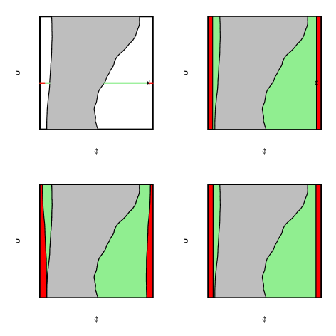
Figure 1: Comparison of the p๐‘p-value of Jewell etย al., (2022) (left-hand column) and the ideal p๐‘p-value (right-hand column) for the case of a univariate ฯˆ๐œ“\psi parameter. We have used the probability inverse mapping to transform ฯ•italic-ฯ•\phi and ฯˆ๐œ“\psi so that they are uniformly and independently distributed on [0,1]01[0,1] under the prior. We view data sets as being a function of (ฯ•,ฯˆ)italic-ฯ•๐œ“(\phi,\psi), and the selection event โ€“ which corresponds to the information in the data used to choose the test โ€“ corresponds to a region of (ฯ•,ฯˆ)italic-ฯ•๐œ“(\phi,\psi) values (non-grey region in all plots). The observed data corresponds to a specific (ฯ•,ฯˆ)italic-ฯ•๐œ“(\phi,\psi) value shown by a cross (top-row plots). For the method of Jewell etย al., (2022), the p๐‘p-value is the probability of observing a more extreme value of ฯ•italic-ฯ•\phi conditional on the observed ฯˆ๐œ“\psi-value. This is the proportion of the coloured line that is red in the top-right plot. For our method, the p๐‘p-value is the (unconditional) probability of observing a more extreme value of ฯ•italic-ฯ•\phi: the proportion of the non-grey area that is red (top-right plot). In the bottom row we show the data-sets, as represented by their (ฯ•,ฯˆ)italic-ฯ•๐œ“(\phi,\psi) value, that would give a post-selection p๐‘p-value that is 0.2 or lower (red region in both plots).

To understand the difference between the ideal post-selection p๐‘p-value (4) and the p๐‘p-value of Jewell etย al., (2022), we give a schematic comparison in Figure 1. To enable us to present a plot we have supposed that ฯˆ๐œ“\psi is scalar โ€“ we can see this as a special case where we fix all but one component of ๐๐\boldsymbol{\psi} โ€“ and have also used the probability inverse mapping to transform (ฯ•,ฯˆ)italic-ฯ•๐œ“(\phi,\psi) from independent Gaussian to independent uniform on [0,1]01[0,1].

With this mapping, and given the conditioning in (3), data sets correspond to points in (ฯ•,ฯˆ)italic-ฯ•๐œ“(\phi,\psi)-space, and under the null such points are uniform on the unit square. The conditioning on ฯ„^^๐œ\hat{\tau} being a detected changepoint corresponds to restricting the possible set of (ฯ•,ฯˆ)italic-ฯ•๐œ“(\phi,\psi) values โ€“ to the non-grey area in Figure 1. We have plotted the (ฯ•,ฯˆ)italic-ฯ•๐œ“(\phi,\psi) value for the observed data by a cross in the top row of Figure 1. The p๐‘p-value of Jewell etย al., (2022) then fixes the ฯˆ๐œ“\psi value so the conditional distribution of ฯ•italic-ฯ•\phi is uniform on the coloured line โ€“ i.e. all values that are consistent with detecting a change at ฯ„^^๐œ\hat{\tau} for that value of ฯˆ๐œ“\psi. The p๐‘p-value is the probability of observing a more extreme value than that for the data โ€“ which is the proportion of the line that is red.

By comparison, the p๐‘p-value of (4) allows ฯˆ๐œ“\psi to vary. It is thus the probability of observing a more extreme value of ฯ•italic-ฯ•\phi than that for the data over all possible (ฯ•,ฯˆ)italic-ฯ•๐œ“(\phi,\psi) values that are consistent with ฯ„^^๐œ\hat{\tau} being a detected change. This is the proportion of the non-grey area that is red in the top right plot of Figure 1. If we generate the data by simulating a (ฯ•,ฯˆ)italic-ฯ•๐œ“(\phi,\psi) point uniformly in the non-grey region, then it is simple to show that the distribution of either p๐‘p-value will be uniform on [0,1]01[0,1].

To see why the ideal p๐‘p-value (4) is to be preferred, in the bottom row of Figure 1 we plot the set of (ฯ•,ฯˆ)italic-ฯ•๐œ“(\phi,\psi) values that would correspond to data with a post-selection p๐‘p-value of less than 0.2. For both p๐‘p-values these give regions whose area is 0.2 of the non-grey area. The difference is the shape of the regions, with the ideal p๐‘p-value consisting of requiring just ฯ•italic-ฯ•\phi greater than some constant, whereas the p๐‘p-value of Jewell etย al., (2022) has different regions for ฯ•italic-ฯ•\phi as we vary ฯˆ๐œ“\psi. The former will have more power if we have alternative hypotheses that, compared to the null, place increasing probability on larger values of |ฯ•|italic-ฯ•|\phi|.

To make this precise, let ๐’œ๐’œ\mathcal{A} be the projection of the data we condition on (3). Under the null, and conditional on ๐’œ๐’œ\mathcal{A} denote the density for (ฯ•,๐)italic-ฯ•๐(\phi,\boldsymbol{\psi}) as

fโ€‹(ฯ•)โ€‹โˆi=12โ€‹hโˆ’2gโ€‹(ฯˆi).๐‘“italic-ฯ•superscriptsubscriptproduct๐‘–12โ„Ž2๐‘”subscript๐œ“๐‘–f(\phi)\prod_{i=1}^{2h-2}g(\psi_{i}).

Consider alternative hypotheses that correspond to a density of (ฯ•,๐)italic-ฯ•๐(\phi,\boldsymbol{\psi}) of the form

kโ€‹(ฯ•)โ€‹fโ€‹(ฯ•)โ€‹โˆi=12โ€‹hโˆ’2gโ€‹(ฯˆi),๐‘˜italic-ฯ•๐‘“italic-ฯ•superscriptsubscriptproduct๐‘–12โ„Ž2๐‘”subscript๐œ“๐‘–k(\phi)f(\phi)\prod_{i=1}^{2h-2}g(\psi_{i}), (5)

for some function kโ€‹(ฯ•)๐‘˜italic-ฯ•k(\phi). That is, under the alternative hypothesis the distribution of ฯ•italic-ฯ•\phi is altered, and kโ€‹(ฯ•)๐‘˜italic-ฯ•k(\phi) represents the ratio of density between the alternative and the null.

Theorem 1.

Conditional on ๐’œ๐’œ\mathcal{A} and (ฯ•,๐›™)โˆˆ๐’ฎitalic-ฯ•๐›™๐’ฎ(\phi,\boldsymbol{\psi})\in\mathcal{S}, define PIsubscript๐‘ƒ๐ผP_{I} to be the p๐‘p-value given by (4), and Pโˆ—superscript๐‘ƒP^{*} be any other valid p๐‘p-value, i.e. that satisfies that under the null

Prโก(Pโˆ—โ‰คฮฑ)โ‰คฮฑ,for allย ฮฑโˆˆ[0,1].Prsuperscript๐‘ƒ๐›ผ๐›ผfor allย ฮฑโˆˆ[0,1].\Pr(P^{*}\leq\alpha)\leq\alpha,~{}\mbox{for all $\alpha\in[0,1]$.}

Then under an alternative with density of the form (5) for a function kโ€‹(ฯ•)=k~โ€‹(|ฯ•|)๐‘˜italic-ฯ•~๐‘˜italic-ฯ•k(\phi)=\tilde{k}(|\phi|) with k~~๐‘˜\tilde{k} increasing,

Prโก(PIโ‰คฮฑ)โ‰ฅPrโก(Pโˆ—โ‰คฮฑ),for allย ฮฑโˆˆ[0,1].Prsubscript๐‘ƒ๐ผ๐›ผPrsuperscript๐‘ƒ๐›ผfor allย ฮฑโˆˆ[0,1].\Pr(P_{I}\leq\alpha)\geq\Pr(P^{*}\leq\alpha),~{}\mbox{for all $\alpha\in[0,1]$.}

The condition that the distribution under the alternative is of form (5) for appropriate kโ€‹(ฯ•)๐‘˜italic-ฯ•k(\phi), holds if under the alternative we have a common mean for Xฯ„^โˆ’h+1,โ€ฆ,Xฯ„^subscript๐‘‹^๐œโ„Ž1โ€ฆsubscript๐‘‹^๐œX_{\hat{\tau}-h+1},\ldots,X_{\hat{\tau}}, and a different common mean for Xฯ„^+1,โ€ฆ,Xฯ„^+hsubscript๐‘‹^๐œ1โ€ฆsubscript๐‘‹^๐œโ„ŽX_{\hat{\tau}+1},\ldots,X_{\hat{\tau}+h}, and that the density for the size of the change in mean is symmetric about 0 โ€“ see Appendix A.1 for details.

3.3 Estimating p๐‘p-values with sampling

Unfortunately it is not possible to analytically calculate the ideal post-selection p๐‘p-value (4). Instead we will resort to using Monte Carlo to estimate it, under the assumption that we have a method for calculating the null distribution of ฯ•italic-ฯ•\phi given ๐๐\boldsymbol{\psi} โ€“ this would refer to any combination of type of change, choice of null hypothesis and method for detecting the changepoints for which current post-selection inference methods exist.

Let

๐’ฎ={(ฯ•,๐):ฯ„^โˆˆโ„ณโ€‹(๐‘ฟโ€ฒโ€‹(ฯ•,๐))},๐’ฎconditional-setitalic-ฯ•๐^๐œโ„ณsuperscript๐‘ฟโ€ฒitalic-ฯ•๐\mathcal{S}=\{(\phi,\boldsymbol{\psi}):\hat{\tau}\in\mathcal{M}\left(\boldsymbol{X}^{\prime}(\phi,\boldsymbol{\psi})\right)\},

so the conditioning event for (4) corresponds to (ฯ•,๐)italic-ฯ•๐(\phi,\boldsymbol{\psi}). Furthermore, define

๐’ฎ๐={ฯ•:ฯ„^โˆˆโ„ณโ€‹(๐‘ฟโ€ฒโ€‹(ฯ•,๐))},subscript๐’ฎ๐conditional-setitalic-ฯ•^๐œโ„ณsuperscript๐‘ฟโ€ฒitalic-ฯ•๐\mathcal{S}_{\boldsymbol{\psi}}=\{\phi:\hat{\tau}\in\mathcal{M}\left(\boldsymbol{X}^{\prime}(\phi,\boldsymbol{\psi})\right)\},

the set of ฯ•italic-ฯ•\phi values corresponding to data where we estimate ฯ„^^๐œ\hat{\tau} as a changepoint, for a given value of ๐๐\boldsymbol{\psi}. These regions ๐’ฎ๐subscript๐’ฎ๐\mathcal{S}_{\boldsymbol{\psi}} will depend on the algorithm used to estimate the changepoints, but we can make use of existing methods to calculate them. For example, Jewell etย al., (2022) show how to calculate these regions for the change in mean problem with changepoints estimated by binary segmentation (their method is easily extended to variants such as wild binary segmentation and narrowest over threshold) and L0subscript๐ฟ0L_{0} penalised likelihood methods. In each case the set ๐’ฎ๐subscript๐’ฎ๐\mathcal{S}_{\boldsymbol{\psi}} consists of a finite union of intervals in ฯ•italic-ฯ•\phi.

Now that we have 2โ€‹hโˆ’22โ„Ž22h-2 additional parameters in ๐๐\boldsymbol{\psi}, the truncation region ๐’ฎ๐’ฎ\mathcal{S} becomes much more complicated to calculate explicitly, as the values of ฯ•italic-ฯ•\phi that yield ฯ„^โˆˆโ„ณโ€‹(๐‘ฟโ€ฒโ€‹(ฯ•))^๐œโ„ณsuperscript๐‘ฟโ€ฒitalic-ฯ•\hat{\tau}\in\mathcal{M}(\boldsymbol{X}^{\prime}(\phi)) depend on ๐๐\boldsymbol{\psi}. However, for a given ๐โˆ—superscript๐\boldsymbol{\psi}^{*}, by replacing ๐‘ฟ๐‘ฟ\boldsymbol{X} with ๐‘ฟฯˆโˆ—=๐‘ผโ€‹๐šฟโˆ—+1โ€–๐‚ฯ„^โ€–22โ€‹๐‚ฯ„^โ€‹๐‚ฯ„^Tโ€‹๐‘ฟ+1โ€–๐’‚โ€–22โ€‹๐’‚โ€‹๐’‚Tโ€‹๐‘ฟ+๐‘ฉโ€‹๐‘ฉTโ€‹๐‘ฟsubscript๐‘ฟsuperscript๐œ“๐‘ผsuperscript๐šฟ1superscriptsubscriptnormsubscript๐‚^๐œ22subscript๐‚^๐œsuperscriptsubscript๐‚^๐œ๐‘‡๐‘ฟ1superscriptsubscriptnorm๐’‚22๐’‚superscript๐’‚๐‘‡๐‘ฟ๐‘ฉsuperscript๐‘ฉ๐‘‡๐‘ฟ\boldsymbol{X}_{\psi^{*}}=\boldsymbol{U\Psi}^{*}+\frac{1}{||\boldsymbol{\nu}_{\hat{\tau}}||_{2}^{2}}\boldsymbol{\nu}_{\hat{\tau}}\boldsymbol{\nu}_{\hat{\tau}}^{T}\boldsymbol{X}+\frac{1}{||\boldsymbol{a}||_{2}^{2}}\boldsymbol{aa}^{T}\boldsymbol{X}+\boldsymbol{BB}^{T}\boldsymbol{X}, we can calculate ๐’ฎฯˆโˆ—subscript๐’ฎsuperscript๐œ“\mathcal{S}_{\psi^{*}} using the method of Jewell etย al., (2022). We can then calculate a p๐‘p-value conditional on ๐โˆ—superscript๐\boldsymbol{\psi}^{*}:

pฯˆโˆ—=Prโก(|ฯ•|โ‰ฅ|๐‚ฯ„^Tโ€‹๐‘ฟoโ€‹bโ€‹s|โˆฉฯ•โˆˆ๐’ฎฯˆโˆ—)Prโก(ฯ•โˆˆ๐’ฎฯˆโˆ—).subscript๐‘superscript๐œ“Pritalic-ฯ•superscriptsubscript๐‚^๐œ๐‘‡subscript๐‘ฟ๐‘œ๐‘๐‘ italic-ฯ•subscript๐’ฎsuperscript๐œ“Pritalic-ฯ•subscript๐’ฎsuperscript๐œ“p_{\psi^{*}}=\frac{\Pr(|\phi|\geq|\boldsymbol{\nu}_{\hat{\tau}}^{T}\boldsymbol{X}_{obs}|\cap\phi\in\mathcal{S}_{\psi^{*}})}{\Pr(\phi\in\mathcal{S}_{\psi^{*}})}.

To estimate the overall p๐‘p-value, we take N๐‘N samples, {๐(1),โ€ฆ,๐(N)}superscript๐1โ€ฆsuperscript๐๐‘\{\boldsymbol{\psi}^{(1)},\ldots,\boldsymbol{\psi}^{(N)}\}, and calculate ๐’ฎ๐(j)subscript๐’ฎsuperscript๐๐‘—\mathcal{S}_{\boldsymbol{\psi}^{(j)}} for each ๐(j)superscript๐๐‘—\boldsymbol{\psi}^{(j)}. We then estimate the p๐‘p-value as

Prโก(|ฯ•|โ‰ฅ|๐‚ฯ„^Tโ€‹๐‘ฟoโ€‹bโ€‹s|โˆฉฯ•โˆˆ๐’ฎ)Prโก(ฯ•โˆˆ๐’ฎ)โ‰ˆ1Nโ€‹โˆ‘j=1NPrโก(|ฯ•|โ‰ฅ|๐‚ฯ„^Tโ€‹๐‘ฟoโ€‹bโ€‹s|โˆฉฯ•โˆˆ๐’ฎ๐(j))1Nโ€‹โˆ‘j=1NPrโก(ฯ•โˆˆ๐’ฎ๐(j))=p^N.Pritalic-ฯ•superscriptsubscript๐‚^๐œ๐‘‡subscript๐‘ฟ๐‘œ๐‘๐‘ italic-ฯ•๐’ฎPritalic-ฯ•๐’ฎ1๐‘superscriptsubscript๐‘—1๐‘Pritalic-ฯ•superscriptsubscript๐‚^๐œ๐‘‡subscript๐‘ฟ๐‘œ๐‘๐‘ italic-ฯ•subscript๐’ฎsuperscript๐๐‘—1๐‘superscriptsubscript๐‘—1๐‘Pritalic-ฯ•subscript๐’ฎsuperscript๐๐‘—subscript^๐‘๐‘\frac{\Pr(|\phi|\geq|\boldsymbol{\nu}_{\hat{\tau}}^{T}\boldsymbol{X}_{obs}|\cap\phi\in\mathcal{S})}{\Pr(\phi\in\mathcal{S})}\approx\frac{\frac{1}{N}\sum_{j=1}^{N}\Pr(|\phi|\geq|\boldsymbol{\nu}_{\hat{\tau}}^{T}\boldsymbol{X}_{obs}|\cap\phi\in\mathcal{S}_{\boldsymbol{\psi}^{(j)}})}{\frac{1}{N}\sum_{j=1}^{N}\Pr(\phi\in\mathcal{S}_{\boldsymbol{\psi}^{(j)}})}=\hat{p}_{N}. (6)

This can also be written as a weighted average of individual p๐‘p-value estimates

p^N=1โˆ‘j=1Nwjโ€‹โˆ‘j=1Nwjโ€‹pฯˆ(j),subscript^๐‘๐‘1superscriptsubscript๐‘—1๐‘subscript๐‘ค๐‘—superscriptsubscript๐‘—1๐‘subscript๐‘ค๐‘—subscript๐‘superscript๐œ“๐‘—\hat{p}_{N}=\frac{1}{\sum_{j=1}^{N}w_{j}}\sum_{j=1}^{N}w_{j}p_{\psi^{(j)}}, (7)

where wj=Prโก(ฯ•โˆˆ๐’ฎ๐(j))subscript๐‘ค๐‘—Pritalic-ฯ•subscript๐’ฎsuperscript๐๐‘—w_{j}=\Pr(\phi\in\mathcal{S}_{\boldsymbol{\psi}^{(j)}}). Since each ๐’ฎ๐(j)subscript๐’ฎsuperscript๐๐‘—\mathcal{S}_{\boldsymbol{\psi}^{(j)}} consists of a union of intervals, and ฯ•โˆผNโ€‹(0,2โ€‹ฯƒ2h)similar-toitalic-ฯ•๐‘02superscript๐œŽ2โ„Ž\phi\sim N(0,\frac{2\sigma^{2}}{h}), it is straightforward to calculate wjsubscript๐‘ค๐‘—w_{j} and p๐(j)subscript๐‘superscript๐๐‘—p_{\boldsymbol{\psi}^{(j)}}.

Refer to caption

(a)h=10โ„Ž10h=10Refer to caption(b)h=20โ„Ž20h=20Refer to caption(c)h=10โ„Ž10h=10Refer to caption(d)h=20โ„Ž20h=20

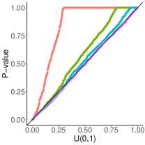
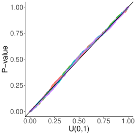
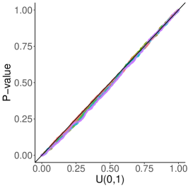
Figure 2: QQ plots of p๐‘p-value estimates, simulated under H0subscript๐ป0H_{0} with T=1000๐‘‡1000T=1000, for different values of hโ„Žh and N๐‘N. On each plot the ordered p๐‘p-values obtained using different values of N๐‘N (N=1,5,10,50๐‘151050N=1,5,10,50) are plotted against theoretical quantiles from Uโ€‹(0,1)๐‘ˆ01U(0,1). In (a) and (b) the p๐‘p-values are calculated as in Equation 6, where all ๐(j)superscript๐๐‘—\boldsymbol{\psi}^{(j)}โ€™s are simulated randomly. In (c) and (d), we take ๐(1)=๐‘ผTโ€‹๐‘ฟoโ€‹bโ€‹ssuperscript๐1superscript๐‘ผ๐‘‡subscript๐‘ฟ๐‘œ๐‘๐‘ \boldsymbol{\psi}^{(1)}=\boldsymbol{U}^{T}\boldsymbol{X}_{obs}. If p๐‘p-values are valid, the points should lie approximately along the line y=x๐‘ฆ๐‘ฅy=x.

As Nโ†’โˆžโ†’๐‘N\rightarrow\infty this Monte Carlo estimate will converge to the ideal post-selection p๐‘p-value (4). However for finite N๐‘N it will not necessarily be a valid p๐‘p-value, in that there is no guarantee that under the null, and conditional on choosing to test the null, that the p๐‘p-value will be uniformly distributed on [0,1]01[0,1].

To see this, we simulated this Monte Carlo p๐‘p-value for different values of N๐‘N: see Figure 2(a) and (b). We see that, in particular, there is a non-trivial probability that some p^ฯˆ(j)=1subscript^๐‘superscript๐œ“๐‘—1\hat{p}_{\psi^{(j)}}=1, as for some values of ๐๐\boldsymbol{\psi} we have ๐’ฎ๐โŠ‚{ฯ•:|ฯ•|โ‰ฅ|๐‚ฯ„^Tโ€‹๐‘ฟoโ€‹bโ€‹s|}subscript๐’ฎ๐conditional-setitalic-ฯ•italic-ฯ•superscriptsubscript๐‚^๐œ๐‘‡subscript๐‘ฟ๐‘œ๐‘๐‘ \mathcal{S}_{\boldsymbol{\psi}}\subset\{\phi:|\phi|\geq|\boldsymbol{\nu}_{\hat{\tau}}^{T}\boldsymbol{X}_{obs}|\}.

Remarkably, we can overcome these issues by just setting one of the ๐๐\boldsymbol{\psi} values to be the value for the observed data. Remember that ๐=๐‘ผTโ€‹๐‘ฟ๐superscript๐‘ผ๐‘‡๐‘ฟ\boldsymbol{\psi}=\boldsymbol{U}^{T}\boldsymbol{X}. Let ๐(1)=๐‘ผTโ€‹๐‘ฟoโ€‹bโ€‹ssuperscript๐1superscript๐‘ผ๐‘‡subscript๐‘ฟ๐‘œ๐‘๐‘ \boldsymbol{\psi}^{(1)}=\boldsymbol{U}^{T}\boldsymbol{X}_{obs}. Simulate ๐(2),โ€ฆ,๐(N)superscript๐2โ€ฆsuperscript๐๐‘\boldsymbol{\psi}^{(2)},\ldots,\boldsymbol{\psi}^{(N)} independently from the null distribution for ๐๐\boldsymbol{\psi}, and calculate the p๐‘p-value as p^Nsubscript^๐‘๐‘\hat{p}_{N} in (6).

The following theorem shows that the resulting post-selection p๐‘p-value will be distributed uniformly on [0,1]01[0,1] under the null, for any value of N๐‘N.

Theorem 2.

Let

p^N=1โˆ‘j=1Nwjโ€‹โˆ‘j=1Nwjโ€‹pฯˆ(j),subscript^๐‘๐‘1superscriptsubscript๐‘—1๐‘subscript๐‘ค๐‘—superscriptsubscript๐‘—1๐‘subscript๐‘ค๐‘—subscript๐‘superscript๐œ“๐‘—\hat{p}_{N}=\frac{1}{\sum_{j=1}^{N}w_{j}}\sum_{j=1}^{N}w_{j}p_{\psi^{(j)}},

where wj=Prโก(ฯ•โˆˆ๐’ฎฯˆ(j))subscript๐‘ค๐‘—Pritalic-ฯ•subscript๐’ฎsuperscript๐œ“๐‘—w_{j}=\Pr(\phi\in\mathcal{S}_{\psi^{(j)}}). Given that there is one jโˆ—โˆˆ{1,โ€ฆ,N}superscript๐‘—1โ€ฆ๐‘j^{*}\in\{1,\ldots,N\} such that ฯˆ(jโˆ—)superscript๐œ“superscript๐‘—\psi^{(j^{*})} corresponds to the observed data, and that other ฯˆ(j)superscript๐œ“๐‘—\psi^{(j)} are drawn independently from their distribution under the null, then under H0subscript๐ป0H_{0}, p^NโˆผUโ€‹(0,1)similar-tosubscript^๐‘๐‘๐‘ˆ01\hat{p}_{N}\sim U(0,1).

Figure 2 (c) and (d) show empirical validation of this result. An important consequence is that p^Nsubscript^๐‘๐‘\hat{p}_{N} is a valid p๐‘p-value for any value of N๐‘N, even if computational constraints limit N๐‘N to be small. Below, in Section 4, we show that even small to moderate values of N๐‘N can lead to a substantial increase in power.

3.4 Extension to other null hypotheses

So far, we have calculated p๐‘p-values for the change in mean model, based on the assumption that there are no other changepoints within a fixed window hโ„Žh of ฯ„^^๐œ\hat{\tau}. However, we can also apply our method to a range of other scenarios, such as different null hypotheses and different types of changepoint model. This may lead to different choices for ฯ•italic-ฯ•\phi and โ„ฑโ€‹(๐‘ฟ)โ„ฑ๐‘ฟ\mathcal{F}(\boldsymbol{X}), but as long as we can define ๐๐\boldsymbol{\psi} and have a method for calculating ๐’ฎ๐subscript๐’ฎ๐\mathcal{S}_{\boldsymbol{\psi}}, we can still use our method. We outline some examples below.

We discuss first the choice of null hypothesis. Rather than assume that the mean is constant within a fixed window of size hโ„Žh on either side of ฯ„^^๐œ\hat{\tau}, we can consider the more general case where H0subscript๐ป0H_{0} is of the form

ฮผฯ„^โˆ’h1+1=โ€ฆ=ฮผฯ„^=ฮผฯ„^+1=โ€ฆ=ฮผฯ„^+h2subscript๐œ‡^๐œsubscriptโ„Ž11โ€ฆsubscript๐œ‡^๐œsubscript๐œ‡^๐œ1โ€ฆsubscript๐œ‡^๐œsubscriptโ„Ž2\mu_{\hat{\tau}-h_{1}+1}=\ldots=\mu_{\hat{\tau}}=\mu_{\hat{\tau}+1}=\ldots=\mu_{\hat{\tau}+h_{2}}

for some integers h1,h2subscriptโ„Ž1subscriptโ„Ž2h_{1},h_{2}, where these can be either fixed in advance or selected based on the locations of neighbouring changepoints. We define ๐‚ฯ„^subscript๐‚^๐œ\boldsymbol{\nu}_{\hat{\tau}} as

(๐‚ฯ„^)t={1h1ifย โ€‹ฯ„^โˆ’h1<tโ‰คฯ„^โˆ’1h2ifย โ€‹ฯ„^<tโ‰คฯ„^+h20ifย โ€‹tโ‰คฯ„^โˆ’h1โ€‹ย orย โ€‹t>ฯ„^+h2.subscriptsubscript๐‚^๐œ๐‘กcases1subscriptโ„Ž1ifย ^๐œsubscriptโ„Ž1๐‘ก^๐œ1subscriptโ„Ž2ifย ^๐œ๐‘ก^๐œsubscriptโ„Ž20ifย ๐‘ก^๐œsubscriptโ„Ž1ย orย ๐‘ก^๐œsubscriptโ„Ž2(\boldsymbol{\nu}_{\hat{\tau}})_{t}=\begin{cases}\frac{1}{h_{1}}&\text{if }\hat{\tau}-h_{1}<t\leq\hat{\tau}\\ -\frac{1}{h_{2}}&\text{if }\hat{\tau}<t\leq\hat{\tau}+h_{2}\\ 0&\text{if }t\leq\hat{\tau}-h_{1}\text{ or }t>\hat{\tau}+h_{2}.\end{cases}

The null hypothesis we have previously considered is the special case that h1=h2=hsubscriptโ„Ž1subscriptโ„Ž2โ„Žh_{1}=h_{2}=h.

A modification which avoids the problem having of other detected changepoints within the region of interest is to choose a pre-determined hโ„Žh but truncate the region if another changepoint is detected within hโ„Žh of ฯ„^^๐œ\hat{\tau}. Denoting the changepoint of interest as ฯ„^jsubscript^๐œ๐‘—\hat{\tau}_{j} (where jโˆˆ{1,โ€ฆ,K}๐‘—1โ€ฆ๐พj\in\{1,\ldots,K\}), we hence take h1=minโก{h,ฯ„^jโˆ’ฯ„^jโˆ’1}subscriptโ„Ž1โ„Žsubscript^๐œ๐‘—subscript^๐œ๐‘—1h_{1}=\min\{h,\hat{\tau}_{j}-\hat{\tau}_{j-1}\} and h2=minโก{h,ฯ„^j+1โˆ’ฯ„^j}subscriptโ„Ž2โ„Žsubscript^๐œ๐‘—1subscript^๐œ๐‘—h_{2}=\min\{h,\hat{\tau}_{j+1}-\hat{\tau}_{j}\}. Alternatively, we can allow the region of interest to be determined by the changepoints on either side of ฯ„^jsubscript^๐œ๐‘—\hat{\tau}_{j}: either by taking it to be all points between the two neighbouring changepoints (ฯ„^jโˆ’1,ฯ„^j+1)subscript^๐œ๐‘—1subscript^๐œ๐‘—1(\hat{\tau}_{j-1},\hat{\tau}_{j+1}), thus h1=ฯ„^jโˆ’ฯ„^jโˆ’1subscriptโ„Ž1subscript^๐œ๐‘—subscript^๐œ๐‘—1h_{1}=\hat{\tau}_{j}-\hat{\tau}_{j-1} and h2=ฯ„^j+1โˆ’ฯ„^jsubscriptโ„Ž2subscript^๐œ๐‘—1subscript^๐œ๐‘—h_{2}=\hat{\tau}_{j+1}-\hat{\tau}_{j} โ€“ this is the scenario used in Hyun etย al., (2021), and is also considered in Jewell etย al., (2022) โ€“ or by taking it to be the set of points which are closer to ฯ„^jsubscript^๐œ๐‘—\hat{\tau}_{j} than to neighbouring changepoints, so h1=โŒŠฯ„^jโˆ’ฯ„^jโˆ’12โŒ‹subscriptโ„Ž1subscript^๐œ๐‘—subscript^๐œ๐‘—12h_{1}=\lfloor\frac{\hat{\tau}_{j}-\hat{\tau}_{j-1}}{2}\rfloor and h2=โŒŠฯ„^j+1โˆ’ฯ„^j2โŒ‹subscriptโ„Ž2subscript^๐œ๐‘—1subscript^๐œ๐‘—2h_{2}=\lfloor\frac{\hat{\tau}_{j}+1-\hat{\tau}_{j}}{2}\rfloor. In general, the choice of null hypothesis will depend on what is appropriate for the application.

In any of these cases, we can apply our method in the same way as for the special case so far considered. The one possible difference is the choice of โ„ฑโ„ฑ\mathcal{F}: if H0subscript๐ป0H_{0} depends on the locations of other estimated changepoints besides ฯ„^^๐œ\hat{\tau}, then we must condition on the locations of all estimated changepoints rather than just whether ฯ„^^๐œ\hat{\tau} is included in the model. So, in this case we replace the condition ฯ„^โˆˆโ„ณโ€‹(๐‘ฟ)^๐œโ„ณ๐‘ฟ\hat{\tau}\in\mathcal{M}(\boldsymbol{X}) in Equation 4 with โ„ณโ€‹(๐‘ฟโ€ฒโ€‹(ฯ•,๐))=โ„ณโ€‹(๐‘ฟoโ€‹bโ€‹s)โ„ณsuperscript๐‘ฟโ€ฒitalic-ฯ•๐โ„ณsubscript๐‘ฟ๐‘œ๐‘๐‘ \mathcal{M}(\boldsymbol{X}^{\prime}(\phi,\boldsymbol{\psi}))=\mathcal{M}(\boldsymbol{X}_{obs}), to get the p๐‘p-value

p=Prฯ•โก(|ฯ•|โ‰ฅ|๐‚ฯ„^Tโ€‹๐‘ฟoโ€‹bโ€‹s||โ„ณโ€‹(๐‘ฟโ€ฒโ€‹(ฯ•,๐))=โ„ณโ€‹(๐‘ฟoโ€‹bโ€‹s)).๐‘subscriptPritalic-ฯ•italic-ฯ•conditionalsuperscriptsubscript๐‚^๐œ๐‘‡subscript๐‘ฟ๐‘œ๐‘๐‘ โ„ณsuperscript๐‘ฟโ€ฒitalic-ฯ•๐โ„ณsubscript๐‘ฟ๐‘œ๐‘๐‘ p=\Pr_{\phi}\left(|\phi|\geq|\boldsymbol{\nu}_{\hat{\tau}}^{T}\boldsymbol{X}_{obs}|~{}~{}|~{}~{}\mathcal{M}(\boldsymbol{X}^{\prime}(\phi,\boldsymbol{\psi}))=\mathcal{M}(\boldsymbol{X}_{obs})\right).

This can be seen as a special case, since, given ฯ„^โˆˆโ„ณโ€‹(๐‘ฟoโ€‹bโ€‹s)^๐œโ„ณsubscript๐‘ฟ๐‘œ๐‘๐‘ \hat{\tau}\in\mathcal{M}(\boldsymbol{X}_{obs}), {ฯ•|โ„ณโ€‹(๐‘ฟโ€ฒโ€‹(ฯ•,๐))=โ„ณโ€‹(๐‘ฟoโ€‹bโ€‹s)}โŠ†{ฯ•|ฯ„^โˆˆโ„ณโ€‹(๐‘ฟโ€ฒโ€‹(ฯ•,๐))}conditional-setitalic-ฯ•โ„ณsuperscript๐‘ฟโ€ฒitalic-ฯ•๐โ„ณsubscript๐‘ฟ๐‘œ๐‘๐‘ conditional-setitalic-ฯ•^๐œโ„ณsuperscript๐‘ฟโ€ฒitalic-ฯ•๐\{\phi~{}|~{}\mathcal{M}(\boldsymbol{X}^{\prime}(\phi,\boldsymbol{\psi}))=\mathcal{M}(\boldsymbol{X}_{obs})\}\subseteq\{\phi~{}|~{}\hat{\tau}\in\mathcal{M}(\boldsymbol{X}^{\prime}(\phi,\boldsymbol{\psi}))\}. Jewell etย al., (2022) provides a method to compute this set for fixed ๐๐\boldsymbol{\psi}, so we can apply the same method as in Section 3.3.

It is also possible to apply our methods to different sorts of models. For example, we consider the model of Chen etย al., (2023). They use a model of the form

Xt=ct+ฯตt,t=1,โ€ฆ,T,formulae-sequencesubscript๐‘‹๐‘กsubscript๐‘๐‘กsubscriptitalic-ฯต๐‘ก๐‘ก1โ€ฆ๐‘‡X_{t}=c_{t}+\epsilon_{t},~{}~{}t=1,\ldots,T,

where ฯตtโˆผNโ€‹(0,ฯƒ2)similar-tosubscriptitalic-ฯต๐‘ก๐‘0superscript๐œŽ2\epsilon_{t}\sim N(0,\sigma^{2}) and ct=ฮณโ€‹ctโˆ’1+ztsubscript๐‘๐‘ก๐›พsubscript๐‘๐‘ก1subscript๐‘ง๐‘กc_{t}=\gamma c_{t-1}+z_{t}, with zt=0subscript๐‘ง๐‘ก0z_{t}=0 except at changepoints and ฮณ๐›พ\gamma assumed known.

In the paper they develop a selective inference procedure similar to the methods in Jewell etย al., (2022), where they fix a window of size hโ„Žh around an estimated change ฯ„^^๐œ\hat{\tau}, and take as the null hypothesis that there are no changes within this window: i.e.

(cฯ„^โˆ’h+1,cฯ„^โˆ’h+2,โ€ฆ,cฯ„^,โ€ฆ,cฯ„^+h)=(ฮณโˆ’h+1,ฮณโˆ’h+2,โ€ฆ,ฮณ0,โ€ฆ,ฮณh)โ€‹cฯ„^.subscript๐‘^๐œโ„Ž1subscript๐‘^๐œโ„Ž2โ€ฆsubscript๐‘^๐œโ€ฆsubscript๐‘^๐œโ„Žsuperscript๐›พโ„Ž1superscript๐›พโ„Ž2โ€ฆsuperscript๐›พ0โ€ฆsuperscript๐›พโ„Žsubscript๐‘^๐œ\left(c_{\hat{\tau}-h+1},c_{\hat{\tau}-h+2},\ldots,c_{\hat{\tau}},\ldots,c_{\hat{\tau}+h}\right)=\left(\gamma^{-h+1},\gamma^{-h+2},\ldots,\gamma^{0},\ldots,\gamma^{h}\right)c_{\hat{\tau}}.

This leads to a test statistic ๐‚Tโ€‹๐‘ฟsuperscript๐‚๐‘‡๐‘ฟ\boldsymbol{\nu}^{T}\boldsymbol{X}, where ๐‚๐‚\boldsymbol{\nu} is defined as

๐‚={โˆ’ฮณโ€‹(ฮณ2โˆ’1)ฮณ2โˆ’ฮณโˆ’2โ€‹h+2โ€‹ฮณtโˆ’ฯ„^ifย โ€‹ฯ„^โˆ’h<tโ‰คฯ„^ฮณ2โˆ’1ฮณ2โ€‹hโˆ’1โ€‹ฮณtโˆ’ฯ„^โˆ’1ifย โ€‹ฯ„^<tโ‰คฯ„^+h0ifย โ€‹tโ‰คฯ„^โˆ’hโ€‹ย orย โ€‹t>ฯ„^+h.๐‚cases๐›พsuperscript๐›พ21superscript๐›พ2superscript๐›พ2โ„Ž2superscript๐›พ๐‘ก^๐œifย ^๐œโ„Ž๐‘ก^๐œsuperscript๐›พ21superscript๐›พ2โ„Ž1superscript๐›พ๐‘ก^๐œ1ifย ^๐œ๐‘ก^๐œโ„Ž0ifย ๐‘ก^๐œโ„Žย orย ๐‘ก^๐œโ„Ž\boldsymbol{\nu}=\begin{cases}-\frac{\gamma(\gamma^{2}-1)}{\gamma^{2}-\gamma^{-2h+2}}\gamma^{t-\hat{\tau}}&\text{if }\hat{\tau}-h<t\leq\hat{\tau}\\ \frac{\gamma^{2}-1}{\gamma^{2h}-1}\gamma^{t-\hat{\tau}-1}&\text{if }\hat{\tau}<t\leq\hat{\tau}+h\\ 0&\text{if }t\leq\hat{\tau}-h\text{ or }t>\hat{\tau}+h.\end{cases}

Letting ฯ•=๐‚Tโ€‹๐‘ฟitalic-ฯ•superscript๐‚๐‘‡๐‘ฟ\phi=\boldsymbol{\nu}^{T}\boldsymbol{X} as before and conditioning on ๐šทฯ„^โ€‹๐‘ฟ=๐šทฯ„^โ€‹๐‘ฟoโ€‹bโ€‹ssubscript๐šท^๐œ๐‘ฟsubscript๐šท^๐œsubscript๐‘ฟ๐‘œ๐‘๐‘ \boldsymbol{\Pi}_{\hat{\tau}}\boldsymbol{X}=\boldsymbol{\Pi}_{\hat{\tau}}\boldsymbol{X}_{obs}, they show how to calculate the set ๐’ฎ={ฯ•:ฯ„^โˆˆโ„ณโ€‹(๐‘ฟโ€ฒโ€‹(ฯ•))}๐’ฎconditional-setitalic-ฯ•^๐œโ„ณsuperscript๐‘ฟโ€ฒitalic-ฯ•\mathcal{S}=\{\phi:\hat{\tau}\in\mathcal{M}(\boldsymbol{X}^{\prime}(\phi))\}, and so to calculate the p๐‘p-value

Prโก(ฯ•โ‰ฅ๐‚Tโ€‹๐‘ฟoโ€‹bโ€‹s|ฯ•โˆˆ๐’ฎ),Pritalic-ฯ•conditionalsuperscript๐‚๐‘‡subscript๐‘ฟ๐‘œ๐‘๐‘ italic-ฯ•๐’ฎ\Pr\left(\phi\geq\boldsymbol{\nu}^{T}\boldsymbol{X}_{obs}|\phi\in\mathcal{S}\right),

where ๐‘ฟโ€ฒโ€‹(ฯ•)superscript๐‘ฟโ€ฒitalic-ฯ•\boldsymbol{X}^{\prime}(\phi) is defined as in Equation 2.

As before, in our approach we condition on the values of ๐‘ฟ๐‘ฟ\boldsymbol{X} outside of the window (ฯ„^โˆ’h+1,ฯ„^+h)^๐œโ„Ž1^๐œโ„Ž(\hat{\tau}-h+1,\hat{\tau}+h); this is equivalent to fixing the value of ๐‘ฉTโ€‹๐‘ฟsuperscript๐‘ฉ๐‘‡๐‘ฟ\boldsymbol{B}^{T}\boldsymbol{X} where ๐‘ฉ๐‘ฉ\boldsymbol{B} is the Tร—(Tโˆ’2โ€‹h)๐‘‡๐‘‡2โ„ŽT\times\left(T-2h\right) matrix obtained by removing the columns corresponding to {ฯ„^โˆ’h+1,โ€ฆ,ฯ„^+h}^๐œโ„Ž1โ€ฆ^๐œโ„Ž\{\hat{\tau}-h+1,\ldots,\hat{\tau}+h\} from the Tร—T๐‘‡๐‘‡T\times T identity matrix. We also need to account for the unknown parameter cฯ„^subscript๐‘^๐œc_{\hat{\tau}} within this window. Letting ๐’‚๐’‚\boldsymbol{a} be defined as

at={ฮณtโˆ’ฯ„^ifย โ€‹ฯ„^โˆ’h+1โ‰คtโ‰คฯ„^+h0otherwise,subscript๐‘Ž๐‘กcasessuperscript๐›พ๐‘ก^๐œifย ^๐œโ„Ž1๐‘ก^๐œโ„Ž0otherwisea_{t}=\begin{cases}\gamma^{t-\hat{\tau}}&\text{if }\hat{\tau}-h+1\leq t\leq\hat{\tau}+h\\ 0&\text{otherwise},\end{cases}

we condition on c^ฯ„^=1โ€–๐’‚โ€–2โ€‹๐’‚Tโ€‹๐‘ฟsubscript^๐‘^๐œ1subscriptnorm๐’‚2superscript๐’‚๐‘‡๐‘ฟ\hat{c}_{\hat{\tau}}=\frac{1}{||\boldsymbol{a}||_{2}}\boldsymbol{a}^{T}\boldsymbol{X}, which is a sufficient statistic for cฯ„^subscript๐‘^๐œc_{\hat{\tau}}. (It can be shown that ๐’‚๐’‚\boldsymbol{a} and ๐‚๐‚\boldsymbol{\nu} as defined here are orthogonal.)

Having defined ๐‚,๐’‚๐‚๐’‚\boldsymbol{\nu},\boldsymbol{a} and ๐‘ฉ๐‘ฉ\boldsymbol{B}, we can then write, as in Section 3.1,

๐‘ฟ=๐’โ€‹๐‘ฟ+1โ€–๐‚โ€–22โ€‹๐‚โ€‹๐‚Tโ€‹๐‘ฟ+(1โ€–๐’‚โ€–22โ€‹๐’‚โ€‹๐’‚T+๐‘ฉโ€‹๐‘ฉT)โ€‹๐‘ฟoโ€‹bโ€‹s,๐‘ฟ๐’๐‘ฟ1superscriptsubscriptnorm๐‚22๐‚superscript๐‚๐‘‡๐‘ฟ1superscriptsubscriptnorm๐’‚22๐’‚superscript๐’‚๐‘‡๐‘ฉsuperscript๐‘ฉ๐‘‡subscript๐‘ฟ๐‘œ๐‘๐‘ \boldsymbol{X}=\boldsymbol{ZX}+\frac{1}{||\boldsymbol{\nu}||_{2}^{2}}\boldsymbol{\nu\nu}^{T}\boldsymbol{X}+\left(\frac{1}{||\boldsymbol{a}||_{2}^{2}}\boldsymbol{aa}^{T}+\boldsymbol{BB}^{T}\right)\boldsymbol{X}_{obs},

where ๐’=๐‘ฐโˆ’(๐‘ฉโ€‹๐‘ฉT+1โ€–๐’‚โ€–22โ€‹๐’‚โ€‹๐’‚T+1โ€–๐‚ฯ„^โ€–22โ€‹๐‚ฯ„^โ€‹๐‚ฯ„^T)๐’๐‘ฐ๐‘ฉsuperscript๐‘ฉ๐‘‡1superscriptsubscriptnorm๐’‚22๐’‚superscript๐’‚๐‘‡1superscriptsubscriptnormsubscript๐‚^๐œ22subscript๐‚^๐œsuperscriptsubscript๐‚^๐œ๐‘‡\boldsymbol{Z}=\boldsymbol{I}-\left(\boldsymbol{BB}^{T}+\frac{1}{||\boldsymbol{a}||_{2}^{2}}\boldsymbol{aa}^{T}+\frac{1}{||\boldsymbol{\nu}_{\hat{\tau}}||_{2}^{2}}\boldsymbol{\nu}_{\hat{\tau}}\boldsymbol{\nu}_{\hat{\tau}}^{T}\right), and hence

๐‘ฟโ€ฒโ€‹(ฯ•,๐)=๐‘ผโ€‹๐+1โ€–๐‚โ€–22โ€‹๐‚โ€‹ฯ•+(1โ€–๐’‚โ€–22โ€‹๐’‚โ€‹๐’‚T+๐‘ฉโ€‹๐‘ฉT)โ€‹๐‘ฟoโ€‹bโ€‹s,superscript๐‘ฟโ€ฒitalic-ฯ•๐๐‘ผ๐1superscriptsubscriptnorm๐‚22๐‚italic-ฯ•1superscriptsubscriptnorm๐’‚22๐’‚superscript๐’‚๐‘‡๐‘ฉsuperscript๐‘ฉ๐‘‡subscript๐‘ฟ๐‘œ๐‘๐‘ \boldsymbol{X}^{\prime}(\phi,\boldsymbol{\psi})=\boldsymbol{U\psi}+\frac{1}{||\boldsymbol{\nu}||_{2}^{2}}\boldsymbol{\nu}\phi+\left(\frac{1}{||\boldsymbol{a}||_{2}^{2}}\boldsymbol{aa}^{T}+\boldsymbol{BB}^{T}\right)\boldsymbol{X}_{obs},

with the p๐‘p-value

p=Prฯ•โก(ฯ•โ‰ฅ๐‚ฯ„^Tโ€‹๐‘ฟoโ€‹bโ€‹s|โ„ณโ€‹(๐‘ฟโ€ฒโ€‹(ฯ•,๐))=โ„ณโ€‹(๐‘ฟoโ€‹bโ€‹s)).๐‘subscriptPritalic-ฯ•italic-ฯ•conditionalsuperscriptsubscript๐‚^๐œ๐‘‡subscript๐‘ฟ๐‘œ๐‘๐‘ โ„ณsuperscript๐‘ฟโ€ฒitalic-ฯ•๐โ„ณsubscript๐‘ฟ๐‘œ๐‘๐‘ p=\Pr_{\phi}\left(\phi\geq\boldsymbol{\nu}_{\hat{\tau}}^{T}\boldsymbol{X}_{obs}|\mathcal{M}(\boldsymbol{X}^{\prime}(\phi,\boldsymbol{\psi}))=\mathcal{M}(\boldsymbol{X}_{obs})\right).

Since Chen etย al., (2023) provides a method for computing ๐’ฎ๐’ฎ\mathcal{S} given ๐๐\boldsymbol{\psi}, it is then straightforward to simulate ๐๐\boldsymbol{\psi} and calculate the estimated p๐‘p-value as in Equation 6.

Algorithm 1 gives the algorithm to calculate p๐‘p-values, as in Equation 6, for a general case. To implement the algorithm, we first must select a changepoint algorithm and a null hypothesis (e.g. that there are no changepoints within a window hโ„Žh of the estimated changepoint), and have a method for calculating ๐’ฎฯˆsubscript๐’ฎ๐œ“\mathcal{S}_{\psi} given both of these. The algorithm is then straightforward to implement.

Algorithm 1 General algorithm for calculating p๐‘p-values.
Implement changepoint algorithm to obtain โ„ณโ€‹(๐‘ฟ)โ„ณ๐‘ฟ\mathcal{M}(\boldsymbol{X}).
j=1๐‘—1j=1.
๐(1)=๐oโ€‹bโ€‹ssuperscript๐1subscript๐๐‘œ๐‘๐‘ \boldsymbol{\psi}^{(1)}=\boldsymbol{\psi}_{obs}
Calculate ๐’ฎฯˆ(1)subscript๐’ฎsuperscript๐œ“1\mathcal{S}_{\psi^{(1)}}.
Calculate p(1)=Prโก(|ฯ•|โ‰ฅ|๐‚ฯ„^Tโ€‹๐‘ฟoโ€‹bโ€‹s||ฯ•โˆˆ๐’ฎฯˆ(1))superscript๐‘1Pritalic-ฯ•conditionalsuperscriptsubscript๐‚^๐œ๐‘‡subscript๐‘ฟ๐‘œ๐‘๐‘ italic-ฯ•subscript๐’ฎsuperscript๐œ“1p^{(1)}=\Pr(|\phi|\geq|\boldsymbol{\nu}_{\hat{\tau}}^{T}\boldsymbol{X}_{obs}|~{}|~{}\phi\in\mathcal{S}_{\psi^{(1)}}) and w(1)=Prโก(ฯ•โˆˆ๐’ฎฯˆ(1))superscript๐‘ค1Pritalic-ฯ•subscript๐’ฎsuperscript๐œ“1w^{(1)}=\Pr(\phi\in\mathcal{S}_{\psi^{(1)}}).
whileย j<N๐‘—๐‘j<Nย do
ย ย ย ย ย j=j+1๐‘—๐‘—1j=j+1.
ย ย ย ย ย Sample ๐(j)โˆผN2โ€‹hโˆ’2โ€‹(๐ŸŽ,ฯƒ2โ€‹๐‘ฐ)similar-tosuperscript๐๐‘—subscript๐‘2โ„Ž20superscript๐œŽ2๐‘ฐ\boldsymbol{\psi}^{(j)}\sim N_{2h-2}(\boldsymbol{0},\sigma^{2}\boldsymbol{I}).
ย ย ย ย ย Calculate ๐’ฎฯˆ(j)subscript๐’ฎsuperscript๐œ“๐‘—\mathcal{S}_{\psi^{(j)}}.
ย ย ย ย ย Calculate p(j)superscript๐‘๐‘—p^{(j)} and w(j)superscript๐‘ค๐‘—w^{(j)}.
endย while
Calculate p๐‘p-value estimate:
p^N=1Nโ€‹โˆ‘j=1Nw(j)โ€‹p(j)1Nโ€‹โˆ‘j=1Nw(j).subscript^๐‘๐‘1๐‘superscriptsubscript๐‘—1๐‘superscript๐‘ค๐‘—superscript๐‘๐‘—1๐‘superscriptsubscript๐‘—1๐‘superscript๐‘ค๐‘—\hat{p}_{N}=\frac{\frac{1}{N}\sum_{j=1}^{N}w^{(j)}p^{(j)}}{\frac{1}{N}\sum_{j=1}^{N}w^{(j)}}.

4 Simulation study

4.1 Power simulations
Refer to caption

(a)h=10,ฮด=1formulae-sequenceโ„Ž10๐›ฟ1h=10,\delta=1Refer to caption(b)h=10,ฮด=1formulae-sequenceโ„Ž10๐›ฟ1h=10,\delta=1Refer to caption(c)h=50,ฮด=1formulae-sequenceโ„Ž50๐›ฟ1h=50,\delta=1Refer to caption(d)h=10,ฮด=2formulae-sequenceโ„Ž10๐›ฟ2h=10,\delta=2

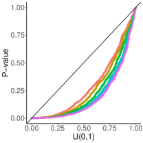
Figure 3: QQ plots of p๐‘p-values for changepoints obtained using binary segmentation: hโ„Žh is the window size and ฮด๐›ฟ\delta the size of the change in the model from which we simulate. In (a), p๐‘p-values from our method are plotted against theoretical quantiles from Uโ€‹(0,1)๐‘ˆ01U(0,1) for N=1,2,5,10,20,50๐‘125102050N=1,2,5,10,20,50. (b), (c) and (d) show QQ plots of p๐‘p-values calculated using our method (with N=2,5,10,20,50๐‘25102050N=2,5,10,20,50) against p๐‘p-values from the method of Jewell etย al., (2022) (equivalent to N=1๐‘1N=1).

In Section 3.3, we showed that our p๐‘p-value estimates were valid p๐‘p-values under H0subscript๐ป0H_{0}. In this section we show that, under H1subscript๐ป1H_{1}, our method has greater power to detect changepoints than that of Jewell etย al., (2022) for binary segmentation, and we investigate how the power changes with window size hโ„Žh, size of change ฮด๐›ฟ\delta, and number of samples N๐‘N. All simulations are conducted in R; the code is available at https://github.com/rachelcarrington/changepointsR.

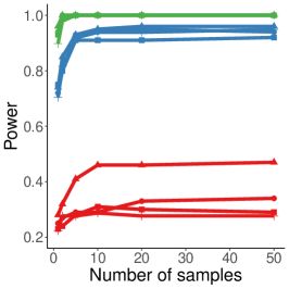
In each case, we set the number of data points T=1000๐‘‡1000T=1000, and take ฯƒ2=1superscript๐œŽ21\sigma^{2}=1. For Figures 3 and 4, we simulate from a model with a single change at t=500๐‘ก500t=500, where the change is of size ฮด๐›ฟ\delta: we consider ฮด=1,2,3๐›ฟ123\delta=1,2,3. In each case, we estimate changepoints using binary segmentation, and calculate the p๐‘p-value for the first detected changepoint. Simulations where the changepoint algorithm returns no changepoints are discarded. In Figure 5 we simulate from a model with 4 changes, at t=100,400,500,700๐‘ก100400500700t=100,400,500,700, and test for changes at the first 4 estimated changepoints.

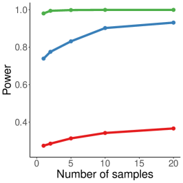
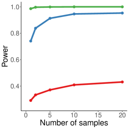
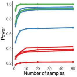
Figure 3 shows QQ plots of p๐‘p-values for binary segmentation, where we simulate data with a single change of size ฮด๐›ฟ\delta. Figure 3 (a) shows that our test has power when we simulate from H1subscript๐ป1H_{1}, and the power increases with the number of samples N๐‘N. In Figure 3 (b)-(d), p๐‘p-values from the method of Jewell etย al., (2022) (equivalent to N=1๐‘1N=1) are plotted against p๐‘p-values from our method with different values of N๐‘N. The p๐‘p-values generated from our method are generally smaller, indicating increased power, particularly so as hโ„Žh and ฮด๐›ฟ\delta increase. Figure 4 shows plots of the power for different values of hโ„Žh and ฮด๐›ฟ\delta: we see that initially increasing the number of Monte Carlo samples N๐‘N leads to substantial increases in power, but this levels off as N๐‘N continues to increase. Figure 5 shows the same thing when simulating from a model with 4 changepoints.
Refer to caption

h=10โ„Ž10h=10Refer to captionh=20โ„Ž20h=20Refer to captionh=50โ„Ž50h=50

Figure 4: Rejection rates of H0subscript๐ป0H_{0} for binary segmentation, plotted against N๐‘N. On each plot the three lines show the proportion of samples where the p๐‘p-value was below 0.050.050.05, leading H0subscript๐ป0H_{0} to be rejected. Each line corresponds to a different size of change ฮด๐›ฟ\delta: green corresponds to ฮด=3๐›ฟ3\delta=3, blue to ฮด=2๐›ฟ2\delta=2, and red to ฮด=1๐›ฟ1\delta=1.
Refer to caption

h=10โ„Ž10h=10Refer to captionh=20โ„Ž20h=20Refer to captionh=30โ„Ž30h=30

Figure 5: Rejection rates of H0subscript๐ป0H_{0} for different values of hโ„Žh, ฮด๐›ฟ\delta, and N๐‘N, when we simulate from a model with 4 changepoints, and apply binary segmentation with 4 changepoints. For each hโ„Žh, the process is run three times with changes of size ฮด=1,2,3๐›ฟ123\delta=1,2,3, which are shown on the plots as red, blue, and green lines respectively. Each line corresponds to a changepoint.

Further plots, which show similar results for wild binary segmentation and L0subscript๐ฟ0L_{0} segmentation, are given in Appendix B.1.

4.2 Multiple testing

We often detect multiple changepoints in a given data set, and as we conduct hypothesis tests at each estimated changepoint, we need to account for the fact that we carry out multiple tests. There are two common approaches to do so. One is to use a Bonferroni correction, or the Holm-Bonferroni method (Holm,, 1979). These provide control over the family wise error rate, i.e. the rate of one or more true null hypotheses, and do not make any assumptions on the dependence of the p๐‘p-values.

Alternatively we may wish to control the false discovery rate (FDR), the proportion of rejected null hypotheses that are true. This can be done using the Benjamini-Hochberg procedure (Benjamini and Hochberg,, 1995), but this procedure assumes independent p๐‘p-values. If we are testing the presence for a change in non-overlapping regions of the data, then the unconditional test-statistics are independent. However, the conditioning on the selection can induce dependence. We investigated empirically the level of dependence, see for example Appendix B.2, where we observed that there is non-zero but small positive correlation in p๐‘p-values (with e.g. correlation less than 0.050.050.05 across the scenarios). This suggests the use of Benjamini-Hochberg may be appropriate in practice, and below we consider both this and the Holm-Bonferroni method. For comparison, we also provide the false discovery rate we obtain using a MOSUM approach: for consistency we set the window sizes in each case to be the same, i.e. G=h๐บโ„ŽG=h.

Table 1 shows the number of false positives we get when we simulate from H0subscript๐ป0H_{0} with T=1000๐‘‡1000T=1000, and adjust the p๐‘p-values using the Holm-Bonferroni and Benjamini-Hochberg methods, for the method of (Jewell etย al.,, 2022) and our method; we also calculate this for MOSUM. In each case the mean number of false positives is below 0.050.050.05, suggesting that our tests are slightly conservative, although it is lower for MOSUM than for our method. Table 2 shows the mean number of true positives and the error rate (family-wise error rate for the Holm-Bonferroni method and false discovery rate for Benjamini-Hochberg) obtained when simulating under H1subscript๐ป1H_{1}, with K=1,4,9๐พ149K=1,4,9 equally spaced changepoints. A true positive occurs if a changepoint with p๐‘p-value below 0.05 is detected within the region (ฯ„โˆ’h,ฯ„+h)๐œโ„Ž๐œโ„Ž(\tau-h,\tau+h) for some ฯ„๐œ\tau in the set of true changepoints (we set h=10โ„Ž10h=10). Our method outperforms both that of Jewell etย al., (2022) and MOSUM at finding true changepoints. All three methods have very few false discoveries; our method has a lower false discovery rate than MOSUM when the true number of changepoints is small, although it is higher (but still small) when the true number of changepoints is higher. For binary segmentation, the error rate will depend in part on the changepoint threshold, which here we set to 3. This is a relatively high threshold, which means that most detected changepoints correspond to true changes, and hence the overall error rates are substantially below the 5% threshold. Appendix C shows results we obtain using different choices of threshold, as well as for different values of T๐‘‡T; these show similar numbers of true positives for a range of thresholds, whilst all having an error rate below 5%.

Table 1: Simulating from H0subscript๐ป0H_{0} with T=1000๐‘‡1000T=1000, we applied binary segmentation and MOSUM and calculated how many times H0subscript๐ป0H_{0} was falsely rejected. The table reports the mean number of estimated changepoints with adjusted p๐‘p-value below 0.05 across 1000 iterations, and the proportion of runs in which there was at least one false discovery, for both the Holm-Bonferroni and Benjamini-Hochberg procedures.
Mean false positives Proportion with โ‰ฅ1absent1\geq 1 false positive
H-B B-H H-B B-H
BS, N=1๐‘1N=1 0.03 0.03 0.03 0.03
BS, N=10๐‘10N=10 0.03 0.04 0.03 0.03
MOSUM 0.01 0.01
Table 2: Mean number of true positives and error rate when simulating from a model with T=1000๐‘‡1000T=1000 and K๐พK equally spaced changepoints, with ฮผ๐œ‡\mu alternating between 111 and โˆ’11-1, using binary segmentation and MOSUM. The error rate given is the family-wise error rate for the Holm-Bonferroni method, and the false discovery rate for the Benjamini-Hochberg method and for MOSUM. This is calculated as Fโ€‹Dโ€‹R=false positivesfalse positivesย +ย true positives๐น๐ท๐‘…false positivesfalse positivesย ย true positivesFDR=\frac{\text{false positives}}{\text{false positives }+\text{ true positives}}.
Mean true positives Error rate (%)
H-B B-H H-B B-H
BS, N=1๐‘1N=1 0.79 0.79 0.60 0.53
K=1๐พ1K=1 BS, N=10๐‘10N=10 0.94 0.94 0.50 0.29
MOSUM 0.58 1.20
BS, N=1๐‘1N=1 2.78 2.92 0.90 0.42
K=4๐พ4K=4 BS, N=10๐‘10N=10 3.42 3.51 1.50 0.46
MOSUM 2.32 0.22
BS, N=1๐‘1N=1 5.56 6.38 1.50 0.42
K=9๐พ9K=9 BS, N=10๐‘10N=10 7.23 7.80 2.10 0.51
MOSUM 5.30 0.09
Refer to caption
Refer to caption
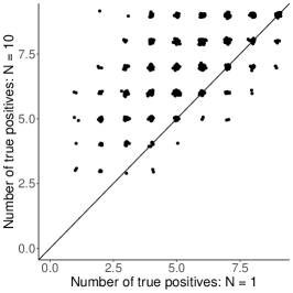
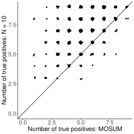
Figure 6: Plots showing the number of true positives found in 1000 simulations using our method with N=10๐‘10N=10 against the number found using the method of Jewell etย al., (2022) (left) and MOSUM (right). A small amount of noise has been added so that points corresponding to different simulated data sets can be distinguished.

Figure 6 shows plots of the number of true positives found using our method wit N=10๐‘10N=10, against the number of true positives found using N=1๐‘1N=1 (equivalent to the method of Jewell etย al., (2022)) and MOSUM, for each of 1000 simulations from a model with 9 true positives. A small amount of noise has been added to points to allow for visualisation. We see that in both cases, our method finds the same number or more true positives in most cases.

4.3 Robustness

We now investigate how well our method works if the assumptions that the noise in the data is i.i.d. and Gaussian with known variance, do not hold. To get some intuition it is helpful to consider which aspects of our test depend on the distributional assumptions. Our test is based on two parts: the first is the distribution of ฯ•italic-ฯ•\phi and ๐๐\boldsymbol{\psi} conditional on the data outside the region of our test and the mean of the data within the region; the second are, for each value of ๐๐\boldsymbol{\psi}, the set of ฯ•italic-ฯ•\phi values that would lead to the same information used to choose the test. It is only the first part that depends on the distributional assumptions. If these do not hold then our test statistic has a different distribution but truncated to the same range of values for each ๐๐\boldsymbol{\psi}.

Refer to caption

H0subscript๐ป0H_{0}Refer to captionH1,ฮด=2subscript๐ป1๐›ฟ2H_{1},\delta=2

Figure 7: QQ plots of p๐‘p-values when ฯƒ2superscript๐œŽ2\sigma^{2} is estimated using median absolute deviation, rather than being assumed known. In each case T=1000๐‘‡1000T=1000 and h=10โ„Ž10h=10 and we estimate 1 changepoint using binary segmentation and calculate the associated p๐‘p-value. In the left-hand plot we simulate from H0subscript๐ป0H_{0} with no changes; in the right-hand plot we simulate from a model with a single change of size ฮด=2๐›ฟ2\delta=2 at ฯ„=500๐œ500\tau=500.

Thus in situations where we have a limiting regime whereby the distribution of ฯ•italic-ฯ•\phi and ๐๐\boldsymbol{\psi} converge to their assumed distribution, our method will give asymptotically correct p๐‘p-values. The most important example of this is where the independent Gaussian assumption for the noise is correct but the variance is unknown. In this case if we use any consistent (in data size T๐‘‡T) estimator for the variance, our approach will be asymptotically valid as Tโ†’โˆžโ†’๐‘‡T\rightarrow\infty (see Jewell etย al.,, 2022).

We investigated the finite sample performance, with Figure 7 showing QQ plots of the p๐‘p-values obtained when we simulate from a model with no changepoints (left) and with one changepoint (right), apply binary segmentation with one changepoint, and estimate the variance of ๐‘ฟ๐‘ฟ\boldsymbol{X} using median absolute deviation. We see that the distribution of p๐‘p-values under H0subscript๐ป0H_{0} is very close to Uโ€‹(0,1)๐‘ˆ01U(0,1), and under H1subscript๐ป1H_{1} the distribution is close to that when we assume known variance (compare with Figure 3d).
Refer to caption

(a)H0subscript๐ป0H_{0}, ฮฝ=5๐œˆ5\nu=5Refer to caption(b)H0subscript๐ป0H_{0}, ฮฝ=10๐œˆ10\nu=10Refer to caption(c)H1subscript๐ป1H_{1}, ฮฝ=5๐œˆ5\nu=5, ฮด=1๐›ฟ1\delta=1

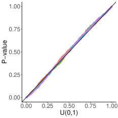
Figure 8: QQ plots of p๐‘p-values obtained when simulating from a tฮฝsubscript๐‘ก๐œˆt_{\nu} distribution with ฮฝ๐œˆ\nu degrees of freedom.

The discussion above suggests that our approach may also be appropriate in situations where a central limit theorem holds for our test statistic, so that a Gaussian approximation for the distribution of ฯ•italic-ฯ•\phi is reasonable. To investigate this, we simulate data ๐‘ฟ๐‘ฟ\boldsymbol{X} with heavy-tailed noise, simulating from a studentโ€™s t๐‘กt distribution. Figure 8 shows QQ plots we obtain when data is simulated from a tฮฝsubscript๐‘ก๐œˆt_{\nu} distribution with ฮฝ=5,10๐œˆ510\nu=5,10 degrees of freedom. In panels (a) and (b) we simulate from H0subscript๐ป0H_{0} and find that the p๐‘p-values approximately follow the expected distribution Uโ€‹(0,1)๐‘ˆ01U(0,1). In panel (c) we simulate data with a single change of size ฮด=1๐›ฟ1\delta=1; in this case the p๐‘p-values are smaller than under H0subscript๐ป0H_{0}, so the test has power to detect deviation from H0subscript๐ป0H_{0}. Figure 14 in Appendix B.3 shows similar results when we simulate ๐‘ฟ๐‘ฟ\boldsymbol{X} with Laplace noise.

5 Application to genomic data

Refer to caption
Refer to caption
Figure 9: Estimated changepoints in GC content data. Binary segmentation was used to estimate 38 changepoints, and we set h=10โ„Ž10h=10. Each vertical line corresponds to an estimated changepoint; changepoints found to be significant at significance level ฮฑ=0.05๐›ผ0.05\alpha=0.05 are shown in red, with others shown in grey. In the top panel, we used N=1๐‘1N=1 (equivalent to the method of Jewell etย al., (2022)) to calculate p๐‘p-values; in the bottom panel, we used N=10๐‘10N=10.

We now apply our method to genomic data consisting of GC content in 3kb windows along the human chromosome, using both binary segmentation and L0subscript๐ฟ0L_{0} segmentation. The data is available in the R package changepoint. As in Jewell etย al., (2022), only the first 200020002000 data points are used, and we set the detection thresholds so that the number of changepoints detected is 38. For each changepoint, we calculate a p๐‘p-value using both the method of Jewell etย al., (2022) (equivalent to our method with N=1๐‘1N=1) and our method (with N=10๐‘10N=10 and N=20๐‘20N=20), using a window size of h=10โ„Ž10h=10. The variance of the data is estimated using median absolute deviation. Figure 9 shows plots of the data and estimated changepoints for binary segmentation, where red lines correspond to estimated changepoints with p๐‘p-values smaller than 0.050.050.05 (after controlling for multiple testing by using the Holm-Bonferroni correction), and grey lines to changepoints with p๐‘p-values above 0.050.050.05. The corresponding figure for L0subscript๐ฟ0L_{0} segmentation is included in Appendix B.1. In both cases, a greater proportion of changepoints are deemed to be significant using our method, indicating that it has greater power to detect changes.

Table 3 gives the number of significant changepoints found in each case. To account for the fact that we are conducting multiple tests, we report results after controlling for multiple testing using the Holm-Bonferroni and Benjamini-Hochberg procedures. For both binary segmentation and L0subscript๐ฟ0L_{0} segmentation, we get a greater number of significant changepoints when N=10๐‘10N=10 than when N=1๐‘1N=1, although increasing N๐‘N beyond this does not yield much further improvement. Hence, in practice, only a moderate number of Monte Carlo samples is sufficient to get an increase in power.

Interestingly for this application the MOSUM approach finds more significant changepoints, with 45 changes with a p๐‘p-value less than 0.05. This may be due to binary segmentation or L0subscript๐ฟ0L_{0} penalisation approaches detecting too few changes.

Table 3: Number of changepoints in GC content data with p๐‘p-values below ฮฑ=0.05๐›ผ0.05\alpha=0.05, where we control for multiple testing using the Holm-Bonferroni and Benjamini-Hochberg methods. We implement our method with binary segmentation and L0subscript๐ฟ0L_{0} segmentation, where N=1๐‘1N=1 is equivalent to the method of Jewell etย al., (2022).
Number of p๐‘p-values <0.05absent0.05<0.05
Changepoint algorithm Holm-Bonferroni Benjamini-Hochberg
N=1๐‘1N=1 15 21
Binary segmentation, K=38๐พ38K=38 N=10๐‘10N=10 27 30
N=20๐‘20N=20 27 30
N=1๐‘1N=1 20 26
Binary segmentation, K=45๐พ45K=45 N=10๐‘10N=10 32 36
N=20๐‘20N=20 31 36
N=1๐‘1N=1 16 25
L0subscript๐ฟ0L_{0} segmentation, K=38๐พ38K=38 N=10๐‘10N=10 25 28
N=20๐‘20N=20 28 29
N=1๐‘1N=1 20 27
L0subscript๐ฟ0L_{0} segmentation, K=46๐พ46K=46 N=10๐‘10N=10 26 32
N=20๐‘20N=20 27 32

6 Discussion

We have introduced a method for increasing the power of changepoint inference procedures, by reducing the amount of information we condition on. We have shown that this method is effective in increasing power compared to existing methods, both in simulated and real-world data sets.

Whilst our approach has been developed for changepoint problems, the general idea can be applied to other scenarios such as clustering Gao etย al., (2022); Chen and Witten, (2023) or regression tress Neufeld etย al., (2022). For example, current methods for post-selection inference after clustering are based on a test statistic that compares the mean of the cluster, and fixes the projection of the data that is orthogonal to this. However we could reduce this to conditioning just on the sample mean of one of the clusters, and the data in the clusters that are not being combined. Our method would then re-simulate the perturbations of each data point about its clustered mean, apply the existing post-selection inference method to each data set, and calculate the weighted average as we do in this paper. We believe that this approach would have similar properties, of being a valid p๐‘p-value regardless of the Monte Carlo sample size, and of having larger power as the Monte Carlo sample size increases. Our approach for constructing valid p๐‘p-values when using Monte Carlo to estimate post-selection p๐‘p-values (e.g. Saha etย al.,, 2022) may also be applicable more widely.

Acknowledgement

This work is supported by EPSRC grant number EP/V053590/1.

References

  • Aston and Kirch, (2012) Aston, J.ย A. and Kirch, C. (2012). Evaluating stationarity via change-point alternatives with applications to fMRI data. The Annals of Applied Statistics, 6(4):1906โ€“1948.
  • Baranowski etย al., (2019) Baranowski, R., Chen, Y., and Fryzlewicz, P. (2019). Narrowest-over-threshold detection of multiple change points and change-point-like features. Journal of the Royal Statistical Society: Series B, 81(3):649โ€“672.
  • Barrett etย al., (2017) Barrett, E., Bolz-Tereick, C.ย F., Killick, R., Mount, S., and Tratt, L. (2017). Virtual machine warmup blows hot and cold. Proceedings of the ACM on Programming Languages, 1(OOPSLA):1โ€“27.
  • Benjamini and Hochberg, (1995) Benjamini, Y. and Hochberg, Y. (1995). Controlling the false discovery rate: a practical and powerful approach to multiple testing. Journal of the Royal Statistical Society: Series B, 57(1):289โ€“300.
  • Berk etย al., (2013) Berk, R., Brown, L., Buja, A., Zhang, K., and Zhao, L. (2013). Valid post-selection inference. The Annals of Statistics, 41:802โ€“837.
  • Braun etย al., (2000) Braun, J.ย V., Braun, R., and Mรผller, H.-G. (2000). Multiple changepoint fitting via quasilikelihood, with application to DNA sequence segmentation. Biometrika, 87(2):301โ€“314.
  • Chen etย al., (2023) Chen, Y.ย T., Jewell, S.ย W., and Witten, D.ย M. (2023). Quantifying uncertainty in spikes estimated from calcium imaging data. Biostatistics, 24(2):481โ€“501.
  • Chen and Witten, (2023) Chen, Y.ย T. and Witten, D.ย M. (2023). Selective inference for k-means clustering. Journal of Machine Learning Research, 24(152):1โ€“41.
  • Dubey and Mรผller, (2020) Dubey, P. and Mรผller, H.-G. (2020). Frรฉchet change-point detection. The Annals of Statistics, 48(6):3312โ€“3335.
  • Duy and Takeuchi, (2022) Duy, V. N.ย L. and Takeuchi, I. (2022). More powerful conditional selective inference for generalized lasso by parametric programming. The Journal of Machine Learning Research, 23(1):13544โ€“13580.
  • Duy etย al., (2020) Duy, V. N.ย L., Toda, H., Sugiyama, R., and Takeuchi, I. (2020). Computing valid p-value for optimal changepoint by selective inference using dynamic programming. Advances in Neural Information Processing Systems, 33:11356โ€“11367.
  • Eichinger and Kirch, (2018) Eichinger, B. and Kirch, C. (2018). A MOSUM procedure for the estimation of multiple random change points. Bernoulli, 24(1):526โ€“564.
  • Fang etย al., (2020) Fang, X., Li, J., and Siegmund, D. (2020). Segmentation and estimation of change-point models: false positive control and confidence regions. The Annals of Statistics, 48(3):1615โ€“1647.
  • Fearnhead, (2006) Fearnhead, P. (2006). Exact and efficient Bayesian inference for multiple changepoint problems. Statistics and Computing, 16(2):203โ€“213.
  • Fearnhead and Fryzlewicz, (2022) Fearnhead, P. and Fryzlewicz, P. (2022). Detecting a single change-point. arXiv preprint arXiv:2210.07066.
  • Fearnhead and Rigaill, (2019) Fearnhead, P. and Rigaill, G. (2019). Changepoint detection in the presence of outliers. Journal of the American Statistical Association, 114(525):169โ€“183.
  • Fearnhead and Rigaill, (2020) Fearnhead, P. and Rigaill, G. (2020). Relating and comparing methods for detecting changes in mean. Stat, 9(1):e291.
  • Fithian etย al., (2014) Fithian, W., Sun, D., and Taylor, J. (2014). Optimal inference after model selection. arXiv:1410.2597.
  • Frick etย al., (2014) Frick, K., Munk, A., and Sieling, H. (2014). Multiscale change point inference. Journal of the Royal Statistical Society: Series B, 76(3):495โ€“580.
  • Fryzlewicz, (2014) Fryzlewicz, P. (2014). Wild binary segmentation for multiple change-point detection. The Annals of Statistics, 42(6):2243โ€“2281.
  • Fryzlewicz, (2021) Fryzlewicz, P. (2021). Robust narrowest significance pursuit: inference for multiple change-points in the median. arXiv:2109.02487.
  • Fryzlewicz, (2023) Fryzlewicz, P. (2023). Narrowest significance pursuit: inference for multiple change-points in linear models. Journal of the American Statistical Association, pages 1โ€“14.
  • Gao etย al., (2022) Gao, L.ย L., Bien, J., and Witten, D. (2022). Selective inference for hierarchical clustering. Journal of the American Statistical Association, pages 1โ€“11.
  • Hao etย al., (2013) Hao, N., Niu, Y.ย S., and Zhang, H. (2013). Multiple change-point detection via a screening and ranking algorithm. Statistica Sinica, 23(4):1553.
  • Heard and Turcotte, (2014) Heard, N.ย A. and Turcotte, M.ย J. (2014). Monitoring a device in a communication network. In Data Analysis for Network Cyber-security, pages 151โ€“188. World Scientific.
  • Holm, (1979) Holm, S. (1979). A simple sequentially rejective multiple test procedure. Scandinavian Journal of Statistics, pages 65โ€“70.
  • Hyun etย al., (2018) Hyun, S., Gโ€™Sell, M., and Tibshirani, R.ย J. (2018). Exact post-selection inference for the generalized lasso path. Electronic Journal of Statistics, 12(1):1053โ€“1097.
  • Hyun etย al., (2021) Hyun, S., Lin, K.ย Z., Gโ€™Sell, M., and Tibshirani, R.ย J. (2021). Post-selection inference for changepoint detection algorithms with application to copy number variation data. Biometrics, 77(3):1037โ€“1049.
  • Jewell etย al., (2022) Jewell, S., Fearnhead, P., and Witten, D. (2022). Testing for a change in mean after changepoint detection. Journal of the Royal Statistical Society: Series B, 84(4):1082โ€“1104.
  • Jewell etย al., (2020) Jewell, S.ย W., Hocking, T.ย D., Fearnhead, P., and Witten, D.ย M. (2020). Fast nonconvex deconvolution of calcium imaging data. Biostatistics, 21(4):709โ€“726.
  • Killick etย al., (2012) Killick, R., Fearnhead, P., and Eckley, I.ย A. (2012). Optimal detection of changepoints with a linear computational cost. Journal of the American Statistical Association, 107(500):1590โ€“1598.
  • Kim etย al., (2009) Kim, S.-J., Koh, K., Boyd, S., and Gorinevsky, D. (2009). l1subscript๐‘™1l_{1} trend filtering. SIAM review, 51(2):339โ€“360.
  • Kuchibhotla etย al., (2022) Kuchibhotla, A.ย K., Kolassa, J.ย E., and Kuffner, T.ย A. (2022). Post-selection inference. Annual Review of Statistics and Its Application, 9:505โ€“527.
  • Li etย al., (2016) Li, H., Munk, A., and Sieling, H. (2016). FDR-control in multiscale change-point segmentation. Electronic Journal of Statistics, 10(1):918โ€“959.
  • Liu etย al., (2018) Liu, K., Markovic, J., and Tibshirani, R. (2018). More powerful post-selection inference, with application to the lasso. arXiv:1801.09037.
  • Maidstone etย al., (2017) Maidstone, R., Hocking, T., Rigaill, G., and Fearnhead, P. (2017). On optimal multiple changepoint algorithms for large data. Statistics and Computing, 27(2):519โ€“533.
  • Maleki etย al., (2016) Maleki, S., Bingham, C., and Zhang, Y. (2016). Development and realization of changepoint analysis for the detection of emerging faults on industrial systems. IEEE Transactions on Industrial Informatics, 12(3):1180โ€“1187.
  • Meier etย al., (2021) Meier, A., Kirch, C., and Cho, H. (2021). mosum: A package for moving sums in change-point analysis. Journal of Statistical Software, 97:1โ€“42.
  • Neufeld etย al., (2022) Neufeld, A.ย C., Gao, L.ย L., and Witten, D.ย M. (2022). Tree-values: selective inference for regression trees. Journal of Machine Learning Research, 23(305):1โ€“43.
  • Olshen etย al., (2004) Olshen, A.ย B., Venkatraman, E.ย S., Lucito, R., and Wigler, M. (2004). Circular binary segmentation for the analysis of array-based DNA copy number data. Biostatistics, 5(4):557โ€“572.
  • Pein etย al., (2017) Pein, F., Sieling, H., and Munk, A. (2017). Heterogeneous change point inference. Journal of the Royal Statistical Society: Series B, 79(4):1207โ€“1227.
  • Reeves etย al., (2007) Reeves, J., Chen, J., Wang, X.ย L., Lund, R., and Lu, Q.ย Q. (2007). A review and comparison of changepoint detection techniques for climate data. Journal of Applied Meteorology and Climatology, 46(6):900โ€“915.
  • Rinaldo etย al., (2019) Rinaldo, A., Wasserman, L., and Gโ€™Sell, M. (2019). Bootstrapping and sample splitting for high-dimensional, assumption-lean inference. The Annals of Statistics, 47(6):3438โ€“3469.
  • Saha etย al., (2022) Saha, A., Witten, D., and Bien, J. (2022). Inferring independent sets of Gaussian variables after thresholding correlations. arXiv:2211.01521.
  • Scott and Knott, (1974) Scott, A.ย J. and Knott, M. (1974). A cluster analysis method for grouping means in the analysis of variance. Biometrics, 30:507โ€“512.
  • (46) Shi, X., Beaulieu, C., Killick, R., and Lund, R. (2022a). Changepoint detection: An analysis of the central England temperature series. Journal of Climate, 35(19):2729โ€“2742.
  • (47) Shi, X., Gallagher, C., Lund, R., and Killick, R. (2022b). A comparison of single and multiple changepoint techniques for time series data. Computational Statistics & Data Analysis, 170:107433.
  • Song and Chen, (2022) Song, H. and Chen, H. (2022). Asymptotic distribution-free changepoint detection for data with repeated observations. Biometrika, 109(3):783โ€“798.
  • Tibshirani etย al., (2005) Tibshirani, R., Saunders, M., Rosset, S., Zhu, J., and Knight, K. (2005). Sparsity and smoothness via the fused lasso. Journal of the Royal Statistical Society: Series B, 67(1):91โ€“108.
  • Tibshirani, (2014) Tibshirani, R.ย J. (2014). Adaptive piecewise polynomial estimation via trend filtering. The Annals of Statistics, 42(1):285โ€“323.
  • Truong etย al., (2020) Truong, C., Oudre, L., and Vayatis, N. (2020). Selective review of offline change point detection methods. Signal Processing, 167:107299.
  • Wang etย al., (2021) Wang, D., Yu, Y., and Rinaldo, A. (2021). Optimal change point detection and localization in sparse dynamic networks. The Annals of Statistics, 49(1):203โ€“232.
  • Wang and Samworth, (2018) Wang, T. and Samworth, R.ย J. (2018). High dimensional change point estimation via sparse projection. Journal of the Royal Statistical Society: Series B, 80(1):57โ€“83.
  • Zhao etย al., (2021) Zhao, S., Witten, D., and Shojaie, A. (2021). In defense of the indefensible: A very naive approach to high-dimensional inference. Statistical Science, 36(4):562โ€“577.
  • Zhao etย al., (2022) Zhao, Z., Jiang, F., and Shao, X. (2022). Segmenting time series via self-normalisation. Journal of the Royal Statistical Society: Series B, 84(5):1699โ€“1725.

Appendix A Proofs

A.1 Proof of Theorem 1

Proof.

Fix ฮฑ๐›ผ\alpha, and consider maximising Prโก(Pโˆ—โ‰คฮฑ)Prsuperscript๐‘ƒ๐›ผ\Pr(P^{*}\leq\alpha). This corresponds to choosing a rejection region Rฮฑsubscript๐‘…๐›ผR_{\alpha} for (ฯ•,๐)italic-ฯ•๐(\phi,\boldsymbol{\psi}) that maximises

โˆซRฮฑk~โ€‹(|ฯ•|)โ€‹fโ€‹(ฯ•)โ€‹โˆi=12โ€‹hโˆ’2gโ€‹(ฯˆi)โ€‹dโ€‹ฯ•โ€‹dโ€‹๐,subscriptsubscript๐‘…๐›ผ~๐‘˜italic-ฯ•๐‘“italic-ฯ•superscriptsubscriptproduct๐‘–12โ„Ž2๐‘”subscript๐œ“๐‘–ditalic-ฯ•d๐\int_{R_{\alpha}}\tilde{k}(|\phi|)f(\phi)\prod_{i=1}^{2h-2}g(\psi_{i})\mbox{d}\phi\mbox{d}\boldsymbol{\psi},

subject to

โˆซRฮฑfโ€‹(ฯ•)โ€‹โˆi=12โ€‹hโˆ’2gโ€‹(ฯˆi)โ€‹dโ€‹ฯ•โ€‹dโ€‹๐โ‰คฮฑโ€‹โˆซ๐’ฎfโ€‹(ฯ•)โ€‹โˆi=12โ€‹hโˆ’2gโ€‹(ฯˆi)โ€‹dโ€‹ฯ•โ€‹dโ€‹๐.subscriptsubscript๐‘…๐›ผ๐‘“italic-ฯ•superscriptsubscriptproduct๐‘–12โ„Ž2๐‘”subscript๐œ“๐‘–ditalic-ฯ•d๐๐›ผsubscript๐’ฎ๐‘“italic-ฯ•superscriptsubscriptproduct๐‘–12โ„Ž2๐‘”subscript๐œ“๐‘–ditalic-ฯ•d๐\int_{R_{\alpha}}f(\phi)\prod_{i=1}^{2h-2}g(\psi_{i})\mbox{d}\phi\mbox{d}\boldsymbol{\psi}\leq\alpha\int_{\mathcal{S}}f(\phi)\prod_{i=1}^{2h-2}g(\psi_{i})\mbox{d}\phi\mbox{d}\boldsymbol{\psi}.

As k~~๐‘˜\tilde{k} is an increasing function of ฯ•italic-ฯ•\phi, it is straightforward that this is achieved for the region

Rฮฑ={(ฯ•,๐):|ฯ•|โ‰ฅcฮฑ},subscript๐‘…๐›ผconditional-setitalic-ฯ•๐italic-ฯ•subscript๐‘๐›ผR_{\alpha}=\{(\phi,\boldsymbol{\psi}):|\phi|\geq c_{\alpha}\},

with cฮฑsubscript๐‘๐›ผc_{\alpha} defined by

โˆซRฮฑfโ€‹(ฯ•)โ€‹โˆi=12โ€‹hโˆ’2gโ€‹(ฯˆi)โ€‹dโ€‹ฯ•โ€‹dโ€‹๐=ฮฑโ€‹โˆซ๐’ฎfโ€‹(ฯ•)โ€‹โˆi=12โ€‹hโˆ’2gโ€‹(ฯˆi)โ€‹dโ€‹ฯ•โ€‹dโ€‹๐.subscriptsubscript๐‘…๐›ผ๐‘“italic-ฯ•superscriptsubscriptproduct๐‘–12โ„Ž2๐‘”subscript๐œ“๐‘–ditalic-ฯ•d๐๐›ผsubscript๐’ฎ๐‘“italic-ฯ•superscriptsubscriptproduct๐‘–12โ„Ž2๐‘”subscript๐œ“๐‘–ditalic-ฯ•d๐\int_{R_{\alpha}}f(\phi)\prod_{i=1}^{2h-2}g(\psi_{i})\mbox{d}\phi\mbox{d}\boldsymbol{\psi}=\alpha\int_{\mathcal{S}}f(\phi)\prod_{i=1}^{2h-2}g(\psi_{i})\mbox{d}\phi\mbox{d}\boldsymbol{\psi}.

This is precisely the form of PIsubscript๐‘ƒ๐ผP_{I}, as PIโ‰คฮฑsubscript๐‘ƒ๐ผ๐›ผP_{I}\leq\alpha corresponds to |ฯ•|โ‰ฅcฮฑitalic-ฯ•subscript๐‘๐›ผ|\phi|\geq c_{\alpha}. The result follows directly.

We now show that the condition of the theorem holds if under the alternative the we have a common mean for Xฯ„^โˆ’h+1,โ€ฆ,Xฯ„^subscript๐‘‹^๐œโ„Ž1โ€ฆsubscript๐‘‹^๐œX_{\hat{\tau}-h+1},\ldots,X_{\hat{\tau}}, and a different common mean for Xฯ„^+1,โ€ฆ,Xฯ„^+hsubscript๐‘‹^๐œ1โ€ฆsubscript๐‘‹^๐œโ„ŽX_{\hat{\tau}+1},\ldots,X_{\hat{\tau}+h}, and that the density for the difference in means is symmetric about 0. Under this model, denote the difference in means at ฯ„^^๐œ\hat{\tau} by Y๐‘ŒY, and denotes its density function by hโ€‹(y)โ„Ž๐‘ฆh(y), which by assumption is symmetric about 00. First note that for this model ฯ•italic-ฯ•\phi is independent of ๐1:2โ€‹hโˆ’2subscript๐:12โ„Ž2\boldsymbol{\psi}_{1:2h-2} as the covariance of (ฯ•,๐1:2โ€‹hโˆ’2)italic-ฯ•subscript๐:12โ„Ž2(\phi,\boldsymbol{\psi}_{1:2h-2}) is still diagonal, and it is straightforward to hence show that the conditional distribution of ๐1:2โ€‹hโˆ’2subscript๐:12โ„Ž2\boldsymbol{\psi}_{1:2h-2} given ฯ•italic-ฯ•\phi is unchanged. So we need just check the condition on the marginal distribution for ฯ•italic-ฯ•\phi.

Under H1subscript๐ป1H_{1},

ฯ•|YโˆผNโ€‹(Y,โ€–๐‚ฯ„^โ€–22โ€‹ฯƒ2).similar-toconditionalitalic-ฯ•๐‘Œ๐‘๐‘Œsuperscriptsubscriptnormsubscript๐‚^๐œ22superscript๐œŽ2\phi|Y\sim N(Y,||\boldsymbol{\nu}_{\hat{\tau}}||_{2}^{2}\sigma^{2}).

and hence

fH1โ€‹(ฯ•)=โˆซYfH1โ€‹(ฯ•|y)โ€‹hโ€‹(y)โ€‹๐‘‘y,subscript๐‘“subscript๐ป1italic-ฯ•subscript๐‘Œsubscript๐‘“subscript๐ป1conditionalitalic-ฯ•๐‘ฆโ„Ž๐‘ฆdifferential-d๐‘ฆf_{H_{1}}(\phi)=\int_{Y}f_{H_{1}}(\phi|y)h(y)dy,

where fH1subscript๐‘“subscript๐ป1f_{H_{1}} denotes the density of ฯ•italic-ฯ•\phi under H1subscript๐ป1H_{1}. Since hโ„Žh is symmetric in Y๐‘ŒY, we get

hโ€‹(ฯ•)=โˆซYfH1โ€‹(ฯ•|y)โ€‹hโ€‹(y)โ€‹๐‘‘y=โˆซY>0fH1โ€‹(ฯ•|y)โ€‹hโ€‹(y)โ€‹๐‘‘y+โˆซY<0fH1โ€‹(ฯ•|y)โ€‹hโ€‹(y)โ€‹๐‘‘y=โˆซY>0(fH1โ€‹(ฯ•|y)+fH1โ€‹(ฯ•|โˆ’y))โ€‹hโ€‹(y)โ€‹๐‘‘y.โ„Žitalic-ฯ•subscript๐‘Œsubscript๐‘“subscript๐ป1conditionalitalic-ฯ•๐‘ฆโ„Ž๐‘ฆdifferential-d๐‘ฆsubscript๐‘Œ0subscript๐‘“subscript๐ป1conditionalitalic-ฯ•๐‘ฆโ„Ž๐‘ฆdifferential-d๐‘ฆsubscript๐‘Œ0subscript๐‘“subscript๐ป1conditionalitalic-ฯ•๐‘ฆโ„Ž๐‘ฆdifferential-d๐‘ฆsubscript๐‘Œ0subscript๐‘“subscript๐ป1conditionalitalic-ฯ•๐‘ฆsubscript๐‘“subscript๐ป1conditionalitalic-ฯ•๐‘ฆโ„Ž๐‘ฆdifferential-d๐‘ฆ\begin{split}h(\phi)&=\int_{Y}f_{H_{1}}(\phi|y)h(y)dy\\ &=\int_{Y>0}f_{H_{1}}(\phi|y)h(y)dy+\int_{Y<0}f_{H_{1}}(\phi|y)h(y)dy\\ &=\int_{Y>0}\left(f_{H_{1}}(\phi|y)+f_{H_{1}}(\phi|-y)\right)h(y)dy.\end{split}

Note that fH1โ€‹(ฯ•|y)=fH1โ€‹(ฯ•โˆ’y|0)=fโ€‹(ฯ•โˆ’y)subscript๐‘“subscript๐ป1conditionalitalic-ฯ•๐‘ฆsubscript๐‘“subscript๐ป1italic-ฯ•conditional๐‘ฆ0๐‘“italic-ฯ•๐‘ฆf_{H_{1}}(\phi|y)=f_{H_{1}}(\phi-y|0)=f(\phi-y), so

fH1โ€‹(ฯ•)=โˆซY>0(fโ€‹(ฯ•โˆ’y)+fโ€‹(ฯ•+y))โ€‹hโ€‹(y)โ€‹๐‘‘y,subscript๐‘“subscript๐ป1italic-ฯ•subscript๐‘Œ0๐‘“italic-ฯ•๐‘ฆ๐‘“italic-ฯ•๐‘ฆโ„Ž๐‘ฆdifferential-d๐‘ฆf_{H_{1}}(\phi)=\int_{Y>0}\left(f(\phi-y)+f(\phi+y)\right)h(y)dy,

and so

kโ€‹(ฯ•)=โˆซY>0(fโ€‹(ฯ•โˆ’y)+fโ€‹(ฯ•+y))โ€‹hโ€‹(y)โ€‹๐‘‘yfโ€‹(ฯ•)=โˆซY>0fโ€‹(ฯ•โˆ’y)+fโ€‹(ฯ•+y)fโ€‹(ฯ•)โ€‹hโ€‹(y)โ€‹๐‘‘y.๐‘˜italic-ฯ•subscript๐‘Œ0๐‘“italic-ฯ•๐‘ฆ๐‘“italic-ฯ•๐‘ฆโ„Ž๐‘ฆdifferential-d๐‘ฆ๐‘“italic-ฯ•subscript๐‘Œ0๐‘“italic-ฯ•๐‘ฆ๐‘“italic-ฯ•๐‘ฆ๐‘“italic-ฯ•โ„Ž๐‘ฆdifferential-d๐‘ฆk(\phi)=\frac{\int_{Y>0}\left(f(\phi-y)+f(\phi+y)\right)h(y)dy}{f(\phi)}=\int_{Y>0}\frac{f(\phi-y)+f(\phi+y)}{f(\phi)}h(y)dy.

Let

k~โ€‹(ฯ•)=fโ€‹(ฯ•โˆ’y)+fโ€‹(ฯ•+y)fโ€‹(ฯ•)=eโˆ’(ฯ•โˆ’y)2/2โ€‹โ€–๐‚ฯ„^โ€–22โ€‹ฯƒ2+eโˆ’(ฯ•+y)2/2โ€‹โ€–๐‚ฯ„^โ€–22โ€‹ฯƒ2eโˆ’ฯ•2/2โ€‹โ€–๐‚ฯ„^โ€–22โ€‹ฯƒ2=eโˆ’y2/2โ€‹โ€–๐‚ฯ„^โ€–22โ€‹ฯƒ2โ€‹(eฯ•โ€‹y/2โ€‹โ€–๐‚ฯ„^โ€–22โ€‹ฯƒ2โˆ’eโˆ’ฯ•โ€‹y/2โ€‹โ€–๐‚ฯ„^โ€–22โ€‹ฯƒ2).~๐‘˜italic-ฯ•๐‘“italic-ฯ•๐‘ฆ๐‘“italic-ฯ•๐‘ฆ๐‘“italic-ฯ•superscript๐‘’superscriptitalic-ฯ•๐‘ฆ22superscriptsubscriptnormsubscript๐‚^๐œ22superscript๐œŽ2superscript๐‘’superscriptitalic-ฯ•๐‘ฆ22superscriptsubscriptnormsubscript๐‚^๐œ22superscript๐œŽ2superscript๐‘’superscriptitalic-ฯ•22superscriptsubscriptnormsubscript๐‚^๐œ22superscript๐œŽ2superscript๐‘’superscript๐‘ฆ22superscriptsubscriptnormsubscript๐‚^๐œ22superscript๐œŽ2superscript๐‘’italic-ฯ•๐‘ฆ2superscriptsubscriptnormsubscript๐‚^๐œ22superscript๐œŽ2superscript๐‘’italic-ฯ•๐‘ฆ2superscriptsubscriptnormsubscript๐‚^๐œ22superscript๐œŽ2\begin{split}\tilde{k}(\phi)&=\frac{f(\phi-y)+f(\phi+y)}{f(\phi)}\\ &=\frac{e^{-(\phi-y)^{2}/2||\boldsymbol{\nu}_{\hat{\tau}}||_{2}^{2}\sigma^{2}}+e^{-(\phi+y)^{2}/2||\boldsymbol{\nu}_{\hat{\tau}}||_{2}^{2}\sigma^{2}}}{e^{-\phi^{2}/2||\boldsymbol{\nu}_{\hat{\tau}}||_{2}^{2}\sigma^{2}}}\\ &=e^{-y^{2}/2||\boldsymbol{\nu}_{\hat{\tau}}||_{2}^{2}\sigma^{2}}\left(e^{\phi y/2||\boldsymbol{\nu}_{\hat{\tau}}||_{2}^{2}\sigma^{2}}-e^{-\phi y/2||\boldsymbol{\nu}_{\hat{\tau}}||_{2}^{2}\sigma^{2}}\right).\end{split}

This is monotone increasing in |ฯ•|italic-ฯ•|\phi| for every y>0๐‘ฆ0y>0. Therefore, this must also be true of kโ€‹(ฯ•)๐‘˜italic-ฯ•k(\phi). โˆŽ

A.2 Proof of Theorem 2

Proof.

The p๐‘p-value, p^Nsubscript^๐‘๐‘\hat{p}_{N}, is invariant to shuffling the labels of the ๐(j)superscript๐๐‘—\boldsymbol{\psi}^{(j)}s. Let ๐(1:N)superscript๐:1๐‘\boldsymbol{\psi}^{(1:N)} denote the set of ๐(j)superscript๐๐‘—\boldsymbol{\psi}^{(j)} values after shuffling, and I๐ผI the label of ๐(j)superscript๐๐‘—\boldsymbol{\psi}^{(j)} that corresponds to the observed data.

The proof follows by calculating Prโก(p^N>ฮฑ|๐(1:N))Prsubscript^๐‘๐‘conditional๐›ผsuperscript๐:1๐‘\Pr(\hat{p}_{N}>\alpha|\boldsymbol{\psi}^{(1:N)}). This requires calculating the distribution of ฯ•italic-ฯ•\phi given ๐(1:N)superscript๐:1๐‘\boldsymbol{\psi}^{(1:N)}.

As before, let f๐‘“f and g๐‘”g represent the pdfs under the null of ฯ•italic-ฯ•\phi and each component of ๐๐\boldsymbol{\psi}, respectively. Then

fโ€‹(ฯ•,๐(1:N),I|๐’ฎ)โˆfโ€‹(ฯ•)โ€‹(โˆi=1Ngโ€‹(๐(i)))โ€‹๐•€{ฯ•โˆˆ๐’ฎ๐(I)}.proportional-to๐‘“italic-ฯ•superscript๐:1๐‘conditional๐ผ๐’ฎ๐‘“italic-ฯ•superscriptsubscriptproduct๐‘–1๐‘๐‘”superscript๐๐‘–subscript๐•€italic-ฯ•subscript๐’ฎsuperscript๐๐ผf(\phi,\boldsymbol{\psi}^{(1:N)},I|\mathcal{S})\propto f(\phi)\left(\prod_{i=1}^{N}g(\boldsymbol{\psi}^{(i)})\right)\mathbb{I}_{\{\phi\in\mathcal{S}_{\boldsymbol{\psi}^{(I)}}\}}.

If we condition on ๐(1:N)superscript๐:1๐‘\boldsymbol{\psi}^{(1:N)}, then we get

fโ€‹(ฯ•,I|๐(1:N),๐’ฎ)โˆfโ€‹(ฯ•)โ€‹๐•€{ฯ•โˆˆ๐’ฎ๐(I)}.proportional-to๐‘“italic-ฯ•conditional๐ผsuperscript๐:1๐‘๐’ฎ๐‘“italic-ฯ•subscript๐•€italic-ฯ•subscript๐’ฎsuperscript๐๐ผf(\phi,I|\boldsymbol{\psi}^{(1:N)},\mathcal{S})\propto f(\phi)\mathbb{I}_{\{\phi\in\mathcal{S}_{\boldsymbol{\psi}^{(I)}}\}}.

To normalize this, evaluate

W=โˆ‘i=1Nโˆซฯ•fโ€‹(ฯ•)โ€‹๐•€{ฯ•โˆˆ๐’ฎ๐(i)}โ€‹๐‘‘ฯ•=โˆ‘i=1NPrโก(ฯ•โˆˆ๐’ฎ๐(i))=โˆ‘i=1Nwi,๐‘Šsuperscriptsubscript๐‘–1๐‘subscriptitalic-ฯ•๐‘“italic-ฯ•subscript๐•€italic-ฯ•subscript๐’ฎsuperscript๐๐‘–differential-ditalic-ฯ•superscriptsubscript๐‘–1๐‘Pritalic-ฯ•subscript๐’ฎsuperscript๐๐‘–superscriptsubscript๐‘–1๐‘subscript๐‘ค๐‘–W=\sum_{i=1}^{N}\int_{\phi}f(\phi)\mathbb{I}_{\{\phi\in\mathcal{S}_{\boldsymbol{\psi}^{(i)}}\}}d\phi=\sum_{i=1}^{N}\Pr(\phi\in\mathcal{S}_{\boldsymbol{\psi}^{(i)}})=\sum_{i=1}^{N}w_{i},

where wisubscript๐‘ค๐‘–w_{i} is as defined above. Thus,

fโ€‹(ฯ•,I|๐(1:N),๐’ฎ)=1Wโ€‹fโ€‹(ฯ•)โ€‹๐•€{ฯ•โˆˆ๐’ฎ๐(I)}.๐‘“italic-ฯ•conditional๐ผsuperscript๐:1๐‘๐’ฎ1๐‘Š๐‘“italic-ฯ•subscript๐•€italic-ฯ•subscript๐’ฎsuperscript๐๐ผf(\phi,I|\boldsymbol{\psi}^{(1:N)},\mathcal{S})=\frac{1}{W}f(\phi)\mathbb{I}_{\{\phi\in\mathcal{S}_{\boldsymbol{\psi}^{(I)}}\}}.

We can now marginalise out I๐ผI to get

fโ€‹(ฯ•|๐(1:N),๐’ฎ)=โˆ‘I=1Nfโ€‹(ฯ•,I|๐(1:N),๐’ฎ).๐‘“conditionalitalic-ฯ•superscript๐:1๐‘๐’ฎsuperscriptsubscript๐ผ1๐‘๐‘“italic-ฯ•conditional๐ผsuperscript๐:1๐‘๐’ฎf(\phi|\boldsymbol{\psi}^{(1:N)},\mathcal{S})=\sum_{I=1}^{N}f(\phi,I|\boldsymbol{\psi}^{(1:N)},\mathcal{S}).

So,

fโ€‹(ฯ•|๐(1:N),๐’ฎ)=1Wโ€‹โˆ‘I=1Nfโ€‹(ฯ•)โ€‹๐•€{ฯ•โˆˆ๐’ฎ๐(I)}=1Wโ€‹โˆ‘I=1NwIโ€‹fโ€‹(ฯ•)โ€‹๐•€{ฯ•โˆˆ๐’ฎ๐(I)}wI=1Wโ€‹โˆ‘I=1NwIโ€‹fโ€‹(ฯ•|ฯ•โˆˆ๐’ฎ๐(I)).๐‘“conditionalitalic-ฯ•superscript๐:1๐‘๐’ฎ1๐‘Šsuperscriptsubscript๐ผ1๐‘๐‘“italic-ฯ•subscript๐•€italic-ฯ•subscript๐’ฎsuperscript๐๐ผ1๐‘Šsuperscriptsubscript๐ผ1๐‘subscript๐‘ค๐ผ๐‘“italic-ฯ•subscript๐•€italic-ฯ•subscript๐’ฎsuperscript๐๐ผsubscript๐‘ค๐ผ1๐‘Šsuperscriptsubscript๐ผ1๐‘subscript๐‘ค๐ผ๐‘“conditionalitalic-ฯ•italic-ฯ•subscript๐’ฎsuperscript๐๐ผf(\phi|\boldsymbol{\psi}^{(1:N)},\mathcal{S})=\frac{1}{W}\sum_{I=1}^{N}f(\phi)\mathbb{I}_{\{\phi\in\mathcal{S}_{\boldsymbol{\psi}^{(I)}}\}}=\frac{1}{W}\sum_{I=1}^{N}w_{I}\frac{f(\phi)\mathbb{I}_{\{\phi\in\mathcal{S}_{\boldsymbol{\psi}^{(I)}}\}}}{w_{I}}=\frac{1}{W}\sum_{I=1}^{N}w_{I}f(\phi|\phi\in\mathcal{S}_{\boldsymbol{\psi}^{(I)}}).

So

Prโก(|ฯ•|>ฮฑ|๐(1:N),๐’ฎ)=1Wโ€‹โˆ‘I=1Nwiโ€‹Prโก(|ฯ•|>ฮฑ|๐(I),๐’ฎ).Pritalic-ฯ•conditional๐›ผsuperscript๐:1๐‘๐’ฎ1๐‘Šsuperscriptsubscript๐ผ1๐‘subscript๐‘ค๐‘–Pritalic-ฯ•conditional๐›ผsuperscript๐๐ผ๐’ฎ\Pr(|\phi|>\alpha|\boldsymbol{\psi}^{(1:N)},\mathcal{S})=\frac{1}{W}\sum_{I=1}^{N}w_{i}\Pr(|\phi|>\alpha|\boldsymbol{\psi}^{(I)},\mathcal{S}).

This is the form of p^Nsubscript^๐‘๐‘\hat{p}_{N}, but with ฮฑ๐›ผ\alpha replaced by ฯ•oโ€‹bโ€‹ssubscriptitalic-ฯ•๐‘œ๐‘๐‘ \phi_{obs}. So by the probability inverse transform, p^Nsubscript^๐‘๐‘\hat{p}_{N} will have a uniform distribution on [0,1]01[0,1]. โˆŽ

Appendix B Additional Simulations

B.1 Results for L0subscript๐ฟ0L_{0}-penalised and Wild Binary Segmentation

In Section 4, we investigated the performance of our method using binary segmentation as the changepoint algorithm. Here, we show similar results for L0subscript๐ฟ0L_{0}-penalised segmentation and wild binary segmentation.

Figure 10 shows equivalent plots to Figure 3, where we estimate changepoints using L0subscript๐ฟ0L_{0} segmentation rather than binary segmentation. In each case we simulate 1000 data sets, each with a single changepoint, and calculate the p๐‘p-values. Figure 11 shows plots of the power when we simulate under a model with a single changepoint, and apply L0subscript๐ฟ0L_{0} segmentation. As for binary segmentation, the power increases with hโ„Žh and ฮด๐›ฟ\delta. Figure 12 shows similar plots for wild binary segmentation when there are 4 changepoints.
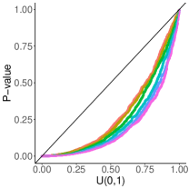
Refer to caption

(a)h=10,ฮด=1formulae-sequenceโ„Ž10๐›ฟ1h=10,\delta=1Refer to caption(b)h=10,ฮด=1formulae-sequenceโ„Ž10๐›ฟ1h=10,\delta=1Refer to caption(c)h=30,ฮด=1formulae-sequenceโ„Ž30๐›ฟ1h=30,\delta=1Refer to caption(d)h=10,ฮด=2formulae-sequenceโ„Ž10๐›ฟ2h=10,\delta=2

Figure 10: QQ plot of p๐‘p-values for L0subscript๐ฟ0L_{0} segmentation; hโ„Žh is the window size and ฮด๐›ฟ\delta the size of the change in the model from which we simulate. In (a), p๐‘p-values from our method are plotted against theoretical quantiles from Uโ€‹(0,1)๐‘ˆ01U(0,1) for N=1,2,5,10,20,50๐‘125102050N=1,2,5,10,20,50. (b), (c) and (d) show QQ plots of p๐‘p-values calculated using our method (with N=2,5,10,20,50๐‘25102050N=2,5,10,20,50) against p๐‘p-values from the method of Jewell etย al., (2022) (equivalent to N=1๐‘1N=1).
Refer to caption

h=10โ„Ž10h=10Refer to captionh=20โ„Ž20h=20Refer to captionh=30โ„Ž30h=30

Figure 11: Rejection rates of H0subscript๐ป0H_{0} for L0subscript๐ฟ0L_{0} segmentation. On each plot the three lines show the proportion of samples (of 1000 total) where the p๐‘p-value was below 0.050.050.05, resulting in H0subscript๐ป0H_{0} being rejected, for different values of N๐‘N. Each line corresponds to a different size of change ฮด๐›ฟ\delta: green corresponds to ฮด=3๐›ฟ3\delta=3, blue to ฮด=2๐›ฟ2\delta=2, and red to ฮด=1๐›ฟ1\delta=1.
Refer to caption

h=10โ„Ž10h=10Refer to captionh=20โ„Ž20h=20Refer to captionh=30โ„Ž30h=30

Figure 12: Rejection rates of H0subscript๐ป0H_{0} for different values of hโ„Žh, ฮด๐›ฟ\delta, and N๐‘N, when we simulate from a model with 4 changepoints, and apply wild binary segmentation with 4 changepoints. For each hโ„Žh, the process is run three times with changes of size ฮด=1,2,3๐›ฟ123\delta=1,2,3, which are shown on the plots as red, blue, and green lines respectively. Each line corresponds to a changepoint.

Figure 13 shows the results of applying L0subscript๐ฟ0L_{0} segmentation to the GC content data set we used in Section 5. The p๐‘p-values correspond to those in Table 3.

Refer to caption
Refer to caption
Refer to caption
Figure 13: Estimated changepoints in GC content data. L0subscript๐ฟ0L_{0} segmentation was used to estimate 38 changepoints, and we set h=10โ„Ž10h=10. Each vertical line corresponds to an estimated changepoint; changepoints found to be significant at significance level ฮฑ=0.05๐›ผ0.05\alpha=0.05 are shown in red, with others shown in grey. In the top panel, we used N=1๐‘1N=1 (equivalent to the method of Jewell etย al., (2022)) to calculate p๐‘p-values. The middle and bottom panels show results obtained using N=10๐‘10N=10 and N=20๐‘20N=20 respectively.

B.2 Correlation of p๐‘p-values

To investigate empirically whether p๐‘p-values at distinct locations (i.e. non-overlapping regions of interest) are uncorrelated, we simulated from a model with T=400๐‘‡400T=400 and three changepoints at ฯ„=100,200,300๐œ100200300\tau=100,200,300. Using binary segmentation, changepoints were detected at ฯ„^=92,200,297^๐œ92200297\hat{\tau}=92,200,297. We set h=10โ„Ž10h=10, so that the regions of interest around each ฯ„^^๐œ\hat{\tau} were non-overlapping. For each ฯ„^^๐œ\hat{\tau}, we sampled ฯ•italic-ฯ•\phi from its (conditional) distribution 1000 times. For each ฯ•(j)superscriptitalic-ฯ•๐‘—\phi^{(j)}, we calculated ๐‘ฟโ€ฒโ€‹(ฯ•(j))superscript๐‘ฟโ€ฒsuperscriptitalic-ฯ•๐‘—\boldsymbol{X}^{\prime}(\phi^{(j)}), applied binary segmentation, and calculated the p๐‘p-values. We then calculated pairwise correlations between p๐‘p-values, which are displayed in Table 4. We find that the correlations in all cases are very close to 00, so empirically the p๐‘p-values at different changepoints appear to be uncorrelated, and it seems reasonable to treat them as independent.

Table 4: Investigating independence of p๐‘p-values: in each case we sample different ฯ•italic-ฯ•\phi values at the changepoint of interest (keeping the rest of the data the same), re-apply the changepoint model, and calculate p๐‘p-values at each changepoint. We then calculate the pairwise correlations between p๐‘p-values.
Changepoint of interest ฯโ€‹(ฯ„^1,ฯ„^2)๐œŒsubscript^๐œ1subscript^๐œ2\rho(\hat{\tau}_{1},\hat{\tau}_{2}) ฯโ€‹(ฯ„^1,ฯ„^3)๐œŒsubscript^๐œ1subscript^๐œ3\rho(\hat{\tau}_{1},\hat{\tau}_{3}) ฯโ€‹(ฯ„^2,ฯ„^3)๐œŒsubscript^๐œ2subscript^๐œ3\rho(\hat{\tau}_{2},\hat{\tau}_{3})
ฯ„^1subscript^๐œ1\hat{\tau}_{1} 0.042 0.014 0.005
ฯ„^2subscript^๐œ2\hat{\tau}_{2} 0.017 0.001 0.007
ฯ„^3subscript^๐œ3\hat{\tau}_{3} 0.065 0.021 0.029

B.3 Robustness to Laplace noise

Figure 14 shows QQ-plots for post-selection p๐‘p-values for data simulated with i.i.d. Laplace noise. Under H0subscript๐ป0H_{0}, the p๐‘p-values are approximately uniform on [0,1]01[0,1].

Refer to caption

H0subscript๐ป0H_{0}, s=0.5๐‘ 0.5s=0.5Refer to captionH0subscript๐ป0H_{0}, s=1๐‘ 1s=1Refer to captionH1subscript๐ป1H_{1}, s=0.5๐‘ 0.5s=0.5

Figure 14: QQ plots of p๐‘p-values obtained when simulating from a Laplace distribution under H0subscript๐ป0H_{0} and H1subscript๐ป1H_{1}; s๐‘ s is the scale parameter.

Appendix C Additional Tables

We present here fuller versions of Tables 1 and 2, giving results for T=250,500,1000๐‘‡2505001000T=250,500,1000. Table 5 corresponds to Table 1 and Table 6 to Table 2. The different value of T๐‘‡T give similar results for the numbers of true and false positives detected.

Table 7 gives further results for binary segmentation for one of the scenarios in Table 6, in the case where T=1000๐‘‡1000T=1000 and K=4๐พ4K=4. Here we compare different choices of threshold for the binary segmentation algorithm, to investigate the effect this has on the number of true positives discovered and on the error rate. The threshold used for previous results was 3. Here we see that using a lower threshold increases the number of false positives (as would be expected, since we are more likely to detect false changepoints), but the FWER and FDR are still below 5%.

Table 5: Simulating from H0subscript๐ป0H_{0}, we applied binary segmentation and MOSUM and calculated how many times H0subscript๐ป0H_{0} was falsely rejected. The table reports the mean number of estimated changepoints with adjusted p๐‘p-value below 0.05 across 1000 iterations, and the proportion of runs in which there was at least one false discovery, for both the Holm-Bonferroni and Benjamini-Hochberg procedures.
Mean false positives Proportion with โ‰ฅ1absent1\geq 1 false positive
H-B B-H H-B B-H
BS, N=1๐‘1N=1 0.03 0.03 0.03 0.03
T=250๐‘‡250T=250 BS, N=10๐‘10N=10 0.04 0.04 0.03 0.03
MOSUM 0.01 0.01
BS, N=1๐‘1N=1 0.03 0.03 0.03 0.03
T=500๐‘‡500T=500 BS, N=10๐‘10N=10 0.03 0.03 0.03 0.03
MOSUM 0.01 0.01
BS, N=1๐‘1N=1 0.03 0.03 0.03 0.03
T=1000๐‘‡1000T=1000 BS, N=10๐‘10N=10 0.03 0.04 0.03 0.03
MOSUM 0.01 0.01
Table 6: Mean number of true positives and error rate when simulating ๐‘ฟ๐‘ฟ\boldsymbol{X} with T๐‘‡T data points and K๐พK equally spaced changepoints, with ฮผ๐œ‡\mu alternating between 111 and โˆ’11-1, using binary segmentation and MOSUM. The error rate given is the family-wise error rate for the Holm-Bonferroni method, and the false discovery rate for the Benjamini-Hochberg method and for MOSUM. This is calculated as Fโ€‹Dโ€‹R=false positivesfalse positivesย +ย true positives๐น๐ท๐‘…false positivesfalse positivesย ย true positivesFDR=\frac{\text{false positives}}{\text{false positives }+\text{ true positives}}.
Mean true positives Error rate (%)
H-B B-H H-B B-H
BS, N=1๐‘1N=1 0.78 0.78 0.30 0.34
T=250,K=1formulae-sequence๐‘‡250๐พ1T=250,K=1 BS, N=10๐‘10N=10 0.94 0.50 0.27 0.34
MOSUM 0.74 1.08
BS, N=1๐‘1N=1 2.67 2.79 0.30 0.16
T=250,K=4formulae-sequence๐‘‡250๐พ4T=250,K=4 BS, N=10๐‘10N=10 3.45 3.55 0.70 0.24
MOSUM 2.83 0.18
BS, N=1๐‘1N=1 5.07 5.92 0.70 0.17
T=250,K=9formulae-sequence๐‘‡250๐พ9T=250,K=9 BS, N=10๐‘10N=10 7.24 7.74 0.50 0.12
MOSUM 6.43 0.03
BS, N=1๐‘1N=1 0.79 0.79 1.10 0.99
T=500,K=1formulae-sequence๐‘‡500๐พ1T=500,K=1 BS, N=10๐‘10N=10 0.95 0.95 1.60 0.93
MOSUM 0.63 1.26
BS, N=1๐‘1N=1 2.75 2.89 0.40 0.29
T=500,K=4formulae-sequence๐‘‡500๐พ4T=500,K=4 BS, N=10๐‘10N=10 3.46 3.53 1.00 0.35
MOSUM 2.59 0.27
BS, N=1๐‘1N=1 5.54 6.36 1.10 0.31
T=500,K=9formulae-sequence๐‘‡500๐พ9T=500,K=9 BS, N=10๐‘10N=10 7.38 7.87 1.30 0.33
MOSUM 5.89 0.07
BS, N=1๐‘1N=1 0.79 0.79 0.60 0.53
T=1000,K=1formulae-sequence๐‘‡1000๐พ1T=1000,K=1 BS, N=10๐‘10N=10 0.94 0.94 0.50 0.29
MOSUM 0.58 1.20
BS, N=1๐‘1N=1 2.78 2.91 0.90 0.42
T=1000,K=4formulae-sequence๐‘‡1000๐พ4T=1000,K=4 BS, N=10๐‘10N=10 3.42 3.51 1.50 0.46
MOSUM 2.32 0.22
BS, N=1๐‘1N=1 5.56 6.38 1.50 0.42
T=1000,K=9formulae-sequence๐‘‡1000๐พ9T=1000,K=9 BS, N=10๐‘10N=10 7.23 7.80 2.10 0.51
MOSUM 5.30 0.09
Table 7: Mean number of true positives and error rate when simulating from a model with T=1000๐‘‡1000T=1000 and K=4๐พ4K=4 equally spaced changepoints, with ฮผ๐œ‡\mu alternating between 111 and โˆ’11-1, using binary segmentation. The error rate given is the family-wise error rate for the Holm-Bonferroni method, and the false discovery rate for the Benjamini-Hochberg method. This is calculated as Fโ€‹Dโ€‹R=false positivesfalse positivesย +ย true positives๐น๐ท๐‘…false positivesfalse positivesย ย true positivesFDR=\frac{\text{false positives}}{\text{false positives }+\text{ true positives}}.
Mean true positives Error rate (%)
Threshold N๐‘N H-B B-H H-B B-H
2 N=1๐‘1N=1 2.70 3.02 3.10 2.89
3 N=1๐‘1N=1 2.78 2.91 0.90 0.42
4 N=1๐‘1N=1 2.49 2.63 0.30 0.11
2 N=10๐‘10N=10 3.33 3.60 3.80 2.83
3 N=10๐‘10N=10 3.42 3.51 1.50 0.46
4 N=10๐‘10N=10 3.51 3.57 0.30 0.08