Linear Computation Coding:
Exponential Search and Reduced-State Algorithms

Abstract

Linear computation coding is concerned with the compression of multidimensional linear functions, i.e. with reducing the computational effort of multiplying an arbitrary vector to an arbitrary, but known, constant matrix. This paper advances over the state-of-the art, that is based on a discrete matching pursuit (DMP) algorithm, by a step-wise optimal search. Offering significant performance gains over DMP, it is however computationally infeasible for large matrices and high accuracy. Therefore, a reduced-state algorithm is introduced that offers performance superior to DMP, while still being computationally feasible even for large matrices. Depending on the matrix size, the performance gain over DMP is on the order of at least $10\text{\,}\mathrm{\char 37\relax}$.

1 Introduction

Multiplying a vector by a constant matrix is an ubiquitous task performed in various technical and scientific applications. The main body of earlier work is focused on speeding up the calculation of matrix-vector multiplications in a structure-oriented fashion. A well-known example is the fast implementation of the discrete fourier transform (DFT). Here, the structure of the DFT matrix is exploited to eliminate redundant computations and reduce the number of required operations as compared to a naive implementation. For arbitrary constant matrices, redundancies within the finite-precision representation of the matrix entries can be exploited as well, a method that is typically known as common subexpression sharing/elimination. Earlier work in this respect has either targeted special cases of constant multiplication [1, 2] or has proposed schemes with high computational complexity, such that their implementation in practice is difficult for medium to large size matrices [3, 4].

Recently, linear computation coding (LCC) has been proposed in [5, 6, 7]. This framework develops an information-theoretic scheme for the efficient calculation of matrix-vector products that is especially well-suited for the implementation on reconfigurable hardware, such as field programmable gate arrays [8]. Similar to rate-distortion theory, LCC is concerned with the tradeoff between distortion and compression. However, instead of compressing data, LCC deals with the lossy compression of multidimensional linear functions under a given fidelity constraint. An instance can be found in [7], where an optimal decomposition scheme is first defined in terms of classical metrics for computation and distortion. A greedy approach is then developed to approximate the proposed scheme sub-optimally with tractable complexity.

Contributions In this paper, we develop a new LCC scheme. Similar to earlier approaches discussed in [7], the optimal decomposition deals with an exponentially complex problem. We first address this problem via an exhaustive search procedure with a careful optimization. This enables us to evaluate the performance of the optimal scheme for reasonable matrix sizes. We then present a computationally tractable scheme by proposing a reduced-state algorithm for the underlying search problem. Our investigations show that the proposed algorithm can achieve a computation-distortion tradeoff close to the exponentially-complex optimal scheme while drastically reducing the decomposition complexity.

Notation Vectors are denoted as lower-case boldface letters $\textstyle x$ and matrices as upper-case boldface letters $\textstyle X$. The Euclidean and the Frobenius norm are denoted by $\|\cdot\|_{2}$ and $\|\cdot\|_{\mathrm{F}}$, respectively. The symbol ${\mathchoice{\mbox{\boldmath$\displaystyle 0$}}{\mbox{\boldmath$\textstyle 0$}}{\mbox{\boldmath$\scriptstyle 0$}}{\mbox{\boldmath$\scriptscriptstyle 0$}}}_{N\times K}$ denotes an $N\times K$ matrix with all zero elements, ${\mathchoice{\mbox{\boldmath$\displaystyle I$}}{\mbox{\boldmath$\textstyle I$}}{\mbox{\boldmath$\scriptstyle I$}}{\mbox{\boldmath$\scriptscriptstyle I$}}}_{N\times K}$ denotes the augmented identity matrix of dimension $N\times K$ and ${\mathchoice{\mbox{\boldmath$\displaystyle 1$}}{\mbox{\boldmath$\textstyle 1$}}{\mbox{\boldmath$\scriptstyle 1$}}{\mbox{\boldmath$\scriptscriptstyle 1$}}}_{j,K}$ denotes the $j$-th row unit vector in $K$ dimensions.

2 Problem Formulation

We consider the problem of matrix-vector multiplication, i.e the calculation

$${\mathchoice{\mbox{\boldmath$\displaystyle y$}}{\mbox{\boldmath$\textstyle y$}}{\mbox{\boldmath$\scriptstyle y$}}{\mbox{\boldmath$\scriptscriptstyle y$}}}={\mathchoice{\mbox{\boldmath$\displaystyle A$}}{\mbox{\boldmath$\textstyle A$}}{\mbox{\boldmath$\scriptstyle A$}}{\mbox{\boldmath$\scriptscriptstyle A$}}}{\mathchoice{\mbox{\boldmath$\displaystyle x$}}{\mbox{\boldmath$\textstyle x$}}{\mbox{\boldmath$\scriptstyle x$}}{\mbox{\boldmath$\scriptscriptstyle x$}}}$$ (1)

for an arbitrary input vector ${\mathchoice{\mbox{\boldmath$\displaystyle x$}}{\mbox{\boldmath$\textstyle x$}}{\mbox{\boldmath$\scriptstyle x$}}{\mbox{\boldmath$\scriptscriptstyle x$}}}\in\mathbb{R}^{K\times 1}$ and a constant matrix ${\mathchoice{\mbox{\boldmath$\displaystyle A$}}{\mbox{\boldmath$\textstyle A$}}{\mbox{\boldmath$\scriptstyle A$}}{\mbox{\boldmath$\scriptscriptstyle A$}}}\in\mathbb{R}^{N\times K}$. Commonly, matrices are approximated by quantizing their entries independently. By using the canonically signed digit (CSD) binary representation the quantization error can be decreased on average by a factor of $\sqrt{28}$ per CSD [9]. This still leaves room for improvement. LCC instead suggests to approximate $\textstyle A$ by a product of matrices, i.e. finding $\textstyle W$ and $\textstyle C$ such that

$${\mathchoice{\mbox{\boldmath$\displaystyle A$}}{\mbox{\boldmath$\textstyle A$}}{\mbox{\boldmath$\scriptstyle A$}}{\mbox{\boldmath$\scriptscriptstyle A$}}}\approx{\mathchoice{\mbox{\boldmath$\displaystyle W$}}{\mbox{\boldmath$\textstyle W$}}{\mbox{\boldmath$\scriptstyle W$}}{\mbox{\boldmath$\scriptscriptstyle W$}}}{\mathchoice{\mbox{\boldmath$\displaystyle C$}}{\mbox{\boldmath$\textstyle C$}}{\mbox{\boldmath$\scriptstyle C$}}{\mbox{\boldmath$\scriptscriptstyle C$}}}.$$ (2)

The matrix ${\mathchoice{\mbox{\boldmath$\displaystyle C$}}{\mbox{\boldmath$\textstyle C$}}{\mbox{\boldmath$\scriptstyle C$}}{\mbox{\boldmath$\scriptscriptstyle C$}}}\in\mathcal{A}^{N\times K}$ is termed the codebook matrix and ${\mathchoice{\mbox{\boldmath$\displaystyle W$}}{\mbox{\boldmath$\textstyle W$}}{\mbox{\boldmath$\scriptstyle W$}}{\mbox{\boldmath$\scriptscriptstyle W$}}}\in\mathcal{A}^{N\times N}$ is termed the wiring matrix in the sequel. The entries of the wiring matrix are restricted to the set of zero and signed powers of two ($\mathcal{A}\subseteq\{0,\pm 2^{\mathbb{Z}}\}$).

Obtaining the wiring and codebook matrix jointly is typically NP-hard and infeasible. To overcome this computational intractability, [7] proposes a scheme where the $n$-th row of the wiring matrix is determined by solving the following sparse recovery problem for some design parameter $S<N$ controlling the cost between distortion and computation effort [10]

$${\mathchoice{\mbox{\boldmath$\displaystyle w$}}{\mbox{\boldmath$\textstyle w$}}{\mbox{\boldmath$\scriptstyle w$}}{\mbox{\boldmath$\scriptscriptstyle w$}}}_{n}=\underset{{\mathchoice{\mbox{\boldmath$\displaystyle\omega$}}{\mbox{\boldmath$\textstyle\omega$}}{\mbox{\boldmath$\scriptstyle\omega$}}{\mbox{\boldmath$\scriptscriptstyle\omega$}}}\in\{{\mathchoice{\mbox{\boldmath$\displaystyle\omega$}}{\mbox{\boldmath$\textstyle\omega$}}{\mbox{\boldmath$\scriptstyle\omega$}}{\mbox{\boldmath$\scriptscriptstyle\omega$}}}=\sum_{s=1}^{S}i_{s}{\mathchoice{\mbox{\boldmath$\displaystyle 1$}}{\mbox{\boldmath$\textstyle 1$}}{\mbox{\boldmath$\scriptstyle 1$}}{\mbox{\boldmath$\scriptscriptstyle 1$}}}_{j_{s},N}:\;i_{s}\in\mathcal{A},\,j_{s}\in\{1,...,N\}\;\forall s\}}{\mathop{\mathrm{argmin}}}\|{\mathchoice{\mbox{\boldmath$\displaystyle a$}}{\mbox{\boldmath$\textstyle a$}}{\mbox{\boldmath$\scriptstyle a$}}{\mbox{\boldmath$\scriptscriptstyle a$}}}_{n}-{\mathchoice{\mbox{\boldmath$\displaystyle\omega$}}{\mbox{\boldmath$\textstyle\omega$}}{\mbox{\boldmath$\scriptstyle\omega$}}{\mbox{\boldmath$\scriptscriptstyle\omega$}}}{\mathchoice{\mbox{\boldmath$\displaystyle C$}}{\mbox{\boldmath$\textstyle C$}}{\mbox{\boldmath$\scriptstyle C$}}{\mbox{\boldmath$\scriptscriptstyle C$}}}\|_{2}\quad\forall n.$$ (3)

The new scheme is still NP-hard, but not in $N$, anymore, but in $S$. Thus, small values of $S$ are required, in practice.

In order to have a high accuracy despite small values of $S$, the factorization procedure can be applied multiple times. Then the product ${\mathchoice{\mbox{\boldmath$\displaystyle C$}}{\mbox{\boldmath$\textstyle C$}}{\mbox{\boldmath$\scriptstyle C$}}{\mbox{\boldmath$\scriptscriptstyle C$}}}_{i}={\mathchoice{\mbox{\boldmath$\displaystyle W$}}{\mbox{\boldmath$\textstyle W$}}{\mbox{\boldmath$\scriptstyle W$}}{\mbox{\boldmath$\scriptscriptstyle W$}}}_{i}{\mathchoice{\mbox{\boldmath$\displaystyle C$}}{\mbox{\boldmath$\textstyle C$}}{\mbox{\boldmath$\scriptstyle C$}}{\mbox{\boldmath$\scriptscriptstyle C$}}}_{i-1}$ of the previous wiring step acts as the new codebook for obtaining the following matrix factor ${\mathchoice{\mbox{\boldmath$\displaystyle W$}}{\mbox{\boldmath$\textstyle W$}}{\mbox{\boldmath$\scriptstyle W$}}{\mbox{\boldmath$\scriptscriptstyle W$}}}_{i}$ of the current wiring step. Hence, by setting ${\mathchoice{\mbox{\boldmath$\displaystyle C$}}{\mbox{\boldmath$\textstyle C$}}{\mbox{\boldmath$\scriptstyle C$}}{\mbox{\boldmath$\scriptscriptstyle C$}}}_{0}={\mathchoice{\mbox{\boldmath$\displaystyle I$}}{\mbox{\boldmath$\textstyle I$}}{\mbox{\boldmath$\scriptstyle I$}}{\mbox{\boldmath$\scriptscriptstyle I$}}}_{N\times K}$, we obtain the approximated matrix $\textstyle P$ after $I$ wiring steps:

$${\mathchoice{\mbox{\boldmath$\displaystyle A$}}{\mbox{\boldmath$\textstyle A$}}{\mbox{\boldmath$\scriptstyle A$}}{\mbox{\boldmath$\scriptscriptstyle A$}}}\approx{\mathchoice{\mbox{\boldmath$\displaystyle P$}}{\mbox{\boldmath$\textstyle P$}}{\mbox{\boldmath$\scriptstyle P$}}{\mbox{\boldmath$\scriptscriptstyle P$}}}=\left(\prod_{i=1}^{I}{\mathchoice{\mbox{\boldmath$\displaystyle W$}}{\mbox{\boldmath$\textstyle W$}}{\mbox{\boldmath$\scriptstyle W$}}{\mbox{\boldmath$\scriptscriptstyle W$}}}_{i}\right){\mathchoice{\mbox{\boldmath$\displaystyle C$}}{\mbox{\boldmath$\textstyle C$}}{\mbox{\boldmath$\scriptstyle C$}}{\mbox{\boldmath$\scriptscriptstyle C$}}}_{0}.$$ (4)

To quantify the accuracy of a given approximation $\textstyle P$ we use the signal-to-quantization-noise-ratio (SQNR)

$$\mathrm{SQNR}({\mathchoice{\mbox{\boldmath$\displaystyle A$}}{\mbox{\boldmath$\textstyle A$}}{\mbox{\boldmath$\scriptstyle A$}}{\mbox{\boldmath$\scriptscriptstyle A$}}},{\mathchoice{\mbox{\boldmath$\displaystyle P$}}{\mbox{\boldmath$\textstyle P$}}{\mbox{\boldmath$\scriptstyle P$}}{\mbox{\boldmath$\scriptscriptstyle P$}}})=\frac{\|{\mathchoice{\mbox{\boldmath$\displaystyle A$}}{\mbox{\boldmath$\textstyle A$}}{\mbox{\boldmath$\scriptstyle A$}}{\mbox{\boldmath$\scriptscriptstyle A$}}}\|_{\mathrm{F}}^{2}}{\|{\mathchoice{\mbox{\boldmath$\displaystyle A$}}{\mbox{\boldmath$\textstyle A$}}{\mbox{\boldmath$\scriptstyle A$}}{\mbox{\boldmath$\scriptscriptstyle A$}}}-{\mathchoice{\mbox{\boldmath$\displaystyle P$}}{\mbox{\boldmath$\textstyle P$}}{\mbox{\boldmath$\scriptstyle P$}}{\mbox{\boldmath$\scriptscriptstyle P$}}}\|_{\mathrm{F}}^{2}}.$$ (5)

Computational Cost In a binary number representation the multiplication by a signed power of two corresponds only to a bitshift. On reconfigurable hardware, this shift can be realized simply by appropriate wiring without the need for dedicated processing elements such as adders [8]. The parameter $S$ in (3) determines the number of vectors from the codebook to be used in forming the linear combination to approximate a row ${\mathchoice{\mbox{\boldmath$\displaystyle a$}}{\mbox{\boldmath$\textstyle a$}}{\mbox{\boldmath$\scriptstyle a$}}{\mbox{\boldmath$\scriptscriptstyle a$}}}_{n}$ of $\textstyle A$. It therefore directly controls the computational cost, as in computing the linear combination, exactly $S-1$ additions are required. No multiplications, except by signed powers of two, are necessary due to the specific structure of the wiring matrix. Therefore, the separate product of the decomposed matrices with the input vector ${\mathchoice{\mbox{\boldmath$\displaystyle y$}}{\mbox{\boldmath$\textstyle y$}}{\mbox{\boldmath$\scriptstyle y$}}{\mbox{\boldmath$\scriptscriptstyle y$}}}\approx{\mathchoice{\mbox{\boldmath$\displaystyle W$}}{\mbox{\boldmath$\textstyle W$}}{\mbox{\boldmath$\scriptstyle W$}}{\mbox{\boldmath$\scriptscriptstyle W$}}}({\mathchoice{\mbox{\boldmath$\displaystyle C$}}{\mbox{\boldmath$\textstyle C$}}{\mbox{\boldmath$\scriptstyle C$}}{\mbox{\boldmath$\scriptscriptstyle C$}}}{\mathchoice{\mbox{\boldmath$\displaystyle x$}}{\mbox{\boldmath$\textstyle x$}}{\mbox{\boldmath$\scriptstyle x$}}{\mbox{\boldmath$\scriptscriptstyle x$}}})$ is much simpler to compute than calculating the product in (1) straightforwardly.

The total computational cost $C_{\mathrm{add}}$ of a decomposition in (4) is given by the number of additions (or subtractions) required to form the linear combinations

$$C_{\mathrm{add}}=IN(S-1).$$ (6)

3 Algorithms

In this section we will briefly look at the state of the art for solving the optimization problem in (3) to obtain the wiring matrices and then introduce two improved novel algorithms.

State-of-the-Art: Discrete Matching Pursuit The DMP follows the matching pursuit approach to successively determine the wiring coefficients. The algorithm can be summarized in the following key steps; for details see [6].

1. Start with iteration $s\leftarrow 0$. Initialize ${\mathchoice{\mbox{\boldmath$\displaystyle\omega$}}{\mbox{\boldmath$\textstyle\omega$}}{\mbox{\boldmath$\scriptstyle\omega$}}{\mbox{\boldmath$\scriptscriptstyle\omega$}}}\leftarrow{\mathchoice{\mbox{\boldmath$\displaystyle 0$}}{\mbox{\boldmath$\textstyle 0$}}{\mbox{\boldmath$\scriptstyle 0$}}{\mbox{\boldmath$\scriptscriptstyle 0$}}}_{1\times N}$

2. Update $\textstyle\omega$ in at most a single component, such that $\|{\mathchoice{\mbox{\boldmath$\displaystyle a_{n}$}}{\mbox{\boldmath$\textstyle a_{n}$}}{\mbox{\boldmath$\scriptstyle a_{n}$}}{\mbox{\boldmath$\scriptscriptstyle a_{n}$}}}-{\mathchoice{\mbox{\boldmath$\displaystyle\omega$}}{\mbox{\boldmath$\textstyle\omega$}}{\mbox{\boldmath$\scriptstyle\omega$}}{\mbox{\boldmath$\scriptscriptstyle\omega$}}}{\mathchoice{\mbox{\boldmath$\displaystyle C$}}{\mbox{\boldmath$\textstyle C$}}{\mbox{\boldmath$\scriptstyle C$}}{\mbox{\boldmath$\scriptscriptstyle C$}}}\|_{2}$ is minimized.

3. Increment $s$.

4. If $s\leq S$, go to step 2, otherwise the procedure terminates.

It is straightforward to show that the time complexity of the DMP algorithm for computing a single matrix factor scales with $\mathcal{O}(N^{3}S)$.

Exponential Search Algorithm The row-wise optimization problem in (3) is NP-hard. However, for small $S$, reasonable matrix sizes and some careful optimization it can be solved in a tractable timeframe. We limit the set of scaling factors to a finite set of signed powers of two ($\mathcal{A}_{\mathrm{exp}}\subset\{0,\pm 2^{\mathbb{Z}}\}$), as an exhaustive search over the whole set is infeasible. As the search procedure has to be performed for each row of the target matrix individually, the time complexity for the computation of each wiring step is given by $\mathcal{O}(N^{S}|\mathcal{A_{\mathrm{exp}}}|^{S})$.

Generally, which and how many coefficients are included in the subset $\mathcal{A}_{\mathrm{exp}}$ is a design parameter and needs to be adapted to each specific decomposition. It depends primarily on two factors. First, the current wiring step plays a crucial role. For each additional wiring layer, the error between each row of the target matrix and the approximated matrix decreases. Hence, for any subsequent wiring step, smaller coefficients are needed to scale the rows of the newly found codebook matrix to appropriately approximate the residual error. This also means that for high desired accuracy the coefficient set needs to be chosen large, i.e. to include also many small coefficients, to accurately approximate the error. Furthermore, relative variations in the length of the row vectors of the target matrix require a larger coefficient set to compensate for differences. Still, to keep the decomposition computationally feasible, the number of elements in $\mathcal{A}_{\mathrm{exp}}$ needs to be chosen as small as possible, as the computational complexity scales exponentially in $S$ with the product of the size of the coefficient set $|\mathcal{A}_{\mathrm{exp}}|$ and $N$ as base.

A promising approach for further research is to adapt the coefficient set for each wiring step dynamically based on the current fidelity of the approximation. The coefficient set may then be determined from the probability distribution of the likely entries of the wiring matrix.

Reduced-State Algorithm The runtime of the exponential algorithm for a matrix with $N=64$ rows is on the order of an hour, for larger matrices the runtime scales up accordingly and can become infeasible. Hence, for some applications the computational burden of the exponential algorithm might consequently not be feasible. A reasonable compromise between complexity and performance is desirable.

Unlike in DMP, we do not immediately update the components of the wiring vector for the reduced-state algorithm. Instead, we keep updating in each iteration a list of the $M$ best vectors, which minimize (3) and select at the termination of the algorithm the vector with minimum error from the list. Specifically, we apply the following successive, greedy procedure for the optimization problem in (3):

1. Start with $s\leftarrow 0$. Initialize the set $\Omega$ with $M$ all-zero vectors.

2. For each ${\mathchoice{\mbox{\boldmath$\displaystyle\omega$}}{\mbox{\boldmath$\textstyle\omega$}}{\mbox{\boldmath$\scriptstyle\omega$}}{\mbox{\boldmath$\scriptscriptstyle\omega$}}}\in\Omega$ find the set $\Omega_{m}$ of $M$ mutually distinct vectors ${\mathchoice{\mbox{\boldmath$\displaystyle\omega$}}{\mbox{\boldmath$\textstyle\omega$}}{\mbox{\boldmath$\scriptstyle\omega$}}{\mbox{\boldmath$\scriptscriptstyle\omega$}}}_{\tilde{m}}$ with $\tilde{m}\in\{1,...,M\}$ that minimize $\|{\mathchoice{\mbox{\boldmath$\displaystyle a$}}{\mbox{\boldmath$\textstyle a$}}{\mbox{\boldmath$\scriptstyle a$}}{\mbox{\boldmath$\scriptscriptstyle a$}}}_{n}-{\mathchoice{\mbox{\boldmath$\displaystyle\omega$}}{\mbox{\boldmath$\textstyle\omega$}}{\mbox{\boldmath$\scriptstyle\omega$}}{\mbox{\boldmath$\scriptscriptstyle\omega$}}}_{\tilde{m}}{\mathchoice{\mbox{\boldmath$\displaystyle C$}}{\mbox{\boldmath$\textstyle C$}}{\mbox{\boldmath$\scriptstyle C$}}{\mbox{\boldmath$\scriptscriptstyle C$}}}\|_{2}$ and differ from $\textstyle\omega$ in at most a single component.

3. Update the set $\Omega$ by selecting from $\bigcup_{m=1}^{M}\Omega_{m}$ the $M$ distinct vectors $\textstyle\omega$ with minimum $\|{\mathchoice{\mbox{\boldmath$\displaystyle a$}}{\mbox{\boldmath$\textstyle a$}}{\mbox{\boldmath$\scriptstyle a$}}{\mbox{\boldmath$\scriptscriptstyle a$}}}_{n}-{\mathchoice{\mbox{\boldmath$\displaystyle\omega$}}{\mbox{\boldmath$\textstyle\omega$}}{\mbox{\boldmath$\scriptstyle\omega$}}{\mbox{\boldmath$\scriptscriptstyle\omega$}}}{\mathchoice{\mbox{\boldmath$\displaystyle C$}}{\mbox{\boldmath$\textstyle C$}}{\mbox{\boldmath$\scriptstyle C$}}{\mbox{\boldmath$\scriptscriptstyle C$}}}\|_{2}$

4. Increment $s$.

5. If $s\leq S$, go to step 2, else, continue

6. Return $\underset{{\mathchoice{\mbox{\boldmath$\displaystyle\omega$}}{\mbox{\boldmath$\textstyle\omega$}}{\mbox{\boldmath$\scriptstyle\omega$}}{\mbox{\boldmath$\scriptscriptstyle\omega$}}}\in\Omega}{\mathop{\mathrm{argmin}}}\|{\mathchoice{\mbox{\boldmath$\displaystyle a$}}{\mbox{\boldmath$\textstyle a$}}{\mbox{\boldmath$\scriptstyle a$}}{\mbox{\boldmath$\scriptscriptstyle a$}}}_{n}-{\mathchoice{\mbox{\boldmath$\displaystyle\omega$}}{\mbox{\boldmath$\textstyle\omega$}}{\mbox{\boldmath$\scriptstyle\omega$}}{\mbox{\boldmath$\scriptscriptstyle\omega$}}}{\mathchoice{\mbox{\boldmath$\displaystyle C$}}{\mbox{\boldmath$\textstyle C$}}{\mbox{\boldmath$\scriptstyle C$}}{\mbox{\boldmath$\scriptscriptstyle C$}}}\|_{2}$

By tuning $M$, we are able to adjust the space of possible combinations that the algorithm explores. For each wiring step, we have to evaluate $\mathcal{O}(SN^{3}M^{2})$ combinations. Compared to DMP the complexity is increased by a factor of $M^{2}$. Note that for $M=1$ the algorithm reduces to the DMP.

4 Numerical Evaluation

In this section, we compare the performance of the proposed algorithms to the baseline DMP [7]. We decompose matrices whose entries are drawn i.i.d. from a Gaussian distribution with zero mean and unit variance. Similar to DMP, the performance of the improved versions of the algorithm hardly depends on the distribution of the matrix elements. The algorithms are invariant to scaling of the variance, however it is crucial that for the exponential search algorithm the coefficient set $\mathcal{A}_{\mathrm{exp}}$ is scaled appropriately as well, as to not compromise performance. Throughout the simulations, we select the coefficient set for the exponential search algorithm to $\mathcal{A}_{\mathrm{exp}}=\{\pm 2^{-40},..,\pm 2^{3}\}$.

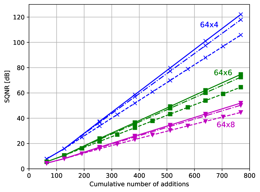
As a first experiment, we compare all three algorithms for fixed matrix sizes in Figure 1. We choose matrices with $N=64$ rows and vary the number of columns $K$ from four to eight. Hence, we can compare the performance for different aspect ratios of the matrices. To quantify performance, we plot the tradeoff between distortion and computational cost. The latter being measured by the number of cumulative additions $C_{\mathrm{add}}$ required for a given wiring step.

As Figure 1 shows, for all three matrix sizes there is a performance gain by both proposed algorithms against DMP. Further, for memory size $M=10$, the reduced state algorithm performs only slightly worse than exhaustive search.

Figure 1: Performance comparison for matrices with 64 rows and different aspect ratios. Matrices of dimension $64\times 4$ are indicated by crosses, $64\times 6$ is indicated by squares and $64\times 8$ is indicated by triangles. The solid lines refer to the exponential search algorithm ($S=3$), the dashed lines to the DMP [7] ($S=2$) and the dashed-dotted lines to the reduced state algorithm with memory size $M=10$ and $S=3$. Results are averaged over $10^{4}$ matrix entries for the exponential search algorithm and over $10^{5}$ matrix entries for the other algorithms.

For the first two wiring steps, the performance of all three algorithms is equal for a given matrix size. This is due to the fact that for the first two steps we use DMP with $S=2$ for an initial refinement of the codebook. Applying any of the algorithms with $S\geq 3$ directly to the initial codebook ${\mathchoice{\mbox{\boldmath$\displaystyle C$}}{\mbox{\boldmath$\textstyle C$}}{\mbox{\boldmath$\scriptstyle C$}}{\mbox{\boldmath$\scriptscriptstyle C$}}}_{0}={\mathchoice{\mbox{\boldmath$\displaystyle I$}}{\mbox{\boldmath$\textstyle I$}}{\mbox{\boldmath$\scriptstyle I$}}{\mbox{\boldmath$\scriptscriptstyle I$}}}_{N\times K}$ would lead to degraded performance for the first few wiring steps. Instead it is beneficial to set $S=2$ to allow for more frequent updates of the codebook in the beginning. From empirical investigations it seems that two wiring iterations with $S=2$ are most beneficial for the overall performance.

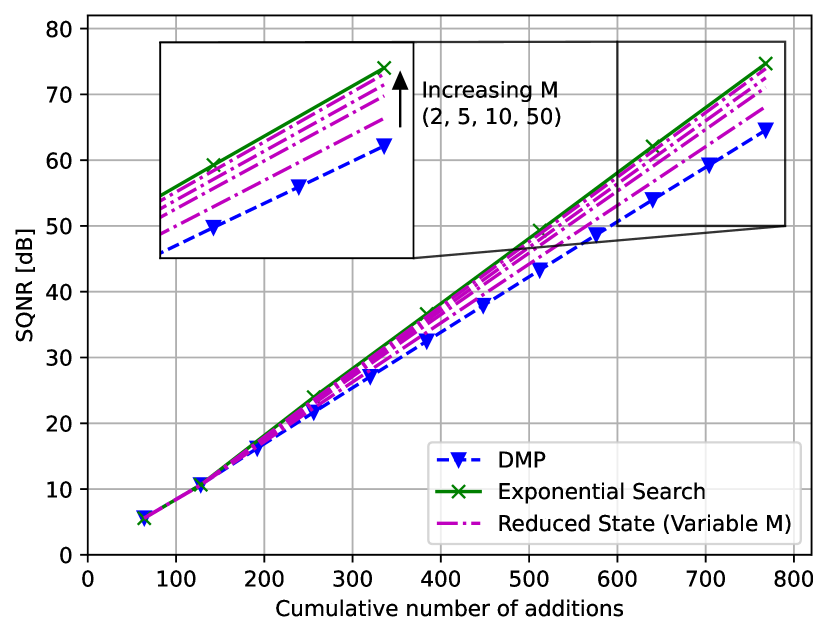
Figure 2: Performance comparison for different memory sizes $M$ of the reduced state algorithm of a $64\times 6$ matrix. The solid line refers to the exponential search algorithm ($S=3$), the dashed line to the DMP [7] ($S=2$) and the dashed-dotted lines to the reduced state algorithm with 4 different memory sizes and $S=3$. Results are averaged over $10^{4}$ matrix entries for the exponential search algorithm and over $10^{5}$ matrix entries for the other algorithms.

As the next experiment, we compare the performance of the reduced state algorithm for different choices of the memory parameter $M$ for given matrix size of $64\times 6$ in Figure 2. From the figure we observe that even for small $M$ the reduced state algorithm offers a noticeable performance gain over DMP. As $M$ grows, the reduced state algorithm approaches the performance of the exponential search. The large advantage of the reduced state algorithm is that the computation time is reduced drastically. For $M=1$ the reduced state algorithm reduces to DMP and both lines coincide for any given matrix size.

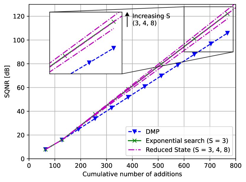
Figure 3: Performance comparison for different choices of the parameter $S$ of a matrix with dimension $64\times 4$. The solid line refers to the exponential search algorithm ($S=3$), the dashed line to the DMP [7] ($S=2$) and the dashed-dotted lines to the reduced state algorithm with different choices of the parameter $S$ and $M=10$. Results are averaged over $10^{4}$ matrix entries for the exponential search algorithm and over $10^{5}$ matrix entries for the other algorithms.

Table 1 lists the relative performance gains over DMP for various matrix sizes and configurations of the algorithms.

Table 1: Relative average gain in terms of SQNR of the novel algorithms over the baseline DMP algorithm with $S=2$ (For at least $8\text{\,}\mathrm{b}\mathrm{i}\mathrm{t}$ signed integer accuracy ($10\log(\textrm{SQNR})\geq$47\text{\,}\mathrm{dB}$$)). Results are averaged over $10^{4}$ matrix entries for the exponential search algorithm and over $10^{5}$ matrix entries for the other algorithms.

	Exponential	Reduced State
	search	$S=3$		$S=4$		$S=8$
Matrix size	$S=3$	$M=5$	$M=10$	$M=5$	$M=10$	$M=5$	$M=10$
$16\times 2$	$17.8\text{\,}\mathrm{\char 37\relax}$	$10.4\text{\,}\mathrm{\char 37\relax}$	$13.4\text{\,}\mathrm{\char 37\relax}$	$14.1\text{\,}\mathrm{\char 37\relax}$	$17.8\text{\,}\mathrm{\char 37\relax}$	$16.7\text{\,}\mathrm{\char 37\relax}$	$21.9\text{\,}\mathrm{\char 37\relax}$
$16\times 4$	$34.5\text{\,}\mathrm{\char 37\relax}$	$16.0\text{\,}\mathrm{\char 37\relax}$	$24.5\text{\,}\mathrm{\char 37\relax}$	$25.8\text{\,}\mathrm{\char 37\relax}$	$32.7\text{\,}\mathrm{\char 37\relax}$	$25.4\text{\,}\mathrm{\char 37\relax}$	$34.4\text{\,}\mathrm{\char 37\relax}$
$32\times 4$	$15.7\text{\,}\mathrm{\char 37\relax}$	$10.5\text{\,}\mathrm{\char 37\relax}$	$12.9\text{\,}\mathrm{\char 37\relax}$	$14.0\text{\,}\mathrm{\char 37\relax}$	$17.2\text{\,}\mathrm{\char 37\relax}$	$18.4\text{\,}\mathrm{\char 37\relax}$	$22.3\text{\,}\mathrm{\char 37\relax}$
$32\times 6$	$25.3\text{\,}\mathrm{\char 37\relax}$	$15.5\text{\,}\mathrm{\char 37\relax}$	$19.0\text{\,}\mathrm{\char 37\relax}$	$19.7\text{\,}\mathrm{\char 37\relax}$	$24.5\text{\,}\mathrm{\char 37\relax}$	$19.4\text{\,}\mathrm{\char 37\relax}$	$26.0\text{\,}\mathrm{\char 37\relax}$
$64\times 4$	$12.9\text{\,}\mathrm{\char 37\relax}$	$7.5\text{\,}\mathrm{\char 37\relax}$	$9.8\text{\,}\mathrm{\char 37\relax}$	$11.0\text{\,}\mathrm{\char 37\relax}$	$13.8\text{\,}\mathrm{\char 37\relax}$	$13.5\text{\,}\mathrm{\char 37\relax}$	$16.8\text{\,}\mathrm{\char 37\relax}$
$64\times 6$	$14.9\text{\,}\mathrm{\char 37\relax}$	$9.6\text{\,}\mathrm{\char 37\relax}$	$11.4\text{\,}\mathrm{\char 37\relax}$	$13.6\text{\,}\mathrm{\char 37\relax}$	$16.5\text{\,}\mathrm{\char 37\relax}$	$15.6\text{\,}\mathrm{\char 37\relax}$	$19.0\text{\,}\mathrm{\char 37\relax}$

Practical Considerations for the Choice of $S$ Figure 3 shows the performance of the reduced state algorithm for varying $S$. Due to the exponentially growing complexity in $S$, the exponential algorithm is not feasible for $S>3$, except for very small matrices. We can observe, that by choosing $S=4$ for the reduced state algorithm, we approximately achieve the same distortion-cost tradeoff as for the exponential algorithm with $S=3$. For choosing $S$ even larger the gains increase likewise.

However for a practicable implementation $S$ should not be chosen arbitrarily. In [8], the performance of DMP is validated in an implementation on reconfigurable hardware with $S=2$. This means that on an FPGA exactly $N$ adders are required per wiring matrix. With the inputs depending only on the outputs of the previous wiring matrix, the decomposition is well suited for parallel execution and pipelining [8]. Due to the greedy, step-wise nature of DMP $S>2$ does not offer significant performance gains over $S=2$. Both novel algorithms behave differently.

From an implementation point of view, $S=3$ is even more suitable than $S=2$ for an effective implementation in hardware due to the availability of efficient adders with three inputs [11]. Interestingly, on modern FPGAs, these adders do not require more hardware resources, in terms of Lookup-Tables, than an adder with two inputs. Any powers of two and three ($S=4,8,9,\dots$) can be realized efficiently as well by the use of adder trees. However, it is questionable if choosing $S>4$ is beneficial, as performance gains over $S=3$ or $S=4$ are small and the desired fidelity of the approximation cannot be chosen in a fine granularity anymore.

5 Conclusion

In this paper, we have proposed two new algorithms for LCC, a framework for the lossy compression of multidimensional linear functions. While the exponential search algorithm shows the best performance, it is generally infeasible especially for large matrices. The proposed reduced-state algorithm, performs close to exponential search at a fraction of the computational complexity. The time complexity of the decomposition compared to the baseline algorithm from earlier works is only mildly increased, while the performance gains over the baseline DMP algorithm are on the order of at least $10\text{\,}\mathrm{\char 37\relax}$.

6 References

References

• [1] Jason Thong and Nicola Nicolici, “An optimal and practical approach to single constant multiplication,” IEEE Transactions on Computer-Aided Design of Integrated Circuits and Systems, vol. 30, no. 9, pp. 1373–1386, Sep 2011.
• [2] Yevgen Voronenko and Markus Püschel, “Multiplierless multiple constant multiplication,” ACM Transactions on Algorithms, vol. 3, no. 2, May 2007.
• [3] N. Boullis and A. Tisserand, “Some optimizations of hardware multiplication by constant matrices,” in Proceedings 2003 16th IEEE Symposium on Computer Arithmetic, 2003, pp. 20–27.
• [4] Levent Aksoy, Paulo Flores, and Jose Monteiro, “A novel method for the approximation of multiplierless constant matrix vector multiplication,” EURASIP Journal on Embedded Systems, , no. 12, May 2016.
• [5] Ralf R. Müller, Bernhard Gäde, and Ali Bereyhi, “Efficient matrix multiplication: The sparse power-of-2 factorization,” in 2020 Information Theory and Applications Workshop (ITA), 2020, pp. 1–6.
• [6] Ralf R. Müller, Bernhard Gäde, and Ali Bereyhi, “Linear computation coding,” 2021, arXiv:2102.00398.
• [7] Ralf R. Müller, Bernhard M. W. Gäde, and Ali Bereyhi, “Linear computation coding: A framework for joint quantization and computing,” Algorithms, vol. 15, no. 7, 2022.
• [8] Alexander Lehnert, Philipp Holzinger, Simon Pfenning, Ralf R. Müller, and Marc Reichenbach, “Most ressource efficient matrix vector multiplication on FPGA,” IEEE Access, 2022, Early Access.
• [9] A. D. Booth, “A signed binary mutliplication technique,” The Quarterly Journal of Mechanics and Applied Mathematics, vol. 4, no. 2, pp. 236 – 240, Jan 1951.
• [10] Simon Foucart and Holger Rauhut, A Mathematical Introduction to Compressive Sensing, Springer New York, 2013.
• [11] James M. Simkins and Brian D. Philofsky, “Structures and methods for implementing ternary adders/subtractors in programmable logic devices,” Sep 2007, US Patent 7,274,211.