A survey and taxonomy of loss functions in machine learning

Abstract.

Most state-of-the-art machine learning techniques revolve around the optimisation of loss functions. Defining appropriate loss functions is therefore critical to successfully solving problems in this field. We present a survey of the most commonly used loss functions for a wide range of different applications, divided into classification, regression, ranking, sample generation and energy based modelling. Overall, we introduce 33 different loss functions and we organise them into an intuitive taxonomy. Each loss function is given a theoretical backing and we describe where it is best used. This survey aims to provide a reference of the most essential loss functions for both beginner and advanced machine learning practitioners.

1. Introduction

In the last few decades there has been an explosion in interest in machine learning (Mitchell et al., 1990; Jordan and Mitchell, 2015). This field focuses on the definition and application of algorithms that can be trained on data to model underlying patterns (Mitchell and Mitchell, 1997; Mahesh, 2020; Quinlan, 1986; Bishop et al., 1995). Machine learning approaches can be applied to many different research fields, including biomedical science (Shally and RR, [n. d.]; Patil et al., 2020; Zhang et al., 2019; Kourou et al., 2015), natural language understanding (Chowdhary, 2020; Otter et al., 2020), (Shaukat et al., 2020) anomaly detection (Chandola et al., 2009), image classification (Lu and Weng, 2007), database knowledge discovery (Frawley et al., 1992), robot learning (Argall et al., 2009), online advertising (Perlich et al., 2014), time series forecasting (Bontempi et al., 2012), brain computer interfacing (Müller et al., 2004) and many more (Shinde and Shah, 2018). To train these algorithms, it is necessary to define an objective function, which gives a scalar measure of the algorithm’s performance (Von Neumann and Morgenstern, 2007; Mitchell and Mitchell, 1997). They can then be trained by optimising the value of the objective function.

Within the machine learning literature, such objective functions are usually defined in the form of loss functions, which are optimal when they are minimised. The exact form of the loss function depends on the nature of the problem to be solved, the data available and the type of machine learning algorithm being optimised. Finding appropriate loss functions is therefore one of the most important research endeavours in machine learning.

As the field of machine learning has developed, lots of different loss functions have been proposed. It is therefore very useful to summarise and understand them. However, there are few works that attempt to do this for the whole field (Wang et al., 2020). The existing reviews of loss functions in the literature either lack a good taxonomy to structure and contextualise the different losses, or are specifically focused on a particular subset of machine learning applications (Wang et al., 2021; Jadon, 2020). There is also no single source that puts the most commonly used loss functions in the same formal setting, listing the advantages and drawbacks of each one.

For this reason, we have worked to build a proper taxonomy of loss functions, where we show the advantages and disadvantages for each technique. We hope this will be useful for new users who want to familiarise themselves with the most common loss functions used in the machine learning literature and find one that is suitable for a problem that they are trying to solve. We also hope this summary will be useful as a comprehensive reference for advanced users, allowing them to quickly find the best loss function without having to broadly search the literature. Additionally, this can be helpful for researchers to find possible avenues for further research, or to understand where to place any new techniques that they have proposed. They could, for example, use this survey to understand if their new proposals fit somewhere inside the taxonomy we present, or if they are in a completely new category, maybe combining disparate ideas in novel ways.

Overall, we have included 33 of the most widely used loss functions. In each section of this work, we break down the losses based on the broad classification of tasks that they can be used for. Each loss function will be defined mathematically, and its most common applications listed highlighting advantages and drawbacks.

The main contribution of this work can be found in the proposed taxonomy depicted in Fig. 1. Each loss function is first divided according the specific task on which they are exploited: regression, classification, ranking, sample generation and energy-based modelling. Furthermore, we divide them by the type of learning paradigm on which they can be applied to, from supervised to unsupervised. Finally, we classify them according to the underling strategy on which they are based, such as if they rely on a probabilistic formalization, or are based on errors or a margin between the prediction and the actual values.

This work is organized as follows: In Section 2, we provide a formal definition of a loss function and introduce our taxonomy. In Section 3, we describe the most common regularization methods used to reduce model complexity. In Section 4, we describe the regression task and the key loss functions used to train regression models. In Section 5, we introduce the classification problem and the associated loss functions. In Section 6, we present generative models and their losses. Ranking problems and their loss functions are introduced in Section 7, and energy based models and their losses are described in Section 8. Finally, we draw conclusions in Section 9.

2. Definition of our loss function taxonomy

In a general machine learning problem, the aim is to learn a function $f$ that transforms an input, defined by the input space $\Phi$ into a desirable output, defined by the output space $\mathcal{Y}$:

$$f\colon \Phi\to\mathcal{Y}$$

Where $f$ is a function that can be approximated by a model, $f_{\Theta}$, parameterised by the parameters $\mathbf{\Theta}$.

Given a set of inputs $\{\mathbf{x}_{0},...,\mathbf{x}_{N}\}\in\Phi$, they are used to train the model with reference to target variables in the output space, $\{\mathbf{y}_{0},...,\mathbf{y}_{N}\}\in\mathcal{Y}$. Notice that, in some cases (such as autoencoders) $\mathcal{Y}=\Phi$.

A loss function, $L$, is defined as a mapping of $f(\mathbf{x}_{i})$ with it’s corresponding $\mathbf{y}_{i}$ to a real number $l\in\mathbb{R}$, which captures the similarity between $f(\mathbf{x}_{i})$ and $\mathbf{y}_{i}$. Aggregating over all the points of the dataset we find the overall loss, $\mathcal{L}$:

(1) $$\mathcal{L}(f|\{\mathbf{x}_{0},...,\mathbf{x}_{N}\},\{\mathbf{y}_{0},...,\mathbf{y}_{N}\})=\frac{1}{N}\sum_{i=1}^{N}L(f(\mathbf{x}_{i}),\mathbf{y}_{i})$$

The optimisation function to be solved is defined as:

(2) $$\min_{f}\mathcal{L}(f|\{\mathbf{x}_{0},...,\mathbf{x}_{N}\},\{\mathbf{y}_{0},...,\mathbf{y}_{N}\})$$

Notice that, it is often convenient to explicitly introduce a regularisation term ($R$) which maps $f$ to a real number $r\in\mathbb{R}$. This term is usually used for penalising the complexity of the model in the optimisation (Mitchell and Mitchell, 1997):

(3) $$\min_{f}\frac{1}{N}\sum_{i=1}^{N}L(f(\mathbf{x}_{i}),\mathbf{y}_{i})+R(f)$$

In practice, the family of functions chosen for the optimisation can be parameterised by a parameter vector $\mathbf{\Theta}$, which allows the minimisation to be defined as an exploration in the parameter space:

(4) $$\min_{\mathbf{\Theta}}\frac{1}{N}\sum_{i=1}^{N}L(f_{\mathbf{\Theta}}(\mathbf{x}_{i}),\mathbf{y}_{i})+R(\mathbf{\Theta})$$

2.1. Optimisation techniques for loss functions

2.1.1. Loss functions and optimisation methods

In this section, we list out the most common mathematical properties that a loss may or may not satisfy and then we briefly discuss the main optimisation methods employed to minimise them. For the sake of simplicity, visualisation and understanding we define such properties in a two dimensional space, but they can be easily generalised to a d-dimensional one.

• Continuity (CONT): A real function, that is a function from real numbers to real numbers, can be represented by a graph in the Cartesian plane; such a function is continuous if the graph is a single unbroken curve belonging to the real domain. A more mathematically rigorous definition can be given by defining continuity in terms of limits. A function $f$ with variable $x$ is continuous at the real number $c$, if $\lim_{x\to c}f(x)=f(c)$.

• Differentiability (DIFF): A differentiable function $f$ on a real variable is a function derivable in each point of its domain. A differentiable function is smooth (the function is locally well approximated as a linear function at each interior point) and does not contain any break, angle, or cusp. A continuous function is not necessarily differentiable, but a differentiable function is necessarily continuous.

• Lipschitz Continuity (L-CONT): A Lipschitz continuous function is limited in how fast it can change. More formally, there exists a real number such that, for every pair of points on the graph of this function, the absolute value of the slope of the line connecting them is not greater than this real number; this value is called the Lipschitz constant of the function.

  To understand the robustness of a model, such as a neural network, some research papers (Virmaux and Scaman, 2018; Gouk et al., 2021) have tried to train the underlying model by defining an input-output map with a small Lipschitz constant. The intuition is that if a model is robust, it should not be too affected by perturbations in the input, $f(x+\delta x)\approx f(x)$, and this would be ensured by having $f$ be $\ell$-Lipschitz where $\ell$ is small (Pauli et al., 2021).

• Convexity (CONV): a real-valued function $f$ is convex if each segment between any two points on the graph of the function lies above the graph between the two points. Convexity is a key feature, since the local minima of convex function is also the global minima. Whenever the second derivative of a function exists, then the convexity is easy to check, since the Hessian of the function must be positive semi-definite.

• Strict Convexity (S-CONV): a real-valued function is stricly convex if the segment between any two points on the graph of the function lies above the graph between the two points, except for the intersection points between the straight line and the curve. Strictly convex functions have a positive definitive Hessian. Positive-definite matrices are invertible and the optimisation problem can be so solved in a closed form.

2.1.2. Relevant optimisation methods

An optimisation method is a technique that, given a formalised optimisation problem with an objective function, returns the solution to obtain the optimal value of that optimisation problem. Most of the optimisation methods presented in this work rely on algorithms that may not guarantee the optimality of the solution, but imply a degree of approximation.

• Closed form solutions are systems of equations that can be solved analytically by finding the values of $\mathbf{\Theta}$ that lead to a zero value for the derivative of the loss function. An optimization problem is closed-form solvable if its objective function is differentiable with respect to $\mathbf{\Theta}$ and the differentiation can be solved for $\mathbf{\Theta}$. In general differentiability and strict convexity are required to have a closed form solution. Closed-form solutions should always be used instead of iterative algorithms if they’re available and computationally feasible.

• Gradient Descent is a first-order iterative optimization algorithm for finding a local minimum of a differentiable function. The procedure takes repeated steps in the opposite direction of the gradient of the function at the current point, with a step-size defined by a parameter $\alpha$, often called the learning rate.

  The loss function employed must be differentiable, so that the gradient can be computed. In order to overcome this limitation and employ also non-differentiable loss function, approximation of gradient and other techniques can be used (Kiwiel, 2006; Shor, 2012). The procedure for gradient descent is formalized in Algorithm 2.1.

  • initial parameters $\mathbf{\Theta}^{(0)}$, number of iterations $T$, learning rate $\alpha$

  • final learning $\mathbf{\Theta}^{(T)}$

  • for $t=0$ to $T-1$

  • estimate $\nabla\mathcal{L}(\mathbf{\Theta}^{(t)})$

  • compute $\Delta\mathbf{\Theta}^{(t)}=-\nabla\mathcal{L}(\mathbf{\Theta}^{(t)})$

  • $\mathbf{\Theta}^{(t+1)}:=\mathbf{\Theta}^{(t)}+\alpha\Delta\mathbf{\Theta}^{(t)}$

  • return $\mathbf{\Theta}^{(T)}$

  Algorithm 2.1 Gradient Descent

• Stochastic Gradient Descent (SGD (Mitchell and Mitchell, 1997)) is a stochastic approximation of gradient descent optimization. It replaces the actual gradient, calculated from the entire dataset, by an estimate, which is calculated from a randomly selected subset of the data. The stochastic gradient is an unbiased estimate of the real gradient.

  In high-dimensional optimization problems, such as in artificial neural networks, this reduces the time cost. The stochasticity of this method reduces the probability of the optimisation to get stuck in a local minimum. SGD shares the same constraints (i.e. differentiability, convexity for optimal solution) of traditional Gradient Descent.

• Derivative Free Optimisation In some cases the derivative of the objective function may not exist, or may not be easy to calculate. This is where derivative-free optimisation comes into the picture. Classical simulated annealing arithmetic, genetic algorithms and particle swarm optimisation are a few such examples. Conventional derivative free optimisation methods are usually difficult to scale to large-size problems. To learn more about derivative free optimisation you can refer to (Conn et al., 2009; Rios and Sahinidis, 2013).

• Zeroth Order optimisation Zeroth-Order (ZOO) optimisation is a subset of gradient-free optimisation that emerges in various signal processing as well as machine learning applications (Liu et al., 2020). ZOO optimisation methods are the gradient-free counterparts of first-order optimisation techniques. ZOO approximates the full gradients or stochastic gradients through function value-based gradient estimates. Some recent important applications include generation of prediction-evasive, black-box adversarial attacks on deep neural networks (Chen et al., 2017), generation of model-agnostic explanation from machine learning systems (Dhurandhar et al., 2019), and design of gradient or curvature regularised robust ML systems in a computationally-efficient manner (Liu et al., 2020). Zeroth optimisation can be a convenient option, compared to the conventional derivative free optimisation approach, as it’s easy to implement inside commonly used gradient based algorithm (e.g SGD), it approximates derivatives efficiently and has comparable convergence rates to first-order algorithms.

Figure 1. The proposed taxonomy. Five major tasks are identified on which loss function are applied to, namely regression, classification, ranking, generating samples (generative) and energy based. With different colors we specify the type of learning paradigm, from supervised to unsupervised of each loss function. Finally the underlying strategy to optimize them, namely margin based, probabilistic and error based is illustrated under each group of losses.

2.2. Our taxonomy

Our taxonomy is summarized in Fig 1 . To define it, we started by categorizing the losses depending on which machine learning problem they are best suited to solve. We have identified the following categories:

• Regression (Sec. 4)

• Classification (Sec. 5)

• Generative modelling (Sec. 6)

• Ranking (Sec. 7)

• Energy based modelling (Sec. 8)

We also made a distinction based on the mathematical concepts used to define the loss obtaining the following sub-categories:

• Error based

• Probabilistic

• Margin based

Exploiting this approach we find a compact and intuitive taxonomy, with little redundancy or overlap between the different sections. We have employed well known terminology to define the taxonomy, which will make it easier for any user to intuitively understand it.

3. Regularisation methods

Regularisation methods can be applied to almost all loss functions. They are employed to reduce model complexity, simplifying the trained model and reducing it’s propensity to overfit the training data (Efron and Hastie, 2016; Kukačka et al., [n. d.]; Bartlett et al., 2002). Model complexity, is usually measured by the number of parameters and their magnitude (Bartlett et al., 2002; Myung, 2000; Mitchell and Mitchell, 1997). There are many techniques which fall under the umbrella of regularisation method and a significant number of them are based on the augmentation of the loss function (Efron and Hastie, 2016; Mitchell and Mitchell, 1997). An intuitive justification for regularization is that it imposes Occam’s razor on the complexity of the final model. More theoretically, many loss-based regularization techniques are equivalent to imposing certain prior distributions on the model parameters.

3.1. Regularisation by Loss Augmentation

One can design the loss function to penalise the magnitude of model parameters, thus learning the best trade-off between bias and variance of the model and reducing the generalization error without affecting the training error too much. This prevents overfitting, while avoiding underfitting, and can be done by augmenting the loss function with a term that explicitly controls the magnitude of the parameters, or implicitly reduces the number of them. The general way of augmenting a loss function in order to regularise the result is formalized in the following equation:

(5) $$\widehat{L}(f(\mathbf{x}_{i}),\mathbf{y}_{i})=L(f(\mathbf{x}_{i}),\mathbf{y}_{i})+\lambda\rho(\mathbf{\Theta})$$

where $\rho(\mathbf{\Theta})$ is called regularization function and $\lambda$ defines the amount of regularisation (the trade-off between fit and generalisation).

This general definition makes it clear that we can employ regularization on any of the losses proposed in this paper.

We are now going to describe the most common regularisation methods based on loss augmentation.

3.1.1. L2-norm regularisation

In $L_{2}$ regularization the loss is augmented to include the weighted $L_{2}$ norm of the weights (Mitchell and Mitchell, 1997; Bishop and Nasrabadi, 2006), so the regularisation function is $\rho(\mathbf{\Theta})=\left\lVert\mathbf{\Theta}\right\rVert^{2}_{2}$:

(6) $$\widehat{L}(f(\mathbf{x}_{i}),\mathbf{y}_{i})=L(f(\mathbf{x}_{i}),\mathbf{y}_{i})+\lambda\left\lVert\mathbf{\Theta}\right\rVert^{2}_{2}$$

when this is employed to regression problems it is also known as Ridge regression (Hoerl and Kennard, 2000; Mitchell and Mitchell, 1997).

3.1.2. $L_{1}$-norm regularisation

In $L_{1}$ regularization the loss is augmented to to include the weighted $L_{1}$ norm of the weights (Mitchell and Mitchell, 1997; Bishop and Nasrabadi, 2006), so the regularisation function is $\rho(\mathbf{\Theta})=\left\lVert\mathbf{\Theta}\right\rVert$

(7) $$\widehat{L}(f(\mathbf{x}_{i}),\mathbf{y}_{i})=L(f(\mathbf{x}_{i}),\mathbf{y}_{i})+\lambda\left\lVert\mathbf{\Theta}\right\rVert_{1}$$

when this is employed to regression problems it is also known as Lasso regression (Tibshirani, 1996; Mitchell and Mitchell, 1997).

3.2. Comparison between $L_{2}$ and $L_{1}$ norm regularisations

$L_{1}$ and $L_{2}$ regularisations are both based on the same concept of penalising the magnitude of the weights composing the models. Despite that, the two methods have important differences in their employability and their effects on the result.

One of the most crucial differences is that $L_{1}$, when optimised, is able to shrink weights to 0, while $L_{2}$ results in non-zeros (smoothed) values (Mahesh, 2020; Mitchell and Mitchell, 1997; Bishop and Nasrabadi, 2006; Ng, 2004; Bektaş and Şişman, 2010). This allows $L_{1}$ to reduce the dimension of a model’s parameter space and perform an implicit feature selection. Indeed, it has been shown by (Ng, 2004) that by employing $L_{1}$ regularization on logistic regression, the sample complexity (i.e., the number of training examples required to learn “well”) grows logarithmically in the number of irrelevant features. On the contrary, the authors show that any rotationally invariant algorithm (including logistic regression) with $L_{2}$ regularization has a worst case sample complexity that grows at least linearly in the number of irrelevant features. Moreover, $L_{2}$ is more sensitive to the outliers than $L_{1}$-norm since it squares the error.

$L_{2}$ is continuous, while $L_{1}$ is a piece-wise function. The main advantage of $L_{2}$ is that it is differentiable, while $L_{1}$ is non-differentiable at $0$, which has some strong implications. Precisely, the $L_{2}$ norm can be easily trained with gradient descent, while $L_{1}$ sometimes cannot be efficiently applied. The first problem is the inefficiency of applying the $L_{1}$ penalty to the weights of all the features, especially when the dimension of the feature space tends to be very large (Tsuruoka et al., 2009), producing a significant slow down of the weights updating process. Finally the naive application of $L_{1}$ penalty in SGD does not always lead to compact models, because the approximate gradient used at each update could be very noisy, so the weights of the features can be easily moved away from zero by those fluctuations and $L_{1}$ looses its main advantages with respect to $L_{2}$ (Tsuruoka et al., 2009).

4. Regression losses

The aim of a regression model is to predict the outcome of a continuous variable $y$ (the dependent variable) based on the value of one or multiple predictor variables $\mathbf{x}$ (the independent variables). More precisely, let $f_{\Theta}$ be a generic model parameterized by $\mathbf{\Theta}$, which maps the independent variables $\mathbf{x}\in\{\mathbf{x}_{0},...,\mathbf{x}_{N}\},\mathbf{x}_{i}\in\mathbb{R}^{D}$ into the dependent variable $y\in\mathbb{R}$. The final goal is to estimate the parameters of the model $\mathbf{\Theta}$ that most closely fits the data by minimizing a loss function $L$.

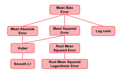
Figure 2. Schematic overview of the regression losses showing the connection

Unformatted plain text less than 2000 characters long (including spaces)

All the losses considered for the regression task are based on functions of the residuals, i.e. the difference between the observed value $y$ and the predicted value $f(\mathbf{x})$. In the following, let $f(\mathbf{x}_{i})$ be the outcome of the prediction over $\mathbf{x}_{i}$, and $y$ be the ground truth of the $i^{th}$ variable of interest.

As highlighted by Fig. 2 the Mean Bias Error ($MBE$) loss can be considered a base pillar for regression losses, characterized by many variations. Among them the most relevant are: Mean Absolute Error ($MAE$), Mean Squared Error ($MSE$), and Root Mean Squared Error ($RMSE$) losses. In this section we are also going to introduce the Huber loss and the smooth L1, which are a blend between the $MAE$ and the $MSE$. Finally, the Log-cosh and the Root Mean Squared Logarithmic Error losses are presented.

4.0.1. Mean Bias Error Loss (CONT, DIFF)

The most straightforward loss function is the Mean Bias Error loss, illustrated in Equation 8. It captures the average bias in the prediction, but is rarely adopted as loss function to train regression models, because positive errors may cancel out the negative ones, leading to a potential erroneous estimation of the parameters. Nevertheless, it is the starting point of the loss functions defined in the next subsections and it is commonly used to evaluate the performances of the models (Ullah et al., 2019; Krishnaiah et al., 2007; Valipour et al., 2013).

(8) $$\mathcal{L}_{MBE}=\frac{1}{N}\sum_{i=1}^{N}y_{i}-f(\mathbf{x}_{i})$$

Directly connected to $MBE$ there are respectively the Mean Absolute Error, the Mean Squared Error and the Log-cosh losses, which basically differs from $MBE$ in how they exploit the bias.

4.0.2. Mean Absolute Error Loss (L-CONT,CONV)

The Mean Absolute Error loss or L1 loss is one of the most basic loss functions for regression, it measures the average of the absolute bias in the prediction. The absolute value overcomes the problem of the $MBE$ ensuring that positive errors do not cancel the negative ones. Therefore each error contributes to $MAE$ in proportion to the absolute value of the error. Notice that, the contribution of the errors follows a linear behavior, meaning that many small errors are important as a big one. This implies that the gradient magnitude is not dependent on the error size, thus may leading into convergence problems when the error is small. A model trained to minimize the MAE is more effective when the target data conditioned on the input is symmetric. It is important to highlight that the derivative of the absolute value at zero is not defined.

As for MBE, MAE is also used to evaluate the performances of the models (Willmott and Matsuura, 2005; Li and Shi, 2010).

(9) $$\mathcal{L}_{MAE}=\frac{1}{N}\sum_{i=1}^{N}\left|y_{i}-f(\mathbf{x}_{i})\right|$$

4.0.3. Mean Squared Error Loss (CONT, DIFF, CONV)

The Mean Squared Error loss, or L2 loss, is the average of squared distances between the observed value $y$ and the predicted value $\hat{y}$. As for $MAE$, it is a well-known and straightforward loss function for regression. The squared term makes all the biases positive and magnifies the contribution made by outliers, making it more suitable for problems where noise in the observations follows a normal distribution. The main drawback is the sensitivity to the outliers.

(10) $$\mathcal{L}_{MSE}=\frac{1}{N}\sum_{i=1}^{N}\left(y_{i}-f(\mathbf{x}_{i})\right)^{2}$$

4.0.4. Root Mean Squared Error Loss(CONT,DIFF,CONV)

Directly connected to MSE, we have the Root Mean Squared Error loss, which is similar to MSE except for the square root term. The main advantage is to make sure that the loss has the same units and scale of the variable of interest. Since the only difference between the MSE and the RMSE consists in the application of the root term, the minimization process converge to the same optimal value. However, depending on the optimisation technique used, the RMSE may take different gradient steps. As the previously presented loss functions, it is also used as a metric to compare the performances of the model (Valipour et al., 2013; Li and Shi, 2010), and it shares the same limitations.

(11) $$\mathcal{L}_{RMSE}=\sqrt{\frac{1}{N}\sum_{i=1}^{N}\left(y_{i}-f(\mathbf{x}_{i})\right)^{2}}$$

4.0.5. Huber loss (L-CONT,DIFF,S-CONV)

The Huber loss (Huber, 1965) is a variant of the MAE that becomes MSE when the residuals are small. It is parameterized by $\delta$, which defines the transition point from MAE to MSE. When $\left|\mathbf{y_{i}}-f(\mathbf{x_{i}})\right|\leq\delta$ the Huber loss follows the MSE, otherwise it follows the MAE. This allows it to combine the advantages of both the MAE and the MSE, when the difference between the prediction and the output of the model is huge errors are linear, make the Huber loss less sensitive to the outliers. Conversely, when the error is small, it follows the MSE making the convergence much faster and differentiable at 0. The choice of $\delta$ is fundamental and it can be constantly adjusted during the training procedure based on what is considered an outlier. The main limitation of the Huber loss resides in the additional extra hyperparameter $\delta$.

(12) $$L_{Huberloss}=\left\{\begin{matrix}\frac{1}{2}\left(y_{i}-f(\mathbf{x}_{i})\right)^{2}&for\left|y_{i}-f(\mathbf{x}_{i})\right|\leq\delta,\\ \delta\left(\left|y_{i}-f(\mathbf{x}_{i})\right|-\frac{1}{2}\delta\right)&otherwise\end{matrix}\right.$$

Notice that, when $\delta=1$, we obtain the smooth L1 loss.

4.0.6. Log-cosh loss(CONT, DIFF)

The log-cosh loss is the logarithm of the hyperbolic cosine of the residuals between the observed value $y$ and the predicted value $\hat{y}$. It has all the advantages of the Huber loss, without the requirement of setting a hyperparameter, at the cost of being more computationally expensive. Furthermore, another benefit of the log-cosh loss is related to the fact that is differentiable twice everywhere, making it suitable for methods that requires solving the second derivative. As $log\left(cosh\left(\mathbf{x}\right)\right)$ is approximately equal to $\frac{\mathbf{x}^{2}}{2}$ for small values of $\mathbf{x}$ it behave similarly to the MSE. For larger value of $\mathbf{x}$ instead, is nearly equivalent to $\left|\mathbf{x}\right|-log\left(2\right)$ making it similar to MAE.

(13) $$\mathcal{L}_{logcosh}=\frac{1}{N}\sum_{i=1}^{N}log\left(cosh\left(f(\mathbf{x}_{i})-y_{i}\right)\right)$$

Another drawback of $\mathcal{L}_{logcosh}$ is related to the fact that, compared to the Huber loss, it is less customizable.

4.0.7. Root Mean Squared Logarithmic Error Loss(CONT,DIFF,CONV)

The Root Mean Squared Logarithmic Error (RMSLE) loss (formalized in Eq. 14) is the RMSE of the log-transformed observed value $y$ and log-transformed predicted value $\hat{y}$. The only difference with respect to RMSE is that the logarithm is applied to both the predicted and the observed values. The plus one term inside the logarithm allows values of $f(\mathbf{x}_{i})$ to be zero.

Due to the properties of the logarithm, the error between the predicted and the actual values is relative, making the RMSLE more robust to outliers. Precisely, the magnitude of the RMLSE does not scale accordingly to the magnitude of the error. Indeed, data points with big residuals are less penalized when the predicted and the actual values have high values too. This make the RMSLE suitable for problems where targets have an exponential relationship, or it is preferable to penalize more under estimates than over estimates. However, this loss is not appropriate for problems that allows negative values.

(14) $$\mathcal{L}_{RMSLE}=\sqrt{\frac{1}{N}\sum_{i=1}^{N}\left(\log(y_{i}+1)-\log(f(\mathbf{x}_{i})+1)\right)^{2}}$$

5. Classification losses

5.1. Problem Formulation and Notation

Classification is a subset of problems belonging to supervised learning. The goal is to assign an input $\mathbf{x}$ to one of $K$ discrete classes. This goal can be pursued by training a model $f_{\mathbf{\Theta}}$ and its parameters $\mathbf{\Theta}$ by minimizing a loss function $L$. Let the target space of $f$ discrete and consider a model returning the output label, $f$ can be defined as:

$$f\colon \Phi\to\Lambda^{K}$$

$$\Lambda=\{0,1\}$$

The above definition is working also for multi-label classification, since more than one label could be associated to a sample, e.g. $f(\mathbf{x})=[0,1,0,1,0,0]$. In order to define single label classification we need to add the constraint that the output sum up to $1$, $\sum_{k}\lambda_{k}=1$.
We can also consider models with continuous outputs, in case they return a probability $p_{k}(\mathbf{x})\in[0,1]$ to a sample $\mathbf{x}$ for each possible assignable label $k\in 1,...,K$:

$$f\colon \Phi\to P^{K}$$

$$P=[0,1]$$

As before, to switch between multi-label and single-label classification, we need to constraint the probabilities output to sum up to one, $\sum_{k}p_{k}=1$, if we want to force a single label assignment.

A more narrow notation for classification can be introduced in order to describe binary classification problems. This notation is useful in this work because margin based losses are designed to solve binary classification problems and cannot be generalised to multi-class or multi label classification. For the subset of binary classification problems the target space of $f$ is discrete and it is defined as follows:

$$f\colon \Phi\to B$$

$$B=\{-1,1\}$$

We define two different macro categories of classification losses accordingly to the underlying strategy employed to optimize them, namely the margin based and the probabilistic ones as illustrated in Fig. 3. In the next section, we introduce the margin based loss function starting by the most basic and intuitive one, the Zero-One loss. Subsequently, we present the Hinge loss and its variants (the Smoothed and Quadratically Smoothed Hinge losses). Then, the Modified Huber loss, the Ramp loss, and the Cosine Similarity loss are described. Moreover, we introduce the probabilistic loss by introducing the Cross Entropy loss and Negative Log-Likelihood loss, which, from a mathematical point of view, coincides. Finally, the Kullback-Leibler Divergence loss is presented.

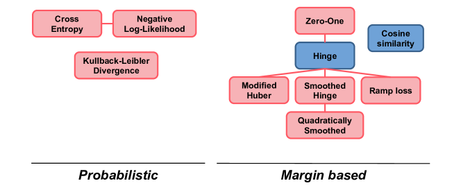
Figure 3. Overview of the classification losses divided in two major groups: margin based losses and probabilistic ones.

5.2. Margin Based Loss Functions

In this section, we introduce the most known margin based loss functions.

5.2.1. Zero-One loss

The basic and more intuitive margin based classification loss is the Zero-One loss. It assigns 1 to a misclassified observation and 0 to a correctly classified one.

(15) $$L_{\text{ZeroOne}}(f(\mathbf{x}),y)=\begin{cases}1&\text{if $f(\mathbf{x})\cdot y<0$}\\ 0&\text{otherwise}\end{cases}$$

ZeroOne loss is not directly usable since it lacks convexity and differentiability. However, it is possible to derive employable surrogate losses that are classification calibrated, which means that they are a relaxation of $L_{ZeroOne}$, or an upper bound, or an approximation of such loss. A significant achievement of the recent literature on binary classification has been the identification of necessary and sufficient conditions under which such relaxations yield Fisher consistency (Bartlett et al., 2006; Jiang, 2004; Lugosi and Vayatis, 2003; Mannor et al., 2003; Steinwart, 2005; Zhang, 2001). All the following losses satisfy such conditions.

5.2.2. Hinge loss and Perceptron loss (L-CONT,CONV)

The most famous surrogated loss is the Hinge loss (Gentile and Warmuth, 1998), which linearly penalizes every prediction where the resulting agreement is $<=1$.

(16) $$L_{\text{Hinge}}(f(\mathbf{x}),y)=\max(0,1-(f(\mathbf{x})\cdot y))$$

The Hinge loss is not strictly convex, but it is Lipschitz continuous and convex, so many of the usual convex optimizers used in machine learning can work with it. The Hinge loss is commonly employed to optimise the Support Vector Machine (SVM (Boser et al., [n. d.]; Mathur and Foody, 2008)).

To train the Perceptron (Rosenblatt, 1958) a variation of this loss, the Perceptron loss, is employed. This loss slightly differs from the Hinge loss, because it does not penalise samples inside the margin, surrounding the separating hyperplane, but just the ones that are mislabeled by this hyperplane with the same linear penalisation.

(17) $$L_{\text{Perceptron}}(f(\mathbf{x}),y)=\max(0,-(f(\mathbf{x})\cdot y))$$

There are two main drawbacks using the hinge loss. Firstly, its adoption use to make the model sensible to outliers in the training data. Secondly, due to the discontinuity of the derivative at $(f(\mathbf{x})\cdot y)=1$, i.e. the fact that is not continuously differentiable, Hinge loss results difficult to optimise.

5.2.3. Smoothed Hinge loss (L-CONT,CONV)

A smoothed version of the Hinge loss was defined in (Rennie, 2013) with the goal of obtaining a function easier to optimise as shown by the following equation:

(18) $$L_{\text{SmoothedHinge}}(f(\mathbf{x}),y)=\begin{cases}\frac{1}{2}-(f(\mathbf{x})\cdot t)&(f(\mathbf{x})\cdot y)<=0\\ \frac{1}{2}(1-(f(\mathbf{x})\cdot t))^{2}&0<(f(\mathbf{x})\cdot y)<1\\ 0&(f(\mathbf{x})\cdot y)>=1\end{cases}$$

This smoothed version of the Hinge loss is differentiable. Clearly, this is not the only possible smooth version of the Hinge loss. However, it is a canonical one that has the important property of being zero for $z>=1$ and it has constant (negative) slope for $z<=0$. Moreover, for $0<z<1$, the loss smoothly transitions from zero slope to a constant negative one. This loss inherit sensibility to outliers from the original Hinge loss.

5.2.4. Quadratically Smoothed Hinge loss (L-CONT,CONV,DIFF)

With the same goal of the Smoothed Hinge loss a quadratically smoothed version has been defined in (Zhang, 2004), to make it easier to be optimised:

(19) $$L_{\text{QSmoothedHinge}}(f(\mathbf{x}),y)=\begin{cases}\frac{1}{2\gamma}\max(0,-(f(\mathbf{x})\cdot y))^{2}&(f(\mathbf{x})\cdot y)>=1-\gamma\\ 1-\frac{\gamma}{2}-(f(\mathbf{x})\cdot y)&\text{otherwise}\end{cases}$$

The hyperparameter $\gamma$ determines the degree of smoothing, for $\gamma\rightarrow 0$ the loss becomes the original hinge. In contrast with the Smoothed Hinge loss, this version is not differentiable in the whole domain.

5.2.5. Modified Huber loss (L-CONT, DIFF, S-CONV)

The Modified Huber loss is a slight variation of the Huber loss for regression and a special case of the Quadratic Smoothed Hinge loss with $\gamma=2$ (For more details refer to section 4.0.5):

(20) $$L_{\text{ModHuber}}(f(\mathbf{x}),y)=\begin{cases}\frac{1}{4}\max(0,-(f(\mathbf{x})\cdot y))^{2}&(f(\mathbf{x})\cdot y)>=-1\\ -(f(\mathbf{x})\cdot y)&\text{otherwise}\end{cases}$$

5.2.6. Ramp loss (CONT,CONV)

The Ramp loss, or Truncated Hinge, is a piece-wise linear, continuous and convex loss that has been presented in (Wu and Liu, 2007). Under multi-class setting, this loss is more robust to outliers. When employed in SVM, it produces more accurate classifiers using a smaller, and more stable, set of support vectors than the multi-class SVM that employes $L_{\text{Hinge}}$ (Lee et al., 2002), also preserving fisher consistency.

(21) $$L_{\text{Ramp}}(f(\mathbf{x}),y)=\begin{cases}L_{\text{Hinge}}(f(\mathbf{x}),y))&(f(\mathbf{x})\cdot y)<=1\\ 1&\text{otherwise}\end{cases}$$

5.2.7. Cosine Similarity loss (L-CONT,DIFF)

Cosine similarity is generally used as a metric to measure distance when the magnitude of vectors is not important (Bishop and Nasrabadi, 2006). A typical example is related to text data representation by means of word counts (Mitchell and Mitchell, 1997; Bishop and Nasrabadi, 2006). When the label and output can be interpreted as vectors it is possible to derive a distance metric between them, which can be adapted into a loss function as follows:

(22) $$L_{cos-sim}(f(\mathbf{x}),\mathbf{y})=1-\frac{\mathbf{y}\cdot\mathbf{f(x)}}{\left\lVert\mathbf{y}\right\rVert\left\lVert\mathbf{f(x)}\right\rVert}$$

It is important to underline that, when using Cosine Similarity loss, the range of possible values is restricted to the interval [-1, 1], which may not be suitable for all types of data or applications, particularly when interpretability is a key requirement.

5.3. Probabilistic loss Functions

Let $q$ be the probability distribution underlying the dataset and $f_{\mathbf{\Theta}}$ the function generating the output, probabilistic loss functions provide some distance function between $q$ and $f_{\mathbf{\Theta}}$. By minimizing that distance, the model output distribution converges to the ground truth one. Usually, models trained with probabilistic loss functions can provide a measure of how likely a sample is labeled with one class instead of another (Mitchell and Mitchell, 1997; Bishop and Nasrabadi, 2006; Harshvardhan et al., 2020) providing richer information w.r.t. margin based .

5.3.1. Cross Entropy loss and Negative Log-Likelihood loss (CONT,DIFF,CONV)

Maximum likelihood estimation (MLE) is a method to estimate the parameters of a probability distribution by maximizing the likelihood (Mitchell and Mitchell, 1997; Bishop and Nasrabadi, 2006; Myung, 2003). From the point of view of Bayesian inference, MLE can be considered a special case of maximum a-posteriori estimation (MAP) that assumes a uniform prior distribution of the parameters. Formally, it means that, given a dataset of samples $\mathcal{D}$, we are maximizing the following quantity:

(23) $$P(\mathcal{D}|\mathbf{\Theta})=\prod_{n=1}^{N}f_{\mathbf{\Theta}}(\mathbf{x}_{i})^{y_{i}}\cdot(1-f_{\mathbf{\Theta}}(\mathbf{x}_{i}))^{1-y_{i}}$$

The aim is to find the maximum likelihood estimate by minimizing a loss function. To maximize Eq. 23, we can turn it into a minimisation problem by employing the negative log likelihood. To achieve this goal we need to define the following quantity:

(24) $$log(P(\mathcal{D}|\mathbf{\Theta}))=\sum_{i=1}^{N}(y_{i}\log(f_{\mathbf{\Theta}}(\mathbf{x}_{i}))+(1-y_{i})\log(1-f_{\mathbf{\Theta}}(\mathbf{x}_{i}))))$$

and we can obtain the loss function by taking the negative of the log:

(25) $$\mathcal{L}_{NLL}=-\sum_{i=1}^{N}(y_{i}\log(f_{\mathbf{\Theta}}(\mathbf{x}_{i}))+(1-y_{i})\log(1-f_{\mathbf{\Theta}}(\mathbf{x}_{i})))$$

Often, the above loss is also called the cross-entropy loss, because it can be derived by minimising the cross entropy between $f_{\mathbf{\Theta}}$ and $q$.

(26) $$H(q,f_{\mathbf{\Theta}})=-\int q(\mathbf{x})\log(f_{\mathbf{\Theta}}(\mathbf{x}))d\mathbf{x}$$

For the discrete case (which is the one we are interested in) the definition of the cross entropy is:

(27) $$H(q,f_{\mathbf{\Theta}})=-\sum_{i=1}^{N}q(\mathbf{x}_{i})\log(f_{\mathbf{\Theta}}(\mathbf{x}_{i}))$$

Maximizing the likelihood with respect to the parameters $\mathbf{\Theta}$ is the same as minimizing the cross-entropy as shown by the following equations:

(28) $$\sum_{i=1}^{N}(y_{i}\log(f_{\mathbf{\Theta}}(\mathbf{x}_{i}))+(1-y_{i})\log(1-f_{\mathbf{\Theta}}(\mathbf{x}_{i})))= \frac{1}{N}\prod_{n=1}^{N}f_{\mathbf{\Theta}}(\mathbf{x}_{i})^{Ny_{i}}$$

(29) $$= \sum_{i=1}^{N}q(\mathbf{x}_{i})\log(f_{\mathbf{\Theta}}(\mathbf{x}_{i})$$

(30) $$= -H(q,f_{\mathbf{\Theta}})$$

The classical approach to extend this loss to the multi-class scenario is to add as a final activation of the model a softmax function, defined accordingly to the number of ($K$) classes considered. Given a score for each class $f_{k}(\mathbf{x})=s$, it’s output can be squashed to sum up to $1$ by mean of a softmax function $f_{S}$ obtaining:

(31) $$\widehat{f}_{k}(\mathbf{x}_{i})=f_{S}(f_{k}(\mathbf{x}))$$

where, the softmax is defined as follows:

(32) $$f_{S}(s_{i})=\frac{e^{s_{i}}}{\sum_{j=1}^{K}e^{s_{j}}}$$

The final loss (usually named as categorical cross entropy) is:

(33) $$L_{CCE}=-\frac{1}{K}\sum_{j=1}^{K}\log(\widehat{f}_{k}(\mathbf{x}))$$

5.3.2. Kullback-Leibler divergence (CONT, CONV, DIFF)

The Kullback-Leibler (KL) divergence is an information-based measure of disparity among probability distributions. Precisely, it is a non-symmetrical measurement of how one probability distribution differs from another one (Joyce, 2011; Mitchell and Mitchell, 1997; Bishop and Nasrabadi, 2006). Technically speaking, KL divergence is not a distance metric because it doesn’t obey to the triangle inequality ($KL(q||f_{\mathbf{\Theta}})$ is not equal to $KL(f_{\mathbf{\Theta}}||q)$). It is important to notice that, in the classification use case, minimizing the KL divergence is the same as minimising the cross entropy. Precisely, the KL between two continuous distributions is defined as:

(34) $$\text{KL}(q||f_{\mathbf{\Theta}})=\int q(\mathbf{x})\log(\frac{q(\mathbf{x})}{f_{\mathbf{\Theta}}(\mathbf{x})})d\mathbf{x}=-\int q(\mathbf{x})\log(f_{\mathbf{\Theta}}(\mathbf{x}))d\mathbf{x}+\int q(\mathbf{x})\log(q(\mathbf{x}))d\mathbf{x}$$

If we want to minimise KL on the parameter $\mathbf{\Theta}$, since the second integral is non-dependant on $\mathbf{\Theta}$, we obtain:

(35) $$\min_{\mathbf{\Theta}}\text{KL}(q||f_{\mathbf{\Theta}})=\min_{\mathbf{\Theta}}-\int q(\mathbf{x})\log(f_{\mathbf{\Theta}}(\mathbf{x}))d\mathbf{x}=\min_{\mathbf{\Theta}}H(q,f_{\mathbf{\Theta}})$$

In general, it is preferable using cross entropy, instead of KL divergence, because it is typically easier to compute and optimize. The cross entropy only involves a single sum over the data, whereas the KL divergence involves a double sum. This can make it more computationally efficient, especially when working with large datasets.

6. Generative losses

In recent years, generative models have become particularly useful for both understanding the complexity of data distributions and being able to regenerate them (Goodfellow et al., 2020; Goodfellow et al., 2014a). In this section, as shown in the Fig. 4, we describe the losses relevant to Generative Adversarial Networks (GANs) and Diffusion Models. However, generative models are not limited to these cases, but extend to include more models. For example, Variational Auto-Encoders (VAEs) (Pu et al., 2016; An and Cho, 2015; Kingma and Welling, 2013) in which the KL-divergence, described in section 5.3.2, is the loss function employed. The objective of the VAE loss is to reduce the discrepancy between the original distribution and its predicted distribution. Other models such as the pixel recurrent neural networks (Van Oord et al., 2016) and real-valued Non-Volume Preserving (realNVP) models (Dinh et al., 2016) are not considered in this survey.

Figure 4. Overview of the generative losses.

6.1. Generative Adversarial Networks

Generative Adversarial Networks (GANs) are used to create new data instances that are sampled from the training data. GANs have two main components:

• The generator, referred as $G(\{\mathbf{z}_{0},\cdots,\mathbf{z}_{N}\})$, which generates data starting from random noise and tries to replicate real data distributions

• The discriminator, referred as $D(\{\mathbf{x}_{0},\cdots,\mathbf{x}_{N}\})$, which learns to distinguish the generator’s fake data from real one. It applies penalties in the generator loss for producing distinguishable fake data compared with real data.

The GAN architecture is relatively straightforward, although one aspect remains challenging: GAN loss functions. Precisely, the discriminator is trained to provide the loss function for the generator. If generator training goes well, the discriminator gets worse at telling the difference between real and fake samples. It starts to classify fake data as real, and its accuracy decreases.

Both the generator and the discriminator components are typically neural networks, where the generator output is connected directly to the discriminator input. The discriminator’s classification provides a signal that the generator uses to update its weights through back-propagation.

As GANs try to replicate a probability distribution, they should use loss functions that reflect the distance between the distribution of the data generated by the GAN and the distribution of the real data.

Two common GAN loss functions are typically used: minimax loss (Goodfellow et al., 2014b) and Wasserstein loss (Arjovsky et al., 2017). The generator and discriminator losses derive from a single distance measure between the two aforementioned probability distributions. The generator can only affect one term in the distance measure: the term that reflects the distribution of the fake data. During generator training, we drop the other term, which reflects the real data distribution. The generator and discriminator losses look different, even though they derive from a single formula.

In the following, both minimax and Wasserstein losses are written in a general form. The properties of the loss function (CONT, DIFF, etc.) are identified based on the function chosen for the generator or discriminator.

6.1.1. Minimax loss

The generative model $G$ learns the data distributions and is trained simultaneously with the discriminative model $D$. The latter estimates the probability that a given sample is identical to the training data rather than $G$. $G$ is trained to maximize the likelihood of tricking $D$ (Goodfellow et al., 2014b). In other words, the generator tries to minimize the following function while the discriminator tries to maximize it:

(36) $$\mathcal{L}_{minimax}(D,G)=E_{\{\mathbf{x}_{0},\cdots,\mathbf{x}_{N}\}}[\log(D(\{\mathbf{x}_{0},\cdots,\mathbf{x}_{N}\}))]+E_{\{\mathbf{z}_{0},\cdots,\mathbf{z}_{N}\}}[\log(1-D(G(\{\mathbf{z}_{0},\cdots,\mathbf{z}_{N}\})))],$$

where:

• $D(\{\mathbf{x}_{0},\cdots,\mathbf{x}_{N}\})$ is the discriminator’s estimate of the probability that real data instance {$\mathbf{x}_{0},\cdots,\mathbf{x}_{N}$} is real,

• $E_{\{\mathbf{x}_{0},\cdots,\mathbf{x}_{N}\}}$ is the expected value over all real data instances,

• $G(\{\mathbf{z}_{0},\cdots,\mathbf{z}_{N}\})$ is the generator’s output when given noise $\{\mathbf{z}_{0},\cdots,\mathbf{z}_{N}\}$,

• $D(G(z))$ is the discriminator’s estimate of the probability that a fake instance is real,

• $E_{\{\mathbf{z}_{0},\cdots,\mathbf{z}_{N}\}}$ is the expected value over all random inputs to the generator (in effect, the expected value over all generated fake instances $G(\{\mathbf{z}_{0},\cdots,\mathbf{z}_{N}\}))$.

The loss function above directly represents the cross-entropy between real and generated data distributions. The generator can’t directly affect the $\log(D(\{\mathbf{x}_{0},\cdots,\mathbf{x}_{N}\}))$ term in the function, and it only minimizes the term $\log(1-D(G(\{\mathbf{z}_{0},\cdots,\mathbf{z}_{N}\})))$. A disadvantage of this formulation of the loss function is that the above minimax loss function can cause the GAN to get stuck in the early stages of the training when the discriminator received trivial tasks. Therefore, a suggested modification to the loss (Goodfellow et al., 2014b) is to allow the generator to maximize $\log(D(G(\{\mathbf{z}_{0},\cdots,\mathbf{z}_{N}\})))$.

6.1.2. Wasserstein loss

The Wasserstein distance gives an alternative method of training the generator to better approximate the distribution of the training dataset. In this setup, the training of the generator itself is responsible for minimizing the distance between the distribution of the training and generated datasets. The possible solutions are to use distribution distance measures, like Kullback-Leibler (KL) divergence, Jensen-Shannon (JS) divergence, and the Earth-Mover (EM) distance (also called Wasserstein distance). The main advantage of using Wasserstein distance is due to its differentiability and having a continuous linear gradient (Arjovsky et al., 2017).

A GAN that uses a Wasserstein loss, known as a WGAN, does not discriminate between real and generated distributions in the same way as other GANs. Instead, the WGAN discriminator is called a ”critic,” and it scores each instance with a real-valued score rather than predicting the probability that it is fake. This score is calculated so that the distance between scores for real and fake data is maximised.

The advantage of the WGAN is that the training procedure is more stable and less sensitive to model architecture and selection of hyperparameters.

The two loss functions can be written as:

(37) $$\mathcal{L}_{critic}=D(\{\mathbf{x}_{0},\cdots,\mathbf{x}_{N}\})-D(G(\{\mathbf{z}_{0},\cdots,\mathbf{z}_{N}\})),~{}~{}~{}\mathcal{L}_{Generator}=D(G(\{\mathbf{z}_{0},\cdots,\mathbf{z}_{N}\}))$$

The discriminator tries to maximize $\mathcal{L}_{critic}$. In other words, it tries to maximize the difference between its output on real instances and its output on fake instances. The generator tries to maximize $\mathcal{L}_{Generator}$. In other words, It tries to maximize the discriminator’s output for its fake instances.

The benefit of Wasserstein loss is that it provides a useful gradient almost everywhere, allowing for the continued training of the models. It also means that a lower Wasserstein loss correlates with better generator image quality, meaning that it explicitly seeks a minimization of generator loss. Finally, it is less vulnerable to getting stuck in a local minimum than minimax-based GANs (Arjovsky et al., 2017). However, accurately estimating the Wasserstein distance using batches requires unaffordable batch size, which significantly increases the amount of data needed (Stanczuk et al., 2021).

6.2. Diffusion models

Diffusion Models are generative models that rely on probabilistic likelihood estimation to generate data samples. They were originally inspired by the physical phenomena called diffusion. Diffusion Modelling is a learning procedure in which a model can learn the systematic decay of information due to adding a slight noise factor iteratively (Sohl-Dickstein et al., 2015; Song and Ermon, 2019). The learning procedure enables the possibility of recovering the decayed information from the noise again. They model a series of noise distributions in a Markov Chain and they decode the original data by systematically removing the noises hierarchically (Ho et al., 2020; Ching and Ng, 2006).

The diffusion process consists of two steps, the forward process and the reconstruction (reverse) process. Gaussian noise is gradually added during the forward diffusion process until the data sample loses its distinguishable features. The reverse process removes the noise and restores the original data by utilizing a neural network model to learn the conditional probability densities.

6.2.1. Forward diffusion process

Given a data point $\mathbf{x_{0}}$ sampled from a real data distribution $q(\mathbf{x})$. The forward process aims to add a small noise iteratively $T$ times. For every data point $\mathbf{x_{0}}$ the process produces a sequence of noisy samples $\mathbf{x_{1}},\cdots,\mathbf{x_{T}}$. The noise distributions is usually chosen to be Gaussian. Because the forecast of probability density at time $t$ is only dependent on the immediate predecessor at time $t-1$, the conditional probability density can be calculated as:

(38) $$q(\mathbf{x}_{t}|\mathbf{x}_{t-1})=\mathcal{N}(\mathbf{x}_{t};\sqrt{1-\beta_{t}}\mathbf{x}_{t-1},\beta_{t}\mathbf{I})\quad q(\mathbf{x}_{1:T}|\mathbf{x}_{0})=\prod^{T}_{t=1}q(\mathbf{x}_{t}|\mathbf{x}_{t-1})$$

With a $\beta_{t}\in(0,1)$ is a hyperparameter that can be taken as constant or variable and $t\in[1,T]$. As $T\rightarrow\infty,\mathbf{x_{T}}$ becomes a pure Gaussian distribution. We can only sample the new states of the system using the gradient of the density function in Markov Chain updates, according to stochastic gradient Langevin dynamics (Welling and Teh, 2011). The following formula can then be employed to calculate the sampling of a new data point at time $t$ with a step size $\delta$ dependent on the prior point at time $t-1$:

(39) $$\mathbf{x}_{t}=\mathbf{x}_{t-1}+\frac{\delta}{2}\nabla_{\mathbf{x}}\log q(\mathbf{x}_{t-1})+\sqrt{\delta}\bm{\epsilon}_{t},\quad\text{where }\bm{\epsilon}_{t}\sim\mathcal{N}(\mathbf{0},\mathbf{I})$$

when $T\to\infty,\bm{\epsilon}\to 0$ equals to the true probability density $p(\mathbf{x})$. The forward step does not require training a neural network; it only requires an iterative process for adding random Gaussian noises to the original data distribution.

6.2.2. Reverse diffusion process

Given the system’s current state, the reverse process requires the calculation of probability density at a previous time step. Calculating the $q(\mathbf{x}_{t-1}|\mathbf{x}_{t})$ at the time $t=T$ is equal to producing data from an isotropic Gaussian noise. However, contrary to the forward process, the estimation of the past state from the present state requires the knowledge of every previous gradient, which is not feasible without the aid of a learning model that can forecast such estimates. This problem is resolved by training a neural network model that, using the learnt weights $\mathbf{\Theta}$ and the current state at time $t$, estimates the value of $p_{\mathbf{\Theta}}(\mathbf{x}_{t-1}|\mathbf{x}_{t})$ as formalized by the following equation:

(40) $$p_{\mathbf{\Theta}}(\mathbf{x}_{0:T})=p(\mathbf{x}_{T})\prod^{T}_{t=1}p_{\mathbf{\Theta}}(\mathbf{x}_{t-1}|\mathbf{x}_{t})\quad p_{\mathbf{\Theta}}(\mathbf{x}_{t-1}|\mathbf{x}_{t})=\mathcal{N}(\mathbf{x}_{t-1};\bm{\mu}_{\mathbf{\Theta}}(\mathbf{x}_{t},t),\bm{\Sigma}_{\mathbf{\Theta}}(\mathbf{x}_{t},t))$$

where $\bm{\mu}_{\mathbf{\Theta}}(\mathbf{x}_{t},t)$ is the mean function proposed in (Ho et al., 2020). The sample at time $t-1$ can then be computed as:

(41) $$\mathbf{x}_{t-1}=\mathcal{N}(\mathbf{x}_{t-1};\frac{1}{\sqrt{\alpha_{t}}}\Big{(}\mathbf{x}_{t}-\frac{1-\alpha_{t}}{\sqrt{1-\bar{\alpha}_{t}}}\bm{\epsilon}_{\mathbf{\Theta}}(\mathbf{x}_{t},t)\Big{)},\bm{\Sigma}_{\mathbf{\Theta}}(\mathbf{x}_{t},t))$$

6.2.3. Diffusion model loss function (CONT, DIFF)

The main task of the network model is to minimize the following loss:

(42) $$L_{diffusion}=\mathbb{E}_{t}\Big{[}\log p(\mathbf{x}_{T})-\sum_{t\geq 1}{\log\frac{p_{\mathbf{\Theta}}(\mathbf{x}_{t-1}|\mathbf{x}_{t})}{q(\mathbf{x}_{t}|\mathbf{x}_{t-1})}\Big{]}}$$

In (Sohl-Dickstein et al., 2015; Ho et al., 2020), it is shown that a simplified version of $L_{diffusion}$ is able to achieve better results:

(43) $$L_{diffusion}^{\text{simple}}=\mathbb{E}_{t\sim[1,T],\mathbf{x}_{0},\bm{\epsilon}_{t}}\Big{[}\|\bm{\epsilon}_{t}-\bm{\epsilon}_{\mathbf{\Theta}}(\sqrt{\bar{\alpha}_{t}}\mathbf{x}_{0}+\sqrt{1-\bar{\alpha}_{t}}\bm{\epsilon}_{t},t)\|^{2}\Big{]}$$

It is important to notice that diffusion Models perform significantly better in some applications despite being computationally more expensive than alternative deep network structures (Dhariwal and Nichol, 2021; Song and Ermon, 2020; Ho et al., 2022; Ramesh et al., 2022; Saharia et al., [n. d.]; Rombach et al., 2022).

7. Ranking losses

Machine learning can be employed to solve ranking problems, which have important industrial applications, especially in information retrieval systems. These problems can be typically solved by employing supervised, semi-supervised, or reinforcement learning (Bromley et al., 1993; Hoffer and Ailon, 2015).

The goal of ranking losses, in contrast to other loss functions like the cross-entropy loss or MSE loss, is to anticipate the relative distances between inputs rather than learning to predict a label, a value, or a set of values given an input. This is also sometimes called metric learning. Nevertheless, the cross-entropy loss can be used in the top-one probability ranking. In this scenario, given the scores of all the objects, the top-one probability of an object in this model indicates the likelihood that it will be ranked first (Cao et al., 2007).

Ranking loss functions for training data can be highly customizable because they require only a method to measure the similarity between two data points, i.e., similarity score. For example, consider a face verification dataset, pairs of photographs which belong to the same person will have a high similarity score, whereas those that don’t will have a low score  (Wang et al., 2014).

In general, ranking loss functions require a feature extraction for two (or three) data instances, which returns an embedded representation for each of them. A metric function can then be defined to measure the similarity between those representations, such as the euclidean distance. Finally, the feature extractors are trained to produce similar representations for both inputs in case the inputs are similar or distant representations in case of dissimilarity.

Similar to Section 6, both pairwise and triplet ranking losses are presented in a general form, as shown in the Fig. 5. The properties of the loss function (CONT, DIFF, etc.) are identified based on the metric function chosen.

Figure 5. Overview of the ranking losses.

7.1. Pairwise Ranking loss

In the context of Pairwise Ranking loss, positive and negative pairs of training data points are used  (Bromley et al., 1993; Chopra et al., 2005; Hadsell et al., 2006; Li et al., 2017). Positive pairs are composed of an anchor sample $\mathbf{x}_{a}$ and a positive sample $\mathbf{x}_{p}$, which is similar to $\mathbf{x}_{a}$ in the metric. Negative pairs are composed of an anchor sample $\mathbf{x}_{a}$ and a negative sample $\mathbf{x}_{n}$, which is dissimilar to $\mathbf{x}_{a}$ in that metric. The objective is to learn representations with a small distance $d$ between them for positive pairs and a greater distance than some margin value $m$ for negative pairs. Pairwise Ranking loss forces representations to have a 0 distance for positive pairs and a distance greater than a margin for negative pairs.

Given $\mathbf{r}_{a}$, $\mathbf{r}_{p}$, and $\mathbf{r}_{n}$ the embedded representations (the output of a feature extractor) of the input samples $\mathbf{x}_{a}$, $\mathbf{x}_{p}$, $\mathbf{x}_{n}$ respectively and $d$ as a distance function the loss function can be written as:

(44) $${L}_{pairwise}=\begin{cases}d(\mathbf{r}_{a},\mathbf{r}_{b})&\text{if positive pair}\\ \max(0,m-d(\mathbf{r}_{a},\mathbf{r}_{n}))&\text{if negative pair}\end{cases}$$

For positive pairs, the loss will vanish if the distance between the embedding representations of the two elements in the pair is 0; instead, the loss will increase as the distance between the two representations increases. For negative pairs, the loss will vanish if the distance between the embedding representations of the two elements is greater than the margin $m$. However, if the distance is less than $m$, the loss will be positive, and the model parameters will be updated to provide representations for the two items that are farther apart. When the distance between $\mathbf{r}_{a}$ and $\mathbf{r}_{n}$ is 0, the loss value will be at most $m$. The purpose of the margin is to create representations for negative pairs that are far enough, thus implicitly stopping the training on these pairs and allowing the model to focus on more challenging ones. If $\mathbf{r}_{0}$ and $\mathbf{r}_{1}$ are the pair elements representations, $y$ is a binary flag equal to 0 for a negative pair and to 1 for a positive pair, and the distance $d$ is the euclidean distance:

(45) $${L}_{pairwise}(\mathbf{r}_{0},\mathbf{r}_{1},y)=y||\mathbf{r}_{0}-\mathbf{r}_{1}||+(1-y)\max(0,m-||\mathbf{r}_{0}-\mathbf{r}_{1}||)$$

Unlike typical classification learning, this loss requires more training data and time because it requires access to all the data of all potential pairs during training. Additionally, because training involves pairwise learning, it will output the binary distance from each class, which is more computationally expensive if there is incorrect classification (Koch et al., 2015).

7.2. Triplet Ranking loss

Employing triplets of training data instances instead of pairs can produce better performance  (Hoffer and Ailon, 2015; Wang et al., 2014; Chechik et al., 2010). The resultant loss is called Triplet Ranking loss. A triplet consists of an anchor sample $\mathbf{x}_{a}$, a positive sample $\mathbf{x}_{p}$, and a negative sample $\mathbf{x}_{n}$. The objective is that the distance between the anchor sample and the negative sample representations $d(\mathbf{r}_{a},\mathbf{r}_{n})$ is greater (and bigger than a margin $m$) than the distance between the anchor and positive representations $d(\mathbf{r}_{a},\mathbf{r}_{p})$. The same notation applies:

(46) $${L}_{triplet}(\mathbf{r}_{a},\mathbf{r}_{p},\mathbf{r}_{n})=\max(0,m+d(\mathbf{r}_{a},\mathbf{r}_{p})-d(\mathbf{r}_{a},\mathbf{r}_{n}))$$

This loss is characterized by three different scenarios based on the values of $\mathbf{r}_{a}$, $\mathbf{r}_{p}$, $\mathbf{r}_{n}$, and $m$:

• Easy Triplets: $d(\mathbf{r}_{a},\mathbf{r}_{n})>d(\mathbf{r}_{a},\mathbf{r}_{p})+m$. In the embedding space, the distance between the negative sample and the anchor sample is already large enough. The model parameters are not changed, and the loss is $0$.

• Hard Triplets: $d(\mathbf{r}_{a},\mathbf{r}_{n})<d(\mathbf{r}_{a},\mathbf{r}_{p})$.Compared to the positive sample, the negative sample is closer to the anchor. The loss is positive (and $>m$). The model’s parameters are subject to change.

• Semi-Hard Triplets: $d(\mathbf{r}_{a},\mathbf{r}_{p})<d(\mathbf{r}_{a},\mathbf{r}_{n})<d(\mathbf{r}_{a},\mathbf{r}_{p})+m$. The loss is still positive (and $<m$) nevertheless, the negative sample is further away from the anchor than the positive sample. The model’s parameters are subject to change, and the loss is not $0$.

This loss is sensitive to small changes in the input samples, so it cannot be generalized. This means that once the model has been trained on a specific dataset, it cannot be applied to other datasets  (Koch et al., 2015).

8. Energy-based losses

An Energy-Based Model (EBM) is a probabilistic model that uses a scalar energy function to describe the dependencies of the model variables (LeCun et al., 2006; Friston et al., 2006; Friston, 2009; Finn et al., 2016; Haarnoja et al., 2017; Grathwohl et al., 2019; Du et al., 2019). An EBM can be formalised as ${F}:\mathcal{X}\times\mathcal{Y}\rightarrow\mathbb{R}$, where ${F}(\mathbf{x},\mathbf{y})$ stands for the relationship between the $(\mathbf{x},\mathbf{y})$ pairings.

Given an energy function and the input $\mathbf{x}$, the best fitting value of $\mathbf{y}$ is computed with the following inference procedure:

(47) $$\tilde{\mathbf{y}}=argmin_{\mathbf{y}}\{F(\mathbf{x},\{\mathbf{y}_{0},\cdots,\mathbf{y}_{N}\})\}$$

Energy-based models provide fully generative models that can be used as an alternative to probabilistic estimation for prediction, classification, or decision-making tasks (Osadchy et al., 2004; LeCun et al., 2006; Haarnoja et al., 2017; Du and Mordatch, 2019; Grathwohl et al., 2019).

The energy function $E(\mathbf{x},\mathbf{y})\equiv F(\mathbf{x},\mathbf{y})$ can be explicitly defined for all the values of $\mathbf{y}\in\mathcal{Y}=\{\mathbf{y}_{0},\cdots,\mathbf{y}_{N}\}$ if and only if the size of the set $\mathcal{Y}$ is small enough. In contrast, when the space of $\mathcal{Y}$ is sufficiently large, a specific strategy, known as the inference procedure, must be employed to find the $\mathbf{y}$ that minimizes $E(\mathbf{x},\{\mathbf{y}_{0},\cdots,\mathbf{y}_{N}\})$.

In many real situations, the inference procedure can produce an approximate result, which may or may not be the global minimum of $E(\mathbf{x},\{\mathbf{y}_{0},\cdots,\mathbf{y}_{N}\})$ for a given $\mathbf{x}$. Moreover, it is possible that $E(\mathbf{x},\{\mathbf{y}_{0},\cdots,\mathbf{y}_{N}\})$ has several equivalent minima. The best inference procedure to use often depends on the internal structure of the model. For example, if $\mathcal{Y}$ is continuous and $E(\mathbf{x},\{\mathbf{y}_{0},\cdots,\mathbf{y}_{N}\})$ is smooth and differentiable everywhere concerning $\mathbf{y}$, a gradient-based optimization algorithm can be employed  (Bengio, 2000).

In general, any probability density function $p(\mathbf{x})$ for $\mathbf{x}\in\mathbb{R}^{D}$ can be rewritten as an EBM:

(48) $$p_{\bm{\theta}}(\mathbf{x})=\frac{\exp(-E_{\bm{\theta}}(\mathbf{x}))}{\int_{\mathbf{x}’}\exp(-E_{\bm{\theta}}(\mathbf{x}’))d\mathbf{x}’},$$

where the energy function ($E_{\bm{\theta}}$) can be any function parameterised by ${\bm{\theta}}\in\mathbf{\Theta}$ (such as a neural network). In these models, a prediction (e.g. finding $p(\mathbf{x_{0}}|\mathbf{x_{1}},\mathbf{x_{2}},...)$) is done by fixing the values of the conditional variables, and estimating the remaining variables, (e.g. $\mathbf{x_{0}}$), by minimizing the energy function (Teh et al., 2003; Swersky et al., 2011; Zhai et al., 2016).

An EBM is trained by finding an energy function that associates low energies to values of $\mathbf{x}$ drawn from the underlying data distribution, $p_{\theta}(\mathbf{x})\sim p_{D}(\mathbf{x})$, and high energies for values of $\mathbf{x}$ not close to the underlying distribution.

8.1. Training

Given the aforementioned conceptual framework, the training can be thought as finding the model parameters that define the good match between the output ($\mathbf{y}\in\mathcal{Y}$) and the input ($\mathbf{x}\in\mathcal{X}$) for every step. This is done by estimating the best energy function from the set of energy functions ($\mathcal{E}$) by scanning all the model parameters $\mathbf{\mathbf{\Theta}}$ (Kumar et al., 2019; Song and Kingma, 2021), where $\mathcal{E}=\{F(\mathbf{\Theta},\mathbf{X},\mathbf{Y}):\mathbf{\Theta}\in\mathcal{W}=\mathbf{\Theta}\}$. A loss function should behave similarly to the energy function described in Equation 47, i.e., lower energy for a correct answer must be modeled by low losses, instead, higher energy, to all incorrect answers, by a higher loss.

Considering a set of training samples $\mathcal{S}=\{(\mathbf{x}_{i},\mathbf{y}_{i}):i=1,\cdots,N\}$, during the training procedure, the loss function should have the effect of pushing-down $E(\mathbf{\Theta},\mathbf{y}_{i},\mathbf{x}_{i})$ and pulling-up $E(\mathbf{\Theta},\tilde{\mathbf{y}}_{i},\mathbf{x}_{i})$, i.e., finding the parameters $\mathbf{\Theta}$ that minimize the loss:

(49) $$\mathbf{\Theta}^{*}=min_{\mathbf{\Theta}\in\mathcal{W}}L_{ebm}(\mathbf{\Theta},\mathcal{S})$$

The general form of the loss function $\mathcal{L}_{ebm}$ is defined as:

(50) $$\mathcal{L}_{ebm}(\mathbf{\Theta},\mathcal{S})=\frac{1}{N}\sum_{i=1}^{N}L_{ebm}(\mathbf{y}_{i},E(\mathbf{\Theta},\mathcal{Y},\mathbf{x}_{i}))+\text{regularizer term}$$

Where:

• $L_{ebm}(\mathbf{y}_{i},E(\mathbf{\Theta},\mathcal{Y},\mathbf{x}_{i}))$ is the per-sample loss

• $\mathbf{y}_{i}$ is the desired output

• $E(\mathbf{\Theta},\mathcal{Y},\mathbf{x}_{i}))$ is energy surface for a given $\mathbf{x}_{i}$ as $\mathbf{y}\in\mathcal{Y}$ varies

This is an average of a per-sample loss functional, denoted $L_{ebm}(\mathbf{y}_{i},E(\mathbf{\Theta},\mathcal{Y},\mathbf{x}_{i}))$, over the training set. This function depends on the desired output $\mathbf{y}_{i}$ and on the energies derived by holding the input sample $\mathbf{x}_{i}$ constant and changing the output scanning over the sample $\mathcal{Y}$. With this definition, the loss remains unchanged when the training samples are mixed up and when the training set is repeated numerous times (LeCun et al., 2006). As the size of the training set grows, the model is less likely to overfit (Vapnik, 1999).

8.2. Loss Functions for EBMs

Following Fig. 6, in this section, we introduce the energy loss first since it is the most straightforward. Then we present common losses in machine learning that can be adapted to the energy based models, such as the Negative Log-Likelihood loss, the Hinge loss, and the Log loss. Subsequently, we introduce more sophisticated losses like the Generalized Perceptron loss and the Generalized Margin loss. Finally, the Minimum classification error loss, the Square-square loss, and its variation Square-exponential loss are presented.

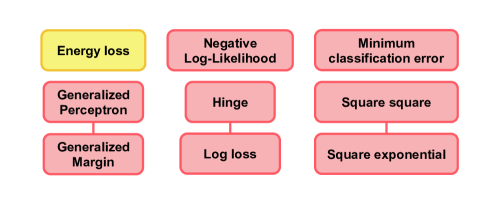
Figure 6. Schematic overview of the energy based losses with their connection.

8.2.1. Energy loss

The so-called energy loss is the most straightforward loss due to its simplicity. It can be simply defined by using the energy function as the per-sample loss:

(51) $${L}_{energy}(\mathbf{y}_{i},E(\mathbf{\Theta},\mathcal{Y},\mathbf{x}_{i}))=E(\mathbf{\Theta},\mathbf{x}_{i},\mathbf{y}_{i})$$

This loss is often used in regression tasks. Accordingly to its definition, it pulls the energy function down for values that are close to the correct data distribution. However, the energy function is not pulled up for incorrect values. The assumption is that, by lowering the energy function in the correct location, the energy for incorrect values is left higher as a result. Due to this assumption, the training is sensitive to the model design and may result in energy collapse, leading to a largely flat energy function.

8.2.2. Generalized Perceptron loss (L-CONT, CONV)

The Generalized Perceptron loss is defined as:

(52) $${L}_{perceptron}(\mathbf{y}_{i},E(\mathbf{\Theta},\mathcal{Y},\mathbf{x}_{i}))=E(\mathbf{\Theta},\mathbf{y}_{i},\mathbf{x}_{i})-[\min_{\mathbf{y}\in\mathcal{Y}}]\{E(\mathbf{\Theta},\{\mathbf{y}_{0},\cdots,\mathbf{y}_{N}\},\mathbf{x}_{i})\}$$

This loss is positive definite as the second term is the lower bound of the first one, i.e., $E(\mathbf{\Theta},\mathbf{y}_{i},\mathbf{x}_{i})-[min_{\mathbf{y}\in\mathcal{Y}}]\{E(\mathbf{\Theta},\{\mathbf{y}_{0},\cdots,\mathbf{y}_{N}\},\mathbf{x}_{i})\}\geq 0$. By minimizing this loss, the first term is pushed down and the energy of the model prediction is raised. Although it is widely used (LeCun et al., 1998; Collins, 2002), this loss is suboptimal as it does not detect the gap between the correct output and the incorrect ones, and it doesn’t restrict the function from assigning the same value to each wrong output $\mathbf{y}_{i}$ and it may produce flat energy distributions  (LeCun et al., 2006).

8.2.3. Negative Log-Likelihood loss (CONT,DIFF,CONV)

In analogy with the description in Section 5.3.1, the Negative Log-Likelihood loss (NLL) in the energy-based context is defined as:

(53) $$\mathcal{L}_{NLL}(\mathbf{\Theta},\mathcal{S})=\frac{1}{N}\sum_{i=1}^{N}\left(E(\mathbf{\Theta},\mathbf{y}_{i},\mathbf{x}_{i})+\frac{1}{\beta}\log\int_{\mathbf{y}\in\mathcal{Y}}e^{\beta E(\mathbf{\Theta},\mathbf{y},\mathbf{x}_{i})}\right)$$

where $\mathcal{S}$ is the training set.

This loss reduces to the perceptron loss when $\beta\rightarrow\infty$ and to the log loss in case $\mathcal{Y}$ has only two labels (i.e., binary classification). Since the integral above is intractable, considerable efforts have been devoted to finding approximation methods, including Monte-Carlo sampling methods (Shapiro, 2003), and variational methods (Jordan et al., 1999). While these methods have been devised as approximate ways of minimizing the NLL loss, they can be viewed in the energy-based framework as different strategies for choosing the $\mathbf{y}$’s whose energies will be pulled up (LeCun and Huang, 2005; LeCun et al., 2006). The NLL is also known as the cross-entropy (Levin and Fleisher, 1988) loss and is widely used in many applications, including energy-based models (Bengio et al., 2000, 1992). This loss function formulation is subject to the same limitations listed in section 5.3.1.

8.2.4. Generalized Margin loss

The generalized margin loss is a more reliable version of the generalized perceptron loss. The general form of the generalized margin loss in the context of energy-based training is defined as:

(54) $$L_{margin}(\mathbf{\Theta},\mathbf{x}_{i},\mathbf{y}_{i})={Q}_{m}(E(\mathbf{\Theta},\mathbf{x}_{i},\mathbf{y}_{i}),E(\mathbf{\Theta},\mathbf{x}_{i},\bar{\mathbf{y}}_{i}))$$

Where $\bar{\mathbf{y}}_{i}$ is the so-called ”most-offending incorrect output” which is the output that has the lowest energy among all possible outputs that are incorrect (LeCun et al., 2006), $m$ is a positive margin parameter, and $Q_{m}$ is a convex function which ensures that the loss receives low values for $E(\mathbf{\Theta},\mathbf{x}_{i},\mathbf{y}_{i})$ and high values for $E(\mathbf{\Theta},\mathbf{x}_{i},\bar{\mathbf{y}}_{i})$. In other words, the loss function can ensure that the energy of the most offending incorrect output is greater by some arbitrary margin than the energy of the correct output.

This loss function is written in the general form and a wide variety of losses that use specific margin function $Q_{m}$ to produce a gap between the correct output and the wrong output are formalised in the following part of the section.

Hinge loss (L-CONT,CONV)

Already explained in section 5.2.2, the hinge loss can be rewritten as:

(55) $$L_{hinge}(\mathbf{\Theta},\mathbf{x}_{i},\mathbf{y}_{i})=max(0,m+E(\mathbf{\Theta},\mathbf{x}_{i},\mathbf{y}_{i})-E(\mathbf{\Theta},\mathbf{x}_{i},\bar{\mathbf{y}}_{i}))$$

This loss enforces that the difference between the correct answer and the most offending incorrect answer be at least $m$ (Taskar et al., 2003; Altun et al., 2003). Individual energies are not required to take a specific value because the hinge loss depends on energy differences. This loss function shares limitations with the original Hinge loss defined in eq. 16.

Log loss (DIFF,CONT,CONV)

This loss is similar to the hinge loss, but it sets a softer margin between the correct output and the most offending outputs. The log loss is defined as:

(56) $$L_{log}(\mathbf{\Theta},\mathbf{x}_{i},\mathbf{y}_{i})=\log(1+e^{E(\mathbf{\Theta},\mathbf{x}_{i},\mathbf{y}_{i})-E(\mathbf{\Theta},\mathbf{x}_{i},\bar{\mathbf{y}}_{i})})$$

This loss is also called soft hinge and it may produce overfitting on high dimensional datasets  (Kleinbaum et al., 2002).

Minimum classification error loss (CONT, DIFF, CONV)

A straightforward function that roughly counts the total number of classification errors while being smooth and differentiable is known as the Minimum Classification Error (MCE) loss (Juang et al., 1997). The MCE is written as a sigmoid function:

(57) $$L_{mce}(\mathbf{\Theta},\mathbf{x}_{i},\mathbf{y}_{i})=\sigma(E(\mathbf{\Theta},\mathbf{x}_{i},\mathbf{y}_{i})-E(\mathbf{\Theta},\mathbf{x}_{i},\bar{\mathbf{y}}_{i}))$$

Where $\sigma$ is defined as $\sigma(x)=(1+e^{-x})^{-1}$. While this function lacks an explicit margin, it nevertheless produces an energy difference between the most offending incorrect output and the correct output.

Square-square loss (CONT,CONV)

Square-square loss deals differently with the energy of the correct output $E(\mathbf{\Theta},\mathbf{x}_{i},\mathbf{y}_{i})$ and the energy of the most offensive output $E(\mathbf{\Theta},\mathbf{x}_{i},\bar{\mathbf{y}}_{i})$ as:

(58) $$L_{sq-sq}(\mathbf{\Theta},\mathbf{x}_{i},\mathbf{y}_{i})=E(\mathbf{\Theta},\mathbf{x}_{i},\mathbf{y}_{i})^{2}+(\max(0,m-E(\mathbf{\Theta},\mathbf{x}_{i},\bar{\mathbf{y}}_{i})))^{2}$$

The combination aims to minimize the energy of the correct output while enforcing a margin of at least $m$ on the most offending incorrect outputs. This loss is a modified version of the margin loss. This loss can be only used when there is a lower bound on the energy function  (LeCun and Huang, 2005; Hadsell et al., 2006).

Square-exponential loss (CONT, DIFF, CONV)

This loss is similar to the square-square loss function, and it only differs in the second term:

(59) $$L_{sq-exp}(\mathbf{\Theta},\mathbf{x}_{i},\mathbf{y}_{i})=E(\mathbf{\Theta},\mathbf{x}_{i},\mathbf{y}_{i})^{2}+\gamma e^{-E(\mathbf{\Theta},\mathbf{x}_{i},\bar{\mathbf{y}}_{i})}$$

While $\gamma$ is a positive constant, the combination aims to minimize the energy of the correct output while pushing the energy of the most offending incorrect output to an infinite margin (LeCun and Huang, 2005; Chopra et al., 2005; Osadchy et al., 2004). This loss is considered a regularized version of the aforementioned square-square loss. This loss, as for the Square-square loss, can be only used when there is a lower bound on the energy function  (LeCun and Huang, 2005; Hadsell et al., 2006).

9. Conclusion

The definition of an appropriate loss function is a critical part of solving many machine learning problems. In this survey we have described 33 of the most commonly used loss functions from across the machine learning literature. These functions are appropriate for solving a wide range of problems, including classification, regression, sample generation and ranking. Overall, we made an effort to provide a useful resource for newcomers to the machine learning literature and advanced practitioners alike.

Each of the loss functions we describe have also been put into context and compared in a novel taxonomy, introduced in Sec. 2. This gives practitioners a quick view of the different techniques and how they fit together, allowing them to decide and choose the most appropriate approach for their technique quickly and efficiently. We also hope this framing helps researchers to contextualise newly developed loss functions.

References

- (1)
- Altun et al. (2003) Yasemin Altun, Ioannis Tsochantaridis, and Thomas Hofmann. 2003. Hidden markov support vector machines. In Proceedings of the 20th international conference on machine learning (ICML-03). 3–10.
- An and Cho (2015) Jinwon An and Sungzoon Cho. 2015. Variational autoencoder based anomaly detection using reconstruction probability. Special Lecture on IE 2, 1 (2015), 1–18.
- Argall et al. (2009) Brenna D Argall, Sonia Chernova, Manuela Veloso, and Brett Browning. 2009. A survey of robot learning from demonstration. Robotics and autonomous systems 57, 5 (2009), 469–483.
- Arjovsky et al. (2017) Martin Arjovsky, Soumith Chintala, and Léon Bottou. 2017. Wasserstein GAN. https://doi.org/10.48550/ARXIV.1701.07875
- Bartlett et al. (2002) Peter Bartlett, Stéphane Boucheron, and Gábor Lugosi. 2002. Model Selection and Error Estimation. Machine Learning 48 (01 2002), 85–113. https://doi.org/10.1023/A:1013999503812
- Bartlett et al. (2006) Peter L. Bartlett, Michael I. Jordan, and Jon D. McAuliffe. 2006. Convexity, Classification, and Risk Bounds. J. Amer. Statist. Assoc. 101 (2006), 138 – 156.
- Bektaş and Şişman (2010) Sebahattin Bektaş and Yasemin Şişman. 2010. The comparison of L1 and L2-norm minimization methods. International Journal of the Physical Sciences 5, 11 (2010), 1721–1727.
- Bengio (2000) Yoshua Bengio. 2000. Gradient-based optimization of hyperparameters. Neural computation 12, 8 (2000), 1889–1900.
- Bengio et al. (1992) Yoshua Bengio, Renato De Mori, Giovanni Flammia, and Ralf Kompe. 1992. Global optimization of a neural network-hidden Markov model hybrid. IEEE transactions on Neural Networks 3, 2 (1992), 252–259.
- Bengio et al. (2000) Yoshua Bengio, Réjean Ducharme, and Pascal Vincent. 2000. A neural probabilistic language model. Advances in neural information processing systems 13 (2000).
- Bishop et al. (1995) Christopher M Bishop et al. 1995. Neural networks for pattern recognition. Oxford university press.
- Bishop and Nasrabadi (2006) Christopher M Bishop and Nasser M Nasrabadi. 2006. Pattern recognition and machine learning. Vol. 4. Springer.
- Bontempi et al. (2012) Gianluca Bontempi, Souhaib Ben Taieb, and Yann-Aël Le Borgne. 2012. Machine learning strategies for time series forecasting. In European business intelligence summer school. Springer, 62–77.
- Boser et al. ([n. d.]) Bernhard E Boser, Isabelle M Guyon, and Vladimir N Vapnik. [n. d.]. A training algorithm for optimal margin classifiers. In Proceedings of the 5th Annual ACM Workshop on Computational Learning Theory. 144–152.
- Bromley et al. (1993) Jane Bromley, Isabelle Guyon, Yann LeCun, Eduard Säckinger, and Roopak Shah. 1993. Signature verification using a” siamese” time delay neural network. Advances in neural information processing systems 6 (1993).
- Cao et al. (2007) Zhe Cao, Tao Qin, Tie-Yan Liu, Ming-Feng Tsai, and Hang Li. 2007. Learning to rank: from pairwise approach to listwise approach. In Proceedings of the 24th international conference on Machine learning. 129–136.
- Chandola et al. (2009) Varun Chandola, Arindam Banerjee, and Vipin Kumar. 2009. Anomaly detection: A survey. ACM computing surveys (CSUR) 41, 3 (2009), 1–58.
- Chechik et al. (2010) Gal Chechik, Varun Sharma, Uri Shalit, and Samy Bengio. 2010. Large Scale Online Learning of Image Similarity Through Ranking. Journal of Machine Learning Research 11, 3 (2010).
- Chen et al. (2017) Pin-Yu Chen, Huan Zhang, Yash Sharma, Jinfeng Yi, and Cho-Jui Hsieh. 2017. Zoo: Zeroth order optimization based black-box attacks to deep neural networks without training substitute models. In Proceedings of the 10th ACM workshop on artificial intelligence and security. 15–26.
- Ching and Ng (2006) Wai-Ki Ching and Michael K Ng. 2006. Markov chains. Models, algorithms and applications (2006).
- Chopra et al. (2005) Sumit Chopra, Raia Hadsell, and Yann LeCun. 2005. Learning a similarity metric discriminatively, with application to face verification. In 2005 IEEE Computer Society Conference on Computer Vision and Pattern Recognition (CVPR’05), Vol. 1. IEEE, 539–546.
- Chowdhary (2020) KR1442 Chowdhary. 2020. Natural language processing. Fundamentals of artificial intelligence (2020), 603–649.
- Collins (2002) Michael Collins. 2002. Discriminative training methods for hidden markov models: Theory and experiments with perceptron algorithms. In Proceedings of the 2002 conference on empirical methods in natural language processing (EMNLP 2002). 1–8.
- Conn et al. (2009) Andrew R Conn, Katya Scheinberg, and Luis N Vicente. 2009. Introduction to derivative-free optimization. SIAM.
- Dhariwal and Nichol (2021) Prafulla Dhariwal and Alexander Nichol. 2021. Diffusion models beat gans on image synthesis. Advances in Neural Information Processing Systems 34 (2021), 8780–8794.
- Dhurandhar et al. (2019) Amit Dhurandhar, Tejaswini Pedapati, Avinash Balakrishnan, Pin-Yu Chen, Karthikeyan Shanmugam, and Ruchir Puri. 2019. Model agnostic contrastive explanations for structured data. arXiv preprint arXiv:1906.00117 (2019).
- Dinh et al. (2016) Laurent Dinh, Jascha Sohl-Dickstein, and Samy Bengio. 2016. Density estimation using real nvp. arXiv preprint arXiv:1605.08803 (2016).
- Du et al. (2019) Yilun Du, Toru Lin, and Igor Mordatch. 2019. Model Based Planning with Energy Based Models. ArXiv abs/1909.06878 (2019).
- Du and Mordatch (2019) Yilun Du and Igor Mordatch. 2019. Implicit generation and modeling with energy based models. Advances in Neural Information Processing Systems 32 (2019).
- Efron and Hastie (2016) Bradley Efron and Trevor Hastie. 2016. Computer Age Statistical Inference: Algorithms, Evidence, and Data Science. Cambridge University Press. https://doi.org/10.1017/CBO9781316576533
- Finn et al. (2016) Chelsea Finn, Paul Christiano, Pieter Abbeel, and Sergey Levine. 2016. A connection between generative adversarial networks, inverse reinforcement learning, and energy-based models. arXiv preprint arXiv:1611.03852 (2016).
- Frawley et al. (1992) William J Frawley, Gregory Piatetsky-Shapiro, and Christopher J Matheus. 1992. Knowledge discovery in databases: An overview. AI magazine 13, 3 (1992), 57–57.
- Friston (2009) Karl Friston. 2009. The free-energy principle: a rough guide to the brain? Trends in Cognitive Sciences 13, 7 (2022/08/04 2009), 293–301. https://doi.org/10.1016/j.tics.2009.04.005
- Friston et al. (2006) Karl Friston, James Kilner, and Lee Harrison. 2006. A free energy principle for the brain. Journal of Physiology-Paris 100, 1 (2006), 70–87. https://doi.org/10.1016/j.jphysparis.2006.10.001 Theoretical and Computational Neuroscience: Understanding Brain Functions.
- Gentile and Warmuth (1998) Claudio Gentile and Manfred K. K Warmuth. 1998. Linear Hinge Loss and Average Margin. In Advances in Neural Information Processing Systems, M. Kearns, S. Solla, and D. Cohn (Eds.), Vol. 11. MIT Press. https://proceedings.neurips.cc/paper/1998/file/a14ac55a4f27472c5d894ec1c3c743d2-Paper.pdf
- Goodfellow et al. (2020) Ian Goodfellow, Jean Pouget-Abadie, Mehdi Mirza, Bing Xu, David Warde-Farley, Sherjil Ozair, Aaron Courville, and Yoshua Bengio. 2020. Generative adversarial networks. Commun. ACM 63, 11 (2020), 139–144.
- Goodfellow et al. (2014a) Ian J Goodfellow, Jean Pouget-Abadie, Mehdi Mirza, Bing Xu, David Warde-Farley, Sherjil Ozair, Aaron Courville, and Yoshua Bengio. 2014a. Generative adversarial networks. arXiv preprint arXiv:1406.2661 (2014).
- Goodfellow et al. (2014b) Ian J. Goodfellow, Jean Pouget-Abadie, Mehdi Mirza, Bing Xu, David Warde-Farley, Sherjil Ozair, Aaron Courville, and Yoshua Bengio. 2014b. Generative Adversarial Networks. https://doi.org/10.48550/ARXIV.1406.2661
- Gouk et al. (2021) Henry Gouk, Eibe Frank, Bernhard Pfahringer, and Michael J Cree. 2021. Regularisation of neural networks by enforcing lipschitz continuity. Machine Learning 110, 2 (2021), 393–416.
- Grathwohl et al. (2019) Will Grathwohl, Kuan-Chieh Wang, Jörn-Henrik Jacobsen, David Duvenaud, Mohammad Norouzi, and Kevin Swersky. 2019. Your classifier is secretly an energy based model and you should treat it like one. arXiv preprint arXiv:1912.03263 (2019).
- Haarnoja et al. (2017) Tuomas Haarnoja, Haoran Tang, Pieter Abbeel, and Sergey Levine. 2017. Reinforcement learning with deep energy-based policies. In International conference on machine learning. PMLR, 1352–1361.
- Hadsell et al. (2006) Raia Hadsell, Sumit Chopra, and Yann LeCun. 2006. Dimensionality reduction by learning an invariant mapping. In 2006 IEEE Computer Society Conference on Computer Vision and Pattern Recognition (CVPR’06), Vol. 2. IEEE, 1735–1742.
- Harshvardhan et al. (2020) GM Harshvardhan, Mahendra Kumar Gourisaria, Manjusha Pandey, and Siddharth Swarup Rautaray. 2020. A comprehensive survey and analysis of generative models in machine learning. Computer Science Review 38 (2020), 100285.
- Ho et al. (2020) Jonathan Ho, Ajay Jain, and Pieter Abbeel. 2020. Denoising diffusion probabilistic models. Advances in Neural Information Processing Systems 33 (2020), 6840–6851.
- Ho et al. (2022) Jonathan Ho, Chitwan Saharia, William Chan, David J Fleet, Mohammad Norouzi, and Tim Salimans. 2022. Cascaded Diffusion Models for High Fidelity Image Generation. J. Mach. Learn. Res. 23 (2022), 47–1.
- Hoerl and Kennard (2000) Arthur E. Hoerl and Robert W. Kennard. 2000. Ridge Regression: Biased Estimation for Nonorthogonal Problems. Technometrics 42, 1 (2000), 80–86. http://www.jstor.org/stable/1271436
- Hoffer and Ailon (2015) Elad Hoffer and Nir Ailon. 2015. Deep metric learning using triplet network. In International workshop on similarity-based pattern recognition. Springer, 84–92.
- Huber (1965) Peter J Huber. 1965. A robust version of the probability ratio test. The Annals of Mathematical Statistics (1965), 1753–1758.
- Jadon (2020) Shruti Jadon. 2020. A survey of loss functions for semantic segmentation. In 2020 IEEE Conference on Computational Intelligence in Bioinformatics and Computational Biology (CIBCB). IEEE, 1–7.
- Jiang (2004) Wenxin Jiang. 2004. Process consistency for AdaBoost. Annals of Statistics 32, 1 (Feb. 2004), 13–29. https://doi.org/10.1214/aos/1079120128
- Jordan et al. (1999) Michael I Jordan, Zoubin Ghahramani, Tommi S Jaakkola, and Lawrence K Saul. 1999. An introduction to variational methods for graphical models. Machine learning 37, 2 (1999), 183–233.
- Jordan and Mitchell (2015) Michael I Jordan and Tom M Mitchell. 2015. Machine learning: Trends, perspectives, and prospects. Science 349, 6245 (2015), 255–260.
- Joyce (2011) James M Joyce. 2011. Kullback-leibler divergence. In International encyclopedia of statistical science. Springer, 720–722.
- Juang et al. (1997) Biing-Hwang Juang, Wu Hou, and Chin-Hui Lee. 1997. Minimum classification error rate methods for speech recognition. IEEE Transactions on Speech and Audio processing 5, 3 (1997), 257–265.
- Kingma and Welling (2013) Diederik P Kingma and Max Welling. 2013. Auto-encoding variational bayes. arXiv preprint arXiv:1312.6114 (2013).
- Kiwiel (2006) Krzysztof C Kiwiel. 2006. Methods of descent for nondifferentiable optimization. Vol. 1133. Springer.
- Kleinbaum et al. (2002) David G Kleinbaum, K Dietz, M Gail, Mitchel Klein, and Mitchell Klein. 2002. Logistic regression. Springer.
- Koch et al. (2015) Gregory Koch, Richard Zemel, Ruslan Salakhutdinov, et al. 2015. Siamese neural networks for one-shot image recognition. In ICML deep learning workshop, Vol. 2. Lille, 0.
- Kourou et al. (2015) Konstantina Kourou, Themis P Exarchos, Konstantinos P Exarchos, Michalis V Karamouzis, and Dimitrios I Fotiadis. 2015. Machine learning applications in cancer prognosis and prediction. Computational and structural biotechnology journal 13 (2015), 8–17.
- Krishnaiah et al. (2007) T Krishnaiah, S Srinivasa Rao, K Madhumurthy, and KS Reddy. 2007. Neural network approach for modelling global solar radiation. Journal of Applied Sciences Research 3, 10 (2007), 1105–1111.
- Kukačka et al. ([n. d.]) Jan Kukačka, Vladimir Golkov, and Daniel Cremers. [n. d.]. https://doi.org/10.48550/ARXIV.1710.10686
- Kumar et al. (2019) Rithesh Kumar, Sherjil Ozair, Anirudh Goyal, Aaron Courville, and Yoshua Bengio. 2019. Maximum entropy generators for energy-based models. arXiv preprint arXiv:1901.08508 (2019).
- LeCun et al. (1998) Yann LeCun, Léon Bottou, Yoshua Bengio, and Patrick Haffner. 1998. Gradient-based learning applied to document recognition. Proc. IEEE 86, 11 (1998), 2278–2324.
- LeCun et al. (2006) Yann LeCun, Sumit Chopra, Raia Hadsell, M Ranzato, and F Huang. 2006. A tutorial on energy-based learning. Predicting structured data 1, 0 (2006).
- LeCun and Huang (2005) Yann LeCun and Fu Jie Huang. 2005. Loss functions for discriminative training of energy-based models. In International workshop on artificial intelligence and statistics. PMLR, 206–213.
- Lee et al. (2002) Y. Lee, Yoonkyung Lee, Yoonkyung Lee, Yi Lin, Yi Lin, Grace Wahba, and Grace Wahba. 2002. Multicategory Support Vector Machines, Theory, and Application to the Classification of Microarray Data and Satellite Radiance Data.
- Levin and Fleisher (1988) Esther Levin and Michael Fleisher. 1988. Accelerated learning in layered neural networks. Complex systems 2, 625-640 (1988), 3.
- Li and Shi (2010) Gong Li and Jing Shi. 2010. On comparing three artificial neural networks for wind speed forecasting. Applied Energy 87, 7 (2010), 2313–2320.
- Li et al. (2017) Yuncheng Li, Yale Song, and Jiebo Luo. 2017. Improving pairwise ranking for multi-label image classification. In Proceedings of the IEEE conference on computer vision and pattern recognition. 3617–3625.
- Liu et al. (2020) Sijia Liu, Pin-Yu Chen, Bhavya Kailkhura, Gaoyuan Zhang, Alfred O Hero III, and Pramod K Varshney. 2020. A primer on zeroth-order optimization in signal processing and machine learning: Principals, recent advances, and applications. IEEE Signal Processing Magazine 37, 5 (2020), 43–54.
- Lu and Weng (2007) Dengsheng Lu and Qihao Weng. 2007. A survey of image classification methods and techniques for improving classification performance. International journal of Remote sensing 28, 5 (2007), 823–870.
- Lugosi and Vayatis (2003) Gábor Lugosi and Nicolas Vayatis. 2003. On the Bayes-risk consistency of regularized boosting methods. Annals of Statistics 32 (2003), 30–55.
- Mahesh (2020) Batta Mahesh. 2020. Machine learning algorithms-a review. International Journal of Science and Research (IJSR).[Internet] 9 (2020), 381–386.
- Mannor et al. (2003) Shie Mannor, Ron Meir, and Tong Zhang. 2003. Greedy Algorithms for Classification – Consistency, Convergence Rates, and Adaptivity. J. Mach. Learn. Res. 4 (2003), 713–741.
- Mathur and Foody (2008) Ajay Mathur and Giles M Foody. 2008. Multiclass and binary SVM classification: Implications for training and classification users. IEEE Geoscience and remote sensing letters 5, 2 (2008), 241–245.
- Mitchell et al. (1990) T Mitchell, B Buchanan, G DeJong, T Dietterich, P Rosenbloom, and A Waibel. 1990. Machine Learning. Annual Review of Computer Science 4, 1 (1990), 417–433. https://doi.org/10.1146/annurev.cs.04.060190.002221
- Mitchell and Mitchell (1997) Tom M Mitchell and Tom M Mitchell. 1997. Machine learning. Vol. 1. McGraw-hill New York.
- Müller et al. (2004) Klaus-Robert Müller, Matthias Krauledat, Guido Dornhege, Gabriel Curio, and Benjamin Blankertz. 2004. Machine learning techniques for brain-computer interfaces. Biomed. Tech 49, 1 (2004), 11–22.
- Myung (2000) In Jae Myung. 2000. The Importance of Complexity in Model Selection. Journal of Mathematical Psychology 44, 1 (2000), 190–204. https://doi.org/10.1006/jmps.1999.1283
- Myung (2003) In Jae Myung. 2003. Tutorial on maximum likelihood estimation. Journal of mathematical Psychology 47, 1 (2003), 90–100.
- Ng (2004) Andrew Y. Ng. 2004. Feature Selection, L1 vs. L2 Regularization, and Rotational Invariance. In Proceedings of the Twenty-First International Conference on Machine Learning (Banff, Alberta, Canada) (ICML ’04). Association for Computing Machinery, New York, NY, USA, 78. https://doi.org/10.1145/1015330.1015435
- Osadchy et al. (2004) Margarita Osadchy, Matthew Miller, and Yann Cun. 2004. Synergistic face detection and pose estimation with energy-based models. Advances in neural information processing systems 17 (2004).
- Otter et al. (2020) Daniel W Otter, Julian R Medina, and Jugal K Kalita. 2020. A survey of the usages of deep learning for natural language processing. IEEE transactions on neural networks and learning systems 32, 2 (2020), 604–624.
- Patil et al. (2020) Shashikant Patil, Kalpesh R Patil, Chandragouda R Patil, and Smit S Patil. 2020. Performance overview of an artificial intelligence in biomedics: a systematic approach. International Journal of Information Technology 12, 3 (2020), 963–973.
- Pauli et al. (2021) Patricia Pauli, Anne Koch, Julian Berberich, Paul Kohler, and Frank Allgöwer. 2021. Training robust neural networks using Lipschitz bounds. IEEE Control Systems Letters 6 (2021), 121–126.
- Perlich et al. (2014) Claudia Perlich, Brian Dalessandro, Troy Raeder, Ori Stitelman, and Foster Provost. 2014. Machine learning for targeted display advertising: Transfer learning in action. Machine learning 95, 1 (2014), 103–127.
- Pu et al. (2016) Yunchen Pu, Zhe Gan, Ricardo Henao, Xin Yuan, Chunyuan Li, Andrew Stevens, and Lawrence Carin. 2016. Variational autoencoder for deep learning of images, labels and captions. Advances in neural information processing systems 29 (2016).
- Quinlan (1986) J. Ross Quinlan. 1986. Induction of decision trees. Machine learning 1, 1 (1986), 81–106.
- Ramesh et al. (2022) Aditya Ramesh, Prafulla Dhariwal, Alex Nichol, Casey Chu, and Mark Chen. 2022. Hierarchical text-conditional image generation with clip latents. arXiv preprint arXiv:2204.06125 (2022).
- Rennie (2013) Jason D. M. Rennie. 2013. Smooth Hinge Classication.
- Rios and Sahinidis (2013) Luis Miguel Rios and Nikolaos V Sahinidis. 2013. Derivative-free optimization: a review of algorithms and comparison of software implementations. Journal of Global Optimization 56, 3 (2013), 1247–1293.
- Rombach et al. (2022) Robin Rombach, Andreas Blattmann, Dominik Lorenz, Patrick Esser, and Björn Ommer. 2022. High-resolution image synthesis with latent diffusion models. In Proceedings of the IEEE/CVF Conference on Computer Vision and Pattern Recognition. 10684–10695.
- Rosenblatt (1958) Frank Rosenblatt. 1958. The perceptron: a probabilistic model for information storage and organization in the brain. Psychological review 65, 6 (1958), 386.
- Saharia et al. ([n. d.]) Chitwan Saharia, William Chan, Saurabh Saxena, Lala Li, Jay Whang, Emily Denton, Seyed Kamyar Seyed Ghasemipour, Burcu Karagol Ayan, S Sara Mahdavi, Rapha Gontijo Lopes, et al. [n. d.]. Photorealistic Text-to-Image diffusion models with deep language understanding (2022). URL https://arxiv. org/abs/2205.11487 ([n. d.]).
- Shally and RR ([n. d.]) HR Shally and Rejimol Robinson RR. [n. d.]. Survey for Mining Biomedic. ([n. d.]).
- Shapiro (2003) Alexander Shapiro. 2003. Monte Carlo sampling methods. Handbooks in operations research and management science 10 (2003), 353–425.
- Shaukat et al. (2020) Kamran Shaukat, Suhuai Luo, Vijay Varadharajan, Ibrahim A Hameed, and Min Xu. 2020. A survey on machine learning techniques for cyber security in the last decade. IEEE Access 8 (2020), 222310–222354.
- Shinde and Shah (2018) Pramila P Shinde and Seema Shah. 2018. A review of machine learning and deep learning applications. In 2018 Fourth international conference on computing communication control and automation (ICCUBEA). IEEE, 1–6.
- Shor (2012) Naum Zuselevich Shor. 2012. Minimization methods for non-differentiable functions. Vol. 3. Springer Science & Business Media.
- Sohl-Dickstein et al. (2015) Jascha Sohl-Dickstein, Eric Weiss, Niru Maheswaranathan, and Surya Ganguli. 2015. Deep unsupervised learning using nonequilibrium thermodynamics. In International Conference on Machine Learning. PMLR, 2256–2265.
- Song and Ermon (2019) Yang Song and Stefano Ermon. 2019. Generative modeling by estimating gradients of the data distribution. Advances in Neural Information Processing Systems 32 (2019).
- Song and Ermon (2020) Yang Song and Stefano Ermon. 2020. Improved techniques for training score-based generative models. Advances in neural information processing systems 33 (2020), 12438–12448.
- Song and Kingma (2021) Yang Song and Diederik P Kingma. 2021. How to train your energy-based models. arXiv preprint arXiv:2101.03288 (2021).
- Stanczuk et al. (2021) Jan Stanczuk, Christian Etmann, Lisa Maria Kreusser, and Carola-Bibiane Schönlieb. 2021. Wasserstein GANs work because they fail (to approximate the Wasserstein distance). arXiv preprint arXiv:2103.01678 (2021).
- Steinwart (2005) I. Steinwart. 2005. Consistency of support vector machines and other regularized kernel classifiers. IEEE Transactions on Information Theory 51, 1 (2005), 128–142. https://doi.org/10.1109/TIT.2004.839514
- Swersky et al. (2011) Kevin Swersky, Marc’Aurelio Ranzato, David Buchman, Nando D Freitas, and Benjamin M Marlin. 2011. On autoencoders and score matching for energy based models. In Proceedings of the 28th international conference on machine learning (ICML-11). 1201–1208.
- Taskar et al. (2003) Ben Taskar, Carlos Guestrin, and Daphne Koller. 2003. Max-margin Markov networks. Advances in neural information processing systems 16 (2003).
- Teh et al. (2003) Yee Whye Teh, Max Welling, Simon Osindero, and Geoffrey E Hinton. 2003. Energy-based models for sparse overcomplete representations. Journal of Machine Learning Research 4, Dec (2003), 1235–1260.
- Tibshirani (1996) Robert Tibshirani. 1996. Regression Shrinkage and Selection via the Lasso. Journal of the Royal Statistical Society. Series B (Methodological) 58, 1 (1996), 267–288. http://www.jstor.org/stable/2346178
- Tsuruoka et al. (2009) Yoshimasa Tsuruoka, Jun’ichi Tsujii, and Sophia Ananiadou. 2009. Stochastic Gradient Descent Training for L1-regularized Log-linear Models with Cumulative Penalty. 477–485. https://doi.org/10.3115/1687878.1687946
- Ullah et al. (2019) Fath U Min Ullah, Amin Ullah, Ijaz Ul Haq, Seungmin Rho, and Sung Wook Baik. 2019. Short-term prediction of residential power energy consumption via CNN and multi-layer bi-directional LSTM networks. IEEE Access 8 (2019), 123369–123380.
- Valipour et al. (2013) Mohammad Valipour, Mohammad Ebrahim Banihabib, and Seyyed Mahmood Reza Behbahani. 2013. Comparison of the ARMA, ARIMA, and the autoregressive artificial neural network models in forecasting the monthly inflow of Dez dam reservoir. Journal of hydrology 476 (2013), 433–441.
- Van Oord et al. (2016) Aaron Van Oord, Nal Kalchbrenner, and Koray Kavukcuoglu. 2016. Pixel recurrent neural networks. In International conference on machine learning. PMLR, 1747–1756.
- Vapnik (1999) Vladimir Vapnik. 1999. The nature of statistical learning theory. Springer science & business media.
- Virmaux and Scaman (2018) Aladin Virmaux and Kevin Scaman. 2018. Lipschitz regularity of deep neural networks: analysis and efficient estimation. Advances in Neural Information Processing Systems 31 (2018).
- Von Neumann and Morgenstern (2007) John Von Neumann and Oskar Morgenstern. 2007. Theory of games and economic behavior. Princeton university press.
- Wang et al. (2021) Jun Wang, Suncheng Feng, Yong Cheng, and Najla Al-Nabhan. 2021. Survey on the Loss Function of Deep Learning in Face Recognition. Journal of Information Hiding and Privacy Protection 3, 1 (2021), 29.
- Wang et al. (2014) Jiang Wang, Yang Song, Thomas Leung, Chuck Rosenberg, Jingbin Wang, James Philbin, Bo Chen, and Ying Wu. 2014. Learning fine-grained image similarity with deep ranking. In Proceedings of the IEEE conference on computer vision and pattern recognition. 1386–1393.
- Wang et al. (2020) Qi Wang, Yue Ma, Kun Zhao, and Yingjie Tian. 2020. A comprehensive survey of loss functions in machine learning. Annals of Data Science (2020), 1–26.
- Welling and Teh (2011) Max Welling and Yee W Teh. 2011. Bayesian learning via stochastic gradient Langevin dynamics. In Proceedings of the 28th international conference on machine learning (ICML-11). Citeseer, 681–688.
- Willmott and Matsuura (2005) Cort J Willmott and Kenji Matsuura. 2005. Advantages of the mean absolute error (MAE) over the root mean square error (RMSE) in assessing average model performance. Climate research 30, 1 (2005), 79–82.
- Wu and Liu (2007) Yichao Wu and Yufeng Liu. 2007. Robust Truncated Hinge Loss Support Vector Machines. J. Amer. Statist. Assoc. 102 (2007), 974 – 983.
- Zhai et al. (2016) Shuangfei Zhai, Yu Cheng, Weining Lu, and Zhongfei Zhang. 2016. Deep structured energy based models for anomaly detection. In International conference on machine learning. PMLR, 1100–1109.
- Zhang (2001) Tong Zhang. 2001. Statistical Behavior and Consistency of Classification Methods based on Convex Risk Minimization.
- Zhang (2004) Tong Zhang. 2004. Solving Large Scale Linear Prediction Problems Using Stochastic Gradient Descent Algorithms. In ICML 2004: PROCEEDINGS OF THE TWENTY-FIRST INTERNATIONAL CONFERENCE ON MACHINE LEARNING. OMNIPRESS. 919–926.
- Zhang et al. (2019) Xiang Zhang, Lina Yao, Xianzhi Wang, Jessica Monaghan, David Mcalpine, and Yu Zhang. 2019. A survey on deep learning based brain computer interface: Recent advances and new frontiers. arXiv preprint arXiv:1905.04149 66 (2019).