An investigation of the flow structure beneath solitary waves with constant vorticity on a conducting fluid under normal electric fields

Abstract

The motion of an interface separating two fluids under the effect of electric fields is a subject that has picked the attention of researchers from different areas. While there is an abundance of studies investigating the free surface wave properties, very few works have examined the associated velocity field within the bulk of the fluid. Therefore, in this paper, we investigate numerically the flow structure beneath solitary waves with constant vorticity on an inviscid conducting fluid bounded above by a dielectric gas under normal electric fields in the framework of a weakly nonlinear theory. Elevation and depression solitary waves with constant vorticity are computed by a pseudo-spectral method and a parameter sweep on the intensity of the electric field is carried out in order to study its role in the appearance of stagnation points. We find that for elevation solitary waves the location of stagnation points does not change significantly with variations of the electric field. For depression solitary waves, on the other hand, the electric field acts as a catalyser that makes possible the appearance of stagnation points – in the sense that in its absence there is no stagnation point.

1 Introduction

Electrohydrodynamics (EHD) is an interdisciplinary subject that studies the coupling of fluid dynamics and electromagnetism. The motivation comes from the engineering applications of manipulating fluid motion by electric fields. The readers may refer to [1] for more details.

An EHD problem is usually concerned with an interface between two fluids, and therefore the fluid motion under the effect of electric fields is governed by the Navier-Stokes equations (or the Euler equations in the inviscid case) coupled with Maxwell’s equations. A complete review has been produced by Papageorgiou [2].

The motion of a free surface wave in an EHD flow has been widely studied by different frameworks. Of note, many reduced models have been derived for different configurations under certain assumptions, such as long-wave approximations in order to understand the mechanism of fluid-electric coupling. The readers may refer to [3, 4] for a comprehensive review of the linear theory and the weakly nonlinear theory respectively. However, very few works have focused on the features of a velocity field associated with free surface waves in EHD flows. To our knowledge, the only study in this direction is the one carried out by Flamarion et al. [5] in which the authors show that normal electric field acts as a mechanism that helps the appearance of stagnation points beneath periodic waves with constant vorticity. Stagnation points can be understood as points in the fluid domain that travels at the same speed as the wave.

No work has been achieved to study the flow structure beneath solitary waves under electric fields to our best knowledge. To fill such a gap, we consider the same configuration as in Gleeson et al. [6] who derived a Korteweg-de Vries Benjamin-Ono equation to describe the fluid interface. Then we compute numerically solitary waves with constant vorticity and investigate the electrical effect on the streamlines. We shall focus on comprehending the role of the electrical field in the appearance of stagnation points.

We will proceed using Korteweg-de Vries Benjamin-Ono equation to approximate the velocity field in the bulk of the fluid and then extract information about the flow structure beneath the wave. This methodology of approximating the velocity field through reduced models has been adopted in other studies such as in irrotational gravity flows [7, 8, 9], in gravity flows with constant vorticity [10, 11, 12, 13], in capillary-gravity flows with constant vorticity [14, 15] and in gravity flows with variable vorticity [16]. There is no doubt that solving the full Euler equations provides a more complete description of the flow. However, reduced models can reproduce the main features of the flow with little computational effort.

The paper is structured as follows. We recall the formulation in section 2. The numerical methods are introduced in section 3 and 4. The results are presented in section 5.

2 Mathematical Formulation

We consider an incompressible flow of an inviscid conducting fluid of constant density $\rho$ and depth $h_{0}$ bounded by a solid boundary below and an infinitely long layer of perfectly dielectric gas with permittivity $\epsilon_{d}$ above in a two-dimensional Cartesian $x$-$y$ coordinate system. The gravity acts in the negative $y$-direction. The interface between the fluid and the gas is free to move and is usually called a free surface. Without losing generality, we set the undisturbed free surface at $y=0$ and the bottom boundary at $y=-h_{0}$. Electric fields $E$ are active in the vertical direction. In the upper layer occupied by the dielectric gas, the induced magnetic field is negligible so that the electric fields admit a potential function $V(x,y,t)$, i.e. $E=\nabla V$, and satisfies $V\sim E_{0}y$ as $y\rightarrow\infty$ where $E_{0}$ is a constant. Its irrotational nature also implies that $V$ satisfies the Laplace equation in the gas layer. Meanwhile, there is no variation in the electric potential within the fluid bulk so $V$ is constant, which is assumed to be zero without losing generality in the lower layer due to the conducting nature of the fluid. A schematic is displayed in Figure 1. We consider a travelling wave, whose profile is described by $\zeta(x,t)$, propagating in the positive $x$-direction. The velocity field in the bulk of fluid is denoted by $\left(u\left(x,y,t\right),v\left(x,y,t\right)\right)$. We denote $l$ by a typical horizontal length scale and $a$ by a typical wave amplitude. Following [6], the dimensionless variables are defined by

$$x=lx^{\prime}\,,\quad t=\frac{lt^{\prime}}{c_{0}}\,,\quad V=E_{0}lV^{\prime}\,,\quad y^{-}=h_{0}y^{\prime}\,,\quad y^{+}=\lambda\tilde{y}^{\prime}\,,\quad\eta=a\eta^{\prime}\,,$$ (1)

in which $c_{0}=\sqrt{gh_{0}}$ is the long-wave speed, $y^{+}$ and $y^{-}$ are the ordinates in the upper and lower layer respectively. The primes are dropped to ease the notations. We follow to introduce two parameters as follows

$$\alpha=\frac{a}{h_{0}}\,,\quad\beta=\frac{h_{0}^{2}}{\lambda^{2}}\,$$ (2)

to measure amplitude and depth. In the dimensionless variables, the bottom boundary is at $y=-1$ and the free surface is at $y=\alpha\eta(x,t)$ or $\tilde{y}=\alpha\sqrt{\beta}\,\eta(x,t)$. It follows that the dimensionless governing equations are written by

$$\begin{split}&V_{xx}+V_{\tilde{y}\tilde{y}}=0,\;\ \mbox{for}\;\ y>\alpha\eta(x,t),\\ &V_{x}+\alpha\sqrt{\beta}\eta_{x}V_{\tilde{y}}=0,\;\ \mbox{at}\;\ y=\alpha\eta(x,t),\end{split}$$ (3)

and

$$\begin{split}&u_{t}+uu_{x}+vu_{y}=-p_{x}\;\ \mbox{for}\;\ -1<y<\alpha\eta(x,t),\\ &\beta\Big{(}v_{t}+uv_{x}+vu_{y}\Big{)}=-p_{y}\;\ \mbox{at}\;\ y=\alpha\eta(x,t),\\ &\beta v_{x}-u_{y}=\Omega,\;\ \mbox{for}\;\ -1<y<\alpha\eta(x,t),\\ &u_{x}+v_{y}=0,\;\ \mbox{for}\;\ -1<y<\alpha\eta(x,t),\\ &\eta_{t}+u\eta_{x}=\frac{v}{\alpha},\;\ \mbox{at}\;\ y=\alpha\eta(x,t),\\ \end{split}$$ (4)

where $\Omega=h\omega/c_{0}$ is the dimensionless vorticity. The Young-Laplace equation at the free surface reads

$$p-\alpha\eta-\frac{F_{E}^{2}}{2}=-\frac{F_{E}^{2}}{1+\alpha^{2}\beta(\eta_{x})^{2}}\Big{[}\alpha^{2}\beta(\eta_{x})^{2}T_{11}-2\alpha\sqrt{\beta}\eta_{x}T_{12}+T_{22}\Big{]}-B\alpha\beta\frac{\eta_{x}^{2}}{(1+\alpha^{2}\beta(\eta_{x})^{2})^{3/2}},$$ (5)

where $T$ is the Maxwell stress tensor given by

$$T_{11}=\frac{V_{x}^{2}-V_{\tilde{y}}^{2}}{2}=-T_{22}\,,\quad T_{12}=V_{x}V_{\tilde{y}}\,,$$ (6)

and

$$F_{E}^{2}=\frac{\epsilon_{d}E_{0}^{2}}{\rho gh}\,,\quad B=\frac{\sigma}{\rho gh^{2}},$$ (7)

are called the electric Froude number and the Bond number respectively. The former parameter measures the ratio of the strength of the electric field over gravity, and the latter measures the ratio of the capillary force over gravity. It is assumed that the flow is in the presence of a depth-dependent imposed current $(U(y),0)$, which dominates the velocity field. This work concerns investigating the appearance of stagnation points in the bulk of the fluid beneath a solitary wave. To this end, we first derive an asymptotic model for the velocity field and the free surface in the long-wave limits which is the so-called Korteweg-de Vries Benjamin-Ono Equation [6]. As the derivation is well acknowledged, we only present the main results. The readers may refer to Hunt and Dutykh [17] for more details.

Figure 1: Schematic of the problem.

In the KdV scaling, we select $\alpha=\beta=\epsilon\ll 1$. For a travelling-wave solution, the variables become $\xi=x-ct$ and $\tau=\epsilon t$ in which $c$ is the linear phase speed. We seek an asymptotic solutions of (3)-(5) in the form of

$$\begin{split}&u(\xi,y,\tau)=-{\Omega y}+\epsilon u_{0}(\xi,y,\tau)+\epsilon^{2}u_{1}(\xi,y,\tau)+{o}(\epsilon^{2})\\ &v(\xi,y,\tau)=\epsilon v_{0}(\xi,y,\tau)+\epsilon^{2}u_{1}(\xi,y,\tau)+{o}(\epsilon^{2})\\ &p(\xi,y,\tau)=\epsilon p_{0}(\xi,y,\tau)+\epsilon^{2}p_{1}(\xi,y,\tau)+{o}(\epsilon^{2})\\ &V(\xi,y,\tau)=-y+\epsilon^{3/2}V_{1}(\xi,y,\tau)+{o}(\epsilon^{3/2})\\ &\eta(\xi,\tau)=\eta_{0}(\xi,\tau)+\epsilon\eta_{1}(\xi,\tau)+{o}(\epsilon)\end{split}$$ (8)

Substituting (8) in equations (3)-(5), it is discovered at the leading order that

$$c^{2}-\Omega c=1.$$ (9)

Here, we choose the solution with a positive sign, i.e. $c=\frac{\Omega}{2}+\frac{\sqrt{\Omega^{2}+4}}{2}$. We note that (9) is in fact the linear dispersion relation in the long-wave limit, i.e. when $k\rightarrow 0$, and therefore the surface tension and the electric fields do not contribute. At the quadratic order, a KdV-Benjamin-Ono equation that incorporates the surface tension, vorticity effects and electric forces is obtained to be

$$\eta_{0\tau}+\mu\eta_{0}\mathbf{\eta}_{0\xi}+\nu{\eta}_{0\xi\xi\xi}+\gamma\mathcal{H}[\eta_{0\xi\xi}]=0$$ (10)

where the coefficients are given by

$$\mu=\frac{\Omega^{2}+3}{2c-\Omega},\;\ \nu=\frac{1}{2c-\Omega}\left(\frac{c^{2}}{3}-B\right),\;\ \gamma=-\frac{F_{E}^{2}}{2c-\Omega}.$$ (11)

and $\mathcal{H}$ is the Hilbert operator which is defined as

$$\widehat{\mathcal{H}[f(\xi)]}=-i\operatorname{sign}(k)\hat{f}(k),$$ (12)

where $\widehat{[\cdot]}$ represents the Fourier transform.

In the absence of electric forces ($\gamma=0$), equation (10) reduces to a standard KdV equation which admits solitary wave solutions described by the formula [18]

$$\eta_{0}(\xi,\tau)=A\operatorname{sech}^{2}\left(\sqrt{\frac{\mu A}{12\nu}}\left(\xi-\frac{\mu A}{3}\tau\right)\right).$$ (13)

It is noted that the KdV equation collapses when the nonlinearity disappears at $\nu=0$, or at

$$B=B_{c}\equiv\frac{c^{2}}{3}\,.$$ (14)

Under such circumstances, a different scaling is required to derive a fifth-order KdV equation. As it is irrelevant to the main aim of this work, it will not be further discussed. When $\nu$ is non-zero (and $\gamma=0$), equation (10) admits elevation solitary wave solutions when $0\leq B<B_{c}$ and depression solitary wave solutions when $B>B_{c}$.

When electric forces are present, solitary waves of equation (10) do not have a closed form. We consider a solitary wave solution of (10) denoted by $\Theta=\Theta(\xi-C\tau)$ propagating with speed $C$. It immediately follows that $\eta_{0}(\xi,\tau)=\Theta(\xi-C\tau)$. As we are interested in investigating particle trajectories for the Euler equations using the KdV-Benjamin-Ono model as an approximation, we have to express the free surface and the horizontal velocity at the bottom of the channel using the Euler coordinates. The solitary wave solution and the approximation of the velocity field in the Euler coordinates are written respectively by

$$\eta_{0}(x,t)=\Theta(x-(c+\epsilon C)t),$$ (15)

and

$$u_{0}(x,y,t)=c\Theta(x-(c+\epsilon C)t))\mbox{ and }v_{0}(x,y,t)=-c\Theta_{x}(x-(c+\epsilon C)t))(y+1).$$ (16)

In the next section, we present the numerical methods to compute depression solitary waves of (10) to investigate particle trajectories in the bulk of the fluid.

3 Numerical methods

Solitary waves $\Theta$ with speed $C$, amplitude $A$ and crest located at $x=0$ for the KdV-Benjamin-Ono equation (10) are computed through Newton’s method by solving the equations

$$\begin{split}-C\Theta_{\xi}+\alpha\Theta\Theta_{\xi}+\beta\Theta_{\xi\xi\xi}+\gamma\mathcal{H}[\Theta_{\xi\xi}]=0,\\ \Theta(0)-A=0,\end{split}$$ (17)

in a periodic computational domain $[-L,L)$ with a uniform grid with even points $N$. The spatial points are discretised as

$$\xi_{j}=-L+(j-1)\Delta\xi\,,\,\mbox{for $j=1,2,\dots$, $N$,\, where $\Delta\xi=2L/N$,}$$ (18)

and the frequencies as

$$(k_{1},k_{2},\cdots,k_{N})=\frac{\pi}{L}(0,1,\cdots,N/2-1,0,-N/2+1,\cdots,-1).$$ (19)

On the grid points defined in equation (18), we denote by $\Theta_{j}=\Theta(\xi_{j})$, $\Theta_{\xi,j}=\Theta_{\xi}(\xi_{j})$, $\Theta_{\xi\xi,j}=\Theta_{\xi\xi}(\xi_{j})$ and $\Theta_{\xi\xi\xi,j}=\Theta_{\xi\xi\xi}(\xi_{j})$. The discretised version of equations (17) gives rise to a system of ($N+1$) equations with ($N+1$) unknowns

$$\begin{split}G_{j}(\Theta_{1},\Theta_{2},...,\Theta_{N},C):=-C\Theta_{\xi,j}+\alpha\Theta_{j}\Theta_{\xi,j}+\beta\Theta_{\xi\xi\xi,j}+\gamma\mathcal{H}[\Theta_{\xi\xi,j}]=0,\mbox{ for $j=1,2,\dots$, N.}\\ G_{N+1}(\Theta_{1},\Theta_{2},...,\Theta_{N},C):=\Theta_{N/2+1}-A=0.\end{split}$$ (20)

The discretisation chosen allows us to compute all spatial derivatives and the nonlocal operator $\mathcal{H}$ in equations (17) with spectral accuracy in Fourier space through the FFT [19]. The system’s Jacobian for the Newton iteration is found by finite variations in the unknowns and the stopping criterion considered is

$$\begin{split}\frac{\sum_{j=1}^{N+1}|G_{j}(\Theta_{1},\Theta_{2},...,\Theta_{N},C)|}{N+1}<\delta,\end{split}$$ (21)

where $\delta$ is the tolerance value set to be $10^{-10}$. For a fixed value of $A$, $\Omega$ and $F_{E}$, we choose the solitary wave solution of equation (10) in the absence of electric forces

$$\Theta_{0}(\xi)=A\operatorname{sech}^{2}(k\xi)\,,\quad C_{0}=-\frac{\alpha A}{3}.$$ (22)

as the initial guess. The solution is then computed by a continuation method in the parameter $F_{E}$ by using the prior converged solution of the Newton method as the initial guess.

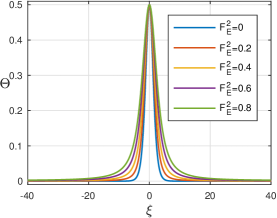
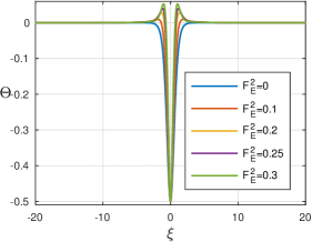
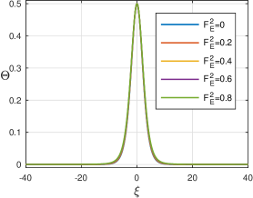
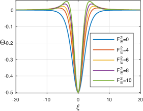
Figure 2: Top: Solitary wave solutions of equation (10) in the absence of vorticity ($\Omega=0$) and different values of $F_{E}$. Parameters: $B=0$ (left) and $B=0.4$ (right). Bottom: Solitary wave solutions of equation (10) with $\Omega=5$ and different values of $F_{E}$. Parameters: $B=0$ (left) and $B=17$ (right).

Typical numerical solitary waves are displayed in Figure 2. We recall that elevation solitary waves occur when $B<B_{c}$ and depression ones when $B>B_{c}$. It is noted that the elevation and depression solitary waves have more ripples appearing on the side of the main pulse when the third-order dispersive term is weak and the electric term in the Hilbert transform is strong, i.e. $\nu$ small and $\gamma$ big in (10). These solutions with decaying oscillatory tails have been previously reported by [20] and [21]. For the purpose of this work, we only focus on the waves shown in Figure 2.

4 Particle trajectories

Particle trajectories beneath the solitary wave (15) can be computed approximately by solving the dynamical system

$$\begin{split}&\frac{dx}{dt}=-\Omega y+\epsilon u(x,y,t)\approx-\Omega y+\epsilon c\Theta(x-(c+\epsilon C)t)),\\ &\frac{dy}{dt}=\epsilon v(x,y,t)\approx-\epsilon c\Theta_{x}(x-(c+\epsilon C)t))(y+1).\\ \end{split}$$ (23)

In order to compute stagnation points, it is convenient to solve equations (23) in the frame that moves with the wave speed, for this purpose we consider the new variables $X=x-(c+\epsilon C)t$ and $Y=y$. In this new reference frame, the streamlines are solutions of the autonomous dynamical system

$$\begin{split}&\frac{dX}{dt}=-\Omega Y+\epsilon c\Theta(X)-(c+\epsilon C),\\ &\frac{dY}{dt}=-\epsilon c\Theta_{X}(X)(Y+1),\\ \end{split}$$ (24)

which can be seen as the level curves of the Hamiltonian $\mathbf{\Psi}(X,Y)$ given by

$$\mathbf{\Psi}(X,Y)=\epsilon c\Theta(X)(Y+1)-\frac{\Omega}{2}Y^{2}-(c+\epsilon C)Y.$$ (25)

Notice that once the solitary wave $\Theta$ is computed numerically through the method proposed in the previous section, the level curves can be easily computed using the function contour that is implemented in MATLAB.

In the absence of surface tension and electric fields, Guan [10] investigated particle trajectories beneath solitary waves in the presence of a linear sheared current through the Korteweg-de Vries equation. He showed that the orbits obtained from the asymptotic approximation agree well with the ones computed through the full Euler equations when the solitary waves have small amplitudes. Based on his results, in all simulations presented in this article, we fix $\epsilon=0.1$.

5 Results and discussion

5.1 Elevation solitary waves

In the absence of an electric field, the increase of the vorticity could cause the appearance of stagnation points (see [22]). It first appears at the bottom and below the crest. As the vorticity increases further, other stagnation points appear in the bulk of the fluid creating a recirculation zone [22]. Therefore, in order to discuss the influence of the electric field in the flow structure beneath solitary waves for $0\leq B<B_{c}$, we first find the smallest value of the vorticity such that a stagnation point appears at the bottom and below the solitary wave crest in the absence of the electric field then follow to study the case where the electric fields are switched on.

The value of the vorticity for which we have a single stagnation point located at the bottom and below the solitary wave crest is obtained by solving for $\Omega$ equation (24) evaluated at $X=0$ and $Y=-1$ which yields the equation

$$0=\Omega+\epsilon cA-(c+\epsilon C).$$ (26)

The solution to equation (26) for $F_{E}=0$ and $B=0$ is $\Omega^{*}\approx 5.2962$ and this value does not vary considerably with $B$ because as pointed out by Flamarion [15] surface tension does not create stagnation points. Moreover, it barely changes the position of the stagnation point below the crest (when it does exist).

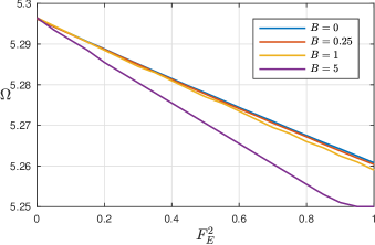
Figure 3: The graph represents the vorticity as a function of the parameter $F_{E}$ in which the first stagnation point gives rise at the bottom of the channel.

Figure 3 displays the solution of equation (26) for different values of the Bond number. These curves correspond to flows with a single stagnation point on the bottom and beneath the crest. Firstly, it is noticed that the solution does not vary much for different values of the Bond number and small values of the parameter $F_{E}$. Besides, we observe that the appearance of the stagnation point on the bottom can occur at a tinnier vorticity with the increase of intensity of the electric field. Secondly, we can regard these curves as bifurcation points that separate the parameter space in two regions according to the number of stagnation points beneath the solitary wave. For those $(F_{E}^{2},\Omega)$ below these curves, there is no stagnation point in the fluid domain. On the other side, for those $(F_{E}^{2},\Omega)$ above these curves, there exist three stagnation points, namely, two saddles at the bottom of the channel and a centre in the bulk of the fluid aligned with the crest of the solitary wave. And there is only one stagnation point at the bottom for those $(F_{E}^{2},\Omega)$ right on the curves. A typical example of this bifurcation is depicted in Figure 4.

We follow to analyse how the strength of the electric field affects the location of the stagnation points. To this end, we fix the vorticity and the surface tension and let $F_{E}$ vary. The left panel of Figure 5 shows the vertical position ($Y^{*}$) of the stagnation point located below the wave crest and the right panel of the same figure presents the horizontal coordinate ($X^{*}$) of the saddle point as a function of the parameter $F_{E}$ for $\Omega=\Omega^{*}$ and $B=0$. Of note, the intensity of $F_{E}$ barely impacts the position of the centre point, however, it does affect the position of the saddle points.

Flamarion et al. [5] showed that the appearance of stagnation points beneath periodic travelling waves can occur at small vorticity with the help of electric fields. Besides, it was shown that the position of all the stagnation points changed significantly with variations in the electric field. The features differ from the discussion presented above for elevation solitary waves where the electric field does not act as a mechanism to help the generation of stagnation points.

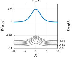
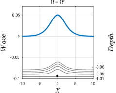
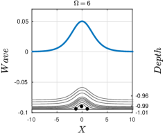
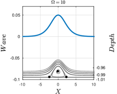
Figure 4: Phase portrait for different values of the vorticity with a solitary wave with amplitude $A=0.5$, $F_{E}^{2}=0.5$ and $B=0$. The critical value of the vorticity in which the first stagnation point appears at the bottom is $\Omega^{*}\approx 5.2780$.

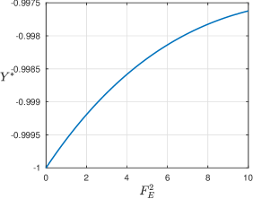
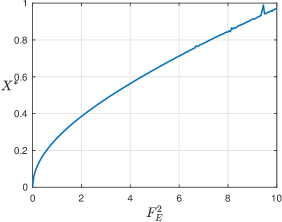
Figure 5: The effect of the electric field in the position of the centre bellow the crest of the solitary wave for $B=0$ and $\Omega=\Omega^{*}$.

5.2 Depression solitary waves

It is known that in the absence of an electric field typical depression solitary wave solutions of equation (10) are $\operatorname{sech}^{2}-$like. For such waves, it is well established that stagnation points never give rise to the bulk of the fluid. As shown by Flamarion [14] stagnation points beneath depression solitary waves can occur only in the presence of decaying or oscillatory tails, which cannot be captured by a third-order KdV equation. As can be seen from Figure 2, under the electrical effect, equation (10) admits depression solitary wave solutions with two elevation dimples on the side of the wave trough. Consequently, an immediate interesting question is whether stagnation points can take place in the bulk of the fluid beneath such depression solitary waves, which will be examined in the rest of the paper.

Other authors have studied the appearance of stagnation points beneath depression solitary waves [14, 15, 23]. However, these works considered gravity-capillary waves in the absence of electric fields. Moreover, it has been shown that the location of the stagnation points does not change much for choices of $B$. Having said this, we focus on investigating the effect of the electric field as a mechanism to create stagnation points. To address this issue we fix the vorticity, the Bond number and vary the intensity of the electric field.

Figure 6 depicts a series of simulations from which we can see that in the presence of a strong electric field stagnation points can appear in the fluid domain. The location of the stagnation points is determined in two ways– (i) by finding the equilibrium points of the dynamical system (24), i.e., we find the zeros of the velocity field or (ii) by the contour function of MATLAB. The flow structure beneath the depression solitary wave can have (i) zero, (ii) two centres (at the bottom), (iii) two centres (in the bulk of the fluid) and four saddles (at the bottom) or (iv) two centres (in the bulk of the fluid) and four saddles (two at the bottom and two in the bulk of the fluid) as stagnation points depending on the intensity of the electric field. This features the bifurcation of flow according to the $F_{E}^{2}$ parameter. Similar descriptions of the arrangement of the stagnation point in the context of gravity-capillary waves were reported in the work of Flamarion [14].

It is well acknowledged that the full Euler equations are the most realistic model to reproduce EHD scenarios in inviscid fluids. However, reduced models can reproduce qualitatively the same features of the flow with comparatively little effort. For instance, our results show that the weakly nonlinear weakly dispersive regime can capture rich flow structures, such as recirculation zones and stagnation points.

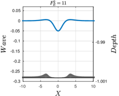
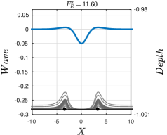
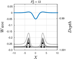
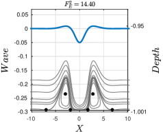
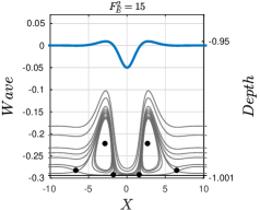
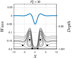
Figure 6: Phase portrait for different values of the vorticity with a solitary wave with amplitude $A=0.5$, $\Omega=5$ and $B=17$. The critical value of the vorticity in which the first stagnation point appears at the bottom is $\Omega^{*}\approx 5.2780$.

6 Conclusion

In the presented study the flow structure beneath EHD flows with constant vorticity was investigated numerically in the Korteweg Benjamin-Ono equation framework. Solitary waves were computed numerically through the standard Newton’s method combined with Fourier spectral methods. This approach allowed us to approximate the velocity field beneath the free surface. As a consequence, the location of stagnation points and details of the recirculation zones formed by them were determined. For elevation solitary waves, we showed that the location of the centre points does not change significantly by variations on the electric field. It is remarkable that for depression solitary waves the electric field acts as a mechanism for the creation of stagnation points. In the absence of an electric field even when the vorticity is strong there is no stagnation point in the bulk of the fluid. The results presented in this work are expected to agree well with the full nonlinear model. An attempt to compare the results predicted by both models is a natural path to be pursued in future.

Data Availability Statement

Data sharing is not applicable to this article as the parameters used in the numerical experiments are informed in this paper.

References

- [1] X. Chen, J. Cheng and X. Yin. Advances and applications of electrohydrodynamics, Chin. Sci. Bull. 48 (2003) 1055–1063.
- [2] D. T. Papageorgiou, Film flows in the presence of electric fields, Ann. Rev. Fluid Mech. 51 (2019) 155–187.
- [3] A. Doak, T. Gao, J.-M. Vanden-Broeck & J. J. S. Kandola, Capillary-gravity waves on the interface of two dielectric fluid layers under normal electric fields, Q. J. Mech. Appl. Math. 73 (2020) 231–250.
- [4] Z. Wang, Modelling nonlinear electrohydrodynamic surface waves over three-dimensional conducting fluids, Proc. R. Soc. A 473 (2017) 20160817.
- [5] M. V. Flamarion, T. Gao, R. Ribeiro-Jr & A. Doak. Flow structure beneath periodic waves with constant vorticity under normal electric fields. Phys. Fluids 34, 127119 (2022).
- [6] H. Gleeson, P. Hammerton, D. Papageorgiou, J.-M. Vanden-Broeck, A new application of the Korteweg-de Vries Benjamin-Ono equation in interfacial electrohydrodynamics, Phys. Fluids 19 (2007) 031703.
- [7] H. Borluk, H. Kalisch, Particle dynamics in the KdV approximation, Wave Motion 49 (2012) 691-709.
- [8] L. Gagnon, Qualitative description of the particle trajectories for n-solitons solution of the korteweg-de Vries equation, Discrete Contin. Dyn. Syst. 37 (2017) 1489-1507.
- [9] Z. Khorsand, Particle trajectories in the Serre equations, Appl. Math. Comput. 230 (2014) 35-42.
- [10] X. Guan, Particle trajectories under interactions between solitary waves and a linear shear current. Theor. App. Mech. Lett. 10 (2020) 125-131.
- [11] A. Alfatih, H. Kalisch, Reconstruction of the pressure in long-wave models with constant vorticity, Eur. J. Mech. B Fluids 37 (2013) 187-194.
- [12] C. Cutis, J. Carter, H. Kalisch, Particle paths in nonlinear Schrödinger models in the presence of linear shear currents, J. Fluid Mech. 855 (2018)
- [13] J. Carter, C. Curtis, H. Kalisch, Particle trajectories in nonlinear Schrd̈inger models, Water Waves 2 (2020) 31-57.
- [14] M.V. Flamarion, Complex flow structures beneath rotational depression solitary waves. Wave Motion. 117, (2023) 103108.
- [15] M.V. Flamarion, Stagnation points beneath rotational solitary waves in gravity-capillary flows. Trends in Computational and Applied Mathematics. (in press) (2023).
- [16] M.V. Flamarion, R. Ribeiro-Jr, Solitary Waves on Flows with an Exponentially Sheared Current and Stagnation Points. Quart. J. Mech. Appl. Math., (2023).
- [17] M. J. Hunt & D. Dutykh, Free Surface Flows in Electrohydrodynamics with a Constant Vorticity Distribution. Water Waves 3, 297–317 (2021).
- [18] G.B. Whitham, Linear and Nonlinear Waves. Wiley. 1974.
- [19] Trefethen LN Spectral Methods in MATLAB. Philadelphia: SIAM; 2001.
- [20] J. P. Albert, J. L. Bona & J. M. Restrepo, Solitary-wave solutions of the Benjamin equation. SIAM J. Appl. Math. 59(6), 2139-2161 (2014).
- [21] V. Dougalis, A. Duran, & D. Mitsotakis, Numerical solution of the Benjamin equation. Wave Motion. 52, 194-215 (2015).
- [22] R. Ribeiro-Jr, P.A. Milewski, A. Nachbin, Flow structure beneath rotational water waves with stagnation points. J. Fluid. Mech. 812 (2017) 792-814.
- [23] Z. Wang, X. Guan & J-M. Vanden-Broeck, Progressive flexural-gravity waves with constant vorticity. J. Fluid. Mech. 995 (2020) A12.