From Ember to Blaze: Swift Interactive Video Adaptation via Meta-Reinforcement Learning

Abstract

Maximizing quality of experience (QoE) for interactive video streaming has been a long-standing challenge, as its delay-sensitive nature makes it more vulnerable to bandwidth fluctuations. While reinforcement learning (RL) has demonstrated great potential, existing works are either limited by fixed models or require enormous data/time for online adaptation, which struggle to fit time-varying and diverse network states. Driven by these practical concerns, we perform large-scale measurements on WeChat for Business’s interactive video service to study real-world network fluctuations. Surprisingly, our analysis shows that, compared to time-varying network metrics, network sequences exhibit noticeable short-term continuity, sufficient for few-shot learning requirement. We thus propose Fiammetta, the first meta-RL-based bitrate adaptation algorithm for interactive video streaming. Building on the short-term continuity, Fiammetta accumulates learning experiences through offline meta-training and enables fast online adaptation to changing network states through few gradient updates. Moreover, Fiammetta innovatively incorporates a probing mechanism for real-time monitoring of network states, and proposes an adaptive meta-testing mechanism for seamless adaptation. We implement Fiammetta on a testbed whose end-to-end network follows the real-world WeChat for Business traces. The results show that Fiammetta outperforms prior algorithms significantly, improving video bitrate by 3.6%-16.2% without increasing stalling rate.

I Introduction

Recent years have witnessed the evolution of video streaming from traditional video on demand (VoD), live TV to ultra-low-latency interactive video applications, such as WeChat, Skype, Zoom, Facetime, etc. Especially with the outbreak of COVID-19 that bounds people with social distancing, the demand for digital classrooms [1], video conferences [2], e-commerce [3], etc. has increased substantially. Polaris Market reports that the global interactive video market is expected to reach a staggering $10.23 billion by 2028 [4].

Despite the fast-paced development, the quality of experience (QoE) of interactive video streaming remains unsatisfactory, such as annoying ultra-blurry images and frequent stalling. The intrinsic reason is that interactive video streaming is highly susceptible to bandwidth fluctuations, due to (i) the strictest latency requirement (e.g., 200 ms) that limits the buffer and resilience to bandwidth fluctuations; (ii) the RTP/UDP protocol that hardly achieves reliable transmission; (iii) the instant capture and encoding that are more likely to waste bandwidth, compared to VoD like bulk data transfer.

To improve the interactive video QoE, extensive research effort has been devoted along bitrate adaptation algorithms. Yet, whether rule-based [5, 6, 7] or learning-based algorithms [8, 9, 10, 11, 12, 13, 14, 15, 16] have their own limitations. (i) Rule-based algorithms [5, 6, 7] commonly adopt universal pre-programmed rules. Much recent literature has shown that these fixed rules can hardly fit diverse and time-varying network states caused by heterogeneous networks (e.g., WiFi, 4G, 5G), complex conditions (e.g., mobility, indoor/outdoor, density), etc. For example, Google Congestion Control (GCC) [5], implemented in WebRTC, encounters overly conservative policies and a lack of agility, which lead to severe bandwidth wastage. (ii) Existing offline-learned neural networks (NNs) [8, 9, 10, 11] are also constrained by their fixed parameters, which fall into the same dilemma as rule-based algorithms. (iii) Existing online learning-based bitrate adaptation algorithms [12, 13, 14, 15, 16] (mainly transfer learning), however, require a large amount of data/time in the face of changing network states, making it difficult to achieve fast adaptation. Moreover, the real-time updates of NNs may converge to local optimum and the trial and error further degrades performance.

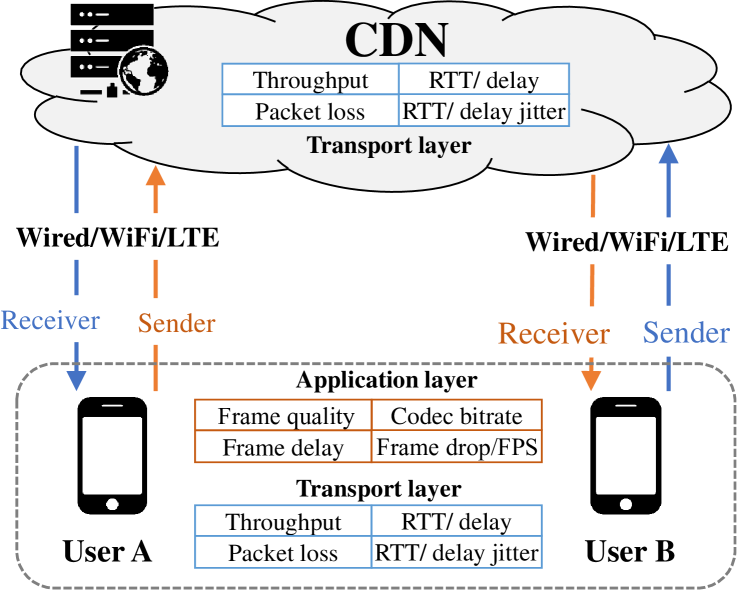
Figure 1: Interactive video system architecture of WeChat for Business.

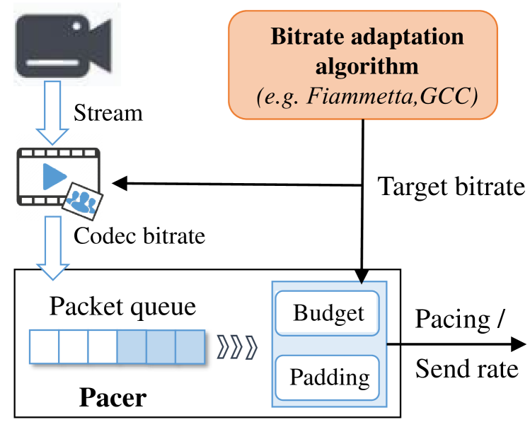
Figure 2: Built-in bitrate control module of interactive video system.

Features	Descriptions
Time span	2022.1.13-15, 2022.5.15-17
Video time	1402382 s
Video sessions	14428
Network types	Wired, WiFi, LTE (4G, 5G)
Countries	Over 200 countries
Volume	7 Gb

TABLE I: Dataset descriptions.

Driven by these practical concerns, we seek to answer a key question: Can interactive video achieve fast adaptation to diverse and time-varying network states, pushing QoE to the limit? To this end, we first conduct large-scale measurements of real-world network fluctuations on WeChat for Business interactive video service. The analysis shows that despite dramatic fluctuations in network metrics, there exists noticeable short-term continuity in network sequences defined by $\{$mean $\mu$, std dev $\sigma$, fluctuation $\omega$, ranges $\boldsymbol{\Delta}\}$, which is sufficient for few-shot learning requirement.

Inspired by the short-term continuity, we propose Fiammetta, the first meta-reinforcement learning (RL)-based bitrate adaptation algorithm for interactive video systems, aiming at maximizing QoE. Fiammetta builds on the merit of “learning to learn” by retaining past learning experiences (i.e., offline meta-training), so as to adapt quickly online with a handful of gradient updates (i.e., meta-testing) to changing network states. Meta-learning is a typical framework for few-sample settings, but Fiammetta is not merely a straightforward environment shift. Instead, it entails three unique challenges.

(i) How to define “tasks” in interactive video streaming? Meta-learning exploits learning experience from previous “tasks” to accelerate online learning. As a matter of course, we consider the adaptation to different “network states” as “tasks”. The problem evolves to how to define “network states” for objectivity of “tasks”, since a mess of network metrics such as loss, RTT, throughput, etc. are deeply affected by bitrate adaptation policies. Once theses metrics are used, the “task” cannot keep constant during policy learning. For this reason, we specifically adopt bandwidth and propagation delay, which characterize environment, traffic flow density, motion state, link length, etc., but marginally affected by bitrate selection. On top of that, we define $\{\mu$, $\sigma$, $\omega\}$ of the bandwidth sequence and set ranges $\boldsymbol{\Delta}$ for a “task” to enhance its continuity.

(ii) How to realize the real-time estimation of “network state” to determine if it is a new “task”? Accurately estimating bandwidth poses challenges, since it cannot be directly measured like RTT, throughput, loss, etc. Rule-based algorithms exploit stable bandwidth probing mechanisms that increase bitrates additively/multiplicatively. Existing RL methods leverage the risky trial and error to probe bandwidth. Meta-RL, however, is more likely to underestimate bandwidth when it increases, as sub-NN is more specialized to one/last “task”, leading to fewer trial-and-error actions. To tackle this problem, we innovatively integrate probing into meta-RL by proposing a bandwidth estimation and filtering mechanism. Specifically, the loss and RTT are used to filter the throughput sequence, which provides hints on network utilization. During the under-use stage, the bandwidth is estimated to be the throughput plus a probing value. This design enables a quick estimation of “network state” and uses the ranges to mitigate the effects of bias.

(iii) How to guarantee seamless adaptation? The time spent on meta-testing might cause a lag in adapting to the changing “network states”, which in turn leads to performance degradation. To handle this issue, we propose an adaptive meta-testing mechanism that sets an activation threshold to $\frac{\boldsymbol{\Delta}}{2}$ of current “network state”, instead of waiting for the detected attributes completely out of ranges $\boldsymbol{\Delta}$. Moreover, we configure proper $\boldsymbol{\Delta}$ to guarantee seamless adaptation according to measurements on WeChat for Business interactive video system.

Results. We implement Fiammetta on a testbed whose end-to-end network follows real-world WeChat for Business traces. We also deploy 3 state-of-the-art solutions: rule-based GCC [5], learning-based OnRL [12], and hybrid Loki [13], using 389 hours of video sessions for a half-month evaluation. Compared with baselines, Fiammetta improves video bitrate by 3.6%-16.2% and cuts stalling rate by 6.3%-21.9%.

Contributions. (i) Through large-scale measurements, we dive into real-world network fluctuations and short-term continuity of network sequences. (ii) We propose Fiammetta, which to our knowledge is the first to deploy meta-RL for fast adaptation to changing network states and maximize QoE. (iii) We implement Fiammetta on a testbed whose end-to-end network follows the real-world WeChat for Business traces, and validate its superiority over state-of-the-art solutions.

The remainder of this paper is organized as follows. §II introduces the measurement study and short-term continuity of network sequences. §III elaborates on the system design. Implementation and evaluation are detailed in §IV and §V. §VI gives a literature review, followed by conclusion in §VII.

II Measurements and Findings

In this section, we conduct a measurement study on WeChat for Business interactive video platform, to investigate the fluctuation characteristics of real-world network states.

II-A Measurement Platform

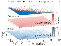
(a) $\hat{B}$ value before and after $\Delta t$.

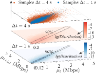
(b) $\mu$ value before and after $\Delta t$.

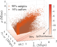
(c) $\sigma$ value before and after $\Delta t$.

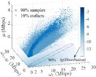
(d) $\omega$ value before and after $\Delta t$.

Figure 3: Real-world network fluctuations.

We log fine-grained end-to-end network metrics and video metrics on WeChat for Business’s interactive video service worldwide. Fig. 2 and Fig. 2 depict the system architecture and the built-in bitrate control module. Integrating transport and application layers, this system applies target bitrates estimated by the bitrate control module to both sending and codec bitrate adaptation. We establish logging points at the CDN and user sides. Therein, only users hold the video encoding and playback functions to execute both sending and codec bitrate adaptation, while the CDN is merely responsible for forwarding and sending bitrate adaptation in the transport layer. Therefore, we log both transport-layer metrics (i.e., throughput, RTT, RTT jitter, packet loss) and application-layer metrics (i.e., FPS, quantization parameter (QP), stalling rate and codec bitrate) at the user side, while only transport-layer metrics of the CDN are recorded.

II-B Dataset Descriptions

Table I summarizes the detailed information of our measurement dataset. Based on WeChat for Business APP, we collect network metrics corresponding to video sessions worldwide during two time spans of Jan 13-15 and May 15-17 with 1 s granularity. The entire dataset consists of 14428 video sessions, with an overall duration of over 1.4 million seconds and a total volume of 7 Gb. These video sessions are built on different heterogeneous networks (e.g., 4G, 5G, WiFi, wired), diverse user devices (e.g., cell phones, tablets, laptops, desktops and even smart watches), covering users in more than 200 countries worldwide. This dataset faithfully logs the real-network network fluctuations worldwide, under the influence of competing traffic, user movements, communication environments, network service providers and frequencies, and has broad coverage in both time and space.

II-C Short-Term Continuity of Network States

Based on the dataset, we qualitatively analyze and quantitatively test the fluctuating characteristics of the network traces.

As mentioned above, the dataset consists of throughput, loss and RTT. However, all these metrics are deeply affected by subjective factors (e.g., bitrate selections), which cannot unambiguously represent background network fluctuations (e.g., competing traffic, user movements). The best is available bandwidth, but it’s hard to measure in real time at fine grain. To handle this issue, we propose a novel bandwidth filtering and estimation mechanism that exploits measurable metrics to estimate bandwidth $\hat{B}$, detailed in §III-B, where we have verified its effectiveness. In what follows, we uses the $\hat{B}$ to investigate the network fluctuating characteristics.

Time-varying characteristic. For a better visualization of network fluctuations, we group all estimated bandwidth pairs, with each pair consisting of estimated $\hat{B}$ before and after a time interval $\Delta t$ within the same video session. Fig. 3(a) plots these pairs with $\Delta t$ of 1 s and 4 s in the form of scatter plots and further depicts their distributions. Specifically, we can notice the high diversity in the back-and-forth $\hat{B}$ fluctuations even at $\Delta t=1$ s. The $\hat{B}$ value exhibits time-varying characteristics that even become more significant as $\Delta t$ increases. When $\Delta t$ reaches 4 s, the fluctuation tends to be more irregular and unpredictable, as the scatter points near the diagonal become less concentrated. In this case, the meta-testing (online adaptation) cannot catch up with the time-varying network fluctuations, when simply using bandwidth value as the definition of the “network state”.

Short-term continuity. We turn to test whether the bandwidth sequence has predictable and regular fluctuating characteristics. Similarly, we depict in Fig. 3(b)-3(d) the mean $\mu$, standard deviation $\sigma$, and fluctuation $\omega$ of the $\hat{B}$ sequences obtained from a sliding window $W_{r}$ before and after a time interval $\Delta t=4$ s (related to the meta-testing time detailed in §III-D). Therein, $\omega$ is the sum of absolute adjacent value differences within $W_{r}$. It is obvious that these sequence properties exhibit more continuity. Even $\Delta t$ reaches 4 s, all the scatter points corresponding to the change in $\mu$, $\sigma$, $\omega$ converge at the diagonal. Furthermore, we find that 90% of the points can be covered by extra adding a small range to $\mu$, $\sigma$, $\omega$. That is to say, if we define the “network state” of a learning task $i$ as a cluster of $\hat{B}$ sequence properties centered at $\{$$\mu_{i}$, $\sigma_{i}$, $\omega_{i}$$\}$ with covering ranges $\boldsymbol{\Delta}_{i}$, the “network state” presents a short-term continuity characteristics.

Since even few-shot learning (i.e., meta-testing process) takes a short period of time, the crux becomes how to define “network state” to gain more continuity and achieve seamless adaptation. A basic rule needs to be satisfied: for most time, the network fluctuations fall within the covering range of “network state” defined for the last “task”. To alleviate the impact of meta-testing lag, the meta-testing process needs to be basically completed before the network changes beyond the range of the last “task”. In short, the meta-testing needs to be faster than the “network state” changes. In this section, we observe the short-term continuity in network sequences, making it a reality to develop meta-RL-based video adaptation algorithm.

III System Design

III-A Overview

Fig. 4 shows the high-level overview of Fiammetta’s design which contains three stages: pre-processing (§III-B), offline meta-training (§III-C) and online meta-testing (§III-D).

• Pre-processing is the basis for subsequent meta-training and meta-testing due to its key steps of trace collection, bandwidth estimation and filtering, and the design and definition of “network state”.

• Meta-training is implemented offline. The end goal is to obtain an initial NN model that can achieve fast adaptation and maximize QoE during meta-testing.

• Meta-testing is performed online to seamless adapt to the changing “network state” based on real-time detection and meta-testing activation mechanism.

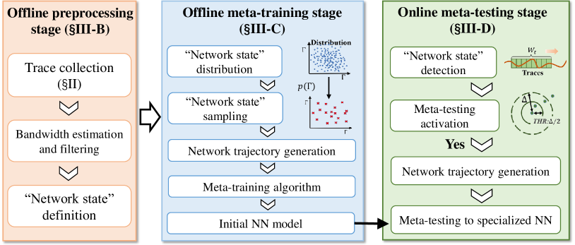
Figure 4: System overview.

III-B Pre-Processing Stage

As shown in Fig. 4, the pre-processing stage prepares for the subsequent meta-training and meta-testing. We focus on the design of bandwidth estimation and filtering mechanism, and the definition of “network state” in this subsection.

Bandwidth estimation and filtering. The definition of “task” for meta-learning tends to be objective, preventing arbitrary “task” changes due to the subjective bitrate selection and policy updates during the training of a given task. The most objective network metrics are available bandwidth and propagation delay, which however cannot be directly measured. Thus, we propose a bandwidth estimation and filtering mechanism based on measurable network metrics. Such mechanism may not be very accurate, but can quickly estimate the trend of “network state” changes and use the defined range to mitigate the impact of bias.

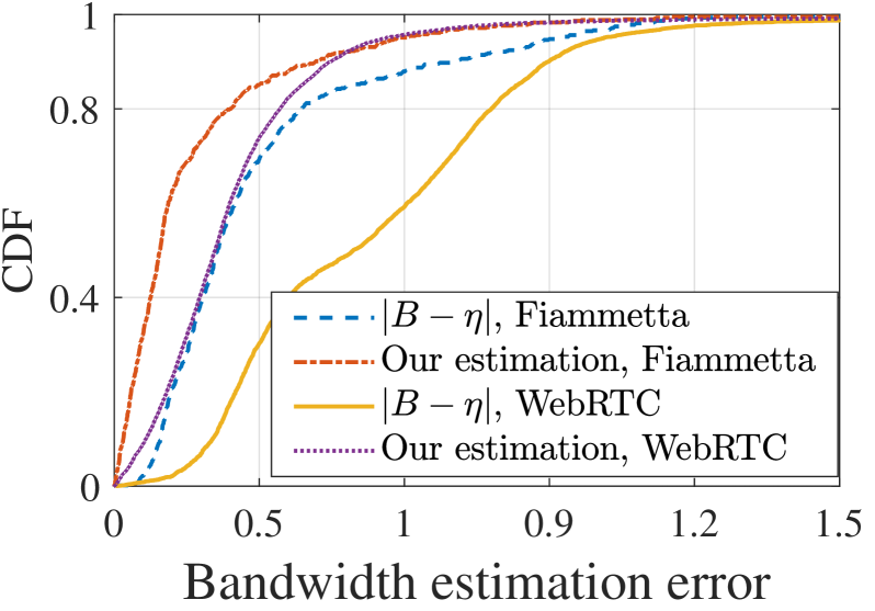
Figure 5: Bandwidth estimation.

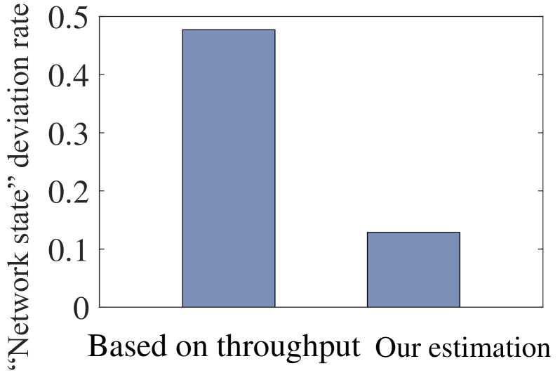
Figure 6: “Network state” estimation.

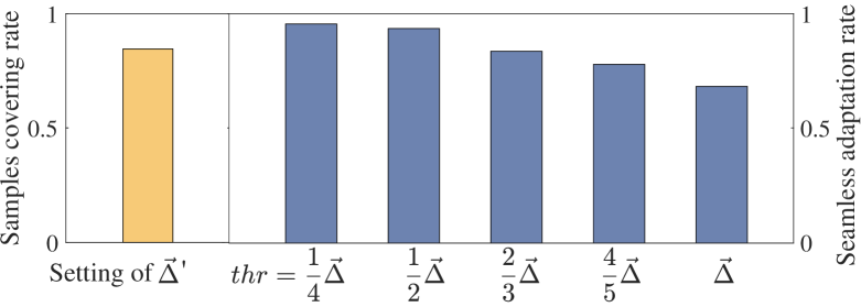
Figure 7: Impact of $\boldsymbol{\Delta}^{\prime}$ and meta-testing $thr$.

A basic principle of the bandwidth estimation is that when there exists packet loss or queuing delay caused by congestion, it is at the stage of full pipe and the throughput $\eta_{t}$ can be regarded as bandwidth [6]. The full pipe is identified (refer to [6]) by the following conditions:

$$F_{t}=(l_{t}>5\%)\;||\;(d_{t}>d_{prop,t}+\sigma(d_{prop})),$$ (1)

$$d_{prop,t}=\min(d_{t^{\prime}},\max(d_{prop}))),$$ (2)

$$t^{\prime}\in[\max(t-W_{d},0),t],$$

where $l_{t}$ denotes the packet loss ratio at time $t$, $d_{t}$ the packet delay, $d_{prop,t}$ the propagation delay, and $F_{t}=1$ indicates the full pipe. Therein, the threshold of 5% (refer to [5, 17]) takes into account the presence of non-congestion packet loss such as lossy wireless links, port flaps on routers, etc., which are not caused by transport-layer bitrate adaptation. The packet delay $d$ is the sum of queuing delay, propagation delay $d_{prop}$ and other smaller values. As path changes on time scales >> $d_{prop}$, the $d_{prop,t}$ can be estimated as a running min over a long time window $W_{d}$ [6]. Once $d_{t}$ exceeds $d_{prop,t}$, we generally assume that there exists queuing delay, i.e., in a full pipe condition. Here, $d_{prop}$ is statistic collected through all $W_{d}$ windows on the dataset (§II-C), and $\sigma(d_{prop})$ is used to tolerate some irregular delay jitters that are not caused by congestion. Furthermore, the $\max(d_{prop})$ is configured to avoid $d_{prop,t}$ overestimation at the beginning of video sessions. Then, we propose to estimate bandwidth $\hat{B}_{t}(Mbps)$ as follows

$$\hat{B}_{t}=\begin{cases}\eta_{t},&F_{t}=1,\\ \max(\eta_{t}+pb^{2}_{t},pb^{1}_{t}),&F_{t}=0.\\ \end{cases}\\$$ (3)

In unfilled conditions, we estimate by a probing mechanism involving both additive and multiplicative increase, based on $\eta_{t}$. Here, $pb^{2}_{t}$ is set to $\Delta_{\mu}$, and $pb^{1}_{t}$ is calculated by

$$pb^{1}_{t}=\begin{cases}\eta_{t}\times(e^{-\eta_{t}-1.3}+1),&F_{t-1}=1,F_{t}=0,\\ pb^{1}_{t-1}\times(e^{-pb^{1}_{t-1}-1.3}+1),&F_{t-1}=F_{t}=0.\end{cases}$$ (4)

Here, $pb^{2}_{t}$ is a constant probing value that does not increase with time to compensate for general phenomenon of $\eta<B$. In contrast, $pb^{1}_{t}$ probes with continual multiplicative increase to fit the bandwidth increment. Besides, when this bandwidth estimation and filtering algorithm is used offline, e.g., in a dataset, we can obtain in advance the later $\hat{B}_{later}$ in full pipe and exploit it to adjust $\hat{B}_{t}$ in unfilled conditions, which is

$$t^{\prime}=\mathop{\arg\max}pb^{1}_{t^{\prime}},\;pb^{1}_{t^{\prime}}<\hat{B}_{later}.$$ (5)

$$\hat{B}_{t}=\begin{cases}\max(pb^{1}_{t^{\prime}}-\eta_{t^{\prime}},pb^{2}_{t})+\eta_{t}\,&t>t^{\prime}\\ \hat{B}_{t},&else.\\ \end{cases}$$ (6)

Fig. 7 and Fig. 7 demonstrate the effectiveness of our estimation, whether the bitrate is controlled by Fiammetta or GCC [5]. Exploiting our measurement testbed (detailed in §IV), we can control the bandwidth trace. Our estimation algorithm is able to significantly reduce the estimation error, compared to the original throughput-to-bandwidth gap. In addition, the impact of these errors can be further mitigated by the range $\boldsymbol{\Delta}$, where the deviation rate of “network state” estimation is reduced from 0.5 to approximate 0.1.

“Network state” definition. We define the “task” as the adaptation to the “network state”, both denoted as $\Gamma_{i},i\in\mathbb{N}^{+}$. Each $\Gamma_{i}$ represents network sequences with similar characteristics, i.e., within a specific property cluster of $\{\mu_{i}$, $\sigma_{i}$, $\omega_{i},d_{prop,i},\boldsymbol{\Delta}_{i}\}$, where $\mu_{i}$, $\sigma_{i}$, $\omega_{i},d_{prop,i}$ are the center and $\boldsymbol{\Delta}_{i}$ the ranges. All these properties are evaluated within the window $W_{r}$ (set as 8 s), with 1 s as the unit time. Wherein, the design of $\boldsymbol{\Delta}$ is critical, as the smaller the $\boldsymbol{\Delta}$, the larger improvement in task-specific updates, but the more likely to be affected by meta-testing lags. We therefore set minimum thresholds $\boldsymbol{\Delta}^{\prime}=\{\Delta^{\prime}_{\mu}=0.2,\Delta^{\prime}_{\sigma}=0.2,\Delta^{\prime}_{\omega}=2\}$ (Mbps) according to §II-C and set $\Delta^{\prime}_{d_{prop}}=3$ ms in the same way. These $\boldsymbol{\Delta}^{\prime}$, on the one hand, cover 90% samples ($\Delta t=4$ s), as shown in Fig. 7, to ensure seamlAess adaptation during meta-testing, and on the other hand, simplify the complexity of $\Gamma$ space to reduce the difficulty of meta-learning.

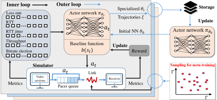
Figure 8: Fiammetta meta-training architecture

III-C Offline Meta-Training

The meta-training is implemented offline. The key steps and the architecture are depicted in Fig. 4 and Fig. 8, respectively.

“Network state” distribution. Among a series of meta-learning algorithms, we choose model-agnostic meta-learning (MAML) [18]. MAML essentially trains initial NN parameters with high sensitivity on a given “task” distribution, allowing for extremely efficient adaptation to “tasks” in few gradient steps. For this reason, we need to obtain the “network state” distribution. Specifically, we first apply the bandwidth estimation algorithm (§III-B) to the dataset collected in §II-C. Then, we utilize the sliding window $W_{r}$ to collect $\{\mu_{t},\sigma_{t},\omega_{t},d_{prop,t},\boldsymbol{\Delta}_{t}\}$ of all network sequences, where $\boldsymbol{\Delta}_{t}=\{\left|\mu_{t}-\mu_{t-\Delta t}\right|,\cdots,\left|d_{prop,t}-d_{prop,t-\Delta t}\right|\}$. We treat each network sequence as the “network state” of $\Gamma_{i}:\{\mu_{i}=\mu_{t},\sigma_{i}=\sigma_{t},\cdots,\boldsymbol{\Delta}_{i}=\max(\boldsymbol{\Delta}_{t},\boldsymbol{\Delta}^{\prime})\}$, without the need for additional categories. It is noteworthy that $\Delta t=4$ s is consistent with that in §III-B and §II-C to maintain the short-continuity of “network states”. Finally, based on the multidimensional “network states”, we calculate their joint probability densities on the basis of fine-grained partitioning, and then combine interpolation to obtain the probability density function $p(\Gamma)=p(\mu,\sigma,\omega,\boldsymbol{\Delta})\times p(d_{prop})$.

“Network state” sampling. Based on $p(\Gamma)$, we sample “network state” $\Gamma_{i},i\in\mathbb{N}^{+}$ to provide tasks for meta-training process, depicted in Fig. 8. Theoretically, the more tasks sampled during meta-training process, the smaller the difference between the distribution of the sampled tasks and $p(\Gamma)$, and the more robust the performance is over $p(\Gamma)$.

Generation of network trajectories. For each task, sufficient network trajectories are necessary as training samples. However, some “network states” $\Gamma$ with small probabilities often encounter the problem of insufficient collected network trajectories during meta-training. Besides, there is also not enough time to obtain network trajectories of new “network states” during meta-testing. Therefore, we explore a second approach which involved generating synthetic network trajectories, in addition to collecting real trajectories.

Given a $\Gamma_{i}$, we first sample $\mu$, $\sigma$, $d_{prop}$ in their respective ranges, following Gaussian distribution to guarantee that the sampling probability at the center is slightly larger. Similarly, we sample $d_{prop}$ in the same way. The purpose of this is to provide optimization preference for each $\Gamma_{i}$. Then, we generate bandwidth samples through two distributions. One is the Gaussian distribution, commonly used in studies [8, 19] for synthetic trajectory generation, and the other is the beta distribution that is built on a range $\left[0,max\right]$ and can easily achieve asymmetric sampling. Here, $max$ is the maximum $\hat{B}$ in the dataset. For any given $\mu$ and $\sigma$, if $\left[\mu-3\sigma,\mu+3\sigma\right]\subseteq\left[0,max\right]$ (3$\sigma$ rule [20]), we assume a Gaussian distribution for bandwidth samples, otherwise, the beta distribution is adopted as an alternative. Finally, we repeat the first two steps to obtain enough bandwidth samples, and then arrange them into trajectories in different orders, among which the trajectories that do not satisfy $\Delta_{\mu_{i}},\Delta_{\sigma_{i}},\Delta_{\omega_{i}}$ are filtered out.

Meta-training for initial NN model. Fig. 8 depicts the Fiammetta meta-training architecture. We proceed to describe the customized designs and key algorithms involved.

(i) State and Action. At any time $t$, the RL agent takes the state $s_{t}$ as input, the neural network as a function $\pi_{\theta_{t}}$, and outputs a target bitrate $a_{t}$ to interact with the interactive video system. The end goal is to find the optimal bitrate adaptation policy, i.e., $\pi^{*}_{\theta}:s_{t}\rightarrow a_{t}$ to maximize QoE. Specifically, $s_{t}$ is denoted as $\{\boldsymbol{\eta}_{t},\boldsymbol{b}_{t-\Delta t^{\prime}},\boldsymbol{l}_{t},\boldsymbol{d}_{t},\boldsymbol{j}_{t}\}$, representing sequences of throughput, target bitrate, packet loss ratio, delay, and delay jitter over past 3 s with $\Delta t^{\prime}=0.1$ s as the unite time. All these metrics can be obtained at the sender via periodic RTCP feedback. After observing $s_{t}$, the RL agent outputs $a_{t}$, chosen from 21 discrete actions set $\{-2,-1.8,\cdots,1.8,2\}$. Here, $a_{t}$ represents the scaling factor between two consecutive target bitrate selection, i.e., $b_{t}=b_{t-\Delta t^{\prime}}\times e^{a_{t}}$, like Libra [21].

(ii) Reward. Upon determining $a_{t}$, Fiammetta interacts with the interactive video system by adjusting both codec bitrate and sending rate, and then gets a reward $r_{t}$ to update $\pi_{\theta}$. We exploit QoE as the criterion for designing $r_{t}$, which is

$$r_{t}=w_{1}\times\eta_{t}-w_{2}\times l_{t}-w_{3}\times d_{t}-w_{4}\times\left|b_{t}-b_{t-\Delta t^{\prime}}\right|.$$ (7)

Therein, all these metrics are averaged over one unit time, i.e., from $t-\Delta t^{\prime}$ to $t$. $\left|b_{t}-b_{t-\Delta t^{\prime}}\right|$ enforces the codec bitrate smoothness to prevent large frame delay jitter and quality jitter. Referring to recent studies [12, 13], we empirically set these four weights to 50, 50, 200 and 20, respectively.

(iii) NN structure. For a start, state sequences are flattened before being fed into networks. The actor network consists of three fully connected layers with 128, 64 and 32 neurons respectively, followed by an activation function. The baseline function $b^{\pi_{\theta}}(s)$ simply implements a linear fit as an average expected reward of $s$ under $\pi_{\theta}$.

(iv) Training algorithm. The entire meta-training consists of two parts: inner loop and outer loop. The inner loop is responsible for task-specific optimization, and the outer loop is to obtain an efficient initial NN model, which enables fast adaptation in the inner loop.

During the inner loop, each $\Gamma_{i}$ contains an initial state distribution $p_{i}(s_{t})$ and a transition distribution $p_{i}(s_{t+\Delta t^{\prime}}|s_{t},a_{t})$. $\Gamma_{i}$ is therefore a Markov decision process (MDP). During each gradient update, the RL agent is allowed to query $K$ trajectories $\xi_{k}=\{s_{\Delta t^{\prime}},a_{\Delta t^{\prime}},r_{\Delta t^{\prime}},\cdots,s_{N},a_{N},r_{N}\}\;(k=1,\cdots,K)$, which are sampled through rollouts by $\pi_{\theta_{i}}$ (initially set as $\theta_{0}$) on network trajectories (detailed above) and simulators (§IV). Then, the cumulative reward $R^{\pi_{\theta_{i}}}(s_{t},a_{t})=\sum_{t^{\prime}=\frac{t}{\Delta t^{\prime}}}^{\frac{t+3}{\Delta t^{\prime}}}\gamma^{(t^{\prime}-\frac{t}{\Delta t^{\prime}})}r_{t^{\prime}\times\Delta t^{\prime}}$ is used to update $\theta_{i}$ as follows

$$\mathcal{L}_{\Gamma_{i}}(\theta_{i}) =\mathbb{E}_{\xi_{k}\sim(\pi_{\theta_{i}},p_{i})}\left[\sum_{t}^{\xi_{k}}\hat{A}^{\pi_{\theta_{i}}}(s_{t},a_{t})\right],$$ (8)

$$\theta_{i} \leftarrow\theta_{i}+\alpha\Delta_{\theta_{i}}\mathcal{L}_{\Gamma_{i}}(\theta_{i}),$$ (9)

where $\mathcal{L}$ is the loss function, $\alpha$ the learning rate, $b^{\pi_{\theta_{i}}}(s_{t})$ the average expected reward at $s_{t}$ under $\pi_{\theta_{i}}$, $\hat{A}^{\pi_{\theta_{i}}}(s_{t},a_{t})=R^{\pi_{\theta_{i}}}(s_{t},a_{t})-b^{\pi_{\theta_{i}}}(s_{t})$ the advantage function, representing the extra benefit from a certain $a_{t}$. Besides, “3 s” is the empirically configured time that Fiammetta considers for the future. When adapting to $\Gamma_{i}$, the NN parameters evolve from $\theta_{0}$ to $\theta_{i}$ according to Eq. (9) through only 3 gradient updates that are sufficient for convergence.

The outer loop further improves the performance of $\pi_{\theta_{i}}$ by updating initial $\theta_{0}$ following PPO algorithm [22]. During each round of outer loop, Fiammetta samples $M$ tasks from $p(\Gamma)$, updates to corresponding $\{\theta_{i}\}_{i=1}^{M}$ in the inner loop, and evaluates by resampling $K$ trajectories $\{\xi_{k,i}\}_{k=1}^{K}$ on each task using $\pi_{\theta_{i}}$. Then, Fiammetta obtains the loss function $\mathcal{L}$ and updates $\theta_{0}$ by

$$\mathcal{L}^{\theta^{\prime}_{0}}(\theta_{0})= \mathbb{E}^{i\sim p(\Gamma)}_{\xi_{k,i}\sim(\pi_{\theta_{i}},p_{i})}\bigg{[}\sum_{t}^{\xi_{k,i}}\min\left(\delta^{\theta^{\prime}_{0}}(\theta_{0})\hat{A}^{\pi_{\theta_{i}}}(s_{t},a_{t}),\right.$$

$$\left.clip(\delta^{\theta^{\prime}_{0}}(\theta_{0}),1-\epsilon,1+\epsilon)\hat{A}^{\pi_{\theta_{i}}}(s_{t},a_{t})\right)\bigg{]},$$ (10)

$$\theta_{0}\leftarrow \theta_{0}+\beta\Delta_{\theta_{0}}\mathcal{L}^{\theta^{\prime}_{0}}(\theta_{0}),$$ (11)

where $\theta^{\prime}_{0}$ is the old initial parameters before each round of outer-loop update, and $\delta^{\theta^{\prime}_{0}}(\theta_{0})=\frac{\pi_{\theta_{0}}(s_{t},a_{t})}{\pi_{\theta_{old,0}}(s_{t},a_{t})}$ represents the ratio of a new policy and its old one. The basic idea is to make the update of $\theta_{0}$ smoother and avoid gradient oscillations by clipping $\delta^{\theta^{\prime}_{0}}(\theta_{0})$ values that are out of $[1-\epsilon,1+\epsilon]$.

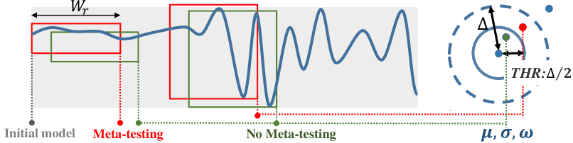
Figure 9: Fiammetta meta-testing design.

III-D Online Meta-Testing

Based on the initial NN model, Fiammetta achieves seamless adaptation to time-varying “network states” through online meta-testing, the steps of which are shown in Fig. 4 and Fig. 9.

“Network state” monitoring. Fiammetta monitors the real-time “network state” by computing $\mu_{t},\sigma_{t},\omega_{t}$ and $d_{prop,t}$ of the network sequence within a sliding window $W_{r}$ over past $8$ s. It is noteworthy that the bandwidth $\hat{B}$ and $d_{prop}$ are estimated following the steps in §III-B, and the sliding window is moved at a granularity of 1 s for real-time assurance.

Meta-testing activation. The target of meta-testing activation is to achieve a seamless adaptation between “network state” changes. Therefore, it cannot wait until the detected attributes, such as $\mu_{t},\sigma_{t},\omega_{t},d_{prop,t}$ are out of the ranges $\boldsymbol{\Delta}_{last}$ of last “task”. As an alternative, we set the activation threshold to $\frac{\boldsymbol{\Delta}_{last}}{2}$ according to Fig. 7, i.e., each of $\left|\mu_{t}-\mu_{last}\right|>\frac{\Delta_{\mu,last}}{2}$, $\left|\gamma_{t}-\gamma_{last}\right|>\frac{\Delta_{\gamma,last}}{2}$, $\cdots$ will activate meta-testing. Then, the seamless adaptation is ensured by alleviating the effect of meta-testing lag, shown in Fig. 9. Note that $\boldsymbol{\Delta}$ is also required to be compliant with this lag. As meta-testing (i.e., inner loop with 3 gradient updates) takes roughly 2 s according to our statistics, $\boldsymbol{\Delta}$ needs to cover at least 4 s of network variations, which is the reason for configuring $\Delta t=4$ s (§II-C) and obtaining $\boldsymbol{\Delta}^{\prime}$ (§III-C) based on this.

Meta-testing. Consistent with the inner loop, meta-testing is responsible for adapting to varying "network states" detected in real time. Upon activation, the new “network state” $\Gamma_{i}:\{\mu_{i}=\mu_{t},\sigma_{i}=\sigma_{t},\omega_{i}=\omega_{t},\boldsymbol{\Delta}_{i}=\max(\boldsymbol{\Delta}_{t},\boldsymbol{\Delta}^{\prime})\}$ is generated, where $\boldsymbol{\Delta}_{t}=\{\left|\mu_{t}-\mu_{last}\right|,\left|\sigma_{t}-\sigma_{last}\right|,\left|\omega_{t}-\omega_{last}\right|\}$. Then, we follow the workflow of inner loop by first sampling $K$ trajectories of $\Gamma_{i}$, again obtained through $K$ rollouts on synthetic network trajectories (§III-C) and simulators (§IV). Then, the specialized NN parameters $\theta_{i}$ for $\Gamma_{i}$ can be obtained through 3 gradient updates based on Eq. (8)-(9).

IV Implementation

Testbed implementation. We build an end-to-end measurement testbed and exploit the real-world network traces (detailed in §II) sponsored by WeChat for Business APP to test the performance of Fiammetta and baseline algorithms. As shown in Fig. 10, the testbed mainly consists of two PCs running WebRTC as a video traffic transceiver pair and one PC controlling network link through the TC (traffic control) tool [23]. Besides, we implement Fiammetta and learning-based baseline algorithms on a remote RL server, and the video transceiver pair is connected to the RL server via an additional router to query the target bitrate. The RL server is a desktop equipped with Intel Core i7-9700K CPU, Geforce RTX 1080Ti GPU, 32-GB memory and Ubuntu 18.04. We implement Fiammetta with PyTorch version 1.10.2.

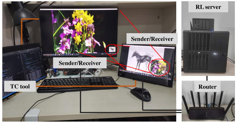
Figure 10: Testbed setup.

Fig. 11 further shows the detailed system implementation of Fiammetta, which works by replacing the bitrate control module in interactive video system. At run time, the sender offloads network metrics (obtained from RTCP feedback) to the RL server in real-time and adopt the bitrate decision $a_{t}$ selected by the RL model $\pi_{\theta_{i}}$. Moreover, we detach meta-testing from the front-end query service to ensure responsiveness. Specifically, we set up a back-end process to receive the transition tuples from the front-end and conduct meta-testing without disturbing it. Once meta-testing is completed, the old NN parameters $\theta_{old}$ in the front-end will be replaced by the new parameters $\theta_{new}$. To further reduce computation overhead, we dynamically store partial specialized NN parameters $\theta_{i}$ on the server according to the access frequency, in addition to initial NN parameters.

Simulator. Our simulator consists of two modules: (i) A video compression module that compresses real video to different bitrates of $\{0.1,0.2,\cdots,2.5\}$ Mbps, and records each frame size to faithfully simulate frame size jitters. At run time, this module continuously outputs frame sizes of the video that has the closest bitrate to the target. (ii) A transport module that packages frame-sized random data into RTP packets and faithfully simulates the pacer mechanism to send packets into a simulated network path. The bandwidth and propagation delay are configured according to the WeChat for Business traces for Fiammetta training.

V Evaluation

V-A Methodology

Trace-driven testbed experiments. We train and test Fiammetta & baseline algorithms on the same datast (detailed in §II) with 75% the training set and 25% the test set. As the network bandwidth is hard to accurately measure at fine grain, we use throughput as bandwidth for experiments. This certainly simplifies the experiment by getting a precise “network states” distribution $p(\Gamma)$. However, we want to make it clear that our design can handle real-world deployments without explicit bandwidth information.

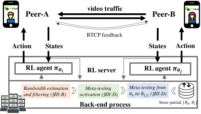
Figure 11: System implementation of Fiammetta.

TABLE II: Overall performance regarding application and transport-layer metrics ($Mean\pm Std\,Dev$)

Algorithms	Application-layer metrics					Transport-layer metrics				QoE/ Reward
	FPS	PSNR (dB)	Stalling rate (FPS <12, %)	Frame delay (ms)	Frame delay jitter (ms)	RTT (ms)	Loss rate (%)	Throughput (Mbps)	Bitrate jitter (Mbps/10min)
GCC [5]	$29.41\pm 4.41$	$33.17\pm 7.98$	$0.83\pm 5.27$	$\boldsymbol{160.23}\pm\boldsymbol{45.42}$	$\boldsymbol{5.25}\pm\boldsymbol{10.35}$	$68.93\pm 110.27$	$1.68\pm 1.01$	$0.74\pm 0.23$	$1.09\pm 2.04$	22.85
OnRL [12]	$29.02\pm 4.29$	$34.12\pm 7.32$	$0.96\pm 3.55$	$170.68\pm 36.32$	$5.53\pm 10.82$	$73.95\pm 119.01$	$2.00\pm 1.33$	$0.83\pm 0.25$	$\boldsymbol{0.92}\pm\boldsymbol{5.20}$	26.05
Loki [13]	$29.04\pm 4.36$	$33.82\pm 6.55$	$0.80\pm 2.32$	$165.21\pm 38.34$	$5.343\pm 10.92$	$69.29\pm 97.86$	$1.88\pm 1.25$	$0.78\pm 0.22$	$1.20\pm 1.81$	24.74
Fiammetta	$\boldsymbol{29.51}\pm\boldsymbol{3.41}$	$\boldsymbol{34.51}\pm\textbf{7.27}$	$\boldsymbol{0.75}\pm\boldsymbol{2.31}$	$162.53\pm 30.24$	$5.27\pm 9.63$	$\boldsymbol{68.51}\pm\boldsymbol{63.86}$	$\boldsymbol{1.65}\pm\boldsymbol{1.25}$	$\boldsymbol{0.86}\pm\boldsymbol{0.24}$	$1.09\pm 2.16$	$\boldsymbol{28.94}$

Baseline algorithms are listed in the following

• GCC [5], as an official congestion control algorithm, is widely used in mainstream interactive video systems, such as WeChat, Google Hangouts, etc. The core idea is to adopt a combination of loss-based and delay-gradient-based methods to avoid congestion and adjust bitrates.

• OnRL [12] is the first online-RL-based adaptation algorithm for interactive video systems. We train it with the same training set directly on our testbed, spending about 12 days with 291 hours, and implement online adaptation during the 4-day-long test period of 100 hours.

• Loki [13] proposes to fuse the rule-based GCC with the RL-based algorithm at the feature level to improve the long-tail performance. Following Loki, we “blackboxify” GCC, integrate it with OnRL, and then retrain the new NN on our testbed with the same training set. The online adaptation is also performed during testing process.

V-B Comparison with Baseline Algorithms

The comparison results are summarized in Table II.

Application-layer metrics. Fiammetta significantly outperforms all three competing algorithm: (i) Compared to GCC, Fiammetta improves PSNR by 1.34 dB and decreases stalling rate by $9.6\%$. More importantly, Fiammetta is also comparable to the conservative GCC in terms of FPS, frame delay and jitters. (ii) In comparison to learning-based OnRL and Loki, Fiammetta cuts stalling rate by 21.9% and 6.3%, respectively, and is also better in frame quality, with a little improvements in both PSNR and FPS. Also, the frame delay and delay jitter of Fiammetta exhibit better performance than Loki, OnRL.

Transport-layer metrics. Similarly, Fiammetta achieves remarkable gains in most transport-layer metrics: (i) Consistent with application-layer metrics, Fiammetta effectively improves throughput by 3.6%, 10.3%, 16.2% over OnRL, Loki and GCC, respectively. (ii) Meanwhile, the RTT of Fiammetta significantly drops by 1.1%, 7.4%, synchronized with loss rate reduction of 12.3%, 17.5%, compared to Loki and OnRL. These metrics are at the same level as the conservative GCC. (iii) While the bitrate jitter of Fiammetta is slight worse than OnRL, it performs comparable to GCC and better than Loki.

QoE/Reward. Table II further demonstrates the QoE/reward to provide an overall evaluation. For fairness comparison, all RL-based algorithms are trained using the same QoE/Reward setting defined in §III-C. We can notice that Fiammetta outperforms OnRL by 11.1% in QoE, and the gap gradually increases to 17.0% and 26.7% when compared to Loki and GCC, respectively. These results validate the overall superiority of Fiammetta, by achieving a better dynamic balance between conflicting metrics such as delay, packet loss, smoothness and throughput to maximize interactive video QoE.

Figure 12: A microscopic showcase of a 600-second session.

A microscopic showcase. We find that Fiammetta’s gains stem from its ability to quickly generate and switch to strategies that fit the current “network state”. Fig. 12 exhibits a representative 600-second session. (i) When the bandwidth is relatively stable, Fiammetta follows closely, maximizing bandwidth utilization with minimum magnitude of probing. The reason is that Fiammetta can always have rough priori assumptions about “network states”. At run time, when the “network state” is roughly detected, Fiammetta can quickly generate strategies that fit the range of “network state”, eliminating many substantial trial-and-error behaviors. In comparison, GCC suffers from periodic bitrate degradation due to its AIMD-based probing mechanism, while OnRL exhibits frequent overshoots. Affected by the integration with GCC, Loki also encounters unnecessary bitrate drops, when GCC bitrate goes down and occupies much larger impacting factor, resulting in a loss of bandwidth utilization. (ii) When the bandwidth fluctuates dramatically (280-370 s), Fiammetta can also benefit from the priori assumptions and generate relatively conservative strategies compared to OnRL, yielding an RTT comparable to GCC and with higher throughput.

Figure 13: Fiammetta’s adaptability to different “network states”, compared to baseline algorithms.

V-C Comparison across Different “Network States”

We further evaluate Fiammetta across large/small stable/dynamic bandwidth, with results depicted in Fig. 13.

Large stable bandwidth. We first evaluate Fiammetta in the highest-quality “network state” with large stable bandwidth ($\mu\in[1,3]$ and $\sigma\in[0,0.1]$). Fiammetta achieves noticeable video clarity improvements, boosting throughput by 9.5%-21.4%, and PSNR by 0.2 dB-2.6 dB across three baseline algorithms. Meanwhile, Fiammetta also achieves better performance in RTT and stalling rates. This results further validate that priori rough assumptions about “network states” help Fiammetta to achieve better performance.

Large dynamic bandwidth. For the “network state” with large but dynamic bandwidth ($\mu\in[1,3]$ and $\sigma\in[0.3,0.5]$), Fiammetta still achieves throughput gains by 2.2%-10.3%, and PSNR gains by 0.2 dB-1.9 dB. Meanwhile, both RTT and stalling rate exhibit noticeable reductions compared to baseline algorithms This shows that Fiammetta can quickly switch to a relatively conservative strategy when bandwidth fluctuates, to avoid much latency increase.

Small stable bandwidth. When adapting to “network state” with small stable bandwidth ($\mu\in[0.5,1]$ and $\sigma\in[0,0.1]$), Fiammetta achieves stalling rate comparable to GCC and significantly better than Loki and OnRL. Moreover, Fiammetta’s PSNR and throughput are in between OnRL and Loki, achieving global optimum in QoE. Such results suggest Fiammetta has essentially developed strategies for small stable bandwidth, instead of blindly probing, causing frequent overshoots.

Small dynamic bandwidth. The small dynamic bandwidth ($\mu\in[0.5,1]$ and $\sigma\in[0.3,0.5]$) is considered by us as the worst “network state”, but Fiammetta still achieves promising results in this case. Instead of blindly seeking to fit the bandwidth fluctuation curve, Fiammetta adopts a relatively conservative strategy. It achieves 7.5%-19.8% throughput gains, and hence 0.4 dB-2.8 dB PSNR gains, with reductions in stalling rate of 8.3%-20.6% over three baseline algorithms.

V-D Comparison of Fiammetta w/ and w/o Meta-Testing

In this subsection, we proceed to investigate whether the gains of Fiammetta are due to the fast adaptation of online meta-testing to changing “network states” or to the superiority of the initial NN itself. We conduct experiments to compare the performance of Fiammetta w/ and w/o meta-testing. Through the results in Fig. 14, we note that Fiammetta w/ meta-testing achieves performance gains across all application- and transport-layer metrics: (i) For the application-layer metrics, the most significant improvements come from the 7.5% increase in PSNR and the 19.5% reduction in stalling rate. (ii) For the transport-layer metrics, the throughput is improved by 9.7%, with reductions in RTT and bitrate jitter of 7.8% and 60.8%, respectively, compared to Fiammetta w/o meta-testing.

VI Related Work

Interactive video adaptation. Much effort has gone into developing bitrate adaptation algorithms for interactive video streaming, which falls into two categories: (i) rule-based algorithms [5, 6, 7], and (ii) learning-based algorithms [11, 12, 13, 14, 15]. Rule-based algorithms [5, 6, 7] typically follow AIMD-like approaches for bitrate adaptation, based on loss, delay and delay jitter, etc. However, such pre-programmed universal rules can hardly fit diverse and heterogeneous modern networks. The learning-based algorithms consist of offline [11] and online learning approaches [12, 13, 14, 15]. For instance, Concerto [11] adopts imitation learning offline. OnRL [12] is the first to achieve fully online learning in interactive video applications via federated learning. Loki [13] proposes tight coupling between RL and GCC. Notwithstanding, the offline-trained model still suffers from fixed parameters. These online-learning algorithms [12, 13, 14, 15], however, rely on a large amount of data/time, which hinders fast adaptation to changing “network states”. Besides, Salsify [24] designs customized codec to address the mismatch between the actual codec bitrate and transport/target bitrate. In addition, many parallel studies [8, 9, 10, 16, 19] target bitrate adaptation in VoD streaming, which also provide much inspiration for Fiammetta.

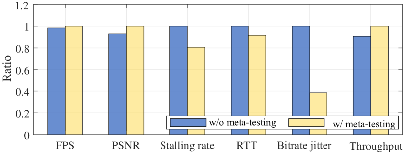
Figure 14: Comparison of Fiammetta w/ and w/o meta-testing.

Meta-reinforcement learning. Meta-learning [25] is a typical framework for addressing challenging few-shot learning setting by providing reasonable assumptions : (i) a task distribution $p(\Gamma)$ exists, (ii) the target new task obeys $p(\Gamma)$; (iii) a meta-training set sampled from $p(\Gamma)$ can be obtained to train the model, and (iv) another meta-testing set sampled from $p(\Gamma)$ can be used to evaluate the expected performance [25]. Fiammetta basically follows these assumptions. The research on meta-RL includes meta-learning initial NN parameters [18, 26], loss functions [27], adaptation process [28], which are all key components of RL. Among them, MAML [18] is a landmark work that adjusts simply initial NN parameters, which is sample efficient, lightweight and extremely suitable for few-shot learning settings. In addition, Fiammetta is highly compatible with MAML constraints such as fixed NN structure (e.g., input/output sizes) and strong correlation among tasks.

VII Conclusion

Fiammetta represents the first meta-RL-based bitrate adaptation algorithm for interactive video system. It marks a new optimization modality that fast adaptation to changing network states becomes a reality by few-shot learning. This system is inspired by an observation that network sequences exhibit noticeable short-term continuity sufficient for few-shot learning, drawn from a real-world measurement study on WeChat for Business interactive video system. We evaluate Fiammetta on a local testbed with network links following WeChat for Business traces. Experimental results confirm the superiority of Fiammetta compared to state-of-the-art algorithms.

References

- [1] Matthew Lynch. The impact of interactive videos in the classroom. https://www.thetechedvocate.org/the-impact-of-interactive-videos-in-the-classroom/. Online; accessed Sep 23, 2020.
- [2] Justin Pot. The best video conferencing software for teams in 2022. https://zapier.com/blog/best-video-conferencing-apps/. Online; accessed May 11, 2022.
- [3] Zanna Zhang. How interactive e-commerce in china drives the next phase of e-commerce. https://pandaily.com/. Online; accessed Aug 13, 2020.
- [4] Allan Parker. New study: Latest insights on interactive video wall market share to 10% CAGR by 2028. https://whatech.com/og/markets-research/semiconductor-and-electronics/. Online; accessed Jan 9, 2022.
- [5] Gaetano Carlucci, Luca De Cicco, Stefan Holmer, and Saverio Mascolo. Analysis and design of the google congestion control for web real-time communication (WebRTC). In Proceedings of the 7th International Conference on Multimedia Systems, pages 1–12, 2016.
- [6] Neal Cardwell, Yuchung Cheng, C Stephen Gunn, Soheil Hassas Yeganeh, and Van Jacobson. BBR: congestion-based congestion control. Communications of the ACM, 60(2):58–66, 2017.
- [7] Subir Varma. Internet congestion control. Morgan Kaufmann, 2015.
- [8] Hongzi Mao, Ravi Netravali, and Mohammad Alizadeh. Neural adaptive video streaming with pensieve. In Proceedings of the conference of the ACM special interest group on data communication, pages 197–210, 2017.
- [9] Xutong Zuo, Jiayu Yang, Mowei Wang, and Yong Cui. Adaptive bitrate with user-level QoE preference for video streaming. In IEEE INFOCOM 2022-IEEE Conference on Computer Communications, pages 1279–1288, 2022.
- [10] Francis Y Yan, Hudson Ayers, Chenzhi Zhu, Sadjad Fouladi, James Hong, Keyi Zhang, Philip Levis, and Keith Winstein. Learning in situ: a randomized experiment in video streaming. In 17th USENIX Symposium on Networked Systems Design and Implementation (NSDI 20), pages 495–511, 2020.
- [11] Anfu Zhou, Huanhuan Zhang, Guangyuan Su, Leilei Wu, Ruoxuan Ma, Zhen Meng, Xinyu Zhang, Xiufeng Xie, Huadong Ma, and Xiaojiang Chen. Learning to coordinate video codec with transport protocol for mobile video telephony. In The 25th Annual International Conference on Mobile Computing and Networking, pages 1–16, 2019.
- [12] Huanhuan Zhang, Anfu Zhou, Jiamin Lu, Ruoxuan Ma, Yuhan Hu, Cong Li, Xinyu Zhang, Huadong Ma, and Xiaojiang Chen. OnRL: improving mobile video telephony via online reinforcement learning. In Proceedings of the 26th Annual International Conference on Mobile Computing and Networking, pages 1–14, 2020.
- [13] Huanhuan Zhang, Anfu Zhou, Yuhan Hu, Chaoyue Li, Guangping Wang, Xinyu Zhang, Huadong Ma, Leilei Wu, Aiyun Chen, and Changhui Wu. Loki: improving long tail performance of learning-based real-time video adaptation by fusing rule-based models. In Proceedings of the 27th Annual International Conference on Mobile Computing and Networking, pages 775–788, 2021.
- [14] Lei Zhang, Yong Cui, Mowei Wang, Kewei Zhu, Yibo Zhu, and Yong Jiang. DeepCC: Bridging the gap between congestion control and applications via multi-objective optimization. IEEE/ACM Transactions on Networking, 2022.
- [15] Yiqing Ma, Han Tian, Xudong Liao, Junxue Zhang, Weiyan Wang, Kai Chen, and Xin Jin. Multi-objective congestion control. In Proceedings of the Seventeenth European Conference on Computer Systems, pages 218–235, 2022.
- [16] Tianchi Huang, Chao Zhou, Xin Yao, Rui-Xiao Zhang, Chenglei Wu, Bing Yu, and Lifeng Sun. Quality-aware neural adaptive video streaming with lifelong imitation learning. IEEE Journal on Selected Areas in Communications, 38(10):2324–2342, 2020.
- [17] Mo Dong, Tong Meng, Doron Zarchy, Engin Arslan, Yossi Gilad, Brighten Godfrey, and Michael Schapira. Pcc vivace:online-learning congestion control. In 15th USENIX Symposium on Networked Systems Design and Implementation (NSDI 18), pages 343–356, 2018.
- [18] Chelsea Finn, Pieter Abbeel, and Sergey Levine. Model-agnostic meta-learning for fast adaptation of deep networks. In International conference on machine learning, pages 1126–1135, 2017.
- [19] Zahaib Akhtar, Yun Seong Nam, Ramesh Govindan, Sanjay Rao, Jessica Chen, Ethan Katz-Bassett, Bruno Ribeiro, Jibin Zhan, and Hui Zhang. Oboe: Auto-tuning video ABR algorithms to network conditions. In Proceedings of the 2018 Conference of the ACM Special Interest Group on Data Communication, pages 44–58, 2018.
- [20] Wikipedia. 68–95–99.7 rule. https://en.wikipedia.org/wiki/68%E2%80%9395%E2%80%9399.7_rule. Online.
- [21] Zhuoxuan Du, Jiaqi Zheng, Hebin Yu, Lingtao Kong, and Guihai Chen. A unified congestion control framework for diverse application preferences and network conditions. In Proceedings of the 17th International Conference on emerging Networking EXperiments and Technologies, pages 282–296, 2021.
- [22] John Schulman, Filip Wolski, Prafulla Dhariwal, Alec Radford, and Oleg Klimov. Proximal policy optimization algorithms. arXiv preprint arXiv:1707.06347, 2017.
- [23] Tc (linux). https://en.wikipedia.org/wiki/Tc_(Linux), 2019.
- [24] Sadjad Fouladi, John Emmons, Emre Orbay, Catherine Wu, Riad S Wahby, and Keith Winstein. Salsify:low-latency network video through tighter integration between a video codec and a transport protocol. In 15th USENIX Symposium on Networked Systems Design and Implementation (NSDI 18), pages 267–282, 2018.
- [25] Chelsea B Finn. Learning to learn with gradients. University of California, Berkeley, 2018.
- [26] Alex Nichol and John Schulman. Reptile: a scalable metalearning algorithm. arXiv preprint arXiv:1803.02999, 2(3):4, 2018.
- [27] Sungyong Baik, Janghoon Choi, Heewon Kim, Dohee Cho, Jaesik Min, and Kyoung Mu Lee. Meta-learning with task-adaptive loss function for few-shot learning. In Proceedings of the IEEE/CVF International Conference on Computer Vision, pages 9465–9474, 2021.
- [28] Zhongwen Xu, Hado P van Hasselt, and David Silver. Meta-gradient reinforcement learning. Advances in neural information processing systems, 31, 2018.