Uniform global stability of switched nonlinear systems in the Koopman operator framework

Abstract

In this paper, we provide a novel solution to an open problem on the global uniform stability of switched nonlinear systems. Our results are based on the Koopman operator approach and, to our knowledge, this is the first theoretical contribution to an open problem within that framework. By focusing on the adjoint of the Koopman generator in the Hardy space on the polydisk (or on the real hypercube), we define equivalent linear (but infinite-dimensional) switched systems and we construct a common Lyapunov functional for those systems, under a solvability condition of the Lie algebra generated by the linearized vector fields. A common Lyapunov function for the original switched nonlinear systems is derived from the Lyapunov functional by exploiting the reproducing kernel property of the Hardy space. The Lyapunov function is shown to converge in a bounded region of the state space, which proves global uniform stability of specific switched nonlinear systems on bounded invariant sets.

47B32, 47B33, 47D06, 70K20, 93C10, 93D05.

1 Introduction

Switched systems are hybrid-type models encountered in applications where the dynamics abruptly jump from one behavior to another. They are typically described by a family of subsystems that alternate according to a given commutation law. Stability properties of switched systems have been the focus of intense research effort (see e.g. [40] for a review). In this context, a natural question is whether a switched system with an equilibrium point is uniformly stable, that is, stable for any commutation law. It turned out that the uniform stability problem is counter-intuitive and challenging. In the linear case, it is well-known that stable subsystems may induce an unstable switched system. However, uniform stability is guaranteed if the matrices associated with the subsystems are stable and commute pairwise [27], a result which is extended in [17] to subsystems described by stable matrices generating a solvable Lie algebra. This latter result can be explained by the well-known equivalence between solvable Lie algebra of matrices and the existence of a common invariant flag for those matrices, which allows to construct a common Lyapunov function for the subsystems [43].

In the case of switched nonlinear systems, an open problem was posed in [14] on the relevance of Lie-algebraic conditions of vector fields for global uniform stability. Partial solutions have been proposed in this context. It was proven in [19] that uniform stability holds if the vector fields are individually stable and commute, in which case a common Lyapunov function can be constructed [38, 42]. Uniform stability was also shown for a pair of vector fields generating a third-order nilpotent Lie algebra [37] and for particular $\displaystyle r$-order nilpotent Lie algebras [20]. However, no result has been obtained, which solely relies on the more general solvability property of Lie algebras of the subsystems vector fields. See [16] for a historical review about this open problem.

In this paper, we provide a partial solution to the problem introduced in [14] by proving global uniform stability results for switched nonlinear systems under a general solvability property of Lie algebras. To do so, we rely on the Koopman operator framework [3, 23]: we depart from the classical pointwise description of dynamical systems and consider instead the evolution of observable functions in the Hardy space of holomorphic functions defined on the complex polydisk or on the real hypercube. This approach is related to the previous works [10, 29, 31, 30] studying the Koopman operator defined on the Hardy space, or more generally on reproducing kernel Hilbert spaces. Through this framework, equivalent infinite-dimensional dynamics are generated by linear Koopman generators, so that nonlinear systems are represented by Koopman linear systems that are amenable to global stability analysis [21]. In particular, building on preliminary results obtained in [43], we construct a common Lyapunov functional for switched Koopman linear systems. A key point is to focus on the adjoint of the Koopman generators and notice that these operators have a common invariant maximal flag if the linear parts of the subsystems generate a solvable Lie algebra, a condition that is milder than the original assumption proposed in [14]. Finally, we derive a common Lyapunov function under the form of a convergent infinite series for the original switched nonlinear system. This allows us to obtain a bounded invariant region of the unit polydisk where the switched nonlinear system is globally uniformly asymptotically stable. Moreover, the common Lyapunov function series can be truncated and considered as a candidate common Lyapunov function, which can potentially lead to an approximation of the region of attraction beyond the polydisk. To our knowledge, this is the first time that a novel solution to an open theoretical problem is obtained within the Koopman operator framework.

The rest of the paper is organized as follows. In Section 2, we present some preliminary notions on uniform stability of switched nonlinear systems and give a general introduction to the Koopman operator framework, as well as some specific properties in the Hardy space on the polydisk (or on the real hypercube). In Section 3, we state and prove our main result. We recast the open problem given in [14] in terms of the existence of an invariant maximal flag and we provide a constructive proof for the existence of a common Lyapunov function. Additional corollaries are also given, which focus on specific classes of vector fields. Our main results are illustrated with two examples in Section 4. Finally, concluding remarks and perspectives are given in Section 5.

Notations

We will use the following notations throughout the manuscript. For multi-index notations $\displaystyle\alpha=(\alpha_{1},...,\alpha_{n})\in\mathbb{N}^{n}$, we define $\displaystyle|\alpha|=\alpha_{1}+\cdots+\alpha_{n}$ and $\displaystyle z^{\alpha}=z_{1}^{\alpha_{1}}\cdots z_{n}^{\alpha_{n}}$. The complex conjugate and real part of a complex number $\displaystyle a$ are denoted by $\displaystyle\bar{a}$ and $\displaystyle\Re(a)$, respectively. The transpose-conjugate of a matrix (or vector) $\displaystyle A$ is denoted by $\displaystyle A^{\dagger}$. The Jacobian matrix of the vector field $\displaystyle F$ at $\displaystyle x$ is given by $\displaystyle JF(x)$. The complex polydisk centered at $\displaystyle 0$ and of radius $\displaystyle\rho$ is defined by

$$\mathbb{D}^{n}(\rho)=\left\{z\in\mathbb{C}^{n}:|z_{1}|<\rho,\cdots,|z_{n}|<\rho\right\}.$$

The real hypercube with edge of length $\displaystyle 2\rho$ and centered at $\displaystyle 0$ is defined by

$$\mathbb{X}^{n}(\rho)=\left\{x\in\mathbb{R}^{n}:|x_{1}|<\rho,\cdots,|x_{n}|<\rho\right\}.$$

In particular, $\displaystyle\mathbb{D}^{n}$ (resp. $\displaystyle\mathbb{X}^{n}$) denotes the unit (i.e. with $\displaystyle\rho=1$) polydisk (resp. hypercube) and $\displaystyle\partial\mathbb{D}^{n}$ (resp. $\displaystyle\partial\mathbb{X}^{n}$) is its boundary. Finally, the floor of a real number is denoted by $\displaystyle\lfloor x\rfloor$.

2 Preliminaries

In this section, we introduce preliminary notions and results on the stability theory for switched systems and on the Koopman operator framework.

2.1 Stability of switched systems

We focus on the uniform asymptotic stability property of switched systems and on the existence of a common Lyapunov function. Some existing results that connect these two main concepts are presented in both linear and nonlinear cases.

Definition 2.1 (Switched system).

A switched system $\displaystyle\dot{x}=F^{(\sigma)}(x)$ is a (finite) set of subsystems

(1) $$\left\{\dot{x}=F^{(i)}(x),\,x\in X\subset\mathbb{R}^{n}\right\}_{i=1}^{m}$$

associated with a commutation law $\displaystyle\sigma:\mathbb{R}^{+}\rightarrow\left\{1,\cdots,m\right\}$ indicating which subsystem is activated at a given time.

In this paper, we make the following standing assumption.

Assumption 1.

The commutation law $\displaystyle\sigma$ is a piecewise constant function with a finite number of discontinuities on every bounded time interval (see e.g. [13]).

2.1.1 Uniform stability

According to [18], stability analysis of switched systems revolves around three important problems:

• decide whether an equilibrium is stable under the action of the switched system for any commutation law $\displaystyle\sigma$, in which case the equilibrium is said to be uniformly stable,

• identify the commutation laws for which the equilibrium is stable, and

• construct the commutation law for which the equilibrium is stable.

In this paper we focus on the first problem related to uniform stability.

Definition 2.2 (Uniform stability).

Assume that $\displaystyle F^{(i)}(x_{e})=0$ for all $\displaystyle i=1,\dots,m$. The equilibrium $\displaystyle x_{e}$ is

• uniformly asymptotically stable (UAS) if $\displaystyle\forall\epsilon>0$, $\displaystyle\exists\delta>0$ such that

  $$\|x(0)-x_{e}\|\leq\delta\,\Rightarrow\,\|x(t)-x_{e}\|\leq\epsilon,\,\,\forall t>0,\,\forall\sigma$$

  and $\displaystyle\forall\epsilon>0$, $\displaystyle\exists\delta>0,T>0$ such that

  $$\|x(0)-x_{e}\|\leq\delta,\,t>T\Rightarrow\|x(t)-x_{e}\|\leq\epsilon,\,\forall\sigma,$$

• globally uniformly asymptotically stable (GUAS) on $\displaystyle X\subseteq\mathbb{R}^{n}$ if it is UAS and $\displaystyle\forall\epsilon>0$, $\displaystyle\exists T>0$ such that

  $$x(0)\in X,\,t>T\Rightarrow\|x(t)-x_{e}\|\leq\epsilon,\,\forall\sigma,$$

• globally uniformly exponentially stable (GUES) on $\displaystyle X\subseteq\mathbb{R}^{n}$ if $\displaystyle\exists\beta,\lambda>0$ such that

  $$x(0)\in X\Rightarrow\|x(t)-x_{e}\|\leq\beta\|x(0)-x_{e}\|e^{-\lambda t},\,\,\forall t>0,\forall\sigma.$$

This definition implies that the subsystems share a common equilibrium. Moreover, a necessary condition is that this equilibrium is asymptotically stable with respect to the dynamics of all individual subsystems. However, this condition is not sufficient, since the switched system might be unstable for a specific switching law. A sufficient condition for uniform asymptotic stability is the existence of a common Lyapunov function (CLF).

Definition 2.3 (Common Lyapunov function [13]).

A positive $\displaystyle\mathcal{C}^{1}$- function $\displaystyle V:X\subseteq\mathbb{R}^{n}\rightarrow\mathbb{R}$ is a common Lyapunov function on $\displaystyle X\subseteq\mathbb{R}^{n}$ for the family of subsystems (1) if

$$\nabla V\cdot F^{(i)}(x)<0\quad\forall x\in X\setminus\{x_{e}\},\quad\forall i=1,\dots,m.$$

For switched systems with a finite number of subsystems, a converse Lyapunov result also holds ([13], [19]).

Theorem 2.4 ([19]).

Suppose that $\displaystyle X\subseteq\mathbb{R}^{n}$ is compact and forward-invariant with respect to the flow induced by the subsystems (1). The switched system (1) is GUAS on $\displaystyle X$ if and only if all subsystems share a CLF on $\displaystyle X$.

2.1.2 Lie-algebraic conditions in the linear case

In the case of switched linear systems $\displaystyle\{\dot{x}=A^{(i)}x,A^{(i)}\in\mathbb{C}^{n\times n}\}_{i=1}^{m}$, several results related to uniform stability have been proved (see [40] for a review). We focus here on specific results based on Lie-algebraic conditions.

Let $\displaystyle\mathfrak{g}=\textrm{span}\left\{A^{(i)}\right\}_{Lie}$ denote the Lie algebra generated by the matrices $\displaystyle A^{(i)}$, with $\displaystyle i=1,\cdots,m$, and equipped with the Lie bracket $\displaystyle[A^{(i)},A^{(j)}]=A^{(i)}A^{(j)}-A^{(j)}A^{(i)}$.

Definition 2.5 (Solvable Lie algebra).

A Lie algebra $\displaystyle\mathfrak{g}$ equipped with the Lie bracket $\displaystyle[.,.]$ is said to be solvable if there exists $\displaystyle k\in\mathbb{N}$ such that $\displaystyle\mathfrak{g}^{k}=0$, where $\displaystyle\{\mathfrak{g}^{j}\}_{j\in\mathbb{N}^{*}}$ is a descendant sequence of ideals defined by

$$\begin{cases}\mathfrak{g}^{1}:=\mathfrak{g}\\ \mathfrak{g}^{j+1}:=\left[\mathfrak{g}^{j},\mathfrak{g}^{j}\right].\end{cases}$$

A general Lie-algebraic criterion for uniform exponential (asymptotic) stability of switched linear systems is given in the following theorem.

Theorem 2.6 ([17]).

If all matrices $\displaystyle A^{(i)}$, $\displaystyle i=1,\cdots,m$, are stable (i.e. with eigenvalues $\displaystyle\lambda_{j}^{(i)}$ such that $\displaystyle\Re\left(\lambda_{j}^{(i)}\right)<0$) and if the Lie algebra $\displaystyle\mathfrak{g}$ is solvable, then the switched linear system $\displaystyle\{\dot{x}=A^{(i)}x\}_{i=1}^{m}$ is GUES.

As shown in [26, 39], this result follows from the simultaneous triangularization of the matrices $\displaystyle A^{(i)}$, which is a well-known property of solvable Lie algebras (see Lie’s theorem A.4 in Appendix A). This property is in fact equivalent to the existence of a common invariant flag for complex matrices [6].

Definition 2.7 (Invariant flag).

An invariant maximal flag of the set of matrices $\displaystyle\{A^{(i)}\}_{i=1}^{m}$ is a set of subspaces $\displaystyle\{S_{j}\}_{j=1}^{n}\subseteq\mathbb{C}^{n}$ such that (i) $\displaystyle A^{(i)}S_{j}\subset S_{j}$ for all $\displaystyle i,j$, (ii) $\displaystyle\textrm{dim}(S_{j})=j$ for all $\displaystyle j$, and (iii) $\displaystyle S_{j}\subset S_{j+1}$ for all $\displaystyle j<n$.

The subspace $\displaystyle S_{j}$ can be described through an orthonormal basis $\displaystyle(v_{1},\cdots,v_{n})$, so that $\displaystyle S_{j}=\textrm{span}\left\{v_{1},\cdots,v_{j}\right\}$. Note that the vector $\displaystyle v_{1}$ is a common eigenvector of the matrices $\displaystyle A^{(i)}$. This basis can be used to construct a CLF.

Proposition 2.8 ([43]).

Let

(2) $$\left\{\dot{x}=A^{(i)}\,x,\,\,A^{(i)}\in\mathbb{C}^{n\times n},\,x\in\mathbb{C}^{n}\right\}_{i=1}^{m}$$

be a switched linear system. Suppose that all matrices $\displaystyle A^{(i)}$ are stable and admit a common invariant maximal flag

$$\left\{0\right\}\subset S_{1}\subset\cdots\subset S_{n}=\mathbb{C}^{n},\quad S_{j}=\textrm{span}\{v_{1},\dots,v_{j}\}.$$

Then there exist $\displaystyle\epsilon_{j}>0$, $\displaystyle j=1,\dots,n$, such that

(3) $$V(x)=\sum_{j=1}^{n}\epsilon_{j}|v_{j}^{\dagger}x|^{2}$$

is a CLF for (2).

The values $\displaystyle\epsilon_{j}$ must satisfy the condition

(4) $$\epsilon_{j}>\max_{\begin{subarray}{c}i\in\{1,\dots,m\}\\ k\in\{1,\dots,j-1\}\end{subarray}}\epsilon_{k}\,\dfrac{(n-1)^{2}}{4}\dfrac{\left|v_{k}^{\dagger}A^{(i)}v_{j}\right|^{2}}{\left|\Re\left(\lambda_{j}^{(i)}\right)\right|\left|\Re\left(\lambda_{k}^{(i)}\right)\right|}$$

where $\displaystyle\lambda_{j}^{(i)}$ are the eigenvalues of $\displaystyle A^{(i)}$. They can be obtained iteratively from an arbitrary value $\displaystyle\epsilon_{1}>0$. The geometric approach followed in [43] provides a constructive way to obtain a CLF, a result that we will leverage in an infinite-dimensional setting for switched nonlinear systems.

2.1.3 Lie-algebraic condition in the nonlinear case

In the context of switched nonlinear systems, one has to consider the Lie algebra of vector fields

(5) $$\mathfrak{g}_{F}=\textrm{span}\left\{F^{(i)},i=1,\dots,m\right\}_{\textrm{Lie}}$$

equipped with the Lie bracket

(6) $$[F^{(i)},F^{(j)}](x)=JF^{(j)}(x)\,F^{(i)}(x)-JF^{(i)}(x)\,F^{(j)}(x).$$

It has been conjectured in [14] that Lie-algebraic conditions on (5) could be used to characterize uniform stability. This problem has been solved partially in [37] for third-order nilpotent Lie algebras and in [20] for particular $\displaystyle r$-order nilpotent Lie algebras. Another step toward more general Lie-algebraic conditions based on solvability has been made in [43], a preliminary result that relies on the so-called Koopman operator framework. However, the results obtained in [43] are restricted to specific switched nonlinear systems that can be represented as finite-dimensional linear ones. In this paper, we build on this preliminary work, further exploiting the Koopman operator framework to obtain general conditions that characterize the GUAS property of switched nonlinear systems.

2.2 Koopman operator approach to dynamical systems

In this section, we present the Koopman operator framework, which is key to extend the result of Proposition 2.8 to switched nonlinear systems. We introduce the Koopman semigroup along with its Koopman generator, cast the framework in the context of Lie groups, and describe the finite-dimensional approximation of the operator.

2.2.1 Koopman operator

Consider a continuous-time dynamical system

(7) $$\dot{x}=F(x),\qquad x\in X\subset\mathbb{R}^{n},\quad F\in\mathcal{C}^{1}$$

which generates a flow $\displaystyle\varphi_{t}:X\rightarrow X$, with $\displaystyle t\in\mathbb{R}^{+}$. The Koopman operator is defined on a (Banach) space $\displaystyle\mathcal{F}$ and acts on observables, i.e. functions $\displaystyle f:X\rightarrow\mathbb{R}$, $\displaystyle f\in\mathcal{F}$.

Definition 2.9 (Koopman semigroup [12]).

The semigroup of Koopman operators (in short, Koopman semigroup) is the family of linear operators $\displaystyle\left(U_{t}\right)_{t\geq 0}$ defined by

$$U_{t}:\mathcal{D}(U_{t})\rightarrow\mathcal{F},\quad U_{t}f=f\circ\varphi_{t}$$

with the domain $\displaystyle\mathcal{D}(U_{t})=\left\{f\in\mathcal{F}:U_{t}f\in\mathcal{F}\right\}$. We can also define the associated Koopman generator.

Definition 2.10 (Koopman generator [12]).

The Koopman generator associated with the vector field (7) is the linear operator

(8) $$L_{F}:\mathcal{D}(L_{F})\rightarrow\mathcal{F},\quad L_{F}f:=F\cdot\nabla f$$

with the domain $\displaystyle\mathcal{D}(L_{F})=\left\{f\in\mathcal{F}:F\cdot\nabla f\in\mathcal{F}\right\}$.

As shown below (see Lemma 2.12), the Koopman semigroup and the Koopman generators are directly related. When the Koopman semigroup is strongly continuous [7], i.e. $\displaystyle\lim_{t\rightarrow 0^{+}}\|U_{t}f-f\|_{\mathcal{F}}=0$, the Koopman generator is the infinitesimal generator $\displaystyle L_{F}f:=\lim_{t\rightarrow 0^{+}}(U_{t}f-f)/t$ of the Koopman semigroup. Since the Koopman operator $\displaystyle U_{t}$ and the generator $\displaystyle L_{F}$ are both linear, we can describe the dynamics of an observable $\displaystyle f\in\mathcal{D}(L_{F})$ through the linear abstract ordinary differential equation

(9) $$\dot{f}=L_{F}f.$$

We can also briefly discuss the spectral properties of the Koopman operator.

Definition 2.11 (Koopman eigenfunction and eigenvalue [3, 24]).

An eigenfunction of the Koopman operator is an observable $\displaystyle\phi_{\lambda}\in\mathcal{F}\setminus\left\{0\right\}$ such that

$$L_{F}\phi_{\lambda}=\lambda\phi_{\lambda}.$$

The value $\displaystyle\lambda\in\mathbb{C}$ is the associated Koopman eigenvalue.

$$U_{t}\phi_{\lambda}=e^{\lambda t}\phi_{\lambda},\quad\forall t\geq 0.$$

For a linear system $\displaystyle\dot{x}=Ax$, with $\displaystyle x\in\mathbb{R}^{n}$, we denote an eigenvalue of $\displaystyle A$ by $\displaystyle\tilde{\lambda}_{j}$ and its associated left eigenvector by $\displaystyle w_{j}$. Then $\displaystyle\tilde{\lambda}_{j}$ is a Koopman eigenvalue and the associated Koopman eigenfunction is given by $\displaystyle\phi_{\tilde{\lambda}_{j}}(x)=w_{j}^{\dagger}x$ [25]. For a nonlinear system of the form (7) which admits a stable equilibrium $\displaystyle x_{e}$, the eigenvalues of $\displaystyle JF(x_{e})$ are typically Koopman eigenvalues and the associated eigenfunctions are the so-called principal Koopman eigenfunctions (see Remark 2.14 below).

2.2.2 Koopman operator on the Hardy space

From this point on, we define the Koopman operator in the Hardy space on the polydisk (see e.g. [32, 33, 36] for more details) and on the real hypercube. This choice is well-suited to the case of analytic vector fields that admit a stable hyperbolic equilibrium, where it allows to exploit convenient spectral properties of the operator.

Let $\displaystyle\mathbb{D}$ be the open unit disk in $\displaystyle\mathbb{C}$, $\displaystyle\partial\mathbb{D}$ its boundary, and $\displaystyle\mathbb{D}^{n}$ the unit polydisk in $\displaystyle\mathbb{C}^{n}$. The Hardy space of holomorphic functions on the polydisk $\displaystyle\mathbb{D}^{n}$ is the space

$$\mathbb{H}^{2}(\mathbb{D}^{n})=\left\{f:\mathbb{D}^{n}\rightarrow\mathbb{C},\mbox{holomorphic}:\|f\|^{2}<\infty\right\},$$

where

$$\|f\|^{2}=\lim_{r\rightarrow 1^{-}}\int_{(\partial\mathbb{D})^{n}}|f\left(r\omega\right)|^{2}dm_{n}(\omega)$$

and $\displaystyle m_{n}$ is the normalized Lebesgue measure on $\displaystyle(\partial\mathbb{D})^{n}$. The space is equipped with an inner product defined by

$$\left\langle f,g\right\rangle=\int_{(\partial\mathbb{D})^{n}}f\left(\omega\right)\bar{g}\left(\omega\right)dm_{n}(\omega),$$

so that the set of monomials $\displaystyle\left\{z^{\alpha}:\,z\in\mathbb{D}^{n},\,\alpha\in\mathbb{N}^{n}\right\}$ is a standard orthonormal basis on $\displaystyle\mathbb{H}^{2}(\mathbb{D}^{n})$. The monomials will be denoted by $\displaystyle e_{k}(z)=z^{\alpha(k)}$, where the map $\displaystyle\alpha:\mathbb{N}\to\mathbb{N}^{n}$, $\displaystyle k\mapsto\alpha(k)$ refers to the lexicographic order, i.e. $\displaystyle e_{k_{1}}<e_{k_{2}}$ if $\displaystyle|\alpha(k_{1})|<|\alpha(k_{2})|$, or if $\displaystyle|\alpha(k_{1})|=|\alpha(k_{2})|$ and $\displaystyle\alpha_{j}(k_{1})>\alpha_{j}(k_{2})$ for the smallest $\displaystyle j$ such that $\displaystyle\alpha_{j}(k_{1})\neq\alpha_{j}(k_{2})$.

For $\displaystyle f$ and $\displaystyle g$ in $\displaystyle\mathbb{H}^{2}(\mathbb{D}^{n})$, with $\displaystyle f=\sum_{k\in\mathbb{N}}f_{k}e_{k}$ and $\displaystyle g=\sum_{k\in\mathbb{N}}g_{k}e_{k}$, the isomorphism

$$\sum_{k\in\mathbb{N}}f_{k}\,e_{k}\mapsto(f_{k})_{k\geq 0}$$

between $\displaystyle\mathbb{H}^{2}(\mathbb{D}^{n})$ and the $\displaystyle l^{2}$-space allows to rewrite the norm and the inner product as

$$\|f\|^{2}=\sum_{k\in\mathbb{N}}|f_{k}|^{2}\quad\mbox{and}\quad\left\langle f,g\right\rangle=\sum_{k\in\mathbb{N}}f_{k}\,\bar{g}_{k}.$$

We also note that $\displaystyle\mathbb{H}^{2}(\mathbb{D}^{n})$ is a reproducing kernel Hilbert space (RKHS) with the kernel ([32, Chapter 1])

(10) $$k\left(z,\xi\right)=\prod_{i=1}^{n}\dfrac{1}{1-\bar{z}_{i}\xi_{i}},\,\,z,\xi\in\mathbb{D}^{n}.$$

It follows that one can define the (bounded) evaluation functional $\displaystyle f(z)=\left\langle f,k_{z}\right\rangle$ with $\displaystyle k_{z}(\omega)=k\left(z,\omega\right)$. For more details, we refer the reader to the work [10] where the Koopman operator is studied in general RKHS setting, [29, 31, 30] where the Koopman generator (called Liouville operator) is studied on particular RKHS. In the sequel, according to [34], strong properties of the Koopman generator/semigroup (e.g. boundedness, closedness, densely defined, etc) must be avoided in assumptions, otherwise only linear dynamics can be taken into account.

Let $\displaystyle\mathbb{X}^{n}$ be the (real) subset of $\displaystyle\mathbb{D}^{n}$, i.e., $\displaystyle\mathbb{X}^{n}$ is the interior of the $\displaystyle n$-(hyper)cube with edges of length $\displaystyle 2$. One can define the Hardy space of functions $\displaystyle f\in\mathbb{D}^{n}$ restricted to $\displaystyle\mathbb{X}^{n}$, which we denote by $\displaystyle\mathbb{H}^{2}(\mathbb{X}^{n})$. In this case, the norm, inner product, orthonormal basis, and kernel defined above on $\displaystyle\mathbb{H}^{2}(\mathbb{D}^{n})$ are still valid on $\displaystyle\mathbb{H}^{2}(\mathbb{X}^{n})$ (see e.g. [28, Corollary 5.8] or [41, Lemma 4.3] for this kind of construction of RKHS).

If the vector field $\displaystyle F$ is real analytic, we can consider its analytic continuation on $\displaystyle\mathbb{D}^{n}$. The required assumptions are summarized as follows.

Assumption 2.

The components $\displaystyle F_{l},\,l=1,\cdots,n$, of the vector field $\displaystyle F$ belong to the Hardy space $\displaystyle\mathbb{H}^{2}(\mathbb{D}^{n})$. Moreover, $\displaystyle F$ generates a flow which maps $\displaystyle\mathbb{D}^{n}$ to $\displaystyle\mathbb{D}^{n}$, or $\displaystyle\mathbb{X}^{n}$ to $\displaystyle\mathbb{X}^{n}$ (forward invariance).

When the vector field generates a holomorphic flow that is invariant in $\displaystyle\mathbb{D}^{n}$ (or $\displaystyle\mathbb{X}^{n}$), we can define the Koopman semigroup on $\displaystyle\mathbb{H}^{2}(\mathbb{D}^{n})$ (or $\displaystyle\mathbb{H}^{2}(\mathbb{X}^{n})$). However, we will not impose here the flow to be holomorphic on $\displaystyle\mathbb{D}^{n}$, mainly because this is a strong condition that restricts the form of the vector field (see the works [4, 5]), and therefore the applicability of our results. In this context, the Koopman semigroup is not defined everywhere on $\displaystyle\mathbb{H}^{2}(\mathbb{D}^{n})$ (or $\displaystyle\mathbb{H}^{2}(\mathbb{X}^{n})$). But as shown below, we will only consider its adjoint $\displaystyle U_{t}^{*}$ acting on evaluation functionals. Now, we recall some important properties that we will use to prove our results.

Lemma 2.12.

Consider a function $\displaystyle f\in\mathbb{H}^{2}(\mathbb{D}^{n})$ and an evaluation functional $\displaystyle k_{z}$, with $\displaystyle z\in\mathbb{D}^{n}$. Then,

1. $\displaystyle L_{F}z^{\alpha}\in\mathbb{H}^{2}(\mathbb{D}^{n})$ and the domain $\displaystyle\mathcal{D}\left(L_{F}\right)$ is dense in $\displaystyle\mathbb{H}^{2}(\mathbb{D}^{n})$,

2. $\displaystyle U_{t}^{*}k_{z}=k_{\varphi_{t}(z)}$,

3. $\displaystyle\dfrac{d}{dt}\left\langle U_{t}^{*}k_{z},f\right\rangle=\left\langle L_{F}^{*}U_{t}^{*}k_{z},f\right\rangle$.

Proof 2.13.

1. For all $\displaystyle z\in\mathbb{D}^{n}$, we have

   $$L_{F}z^{\alpha}=F(z)\cdot\nabla z^{\alpha}=\sum_{l=1}^{n}F_{l}(z)\,\alpha_{l}\,z^{(\alpha_{1},\dots,\alpha_{l-1},\alpha_{l}-1,\alpha_{l+1},\dots,\alpha_{n})}.$$

   Since $\displaystyle\|fz^{\alpha}\|=\|f\|$ for all $\displaystyle f\in\mathbb{H}^{2}(\mathbb{D}^{n})$ and for all $\displaystyle\alpha\in\mathbb{N}^{n}$, it follows from Assumption 2 that $\displaystyle\left\|L_{F}e_{\alpha}\right\|=\left\|\sum_{l=1}^{n}\alpha_{l}F_{l}\right\|\leq\sum_{l=1}^{n}|\alpha_{l}|\left\|F_{l}\right\|<\infty$. Moreover $\displaystyle\mathcal{D}\left(L_{F}\right)$ is dense in $\displaystyle\mathbb{H}^{2}(\mathbb{D}^{n})$ since the monomials $\displaystyle z^{\alpha}$ form a complete basis.

2. For all $\displaystyle f\in\mathbb{H}^{2}(\mathbb{D}^{n})$, we have

   $$\left\langle U_{t}^{*}k_{z},f\right\rangle=\left\langle k_{z},U_{t}f\right\rangle=\left(U_{t}f\right)(z)$$

   and

   $$\left\langle k_{\varphi_{t}(z)},f\right\rangle=f\left(\varphi_{t}(z)\right)=\left(U_{t}f\right)(z),$$

   so that

   $$U_{t}^{*}k_{z}=k_{\varphi_{t}(z)}.$$

3. For all $\displaystyle z\in\mathbb{D}^{n}$ and all $\displaystyle f\in\mathcal{D}(L_{F})$,

   $$\displaystyle\dfrac{d}{dt}\left\langle U_{t}^{*}k_{z},f\right\rangle \displaystyle= \displaystyle\dfrac{d}{dt}\left\langle k_{\varphi_{t}(z)},f\right\rangle$$

   $$\displaystyle= \displaystyle\dfrac{d}{dt}f\circ\varphi_{t}(z)$$

   $$\displaystyle= \displaystyle F\left(\varphi_{t}(z)\right).\nabla f\left(\varphi_{t}(z)\right)$$

   $$\displaystyle= \displaystyle\left\langle k_{\varphi_{t}(z)},L_{F}f\right\rangle$$

   $$\displaystyle= \displaystyle\left\langle L_{F}^{*}U_{t}^{*}k_{z},f\right\rangle.$$

   The result follows for all $\displaystyle f$ since $\displaystyle\mathcal{D}(L_{F})$ is dense in $\displaystyle\mathbb{H}^{2}(\mathbb{D}^{n})$.

In the previous lemma, the second property is a well-known property of the composition operator on a RKHS. The third property is also known in the context of strongly continuous semigroup theory (see [7]).

Finally, we make the following additional standing assumption.

Assumption 3.

The vector field $\displaystyle F$ admits on $\displaystyle\mathbb{D}^{n}$ (or on $\displaystyle\mathbb{X}^{n}$) a unique hyperbolic stable equilibrium at $\displaystyle 0$ (without loss of generality), i.e. $\displaystyle F(0)=0$ and the eigenvalues $\displaystyle\tilde{\lambda}_{j}$ of the Jacobian matrix $\displaystyle JF(0)$ satisfy $\displaystyle\Re\{\tilde{\lambda}_{j}\}<0$.

Remark 2.14 (Spectral properties).

If Assumption 3 holds and if the eigenvalues $\displaystyle\tilde{\lambda}_{j}$ are non-resonant, then the Poincaré linearization theorem [2] implies that the flow $\displaystyle\varphi_{t}$ is locally topologically conjugated to the linear flow $\displaystyle\tilde{\varphi}_{t}(z)=e^{JF(0)t}z$, i.e. in some neighborhood of the origin, there exists a bi-holomorphic map $\displaystyle h$ such that $\displaystyle\varphi_{t}=h^{-1}\circ\tilde{\varphi}_{t}\circ h$. In this case, the flow $\displaystyle\varphi_{t}$ is holomorphic. Moreover, the components of $\displaystyle h$ are holomorphic Koopman eigenfunctions $\displaystyle\phi_{\tilde{\lambda}_{j}}$ associated with the eigenvalues $\displaystyle\tilde{\lambda}_{j}$ [24, 9, 22]. These eigenfunctions are called principal eigenfunctions. Also, it can easily be shown that, for all $\displaystyle\alpha\in\mathbb{N}^{n}$, $\displaystyle\sum_{j=1}^{n}\alpha_{j}\tilde{\lambda}_{j}$ is a Koopman eigenvalue associated with the eigenfunction $\displaystyle\phi_{\tilde{\lambda}_{1}}^{\alpha_{1}}\cdots\phi_{\tilde{\lambda}_{n}}^{\alpha_{n}}$.

Remark 2.15.

Assumptions 2 and 3 are imposed on the unit polydisk (or hypercube) without loss of generality. They could be imposed on a larger or smaller polydisk $\displaystyle\mathbb{D}^{n}(\rho)$ (or hypercube $\displaystyle\mathbb{X}^{n}(\rho)$), with $\displaystyle\rho\neq 1$, and then re-expressed on the unit polydisk (or hypercube) through a proper rescaling of the state variables. The same is true for the stability results derived throughout the paper, which are also valid on the unit polydisk without loss of generality.

2.2.3 Koopman infinite matrix

Since $\displaystyle\mathbb{H}^{2}(\mathbb{D}^{n})$ is isomorphic to $\displaystyle l^{2}$, the Koopman generator can be represented by the Koopman infinite matrix

(11) $$\bar{L}_{F}=\begin{pmatrix}\left\langle L_{F}e_{0},e_{0}\right\rangle&\left\langle L_{F}e_{1},e_{0}\right\rangle&\left\langle L_{F}e_{2},e_{0}\right\rangle&\left\langle L_{F}e_{3},e_{0}\right\rangle&\cdots\\ \left\langle L_{F}e_{0},e_{1}\right\rangle&\left\langle L_{F}e_{1},e_{1}\right\rangle&\left\langle L_{F}e_{2},e_{1}\right\rangle&\left\langle L_{F}e_{3},e_{1}\right\rangle&\cdots\\ \left\langle L_{F}e_{0},e_{2}\right\rangle&\left\langle L_{F}e_{1},e_{2}\right\rangle&\left\langle L_{F}e_{2},e_{2}\right\rangle&\left\langle L_{F}e_{3},e_{2}\right\rangle&\cdots\\ \left\langle L_{F}e_{0},e_{3}\right\rangle&\left\langle L_{F}e_{1},e_{3}\right\rangle&\left\langle L_{F}e_{2},e_{3}\right\rangle&\left\langle L_{F}e_{3},e_{3}\right\rangle&\cdots\\ \left\langle L_{F}e_{0},e_{4}\right\rangle&\left\langle L_{F}e_{1},e_{4}\right\rangle&\left\langle L_{F}e_{2},e_{4}\right\rangle&\left\langle L_{F}e_{3},e_{4}\right\rangle&\cdots\\ \vdots&\vdots&\vdots&\vdots&\cdots\end{pmatrix},$$

where the $\displaystyle k$th column contains the components of $\displaystyle L_{F}e_{k}$ in the basis of monomials. For $\displaystyle f=\sum_{k\in\mathbb{N}}f_{k}e_{k}$, we also have that

$$\langle L_{F}f,e_{j}\rangle=\sum_{k\in\mathbb{N}}f_{k}\langle L_{F}e_{k},e_{j}\rangle.$$

Remark 2.16.

We note that, since $\displaystyle L_{F}e_{0}=0$, the first row and column of $\displaystyle\bar{L}_{F}$ contains only zero entries. By removing the first row and column, one obtains the representation of the restriction of the Koopman generator to the subspace of functions $\displaystyle f$ that satisfy $\displaystyle f(0)=0$. This subspace is spanned by the basis $\displaystyle(e_{k})_{k\geq 1}$. Note that $\displaystyle k_{z}-k_{0}$ belongs to this subspace, since (10) implies that $\displaystyle k_{z}(0)-k_{0}(0)=0$.

For $\displaystyle F_{l}(z)=\sum_{|\beta|\geq 1}a_{l,\beta}z^{\beta}$, the action of the Koopman operator on a basis element is given by

$$\displaystyle L_{F}z^{\alpha} \displaystyle= \displaystyle\sum_{l=1}^{n}F_{l}(z)\,\alpha_{l}\,z^{(\alpha_{1},\dots,\alpha_{l-1},\alpha_{l}-1,\alpha_{l+1},\dots,\alpha_{n})}$$

$$\displaystyle= \displaystyle\sum_{l=1}^{n}\sum_{|\beta|\geq 1}a_{l,\beta}z^{\beta}\,\alpha_{l}\,z^{(\alpha_{1},\dots,\alpha_{l-1},\alpha_{l}-1,\alpha_{l+1},\dots,\alpha_{n})}$$

$$\displaystyle= \displaystyle\sum_{l=1}^{n}\alpha_{l}\left(\sum_{\left(\beta_{1},\dots,\beta_{n}\right)\in\mathbb{N}^{n}}a_{l,\left(\beta_{1},\dots,\beta_{n}\right)}z^{(\beta_{1}+\alpha_{1},\dots,\beta_{l}+\alpha_{l}-1,\beta_{l+1}+\alpha_{l+1},\dots,\beta_{n}+\alpha_{n})}\right).$$

By setting $\displaystyle\gamma_{1}=\beta_{1}+\alpha_{1},\dots,\gamma_{l}=\beta_{l}+\alpha_{l}-1,\dots,\gamma_{n}=\beta_{n}+\alpha_{n}$, we obtain

(12) $$\displaystyle L_{F}z^{\alpha} \displaystyle= \displaystyle\sum_{l=1}^{n}\alpha_{l}\sum_{|\gamma|\geq|\alpha|}a_{l,\left(\gamma_{1}-\alpha_{1},\dots,\gamma_{l}-\alpha_{l}+1,\dots,\gamma_{n}-\alpha_{n}\right)}z^{(\gamma_{1},\gamma_{2},\dots,\gamma_{n})}$$

$$\displaystyle= \displaystyle\sum_{l=1}^{n}\alpha_{l}\sum_{|\gamma|\geq|\alpha|}a_{l,(\gamma-\alpha)_{l}}z^{\gamma},$$

where we assume by convention that $\displaystyle a_{l,\alpha}=0$ if $\displaystyle\alpha$ contains a negative component, and where we denote

(13) $$(\gamma-\alpha)_{l}=\left(\gamma_{1}-\alpha_{1},\cdots,\gamma_{l}-\alpha_{l}+1,\cdots,\gamma_{n}-\alpha_{n}\right).$$

It follows that the entries of (11) are given by

(14) $$\left\langle L_{F}e_{k},e_{j}\right\rangle=\begin{cases}\sum_{l=1}^{n}\alpha_{l}(k)\,a_{l,(\alpha(j)-\alpha(k))_{l}}&\textrm{if }|\alpha(j)|\geq|\alpha(k)|\\ 0&\textrm{if }|\alpha(j)|<|\alpha(k)|.\end{cases}$$

Remark 2.17.

For the linear part of the vector field $\displaystyle F$, where $\displaystyle|\alpha(j)|=1$, $\displaystyle j=1,\cdots,n$, it is clear that $\displaystyle\alpha(j)$ is the canonical basis vector of $\displaystyle\mathbb{C}^{n}$, i.e. $\displaystyle\alpha_{i}(j)=\delta_{ij}$, and we have that $\displaystyle a_{l,\alpha(j)}=[JF(0)]_{lj}$. Also, if $\displaystyle|\alpha(j)|=|\alpha(k)|$, we have that $\displaystyle(\alpha(j)-\alpha(k))_{l}=\alpha(r)$ for some $\displaystyle r\leq n$ (i.e. $\displaystyle|\alpha(r)|=1$), with $\displaystyle\alpha_{r}(j)=\alpha_{r}(k)+1$, $\displaystyle\alpha_{l}(j)=\alpha_{l}(k)-1$, and $\displaystyle\alpha_{i}(j)=\alpha_{i}(k)$ for all $\displaystyle i\notin\{l,r\}$. Then, it follows from (14) that

(15) $$\left\langle L_{F}e_{k},e_{j}\right\rangle=\begin{cases}\sum_{l=1}^{n}\,\alpha_{l}(j)\left[JF(0)\right]_{ll}&\textrm{if }j=k\\ \alpha_{l}(k)\left[JF(0)\right]_{lr}&\textrm{if }\alpha(j)=(\alpha_{1}(k),\cdots,\alpha_{l}(k)-1,\cdots,\alpha_{r}(k)+1,\cdots,\alpha_{n}(k)),\\ 0&\textrm{otherwise }.\end{cases}$$

2.2.4 Switched Koopman systems and Lie-algebraic conditions

In the case of a switched nonlinear system (1), the Koopman operator description yields a switched linear infinite-dimensional system (in short, switched Koopman system) of the form

(16) $$\left\{\dot{f}=L_{F^{(i)}}f,\,f\in\mathcal{D}\right\}_{i=1}^{m}$$

with $\displaystyle\mathcal{D}=\cap_{i=1}^{m}\mathcal{D}(L_{F^{(i)}})$. Similarly, the Lie algebra $\displaystyle\mathfrak{g}_{F}$ spanned by $\displaystyle F^{(i)}$ (see (5)) is replaced by $\displaystyle\mathfrak{g}_{L}=\textrm{span}\left\{L_{F^{(i)}},i=1,\dots,m\right\}_{\textrm{Lie}}$, equipped with the Lie bracket

$$\left[L_{F^{(i)}},L_{F^{(j)}}\right]=L_{F^{(i)}}L_{F^{(j)}}-L_{F^{(j)}}L_{F^{(i)}}\,.$$

In particular, we have the well-known relationship

(17) $$\left[L_{F^{(i)}},L_{F^{(j)}}\right]=L_{[F^{(i)},F^{(j)}]}$$

so that the two algebras $\displaystyle\mathfrak{g}_{F}$ and $\displaystyle\mathfrak{g}_{L}$ are isomorphic. It follows that Lie-algebraic conditions in $\displaystyle\mathfrak{g}_{F}$ can be recast into Lie-algebraic criteria in $\displaystyle\mathfrak{g}_{L}$, a framework where we can expect to obtain new results on switched systems that are reminiscent to the linear case. In particular, since the solvability property of $\displaystyle\mathfrak{g}_{F}$ is equivalent to the solvability property of $\displaystyle\mathfrak{g}_{L}$, we will investigate whether this latter condition implies the existence of a common Lyapunov functional for the switched Koopman system (16).

3 Main result

This section presents our main result. We first use an illustrative example to show that Lie’s theorem A.4 cannot be used for nonlinear vector fields, in contrast to the linear case (see Proposition 2.8). We then relax the algebraic conditions suggested in [14] in order to obtain a triangular form in the Koopman matrix representation (11), a property which is equivalent to the existence of an invariant flag for the adjoint operator $\displaystyle L_{F}^{*}$. We finally prove uniform stability of switched nonlinear systems under these conditions.

3.1 A first remark on the existence of the common invariant flag

The following example shows that Lie’s theorem does not hold for infinite-dimensional switched Koopman systems.

Example 3.1.

Consider the two vector fields

$$F^{(1)}(x_{1},x_{2})=(-\alpha x_{1},-\alpha x_{2})\quad\textrm{and}\quad F^{(2)}(x_{1},x_{2})=(-\beta x_{1}+\gamma\left(x_{1}^{2}-x_{2}^{2}\right),-\beta x_{2}+2\gamma x_{1}x_{2}),$$

where $\displaystyle\alpha,\beta$ and $\displaystyle\gamma$ are real parameters. These two vector fields generate the Lie algebra $\displaystyle\mathfrak{g}=\textrm{span}\left\{F^{(1)},F^{(2)},F^{(3)}\right\}_{Lie}$ with $\displaystyle F^{(3)}(x_{1},x_{2})=(\alpha\gamma(x_{1}^{2}-x_{2}^{2}),2\alpha\gamma x_{1}x_{2})$ since $\displaystyle[F^{(1)},F^{(2)}]=F^{(3)}$, $\displaystyle[F^{(1)},F^{(3)}]=\alpha F^{(3)}$ and $\displaystyle[F^{(2)},F^{(3)}]=\beta F^{(3)}$. Moreover, one has $\displaystyle\mathfrak{g}^{1}=[\mathfrak{g},\mathfrak{g}]=\textrm{span}\left\{F^{(3)}\right\}_{Lie}$ and $\displaystyle\mathfrak{g}^{2}=[\mathfrak{g}^{1},\mathfrak{g}^{1}]=0$, which implies that $\displaystyle\mathfrak{g}$ is a solvable Lie algebra. However, the Koopman generators $\displaystyle L_{F^{(1)}}$ and $\displaystyle L_{F^{(2)}}$ associated with the two vector fields do not share a common eigenfunction, and therefore cannot have a common invariant flag. Indeed, the principal eigenfunctions of $\displaystyle L_{F^{(1)}}$ are $\displaystyle\phi_{\tilde{\lambda}_{1}^{(1)}}(x_{1},x_{2})=x_{1}$ and $\displaystyle\phi_{\tilde{\lambda}_{2}^{(1)}}(x_{1},x_{2})=x_{2}$, while those of $\displaystyle L_{F^{(2)}}$ are given by

$$\phi_{\tilde{\lambda}_{1}^{(2)}}(x_{1},x_{2})=\dfrac{\beta\gamma\left(\beta x_{1}-\gamma\left(x_{1}^{2}-x_{2}^{2}\right)\right)}{(\beta-\gamma x_{1})^{2}+\gamma^{2}x_{2}^{2}}\quad\textrm{and}\quad\phi_{\tilde{\lambda}_{2}^{(2)}}(x_{1},x_{2})=\dfrac{\beta^{2}\gamma x_{2}}{(\beta-\gamma x_{1})^{2}+\gamma^{2}x_{2}^{2}}.$$

We conclude that Lie’s theorem A.4 does not hold setting for the above example, so that we cannot directly extend Proposition 2.8 to this case. The two Koopman generators are not simultaneous triangularizable and do not have a common invariant flag (see [11] for more details about simultaneous triangularization of operators and its connection to the existence of an invariant infinite maximal flag). However, it can be easily seen that the Koopman infinite matrices (11) related to the vector fields $\displaystyle F^{(1)}$ and $\displaystyle F^{(2)}$ are both lower triangular, and therefore admit a common infinite invariant maximal flag. In fact, this implies that the adjoint operators $\displaystyle L_{F^{(i)}}^{*}$ have a common invariant flag. For this reason, we will depart from the solvability condition on vector fields (i.e. on Koopman generators), and we will deal with simultaneous triangularization of adjoints of Koopman generators. The following result provides a sufficient condition on the vector fields for the simultaneous triangularization of adjoints of Koopman generators, which appears to be less restrictive than the solvability condition.

Lemma 3.2.

Let $\displaystyle F$ be an analytic vector field on $\displaystyle\mathbb{D}^{n}$ such that the Jacobian matrix $\displaystyle JF(0)$ is upper triangular. Then the Koopman matrix (11) is lower triangular, i.e. $\displaystyle\left\langle L_{F}e_{k},e_{j}\right\rangle=0$ for all $\displaystyle k<j$. Moreover, the adjoint $\displaystyle L_{F}^{*}$ of the Koopman generator admits an infinite invariant maximal flag generated by the monomials $\displaystyle e_{k}$, i.e. $\displaystyle S_{k}=\textrm{span}\{e_{1},\dots,e_{k}\}$.

Proof 3.3.

It follows from (14) that $\displaystyle\left\langle L_{F}e_{k},e_{j}\right\rangle=0$ if $\displaystyle|\alpha(k)|>|\alpha(j)|$ (i.e. the Koopman matrix (11) is always lower triangular by matrix blocks related to monomials of the same total degree). In the case $\displaystyle|\alpha(k)|=|\alpha(j)|$ with $\displaystyle k>j$, the lexicographic order implies that one can have $\displaystyle\alpha(j)=(\alpha_{1}(k),\cdots,\alpha_{l}(k)-1,\cdots,\alpha_{r}(k)+1,\cdots,\alpha_{n}(k))$ only with $\displaystyle r<l$. Since $\displaystyle[JF(0)]_{lr}=0$ for all $\displaystyle l>r$, it follows from (15) that $\displaystyle\left\langle L_{F}e_{k},e_{j}\right\rangle=0$ when $\displaystyle k>j$. Finally, it is clear that $\displaystyle L_{F}^{*}e_{j}\in\textrm{span}\{e_{1},\dots,e_{j}\}$ since $\displaystyle\left\langle e_{k},L_{F}^{*}e_{j}\right\rangle=0$ for all $\displaystyle k>j$.

Remark 3.4.

When the Jacobian matrix is upper triangular, it is well-known that $\displaystyle[JF(0)]_{jj}=\tilde{\lambda}_{j}$. In this case, it follows from (15) that the diagonal entries of the (lower triangular) Koopman matrix are given by

(18) $$\langle L_{F}e_{j},e_{j}\rangle=\sum_{l=1}^{n}\alpha_{l}(j)\tilde{\lambda}_{l}.$$

Since these values are the Koopman eigenvalues in the case of non-resonant eigenvalues $\displaystyle\tilde{\lambda}_{j}$ (see Remark 2.14), we will denote $\displaystyle\lambda_{j}=\langle L_{F}e_{j},e_{j}\rangle$ by a slight abuse of notation.

Corollary 3.5.

Let $\displaystyle\left\{F^{(i)}\right\}_{i=1}^{m}$ be a switched nonlinear system on $\displaystyle\mathbb{D}^{n}$ (or $\displaystyle\mathbb{X}^{n}$) and suppose that the Lie algebra of matrices $\displaystyle\textrm{span}\left\{JF^{(i)}(0)\right\}_{Lie}$ is solvable. Then there exists a change of variables $\displaystyle z\mapsto\widehat{z}=P^{-1}z$ from $\displaystyle\mathbb{C}^{n}$ (or $\displaystyle\mathbb{R}^{n}$) to $\displaystyle\mathbb{C}^{n}$ such that the adjoint operators $\displaystyle L_{\widehat{F}^{(i)}}^{*}$ of the Koopman generators (with $\displaystyle\widehat{F}^{(i)}(\widehat{z})=P^{-1}F^{(i)}(P\widehat{z})$) admit a common infinite invariant maximal flag. Moreover, $\displaystyle\left\{\widehat{F}^{(i)}\right\}_{i=1}^{m}$ is a switched nonlinear system on $\displaystyle P^{-1}(\mathbb{D}^{n})\subseteq\mathbb{D}^{n}\left(\|P^{-1}\|_{\infty}\right)$.

Proof 3.6.

Since $\displaystyle\textrm{span}\left\{JF^{(i)}(0)\right\}_{Lie}$ is solvable, Lie’s theorem A.4 implies that the matrices $\displaystyle JF^{(i)}(0)$ are simultaneously triangularizable, i.e. there exists a (complex) matrix $\displaystyle P$ such that $\displaystyle JF^{(i)}(0)=PT^{(i)}P^{-1}$ for all $\displaystyle i$, where $\displaystyle T^{(i)}$ is upper triangular. Let set $\displaystyle F^{(i)}(z)=JF^{(i)}(0)z+\tilde{F}^{(i)}(z)$ to separate the linear and the nonlinear parts of the dynamics. In the new coordinates $\displaystyle\widehat{z}=P^{-1}z$, we obtain the dynamics $\displaystyle\widehat{F}^{(i)}(\widehat{z})=P^{-1}JF^{(i)}(0)P\widehat{z}+P^{-1}\tilde{F}_{i}(P\widehat{z})=T^{(i)}\widehat{z}+\widehat{\tilde{F}}_{i}(\widehat{z})$. It follows from Lemma 3.2 that monomials $\displaystyle\widehat{e}_{k}$, with $\displaystyle\widehat{e}_{k}(\widehat{z})=(\widehat{z})^{\alpha(k)}$, generate a common invariant maximal flag for $\displaystyle L^{*}_{\widehat{F}^{(i)}}$. In addition, for all $\displaystyle z\in\mathbb{D}^{n}$ and all $\displaystyle j=1,\dots,n$, we have

$$\left|\widehat{z}_{j}\right|\leq\left\|\widehat{z}\right\|_{\infty}=\left\|P^{-1}z\right\|_{\infty}\leq\left\|P^{-1}\right\|_{\infty}\,\left\|z\right\|_{\infty}<\|P^{-1}\|_{\infty}.$$

It is clear that the change of coordinates $\displaystyle z\mapsto\widehat{z}=P^{-1}z$ is defined up to a multiplicative constant. Without loss of generality, we will consider in the sequel that $\displaystyle\|P^{-1}\|_{\infty}=1$, so that $\displaystyle\left\{\widehat{F}^{(i)}\right\}_{i=1}^{m}$ is a switched nonlinear system on $\displaystyle P^{-1}(\mathbb{D}^{n})\subseteq\mathbb{D}^{n}$.

Remark 3.7.

Even in the case of a system defined on the real hypercube, the matrix $\displaystyle P$ can be complex, and it might not be possible to obtain the simultaneous triangularization property of the Jacobian matrices with only real coordinates. It follows that the common invariant maximal flag for the generators $\displaystyle L^{*}_{\widehat{F}^{(i)}}$ is obtained in general on $\displaystyle\mathbb{H}^{2}(\mathbb{D}^{n})$, and not on $\displaystyle\mathbb{H}^{2}(\mathbb{X}^{n})$.

Instead of a nilpotency or solvability condition on the vector fields $\displaystyle F^{(i)}$, we only require a milder solvability condition on the Jacobian matrices $\displaystyle JF^{(i)}(x_{e})$ to guarantee the triangular form of the Koopman matrix (11). It is noticeable that this local condition is much less restrictive than the global solvability condition mentioned in the original open problem [14]. Also, it was shown in [1] that the triangular form of the vector fields (and therefore of the Jacobian matrices) is not sufficient to guarantee the GUAS property of a switched nonlinear system on $\displaystyle\mathbb{R}^{n}$. In the next section, however, we use the solvability condition on the Jacobian matrices to prove the GUAS property in a bounded invariant region of the state space. This result is consistent with the local stability result derived in [15].

3.2 A common Lyapunov function for switched nonlinear systems

We now aim to show that, for some positive sequence $\displaystyle(\epsilon_{k})_{k=1}^{\infty}$, the series

(19) $$\mathcal{V}(f)=\sum_{k=1}^{\infty}\epsilon_{k}\left|\left\langle f,e_{k}\right\rangle\right|^{2}$$

is a Lyapunov functional for the switched Koopman system (16). Before starting our main result, we need a few lemmas.

Lemma 3.8.

Let $\displaystyle\dot{z}=F(z)$ be a vector field on $\displaystyle\mathbb{D}^{n}$ which generates a flow $\displaystyle\varphi_{t}$. Suppose that there exist a sequence of positive numbers $\displaystyle\left(\epsilon_{k}\right)_{k\geq 1}$ and $\displaystyle\rho\in]0,1]$ such that a set $\displaystyle S\subseteq\mathbb{D}^{n}(\rho)$ is forward invariant with respect to $\displaystyle\varphi_{t}$ and such that the series

$$\sum_{k\geq 1}|\alpha(k)|\epsilon_{k}\rho^{2|\alpha(k)|}$$

is convergent on $\displaystyle S$. Then, the series

(20) $$\mathcal{V}(k_{z}-k_{0})=\sum_{k=1}^{\infty}\epsilon_{k}\left|\left\langle k_{z},e_{k}\right\rangle\right|^{2}$$

and

(21) $$\sum_{k=1}^{\infty}\epsilon_{k}\dfrac{d}{dt}\left|\left\langle U_{t}^{*}(k_{z}-k_{0}),e_{k}\right\rangle\right|^{2}$$

are absolutely and uniformly convergent on $\displaystyle S$ for all $\displaystyle t>0$.

Proof 3.9.

For the first series, we have

$$\epsilon_{k}\left|\left\langle k_{z}-k_{0},e_{k}\right\rangle\right|^{2}=\epsilon_{k}\left|\left\langle k_{z},e_{k}\right\rangle\right|^{2}=\epsilon_{k}\left|z^{\alpha(k)}\right|^{2}<\epsilon_{k}\rho^{2|\alpha(k)|}\leq|\alpha(k)|\epsilon_{k}\rho^{2|\alpha(k)|}$$

for all $\displaystyle z\in S$ and all $\displaystyle k\geq 1$. For the second series, we have

$$\displaystyle\epsilon_{k}\left|\dfrac{d}{dt}\left|\left\langle U_{t}^{*}(k_{z}-k_{0}),e_{k}\right\rangle\right|^{2}\right| \displaystyle= \displaystyle\epsilon_{k}\left|\dfrac{d}{dt}\left|(\varphi_{t}(z))^{\alpha(k)}-(\varphi_{t}(0))^{\alpha(k)}\right|^{2}\right|$$

$$\displaystyle= \displaystyle 2\epsilon_{k}\left|\Re\left(\dfrac{d}{dt}\left(\varphi_{t}(z)\right)^{\alpha(k)}\cdot\left(\overline{\varphi_{t}(z)}\right)^{\alpha(k)}\right)\right|$$

$$\displaystyle\leq \displaystyle 2\epsilon_{k}\left|\dfrac{d}{dt}\left(\varphi_{t}(z)\right)^{\alpha(k)}\right|\cdot\left|\left(\overline{\varphi_{t}(z)}\right)^{\alpha(k)}\right|$$

$$\displaystyle< \displaystyle 2\epsilon_{k}\rho^{|\alpha(k)|}\left|\dfrac{d}{dt}\left(\varphi_{t}(z)\right)^{\alpha(k)}\right|$$

$$\displaystyle\leq \displaystyle 2\epsilon_{k}\rho^{|\alpha(k)|}\sum_{s=1}^{n}\alpha_{s}(k)\left|F^{(s)}\left(\varphi_{t}(z)\right)\right|\left|\left(\varphi_{t}(z)\right)_{s}\right|^{\alpha_{s}(k)-1}\prod_{l=1,l\neq s}^{n}\left|\left(\varphi_{t}(z)\right)_{l}\right|^{\alpha_{l}(k)}$$

$$\displaystyle< \displaystyle 2\epsilon_{k}\rho^{2|\alpha(k)|-1}\sum_{s=1}^{n}\alpha_{s}(k)\left|F^{(s)}\left(\varphi_{t}(z)\right)\right|$$

for all $\displaystyle z\in S$, $\displaystyle t>0$ and $\displaystyle k\geq 1$. By using the invariance of $\displaystyle S$ with respect to $\displaystyle\varphi_{t}$ and the maximum modulus principle for bounded domains A.1 with the holomorphic function $\displaystyle F^{(s)}$, we can denote

$$M=\max_{z\in\partial\mathbb{D}^{n}(\rho),s=1,\cdots,n}|F^{(s)}\left(\varphi_{t}(z)\right)|$$

and we obtain

$$\epsilon_{k}\left|\dfrac{d}{dt}\left|\left\langle U_{t}^{*}(k_{z}-k_{0}),e_{k}\right\rangle\right|^{2}\right|<2M|\alpha(k)|\epsilon_{k}\rho^{2|\alpha(k)|-1}.$$

Finally, absolute and uniform convergence of both series follow from the Weierstrass test (A.3).

Lemma 3.10.

Let $\displaystyle\dot{z}=F(z)$ be a nonlinear system on $\displaystyle\mathbb{D}^{n}$ with an upper triangular Jacobian matrix $\displaystyle JF(0)$ and let $\displaystyle\dot{f}=L_{F}f$ be its corresponding Koopman system on $\displaystyle\mathcal{D}\left(L_{F}\right)\subset\mathbb{H}^{2}(\mathbb{D}^{n})$.

If the series (20) and (21) are absolutely and uniformly convergent in $\displaystyle S\subseteq\mathbb{D}^{n}$ for all $\displaystyle t>0$, then, for all double sequences of positive real numbers $\displaystyle(b_{jk})_{j\geq 1,k\geq 1}$ such that

(22) $$\sum_{k=1}^{\infty}b_{jk}\leq 1,$$

one has, for all $\displaystyle z\in S\subseteq\mathbb{D}^{n}$,

(23) $$\begin{split}\dfrac{d}{dt}\mathcal{V}\left(U_{t}^{*}(k_{z}-k_{0})\right)\leq&2\sum_{j=1}^{\infty}b_{jj}\epsilon_{j}\left|c_{j}\right|^{2}\Re\left(\lambda_{j}\right)\\ &+2\sum_{j=2}^{\infty}\sum_{k=1}^{j-1}\left(b_{jk}\epsilon_{j}\left|c_{j}\right|^{2}\Re\left(\lambda_{j}\right)+b_{kj}\epsilon_{k}\left|c_{k}\right|^{2}\Re\left(\lambda_{k}\right)+\epsilon_{k}\Re\left(c_{j}\bar{c}_{k}\left\langle e_{j},L_{F}e_{k}\right\rangle\right)\right),\end{split}$$

with $\displaystyle c_{j}=\left\langle U_{t}^{*}(k_{z}-k_{0}),e_{j}\right\rangle$ and $\displaystyle\lambda_{j}=\left\langle L_{F}e_{j},e_{j}\right\rangle$.

Proof 3.11.

Suppose that $\displaystyle z\in\mathbb{D}^{n}$ is such that the series (20) and (21) are absolutely and uniformly convergent. Then, by using Lemma 2.12 (3), we obtain

$$\begin{split}\dfrac{d}{dt}\epsilon_{k}\left|\left\langle U_{t}^{*}(k_{z}-k_{0}),e_{k}\right\rangle\right|^{2}&=2\epsilon_{k}\Re\left(\left\langle\dfrac{d}{dt}U_{t}^{*}(k_{z}-k_{0}),e_{k}\right\rangle\overline{\left\langle U_{t}^{*}(k_{z}-k_{0}),e_{k}\right\rangle}\right)\\ &=2\epsilon_{k}\Re\left(\left\langle L_{F}^{*}U_{t}^{*}(k_{z}-k_{0}),e_{k}\right\rangle\overline{\left\langle U_{t}^{*}(k_{z}-k_{0}),e_{k}\right\rangle}\right)\\ &=2\epsilon_{k}\sum_{j=1}^{\infty}\Re\left(c_{j}\bar{c}_{k}\left\langle e_{j},L_{F}e_{k}\right\rangle\right)\end{split}$$

where we used the decomposition $\displaystyle U_{t}^{*}(k_{z}-k_{0})=\sum_{j=1}^{\infty}c_{j}e_{j}$. Since (21) is absolutely and uniformly convergent, term by term derivation yields

$$\begin{split}\dfrac{d}{dt}\mathcal{V}\left(U_{t}^{*}(k_{z}-k_{0})\right)&=\sum_{k=1}^{\infty}\dfrac{d}{dt}\epsilon_{k}\left|\left\langle U_{t}^{*}(k_{z}-k_{0}),e_{k}\right\rangle\right|^{2}\\ &=2\sum_{k=1}^{\infty}\sum_{j=1}^{\infty}\epsilon_{k}\Re\left(c_{j}\bar{c}_{k}\left\langle e_{j},L_{F}e_{k}\right\rangle\right)\\ &=2\sum_{j=1}^{\infty}\epsilon_{j}\left|c_{j}\right|^{2}\Re\left(\lambda_{j}\right)+2\sum_{j=2}^{\infty}\sum_{k=1}^{j-1}\epsilon_{k}\Re\left(c_{j}\bar{c}_{k}\left\langle e_{j},L_{F}e_{k}\right\rangle\right)\end{split}$$

where we used the triangular form of $\displaystyle\bar{L}_{F}$ (which follows from Lemma 3.2 since $\displaystyle JF(0)$ is triangular) and $\displaystyle\lambda_{j}=\left\langle L_{F}e_{j},e_{j}\right\rangle$.

Using (22), we have

$$\begin{split}\dfrac{d}{dt}\mathcal{V}\left(U_{t}^{*}(k_{z}-k_{0})\right)&\leq 2\sum_{j=1}^{\infty}\left(\sum_{k=1}^{j}b_{jk}+\sum_{k=j+1}^{\infty}b_{jk}\right)\epsilon_{j}\left|c_{j}\right|^{2}\Re\left(\lambda_{j}\right)+2\sum_{j=2}^{\infty}\sum_{k=1}^{j-1}\epsilon_{k}\Re\left(c_{j}\bar{c}_{k}\left\langle e_{j},L_{F}e_{k}\right\rangle\right)\\ &=2\sum_{j=1}^{\infty}b_{jj}\epsilon_{j}\left|c_{j}\right|^{2}\Re\left(\lambda_{j}\right)+2\sum_{j=2}^{\infty}\sum_{k=1}^{j-1}b_{jk}\epsilon_{j}\left|c_{j}\right|^{2}\Re\left(\lambda_{j}\right)\\ &\quad+2\sum_{j=1}^{\infty}\sum_{k=j+1}^{\infty}b_{jk}\epsilon_{j}\left|c_{j}\right|^{2}\Re\left(\lambda_{j}\right)+2\sum_{j=2}^{\infty}\sum_{k=1}^{j-1}\epsilon_{k}\Re\left(c_{j}\bar{c}_{k}\left\langle e_{j},L_{F}e_{k}\right\rangle\right)\\ &=2\sum_{j=1}^{\infty}b_{jj}\epsilon_{j}\left|c_{j}\right|^{2}\Re\left(\lambda_{j}\right)\\ &\quad+2\sum_{j=2}^{\infty}\sum_{k=1}^{j-1}\left(b_{jk}\epsilon_{j}\left|c_{j}\right|^{2}\Re\left(\lambda_{j}\right)+b_{kj}\epsilon_{k}\left|c_{k}\right|^{2}\Re\left(\lambda_{k}\right)+\epsilon_{k}\Re\left(c_{j}\bar{c}_{k}\left\langle e_{j},L_{F}e_{k}\right\rangle\right)\right).\end{split}$$

Under Assumption 3, it follows from (18) that $\displaystyle\Re\{\lambda_{j}\}<0$ for all $\displaystyle j$. Therefore, the time derivative (23) of the Lyapunov functional is negative if negative terms related to the diagonal entries $\displaystyle\left\langle L_{F}e_{j},e_{j}\right\rangle=\lambda_{j}$ and $\displaystyle\left\langle L_{F}e_{k},e_{k}\right\rangle=\lambda_{k}$ compensate (possibly positive) cross-terms related to $\displaystyle\left\langle e_{j},L_{F}e_{k}\right\rangle$. We note that a term associated with a diagonal entry will be used to compensate an infinity of cross-terms (associated with entries in the corresponding row and column of the Koopman matrix), and the values $\displaystyle b_{jk}$ play the role of weights in the compensation process.

We are now in position to state our main result.

Theorem 3.12.

Let

(24) $$\left\{\dot{z}=F^{(i)}(z)\right\}_{i=1}^{m}$$

be a switched nonlinear system on $\displaystyle\mathbb{D}^{n}$ (or on $\displaystyle\mathbb{X}^{n}$) and assume that

• all subsystems of (24) have a common hyperbolic equilibrium $\displaystyle z_{e}=0$ that is globally asymptotically stable on $\displaystyle\mathbb{D}^{n}$ (or on $\displaystyle\mathbb{X}^{n}$),

• the Lie algebra $\displaystyle\textrm{span}\left\{JF^{(i)}(0)\right\}_{Lie}$ is solvable (and therefore there exists a matrix $\displaystyle P$ such that $\displaystyle P^{-1}JF^{(i)}(0)P$ are upper triangular),

• there exists $\displaystyle\rho\in]0,1]$ such that $\displaystyle\mathbb{D}^{n}\left(\rho\right)$ (or on $\displaystyle\mathbb{X}^{n}(\rho)$) is forward invariant with respect to the flows $\displaystyle\varphi^{(i)}_{t}$ of $\displaystyle F^{(i)}$.

Consider a double sequence of positive real numbers $\displaystyle\left(b^{(i)}_{jk}\right)_{j\geq 1,k\geq 1}$, with $\displaystyle i=1,\dots,m$, such that $\displaystyle b^{(i)}_{jk}b^{(i)}_{kj}>0$ if $\displaystyle\langle L_{\widehat{F}^{(i)}}\widehat{e}_{k},\widehat{e}_{j}\rangle\neq 0$ (where $\displaystyle\widehat{e}_{j}(\widehat{z})=\widehat{z}^{\alpha(j)}$ are monomials in the new coordinates $\displaystyle\widehat{z}=P^{-1}z$) and such that $\displaystyle\sum_{k=1}^{\infty}b^{(i)}_{jk}\leq 1$, and define the double sequence

(25) $$\left(Q^{(i)}_{jk}\stackrel{{\scriptstyle\text{def}}}{{=}}\begin{cases}\dfrac{\left|\left\langle L_{\widehat{F}^{(i)}}\widehat{e}_{k},\widehat{e}_{j}\right\rangle\right|^{2}}{4\left|\Re\left(\left\langle L_{\widehat{F}^{(i)}}\widehat{e}_{j},\widehat{e}_{j}\right\rangle\right)\right|\left|\Re\left(\left\langle L_{\widehat{F}^{(i)}}\widehat{e}_{k},\widehat{e}_{k}\right\rangle\right)\right|}\dfrac{1}{b^{(i)}_{jk}b^{(i)}_{kj}}&\textrm{if }\left\langle L_{\widehat{F}^{(i)}}\widehat{e}_{k},\widehat{e}_{j}\right\rangle\neq 0\\ 0&\textrm{otherwise}\end{cases}\right)_{j\geq 2,1\leq k\leq j-1}.$$

If the series

(26) $$\sum_{k=1}^{+\infty}|\alpha(k)|\,\epsilon_{k}\,\rho^{2|\alpha(k)|}$$

is convergent with

(27) $$\epsilon_{j}\geq\max_{\begin{subarray}{c}i=1,\cdots,m\\ k=1,\dots,j-1\end{subarray}}\epsilon_{k}\,Q^{(i)}_{jk},$$

then the switched system (24) is GUAS on $\displaystyle\mathbb{D}^{n}(\rho)$ (or on $\displaystyle\mathbb{X}^{n}(\rho)$). Moreover the series

$$V(z)=\sum_{k=1}^{\infty}\epsilon_{k}\left|\left(P^{-1}z\right)^{\alpha(k)}\right|^{2}$$

is a common global Lyapunov function on $\displaystyle\mathbb{D}^{n}(\rho)$ (or on $\displaystyle\mathbb{X}^{n}(\rho)$).

Proof 3.13.

Consider the switched system

(28) $$\left\{\dot{\widehat{z}}=\widehat{F}^{(i)}(\widehat{z})\right\}_{i=1}^{m}$$

defined on $\displaystyle\mathbb{D}^{n}$ and generating the flows $\displaystyle\widehat{\varphi}_{t}^{(i)}$ invariant on $\displaystyle S=P^{-1}(\mathbb{D}^{n}(\rho))\subseteq\mathbb{D}^{n}$ (or on $\displaystyle P^{-1}(\mathbb{X}^{n}(\rho))\subseteq\mathbb{X}^{n}$). By Corollary 3.5, the monomials $\displaystyle\widehat{e}_{k}(\widehat{z})=(\widehat{z})^{\alpha(k)}$ generate a common infinite invariant maximal flag for $\displaystyle\bar{L}_{\widehat{F}^{(i)}}$. We first show that the candidate Lyapunov functional $\displaystyle\widehat{\mathcal{V}}(f)=\sum_{k=1}^{\infty}\epsilon_{k}\left|\left\langle f,\widehat{e}_{k}\right\rangle\right|^{2}$ satisfies

$$\dfrac{d}{dt}\widehat{\mathcal{V}}\left((\widehat{U}^{(i)}_{t})^{*}\left(k_{\widehat{z}}-k_{0}\right)\right)<0$$

for all $\displaystyle i=1,\cdots,m$ and all $\displaystyle\widehat{z}\in S$, where $\displaystyle\widehat{U}_{t}^{(i)}$ denotes the Koopman semigroup associated with the subsystem $\displaystyle\dot{\widehat{z}}=\widehat{F}^{(i)}(\widehat{z})$. Lemma 3.8 with (26) implies that the series (20) and (21) are absolutely convergent on $\displaystyle S$. Then, it follows from Lemma 3.10 that, for all $\displaystyle\widehat{z}\in S$,

$$\begin{split}\dfrac{d}{dt}\widehat{\mathcal{V}}\left((\widehat{U}^{(i)}_{t})^{*}\left(k_{\widehat{z}}-k_{0}\right)\right)\leq&2\sum_{j=1}^{\infty}b^{(i)}_{jj}\epsilon_{j}\left|c^{(i)}_{j}\right|^{2}\Re\left(\lambda^{(i)}_{j}\right)\\ &+2\sum_{j=2}^{\infty}\sum_{k=1}^{j-1}b^{(i)}_{jk}\epsilon_{j}\left|c^{(i)}_{j}\right|^{2}\Re\left(\lambda^{(i)}_{j}\right)+b^{(i)}_{kj}\epsilon_{k}\left|c^{(i)}_{k}\right|^{2}\Re\left(\lambda^{(i)}_{k}\right)+\epsilon_{k}\Re\left(c^{(i)}_{j}\bar{c}^{(i)}_{k}\left\langle\widehat{e}_{j},L_{\widehat{F}^{(i)}}\widehat{e}_{k}\right\rangle\right)\end{split}$$

where $\displaystyle c^{(i)}_{j}=\left\langle(\widehat{U}^{(i)}_{t})^{*}\left(k_{\widehat{z}}-k_{0}\right),\widehat{e}_{j}\right\rangle$ and $\displaystyle\lambda^{(i)}_{j}=\left\langle L_{\widehat{F}^{(i)}}\widehat{e}_{j},\widehat{e}_{j}\right\rangle$. Since $\displaystyle\Re\{\lambda^{(i)}_{j}\}<0$ (see (18)), one has to find a sequence of positive numbers $\displaystyle\left(\epsilon_{j}\right)_{j\geq 1}$ such that

$$b^{(i)}_{jk}\epsilon_{j}\left|c^{(i)}_{j}\right|^{2}\left|\Re\left(\lambda^{(i)}_{j}\right)\right|+b^{(i)}_{kj}\epsilon_{k}\left|c^{(i)}_{k}\right|^{2}\left|\Re\left(\lambda^{(i)}_{k}\right)\right|\geq\epsilon_{k}\left|\Re\left(c^{(i)}_{j}\bar{c}^{(i)}_{k}\left\langle\widehat{e}_{j},L_{\widehat{F}^{(i)}}\widehat{e}_{k}\right\rangle\right)\right|$$

for all $\displaystyle i=1,\cdots,m$ and for all $\displaystyle j,k$ with $\displaystyle j>k$ such that

(29) $$\left\langle\widehat{e}_{j},L_{\widehat{F}^{(i)}}\widehat{e}_{k}\right\rangle\neq 0.$$

By using the inequality

$$\left|\Re\left(c^{(i)}_{j}\bar{c}^{(i)}_{k}\left\langle\widehat{e}_{j},L_{\widehat{F}^{(i)}}\widehat{e}_{k}\right\rangle\right)\right|\leq\left|c^{(i)}_{j}\right|\left|c^{(i)}_{k}\right|\left|\left\langle\widehat{e}_{j},L_{\widehat{F}^{(i)}}\widehat{e}_{k}\right\rangle\right|,$$

one has to satisfy

$$b^{(i)}_{jk}\epsilon_{j}\left|c^{(i)}_{j}\right|^{2}\left|\Re\left(\lambda^{(i)}_{j}\right)\right|+b^{(i)}_{kj}\epsilon_{k}\left|c^{(i)}_{k}\right|^{2}\left|\Re\left(\lambda^{(i)}_{k}\right)\right|\geq\epsilon_{k}\left|c^{(i)}_{j}\right|\left|c^{(i)}_{k}\right|\left|\left\langle L_{\widehat{F}^{(i)}}\widehat{e}_{k},\widehat{e}_{j}\right\rangle\right|$$

or equivalently

(30) $$\epsilon_{j}\geq\epsilon_{k}\left(-\dfrac{b^{(i)}_{kj}}{b^{(i)}_{jk}}\dfrac{\left|\Re\left(\lambda^{(i)}_{k}\right)\right|}{\left|\Re\left(\lambda^{(i)}_{j}\right)\right|}\left|\dfrac{c^{(i)}_{k}}{c^{(i)}_{j}}\right|^{2}+\dfrac{\left|\left\langle L_{\widehat{F}^{(i)}}\widehat{e}_{k},\widehat{e}_{j}\right\rangle\right|}{b^{(i)}_{jk}\left|\Re\left(\lambda^{(i)}_{j}\right)\right|}\left|\dfrac{c^{(i)}_{k}}{c^{(i)}_{j}}\right|\right)\stackrel{{\scriptstyle\text{def}}}{{=}}\epsilon_{k}\,h\left(\left|\dfrac{c^{(i)}_{k}}{c^{(i)}_{j}}\right|\right).$$

It is easy to see that the real quadratic function $\displaystyle h$ has the maximal value

$$Q^{(i)}_{jk}=\dfrac{\left|\left\langle L_{\widehat{F}^{(i)}}\widehat{e}_{k},\widehat{e}_{j}\right\rangle\right|^{2}}{4\left|\Re\left(\lambda^{(i)}_{j}\right)\right|\left|\Re\left(\lambda^{(i)}_{k}\right)\right|}\dfrac{1}{b^{(i)}_{jk}b^{(i)}_{kj}}$$

so that (30) is satisfied if we choose iteratively $\displaystyle\epsilon_{j}$ according to (27). Finally, it follows that we have

$$\displaystyle\dfrac{d}{dt}\widehat{\mathcal{V}}\left((\widehat{U}_{t}^{(i)})^{*}\left(k_{\widehat{z}}-k_{0}\right)\right) \displaystyle< \displaystyle 2\sum_{j=1}^{\infty}b^{(i)}_{jj}\epsilon_{j}\left|c^{(i)}_{j}\right|^{2}\Re\left(\lambda^{(i)}_{j}\right)$$

$$\displaystyle< \displaystyle-\min_{j}\left\{b^{(i)}_{jj}\left|\Re\left(\lambda^{(i)}_{j}\right)\right|\right\}\sum_{j=1}^{\infty}\epsilon_{j}\left|c^{(i)}_{j}\right|^{2}$$

$$\displaystyle= \displaystyle-\min_{j}\left\{b^{(i)}_{jj}\left|\Re\left(\lambda^{(i)}_{j}\right)\right|\right\}\widehat{\mathcal{V}}\left((\widehat{U}_{t}^{(i)})^{*}\left(k_{\widehat{z}}-k_{0}\right)\right).$$

With the evaluation functional $\displaystyle k_{\widehat{z}}$, we can define

$$\widehat{V}:S\rightarrow\mathbb{R}^{+},\quad\widehat{V}(\widehat{z})=\widehat{\mathcal{V}}\left(k_{\widehat{z}}-k_{0}\right)$$

and, using Lemma 2.12, we verify that

$$\begin{split}\widehat{V}\left(\widehat{\varphi}_{t}^{(i)}(\widehat{z})\right)=\widehat{\mathcal{V}}\left(k_{\widehat{\varphi}_{t}^{(i)}(\widehat{z})}-k_{0}\right)=\widehat{\mathcal{V}}\left(k_{\widehat{\varphi}_{t}^{(i)}(\widehat{z})}-k_{\widehat{\varphi}_{t}^{(i)}(0)}\right)&=\widehat{\mathcal{V}}\left((\widehat{U}_{t}^{(i)})^{*}\left(k_{\widehat{z}}-k_{0}\right)\right)\\ &<\widehat{\mathcal{V}}\left(k_{\widehat{z}}-k_{0}\right)=\widehat{V}(\widehat{z}).\end{split}$$

In addition, if we define $\displaystyle V=\widehat{V}\circ P^{-1}:\mathbb{D}^{n}\left(\rho\right)\rightarrow\mathbb{R}^{+}$ (or $\displaystyle\mathbb{X}^{n}\left(\rho\right)\rightarrow\mathbb{R}^{+}$), we have

$$V\left(\varphi_{t}^{(i)}(z)\right)=\widehat{V}\left(P^{-1}\varphi_{t}^{(i)}(P\widehat{z})\right)=\widehat{V}\left(\widehat{\varphi}_{t}^{(i)}(\widehat{z}\right)<\widehat{V}(\widehat{z})=V(P\widehat{z})=V(z).$$

Therefore, we have the CLF

(31) $$V(z)=\sum_{k=1}^{\infty}\epsilon_{k}\left|\left\langle k_{\widehat{z}}-k_{0},\widehat{e}_{k}\right\rangle\right|^{2}=\sum_{k=1}^{\infty}\epsilon_{k}\left|\left\langle k_{\widehat{z}},\widehat{e}_{k}\right\rangle\right|^{2}=\sum_{k=1}^{\infty}\epsilon_{k}\left|\left(P^{-1}z\right)^{\alpha(k)}\right|^{2}$$

for the switched nonlinear system (24). Finally, since $\displaystyle\mathbb{D}^{n}\left(\rho\right)$ (or $\displaystyle\mathbb{X}^{n}(\rho)$) is forward invariant with respect to $\displaystyle\varphi^{(i)}_{t}$, the switched system (24) is GUAS on $\displaystyle\mathbb{D}^{n}(\rho)$ (or on $\displaystyle\mathbb{X}^{n}(\rho)$).

Note that, if the assumptions of Theorem 3.12 are satisfied but the polydisk $\displaystyle\mathbb{D}^{n}(\rho)$ or the hypercube $\displaystyle\mathbb{X}^{n}(\rho)$ is not forward invariant with respect to the flow generated by the subsystems, then the switched system is GUAS in the largest sublevel set of the Lyapunov function that is contained in $\displaystyle\mathbb{D}^{n}(\rho)$ or $\displaystyle\mathbb{X}^{n}(\rho)$.

The condition on the boundedness of the double sequence (25) could be interpreted as the dominance of diagonal entries of the matrix $\displaystyle\bar{L}_{\widehat{F}^{(i)}}$ (i.e., the Koopman eigenvalues (18)) with respect to the other entries. Moreover, the number of nonzero cross-terms (29) to be compensated affects the way we define the sequence of weights $\displaystyle b^{(i)}_{jk}$ and therefore the sequence $\displaystyle\epsilon_{j}$ in (27). If the double sequence (25) has an upper bound $\displaystyle Q<1$, one can set $\displaystyle\epsilon_{k}=1$ for all $\displaystyle k$. However, such case rarely appears. Instead, if $\displaystyle Q>1$, one might have $\displaystyle\epsilon_{k}=\mathcal{O}(Q^{k})$ and it is clear that (26) diverges for all $\displaystyle\rho$ since $\displaystyle k-2|\alpha(k)|\rightarrow\infty$ as $\displaystyle k\rightarrow\infty$ (except in the case $\displaystyle n=1$ where $\displaystyle|\alpha(k)|=k$, see also Remark 3.20 below). In the following, we will consider specific vector fields such that the series (26) converges for a proper choice of sequence $\displaystyle b^{(i)}_{jk}$, so that Theorem 3.12 can be used.

For polynomial vector fields of the form $\displaystyle F^{(i)}_{l}(z)=\sum_{k=1}^{r}a^{(i)}_{l,k}z^{\alpha(k)}$, we denote by $\displaystyle K^{(i)}$ the number of nonzero terms (without counting the monomial $\displaystyle z_{l}$ in $\displaystyle F^{(i)}_{l}$), i.e.

(32) $$K^{(i)}=\sum_{l=1}^{m}\#\left\{k\neq l:a^{(i)}_{l,k}\neq 0\right\}$$

where $\displaystyle\#$ is the cardinal of a set. In this case, we have the following result.

Corollary 3.14.

Let

(33) $$\left\{\dot{z}=F^{(i)}(z)\right\}_{i=1}^{m}$$

be a switched nonlinear system on $\displaystyle\mathbb{D}^{n}$ (or on $\displaystyle\mathbb{X}^{n}$), where $\displaystyle F^{(i)}$ are polynomial vector fields. Assume that

• all subsystems of (33) have a common hyperbolic equilibrium $\displaystyle z_{e}=0$ that is globally asymptotically stable on $\displaystyle\mathbb{D}^{n}$ (or on $\displaystyle\mathbb{X}^{n}$),

• the Lie algebra $\displaystyle\textrm{span}\left\{JF^{(i)}(0)\right\}_{Lie}$ is solvable (and therefore there exists a matrix $\displaystyle P$ such that $\displaystyle PJF^{(i)}(0)P^{-1}$ are upper triangular),

• the polydisk $\displaystyle\mathbb{D}^{n}$ (or the hypercube $\displaystyle\mathbb{X}^{n}$) is forward invariant with respect to the flows $\displaystyle\varphi_{t}^{(i)}$ generated by $\displaystyle F^{(i)}$.

If

(34) $$Q=\max_{i=1,\cdots,m}\limsup_{j\in\mathbb{N}}\max_{k=1,\dots,j-1}\dfrac{(\widehat{K}^{(i)})^{2}\left|\left\langle L_{\widehat{F}^{(i)}}\widehat{e}_{k},\widehat{e}_{j}\right\rangle\right|^{2}}{\left|\Re\left(\left\langle L_{\widehat{F}^{(i)}}\widehat{e}_{j},\widehat{e}_{j}\right\rangle\right)\right|\left|\Re\left(\left\langle L_{\widehat{F}^{(i)}}\widehat{e}_{k},\widehat{e}_{k}\right\rangle\right)\right|}<1,$$

where $\displaystyle\widehat{K}^{(i)}$ is the number of nonzero terms of $\displaystyle\widehat{F}^{(i)}(\widehat{z})=P^{-1}F^{(i)}(P\widehat{z})$ (see (32)) and where $\displaystyle\widehat{e}_{j}(\widehat{z})=\widehat{z}^{\alpha(j)}$ are the monomials in the new coordinates $\displaystyle\widehat{z}=P^{-1}z$, then (33) is GUAS on $\displaystyle\mathbb{D}^{n}$ (or on $\displaystyle\mathbb{X}^{n}$).

Proof 3.15.

The result follows from Theorem 3.12 with the sequence

(35) $$\begin{cases}b^{(i)}_{jj}=(1-\xi)\\ b^{(i)}_{jk}=\dfrac{\xi}{2\widehat{K}^{(i)}}&\textrm{if }j\neq k\textrm{ with }\left\langle L_{\widehat{F}^{(i)}}\widehat{e}_{k},\widehat{e}_{j}\right\rangle\neq 0\,\textrm{ or }\left\langle L_{\widehat{F}^{(i)}}\widehat{e}_{j},\widehat{e}_{k}\right\rangle\neq 0\\ b^{(i)}_{jk}=0,&\textrm{if }j\neq k\textrm{ with }\left\langle L_{\widehat{F}^{(i)}}\widehat{e}_{k},\widehat{e}_{j}\right\rangle=0\,\textrm{ or }\left\langle L_{\widehat{F}^{(i)}}\widehat{e}_{j},\widehat{e}_{k}\right\rangle=0,\end{cases}$$

with $\displaystyle\xi\in]0,1[$. It is clear from (14) that, for a fixed $\displaystyle j$ and for all $\displaystyle k\in\mathbb{N}\setminus\{j\}$, there are at most $\displaystyle\widehat{K}^{(i)}$ nonzero values $\displaystyle\langle L_{\widehat{F}^{(i)}}\widehat{e}_{k},\widehat{e}_{j}\rangle$ and at most $\displaystyle K^{(i)}$ nonzero values $\displaystyle\langle L_{\widehat{F}^{(i)}}\widehat{e}_{j},\widehat{e}_{k}\rangle$, so that the sequence (35) satisfies $\displaystyle\sum_{k=1}^{\infty}b_{jk}^{(i)}\leq 1$. The elements $\displaystyle Q^{(i)}_{jk}$ of the double sequence (25) are given by

(36) $$Q^{(i)}_{jk}=\dfrac{(\widehat{K}^{(i)})^{2}\left|\left\langle L_{\widehat{F}^{(i)}}\widehat{e}_{k},\widehat{e}_{j}\right\rangle\right|^{2}}{\xi^{2}\,\left|\Re\left(\left\langle L_{\widehat{F}^{(i)}}\widehat{e}_{j},\widehat{e}_{j}\right\rangle\right)\right|\left|\Re\left(\left\langle L_{\widehat{F}^{(i)}}\widehat{e}_{k},\widehat{e}_{k}\right\rangle\right)\right|}.$$

The condition (34) implies that $\displaystyle\max_{i=1,\cdots,m}\limsup_{j\in\mathbb{N}}\max_{k=1,\dots,j-1}Q^{(i)}_{jk}\stackrel{{\scriptstyle\text{def}}}{{=}}Q<1$ for some $\displaystyle\xi\in]0,1[$, so that (27) is satisfied, for example, with $\displaystyle\epsilon_{1}=1$ and

(37) $$\epsilon_{j}=\max_{k\in\mathcal{K}_{j}}\left\{\epsilon_{k}\,Q\right\}=1$$

for $\displaystyle j>1$, with $\displaystyle\mathcal{K}_{j}=\{k\in\{1,\dots,j-1\}:\left\langle L_{\widehat{F}^{(i)}}\widehat{e}_{k},\widehat{e}_{j}\right\rangle\neq 0\textrm{ for some }i\in\{1,\dots,m\}\}$. It follows that (26) is convergent for any $\displaystyle\rho<1$ and Theorem 3.12 implies that the switched system (33) is GUAS on $\displaystyle\mathbb{D}^{n}$(or on $\displaystyle\mathbb{X}^{n}$).

Remark 3.16.

We can use the (truncated) series

(38) $$V(z)=\sum_{k=1}^{k_{max}}\epsilon_{k}\left|z^{\alpha(k)}\right|^{2}$$

(where, for example, $\displaystyle\epsilon_{1}=1$ and $\displaystyle\epsilon_{k}=Q$ for $\displaystyle k>1$) obtained in Corollary 3.14 as a candidate CLF in order to obtain a numerical estimation of the region of attraction (possibly larger than the unit polydisk). This will be illustrated in Section 4. In this case, the invariance of the flow over the polydisk (or hypercube) is not required.

Another result is obtained when a diagonal dominance property is assumed for the Jacobian matrices $\displaystyle JF^{(i)}(0)$.

Corollary 3.17.

Let

(39) $$\left\{\dot{z}=F^{(i)}(z)\right\}_{i=1}^{m}$$

be a switched nonlinear system on $\displaystyle\mathbb{D}^{n}$ (or on $\displaystyle\mathbb{X}^{n}$), with $\displaystyle F_{l}^{(i)}(z)=\sum_{k=1}^{+\infty}a^{(i)}_{l,k}z^{\alpha(k)}$ and $\displaystyle\sum_{k=1}^{+\infty}|a^{(i)}_{l,k}|<\infty$ for all $\displaystyle i=\{1,\dots,m\}$ and $\displaystyle l\in\{1,\dots,n\}$. Assume that

• all subsystems of (39) have a common hyperbolic equilibrium $\displaystyle z_{e}=0$ that is globally asymptotically stable on $\displaystyle\mathbb{D}^{n}$ (or on $\displaystyle\mathbb{X}^{n}$),

• the Lie algebra $\displaystyle\textrm{span}\left\{JF^{(i)}(0)\right\}_{Lie}$ is solvable (and therefore there exists a matrix $\displaystyle P$ such that $\displaystyle PJF^{(i)}(0)P^{-1}$ are upper triangular),

• there exists $\displaystyle\rho\in]0,1]$ such that $\displaystyle\mathbb{D}^{n}\left(\rho\right)$ (or $\displaystyle\mathbb{X}^{n}(\rho)$) is forward invariant with respect to the flows $\displaystyle\varphi_{t}^{(i)}$ generated by $\displaystyle F^{(i)}$.

If there exist $\displaystyle\xi\in]0,1[$ and $\displaystyle\kappa\in]0,1[$ with $\displaystyle\xi+\kappa<1$ such that, for all $\displaystyle q,r\in\{1,\cdots,n\}$ with $\displaystyle q<r$ (when $\displaystyle n>1$),

(40) $$\left|J\widehat{F}^{(i)}(0)]_{qr}\right|^{2}<\left(\frac{2\xi}{n^{2}-n}\right)^{2}\left|\Re([J\widehat{F}^{(i)}(0)]_{rr})\right|\left|\Re([J\widehat{F}^{(i)}(0)]_{qq})\right|,$$

(41) $$\left|[J\widehat{F}^{(i)}(0)]_{qr}\right|<\frac{2\xi}{n^{2}-n}\left|\Re([J\widehat{F}^{(i)}(0)]_{qq})\right|$$

and

(42) $$\max_{i=1,\cdots,m}\limsup_{j\in\mathbb{N}}\max_{\begin{subarray}{c}k=1,\dots,j-1\\ \left\langle L_{\widehat{F}^{(i)}}\widehat{e}_{k},\widehat{e}_{j}\right\rangle\neq 0\end{subarray}}\dfrac{\sum_{l=1}^{\infty}\left|\left\langle L_{\widehat{F}^{(i)}}\widehat{e}_{l},\widehat{e}_{j}\right\rangle\right|\sum_{l=1}^{\infty}\left|\left\langle L_{\widehat{F}^{(i)}}\widehat{e}_{k},\widehat{e}_{l}\right\rangle\right|}{\kappa^{2}\,\left|\Re\left(\left\langle L_{\widehat{F}^{(i)}}\widehat{e}_{j},\widehat{e}_{j}\right\rangle\right)\right|\left|\Re\left(\left\langle L_{\widehat{F}^{(i)}}\widehat{e}_{k},\widehat{e}_{k}\right\rangle\right)\right|}<\frac{1}{\rho^{2}},$$

where $\displaystyle\widehat{e}_{j}(\widehat{z})=\widehat{z}^{\alpha(j)}$ are monomials in the new coordinates $\displaystyle\widehat{z}=P^{-1}z$, then (39) is GUAS on $\displaystyle\mathbb{D}^{n}(\rho)$ (or on $\displaystyle\mathbb{X}^{n}(\rho)$).

Proof 3.18.

We will denote by $\displaystyle D\stackrel{{\scriptstyle\text{def}}}{{=}}(n^{2}-n)/2$ the number of upper off-diagonal entries of the Jacobian matrices $\displaystyle J\widehat{F}^{(i)}(0)$. The result follows from Theorem 3.12 with the sequence

$$\begin{cases}b^{(i)}_{jj}=(1-\xi-\kappa)\\ b^{(i)}_{jk}=\dfrac{\xi}{2D}&\textrm{if }j\neq k\textrm{ with }|\alpha(j)|=|\alpha(k)|\textrm{, and if }\left\langle L_{\widehat{F}^{(i)}}\widehat{e}_{k},\widehat{e}_{j}\right\rangle\neq 0\,\textrm{ or }\left\langle L_{\widehat{F}^{(i)}}\widehat{e}_{j},\widehat{e}_{k}\right\rangle\neq 0\\ b^{(i)}_{jk}=0&\textrm{if }|\alpha(j)|=|\alpha(k)|,\left\langle L_{\widehat{F}^{(i)}}\widehat{e}_{k},\widehat{e}_{j}\right\rangle=0\,\textrm{ and }\left\langle L_{\widehat{F}^{(i)}}\widehat{e}_{j},\widehat{e}_{k}\right\rangle=0\\ b^{(i)}_{jk}=\dfrac{\kappa}{2}\dfrac{\left|\left\langle L_{\widehat{F}^{(i)}}\widehat{e}_{k},\widehat{e}_{j}\right\rangle\right|}{\sum_{l=1}^{\infty}\left|\left\langle L_{\widehat{F}^{(i)}}\widehat{e}_{l},\widehat{e}_{j}\right\rangle\right|}&\mbox{if}\,|\alpha(k)|<|\alpha(j)|\\ b^{(i)}_{jk}=\dfrac{\kappa}{2}\dfrac{\left|\left\langle L_{\widehat{F}^{(i)}}\widehat{e}_{j},\widehat{e}_{k}\right\rangle\right|}{\sum_{l=1}^{\infty}\left|\left\langle L_{\widehat{F}^{(i)}}\widehat{e}_{j},\widehat{e}_{l}\right\rangle\right|}&\mbox{if}\,|\alpha(k)|>|\alpha(j)|\end{cases}$$

with $\displaystyle\xi\in]0,1[$ and $\displaystyle\kappa\in]0,1[$. It follows from (15) in Remark 2.17 and the fact that the Jacobian matrices $\displaystyle J\widehat{F}^{(i)}(0)$ are upper triangular that, for a fixed $\displaystyle j$ and all $\displaystyle k\neq j$ with $\displaystyle|\alpha(k)|=|\alpha(j)|$, there are at most $\displaystyle D$ nonzero values $\displaystyle\left\langle L_{\widehat{F}^{(i)}}\widehat{e}_{k},\widehat{e}_{j}\right\rangle$ and at most $\displaystyle D$ nonzero values $\displaystyle\left\langle L_{\widehat{F}^{(i)}}\widehat{e}_{j},\widehat{e}_{k}\right\rangle$. Therefore, the sequence $\displaystyle b^{(i)}_{jk}$ satisfies

$$\sum_{k=1}^{\infty}b^{(i)}_{jk}<(1-\xi-\kappa)+\xi+\dfrac{\kappa}{2}\dfrac{\sum_{k=1}^{j}\left|\left\langle L_{\widehat{F}^{(i)}}\widehat{e}_{k},\widehat{e}_{j}\right\rangle\right|}{\sum_{l=1}^{\infty}\left|\left\langle L_{\widehat{F}^{(i)}}\widehat{e}_{l},\widehat{e}_{j}\right\rangle\right|}+\dfrac{\kappa}{2}\dfrac{\sum_{k=j+1}^{\infty}\left|\left\langle L_{\widehat{F}^{(i)}}\widehat{e}_{j},\widehat{e}_{k}\right\rangle\right|}{\sum_{l=1}^{\infty}\left|\left\langle L_{\widehat{F}^{(i)}}\widehat{e}_{j},\widehat{e}_{l}\right\rangle\right|}<1.$$

The elements $\displaystyle Q^{(i)}_{jk}$ of the double sequence (25) are given by

(43) $$Q^{(i)}_{jk}=\begin{cases}\dfrac{D^{2}\left|\left\langle L_{\widehat{F}^{(i)}}\widehat{e}_{k},\widehat{e}_{j}\right\rangle\right|^{2}}{\xi^{2}\,\left|\Re\left(\left\langle L_{\widehat{F}^{(i)}}\widehat{e}_{j},\widehat{e}_{j}\right\rangle\right)\right|\left|\Re\left(\left\langle L_{\widehat{F}^{(i)}}\widehat{e}_{k},\widehat{e}_{k}\right\rangle\right)\right|}&\,\textrm{if }|\alpha(j)|=|\alpha(k)|\\ \dfrac{\sum_{l=1}^{\infty}\left|\left\langle L_{\widehat{F}^{(i)}}\widehat{e}_{l},\widehat{e}_{j}\right\rangle\right|\sum_{l=1}^{\infty}\left|\left\langle L_{\widehat{F}^{(i)}}\widehat{e}_{k},\widehat{e}_{l}\right\rangle\right|}{\kappa^{2}\left|\Re\left(\left\langle L_{\widehat{F}^{(i)}}\widehat{e}_{j},\widehat{e}_{j}\right\rangle\right)\right|\left|\Re\left(\left\langle L_{\widehat{F}^{(i)}}\widehat{e}_{k},\widehat{e}_{k}\right\rangle\right)\right|}&\textrm{if }|\alpha(k)|\neq|\alpha(j)|\,\textrm{ and }\left\langle L_{\widehat{F}^{(i)}}\widehat{e}_{k},\widehat{e}_{j}\right\rangle\neq 0\\ 0&\textrm{otherwise.}\end{cases}$$

We note that $\displaystyle\sum_{l=1}^{\infty}\left|\left\langle L_{\widehat{F}^{(i)}}\widehat{e}_{l},\widehat{e}_{j}\right\rangle\right|$ and $\displaystyle\sum_{l=1}^{\infty}\left|\left\langle L_{\widehat{F}^{(i)}}\widehat{e}_{k},\widehat{e}_{l}\right\rangle\right|$ are finite according to the assumption.

Next, we show that the conditions (40) and (41) imply that $\displaystyle Q^{(i)}_{jk}<1$ if $\displaystyle|\alpha(j)|=|\alpha(k)|$. Indeed, it follows from (15) and (43) that this latter inequality is equivalent to

$$\alpha^{2}_{q}(k)|[J\widehat{F}^{(i)}(0)]_{qr}|^{2}<\frac{\xi^{2}}{D^{2}}\left|\sum_{l=1}^{n}\alpha_{l}(j)\Re([J\widehat{F}^{(i)}(0)]_{ll})\right|\left|\sum_{l=1}^{n}\alpha_{l}(k)\Re([J\widehat{F}^{(i)}(0)]_{ll})\right|$$

for all $\displaystyle j>k$ such that $\displaystyle\alpha(j)=(\alpha_{1}(k),\cdots,\alpha_{q}(k)-1,\cdots,\alpha_{r}(k)+1,\cdots,\alpha_{n}(k))$ for some $\displaystyle q<r$. Since the diagonal entries of the (upper-triangular) Jacobian matrices $\displaystyle J\widehat{F}^{(i)}(0)$ are the eigenvalues and therefore have negative real parts, the most restrictive case is obtained with $\displaystyle\alpha_{l}(k)=0$ for all $\displaystyle l\neq q$, which yields

$$\alpha^{2}_{q}(k)|[J\widehat{F}^{(i)}(0)]_{qr}|^{2}<\frac{\xi^{2}}{D^{2}}\left|(\alpha_{q}(k)-1)\Re([J\widehat{F}^{(i)}(0)]_{qq})+\Re([J\widehat{F}^{(i)}(0)]_{rr})\right|\left|\alpha_{q}(k)\Re([J\widehat{F}^{(i)}(0)]_{qq})\right|.$$

When $\displaystyle\alpha_{q}(k)=1$, this inequality is equivalent to (40). When $\displaystyle\alpha_{q}(k)>1$, we can rewrite

$$\begin{split}(\alpha_{q}(k)-1)&|[J\widehat{F}^{(i)}(0)]_{qr}|^{2}+|[J\widehat{F}^{(i)}(0)]_{qr}|^{2}\\ &<\frac{\xi^{2}}{D^{2}}\left((\alpha_{q}(k)-1)\left|\Re([J\widehat{F}^{(i)}(0)]_{qq})\right|^{2}+\left|\Re([J\widehat{F}^{(i)}(0)]_{rr})\right|\left|\Re([J\widehat{F}^{(i)}(0)]_{qq})\right|\right).\end{split}$$

Using (40), we have that the above inequality is satisfied if

$$(\alpha_{q}(k)-1)|[J\widehat{F}^{(i)}(0)]_{qr}|^{2}<\frac{\xi^{2}}{D^{2}}(\alpha_{q}(k)-1)\left|\Re([J\widehat{F}^{(i)}(0)]_{qq})\right|^{2},$$

which is equivalent to (41).

While $\displaystyle Q^{(i)}_{jk}<1$ for $\displaystyle|\alpha(j)|=|\alpha(k)|$, it is easy to see that $\displaystyle Q^{(i)}_{jk}>1$ for $\displaystyle|\alpha(j)|>|\alpha(k)|$. The condition (42) therefore implies that $\displaystyle\max_{i=1,\cdots,m}\limsup_{j\in\mathbb{N}}\max_{k=1,\dots,j-1}Q^{(i)}_{jk}\stackrel{{\scriptstyle\text{def}}}{{=}}Q<1/\rho^{2}$ and (27) is satisfied with

(44) $$\epsilon_{j}\sim\max_{k\in\mathcal{K}_{j}}\left\{\epsilon_{k}\,Q\right\}$$

for $\displaystyle j\gg 1$, with

$$\mathcal{K}_{j}=\{k\in{1,\dots,j-1}:\left\langle L_{\widehat{F}^{(i)}}\widehat{e}_{k},\widehat{e}_{j}\right\rangle\neq 0\textrm{ for some }i\in\{1,\dots,m\}\textrm{ and }|\alpha(k)|<|\alpha(j)|\}.$$

Hence, the sequence (44) yields $\displaystyle\epsilon_{j}=\mathcal{O}(Q^{|\alpha(j)|})$. It follows that (26) is convergent and Theorem 3.12 implies that the switched system (39) is GUAS on $\displaystyle\mathbb{D}^{n}(\rho)$ (or on $\displaystyle\mathbb{X}^{n}(\rho)$).

For the particular case where the Jacobian matrices $\displaystyle JF^{(i)}(0)$ are simultaneously diagonalizable (i.e. they are diagonalizable and they commute), the diagonal dominance conditions (40) and (41) are trivially satisfied. We should mention that the Lie-algebraic property of commutation is only needed for the Jacobian matrices $\displaystyle JF^{(i)}(0)$, an assumption which contrasts with the commutation property imposed on vector fields in [19], [38] and [42].

Remark 3.19.

Similarly to Remark 3.16, we can use the (truncated) series

(45) $$V(z)=\sum_{k=1}^{k_{max}}Q^{2|\alpha(k)|}\left|z^{\alpha(k)}\right|^{2}$$

obtained in Corollary 3.17 as a candidate CLF in order to estimate the region of attraction. Again, the invariance of the flow over the polydisk (or hypercube) is not required.

Remark 3.20.

In the case $\displaystyle n=1$, we recover the trivial GUAS property of switched systems from Corollary 3.17. Indeed, consider the vector fields $\displaystyle F^{(i)}(z)=\sum_{k=1}^{\infty}a^{(i)}_{k}z^{k}$ on $\displaystyle\mathbb{D}$ (or on $\displaystyle]-1,1[$), with $\displaystyle\sum_{k=1}^{\infty}|a^{(i)}_{k}|<\infty$, and assume that the subsystems have a globally stable equilibrium at the origin. The Lie-algebra generated by the scalars $\displaystyle JF^{(i)}(0)$ is trivially solvable and $\displaystyle\mathbb{D}(\rho)$ (or on $\displaystyle]-\rho,\rho[$) is forward invariant for all $\displaystyle\rho$. Moreover, the conditions (40) and (41) are trivially satisfied. Then Corollary 3.17 implies that the switched system is GUAS on $\displaystyle\mathbb{D}(\rho)$ (or on $\displaystyle]-\rho,\rho[$) for $\displaystyle\rho\in]0,1]$ which satisfies (42). It follows from (14) that

$$\sum_{l=1}^{\infty}\left|\left\langle L_{F^{(i)}}e_{l},e_{j}\right\rangle\right|=\sum_{l=1}^{j}l|a^{(i)}_{{j-l+1}}|=\sum_{l=1}^{j}(j-l+1)|a^{(i)}_{l}|,$$

$$\sum_{l=1}^{\infty}\left|\left\langle L_{F^{(i)}}e_{k},e_{l}\right\rangle\right|=k\sum_{l=1}^{\infty}|a^{(i)}_{l}|,$$

and $\displaystyle\left|\Re\left(\left\langle e_{j},L_{F^{(i)}}e_{j}\right\rangle\right)\right|=j\left|\Re(a^{(i)}_{1})\right|$. With $\displaystyle\kappa$ arbitrarily close to $\displaystyle 1$ (since $\displaystyle\xi$ can be taken arbitrarily small in (40) and (41)), condition (42) is rewritten as

$$\max_{i=1,\cdots,m}\limsup_{j\in\mathbb{N}}\frac{\sum_{l=1}^{j}(j-l+1)|a^{(i)}_{l}|\sum_{l=1}^{\infty}|a^{(i)}_{l}|}{j\left|\Re(a^{(i)}_{1})\right|^{2}}<\frac{1}{\rho^{2}}$$

and, using $\displaystyle(j-l+1)|a^{(i)}_{l}|\leq j|a^{(i)}_{l}|$ for all $\displaystyle l\leq j$, we obtain

$$\rho<\min_{i=1,\cdots,m}\frac{\sum_{l=1}^{\infty}|a^{(i)}_{l}|}{\left|\Re(a^{(i)}_{1})\right|}.$$

4 Examples

This section presents two examples that illustrate our results. We will focus on specific cases that satisfy the assumptions of Corollaries 3.14 and 3.17 and, without loss of generality, we will directly consider Jacobian matrices in triangular form.

4.1 Illustration 1: polynomial vector fields

Consider the vector fields on the square $\displaystyle\mathbb{X}^{2}$

(46) $$F^{(1)}(x_{1},x_{2})=\begin{cases}-ax_{1}\\ -ax_{2}+bx_{1}^{3}\end{cases}\,\mbox{and}\,\,F^{(2)}(x_{1},x_{2})=\begin{cases}-ax_{1}\\ -ax_{2}+cx_{1}^{4}\end{cases}$$

where $\displaystyle a=1$ and $\displaystyle b=c=-0.1$. For both subsystems, the origin is the unique equilibrium and it is globally asymptotically stable. The square $\displaystyle\mathbb{X}^{2}$ is invariant with respect to the flows of $\displaystyle F^{(i)}$. Indeed, for all $\displaystyle x\in\partial\mathbb{X}^{2}$ (i.e. $\displaystyle|x_{l}|=1$ for some $\displaystyle l$), one has to verify that $\displaystyle F^{(i)}_{l}(x)\,x_{l}\leq 0$. We have

• $\displaystyle|x_{1}|=1\Rightarrow F^{(1)}_{1}(x)x_{1}=-ax_{1}^{2}=-a<0$,

• $\displaystyle|x_{2}|=1\Rightarrow F^{(1)}_{2}(x)x_{2}=-ax_{2}^{2}+bx_{1}^{3}x_{2}=-a+bx_{1}^{3}x_{2}<0$, since $\displaystyle|x_{1}|^{3}<1$.

The same result follows for $\displaystyle F^{(2)}$. According to (14), the entries of the Koopman matrices $\displaystyle\bar{L}_{F^{(1)}}$ and $\displaystyle\bar{L}_{F^{(2)}}$ are given by

$$\langle L_{F^{(1)}}e_{k},e_{j}\rangle=\begin{cases}-a\left|\alpha(j)\right|&\mbox{if }k=j\\ b\left(\alpha_{2}(j)+1\right)&\mbox{if }\alpha_{1}(k)=\alpha_{1}(j)-3\geq 0\mbox{ and }\alpha_{2}(k)=\alpha_{2}(j)+1\\ 0&\mbox{otherwise }\end{cases}$$

and

$$\langle L_{F^{(2)}}e_{k},e_{j}\rangle=\begin{cases}-a\left|\alpha(j)\right|&\mbox{if }k=j\\ c\left(\alpha_{2}(j)+1\right)&\mbox{if }\alpha_{1}(k)=\alpha_{1}(j)-4\geq 0\mbox{ and }\alpha_{2}(k)=\alpha_{2}(j)+1\\ 0&\mbox{otherwise }.\end{cases}$$

Moreover, $\displaystyle K^{(1)}=K^{(2)}=1$ and the condition (34) can be rewritten as

$$Q=\limsup_{\begin{subarray}{c}j\in\mathbb{N}\\ |\alpha(j)|>4\end{subarray}}\max\left\{\dfrac{b^{2}\left(\alpha_{1}(j)+1\right)^{2}}{a^{2}\left|\alpha(j)\right|\left(\left|\alpha(j)\right|-3\right)},\dfrac{c^{2}\left(\alpha_{2}(j)+1\right)^{2}}{a^{2}\left|\alpha(j)\right|\left(\left|\alpha(j)\right|-4\right)}\right\}=\dfrac{b^{2}}{a^{2}}.$$

Hence, it follows from Corollary 3.14 that the switched system (46) is GUAS in $\displaystyle\mathbb{X}^{2}$ if $\displaystyle a>|b|$. As explained in Remark 3.16, we have the following candidate CLF

(47) $$V(x)=\sum_{k=1}^{k_{max}}\epsilon_{k}\left|x^{\alpha(k)}\right|^{2},$$

where $\displaystyle\epsilon_{1}=1$ and $\displaystyle\epsilon_{k}=Q$ for all $\displaystyle k>1$. The largest level set of $\displaystyle V$ lying in the region where $\displaystyle\dot{V}<0$ provides an inner approximation of the region of attraction of the origin. As shown in Figure 1, the approximation is larger than the one obtained with a quadratic CLF computed for the linearized switched system.

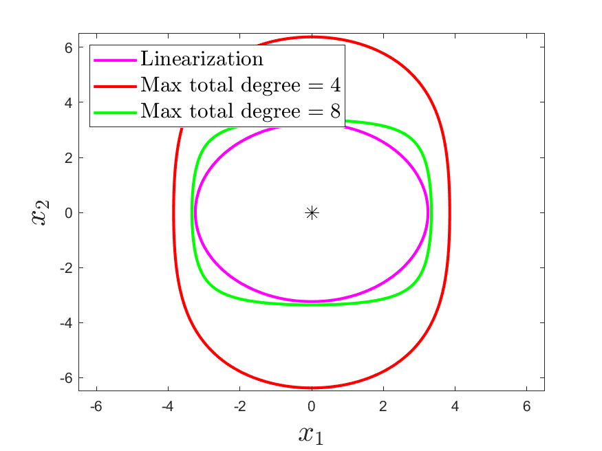
Figure 1: For the switched system (46) with $\displaystyle a=1$ and $\displaystyle b=c=-0.1$, the region of attraction is estimated with the quadratic CLF $\displaystyle V(x_{1},x_{2})=x_{1}^{2}+x_{2}^{2}$ (magenta curve), with the CLF (47) truncated to the total degree 4 (i.e. $\displaystyle k_{max}=5$) (red curve), and with (47) truncated to the total degree 8 (i.e. $\displaystyle k_{max}=14$) (green curve).

4.2 Illustration 2: analytic vector fields

The following example is inspired from [1] and [13].

Consider the switched system defined by the vector fields

(48) $$\begin{array}[]{rcl}F^{(1)}(x_{1},x_{2})&=&\left(-x_{1}+\eta\sin^{2}(x_{1})x_{2}^{2},-x_{2}\right)\\ F^{(2)}(x_{1},x_{2})&=&\left(-x_{1}+\eta\cos^{2}(x_{1})x_{2}^{2},-x_{2}\right),\end{array}$$

with $\displaystyle\eta\in]0,1]$. Both subsystems possess an equilibrium at the origin, which is globally asymptotically stable in $\displaystyle\mathbb{R}^{2}$ (see similar arguments as in [13]). For all $\displaystyle\rho\leq 1$, the square $\displaystyle\mathbb{X}^{2}(\rho)$ is invariant with respect to the flows of $\displaystyle F^{(i)}$. Indeed, we have

• $\displaystyle|x_{1}|=\rho\Rightarrow F^{(1)}_{1}(x)x_{1}=-\rho+\eta x_{1}x_{2}^{2}\sin^{2}(x_{1})<0$ since

  $$\left|\eta x_{1}x_{2}^{2}\sin^{2}(x_{1})\right|\leq\eta\rho\left|x_{2}^{2}\right|<\eta\rho^{3}\leq\rho.$$

• $\displaystyle|x_{2}|=1\Rightarrow F^{(1)}_{2}(x)x_{2}=-\rho<0$.

The same result follows for $\displaystyle F^{(2)}$. The Taylor expansion of the vector fields yields

$$\displaystyle F^{(1)}(x) \displaystyle= \displaystyle\left(-x_{1}+\eta\sum_{p=1}^{\infty}\dfrac{(-1)^{p+1}2^{2p-1}}{(2p)!}x_{1}^{2p}x_{2}^{2},-x_{2}\right)$$

$$\displaystyle F^{(2)}(x) \displaystyle= \displaystyle\left(-x_{1}+\eta x_{2}^{2}+\eta\sum_{p=1}^{\infty}\dfrac{(-1)^{p}2^{2p-1}}{(2p)!}x_{1}^{2p}x_{2}^{2},-x_{2}\right).$$

According to (14), the entries of the Koopman matrices $\displaystyle\bar{L}_{F^{(1)}}$ and $\displaystyle\bar{L}_{F^{(2)}}$ are given by

$$\langle L_{F^{(1)}}e_{k},e_{j}\rangle=\begin{cases}-\left|\alpha(k)\right|&\mbox{if }k=j\\ \eta\alpha_{1}(k)\,\dfrac{(-1)^{p+1}2^{2p-1}}{(2p)!}&\mbox{if }\alpha_{1}(k)=\alpha_{1}(j)+1-2p\geq 0\text{ and }\alpha_{2}(k)=\alpha_{2}(j)-2\geq 0\\ 0&\mbox{otherwise }\end{cases}$$

and

$$\langle L_{F^{(2)}}e_{k},e_{j}\rangle=\begin{cases}-\left|\alpha(k)\right|&\mbox{if }k=j\\ \eta\alpha_{1}(k)&\mbox{if }\alpha_{1}(k)=\alpha_{1}(j)+1\text{ and }\alpha_{2}(k)=\alpha_{2}(j)-2\geq 0\\ \eta\alpha_{1}(k)\,\dfrac{(-1)^{p}2^{2p-1}}{(2p)!}&\mbox{if }\alpha_{1}(k)=\alpha_{1}(j)+1-2p\geq 0\text{ and }\alpha_{2}(k)=\alpha_{2}(j)-2\geq 0\\ 0&\mbox{otherwise }\end{cases}$$

where $\displaystyle p=1,\cdots,\left\lfloor\frac{\alpha_{1}(j)-1}{2}\right\rfloor$. This implies that we have

(49) $$\begin{array}[]{l}\sum_{l=1}^{\infty}\left|\left\langle L_{F^{(1)}}e_{l},e_{j}\right\rangle\right|=\left|\alpha(j)\right|+\eta\sum_{l=1}^{\lfloor\frac{\alpha_{1}(j)-1}{2}\rfloor}\dfrac{(\alpha_{1}(j)+1-2l)2^{2l-1}}{(2l)!}\\ \sum_{l=1}^{\infty}\left|\left\langle L_{F^{(2)}}e_{l},e_{j}\right\rangle\right|=\left|\alpha(j)\right|+\eta\left(\alpha_{1}(j)+1\right)+\eta\sum_{l=1}^{\lfloor\frac{\alpha_{1}(j)-1}{2}\rfloor}\dfrac{(\alpha_{1}(j)+1-2l)2^{2l-1}}{(2l)!}\\ \sum_{l=1}^{\infty}\left|\left\langle L_{F^{(1)}}e_{k},e_{l}\right\rangle\right|=\left|\alpha(k)\right|+\eta\alpha_{1}(k)\sum_{p=1}^{\infty}\dfrac{2^{2p-1}}{(2p)!}=\left|\alpha(k)\right|+\eta\alpha_{1}(k)\frac{\cosh(2)-1}{2}\\ \sum_{l=1}^{\infty}\left|\left\langle L_{F^{(2)}}e_{k},e_{l}\right\rangle\right|=\left|\alpha(k)\right|+\eta\alpha_{1}(k)\left(1+\sum_{p=1}^{\infty}\dfrac{2^{2p-1}}{(2p)!}\right)=\left|\alpha(k)\right|+\eta\alpha_{1}(k)\frac{\cosh(2)+1}{2}.\end{array}$$

Since the Jacobian matrices $\displaystyle JF^{(i)}(0)$ are diagonal, the conditions (40) and (41) are trivially satisfied (with $\displaystyle\xi$ arbitrarily small). Moreover, we observe from (49) that $\displaystyle\sum_{l=1}^{\infty}\left|\left\langle L_{F^{(1)}}e_{l},e_{j}\right\rangle\right|\leq\sum_{l=1}^{\infty}\left|\left\langle L_{F^{(2)}}e_{l},e_{j}\right\rangle\right|$ and $\displaystyle\sum_{l=1}^{\infty}\left|\left\langle L_{F^{(1)}}e_{k},e_{l}\right\rangle\right|\leq\sum_{l=1}^{\infty}\left|\left\langle L_{F^{(2)}}e_{k},e_{l}\right\rangle\right|$ for all $\displaystyle k,j$. It follows that, with $\displaystyle\kappa$ arbitrarily close to $\displaystyle 1$, condition (42) can be rewritten as

$$\limsup_{j\in\mathbb{N}}\max_{k=1,\dots,j-1}\dfrac{\sum_{l=1}^{\infty}\left|\left\langle L_{F^{(2)}}e_{l},e_{j}\right\rangle\right|\sum_{l=1}^{\infty}\left|\left\langle L_{F^{(2)}}e_{k},e_{l}\right\rangle\right|}{\left|\Re\left(\left\langle L_{F^{(2)}}e_{j},e_{j}\right\rangle\right)\right|\left|\Re\left(\left\langle L_{F^{(2)}}e_{k},e_{k}\right\rangle\right)\right|}<\frac{1}{\rho^{2}},$$

which is verified for $\displaystyle\rho=\left(1+\frac{\eta}{2}\left(\cosh(2)+1\right)\right)^{-1}$. Indeed, from (49), we have

$$\displaystyle\sum_{l=1}^{\infty}\left|\left\langle L_{F^{(2)}}e_{l},e_{j}\right\rangle\right| \displaystyle< \displaystyle\left|\alpha(j)\right|+\eta\left(\alpha_{1}(j)+1\right)\left(1+\sum_{l=1}^{\infty}\dfrac{2^{2l-1}}{(2l)!}\right)$$

$$\displaystyle= \displaystyle\left|\alpha(j)\right|+\eta\left(\alpha_{1}(j)+1\right)\frac{\cosh(2)+1}{2}$$

$$\displaystyle\leq \displaystyle\left|\alpha(j)\right|\left(1+\frac{\eta}{2}\left(\cosh(2)+1\right)\right).$$

and

$$\sum_{l=1}^{\infty}\left|\left\langle L_{F^{(2)}}e_{k},e_{l}\right\rangle\right|\leq\left|\alpha(k)\right|\left(1+\frac{\eta}{2}\left(\cosh(2)+1\right)\right).$$

It follows from Corollary 3.17 that the switched system is GUAS on $\displaystyle\mathbb{X}^{2}(\rho)$. See Figure 2 for the different values of $\displaystyle\rho$ depending on $\displaystyle\eta$.

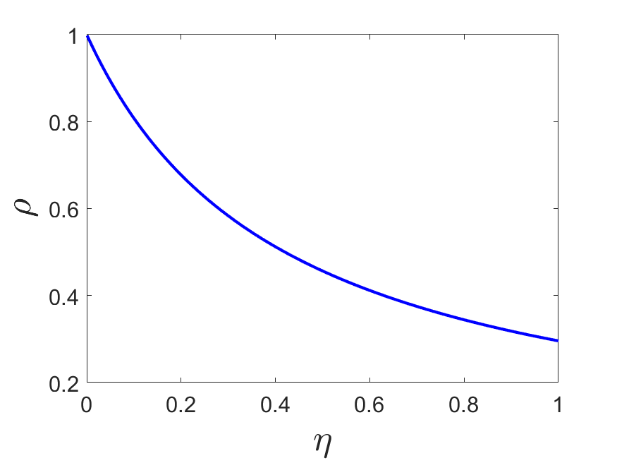
Figure 2: The switched system is shown to be GUAS on a hypercube of edge length $\displaystyle 2\rho$ that depends on the parameter $\displaystyle\eta$.

As shown in Remark 3.19, we have the candidate CLF

(50) $$V(x)=\sum_{k=1}^{k_{max}}Q^{2|\alpha(k)|}\left|x^{\alpha(k)}\right|^{2}$$

where $\displaystyle Q=1/\rho$. The corresponding estimation of the region of attraction is shown in Figure 3 and can be compared to the (smaller) approximation obtained with a quadratic CLF computed for the linearized switched system.

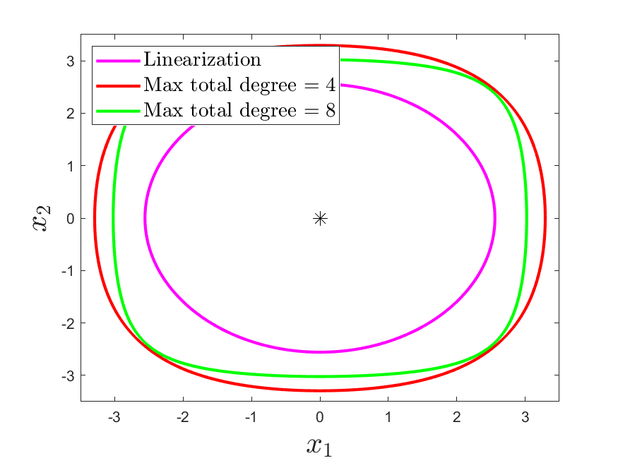
Figure 3: For the switched system (48) with $\displaystyle\eta=1$, the region of attraction is estimated with the quadratic CLF $\displaystyle V(x_{1},x_{2})=x_{1}^{2}+x_{2}^{2}$ (magenta curve), with the CLF (50) truncated to the total degree 4 ($\displaystyle k_{max}=5$) (red curve), and with (50) truncated to the total degree 8 ($\displaystyle k_{max}=14$) (green curve).

5 Conclusion and perspectives

This paper provides new advances on the uniform stability problem for switched nonlinear systems satisfying Lie-algebraic solvability conditions. First, we have shown that the solvability condition on nonlinear vector fields does not guarantee the existence of a common invariant flag and, instead, we have imposed the solvability condition only on the linear part of the vector fields. Then we have constructed a common Lyapunov functional for an equivalent infinite-dimensional switched linear system obtained with the adjoint of the Koopman generator on the Hardy space of the polydisk (or on the real hypercube). Finally we have derived a common Lyapunov function via evaluation functionals to prove that specific switched nonlinear systems are uniformly globally asymptotically stable on invariant sets. Our results heavily rely on the Koopman operator framework, which appears to be a valid tool to tackle theoretical questions from a novel angle.

We envision several perspectives for future research. Our results apply to specific types of switched nonlinear systems within the frame of Lie-algebraic solvability conditions. They could be extended to more general dynamics, including dynamics that possess a limit cycle or a general attractor. In the same line, the Koopman operator-based techniques developed in this paper could be applied to other types of stability than uniform stability. More importantly, the obtained stability results are limited to bounded invariant sets, mainly due to the convergence properties of the Lyapunov functions and the very definition of the Hardy space on the polydisk (or on the real hypercube). We envision that these results could possibly be adapted to infer global stability in $\displaystyle\mathbb{R}^{n}$. Finally, our results are not restricted to switched systems and have direct implications in the global stability properties of nonlinear dynamical systems, which will be investigated in a future publication.

Appendix A General theorems

We recall here some general results that are used in the proofs of our results.

Theorem A.1 (Maximum Modulus Principle for bounded domains [35]).

Let $\displaystyle D^{n}\subset\mathbb{C}^{n}$ be a bounded domain and $\displaystyle f:\overline{D^{n}}\rightarrow\mathbb{C}$ be a continuous function, whose restriction to $\displaystyle D^{n}$ is holomorphic. Then $\displaystyle|f|$ attains a maximum on the boundary $\displaystyle\partial D^{n}$.

Theorem A.2 (Abel’s multidimensional lemma [35] p.36).

Let $\displaystyle\sum_{\alpha\in\mathbb{N}^{n}}a_{\alpha}z^{\alpha}$ be a power series. If there exist $\displaystyle r\in\mathbb{C}^{n}$ such that $\displaystyle\sup_{\alpha\in\mathbb{N}^{n}}\left|a_{\alpha}r^{\alpha}\right|<\infty$, then the series $\displaystyle\sum_{\alpha\in\mathbb{N}^{n}}a_{\alpha}z^{\alpha}$ is normally convergent for all $\displaystyle z\in\mathbb{C}^{n}$ such that $\displaystyle|z_{1}|<|r_{1}|,\,\cdots,|z_{n}|<|r_{n}|$.

Theorem A.3 (Weierstrass’s M-test).

Let $\displaystyle\sum_{k=1}^{+\infty}f_{n}(z)$ be a series of functions on a domain $\displaystyle D^{n}$ of $\displaystyle\mathbb{C}^{n}$. If there exists a sequence of real numbers $\displaystyle M_{k}$ such that

• $\displaystyle M_{k}>0$ for all $\displaystyle k$,

• the numerical series $\displaystyle\sum_{k=1}^{+\infty}M_{k}$ is convergent and

• $\displaystyle\forall k$, $\displaystyle\forall z\in D^{n}$, $\displaystyle\left|f_{k}(z)\right|\leq M_{k}$.

Then the series $\displaystyle\sum_{k=1}^{+\infty}f_{n}(z)$ is absolutely and uniformly convergent on $\displaystyle D^{n}$.

Theorem A.4 (Lie’s theorem [8] p.49).

Let $\displaystyle X$ be a nonzero $\displaystyle n$-complex vector space, and $\displaystyle\mathfrak{g}$ be a solvable Lie subalgebra of the Lie algebra of $\displaystyle n\times n$ complex matrices. Then $\displaystyle X$ has a basis $\displaystyle(v_{1},\dots,v_{n})$ with respect to which every element of $\displaystyle\mathfrak{g}$ has an upper triangular form.

References

- [1] D. Angeli and D. Liberzon, A note on uniform global asymptotic stability of nonlinear switched systems in triangular form, in Proc. 14th Int. Symp. on Mathematical Theory of Networks and Systems (MTNS), 2000.
- [2] V. I. Arnold, Geometrical methods in the theory of ordinary differential equations, vol. 250, Springer Science & Business Media, 2012.
- [3] M. Budišić, R. Mohr, and I. Mezić, Applied Koopmanism, Chaos: An Interdisciplinary Journal of Nonlinear Science, 22 (2012), p. 047510.
- [4] R.-Y. Chen and Z.-H. Zhou, Parametric representation of infinitesimal generators on the polydisk, Complex Analysis and Operator Theory, 10 (2016), pp. 725–735.
- [5] M. Contreras, C. De Fabritiis, and S. Díaz-Madrigal, Semigroups of holomorphic functions in the polydisk, Proceedings of the American Mathematical Society, 139 (2011), pp. 1617–1624.
- [6] C. Dubi, An algorithmic approach to simultaneous triangularization, Linear Algebra and its Applications, 430 (2009), pp. 2975–2981.
- [7] K.-J. Engel, R. Nagel, and S. Brendle, One-parameter semigroups for linear evolution equations, vol. 194, Springer, 2000.
- [8] K. Erdmann and M. J. Wildon, Introduction to Lie algebras, vol. 122, Springer, 2006.
- [9] P. Gaspard, G. Nicolis, A. Provata, and S. Tasaki, Spectral signature of the pitchfork bifurcation: Liouville equation approach, Physical Review E, 51 (1995), p. 74.
- [10] M. Ikeda, I. Ishikawa, and C. Schlosser, Koopman and Perron–Frobenius operators on reproducing kernel Banach spaces, Chaos: An Interdisciplinary Journal of Nonlinear Science, 32 (2022), p. 123143.
- [11] A. Katavolos and H. Radjavi, Simultaneous triangularization of operators on a banach space, Journal of the London Mathematical Society, 2 (1990), pp. 547–554.
- [12] A. Lasota and M. C. Mackey, Chaos, fractals, and noise: stochastic aspects of dynamics, vol. 97, Springer Science & Business Media, 1998.
- [13] D. Liberzon, Switching in systems and control, vol. 190, Springer, 2003.
- [14] D. Liberzon, Lie algebras and stability of switched nonlinear systems, Princeton University Press Princeton, NJ/Oxford, 2004, pp. 203–207.
- [15] D. Liberzon, Switched systems : Stability analysis and control synthesis, 2013.
- [16] D. Liberzon, Commutation relations and stability of switched systems: a personal history, arXiv preprint arXiv:2304.11155, (2023).
- [17] D. Liberzon, J. P. Hespanha, and A. S. Morse, Stability of switched systems: a Lie-algebraic condition, Systems & Control Letters, 37 (1999), pp. 117–122.
- [18] D. Liberzon and A. S. Morse, Basic problems in stability and design of switched systems, IEEE control systems magazine, 19 (1999), pp. 59–70.
- [19] J. L. Mancilla-Aguilar, A condition for the stability of switched nonlinear systems, IEEE Transactions on Automatic Control, 45 (2000), pp. 2077–2079.
- [20] M. Margaliot and D. Liberzon, Lie-algebraic stability conditions for nonlinear switched systems and differential inclusions, Systems & control letters, 55 (2006), pp. 8–16.
- [21] A. Mauroy and I. Mezić, Global stability analysis using the eigenfunctions of the Koopman operator, IEEE Transactions on Automatic Control, 61 (2016), pp. 3356–3369.
- [22] A. Mauroy, I. Mezić, and J. Moehlis, Isostables, isochrons, and Koopman spectrum for the action–angle representation of stable fixed point dynamics, Physica D: Nonlinear Phenomena, 261 (2013), pp. 19–30.
- [23] A. Mauroy, Y. Susuki, and I. Mezić, Koopman operator in systems and control, Springer, 2020.
- [24] I. Mezić, Spectral properties of dynamical systems, model reduction and decompositions, Nonlinear Dynamics, 41 (2005), pp. 309–325.
- [25] I. Mezić, Analysis of fluid flows via spectral properties of the Koopman operator, Annual Review of Fluid Mechanics, 45 (2013), pp. 357–378.
- [26] Y. Mori, T. Mori, and Y. Kuroe, A solution to the common Lyapunov function problem for continuous-time systems, in Proceedings of the 36th IEEE Conference on Decision and Control, vol. 4, 1997, pp. 3530–3531 vol.4, https://doi.org/10.1109/CDC.1997.652397.
- [27] K. S. Narendra and J. Balakrishnan, A common Lyapunov function for stable lti systems with commuting a-matrices, IEEE Transactions on automatic control, 39 (1994), pp. 2469–2471.
- [28] V. I. Paulsen and M. Raghupathi, An introduction to the theory of reproducing kernel Hilbert spaces, vol. 152, Cambridge university press, 2016.
- [29] J. A. Rosenfeld, R. Kamalapurkar, L. F. Gruss, and T. T. Johnson, Dynamic mode decomposition for continuous time systems with the Liouville operator, Journal of Nonlinear Science, 32 (2022), pp. 1–30.
- [30] J. A. Rosenfeld, R. Kamalapurkar, B. Russo, and T. T. Johnson, Occupation kernels and densely defined Liouville operators for system identification, in 2019 IEEE 58th Conference on Decision and Control (CDC), IEEE, 2019, pp. 6455–6460.
- [31] J. A. Rosenfeld, B. Russo, R. Kamalapurkar, and T. T. Johnson, The occupation kernel method for nonlinear system identification, arXiv preprint arXiv:1909.11792, (2019).
- [32] W. Rudin, Function Theory in Polydiscs, Mathematics lecture note series, W. A. Benjamin, 1969, https://books.google.be/books?id=9waoAAAAIAAJ.
- [33] W. Rudin, Function theory in the unit ball of , Springer Science & Business Media, 2008.
- [34] B. P. Russo and J. A. Rosenfeld, Liouville operators over the Hardy space, Journal of Mathematical Analysis and Applications, 508 (2022), p. 125854.
- [35] V. Scheidemann, Introduction to complex analysis in several variables, Springer, 2005.
- [36] J. H. Shapiro, Composition operators: and classical function theory, Springer Science & Business Media, 2012.
- [37] Y. Sharon and M. Margaliot, Third-order nilpotency, finite switchings and asymptotic stability, in Proceedings of the 44th IEEE Conference on Decision and Control, IEEE, 2005, pp. 5415–5420.
- [38] H. Shim, D. Noh, and J. H. Seo, Common Lyapunov function for exponentially stable nonlinear systems, 2001.
- [39] R. Shorten and K. Narendra, On the stability and existence of common Lyapunov functions for stable linear switching systems, in Proceedings of the 37th IEEE Conference on Decision and Control (Cat. No. 98CH36171), vol. 4, IEEE, 1998, pp. 3723–3724.
- [40] R. Shorten, F. Wirth, O. Mason, K. Wulff, and C. King, Stability criteria for switched and hybrid systems, SIAM review, 49 (2007), pp. 545–592.
- [41] I. Steinwart and A. Christmann, Support vector machines, Springer Science & Business Media, 2008.
- [42] L. Vu and D. Liberzon, Common Lyapunov functions for families of commuting nonlinear systems, Systems & control letters, 54 (2005), pp. 405–416.
- [43] C. M. Zagabe and A. Mauroy, Switched nonlinear systems in the Koopman operator framework: Toward a Lie-algebraic condition for uniform stability, in 2021 European Control Conference (ECC), IEEE, 2021, pp. 281–286.