Application of Causal Inference Techniques to the Maximum Weight Independent Set Problem

Abstract

A powerful technique for solving combinatorial optimization problems is to reduce the search space without compromising the solution quality by exploring intrinsic mathematical properties of the problems. For the maximum weight independent set (MWIS) problem, using an upper bound lemma which says the weight of any independent set not contained in the MWIS is bounded from above by the weight of the intersection of its closed neighbor set and the MWIS, we give two extension theorems — independent set extension theorem and vertex cover extension theorem. With them at our disposal, two types of causal inference techniques (CITs) are proposed on the assumption that a vertex is strongly reducible (included or not included in all MWISs) or reducible (contained or not contained in a MWIS). One is a strongly reducible state-preserving technique, which extends a strongly reducible vertex into a vertex set where all vertices have the same strong reducibility. The other, as a reducible state-preserving technique, extends a reducible vertex into a vertex set with the same reducibility as that vertex and creates some weighted packing constraints to narrow the search space. Numerical experiments show that our CITs can help reduction algorithms find much smaller remaining graphs, improve the ability of exact algorithms to find the optimal solutions and help heuristic algorithms produce approximate solutions of better quality. In particular, detailed tests on $12$ representative graphs generated from datasets in Network Data Repository demonstrate that, compared to the state-of-the-art algorithms, the size of remaining graphs is further reduced by more than $32.6\%$, and the number of solvable instances is increased from $1$ to $5$.

AMS subject classifications: 05C69; 68W40; 90C06; 90C27; 90C57

Keywords: maximum weight independent set; independent set extension; vertex cover extension; causal inference techniques; reduction algorithm; exact algorithm; heuristic algorithm; Network Data Repository.

1 Introduction

Let $G=(V,E,w)$ be an undirected vertex-weighted graph, where each vertex $v\in V$ is associated with a weight $w(v)\in\mathbb{R}^{+}$. A subset $I\subseteq V$ is called an independent set if its vertices are pairwise non-adjacent, and the vertex cover of graph $G$ is a subset of vertices $VC\subseteq V$ such that every edge $e\in E$ is incident to at least one vertex in subset $VC$. Independent set and vertex cover are two complementary concepts in graph and can be transformed into each other on demand [29]. The maximum weight independent set (MWIS) problem is to find the independent set of largest weight among all possible independent sets and the weight of a MWIS of graph $G$ is denoted by $\alpha_{w}(G)$, while the minimum weight vertex cover (MWVC) problem asks for the vertex cover with the minimum weight. Furthermore, if subset $I\subseteq V$ is a MWIS, then subset $VC=V\backslash I$ is a MWVC, and vice versa [6, 29]. The MWIS problem is an extension of the maximum independent set (MIS) problem, which is a classic NP-hard problem [13, 9]. It can be applied to various real-world problems, such as information retrieval [4], computer vision [12], combinatorial auction problem [29] and dynamic map labeling problem [17]. Due to its wide range of practical applications, the research on efficient algorithms for computing the MWIS is of great significance. Most previous work are focused on heuristic algorithms to find near-optimal solutions in reasonable time [24, 20, 6, 18], while exact algorithms, usually referring to Branch-and-Bound (B&B) methods [3, 26, 2, 22], become infeasible when the size of problem increases.

Recently, it has been well demonstrated that reduction rules (a.k.a. kernelization) are very effective in practice for solving the MIS problem [25]. These rules mine the structural properties of underlying graph and reduce the search space by such as removing vertices, contracting subgraphs, restricting the set of independent sets, etc., to produce a smaller kernel graph such that the MIS of the original graph can be recovered from the MIS of the kernel. After integrating them, some state-of-the-art exact solvers are able to solve the MIS problem on many large real networks [11]. These solvers can be usually divided into two types: One performs the kernelization only once and runs the B&B algorithm [23, 16] on the kernelized instance, while the other joins hands with the Branch-and-Reduce (B&R) algorithm [19] and performs reduction in every branch of the search tree. As for those instances that can’t be solved exactly, high-quality solutions can be found by combining kernelization with local search [8, 10]. Moreover, when a vertex is selected for branching in the branching process of the B&R algorithm, if it is assumed to be in all MISs, then its satellite set will also be in all MISs [14], while its mirror set will be removed directly from the graph, if it is assumed not to be in all MISs [13]. Further, a conflict analysis on the assumption that a vertex is in all MISs can be also plugged in to find some contradictions and the concept of “unconfined/confined vertices” was introduced [28]. Later, an auxiliary constraint called packing constraint was proposed to accelerate the B&R algorithm by simply exploring branches that satisfy all packing constraints [1]. The central idea behind all these attempts for the MIS problem involves a state-preserving technique which starts from a vertex, named the starting vertex for convenience, and then finds a vertex set with the same state as the starting vertex to reduce the search space, thereby implying that some subsequent operations can be implemented on the resulting vertex set instead of only on the starting vertex. For the MWIS problem, similar state-preserving techniques are rarely used except for a recent work using unconfined/confined vertices [27], though some simple and fast reduction rules have been used in B&R algorithms [15, 27]. To this end, we devote ourselves into developing state-preserving techniques for the MWIS problem in this work. The state of the starting vertex we consider can be

• strongly reducible, meaning that the vertex is included in all MWISs/MWVCs; or

• reducible, meaning that the vertex is contained in a MWIS/MWVC.

Considering that the assumed state of the starting vertex must be used to analyze its local structure to obtain inference results, these targeted state-preserving techniques are called causal inference techniques (CITs). Inspired by their success in solving the MIS problem, we will systematically develop CITs to solve the MWIS problem by analyzing intrinsic mathematical properties of underlying graph. More specifically, our main contributions are in three aspects as follows.

First, by virtue of the upper bound lemma, i.e., the weight of any independent set not contained in the MWIS is bounded from above by the weight of the intersection of its closed neighbor set with the MWIS, two extension theorems are developed. With them, we propose a series of CITs which have been rarely used previously in the MWIS problem. According to the state of the starting vertex, our CITs can be divided into two categories. The first type is a strongly reducible state-preserving technique. We first assume that the starting vertex is strongly reducible, and then try to extend this vertex to obtain a vertex set with the same strong reducibility. If the upper bound lemma is not satisfied in this process, then this contradicts the assumption, and the starting vertex can be removed from the graph directly. Otherwise, combined with the state-preserving result obtained from the previous process, we continue to search for a set called the simultaneous set, which is either included in a MWIS or contained in a MWVC. The second type is a reducible state-preserving technique. Under the assumption that the starting vertex is reducible, a vertex set with the same reducibility can be obtained by extending from this vertex. Moreover, if this vertex is selected for branching in the B&R algorithm, with the upper bound lemma, an inequality constraint called weight packing constraint will be created to restrict subsequent searches.

Next, according to the characteristics of the proposed CITs, we integrate them into the existing algorithmic framework. The first type of CIT can be used to design reduction rules to simplify graph. These reduction rules are integrated into the existing reduction algorithm. In the B&R algorithm, when a vertex is selected to branch, a vertex set and a weight packing constraint depending on the assumed state of the vertex can be obtained from state-preserving results of two types of CITs. The vertex set is used to further simplify the corresponding branch, while we can prune branches that violate constraints and simplify the graph by maintaining all created weight packing constraints. During the local search process of the heuristic algorithm, when the state of a vertex needs to be changed, all vertex states in the vertex set obtained by the second type of CIT will also be modified to be the same as that vertex, which expands the area of local search and improves the ability of local search to find better local optima.

Numerical experiments on $12$ representative graphs generated from datasets in Network Data Repository show that the performance of various algorithms is greatly improved after integrating our CITs. The size of the kernel obtained by the resulting reduction algorithm is greatly reduced. In addition, compared to the state-of-the-art exact algorithm, the number of solvable instances have been increased from $1$ to $5$. And the ability of the heuristic algorithm to find better local optimal solutions is significantly improved. These experimental results form the third major contribution of this paper.

$G=(V,E,w)$	an undirected vertex-weight graph $G$ with vertex set $V$, edge set $E$ and vertex weight function $w:V\rightarrow\mathbb{R}^{+}$
$N(v)=\{u\in V|\{u,v\}\in E\}$	the neighbor set of vertex $v$	$N[v]=N(v)\cup\{v\}$	the closed neighbor set of vertex $v$
$N(S)=(\bigcup\limits_{v\in S}N(v))\backslash S$	the open neighbor set of set $S$	$N[S]=N(S)\cup\{S\}$	the closed neighbor set of set $S$
$|S|$	the size of set $S$	$w(S)=\sum\limits_{v\in S}w(v)$	the weight of all vertices in set $S$
$d(v)$	the degree of a vertex $v$	dist$(u,v)$	the minimum number of edges in the path from vertex $u$ to vertex $v$
$N^{l}(v)=\{u|$ dist$(u,v)=l\}$	the set of vertices at distance $l$ from vertex $v$, in particular, $N^{1}(v)=N(v)$	$G[S]=(S,E_{S},w)$, $\forall e=\{u,v\}\in E_{S}$, $u,v\in S$	the subgraph induced by a non-empty vertex subset $S$ of $V$
$\alpha(G)$	the size of a MIS of unweight graph $G$	$\alpha_{w}(G)$	the weight of a MWIS of graph $G$
$A_{I}$	the set of all MWISs in graph $G$	$A_{C}$	the set of all MWVCs in graph $G$
$S\blacktriangleleft A_{I}$	set $S$ is an independent set and is included in all MWISs	$C\vartriangleleft A_{C}$	set $C$ is contained in all MWVCs
vertex $v$ is strongly reducible	vertex $v$ is included in all MWISs/MWVCs	vertex $v$ is reducible	vertex $v$ is contained in a MWIS/MWVC
vertex $v$ is strongly inclusive	vertex $v$ is included in all MWISs	vertex $v$ is strongly sheathed	vertex $v$ is contained in all MWVCs
vertex $v$ is inclusive	vertex $v$ is included in a MWIS	vertex $v$ is sheathed	vertex $v$ is contained in a MWVC
set $S$ is strongly inclusive	set $S$ is an independent set and is included in all MWISs	set $S$ is strongly sheathed	set $S$ is contained in all MWVCs
set $S$ is inclusive	set $S$ is an independent set and is included in a MWIS	set $S$ is sheathed	set $S$ is contained in a MWVC
independent set $S$ is strongly exclusive	independent set $S$ is not contained in all MWIS	independent set $S$ is exclusive	independent set $S$ is not contained in a MWIS
a set $S$ called a simultaneous set	set $S$ is either included in a MWIS or contained in a MWVC

Table 1: Notations used throughout the paper.

Relevant notations used in this work are given in Table 1 and the rest of the paper is organized as follows. We present two extension theorems in Section 2 and detail CITs in Section 3. How the CITs are combined with existing algorithmic frameworks is described in Section 4. Extensive numerical tests are carried out in Section 5 to verify the performance improvement of integrating our CITs into existing algorithmic frameworks in terms of efficiency and accuracy. The paper is concluded in Section 6 with a few remarks.

2 Two Extension Theorems

The theoretical cornerstones of CITs in this paper are two extension theorems: independent set extension theorem and vertex cover extension theorem. Before delineating them, we need to have a deep understanding of the local structure of the MWIS and first give the upper bound lemma.

Lemma 2.1 (upper bound lemma).

Let set $I_{C}$ be an independent set in the graph.

• Suppose there is an $I_{w}\in A_{I}$ such that $I_{C}\not\subseteq I_{w}$, then $w(I_{w}\cap N[I_{C}])\geqslant w(I_{C})$ holds.

• Assume that $I_{C}\not\subseteq I,\forall I\in A_{I}$ holds, then it satisfies: $w(I_{C})<w(I\cap N[I_{C}]),\forall I\in A_{I}$.

Proof.

Proof We first prove $(a)$ by contradiction. If not, we can obtain an independent set $I_{w}^{\prime}=(I_{w}\backslash N[I_{C}])\cup(I_{C})$ such that $w(I_{w}^{\prime})=w(I_{w})+w(I_{C})-w(I_{w}\cap N[I_{C}])>w(I_{w})$, a contradiction.

Next, we consider $(b)$. If there is an $I_{1}\in A_{I}$ such that $w(I_{C})\geqslant w(I_{1}\cap N[I_{C}]))$, we can construct an independent set $I^{\prime}_{1}=(I_{1}\backslash N[I_{C}])\cup I_{C}$ satisfying $w(I^{\prime}_{1})=w(I_{1})+w(I_{C})-w(I_{1}\cap N[I_{C}])\geqslant w(I_{1})$. Then $I^{\prime}_{1}\in A_{I}$ and $I_{C}\subseteq I^{\prime}_{1}$, which leads to a contradiction. ∎

The upper bound lemma describes such a property: For any independent set that is (strongly) exclusive, the weight of the intersection of its closed neighbor set with the MWIS is the upper bound on its weight. With it, the independent set extension theorem can be introduced as follows.

Theorem 2.2 (Independent Set Extension Theorem).

Let sets $IS$ and $S$ be two independent sets in the graph.

• Assume that there exists an $I_{w}\in A_{I}$ such that $IS\subseteq I_{w}$. If there is an independent set $IS^{\prime}\subseteq N(IS)$ such that $w(IS^{\prime})>w(IS\cap N(IS^{\prime}))$, then there exists an independent set $IS^{\prime\prime}\subseteq N(IS^{\prime})\backslash N[IS]$ satisfying the inequality: $w(IS^{\prime})\leqslant w(IS\cap N(IS^{\prime}))+w(IS^{\prime\prime})$. In addition, $IS\cup IS^{\prime\prime}\subseteq I_{w}$ if such $IS^{\prime\prime}$ is unique.

• Suppose $S\blacktriangleleft A_{I}$, then for any independent set $S^{\prime}\subseteq N(S)$, there is an independent set $S^{\prime\prime}\subseteq N(S^{\prime})\backslash N[S]$ such that $w(S^{\prime})<w(S\cap N(S^{\prime}))+w(S^{\prime\prime})$. Besides, if such $S^{\prime\prime}$ is unique, then $S\cup S^{\prime\prime}\blacktriangleleft A_{I}$.

Proof.

Proof We first consider the proof of $(a)$, and it is obvious that $IS^{\prime}\not\subseteq I_{w}$. In view of the fact that the relationship between $I_{w}$ and $N[IS^{\prime}]$ satisfies: $I_{w}\cap N[IS^{\prime}]=I_{w}\cap N(IS^{\prime})=(IS\cap N(IS^{\prime}))\cup(I_{w}\cap(N(IS^{\prime})\backslash N[IS]))$ and by the upper bound lemma, we can get: $w(IS\cap N(IS^{\prime}))+w(I_{w}\cap(N(IS^{\prime})\backslash N[IS]))=w(I_{w}\cap N(IS^{\prime}))=w(I_{w}\cap N[IS^{\prime}])\geqslant w(IS^{\prime}).$ Thus, the existence of such $IS^{\prime\prime}$ is proved. Furthermore, assuming that such $IS^{\prime\prime}$ is unique, then $IS^{\prime\prime}=I_{w}\cap(N(IS^{\prime})\backslash N[IS])$ and $IS\cup IS^{\prime\prime}\subseteq I_{w}$.

Similar ideas can be used to prove $(b)$. Obviously $S^{\prime}\not\subseteq I,\forall I\in A_{I}$ holds, so from the upper bound lemma, it can be directly obtained: $\forall I\in A_{I},w(I\cap N[S^{\prime}])>w(S^{\prime})$. Further, by considering that the relationship between $I$ and $N[S^{\prime}]$ satisfies: $I\cap N[S^{\prime}]=I\cap N(S^{\prime})=(S\cap$ $N(S^{\prime}))\cup(I\cap(N(S^{\prime})\backslash N[S]))$, we prove the existence of such $S^{\prime\prime}$. Also, if such $S^{\prime\prime}$ is unique, the following result holds: $S^{\prime\prime}=I\cap(N(S^{\prime})\backslash N[S]),\forall I\in A_{I}$, and then $S\cup S^{\prime\prime}\blacktriangleleft A_{I}$. ∎

The independent set extension theorem gives a method for extending independent set that is (strongly) inclusive: Try to find an independent set to add to the extended independent set, and that independent set is the only one that guarantees that the upper bound lemma is satisfied in the local structure of the extended independent set. Next, with the help of the upper bound lemma, the vertex cover extension theorem is given below.

Theorem 2.3 (Vertex Cover Extension Theorem).

Let sets $IC$ and $C$ be two vertex subsets in the graph.

• Suppose set $IC\subseteq VC_{w}$, then the vertices in $IC$ have the property: $\forall p\in IC$, $w(p)\leqslant\alpha_{w}(G[N(p)\backslash IC])$. Also, for a vertex $v\in IC$ and a vertex $u\in N^{2}(v)$, $IC\cup\{u\}\subseteq VC_{w}$ holds if the inequality $w(v)>\alpha_{w}(G[N(v)\backslash(IC\cup N(u))])$ is satisfied.

• Assume that set $C\vartriangleleft A_{C}$, then $\forall p\in C,w(p)<\alpha_{w}(G[N(p)\backslash C])$ is always satisfied. In addition, if there exists a vertex $v\in C$ and a vertex $u\in N^{2}(v)$ such that $w(v)\geqslant\alpha_{w}(G[N(v)\backslash(C\cup N(u))])$, then $C\cup\{u\}\vartriangleleft A_{C}$.

Proof.

Proof We first consider $(a)$ and let set $I_{w}=V\backslash VC_{w}$. From the upper bound lemma, these results can be directly obtained: $\forall p\in IC,w(p)\leqslant w(I_{w}\cap N[p])=w(I_{w}\cap N(p))\leqslant\alpha_{w}(G[N(p)\backslash IC])$. Also, based on the assumption about $u$ in $(a)$, if $u\in I_{w}$, then $w(v)\leqslant w(I_{w}\cap N[v])=w(I_{w}\cap N(v))\leqslant\alpha_{w}(G[N(v)\backslash(IC\cup N(u))])$, which leads to a contradiction.

Similar methods can be used to prove $(b)$. First, $\forall p\in C,\forall I\in A_{I},w(p)<w(I\cap N[p])=w(I\cap N(p))\leqslant\alpha_{w}(G[N(p)\backslash C])$ can be obtained from the upper bound lemma. Besides, under given conditions about $u$ in $(b)$, if there is an $I^{*}\in A_{I}$ such that $u\in I^{*}$, a contradiction is deduced from $w(p)<w(I^{*}\cap N[p])=w(I^{*}\cap N(p))\leqslant\alpha_{w}(G[N(p)\backslash(C\cup N(u))])$. ∎

The vertex cover extension theorem describes how to expand a set that is (strongly) sheathed: Attempt to find a vertex that satisfies the condition that after removing its neighbor set, the upper bound lemma is not satisfied in the local structure of the expanded set. If such a vertex is found, it is directly added to the expanded set.

3 Causal Inference Techniques

In this section, with the help of the upper bound lemma and two extension theorems, we give the CITs used in this paper. Our CITs can be divided into two types: The first type is a strongly reducible state-preserving technique introduced in Section 3.1, while the second type is a reducible state-preserving technique shown in Section 3.2.

3.1 Strongly reducible state-preserving technique

The strongly reducible state-preserving technique exploits the assumption that a vertex is strongly reducible, and the assumed state of the vertex can be divided into two cases: The vertex is assumed to be strongly inclusive or is assumed to be strongly sheathed. We first consider the assumption that a vertex is strongly inclusive and give the following definition.

Definition 3.1.

Let set $S$ be an independent set in the graph. If a vertex $u\in N(S)$ such that $w(u)\geqslant w(S\cap N(u))$, we call it a child of set $S$. A child $u$ is called an extending child if and only if there exists a unique independent set $S^{*}\subseteq N(u)\backslash N[S]$ such that $w(u)<w(S\cap N(u))+w(S^{*})$ and vertex set $S^{*}$ is called a satellite set of set $S$.

On the basis of Definition 3.1, with the assumption that a vertex is strongly inclusive, the concept of ‘confined/unconfined vertices’ is given by the following conflict analysis process:

Definition 3.2.

Let $v$ be a vertex in the graph. Suppose set $S:=\{v\}\blacktriangleleft A_{I}$, repeating $(i)$ until $(ii)$ or $(iii)$ holds:

• As long as set $S$ has an extending child in $N(S)$, set $S$ is extended by including the corresponding satellite set into set $S$.

• If a child $u$ such that $w(u)\geqslant w(S\cap N(u))+\alpha_{w}(G[N(u)\backslash N[S]])$ could be found, that is, the upper bound lemma is not satisfied in the local structure of set $S$, then halt and vertex $v$ is called an unconfined vertex.

• If any child is not an extending child, then halt and return set $S_{v}=S$. In this case, vertex $v$ is called a confined vertex and the set $S_{v}$ is called the confining set of vertex $v$.

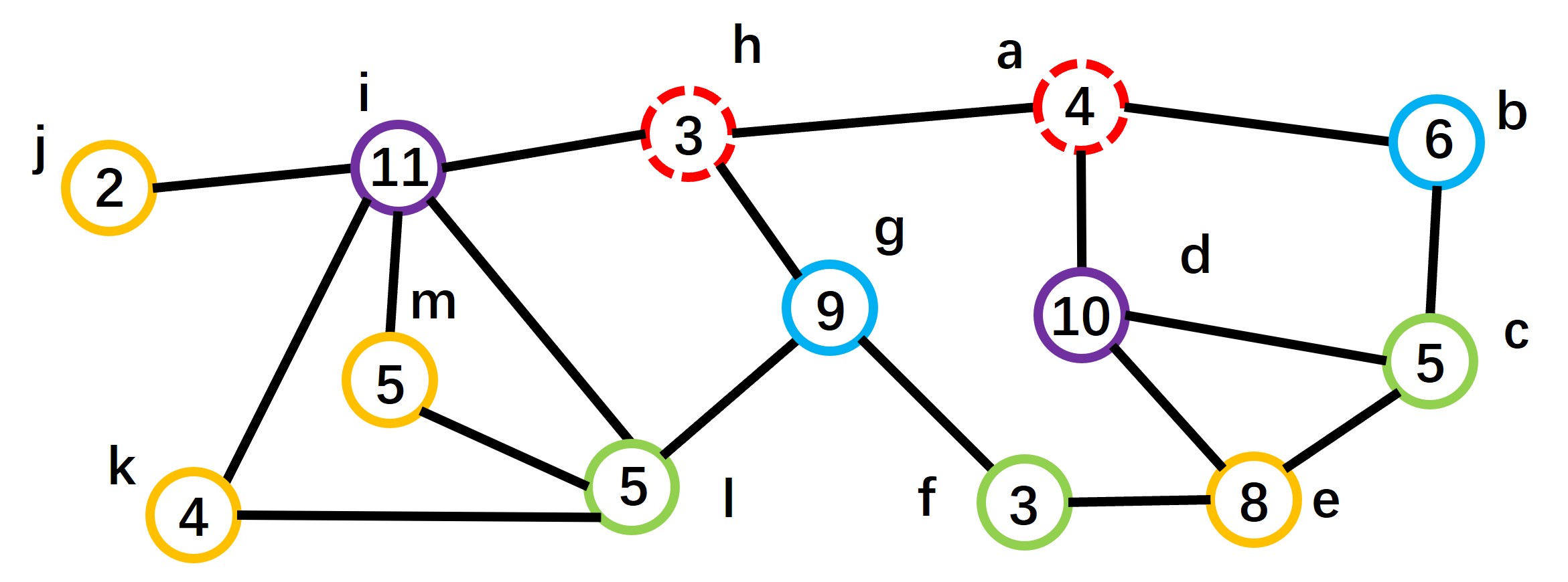
Figure 1: Some examples of unconfined vertices, and a MWIS in this graph is $\{b,d,g,i\}$. Let set $S:=\{a\}$, from Definition 3.1, vertex $b$ is an extending child of set $S$ and set $\{c\}$ is a satellite set of set $S$. Thus, set $S$ can be extended as: $\{a,c\}$. At this time, it can be found that a child $d$ such that $w(d)\geqslant w(S\cap N(d))+\alpha_{w}(G[N(d)\backslash N[S]])$, then halt and conclude that vertex $a$ is an unconfined vertex. Similarly, let set $S:=\{h\}$, then it can be found that vertex $g$ is an extending child of set $S$ and set $\{f,l\}$ is a satellite set of set $S$. So set $S$ can be further expanded as: $\{h,l,f\}$. After that, the child $i$ satisfied: $w(i)\geqslant w(S\cap N(i))+\alpha_{w}(G[N(i)\backslash N[S]])$, hence, vertex $h$ is an unconfined vertex.

Some examples of unconfined vertex are given in Figure 1. By means of the conflict analysis process in Definition 3.2, vertices $a$ and $h$ can be found to be unconfined vertices. It is also worth noting that, by the definition of unconfined vertex given in [27], in Figure 1, only vertex $a$ can be found to be an unconfined vertex. The reason for this is that we further generalize the concept of confined/unconfined vertices in this work. Compared with the definition of extending child $u$ in [27], which requires $|N(u)\backslash N[S]|$ $=1$ and $w(u)<w(N(u)\backslash N(S))$, we can consider the more general case where $N(u)\backslash N[S]$ is an independent set rather than a single vertex, helping us find more unconfined vertices.

Next, we will explore the properties of confined/unconfined vertices. By the conflict analysis process in Definition 3.2 and the independent set extension theorem, set $S$ can be extended under the assumption: set $S:=\{v\}\blacktriangleleft A_{I}$, and set $S\blacktriangleleft A_{I}$ is always satisfied. If vertex $v$ is a unconfined vertex, then the upper bound lemma is not satisfied in the local structure of set $S$, which contradicts set $S\blacktriangleleft A_{I}$. Thus, vertex $v$ is sheathed. Otherwise, then there is a state-preserving result, i.e., the corresponding confining set $S_{v}\blacktriangleleft A_{I}$ holds. Furthermore, suppose two confined vertices $u$, $v$ and the corresponding confining sets $S_{u},S_{v}$ such that $u\in S_{v}$ and $v\in S_{u}$. If $\{v\}\blacktriangleleft A_{I}$, then obviously $\{u\}\blacktriangleleft A_{I}$ holds. If not, vertex $v$ is sheathed in graph $G$. Since $v\in S_{u}$, then vertex $v$ is included in the satellite set of an intermediate state set $S^{\prime}$ of $S_{u}$, which means that in graph $G[V\backslash\{v\}]$, the upper bound lemma is not satisfied in the local structure of set $S^{\prime}$. Thus, by Definition 3.2, vertex $u$ is an unconfined vertex of graph $G[V\backslash\{v\}]$ and is sheathed in this graph. From these analysis results and the symmetry of the relationship between vertex $v$ and vertex $u$, we can know that vertex set $\{u,v\}$ is a simultaneous set. Therefore, the following properties can be obtained:

Corollary 3.3.

Let $v$ is a vertex in the graph.

• If vertex $v$ is an unconfined vertex, then it is sheathed and after deleting it from the graph, the weight of the MWIS in the remaining graph remains unchanged.

• Suppose vertex $v$ is a confined vertex, then either it is sheathed or the corresponding confining set $S_{v}\blacktriangleleft A_{I}$. Moreover, if a vertex $u\in S_{v}$ is also a confined vertex with the corresponding confining set $S_{u}$ and $v\in S_{u}$, then vertex set $\{u,v\}$ is a simultaneous set.

From Corollary 3.3, it can be known that the conflict analysis process in Definition 3.2 can be used to find the vertex that is sheathed or a simultaneous set. These CITs will be used to design reduction rules in Section 4.1. In addition, by the property of confined vertex, a fact is obvious: If confined vertex $v$ such that $\{v\}\blacktriangleleft A_{I}$, then the corresponding confining set $S_{v}\blacktriangleleft A_{I}$. We will exploit this state-preserving result in the B&R algorithm to design a branching rule to search for a solution in Section 4.2.

Next, we proceed to consider the assumption that a vertex is strongly sheathed. In the MIS problem, the notion of mirror is given by means of such an assumption and is very useful in practice [1]. We will generalize the notion of mirror to the MWIS problem: For a vertex $v\in V$, a mirror of vertex $v$ is a vertex $u\in N^{2}(v)$ such that $w(v)\geqslant\alpha_{w}(G[N(v)\backslash N(u)])$.

Remark 3.4.

When the weight of all vertices in the graph is $1$, then $\alpha(G[N(v)\backslash N(u)])=\alpha_{w}(G[N(v)\backslash N(u)])$ $\leqslant w(v)=1$. This means that $N(v)\backslash N(u)$ induces a clique or is an empty set, and this is exactly the definition that vertex $u$ is the mirror of vertex $v$ in the MIS problem.

To make the concept of mirror more practical, we further generalize it to the case of set, which leads to the following definitions:

Definition 3.5.

Let set $C$ be a vertex subset in the graph. If a vertex $v\in C$ satisfies the inequality: $w(v)<\alpha_{w}(G[N(v)\backslash C])$, we call it a father of set $C$. Furthermore, if there exists a vertex $u\in N^{2}(v)$ such that $w(v)\geqslant\alpha_{w}(G[N(v)\backslash(C\cup N(u))])$, then the father $v$ is called an extending father of set $C$ and vertex $u$ is called a mirror of vertex $v$. We use $M(v)$ to denote the set of mirrors of vertex $v$.

By means of Definition 3.5, and under the assumption that a vertex is strongly sheathed, the concept of ‘covered/uncovered vertices’ is given by the following conflict analysis process:

Definition 3.6.

Let $v$ be a vertex in the graph. At the beginning, suppose set $C:=\{v\}\vartriangleleft A_{C}$ and repeating $(i)$ until $(ii)$ or $(iii)$ are met:

• When set $C$ has an extending father, extend set $C$ by including the corresponding set of mirrors to set $C$.

• If there is a vertex $u\in C$ such that $w(u)\geqslant\alpha_{w}(G[N(u)\backslash C])$, in this case, the upper bound lemma is not satisfied, then halt and vertex $v$ is called an uncovered vertex.

• If set $C$ has no extending father, then halt and return set $C_{v}=C$. In this case, vertex $v$ is called a covered vertex and vertex set $C_{v}$ is called the covering set of vertex $v$.

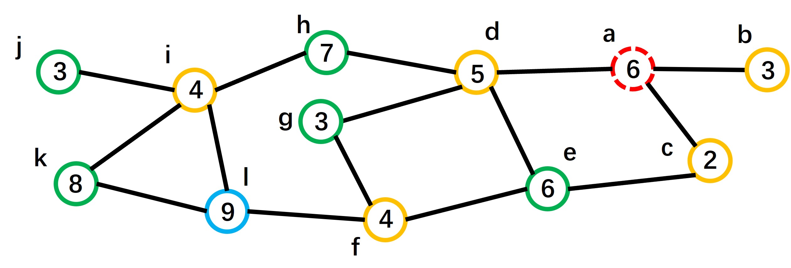
Figure 2: An example of uncovered vertex and a MWIS of this graph is $\{a,e,g,h,j,l\}$. Starting with set $C:=\{a\}$, from Definition 3.5, it can be seen that vertex $a$ is an extending father of set $C$ and set $\{e,g,h\}$ is the mirrors set of vertex $a$. Thus, set $C$ can be extended to: $\{a,e,g,h\}$. Then, vertex $h$ is also an extending father of set $C$ and set $\{j,k,l\}$ is the mirrors set of vertex $h$. So set $C$ can be further expanded as: $\{a,e,g,h,j,k,l\}$. At this time, we find that $w(l)\geqslant\alpha_{w}(G[N(l)\backslash C])$, then halt and conclude that vertex $a$ is uncovered.

An example of uncovered vertex is given in Figure 2 and we find that vertex $a$ is an uncovered vertex. In addition, the properties of uncovered/covered vertices are worth further study. From the vertex cover extension theorem, in the conflict analysis process of Definition 3.6, for any extending father $f$ of set $C$, $\forall u\in M(f)$, if set $C\vartriangleleft A_{C}$, set $C\cup\{u\}\vartriangleleft A_{C}$ always holds. Thus, under the assumption set $C:=\{v\}\vartriangleleft A_{C}$, if vertex $v$ is not an uncovered vertex, then a state-preserving result can be obtained: The corresponding covering set $C_{v}\vartriangleleft A_{C}$. Otherwise, the upper bound lemma is not satisfied in the local structure of set $C$, which contradicts hypothesis set $C\vartriangleleft A_{C}$. So vertex $v$ is inclusive. Also, assume that the two covered vertices $u,v$ and the corresponding covering set $C_{u},C_{v}$ satisfy: $v\not\in N(u)$, $u\in C_{v}$ and $v\in C_{u}$. If vertex $v$ is inclusive, we first remove $N[v]$ from graph $G$. Since $v\in C_{u}$, then vertex $v$ is a mirror of an extending father of an intermediate state set $C^{\prime}$ of set $C_{u}$ and the upper bound lemma cannot be satisfied in graph $G[V\backslash N[v]]$ at this time. Thus, vertex $u$ is an uncovered vertex of graph $G[V\backslash N[v]]$ and is inclusive in this graph. So there exists a MWIS in graph $G$ containing both vertex $v$ and vertex $u$. Moreover, if $\{v\}\vartriangleleft A_{C}$, $\{u\}\vartriangleleft A_{C}$ is clearly satisfied. Thus, from the symmetry of the relationship between vertex $u$ and vertex $v$, it can be known that vertex set $\{u,v\}$ is a simultaneous set. These properties are summarized as follows.

Corollary 3.7.

Let $v$ be a vertex in the graph $G$.

• If vertex $v$ is an uncovered vertex, then it is inclusive. After deleting $N[v]$ from the graph, the weight of the MWIS in the remaining graph satisfies: $\alpha_{w}(G)=\alpha_{w}(G[V\backslash N[v]])+w(v)$.

• If vertex $v$ is a covered vertex. Then, either vertex $v$ is inclusive or the corresponding covering set $C_{v}\vartriangleleft A_{C}$. Also, if another covered vertex $u$ with the corresponding covering set $C_{u}$ satisfies: $v\not\in N(u)$, $u\in C_{v}$ and $v\in C_{u}$, then vertex set $\{u,v\}$ is a simultaneous set.

Corollary 3.7 gives the following results: The conflict analysis process in Definition 3.6 can be applied to find the vertex that is inclusive or a simultaneous set. In Section 4.1, we will use these CITs to design reduction rules. Besides, by the property of covered vertex in $(b)$ of Corollary 3.7, we can know a state-preserving result: if the covered vertex $v$ such that $\{v\}\vartriangleleft A_{C}$, then the corresponding covering set $C_{v}\vartriangleleft A_{C}$.

3.2 Reducible state-preserving technique

Similar to the first type of CIT, the reducible state-preserving technique utilizes the assumption that a vertex is reducible, that is, assumes that a vertex is inclusive or sheathed. With these assumptions, we can give state-preserving results similar to the first type of CIT. Before that, we give the following definition.

Definition 3.8.

Let sets $IS$ and $IC$ be two vertex subsets in the graph and set $IS$ is an independent set.

• A vertex $u\in N(IS)$ is called an inferred child of set $IS$ if it holds that $w(u)>w(IS\cap N(u))$. Further, if there is only a unique independent set $IS^{*}\subseteq N(u)\backslash N[IS]$ that satisfies the inequality: $w(u)\leqslant w(IS\cap N(u))+w(IS^{*})$, we call the inferred child $u$ an inferred extending child of set $IS$ and vertex set $IS^{*}$ is called an inferred satellite set of set $IS$.

• A vertex $v\in IC$ is called an inferred father of set $IC$ if it holds that $w(v)\leqslant\alpha_{w}(G[N(v)\backslash IC])$. An inferred father $v$ is called an inferred extending father of set $IC$ if there exists a vertex $u\in N^{2}(v)$ such that $w(v)>\alpha_{w}(G[N(v)\backslash(IC\cup N(u))])$ and vertex $u$ is called an inferred mirror of vertex $v$. Also, $IM(v)$ is used to denote its set of inferred mirrors.

By virtue of Definition 3.8 and the assumption that a vertex is inclusive or sheathed, we can directly give the definitions of inferred confining set and inferred covering set accordingly.

Definition 3.9.

Suppose there are no unconfined vertex in the graph. Let $v$ be a vertex in the graph. Beginning with the assumption set $IS:=\{v\}\subseteq I_{w}$.

• Only if set $IS$ has an inferred extending child in $N(IS)$, set $IS$ can be extended by including the corresponding inferred satellite set to set $IS$.

• The above process halts if set $IS$ has no inferred extending child in $N(IS)$ and return set $IS_{v}=IS$. We call vertex set $IS_{v}$ is the inferred confining set of vertex $v$.

Definition 3.10.

We assume that there are no uncovered vertex in graph. Let $v$ be a vertex in the graph. Starting with the assumption set $IC:=\{v\}\subseteq VC_{w}$.

• While set $IC$ has an inferred extending father, extend set $IC$ by including the corresponding set of inferred mirrors to set $IC$.

• The above process halts if set $IC$ has no inferred extending father and return set $IC_{v}=IC$. We call vertex set $IC_{v}$ is the inferred covering set of vertex $v$.

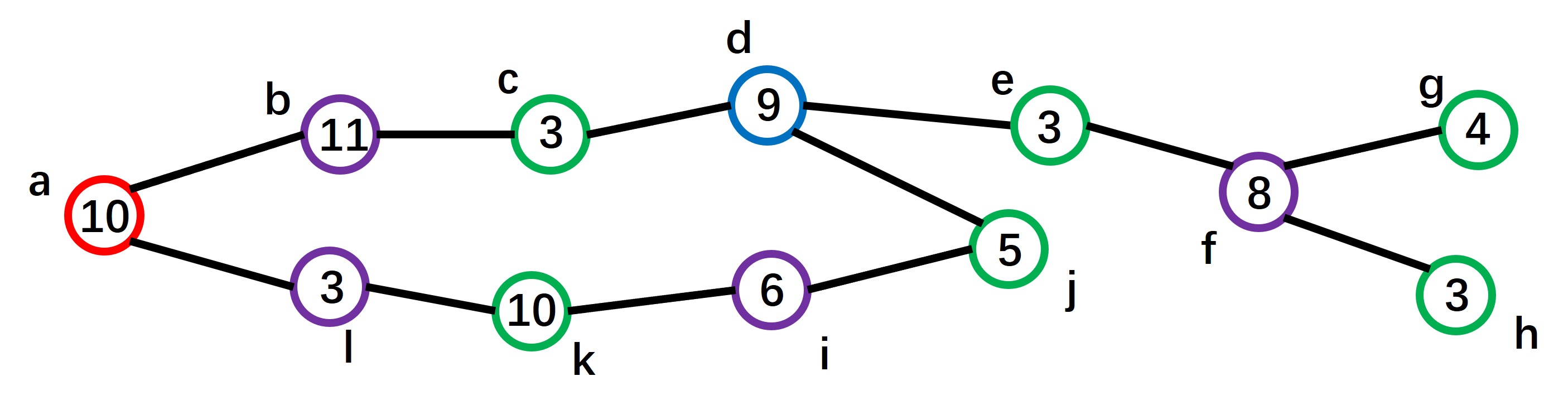
Figure 3: Examples of inferred confining set and inferred covering set. A MWIS for this graph is $\{a,c,e,g,h,j,k\}$. We first search for the inferred confining set $IS_{a}$ of vertex $a$. Let set $IS:=\{a\}$, it can be seen from $(a)$ of Definition 3.8 that vertex $b$ is an inferred extending child of set $IS$ and set $\{c\}$ is an inferred satellite set of set $IS$. Thus, set $IS$ can be extended to: $\{a,c\}$. Further, vertex $d$ is also an inferred extending child of set $IS$ and set $\{e,j\}$ is the corresponding inferred satellite set. So set $IS$ can be further extended to: $\{a,c,e,j\}$. At this time, it can be found that both vertex $f$ and vertex $i$ are inferred extending children of set $IS$. Then, both vertex set $\{g,h\}$ and vertex set $\{k\}$ are the corresponding inferred satellite sets. Finally, the inferred confining set of vertex $a$ can be found as: $IS_{a}=\{a,c,e,j,g,h,k\}$. Furthermore, we continue to search the inferred covering set $IC_{d}$ of vertex $d$. Let set $IC:=\{d\}$, according to $(b)$ of Definition 3.8, vertex $d$ is an extending father of set $IC$ and set $\{b,f,i\}$ is its inferred mirrors set. Then, set $IC$ can be extended as: $\{b,d,f,i\}$. Next, it can be found that vertex $b$ is an extending father of set $IC$ and set $\{l\}$ is its inferred mirrors set. Thus, set $IC$ can be further extended as: $\{b,d,f,i,l\}$. Finally, the inferred covering set of vertex $d$ can be found as: $IC_{d}=\{b,d,f,i,l\}$.

.

Examples of inferred confining set and inferred covering set are given in Figure 3. By the process in Definition 3.9, we can find the inferred confining set $IS_{a}=\{a,c,e,j,g,h,k\}$ of vertex $a$. Similarly, according to the process in Definition 3.10, we can find the inferred covering set $IC_{d}=\{b,d,f,i,l\}$ of vertex $d$. Moreover, from the independent set extension theorem and the vertex cover extension theorem, we can directly obtain the following Corollary:

Corollary 3.11.

Let $v$ be a vertex in the graph.

• If $\{v\}\subseteq I_{w}$, then the corresponding inferred confining set $IS_{v}\subseteq I_{w}$.

• Suppose $\{v\}\subseteq VC_{w}$, then the corresponding inferred covering set $IC_{v}\subseteq VC_{w}$.

From (a) of Corollary 3.11, under the premise $\{v\}\subseteq I_{w}$, the state-preserving result can be obtained: $IS_{v}\subseteq I_{w}$. We will integrate this result into the local search process of heuristic algorithm in Section 4.3. In addition, (b) of Corollary 3.11 also gives a similar state-preserving result result: If $\{v\}\subseteq VC_{w}$, then the corresponding inferred covering set $IC_{v}\subseteq VC_{w}$. This result can be used to design a branching rule to search for a solution in Section 4.2.

Furthermore, during the branching process of the B&R algorithm, it is assumed that a vertex $v$ is selected for branching. Inspired by the successful application of packing constraints in the MIS problem, we extend them to the MWIS problem and propose the concept of “weight packing constraint”.

When assuming that vertex $v$ is inclusive, if $\exists u\in N(v)$ such that $w(u)\geqslant w(v)$, let $N^{+}(u)=N(u)\backslash N[v]$. To avoid obtaining another MWIS by adding vertex $u$ to the independent set and removing vertices in $N(u)$ from the independent set, by the upper bound lemma, the following state-preserving result needs to be guaranteed to hold:

$$w(v)+\sum\limits_{z\in N^{+}(u)}w(z)(1-x_{z})>w(u).$$

The $0$-$1$ integer variable $x_{z}$ is used to indicate whether vertex $z\in N^{+}(u)$ is in the independent set, and $x_{z}=0$ means it is in the independent set, otherwise it is not. Thus, a weight packing constraint can be created as shown below:

$$\sum\limits_{z\in N^{+}(u)}w(z)x_{z}<\sum\limits_{z\in N^{+}(u)}w(z)-(w(u)-w(v)).$$ (3.1)

When assuming that vertex $v$ is sheathed, to avoid that a MWIS containing it can be found by modifying its state, by means of the upper bound lemma, the following state-preserving result needs to be satisfied:

$$\sum\limits_{z\in N(v)}w(z)(1-x_{z})>w(v).$$

So a weight packing constraint can also be created as follows:

$$\sum_{z\in N(v)}w(z)x_{z}<\sum_{z\in N(v)}w(z)-w(v).$$ (3.2)

These constraints will be kept and managed while the algorithm is searching for a solution, and we only need to search all branches satisfying these constraints, since no better solution exists in the remaining branches, thus narrowing the search space. Let $\sum\limits_{z\in S}w(z)x_{z}<k$ be a weight packing constraint such that set $S$ is non-empty. When a vertex $z$ is found to be inclusive, for each constraint that includes variable $x_{z}$, we delete the variable on the left side of the constraint and keep the right side of the constraint unchanged. When a vertex $z$ is inferred to be sheathed, for each constraint that contains variable $x_{z}$, we delete the variable on the left side of the constraint and decrease the weight of vertex $z$ on the right side of the constraint. In the process of keeping and managing these constraints, some properties of causal inference are mined, which can be divided into the following three cases.

• When there is a constraint whose right-hand term $k$ is less than or equal to $0$, then we can directly prune subsequent searches from the current branch vertex.

• When there is a constraint whose right-hand term $k$ is less than or equal to the weight of any vertex in set $S$, if this set is not an independent set, we can prune subsequent searches from the current branch vertex. If not, the vertices in set $S$ will be included in the independent set.

  In addition, some new weight packing constraints can also be introduced. Suppose there is a vertex $p\in N(S)$ such that $w(p)\geqslant w(N(p)\cap S)$, let $N^{+}(p)=N(p)\backslash N[S]$, by the upper bound lemma, the following state-preserving result needs to be guaranteed:

  $$w(N(u)\cap S)+\sum\limits_{z\in N^{+}(u)}w(z)(1-x_{z})>w(u).$$

  Therefore, we can introduce the following weight packing constraint:

  $$\sum\limits_{z\in N^{+}(p)}w(z)x_{z}<\sum\limits_{z\in N^{+}(p)}w(z)-(w(p)-w(N(p)\cap S)).$$ (3.3)

• When there is a constraint whose right-hand term $k>0$ and there is vertex $u\in N(S)$ such that $\sum\limits_{z\in N(u)\cap S}w(z)$ $\geqslant k$, it can be inferred that vertex $u$ is sheathed to ensure that this constraint holds. In addition, in order to ensure that the current state-preserving result is valid, similar to constraint (3.2), the following constraint needs to be introduced:

  $$\sum_{z\in N(u)}w(z)x_{z}<\sum_{z\in N(u)}w(z)-w(u).$$ (3.4)

The above properties of causal inference provide new pruning search techniques for the B&R algorithm and can simplify the graph. We will integrate these techniques into B&R algorithm in Section 4.2.

4 Integrate CITs into Existing Algorithmic Frameworks

We next describe in detail how CITs in Section 3 are integrated into the existing algorithmic frameworks. Section 4.1 introduces how to apply the first type of CIT to the reduction algorithm. Further, integrating the resulting reduction algorithm and the state-preserving results of two types of CITs into B&R algorithm will be presented in Section 4.2, and Section 4.3 will introduce the application of the state-preserving results of the second type of CIT to the local search process of heuristic algorithm.

4.1 The Causal Reduce

We first introduce how to design reduction rules with the first type of CIT and how to integrate them into the existing reduction algorithm. From the property of unconfined vertex in Corollary 3.3 and the property of uncovered vertex in Corollary 3.7, the following reduction rules that can directly determine whether a vertex is reducible are given first:

• Rule I: Check whether a vertex $v$ is unconfined or confined by the procedure in Definition 3.2, and if it is unconfined, remove vertex $v$ directly from the graph.

• Rule II: Use the procedure in Definition 3.6 to check whether a vertex $v$ is covered or uncovered, and if it is uncovered, include vertex $v$ into the independent set and remove $N[v]$ from the graph.

Before further introducing how to utilize the first type of CIT to design reduction rules, we first give an important property about simultaneous set mentioned in [27]: A simultaneous set $S$ can be contracted by removing all vertices in set $S$ from the graph and introducing a vertex $v^{*}$ such that it is adjacent to all vertices in $N(S)$ with weight $w(v^{*})=w(S)$, while the weight of the MWIS in the remaining graph remain unchanged.

Next, we will design reduction rules on simultaneous set through the first type of CIT, and give the following definitions by the results of the simultaneous set given in $(b)$ of Corollary 3.3 and $(b)$ of Corollary 3.7.

Definition 4.1.

Let $u,v$ be two vertices in the graph.

• Suppose vertices $u$ and $v$ be two confined vertices with confining set $S_{u}$ and $S_{v}$. If $u\in S_{v}$ and $v\in S_{u}$, then set $\{u,v\}$ is called a confining simultaneous set.

• Assume that vertices $u$ and $v$ be two covered vertices with covering set $C_{u}$ and $C_{v}$. Set $\{u,v\}$ is called a covering simultaneous set if $u\in C_{v}$ and $v\in C_{u}$.

From Definition 4.1, we have the following rules:

• Rule III: If there are two confined vertices that constitute a confining simultaneous set, then merge them.

• Rule IV: Merge two covered vertices $u$ and $v$ if they form a covering simultaneous set.

Next, we will describe how to integrate our reduction rules into an existing reduction algorithm—Reduce proposed by [27]. Reduce consists of seven steps. The reduction rules used in these steps exploit the sufficient conditions that a vertex is reducible. It executes these steps incrementally, which means that the next step is only executed when all previous steps are no longer applicable. Thus, if the graph is changed, it will go back to the first step. Notably, our reduction rules I and III are further generalization of the reduction rules used in step $5$ of Reduce. So, we can combine our reduction rules I and III into one step to replace step $5$ in Reduce and label this step as Remove Unconfined & Contract Confining. Similarly, we can also integrate our reduction rules II and IV into another new step in the reduction algorithm, called Remove Uncovered & Contract Covering.

• Remove Unconfined & Contract Confining: Check whether a vertex is unconfined or confined. If it is confined, apply Rule I to remove it; If not, use Rule III to contract the corresponding confining simultaneous set when it can be found.

• Remove Uncovered & Contract Covering: If a vertex is checked to be uncovered, use Rule II to reduce it. Otherwise, if the corresponding covering simultaneous set can be found, use Rule IV to merge it.

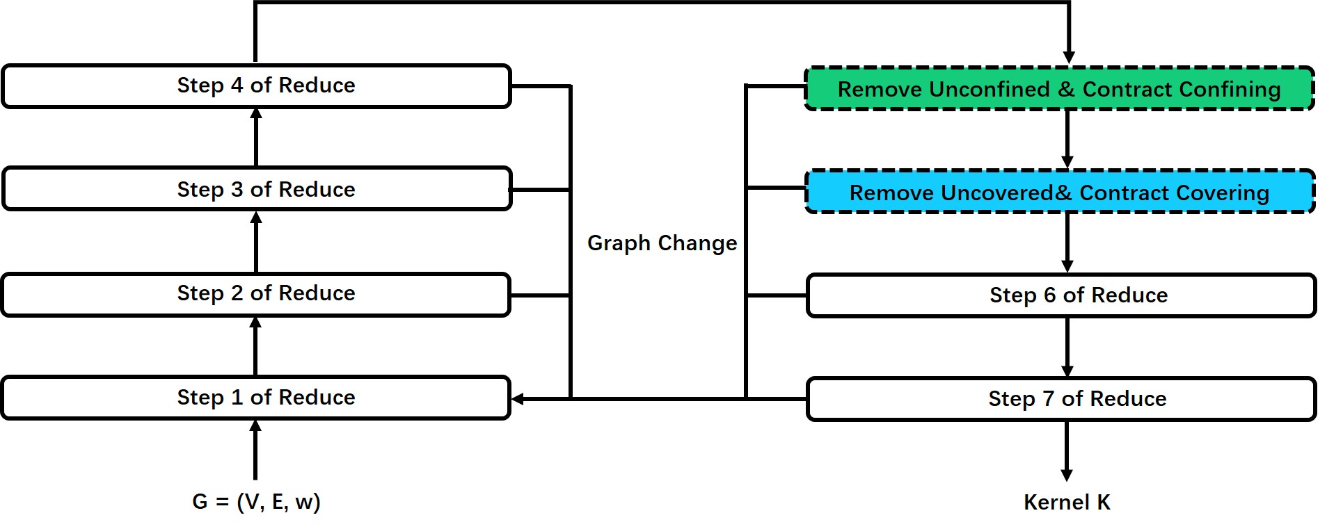
Figure 4: Casual Reduce: Given an input graph $G$, each step of the algorithm is executed sequentially and the graph changes, immediately go back to the first step. When all steps are completed and the graph no longer changes, return to the remaining graph kernel.

Thus, a new reduction algorithm called Causal Reduce can be obtained by using Remove Unconfined & Contract Confining to replace step $5$ of Reduce and adding Remove Uncovered & Contract Covering between Remove Unconfined & Contract Confining and step $6$ of Reduce, which is shown in Figure 4. We will use Causal Reduce$(G)=(K,c)$ to represent the processing of this algorithm on a given input graph $G$. The processing result of this algorithm consists of two parts: One is the remaining graph called kernel $K$ and the other is the weight of the vertex set contained in the MWIS obtained by inference. It’s worth noting that the reduction algorithm Causal Reduce may not resolve all instances directly, but it can be used as a preprocessing for heuristic and exact algorithm.

4.2 The Causal B&R Solver

Before introducing how to integrate our CITs into B&R algorithm, we briefly introduce the state-of-the-art exact algorithm Solve proposed by [27]. Solve is based on the idea of B&R algorithm, which first apply reduction algorithm Reduce to reduce the instance. Then, apply branching rule by virtue of the property of the confining set and perform reduction algorithm Reduce in every branch of the search tree to find a solution. During the searching, it uses a standard technique based on finding upper and lower bounds to prune the search tree and take the best solution weight $W_{b}$ currently found in the algorithm as the lower bound. Initially, let $W_{b}$ be the weight of the solution obtained by heuristic algorithm on the kernel $K$, and update $W_{b}$ once a better solution is obtained in the algorithm. The heuristic algorithm, denoted by Greedy($G$), is a greedy algorithm that iteratively selects a vertex in order of some measure and removes its closed neighbor set from the graph. In each searching branch, it uses a heuristic method to find an upper bound $W_{ub}$ of the optimal solution weight of the current graph, which is based on weight clique covers and is denoted by UpperBound($G$). If the current best solution weight $W_{b}$ is not smaller than $W_{ub}$, then there is no better solution in this searching branch and it can be discarded directly.

Algorithm 1 The Causal B&R Solver($G$)

0:  A vertex weight graph $G=(V,E,w)$;

0:  The weight of a MWIS of $G$.

1:  Initialization of global variable $W_{b}$: $W_{b}\leftarrow 0$;

2:  if weight packing constraints have been created then

3:     while True do

4:        $(K,c)\leftarrow\textbf{Causal Reduce}(G)$;

5:        check constraints();

6:        if existence constraints are not satisfied then

7:           return $W_{b}$;

8:        else if graph is simplified then

9:           continue;

10:        else

11:           break;

12:  else

13:     $(K,c)\leftarrow\textbf{Causal Reduce}(G)$;

14:  $W_{b}\leftarrow\max\{W_{b},c+\textbf{Greedy}(K)\}$;

15:  if $c+\textbf{UpperBound}(G)\leqslant W_{b}$ then

16:     return $W_{b}$;

17:  Pick up a vertex $v$ of maximum degree and compute the confining set $S_{v}$ and the inferred covering set $IC_{v}$;

18:  create weight packing constraint (3.1) and $W_{b}\leftarrow\max\{W_{b},c+w(S_{v})+\textbf{Causal B\&R Solver}(K-N[S_{v}])\}$;

19:  create weight packing constraint (3.2) and $W_{b}\leftarrow\max\{W_{b},c+\textbf{Causal B\&R Solver}(K-IC_{v})\}$;

20:  return $W_{b}$;

Our CITs will be integrated into two parts of Solve, resulting in a new exact algorithm called Causal B&R Solver. The first part is that we will use our reduction algorithm Causal Reduce to reduce the instance to get the kernel $K$, and perform the reduction algorithm on each branch of the search tree. The second part is that we will make use of the state-preserving results of two types of CITs during the branching process. Similar to the idea of Solve in [27], using property of confining set to the branching process, when choosing a vertex with the maximum degree to branch, the state-preserving results of $(b)$ of Corollary 3.11 and $(b)$ of Corollary 3.3 will be used in this part. This means that during branching, we either remove the inferred covering set of the branching vertex from the graph or include the confining set of the branching vertex into the independent set. Furthermore, we will create weight packing constraint (3.2) while removing the inferred covering set of branching vertex. Similarly, we will also create weight packing constraint (3.1) when including the confining set of branching vertex into the independent set. We will keep and manage these weight packing constraints when searching for solutions in each branch of the search tree. Specifically, another step called check constraints is added after the last step of Casual Reduce. In this step, for each weight packing constraint, we will check whether the constraint holds and whether the graph can be simplified by the causal inference properties of that constraint. If any constraint is violated, the searching branch will be skipped. If the graph can be simplified, Causal Reduce will continue to execute after reducing the graph. If none of the above conditions are met, the subsequent process will be performed. The main steps of Causal B&R Solver are listed in Algorithm 1.

4.3 The Causal Search

After taking our reduction algorithm Causal Reduce as a preprocessing, we apply the state-preserving result of second type of CIT to the local search process of heuristic algorithm DynWVC2 [6] to solve the complementary problem of the MWIS problem—the MWVC problem, which leads to a new algorithm called Causal Search.

Algorithm 2 The basic framework of DynWVC2 algorithm.

0:  A vertex weight graph $G=(V,E,w)$, the cutoff time of the running $T$;

0:  A vertex cover of $G$.

1:  $VC\leftarrow$ Construct();

2:  $VC^{*}\leftarrow VC$;

3:  while $elapsed\_time\textless T$ do

4:     $R\leftarrow$ RemoveVertices(VC)

5:     while some edge is uncovered by $VC$ do

6:        choose a vertex $v$ from $N(R)$;

7:        $VC\leftarrow VC\cup\{v\}$;

8:     remove redundant vertices from $VC$;

9:     if $w(VC)\textless w(VC^{*})$ then

10:        $VC^{*}\leftarrow VC$

The DynWVC2 algorithm proposed by [6], is the state-of-the-art heuristic algorithm for solving MWVC problem. The basic framework of this algorithm is shown in Algorithm 2. The local search process of this algorithm mainly consists of a removing phase and an adding phase, and the specific process can be found in [6].

Our CITs will be considered in the removing phase of the algorithm — RemoveVertices function. In this function, there are two scoring functions $loss$ and $valid\_score$ used to select the vertices to remove from the vertex cover $VC$. The specific definition of these two scoring functions can be seen in [6]. The $loss$ and $valid\_score$ functions have fundamentally different effects on the behavior of the algorithm. Vertex selection using $loss$ function is an “exploratory” selection; in other words, it is quite possible that such a chosen vertex is good for the quality of the solution, but this cannot be determined. Different from “exploratory” vertex selection, $valid\_score$ is a “deterministic” selection, that is, we can determine whether removing a vertex will have a positive impact on the quality of the solution. For example, if a vertex has a negative $valid\_score$ value, this means that after removing this vertex and adding its adjacent uncovering vertices, a vertex cover with lower weight than the current vertex cover can be obtained [6].

In removing phase, the vertex with the minimum loss is removed from vertex cover $VC$ first, and then the second removed vertex is selected by a dynamic vertex selection strategy. The details of dynamic vertex selection strategy can be learned in [6]. After removing the two vertices, if the total degree of the removed vertices does not reach a predetermined value (which is set to $2$ times average degree of the graph), another vertex to be selected with the BMS strategy [5], which samples $t$ ($t=50$) vertices from vertex cover $VC$ and chooses the one with the minimum $loss$, will be removed to expand the search region. In this way, it solves the problem that when removing two vertices the resulting search area is too small and limits the ability of the adding phase to find better local optima. If the search area obtained by removing two vertices is large enough, in order to balance the search time and search quality, the third vertex will not be selected for removing.

The state-preserving result of second type of CIT will be applied to the dynamic vertex selection strategy for selecting the second vertex to be removed. The dynamic vertex selection strategy consists of a primary vertex scoring function $valid\_score$ and a secondary scoring function $loss$. When the removed vertex $v$ is selected by $valid\_score$ function, it can be seen from the nature of the $valid\_score$ function: There is a high probability that there exists a MWIS $I$ containing it. If the vertex $v$ is indeed included in $I$, by $(a)$ of Corollary 3.11, the corresponding inferred confining set $IS_{v}$ also contained in $I$. Inspired by this result, when selecting the second removed vertex $v$ by scoring function $valid\_score$, we will remove the vertices in the inferred confining set $IS_{v}$ from the vertex cover $VC$. In this way, the search region can be expanded and the number of times to continue to use the third removed vertex to expand the search area is reduced, which means that the ability of local search to find better local optima is improved. An example of our CITs applied to the vertex removing process is presented in Figure 5.

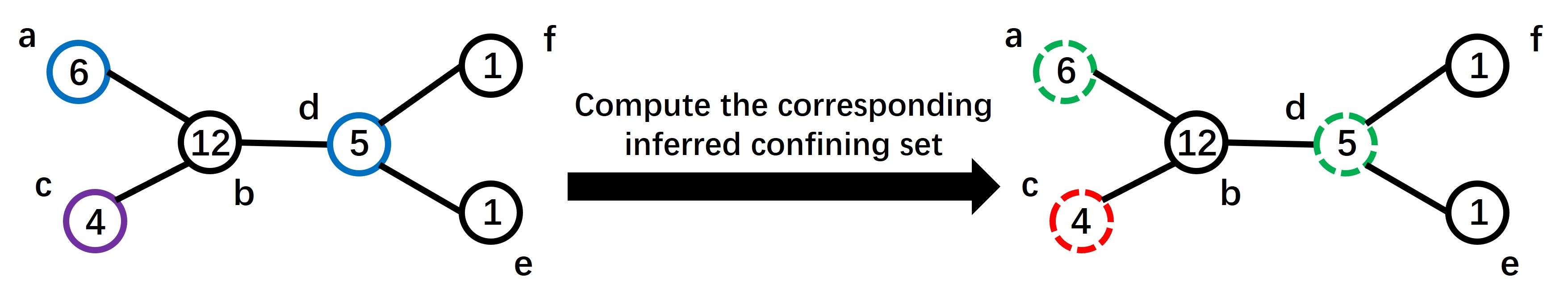
Figure 5: Example of our CITs applied to the vertex removing process: When we utilize $valid\_score$ to select the removed vertex $c$ from the vertex cover $VC=\{a,c,d\}$, we can compute the corresponding inferred confining set $IS_{c}=\{a,c,d\}$ of vertex $c$ and remove set $IS_{c}$ from vertex cover $VC$.

In addition, it can be seen from the calculation process of Definition 3.9 about the inferred confining set: the computational complexity of $IS_{v}$ for each vertex $v$ is $O(|N(IS_{v})||IS_{v}|)$. This means that in the actual application process, since the size of the generally obtained inferred confining set is relatively small, its computational cost is very small. Thus, our CITs is helpful for improving the performance of local search process.

5 Experiments

We will conduct four experiments to verify the effect of integrating our CITs into current algorithmic frameworks. The first experiment is used to analyze the impact of our CITs for the reduction algorithm. The examination of the performance gain of our CITs in the B&R algorithm is shown in the second experiment. The third experiment is used to test the ability of our Causal Reduce as a preprocessing to improve the performance of the heuristic algorithm. The last experiment is conducted to verify the effect of adding our CITs to the local search process of heuristic algorithm.

Experiment environment Setup. All of our algorithms are implemented in C++, and compiled by g++ with ‘-O3’ option. All experiments are run on a platform with $128$G RAM and one Intel(R) Xeon(R) Gold $5117$ CPU @ $2.00$GHz.

Compared Algorithms. In previous studies, most of them only use some simple rules as preprocessing to reduce problem instances, and do not pay attention to the performance of preprocessing. Two recent papers [15, 27] have studied in depth the reduction rules for the MWIS and analyzed their performance. Since the algorithm Reduce in [27] outperforms the algorithm in [15] and our Causal Reduce is obtained by integrating our CITs into Reduce, in this paper, we only use it as a baseline to analyze the impact of our CITs for the reduction algorithm. Additionally, in order to fully understand the role of different CITs on the reduction algorithm, we control the application of CITs in Reduce and conduct comparative experiments. Similar to the Causal Reduce shown in Figure 4, we use Re-Confin to represent the algorithm obtained after replacing the step $5$ of Reduce with Remove Unconfined & Contract Confining and Re-Cover to denote the algorithm obtained by adding Remove Uncovered & Contract Covering between step $5$ and $6$ of Reduce.

On the basis of the reduction algorithm Reduce, the authors of [27] also developed a fast exact algorithm Solve, which is the state-of-art exact algorithm in previous work, and our Causal B&R Solver is obtained by applying our CITs into it, so it will be used as a baseline to verify the performance improvement of our CITs for the B&R algorithm. Furthermore, we use Solve-CR to identify the algorithm obtained by replacing Reduce with Causal Reduce in Solve, Solve-CR-IC refers to the algorithm obtained by further simplifying the branch by using the inferred covering set of the branching vertex in the branching process on the basis of Solve-CR, and Solve-Packing to represent the algorithm obtained by applying our weight packing constraints to the branching process of Solve. We will conduct comparative experiments on these algorithms to clarify the impact of different CITs on the B&R algorithm.

Two state-of-the-art heuristic algorithms FastWVC (Fast) [7] and DynWVC2 (Dyn) [6] will be used to verify that our Causal Reduce as preprocessing improves the performance of the heuristic algorithm. We will use Causal Re + Fast and Causal Re + Dyn to denote applying our Causal Reduce as preprocessing before executing FastWVC and DynWVC2. In addition, to further verify the superiority of our Causal Reduce as preprocessing for improving the performance of the heuristic algorithm, we also conduct comparative experiments using Reduce as a preprocessing of the heuristic algorithm. Likewise, we use Re + Fast and Re + Dyn to indicate the application of the previous reduction algorithm Reduce before FastWVC and DynWVC2 are executed. Moreover, our Causal Search is obtained by integrating CITs into the local search process of DynWVC2. Therefore, we can verify the effect of this operation by comparing DynWVC2 with Causal Search.

Instances. We evaluate all algorithms on six real graphs which are most representative and most difficult graphs from different domains. These graphs are downloaded from Network Data Repository [21]. All of them have $100$ thousands to millions of vertices, and dozens of millions of edges. These instances become popular in recent works for the MWIS problem. Statistics of these graphs are shown in Table 2. In our experiment, the weight of each vertex in the graph will have two random allocation mechanisms , which are commonly used in previous work [15, 27, 6, 7]. The first allocation mechanism is that the weight of each vertex in the graph is obtained from $[1,200]$ uniformly at random, we will number the six datasets with $1-6$. The second allocation mechanism is that the weight of each vertex in the graph follows a random uniform distribution of $[20,100]$, and $7-12$ will be used to number the six datasets.

	inf-road-usa	soc-livejournal	sc-ldoor	tech-as-skitter	sc-msdoor	inf-roadNet-CA
Vertices	$23947347$	$4033137$	$952203$	$1694616$	$415863$	$1957027$
Edges	$28854312$	$27933062$	$20770807$	$11094209$	$9378650$	$2760388$
NO.	$1$, $7$	$2$, $8$	$3$, $9$	$4$, $10$	$5$, $11$	$6$, $12$

Table 2: All graphs are sorted in descending order regarding the number of edges. In the row headed by “NO.”, each number is used to represent the corresponding number of the dataset generated by the graph according to the corresponding vertex weight allocation mechanism.

5.1 Impact of CITs on Reduction Algorithm

We first analyze the impact of our CITs for the reduction algorithm and evaluate the performance of all reduction algorithms by measuring the running time, the size of the remaining graphs (kernel size), and the ratio of the kernel size to the number of vertices in the original graph (We simply refer to it here as the ratio for convenience.).

		Reduce			Re-Confin			Re-Cover			Causal Reduce
NO.	$|V|$	Time(S)	Kernel Size	Ratio(%)	Time(S)	Kernel Size	Ratio(%)	Time(S)	Kernel Size	Ratio(%)	Time(S)	Kernel Size	Ratio(%)
$\mathbf{1}$	$23947347$	$72.00$	$431891$	$1.80$	$71.66$	$428137$	$1.79$	$74.03$	$431888$	$1.80$	$\underline{55.88}$	$\bf 275082$	$1.15$
$\mathbf{2}$	$4033137$	$\underline{12.93}$	$7273$	$0.18$	$16.57$	$5960$	$0.15$	$16.20$	$7261$	$0.18$	$17.92$	$\bf 3281$	$0.08$
$\mathbf{3}$	$952203$	$\underline{3.08}$	$6492$	$0.68$	$3.89$	$2780$	$0.29$	$3.89$	$6447$	$0.68$	$3.84$	$\bf 1682$	$0.18$
$\mathbf{4}$	$1694616$	$\underline{1.78}$	$5904$	$0.35$	$2.32$	$5613$	$0.33$	$2.26$	$5909$	$0.35$	$5.03$	$\bf 3974$	$0.23$
$\mathbf{5}$	$415863$	$\underline{1.66}$	$6570$	$1.58$	$1.84$	$3166$	$0.76$	$2.04$	$6570$	$1.58$	$1.86$	$\bf 2162$	$0.52$
$\mathbf{6}$	$1957027$	$76.14$	$305470$	$15.61$	$63.65$	$300135$	$15.34$	$76.57$	$305470$	$15.61$	$\underline{41.12}$	$\bf 202885$	$10.37$
$\mathbf{7}$	$23947347$	$117.54$	$437993$	$1.83$	$94.52$	$434606$	$1.81$	$113.07$	$438004$	$1.83$	$\underline{58.02}$	$\bf 235243$	$0.98$
$\mathbf{8}$	$4033137$	$\underline{11.68}$	$7620$	$0.19$	$15.90$	$6371$	$0.16$	$15.65$	$7576$	$0.19$	$23.38$	$\bf 3806$	$0.09$
$\mathbf{9}$	$952203$	$8.05$	$29116$	$3.06$	$5.08$	$7906$	$0.83$	$8.88$	$29116$	$3.06$	$\underline{5.06}$	$\bf 4628$	$0.49$
$\mathbf{10}$	$1694616$	$\underline{1.94}$	$6999$	$0.41$	$2.55$	$6623$	$0.39$	$2.53$	$6991$	$0.41$	$5.19$	$\bf 4429$	$0.26$
$\mathbf{11}$	$415863$	$4.09$	$24736$	$5.95$	$2.75$	$10098$	$2.43$	$4.24$	$24736$	$5.95$	$\underline{2.66}$	$\bf 7081$	$1.70$
$\mathbf{12}$	$1957027$	$19.01$	$131498$	$6.72$	$17.00$	$128637$	$6.57$	$19.54$	$131498$	$6.72$	$\underline{8.64}$	$\bf 65124$	$3.33$

Table 3: Impact of CITs for the the reduction algorithm. The bold and underlined numbers are the minimum kernel size and shortest running time, respectively.

The experimental results of all algorithms are output in Table 3. We can know that all reduction algorithms can significantly simplify the graph, and even reduce the graph to less than $0.1\%$ of the original size. Besides, we can see that our Causal Reduce achieves best reduction effect in all datasets, that is, our Causal Reduce results in a much smaller kernel size than other algorithms. Moreover, compared with Reduce, Re-Confin can achieve better reduction effect in all datasets, while Re-Cover has basically no performance improvement. This shows that replacing the step $5$ of Reduce with Remove Unconfined & Contract Confining plays a key role in improving the performance of the reduction algorithm, and combined with Remove Uncovered & Contract Covering, the performance of the reduction algorithm will be greatly improved, but only adding Remove Uncovered & Contract Covering can hardly improve the performance of the reduction algorithm.

More notably, our Causal Reduce take less time than other algorithms on half of the datasets. On the rest of the datasets, our Causal Reduce only takes a few seconds longer than other algorithms. These phenomena show that integrating our CITs into the reduction algorithm can significantly improve the performance of the algorithm, but the increase in time cost is very small, and they can even reduce the time cost.

5.2 Performance Gain of CITs on the B&R Algorithm

We will examine the performance gain of our CITs for B&R algorithm. The running time bound is set as $1,000$ seconds for all algorithms, and if the algorithm cannot find the optimal solution within the time bound, the best solution found in all search branches is output.

	Solve		Solve-CR		Solve-Packing		Solve-CR-IC		Causal B&R Solver
NO.	Time(S)	Result	Time(S)	Result	Time(S)	Result	Time(S)	Result	Time(S)	Result
$\mathbf{1}$	$1000$	$1380579565$	$1000$	$1380810330$	$1000$	$1380579506$	$1000$	$1380980673$	$1000$	$\bf 1380980749$
$\mathbf{2}$	$1000$	$232813323$	$28.5058$	$\bf 232828253$	$1000$	$232814520$	$28.8413$	$\bf 232828253$	$\underline{25.4889}$	$\bf 232828253$
$\mathbf{3}$	$\underline{3.8108}$	$\bf 10303506$	$5.3508$	$\bf 10303506$	$4.7170$	$\bf 10303506$	$4.1507$	$\bf 10303506$	$3.9148$	$\bf 10303506$
$\mathbf{4}$	$1000$	$124020452$	$1000$	$124020466$	$1000$	$124020706$	$1000$	$124021474$	$1000$	$\bf 124022398$
$\mathbf{5}$	$1000$	$3904552$	$\underline{4.2820}$	$\bf 3916599$	$1000$	$3904544$	$4.3919$	$\bf 3916599$	$4.33729$	$\bf 3916599$
$\mathbf{6}$	$1000$	$100956490$	$1000$	$101259145$	$1000$	$100957090$	$1000$	$101259161$	$1000$	$\bf 101288073$
$\mathbf{7}$	$1000$	$798872105$	$1000$	$799021102$	$1000$	$798911163$	$1000$	$\bf 799021209$	$1000$	$\bf 799021209$
$\mathbf{8}$	$1000$	$134613130$	$34.0139$	$\bf 134621271$	$1000$	$134613130$	$34.4151$	$\bf 134621271$	$\underline{32.1868}$	$\bf 134621271$
$\mathbf{9}$	$1000$	$7237240$	$\underline{6.8162}$	$\bf 7273973$	$1000$	$7237411$	$6.8372$	$\bf 7273973$	$6.9285$	$\bf 7273973$
$\mathbf{10}$	$1000$	$71945454$	$1000$	$71944343$	$1000$	$\bf 71946049$	$1000$	$71944343$	$1000$	$71945241$
$\mathbf{11}$	$1000$	$2707746$	$1000$	$\bf 2743962$	$1000$	$2707846$	$1000$	$\bf 2743962$	$1000$	$\bf 2743962$
$\mathbf{12}$	$1000$	$61702804$	$1000$	$61818326$	$1000$	$61702794$	$1000$	$\bf 61819495$	$1000$	$61818234$

Table 4: Performance gain of CITs on B&R algorithm. The bold and underlined numbers are the best numerical results of all algorithms and the shortest running time of all algorithms to find the optimal solution, respectively.

We output the numerical results and running times of all algorithms in Table 4. It can be seen from Table 4 that Solve-CR and Solve-CR-IC, like our Causal B&R Solver, can obtain the optimal solution in five data sets, while Solve-Packing, like Solve, can only obtain the optimal solution in one data set. In addition, on those datasets where the optimal solution cannot be solved within $1000$ seconds, our Causal B&R Solver can basically obtain better numerical solutions than Solve-CR-IC, and Solve-CR-IC can obtain numerical results that are slightly better than Solve-CR, while Solve-Packing can generally get better numerical solutions than Solve. These results demonstrate that our reduction algorithm, Causal Reduce, is critical for the B&R algorithm to obtain optimal solutions on more datasets. Moreover, both the inferred covering set of the branching vertex and the weighted packing constraints can help B&R algorithm find more promising branches and find better solutions.

5.3 Causal Reduce’s Improvement on Heuristic Algorithm

Next, we will verify the superiority of our Causal Reduce as a preprocessing for improving the heuristic algorithm. Table 5 presents the running time (including preprocessing time) and numerical results. We find that the preprocessed heuristic algorithm with Causal Reduce usually stop execution after running for a short time, while the rest of the heuristic algorithms are allowed to run for $1000$ seconds. Meanwhile, it can be observed from Table 5 that adding the reduction algorithm as preprocessing is obvious for improving the performance of the heuristic algorithm, and our Causal Reduce helps heuristics find better solutions on all instances in less time (essentially within 100 seconds) than Reduce. Thus, although our Causal Reduce takes no more than $12$ seconds longer than Reduce on half of the datasets (as can be known from the numerical results in Section 5.1), it can further reduce the size of remaining graph by more than $32.6\%$, which is critical for subsequent processing of the problem (also be mentioned in Section 5.2), so such processing time cost is worth it!

	Fast		Re + Fast		Causal Re + Fast		Dyn		Re + Dyn		Causal Re + Dyn
NO.	Time(S)	Result	Time(S)	Result	Time(S)	Result	Time(S)	Result	Time(S)	Result	Time(S)	Result
$\mathbf{1}$	$1000$	$1308864893$	$1000$	$1381212394$	$\underline{250}$	$\bf 1381215439$	$1000$	$1310465732$	$1000$	$1381174854$	$\underline{100}$	$\bf 1381178355$
$\mathbf{2}$	$1000$	$227121250$	$1000$	$232826881$	$\underline{20}$	$\bf 232827816$	$1000$	$229769205$	$1000$	$232827891$	$\underline{20}$	$\bf 232828157$
$\mathbf{3}$	$1000$	$10044429$	$1000$	$10302725$	$\underline{5}$	$\bf 10303465$	$1000$	$10224463$	$1000$	$10303168$	$\underline{5}$	$\bf 10303476$
$\mathbf{4}$	$1000$	$122468973$	$1000$	$124025600$	$\underline{6}$	$\bf 124026219$	$1000$	$123179849$	$1000$	$124026286$	$\underline{6}$	$\bf 124026433$
$\mathbf{5}$	$1000$	$3823908$	$1000$	$3916222$	$\underline{3}$	$\bf 3916534$	$1000$	$3894401$	$1000$	$3916381$	$\underline{3}$	$\bf 3916568$
$\mathbf{6}$	$1000$	$97155884$	$1000$	$101739247$	$\underline{275}$	$\bf 101745579$	$1000$	$99122831$	$1000$	$101740261$	$\underline{250}$	$\bf 101744463$
$\mathbf{7}$	$1000$	$756581612$	$1000$	$799087671$	$\underline{150}$	$\bf 799111311$	$1000$	$757212666$	$1000$	$799058579$	$\underline{70}$	$\bf 799083159$
$\mathbf{8}$	$1000$	$131848587$	$1000$	$134620719$	$\underline{25}$	$\bf 134621064$	$1000$	$132970128$	$1000$	$134621142$	$\underline{25}$	$\bf 134621249$
$\mathbf{9}$	$1000$	$7131770$	$1000$	$7273626$	$\underline{6}$	$\bf 7273655$	$1000$	$7252153$	$1000$	$7273750$	$\underline{6}$	$\bf 7273931$
$\mathbf{10}$	$1000$	$70966490$	$1000$	$71946839$	$\underline{6}$	$\bf 71947488$	$1000$	$71459210$	$1000$	$71947516$	$\underline{6}$	$\bf 71947590$
$\mathbf{11}$	$1000$	$2682982$	$1000$	$2748925$	$\underline{25}$	$\bf 2748945$	$1000$	$2743648$	$1000$	$2748982$	$\underline{10}$	$\bf 2749005$
$\mathbf{12}$	$1000$	$59619787$	$1000$	$61850413$	$\underline{50}$	$\bf 61852628$	$1000$	$60802433$	$1000$	$61855209$	$\underline{75}$	$\bf 61857313$

Table 5: A comparative experiment of the effect of Causal Reduce on improving the heuristic algorithm. The numbers in bold and underlined are the corresponding experimental results and running time (including preprocessing time) of each heuristic algorithm using our Causal Reduce as preprocessing, respectively.

5.4 Comparative Experiment on Causal Search

On the basis of preprocessing the input graph with Causal Reduce, we will compare our Causal Search with DynWVC2 to verify the effect of adding CITs to the local search process of DynWVC2 algorithm. The running time for both algorithms (including pre-processing time) is set to $1000$ seconds. To avoid randomness, we run each instance $5$ times and record the mean and maximum values. Furthermore, in order to estimate the gap between the results obtained by these two algorithms and the MWIS, we need to calculate the upper bound of each instance. The upper bound for the $2$nd, $3$rd, $5$th, $8$th, $9$th instance is nothing but the weight of the optimal solution obtained by Causal B&R Solver, and for the rest of the instances, it is obtained by applying the weighted clique cover method mentioned in Section 4.2 to the remaining graph obtained by Causal Reduce. Table 6 outputs the numerical results and the estimated gap. The small gaps there demonstrate that after preprocessing with our Causal Reduce, both algorithms can obtain numerical results very close to the optimal solution. In particular, for those instances where the optimal solution is obtained, their gap can basically reach $10^{-6}\sim 10^{-7}$, and in the remaining instances, the estimated gap can basically reach $10^{-4}\sim 10^{-2}$. Besides, from the mean and maximum values, our Causal Search can basically achieve better performance than DynWVC2, thereby implying that our CITs can help local search find better local optima.

		Dyn				Causal Search
NO.	Upper Bound	Mean	Gap	Max	Gap	Mean	Gap	Max	Gap
$\mathbf{1}$	$1384376268$	$1381464698.6$	$2.103\times 10^{-3}$	$1381467306$	$2.101\times 10^{-3}$	$\underline{1381466033.6}$	$2.102\times 10^{-3}$	$\bf 1381470750$	$2.099\times 10^{-3}$
$\mathbf{2}$	$232828253$	$232828153.4$	$4.278\times 10^{-7}$	$232828171$	$3.522\times 10^{-7}$	$\underline{232828159.2}$	$4.029\times 10^{-7}$	$\bf 232828188$	$2.792\times 10^{-7}$
$\mathbf{3}$	$10303506$	$10303485.2$	$2.019\times 10^{-6}$	$10303491$	$1.456\times 10^{-6}$	$\underline{10303488.6}$	$1.689\times 10^{-6}$	$\bf 10303494$	$1.165\times 10^{-6}$
$\mathbf{4}$	$124076790$	$124026438.6$	$4.058\times 10^{-4}$	$\bf 124026451$	$4.057\times 10^{-4}$	$\underline{124026444.8}$	$4.058\times 10^{-4}$	$124026449$	$4.057\times 10^{-4}$
$\mathbf{5}$	$3916599$	$3916582.2$	$4.289\times 10^{-6}$	$3916583$	$4.085\times 10^{-6}$	$\underline{3916582.6}$	$4.187\times 10^{-6}$	$\bf 3916584$	$3.830\times 10^{-6}$
$\mathbf{6}$	$103562461$	$101846521.0$	$1.657\times 10^{-2}$	$101848242$	$1.655\times 10^{-2}$	$\underline{101847524.8}$	$1.656\times 10^{-2}$	$\bf 101849650$	$1.654\times 10^{-2}$
$\mathbf{7}$	$800748442$	$799264479.2$	$1.853\times 10^{-3}$	$799265827$	$1.852\times 10^{-3}$	$\underline{799266278.8}$	$1.851\times 10^{-3}$	$\bf 799267573$	$1.849\times 10^{-3}$
$\mathbf{8}$	$134621271$	$134621255.0$	$1.189\times 10^{-7}$	$134621257$	$1.040\times 10^{-7}$	$\underline{134621256.8}$	$1.055\times 10^{-7}$	$\bf 134621265$	$4.457\times 10^{-6}$
$\mathbf{9}$	$7273973$	$\underline{7273939.8}$	$4.564\times 10^{-6}$	$7273945$	$3.849\times 10^{-6}$	$7273936.8$	$4.977\times 10^{-6}$	$\bf 7273947$	$3.574\times 10^{-6}$
$\mathbf{10}$	$71978922$	$71947636.0$	$4.347\times 10^{-4}$	$71947639$	$4.346\times 10^{-4}$	$\underline{71947636.8}$	$4.346\times 10^{-4}$	$\bf 71947642$	$4.346\times 10^{-4}$
$\mathbf{11}$	$2819343$	$2749008.4$	$2.495\times 10^{-2}$	$2749009$	$2.495\times 10^{-2}$	$\underline{2749010.8}$	$2.495\times 10^{-2}$	$\bf 2749019$	$2.494\times 10^{-2}$
$\mathbf{12}$	$62276875$	$61860510.4$	$6.686\times 10^{-3}$	$61860616$	$6.684\times 10^{-3}$	$\underline{61860549.0}$	$6.685\times 10^{-3}$	$\bf 61860717$	$6.682\times 10^{-3}$

Table 6: Compare our Causal Search with the DynWVC2 algorithm. The bold and underlined numbers are better maximum and average values, respectively. In the column headed by “Upper Bound”, each number is the upper bound of the MWIS of the corresponding instance.

6 Conclusion and Outlook

In this paper, we propose a series of causal inference techniques (CITs) for the maximum weight independent set (MWIS) problem by fully exploiting the upper bound property of MWIS. After integrating our CITs, the performance of various existing algorithms, including the Branch-and-Reduce (B&R) algorithm and some heuristic algorithms, is significantly improved. We are now conducting theoretical analysis to find some guarantees on solution quality, developing strategies to help the B&R algorithm analyze the causes of conflicts and perform more efficient backtracking searches, and generalizing the proposed CITs to other combinatorial optimization problems.

References

- [1] T. Akiba and Y. Iwata, Branch-and-reduce exponential/fpt algorithms in practice: A case study of vertex cover, Theoretical Computer Science, 609 (2016), pp. 211–225.
- [2] A. Avenali, Resolution branch and bound and an application: the maximum weighted stable set problem, Operations research, 55 (2007), pp. 932–948.
- [3] L. Babel, A fast algorithm for the maximum weight clique problem, Computing, 52 (1994), pp. 31–38.
- [4] E. Balas and C. S. Yu, Finding a maximum clique in an arbitrary graph, SIAM Journal on Computing, 15 (1986), pp. 1054–1068.
- [5] S. Cai, Balance between complexity and quality: Local search for minimum vertex cover in massive graphs, in Twenty-Fourth International Joint Conference on Artificial Intelligence, 2015, pp. 747–753.
- [6] S. Cai, W. Hou, J. Lin, and Y. Li, Improving local search for minimum weight vertex cover by dynamic strategies., in Twenty-Seventh International Joint Conference on Artificial Intelligence, 2018, pp. 1412–1418.
- [7] S. Cai, Y. Li, W. Hou, and H. Wang, Towards faster local search for minimum weight vertex cover on massive graphs, Information Sciences, 471 (2019), pp. 64–79.
- [8] L. Chang, W. Li, and W. Zhang, Computing a near-maximum independent set in linear time by reducing-peeling, in Proceedings of the 2017 ACM International Conference on Management of Data, 2017, pp. 1181–1196.
- [9] S. Coniglio and S. Gualandi, Optimizing over the closure of rank inequalities with a small right-hand side for the maximum stable set problem via bilevel programming, INFORMS Journal on Computing, 34 (2022), pp. 1006–1023.
- [10] J. Dahlum, S. Lamm, P. Sanders, C. Schulz, D. Strash, and R. F. Werneck, Accelerating local search for the maximum independent set problem, in International symposium on experimental algorithms, 2016, pp. 118–133.
- [11] M. A. Dzulfikar, J. K. Fichte, and M. Hecher, The pace 2019 parameterized algorithms and computational experiments challenge: The fourth iteration, in 14th International Symposium on Parameterized and Exact Computation, vol. 148, 2019, pp. 25:1–25:23.
- [12] T. A. Feo, M. G. Resende, and S. H. Smith, A greedy randomized adaptive search procedure for maximum independent set, Operations Research, 42 (1994), pp. 860–878.
- [13] F. V. Fomin, F. Grandoni, and D. Kratsch, A measure & conquer approach for the analysis of exact algorithms, Journal of the ACM, 56 (2009), pp. 1–32.
- [14] J. Kneis, A. Langer, and P. Rossmanith, A fine-grained analysis of a simple independent set algorithm, in IARCS Annual Conference on Foundations of Software Technology and Theoretical Computer Science, vol. 4, 2009, pp. 287–298.
- [15] S. Lamm, C. Schulz, D. Strash, R. Williger, and H. Zhang, Exactly solving the maximum weight independent set problem on large real-world graphs, in Proceedings of the Twenty-First Workshop on Algorithm Engineering and Experiments, 2019, pp. 144–158.
- [16] C.-M. Li, Z. Fang, H. Jiang, and K. Xu, Incremental upper bound for the maximum clique problem, INFORMS Journal on Computing, 30 (2018), pp. 137–153.
- [17] C.-S. Liao, C.-W. Liang, and S. H. Poon, Approximation algorithms on consistent dynamic map labeling, Theoretical Computer Science, 640 (2016), pp. 84–93.
- [18] B. Nogueira, R. G. Pinheiro, and A. Subramanian, A hybrid iterated local search heuristic for the maximum weight independent set problem, Optimization Letters, 12 (2018), pp. 567–583.
- [19] R. Plachetta and A. van der Grinten, Sat-and-reduce for vertex cover: Accelerating branch-and-reduce by sat solving, in Proceedings of the Workshop on Algorithm Engineering and Experiments, 2021, pp. 169–180.
- [20] W. Pullan, Optimisation of unweighted/weighted maximum independent sets and minimum vertex covers, Discrete Optimization, 6 (2009), pp. 214–219.
- [21] R. Rossi and N. Ahmed, The network data repository with interactive graph analytics and visualization, in Twenty-ninth AAAI conference on artificial intelligence, 2015, pp. 4292–4293.
- [22] P. San Segundo, F. Furini, and J. Artieda, A new branch-and-bound algorithm for the maximum weighted clique problem, Computers Operations Research, 110 (2019), pp. 18–33.
- [23] E. C. Sewell, A branch and bound algorithm for the stability number of a sparse graph, INFORMS Journal on Computing, 10 (1998), pp. 438–447.
- [24] S. J. Shyu, P.-Y. Yin, and B. M. Lin, An ant colony optimization algorithm for the minimum weight vertex cover problem, Annals of Operations Research, 131 (2004), pp. 283–304.
- [25] D. Strash, On the power of simple reductions for the maximum independent set problem, in International Computing and Combinatorics Conference, vol. 9797, Springer, 2016, pp. 345–356.
- [26] J. S. Warren and I. V. Hicks, Combinatorial branch-and-bound for the maximum weight independent set problem, Relatório Técnico, Texas AM University, Citeseer, 9 (2006), p. 17.
- [27] M. Xiao, S. Huang, Y. Zhou, and B. Ding, Efficient reductions and a fast algorithm of maximum weighted independent set, in Proceedings of the Web Conference 2021, 2021, pp. 3930–3940.
- [28] M. Xiao and H. Nagamochi, Confining sets and avoiding bottleneck cases: A simple maximum independent set algorithm in degree-3 graphs, Theoretical Computer Science, 469 (2013), pp. 92–104.
- [29] H. Xu, T. Kumar, and S. Koenig, A new solver for the minimum weighted vertex cover problem, in International Conference on AI and OR Techniques in Constraint Programming for Combinatorial Optimization Problems, vol. 9676, 2016, pp. 392–405.