A Nearly-Linear Time Algorithm for Minimizing Risk of Conflict in Social Networks

Abstract.

Concomitant with the tremendous prevalence of online social media platforms, the interactions among individuals are unprecedentedly enhanced. People are free to interact with acquaintances, express and exchange their own opinions through commenting, liking, retweeting on online social media, leading to resistance, controversy and other important phenomena over controversial social issues, which have been the subject of many recent works. In this paper, we study the problem of minimizing risk of conflict in social networks by modifying the initial opinions of a small number of nodes. We show that the objective function of the combinatorial optimization problem is monotone and supermodular. We then propose a naïve greedy algorithm with a $(1-1/e)$ approximation ratio that solves the problem in cubic time. To overcome the computation challenge for large networks, we further integrate several effective approximation strategies to provide a nearly linear time algorithm with a $(1-1/e-\epsilon)$ approximation ratio for any error parameter $\epsilon>0$. Extensive experiments on various real-world datasets demonstrate both the efficiency and effectiveness of our algorithms. In particular, the fast one scales to large networks with more than two million nodes, and achieves up to $20\times$ speed-up over the state-of-the-art algorithm.

1. Introduction

It has been extensively studied in the social science literature how opinions evolve and shape through social interactions between individuals with potentially differing opinions (DeGroot, 1974; Friedkin and Johnsen, 1990). In the current digital age, the tremendous prevalence of online social networks and social media provide unprecedented access to social interactions, expression and exchange of opinions, leading to fundamental changes of ways people share and formulate opinions. The uninhibited access to information and expression of opinions leads to the emergence or reinforcement of various social phenomena, such as polarization, disagreement, controversy, and resistance, which are signified in (Chen et al., 2018) by the term conflict in a more generic manner. For example, users in the virtual world tend to create connections with like-minded individuals, which separates individuals into groups forming “echo-chambers” or “filter bubbles”. Individuals in different groups have little even no communication with each other, whose opinions do not reach consensus but are opposing, leading to and reinforcing polarization and disagreement.

The identification (Xu et al., 2021), quantification (Chen et al., 2018; Musco et al., 2018), and optimization (Matakos et al., 2017; Musco et al., 2018; Haddadan et al., 2021; Garimella et al., 2017; Bindel et al., 2015; Gaitonde et al., 2020) of conflict are fundamental tasks behind a myriad of high-impact data mining applications, and thus have received considerable attention. Since conflict has a corrosive and detrimental risk to the functioning of communities and societies (Matakos et al., 2017), it is thus of significance to reduce the risk of conflict through some targeted interventions, minimizing or mitigating those negative effects. In this paper, we focus on optimizing two primary measures of conflict, controversy and resistance, with the former also called polarization in (Matakos et al., 2017; Musco et al., 2018). Specifically, we minimize controversy and resistance by changing the opinions of a small number of individuals, which can be achieved by raising awareness and enforcing education of individuals, among other typical strategies or means (Matakos et al., 2017; Musco et al., 2018; Gaitonde et al., 2020).

Shortcomings in the state-of-the-art. The study of optimizing conflict in social media by convincing a small number of people to adopt a different stand is not new. In (Matakos et al., 2017), an algorithm called BOMP was proposed to reduce controversy by selecting a group of $k$ individuals in a social network with $n$ nodes and $m$ edges, and convincing them to change their initial opinions to $0$. The computational complexity of BOMP is $O(kn^{2})$. As an input of algorithm BOMP, the forest matrix (Golender et al., 1981; Chebotarev, 2008) is assumed to have been pre-computed in (Matakos et al., 2017). Actually, the computation of forest matrix involves matrix inverse, which is time-consuming and requires time $O(n^{3})$. To tackle this computation challenge, we develop a nearly linear time algorithm with respect to $m$, the number of edges. In addition, BOMP is designed for minimizing controversy, while our approach is also applicable to the optimization of resistance.

Contributions. In this paper, we address the following optimization problem: given a social network with $n$ nodes and $m$ edges, a vector $\bm{\mathit{s}}$ of initial opinions, and a budget value $k$, how to strategically identify $k$ nodes and change their initial opinions to zero, in order to minimize two conflict measures, controversy and resistance. Our main contributions include the following three aspects. First, we unify the two optimization objectives into one framework, and show that the unified objective function is supermodular and monotone. Then, based on the obtained properties of the objective function, we propose two greedy algorithms, Greedy and Greedy-AC, to solve the problem. Greedy has a $(1-1/e)$ approximation ratio with computation complexity of $O(n^{3})$, while Greedy-AC has a $(1-1/e-\epsilon)$ approximation ratio with computation complexity $\widetilde{O}(mk\epsilon^{-2})$ for any $\epsilon>0$, where $\epsilon>0$ is the error parameter and the $\widetilde{O}(\cdot)$ notation suppresses the ${\rm poly}(\log n)$ factors. Finally, we evaluate the performance of our algorithms by executing extensive experiments on various real-world networks, which show that Greedy-AC is as effective as Greedy and BOMP, all of which outperform several baseline strategies. Moreover, Greedy-AC is more efficient than Greedy and BOMP, with Greedy-AC achieving up to $20\times$ speed-up over Greedy and BOMP on moderately sized networks with $24$ thousand nodes. In particular, Greedy-AC is scalable to large networks with more than two million nodes.

2. Related work

In this section, we briefly review the related literature.

Optimization of polarization and controversy. Due to the negative effects of polarization and controversy, a lot of works have been devoted to designing strategies to decrease these two correlated quantities. For instance, in (Haddadan et al., 2021) and (Garimella et al., 2017), link addition was considered to maximally reduce the polarized bubble radius and controversy, respectively. Both of these two existing works focus on graph-theoretic measures of polarization or controversy, which do not take the initial opinions of individuals into consideration. Furthermore, both of them exploit the strategy of the link addition to achieve the goal, instead of the modification of initial opinions.

The closest to our work lies that of (Musco et al., 2018) and (Matakos et al., 2017). In (Musco et al., 2018), the $\ell_{2}$ norm of $\overline{\bm{\mathit{z}}}=\bm{\mathit{z}}-\frac{\bm{\mathit{z}}^{\top}\textbf{1}}{n}\textbf{1}$ was used to represent polarization, where $\bm{\mathit{z}}$ is the vector of equilibrium expressed opinion, and 1 is the all-ones vector. It is close to our considered controversy, except that we do use the mean-centered opinion vector $\overline{\bm{\mathit{z}}}$. Moreover, the method of modifying initial opinions was applied to minimize the sum of polarization and disagreement in (Musco et al., 2018), where all nodes’ initial opinions can be manipulated. In contrast, we only modify a fixed number of nodes’ opinions to achieve our goals, which is more realistic. In the context of algorithms, to reduce polarization by changing the opinions of a small number of nodes, algorithm BOMP was proposed in (Matakos et al., 2017) with an actual complexity of $O(n^{3}+kn^{2})$, which is in sharp contrast to that of our nearly-linear time algorithm Greedy-AC. Last but not the least, in addition to polarization or controversy, Greedy-AC is also applicable to the optimization of resistance.

Other optimization problems in opinion dynamics. Other optimization problems related to opinion dynamics have also been formulated and studied for different objectives. For example, a long line of work has been devoted to the problem of influence or opinion maximization by using different strategies, including identifying a fixed number of individuals and changing their expressed opinions to 1 (Gionis et al., 2013), changing the initial opinions of agents (Xu et al., 2020), modifying susceptibility to persuasion (Abebe et al., 2018; Chan et al., 2019), and so on. Furthermore, (Tu et al., 2020) considered the problem of allocating seed users to two opposing campaigns with an aim to maximize the expected number of users who are co-exposed to both campaigns.

Another major and increasingly important focus of research is optimizing other social phenomena or related quantities, such as maximizing the diversity (Mackin and Patterson, 2019; Matakos et al., 2020) and minimizing disagreement (Gaitonde et al., 2020; Yi and Patterson, 2020). In (Bindel et al., 2015), the operation of edge addition was exploited in order to reduce the social cost, which is the weighted sum of internal and external conflicts. The strategy of adding a limited number of edges was also applied in (Amelkin and Singh, 2019) to fight opinion control in social networks.

Opinion mining. In this work, the initial opinions of nodes are given as input, which are used to minimize controversy and resistance. By applying the techniques of opinion mining and sentiment analysis (Zhang and Liu, 2017), the expressed opinion of a node is readily observable in a social network. However, the initial opinions of nodes are not accessible, which are often hidden. Although (Das et al., 2013) proposed a nearly-optimal sampling algorithm for estimating the average of initial opinions in social networks, which cannot be used to evaluate the initial opinion of an individual. Including an opinion mining algorithm as the first step of the pipeline could extend our work for optimizing controversy and resistance.

3. Preliminaries

In this section, we present definitions and relevant results to facilitate the description of our problem and development of our greedy algorithms.

3.1. Graph and Related Matrices

Consider a connected, undirected, simple graph (network) $\mathcal{G}=(V,E)$ with $n$ nodes and $m$ edges, where $V=\{v_{1},v_{2},\cdots,v_{n}\}$ is the set of vertices/nodes, $E\subseteq V\times V=\{e_{1},e_{2},\cdots,e_{m}\}$ is the set of edges. In the sequel, we will use $v_{i}$ and $i$ interchangeably to represent node $v_{i}$ if incurring no confusion.

The adjacency relation of all nodes in $\mathcal{G}$ is characterized by its adjacency matrix $\bm{\mathit{A}}=(a_{ij})_{n\times n}$. If nodes $i$ and $j$ are adjacent by an edge $e$, then $a_{ij}=a_{ji}=1$; $a_{ij}=a_{ji}=0$ otherwise. Let $N_{i}$ be the set of neighbours of node $i$ satisfying $N_{i}=\{j|\{i,j\}\in E\}$. Then, the degree $d_{i}$ of a node $i$ is $d_{i}=\sum_{j=1}^{n}a_{ij}=\sum_{j\in N_{i}}a_{ij}$, and the diagonal degree matrix of $\mathcal{G}$ is defined as ${\bm{\mathit{D}}}={\rm diag}(d_{1},d_{2},\ldots,d_{n})$.

The Laplacian matrix of $\mathcal{G}$ is defined to be ${\bm{\mathit{L}}}={\bm{\mathit{D}}}-{\bm{\mathit{A}}}$. There is also an alternative construction of $\bm{\mathit{L}}$ by using the incidence matrix $\bm{\mathit{B}}\in\mathbb{R}^{|E|\times|V|}$, an $m\times n$ signed edge-node incidence matrix. For each edge $e\in E$ and node $v\in V$, the element $b_{ev}$ of $\bm{\mathit{B}}$ is defined as follows: $b_{ev}=1$ if $v$ is the head of $e$, $b_{ev}=-1$ if $v$ is the tail of $e$, and $b_{ev}=0$ otherwise. For an edge $e\in E$ with two end nodes $i$ and $j$, the row vector of $\bm{\mathit{B}}$ corresponding to $e$ can be written as $\bm{\mathit{b}}_{ij}\triangleq\bm{\mathit{b}}_{e}=\bm{\mathit{e}}_{i}-\bm{\mathit{e}}_{j}$ where $\bm{\mathit{e}}_{i}$ denotes the $i$-th standard basis vector of appropriate dimension. Then the Laplacian matrix $\bm{\mathit{L}}$ of $\mathcal{G}$ can also be represented as $\bm{\mathit{L}}=\bm{\mathit{B}}^{\top}\bm{\mathit{B}}$, indicating that $\bm{\mathit{L}}$ is symmetric and positive semidefinite.

The Laplacian matrix $\bm{\mathit{L}}$ of a connected graph $\mathcal{G}$ has a unique zero eigenvalue. Let $0<\lambda_{1}\leq\lambda_{2}\leq\cdots\leq\lambda_{n-1}$ be the nonzero eigenvalues of $\bm{\mathit{L}}$ of a connected graph $\mathcal{G}$. Let $\lambda_{\max}$ and $\lambda_{\min}$ be, respectively, the maximum and nonzero minimum eigenvalue of $\bm{\mathit{L}}$. Then, $\lambda_{\max}=\lambda_{n-1}\leq n\,$ (Spielman and Srivastava, 2011), and $\lambda_{\min}=\lambda_{1}\geq 1/n^{2}$ (Li and Schild, 2018).

The forest matrix of graph $\mathcal{G}$ is defined as $\bm{\Omega}=(\bm{\mathit{I}}+\bm{\mathit{L}})^{-1}=(\omega_{ij})_{n\times n}$ (Golender et al., 1981; Chebotarev, 2008). For an arbitrary pair of nodes $i$ and $j$ in graph $\mathcal{G}$, $\omega_{ij}\geq 0$ with equality if and only if there is no path between $i$ and $j$ (Merris, 1997). Matrix $\bm{\Omega}$ is a doubly stochastic (Chebotarev and Shamis, 1997, 1998), satisfying $\bm{\Omega}\bm{1}=\bm{1}$ and $\bm{1}^{\top}\bm{\Omega}=\bm{1}^{\top}$ where $\bm{1}$ denotes the all-ones vector.

3.2. Greedy Algorithm For Set Function

We first give the definitions of monotone and supermodular set functions. For a set $T$ and an element $u\notin T$, we use $T+u$ to denote the set $T\cup\{u\}$. For a finite set $X$, we use $2^{X}$ to denote the set of all subsets of $X$.

Definition 3.0.

A set function $f:2^{X}\rightarrow\mathbb{R}$ is monotone nonincreasing if $f(T)\geq f(W)$ holds for all $T\subseteq W\subseteq X$, and $f$ is supermodular if $f(T)-f(T+u)\geq f(W)-f(W+u)$ holds for all $T\subseteq W\subseteq X$ and $u\in X\backslash W$.

Many network topology design problems can be formulated as minimizing a monotone set function over a $k$-cardinality constraint. Formally the problem can be described as follows: find a subset $T^{\ast}$ satisfying $T^{\ast}\in\operatorname*{arg\,min}_{|T|=k}f(T)$, where $f$ is a non-increasing supermodular set function.

Exhaustive search takes exponential time to obtain the optimal solution to these combinatorial optimization problems, which makes it intractable even for moderately sized networks. However, utilizing the diminishing returns property, a naïve greedy algorithm (Nemhauser et al., 1978) has become a prevalent choice for solving such optimization problems with a theoretical performance guarantee.

theorem 3.2.

(Nemhauser et al., 1978) Let $T_{\rm opt}$ be the optimal solution to the above problem and $f(T_{g})$ the output of the naïve greedy algorithm corresponding to the subset $T_{g}$. If $f$ is supermodular and non-increasing, then the greedy algorithm guarantees a near-optimal solution as: $f(\emptyset)-f(T_{g})\geq(1-1/e)(f(\emptyset)-f(T_{\rm opt}))$.

4. Model and Related Measures

In this section, we briefly introduce the Friedkin-Johnsen (FJ) model for opinion formation, as well as the definitions and measures for resistance and controversy.

4.1. Opinion Formation Model

Opinion formation model social learning processes in various disciplines (Dong et al., 2018; Anderson and Ye, 2019; Semonsen et al., 2019; Jia et al., 2015). In the past decades, numerous relevant models for opinion dynamics have been proposed (Abebe et al., 2018; Gionis et al., 2013; Bindel et al., 2015; Ravazzi et al., 2015; Das et al., 2013). Here, we adopt the popular FJ model (Friedkin and Johnsen, 1990), where each node $i\in V$ has two opinions: internal (or innate) opinion and expressed opinion, both in the interval $[0,1]$. For each node $i$, its internal opinion denoted by $\bm{\mathit{s}}_{i}$ remains unchanged. Let $\bm{\mathit{z}}_{i}(t)$ be the expressed opinion of node $i$ at time $t$. Its updating rule is defined as

(1) $$\bm{\mathit{z}}_{i}(t+1)=\frac{\bm{\mathit{s}}_{i}+\sum_{j\in N_{i}}a_{ij}\bm{\mathit{z}}_{j}(t)}{1+\sum_{j\in N_{i}}a_{ij}}.$$

Let $\bm{\mathit{s}}=(\bm{\mathit{s}}_{1},\bm{\mathit{s}}_{2},\ldots,\bm{\mathit{s}}_{n})^{\top}$ and $\bm{\mathit{z}}=(\bm{\mathit{z}}_{1},\bm{\mathit{z}}_{2},\ldots,\bm{\mathit{z}}_{n})^{\top}$ be the initial opinion vector and equilibrium expressed opinion vector, respectively. It has been shown in (Bindel et al., 2015) that

(2) $$\bm{\mathit{z}}=(\bm{\mathit{I}}+\bm{\mathit{L}})^{-1}\bm{\mathit{s}}\,,$$

which indicates that the equilibrium expressed opinion of every node is determined by the forest matrix $\bm{\Omega}=\left(\bm{\mathit{I}}+\bm{\mathit{L}}\right)^{-1}$ and initial opinion vector $\bm{\mathit{s}}$. For for each $i\in V$, $\bm{\mathit{z}}_{i}=\sum^{n}_{j=1}\omega_{ij}\bm{\mathit{s}}_{j}$, which is a weighted average of initial opinions of all nodes, with the weight for opinion $\bm{\mathit{s}}_{j}$ being $\omega_{ij}$. Since $\bm{\Omega}$ is doubly stochastic and $\bm{\mathit{s}}_{i}\in[0,1]$ for all $i=1,2\ldots,n$, it follows that $\bm{\mathit{z}}_{i}\in[0,1]$ for every node $i\in V$.

4.2. Measures of Conflict

In the FJ model, the equilibrium expressed opinions often do not reach consensus, leading to controversy, resistance and other important phenomena. As in (Chen et al., 2018), in this paper we use term conflict in a more generic manner to signify controversy or resistance. We next survey the measures of controversy and resistance, and discuss how they can be computed using matrix-vector operations.

Controversy quantifies how much the the equilibrium expressed opinions vary across the nodes in the graph $\mathcal{G}$.

Definition 4.0.

For a graph $\mathcal{G}=(V,E)$ with expressed opinion vector $\bm{\mathit{z}}$, the controversy $C(\mathcal{G},\bm{\mathit{z}})$ is defined as:

(3) $$C(\mathcal{G},\bm{\mathit{z}})=\sum\limits_{i\in V}\bm{\mathit{z}}_{i}^{2}=\bm{\mathit{z}}^{\top}\bm{\mathit{z}}.$$

The controversy $C(\mathcal{G},\bm{\mathit{z}})$ is also introduced as the polarization index proposed in (Matakos et al., 2017), but it is normalized by the node number $n$.

Definition 4.0.

For a graph $\mathcal{G}=(V,E)$ with the internal opinion vector $\bm{\mathit{s}}$ and expressed opinion vector $\bm{\mathit{z}}$, The resistance $\mathcal{I}(\mathcal{G},\bm{\mathit{z}})$ is the inner product of $\bm{\mathit{s}}$ and $\bm{\mathit{z}}$:

(4) $$\mathcal{I}(\mathcal{G},\bm{\mathit{z}})=\sum_{i\in V}\bm{\mathit{s}}_{i}\bm{\mathit{z}}_{i}=\bm{\mathit{s}}^{\top}\bm{\mathit{z}}.$$

The resistance is seemingly close to the sum of controversy and disagreement (also called external conflict) in (Musco et al., 2018), where the authors use the mean-centered opinion vector. Disagreement is defined as $\textstyle\sum_{{(i,j)}\in E}(z_{i}-z_{j})^{2}$, characterizing the extent to which acquaintances disagree with each other in their expressed opinions. In (Musco et al., 2018), an algorithm for optimizing the network topology was also developed to reduce resistance for a given internal opinion vector $\bm{\mathit{s}}$.

Convenient matrix-vector expressions for the above quantities were provided in (Chen et al., 2018; Musco et al., 2018; Xu et al., 2021). For simplicity, we use $C(\mathcal{G})$ and $C$ interchangeably to denote $C(\mathcal{G},\bm{\mathit{z}})$ if incurring no confusion, and use $\mathcal{I}(\mathcal{G})$ and $\mathcal{I}$ to denote $\mathcal{I}(\mathcal{G},\bm{\mathit{z}})$.

Proposition 0.

(Chen et al., 2018; Musco et al., 2018; Xu et al., 2021). $C(\mathcal{G})$ and $\mathcal{I}(\mathcal{G})$ can be conveniently expressed in terms of quadratic forms as

$$C(\mathcal{G})=\bm{\mathit{z}}^{\top}\bm{\mathit{z}}=\bm{\mathit{s}}^{\top}(\bm{\mathit{I}}+\bm{\mathit{L}})^{-2}\bm{\mathit{s}},\mathcal{I}(\mathcal{G})=\bm{\mathit{s}}^{\top}(\bm{\mathit{I}}+\bm{\mathit{L}})^{-1}\bm{\mathit{s}}.$$

These two measures $C(\mathcal{G})$ and $\mathcal{I}(\mathcal{G})$ can be written in a unified form as $f=\bm{\mathit{s}}^{\top}\bm{\mathit{M}}_{f}\bm{\mathit{s}}$, where $f$ is $C$ or $\mathcal{I}$, $\bm{\mathit{M}}_{C}=(\bm{\mathit{I}}+\bm{\mathit{L}})^{-2}$ and $\bm{\mathit{M}}_{\mathcal{I}}=(\bm{\mathit{I}}+\bm{\mathit{L}})^{-1}$. In the sequel, we use $\bm{\mathit{M}}$ to represent $\bm{\mathit{M}}_{f}$ when there is no confusion.

5. Problem Formulation

In this section, we first introduce the optimization problem we are concerned with. Then, we study the characterizations for the objective function of the problem. In particular, we show that the object function is monotone and supermodular.

5.1. Problem Definition

In Section 4.2, we quantify various types of conflict for a given internal opinion vector $\bm{\mathit{s}}$. Here we study how to minimize conflict by optimally selecting a set of individuals to change their internal opinions. We focus on minimizing resistance and controversy and use $f(T)$ to denote them, when the opinion $\bm{\mathit{s}}_{i}$ of every chosen node $i$ in the target set $T$ is modified. Mathematically, in Problem 1 we formulate our optimization problem for minimizing resistance and controversy in a unifying framework.

5.2. Problem Characterization

The main challenge of Problem 1 is searching for the promising node subset with the maximum decrease of the objective, which is inherently a combinatorial problem. Another obstacle of Problem 1 is assessing the impact of any given subset of nodes upon the objective. This involves the operations of matrix inversion and multiplication of matrix and vector, which need cubic time and square time, respectively. Specifically, there are all the $\tbinom{n}{k}$ possible sets $T$ for the naïve brute-force method solving Problem 1, which results in an exponential complexity $O\big{(}\tbinom{n}{k}\cdot n^{2}\big{)}$ in total. In view of the combinatorial nature of Problem 1, it is computationally challenging even for moderately sized networks by the naïve brute-force method.

To tackle the exponential complexity, we resort to greedy heuristics. Below we show that the objective function of Problem 1 has two desirable properties, monotonicity and supermodularity.

Proposition 0 (Monotonicity).

$f(T)$ is a monotonically non-increasing function of the node set $T$. In other words, for any two subsets $T\subseteq W\subseteq V$, one has $f(T)\geq f(W).$

Proof.   To prove the monotonicity, we define a function $g(x,y)$, $1\geq x\geq 0$ and $1\geq y\geq 0$, as

$$g(x,y)\overset{def}{=}(\bm{\mathit{I}}-x\bm{\mathit{E}}_{ii}-y\bm{\mathit{E}}_{jj})^{\top}\bm{\mathit{s}}^{\top}\bm{\mathit{M}}\bm{\mathit{s}}(\bm{\mathit{I}}-x\bm{\mathit{E}}_{ii}-y\bm{\mathit{E}}_{jj}),$$

where $\bm{\mathit{E}}_{ii}=\bm{\mathit{e}}_{i}\bm{\mathit{e}}_{i}^{\top}$. Differentiating the function $g(x,y)$ with respect to $x$, we obtain

$$g_{x}(x,y)=-2\bm{\mathit{s}}^{\top}\bm{\mathit{E}}_{ii}\bm{\mathit{M}}(\bm{\mathit{I}}-x\bm{\mathit{E}}_{ii}-y\bm{\mathit{E}}_{jj})\bm{\mathit{s}}.$$

It is easy to verify that the entries in matrix $\bm{\mathit{E}}_{ii}\bm{\mathit{M}}(\bm{\mathit{I}}-x\bm{\mathit{E}}_{ii}-y\bm{\mathit{E}}_{jj})$ and vector $\bm{\mathit{s}}$ are nonnegative, leading to $g_{x}(x,y)\leq 0$.  $\Box$

Next, we show that function $f(T)$ is supermodular.

Proposition 0 (Supermodularity).

$f(T)$ is a supermodular function of the node set $T$. In other words, for any two subsets $T\subseteq W\subseteq V$ and any node $i\in V\backslash W$, one has

(6) $$f(T)-f(T+i)\geq f(W)-f(W+i).$$

Proof.   We first prove that for any pair of nodes $i$ and $j$ in $V$, W

(7) $$f(\emptyset)-f(\{i\})\geq f(\{j\})-f(\{i,j\}).$$

To this end, we prove

(8) $$g(0,0)-g(x,0)\geq g(0,y)-g(x,y),$$

since (8) is reduced to (7) in the case of $x=y=1$. In order to prove (8), it suffices to prove $g_{x,y}(x,y)\geq 0$. By successively differentiating function $g(x,y)$ with respect to $x$ and $y$, we obtain $g_{x,y}(x,y)=2\bm{\mathit{s}}^{\top}\bm{\mathit{E}}_{ii}\bm{\mathit{M}}\bm{\mathit{E}}_{jj}\bm{\mathit{s}}=2\bm{\mathit{M}}_{ij}\bm{\mathit{s}}_{i}\bm{\mathit{s}}_{j}$. Since the entries of matrix $\bm{\mathit{M}}$ and vector $\bm{\mathit{s}}$ are nonnegative, one has $g_{x,y}(x,y)\geq 0$. Iteratively applying (7) yields (6).  $\Box$

6. Algorithms

To tackle the challenge of Problem 1, we propose a naïve greedy algorithm with a $(1-1/e)$ approximation guarantee to solve the problem. Then, we integrate several approximation strategies to develop an improved greedy algorithm, which has a $(1-1/e-\epsilon)$ approximation ratio for an error parameter $\epsilon>0$. This fast algorithm is able to significantly accelerate the naïve one, while has little effect on the solution quality in practice.

6.1. Naïve Greedy Approach

Our naïve greedy algorithm, denoted as Greedy, exploits the diminishing returns property of supermodular functions. It first assesses the marginal gain of every candidate node $i$, that is, the decrease of controversy and resistance when the initial opinion of $i$ is changed to 0, and then iteratively adds the most promising node to the solution set $T$ until the budget is reached.

We present the outline of such a greedy strategy in Algorithm 1. Initially, the solution node set $T$ is empty. Then $k$ nodes from set $V\setminus T$ are iteratively selected and added to set $T$. At each iteration of the naïve greedy algorithm, the node $i$ in candidate set $V\setminus T$ is chosen, which has the largest marginal gain $\Delta(i)=f(T)-f\left(T+i\right)$. The algorithm stops until there are $k$ nodes in $T$.

To evaluate $\Delta(i)$ in Algorithm 1, it requires computing the inverse of matrix $\bm{\mathit{I}}+\bm{\mathit{L}}$ at the beginning, which needs $O(n^{3})$ time. Then it performs $k$ rounds, with each round computing $\Delta(i)$ for all candidate nodes $i\in V\setminus T$ in $O(n^{2})$ time (Line 3). Thus, the total running time of Algorithm 1 is $O(n^{3}+kn^{2})$. Based on the well-established result in (Nemhauser et al., 1978), Algorithm 1 yields a $(1-1/e)$-approximation to the optimal solution to Problem 1.

theorem 6.1.

The node set $T$ returned by the naïve greedy Algorithm 1 satisfies $f(\emptyset)-f(T)\geq(1-\frac{1}{e})(f(\emptyset)-f(T_{\rm opt}))$, where $T_{\rm opt}$ is the optimal solution to Problem 1.

Input     :  A connected graph $\mathcal{G}$; an integer $k\leq|V|$; an initial opinion vector $\bm{\mathit{s}}$

Output :  A subset of $T\subset V$ and $|T|=k$

1 Initialize solution $T=\emptyset$

2 for $i=1$ to $k$ do

3       Compute $\Delta(i)\leftarrow f(T)-f\left(T+i\right)$ for each $i\in V\setminus T$

4       Select $i$ s.t. $i\leftarrow\mathrm{arg\,max}_{i\in V\setminus T}\Delta(i)$

5       Update solution $T\leftarrow T+i$

6       Update the opinion vector $\bm{\mathit{s}}\leftarrow\bm{\mathit{s}}-\bm{\mathit{e}}_{i}\bm{\mathit{e}}_{i}^{\top}\bm{\mathit{s}}$

return $T$

Algorithm 1 $\textsc{Greedy}(\mathcal{G},k,\bm{\mathit{s}})$

6.2. Nearly-Linear Time Algorithm

The naïve greedy approach in Algorithm 1 is computationally unacceptable for large networks with millions of nodes, since it requires computing the inverse of matrix $\bm{\mathit{I}}+\bm{\mathit{L}}$. In this subsection, we address this challenge by presenting a fast approximation algorithm Greedy-AC that avoids inverting the matrix $\bm{\mathit{I}}+\bm{\mathit{L}}$, and is computationally efficient to solve Problem 1 in time $\widetilde{O}(mk\epsilon^{-2})$ for any parameter $\epsilon>0$.

6.3. Evaluation of Marginal Gains

The main computational workload of Algorithm 1 is calculating the marginal gain or impact score $\Delta(i)$ of each node $i\in V$. To solve this computational bottleneck, we first provide a new expression for the marginal gain $\Delta(i)$ of a single node $i$ when its initial opinion is modified.

lemma 6.0.

For any node $i\in V\setminus T$,

$$\Delta(i)= f(T)-f\left(T+i\right)=\bm{\mathit{s}}^{\top}\bm{\mathit{M}}\bm{\mathit{s}}-(\bm{\mathit{s}}-\bm{\mathit{e}}_{i}\bm{\mathit{e}}_{i}^{\top}\bm{\mathit{s}})^{\top}\bm{\mathit{M}}(\bm{\mathit{s}}-\bm{\mathit{e}}_{i}\bm{\mathit{e}}_{i}^{\top}\bm{\mathit{s}})$$

(9) $$= \bm{\mathit{s}}_{i}(2\bm{\mathit{s}}^{\top}\bm{\mathit{M}}\bm{\mathit{e}}_{i}-\bm{\mathit{s}}_{i}\bm{\mathit{e}}_{i}^{\top}\bm{\mathit{M}}\bm{\mathit{e}}_{i}).$$

By (9), in order to evaluate $\Delta(i)$, we can alternatively estimate two terms $\bm{\mathit{s}}^{\top}\bm{\mathit{M}}\bm{\mathit{e}}_{i}$ and $\bm{\mathit{M}}_{ii}=\bm{\mathit{e}}_{i}^{\top}\bm{\mathit{M}}\bm{\mathit{e}}_{i}$. Below we provide efficient approximations to these two quantities. We first approximate the diagonal entry $\bm{\mathit{M}}_{ii}$ for each $i$. Note that for controversy and resistance, $\bm{\mathit{M}}$ corresponds to $\bm{\mathit{M}}_{C}=\bm{\Omega}^{2}$ and $\bm{\mathit{M}}_{\mathcal{I}}=\bm{\Omega}$, respectively. Then, $\bm{\mathit{M}}_{ii}=\bm{\mathit{e}}_{i}^{\top}\bm{\mathit{M}}\bm{\mathit{e}}_{i}$ can be written, respectively, as

$$\bm{\mathit{e}}_{i}^{\top}\bm{\Omega}\bm{\mathit{e}}_{i} =\bm{\mathit{e}}_{i}^{\top}\bm{\Omega}\left(\bm{\mathit{I}}+\bm{\mathit{B}}^{\top}\bm{\mathit{B}}\right)\bm{\Omega}\bm{\mathit{e}}_{i}=\|\bm{\Omega}\bm{\mathit{e}}_{i}\|^{2}+\|\bm{\mathit{B}}\bm{\Omega}\bm{\mathit{e}}_{i}\|^{2}\,\quad{\rm and}$$

$$\bm{\mathit{e}}_{i}^{\top}\bm{\Omega}^{2}\bm{\mathit{e}}_{i} =\|\bm{\Omega}\bm{\mathit{e}}_{i}\|^{2}.$$

In this way, we have reduced the estimation of $\bm{\mathit{M}}_{ii}=\bm{\mathit{e}}_{i}^{\top}\bm{\mathit{M}}\bm{\mathit{e}}_{i}$ in (9) to the calculation of the $\ell_{2}$ norms $\|\bm{\mathit{B}}\bm{\Omega}\bm{\mathit{e}}_{i}\|^{2}$ and $\|\bm{\Omega}\bm{\mathit{e}}_{i}\|^{2}$ of vectors in $\mathbb{R}^{m}$ and $\mathbb{R}^{n}$. Nevertheless, the complexity for exactly computing these two $\ell_{2}$ norms is still high. Here, we convert to approximate evaluation of these two $\ell_{2}$ norms using Johnson-Lindenstrauss (JL) lemma (Johnson and Lindenstrauss, 1984; Achlioptas, 2001). The JL lemma states that if one projects a set of vectors $\bm{\mathit{v}}_{1},\bm{\mathit{v}}_{2},\cdots,\bm{\mathit{v}}_{n}\in\mathbb{R}^{d}$ (like the columns of matrix $\bm{\Omega}$) onto the $p$-dimensional subspace spanned by the columns of a random matrix $\bm{\mathit{R}}_{p\times d}$ with entries being $1/\sqrt{p}$ or $-1/\sqrt{p}$, where $p\geq 24\log n/\epsilon^{2}$ for any given $0<\epsilon<1$, then the distances between the vectors in the set are nearly preserved with tolerance $1\pm\epsilon$. That is,

$$(1-\epsilon)\|\bm{\mathit{v}}_{i}-\bm{\mathit{v}}_{j}\|^{2}\leq\|\bm{\mathit{R}}\bm{\mathit{v}}_{i}-\bm{\mathit{R}}\bm{\mathit{v}}_{j}\|^{2}\leq(1+\epsilon)\|\bm{\mathit{v}}_{i}-\bm{\mathit{v}}_{j}\|^{2},$$

holds with probability at least $1-1/n$.

Let $\bm{\mathit{Q}}_{p\times m}$ and $\bm{\mathit{P}}_{p\times n}$ be two random matrices with entries being $\pm 1/\sqrt{p}$, where $p=O(\log n)$. Then we can simply project the column vectors in matrices $\bm{\mathit{B}}\bm{\Omega}$ and $\bm{\Omega}$ onto vectors in low-dimensional vectors in column spaces of $\bm{\mathit{Q}}\bm{\mathit{B}}\bm{\Omega}$ and $\bm{\mathit{P}}\bm{\Omega}$. By JL lemma, we can provide bounds for $\ell_{2}$ norms of $\bm{\mathit{B}}\bm{\Omega}\bm{\mathit{e}}_{i}$ and $\bm{\Omega}\bm{\mathit{e}}_{i}$. However, this still does not help to reduce the computation time, since direct computation of the above $\ell_{2}$ norms involves inversion of matrix $\bm{\mathit{I}}+\bm{\mathit{L}}$.

In order to avoid computing the inverse of matrix $\bm{\mathit{I}}+\bm{\mathit{L}}$, we leverage a nearly linear-time estimator in (Spielman and Teng, 2014) to solve some linear systems. Considering $\bm{\Omega}=(\bm{\mathit{I}}+\bm{\mathit{L}})^{-1}$, the product $\bm{\mathit{Q}}\bm{\mathit{B}}\bm{\Omega}$ is in fact a solution of the linear system $\bm{\mathit{X}}(\bm{\mathit{I}}+\bm{\mathit{L}})=\bm{\mathit{Q}}\bm{\mathit{B}}$. For a matrix $\bm{\mathit{X}}$, we write $\bm{\mathit{X}}_{i}$ to denote the $i$-th row of $\bm{\mathit{X}}$. Then, we can solve a linear system of $p=O(\log n)$ equations to obtain $\bm{\mathit{Q}}\bm{\mathit{B}}\bm{\Omega}$, instead of solving a system of $n$ equations required for computing $(\bm{\mathit{I}}+\bm{\mathit{L}})^{-1}$. The solution of each linear system can be obtained efficiently by the fast estimator for a symmetric, diagonally-dominant (SDD) linear system designed for an SDD M-matrix (Spielman and Teng, 2014), which exploits the approach of preconditioned conjugate gradients to give the unique solution $\bm{\mathit{X}}_{i}=(\bm{\mathit{I}}+\bm{\mathit{L}})^{-1}(\bm{\mathit{Q}}\bm{\mathit{B}})_{i}$. Let $\textsc{Estimator}(\bm{\mathit{S}},\bm{\mathit{b}},\epsilon)$ be SDD linear system estimator, which takes an SDDM matrix $\bm{\mathit{S}}_{n\times n}$ with $m$ nonzero entries, a vector $\bm{\mathit{b}}\in\mathbb{R}^{n}$, and an error parameter $\delta>0$, and return a vector $\bm{\mathit{y}}=\textsc{Estimator}(\bm{\mathit{S}},\bm{\mathit{b}},\delta)$ satisfying

(10) $$\|\bm{\mathit{y}}-\bm{\mathit{S}}^{-1}\bm{\mathit{b}}\|_{\bm{\mathit{S}}}\leq\delta\|\bm{\mathit{S}}^{-1}\bm{\mathit{b}}\|_{\bm{\mathit{S}}}$$

with probability at least $1-1/n$, where $\|\bm{\mathit{y}}\|_{\bm{\mathit{S}}}\stackrel{{\scriptstyle\mathrm{def}}}{{=}}\sqrt{\bm{\mathit{y}}^{\top}\bm{\mathit{S}}\bm{\mathit{y}}}$. The estimator runs in expected time $\widetilde{O}(m)$, where $\widetilde{O}(\cdot)$ notation suppresses the ${\rm poly}(\log n)$ factors.

In order to facilitate the description of the following text, we introduce the notation of $\epsilon$-approximation for $\epsilon>0$. For two non-negative scalars $a$ and $b$, we say $a$ is an $\epsilon$-approximation of $b$ if $(1-\epsilon)a\leq b\leq(1+\epsilon)a$, denoted by $a\approx_{\epsilon}b$. According to (10), the above estimator can be used to establish an $\epsilon$-approximation to $\bm{\mathit{M}}_{ii}$ in (9), by properly choose the parameter $\delta$. Let $\bm{\mathit{\tilde{X}}}_{i}$ be the $i$-th row of matrix $\bm{\mathit{\tilde{X}}}$ with $\bm{\mathit{\tilde{X}}}_{i}=\textsc{Estimator}(\bm{\mathit{I}}+\bm{\mathit{L}},(\bm{\mathit{Q}}\bm{\mathit{B}})_{i},\delta_{1})$, where $\delta_{1}\leq\frac{\epsilon\sqrt{1-\epsilon/12}(n-1)}{32n^{2}(n+1)\sqrt{(1+\epsilon/12)(n+1)n}}.$ Then the term $\|\bm{\mathit{Q}}\bm{\mathit{B}}\bm{\Omega}\bm{\mathit{e}}_{i}\|^{2}$ can be efficiently approximated as stated in the following lemma.

lemma 6.0.

Given an undirected graph $\mathcal{G}=(V,E)$ with Laplacian matrix $\bm{\mathit{L}}$, a parameter $\epsilon\in(0,\frac{1}{2})$. Then, $\|\bm{\mathit{B}}\bm{\Omega}\bm{\mathit{e}}_{i}\|^{2}\approx_{\epsilon/12}\|\bm{\mathit{\tilde{X}}}\bm{\mathit{e}}_{i}\|^{2}$ holds for any $i\in V$ with probability almost $1-1/n$.

Proof.   On one hand, applying triangle inequality, we obtain

$$|\|\tilde{\bm{\mathit{X}}}\bm{\mathit{e}}_{i}\|-\|\bm{\mathit{Q}}\bm{\mathit{B}}\bm{\Omega}\bm{\mathit{e}}_{i}\||\leq\|\tilde{\bm{\mathit{X}}}\bm{\mathit{e}}_{i}-\bm{\mathit{Q}}\bm{\mathit{B}}\bm{\Omega}\bm{\mathit{e}}_{i}\|\leq\|\tilde{\bm{\mathit{X}}}-\bm{\mathit{Q}}\bm{\mathit{B}}\bm{\Omega}\|_{F}$$

$$\leq\sqrt{\sum_{i=1}^{p}\|\tilde{\bm{\mathit{X}}}_{i}-\bm{\mathit{Q}}\bm{\mathit{B}}\bm{\Omega}_{i}\|_{\bm{\mathit{L}}+\bm{\mathit{I}}}^{2}}\leq\sqrt{\sum_{i=1}^{p}\delta_{1}^{2}\|\bm{\mathit{Q}}\bm{\mathit{B}}\bm{\Omega}_{i}\|^{2}_{\bm{\mathit{L}}+\bm{\mathit{I}}}}\leq\delta_{1}\sqrt{n+1}\|\bm{\mathit{Q}}\bm{\mathit{B}}\bm{\Omega}\|_{F}$$

$$\leq\delta_{1}\sqrt{n+1}\sqrt{\sum_{i=1}^{n}(1+\epsilon/32)\|\bm{\mathit{Q}}\bm{\mathit{B}}\bm{\mathit{e}}_{i}\|^{2}}\leq\delta_{1}\sqrt{n}\sqrt{n+1}\sqrt{1+\epsilon/32}.$$

On the other hand, we provide a lower bound of $\|\bm{\mathit{Q}}\bm{\mathit{B}}\bm{\Omega}\bm{\mathit{e}}_{i}\|^{2}$ as

$$\|\bm{\mathit{Q}}\bm{\mathit{B}}\bm{\Omega}\bm{\mathit{e}}_{i}\|^{2}\geq(1-\frac{\epsilon}{12})\|\bm{\mathit{B}}\bm{\Omega}\bm{\mathit{e}}_{i}\|^{2}=(1-\frac{\epsilon}{12})\bm{\mathit{e}}_{i}^{\top}\bm{\Omega}\bm{\mathit{L}}\bm{\Omega}\bm{\mathit{e}}_{i}$$

$$\geq (1-\frac{\epsilon}{12})\bm{\mathit{e}}_{i}^{\top}(\bm{\mathit{I}}+\bm{\mathit{L}})^{-1}\bm{\mathit{L}}(\bm{\mathit{I}}+\bm{\mathit{L}})^{-1}\bm{\mathit{e}}_{i}$$

$$= (1-\frac{\epsilon}{12})(\bm{\mathit{e}}_{i}-\frac{1}{n}\bm{1})^{\top}\bm{\Omega}\bm{\mathit{L}}\bm{\Omega}(\bm{\mathit{e}}_{i}-\frac{1}{n}\bm{1})\geq(1-\frac{\epsilon}{12})\frac{(n-1)^{2}}{n^{4}(n+1)^{2}}.$$

Combining the above-obtained results, it follows that

$$\frac{\left|\|\tilde{\bm{\mathit{X}}}\bm{\mathit{e}}_{i}\|-\|\bm{\mathit{Q}}\bm{\mathit{B}}\bm{\Omega}\bm{\mathit{e}}_{i}\|\right|}{\|\bm{\mathit{Q}}\bm{\mathit{B}}\bm{\Omega}\bm{\mathit{e}}_{i}\|}\leq\frac{\delta_{1}(n+1)n^{2}\sqrt{n}\sqrt{1+n}\sqrt{1+\frac{\epsilon}{12}}}{\sqrt{1-\frac{\epsilon}{12}}(n-1)}\leq\frac{\epsilon}{32},$$

based on which we further obtain

$$\left|\|\tilde{\bm{\mathit{X}}}\bm{\mathit{e}}_{i}\|^{2}-\|\bm{\mathit{Q}}\bm{\mathit{B}}\bm{\Omega}\bm{\mathit{e}}_{i}\|^{2}\right|=\left|\|\tilde{\bm{\mathit{X}}}\bm{\mathit{e}}_{i}\|-\|\bm{\mathit{Q}}\bm{\mathit{B}}\bm{\Omega}\bm{\mathit{e}}_{i}\|\right|\times\left|\|\tilde{\bm{\mathit{X}}}\bm{\mathit{e}}_{i}\|+\|\bm{\mathit{Q}}\bm{\mathit{B}}\bm{\Omega}\bm{\mathit{e}}_{i}\|\right|$$

$$\leq \frac{\epsilon}{32}(2+\frac{\epsilon}{32})\|\bm{\mathit{Q}}\bm{\mathit{B}}\bm{\Omega}\bm{\mathit{e}}_{i}\|^{2}\leq\frac{\epsilon}{12}\|\bm{\mathit{Q}}\bm{\mathit{B}}\bm{\Omega}\bm{\mathit{e}}_{i}\|^{2},$$

finishing the proof.  $\Box$

Similarly, we can deal with the case for the term $\|\bm{\mathit{P}}\bm{\Omega}\bm{\mathit{e}}_{i}\|^{2}$. Let $\bm{\mathit{\tilde{Y}}}_{i}$ be the $i$-th row of matrix $\bm{\mathit{\tilde{Y}}}$ with $\bm{\mathit{\tilde{Y}}}_{i}=\textsc{Estimator}(\bm{\mathit{I}}+\bm{\mathit{L}},\bm{\mathit{P}}_{i},\delta_{2})$, where $\delta_{2}\leq\frac{\epsilon\sqrt{1-\epsilon/12}}{32(n+1)\sqrt{(1+\epsilon/12)(n+1)n}}.$

lemma 6.0.

Given an undirected graph $\mathcal{G}=(V,E)$ with Laplacian matrix $\bm{\mathit{L}}$, a parameter $\epsilon\in(0,\frac{1}{2})$. Then, $\|\bm{\Omega}\bm{\mathit{e}}_{i}\|^{2}\approx_{\epsilon/12}\|\bm{\mathit{\tilde{Y}}}\bm{\mathit{e}}_{i}\|$ holds for any $i\in V$ with probability almost $1-1/n$.

Having Lemmas 6.3 and 6.4, the term $\bm{\mathit{e}}_{i}^{\top}\bm{\Omega}\bm{\mathit{e}}_{i}$ can be efficiently approximated by $\bm{\mathit{e}}_{i}^{\top}\bm{\Omega}\bm{\mathit{e}}_{i}\approx_{\epsilon/3}\|\bm{\mathit{\tilde{X}}}\bm{\mathit{e}}_{i}\|^{2}+\|\bm{\mathit{\tilde{Y}}}\bm{\mathit{e}}_{i}\|^{2}$. With respect to the term $\bm{\mathit{s}}^{\top}\bm{\mathit{M}}\bm{\mathit{e}}_{i}$, it can also be efficiently approximated using the fast SDDM matrix estimator.

lemma 6.0.

Given an undirected graph $\mathcal{G}=(V,E)$ with Laplacian matrix $\bm{\mathit{L}}$, a parameter $\epsilon\in(0,\frac{1}{2})$, and the internal opinion vector $\bm{\mathit{s}}$, let $\bm{\mathit{q}}=\textsc{Estimator}\left(\bm{\mathit{I}}+\bm{\mathit{L}},\bm{\mathit{s}},\delta_{3}\right)$ and $\bm{\mathit{h}}=\textsc{Estimator}\left(\bm{\mathit{I}}+\bm{\mathit{L}},\bm{\mathit{q}},\delta_{3}\right)$, where $\delta_{3}\leq\epsilon/(6|\bm{\mathit{I}}+\bm{\mathit{L}}|\sqrt{n(1+n)})$. Then, the following relation holds for any $i\in V$ with probability almost $1-1/n$: $\bm{\mathit{s}}^{\top}\bm{\Omega}\bm{\mathit{e}}_{i}\approx_{\epsilon/3}\bm{\mathit{q}}_{i},\bm{\mathit{s}}^{\top}\bm{\Omega}^{2}\bm{\mathit{e}}_{i}\approx_{\epsilon/3}\bm{\mathit{h}}_{i}.$

Proof.   According to the estimator, $\|\bm{\mathit{q}}-\bm{\Omega}\bm{\mathit{s}}\|_{\bm{\mathit{I}}+\bm{\mathit{L}}}\leq\delta_{3}\|\bm{\Omega}\bm{\mathit{s}}\|_{\bm{\mathit{I}}+\bm{\mathit{L}}}.$ Then, the term $|\bm{\mathit{e}}_{i}^{\top}\bm{\mathit{q}}-\bm{\mathit{e}}_{i}^{\top}\bm{\Omega}\bm{\mathit{s}}|$ can be bounded as

$$|\bm{\mathit{e}}_{i}^{\top}\bm{\mathit{q}}-\bm{\mathit{e}}_{i}^{\top}\bm{\Omega}\bm{\mathit{s}}|\leq\|\bm{\mathit{e}}_{i}^{\top}\|\|\bm{\mathit{q}}-\bm{\Omega}\bm{\mathit{s}}\|\leq\|\bm{\mathit{q}}-\bm{\Omega}\bm{\mathit{s}}\|_{\bm{\mathit{I}}+\bm{\mathit{L}}}\leq\delta_{3}\|\bm{\Omega}\bm{\mathit{s}}\|_{\bm{\mathit{I}}+\bm{\mathit{L}}}$$

$$\leq \delta_{3}\sqrt{1+n}\|\bm{\Omega}\bm{\mathit{s}}\|=\delta_{3}\sqrt{1+n}\|\bm{\mathit{z}}\|\leq\delta_{3}\sqrt{(1+n)n}\textstyle\sum^{n}_{j=1}\bm{\mathit{s}}_{j}.$$

On the other hand, one obtains $\bm{\mathit{e}}_{i}^{\top}\bm{\Omega}\bm{\mathit{s}}=\bm{\mathit{z}}_{i}=\sum^{n}_{j=1}\omega_{ij}\bm{\mathit{s}}_{j}\geq\frac{1}{|\bm{\mathit{I}}+\bm{\mathit{L}}|}\sum^{n}_{j=1}\bm{\mathit{s}}_{j}.$ Then, it follows that $\frac{|\bm{\mathit{e}}_{i}^{\top}\bm{\mathit{q}}-\bm{\mathit{e}}_{i}^{\top}\bm{\Omega}\bm{\mathit{s}}|}{\bm{\mathit{e}}_{i}^{\top}\bm{\Omega}\bm{\mathit{s}}}\leq\frac{\delta_{3}\sqrt{(1+n)(n)}\sum^{n}_{j=1}\bm{\mathit{s}}_{j}}{\frac{1}{|\bm{\mathit{I}}+\bm{\mathit{L}}|}\sum^{n}_{j=1}\bm{\mathit{s}}_{j}}\leq\frac{\epsilon}{6},$ which results in $\bm{\mathit{s}}^{\top}\bm{\Omega}\bm{\mathit{e}}_{i}\approx_{\epsilon/3}\bm{\mathit{q}}_{i}$. In a similar way, we can prove $\bm{\mathit{s}}^{\top}\bm{\Omega}^{2}\bm{\mathit{e}}_{i}\approx_{\epsilon/3}\bm{\mathit{h}}_{i}$.  $\Box$

Based on Lemmas 6.3, 6.4 and 6.5, we propose an algorithm $\textsc{Estimat}\Delta$ to approximate $\Delta(i)$ for every node $i$ in set $V$. The outline of algorithm $\textsc{Estimat}\Delta$ is shown in Algorithm 2, whose performance is given in Lemma 6.6.

lemma 6.0.

For any $0\leq\epsilon\leq 1/2$, the value $\tilde{\Delta}(i)$ returned by $\textsc{Estimat}\Delta$ satisfies $\Delta(i)\approx_{\epsilon}\tilde{\Delta}(i)$ with probability almost $1-1/n$.

Input     :  A graph $\mathcal{G}$; an initial opinion vector $\bm{\mathit{s}}$; a real number $0\leq\epsilon\leq 1/2$

Output :  $\{(i,\hat{\Delta}(i)|i\in V\}$

1 Set $\delta_{1}$, $\delta_{2}$, $\delta_{3}$ according to Lemmas 6.3, 6.4 and 6.5

2 $p\leftarrow\left\lceil 24\log n/(\frac{\epsilon}{12})^{2}\right\rceil$

3 Generate random Gaussian matrices $\bm{\mathit{P}}_{p\times n},\bm{\mathit{Q}}_{p\times m}$

4 Compute $\bm{\mathit{Q}}\bm{\mathit{B}}$ by sparse matrix multiplication

5 for $i=1$ to $p$ do

6       $\bm{\mathit{q}}\leftarrow\textsc{Estimator}(\bm{\mathit{I}}+\bm{\mathit{L}},\bm{\mathit{s}},\delta_{3})$

7       $\bm{\mathit{h}}\leftarrow\textsc{Estimator}(\bm{\mathit{I}}+\bm{\mathit{L}},\bm{\mathit{q}},\delta_{3})$

8       $\bm{\mathit{\tilde{X}}}_{i}\leftarrow\textsc{Estimator}(\bm{\mathit{I}}+\bm{\mathit{L}},(\bm{\mathit{Q}}\bm{\mathit{B}})_{i},\delta_{1})$

9       $\bm{\mathit{\tilde{Y}}}_{i}\leftarrow\textsc{Estimator}(\bm{\mathit{I}}+\bm{\mathit{L}},\bm{\mathit{P}}_{i},\delta_{2})$

10

11for each $i\in V$ do

12       compute $\hat{\Delta}_{\mathcal{I}}(i)=\bm{\mathit{s}}_{i}(2\bm{\mathit{q}}_{i}-(\|\bm{\mathit{\tilde{X}}}\bm{\mathit{e}}_{i}\|^{2}+\|\bm{\mathit{\tilde{Y}}}\bm{\mathit{e}}_{i}\|^{2})\bm{\mathit{s}}_{i})$

13       compute $\hat{\Delta}_{C}(i)=\bm{\mathit{s}}_{i}(2\bm{\mathit{h}}_{i}-\|\bm{\mathit{\tilde{Y}}}\bm{\mathit{e}}_{i}\|^{2}\bm{\mathit{s}}_{i})$

return $\{(i,\hat{\Delta}(i))|i\in V\}$

Algorithm 2 $\textsc{Estimat}\Delta(\mathcal{G},\bm{\mathit{s}},\epsilon)$

6.4. Nearly-Linear Time Greedy Algorithm

Exploiting Algorithm 2 to approximate $\Delta(i)$, we develop an accelerated greedy algorithm $\textsc{Greedy-AC}(\mathcal{G},E_{C},\bm{\mathit{s}},k,\epsilon)$ in Algorithm 3 to solve Problem 1. As in Algorithm 1, Algorithm 3 performs $k$ rounds (Lines 2-6). In each round, it takes time $\widetilde{O}(m\epsilon^{-2})$ to call $\textsc{Estimat}\Delta$ to approximate the marginal gain $\hat{\Delta}(i)$ for all candidate nodes $i$, then select the node with the highest impact score and update the target set $T$ and the initial opinion vector $\bm{\mathit{s}}$. Therefore, the total time complexity of Algorithm 3 is $\widetilde{O}(mk\epsilon^{-2})$.

The following theorem presents that the output $T$ of Algorithm 3 yields a $(1-1/e-\epsilon)$ approximation solution to Problem 1.

theorem 6.7.

For any $0<\epsilon\leq 1/2$, the node set $T$ returned by the greedy Algorithm 3 satisfies $f(\emptyset)-f(T)\geq(1-\frac{1}{e}-\epsilon)(f(\emptyset)-f(T_{\rm opt}))$, with probability almost $1-1/n$, where $T_{\rm opt}$ is the optimal solution to Problem 1.

Input     :  A graph $\mathcal{G}$; an initial opinion vector $\bm{\mathit{s}}$; an integer $k\leq|V|$; a real number $0\leq\epsilon\leq 1/2$

Output :  $T$: a subset of $V$ and $|T|=k$

1 Initialize solution $T=\emptyset$

2 for $i=1$ to $k$ do

3       $\{i,\hat{\Delta}(i)|i\in V\setminus T\}\leftarrow\textsc{Estimat}\Delta(\mathcal{G},\bm{\mathit{s}},\epsilon)$

4       Select $i$ s.t. $i\leftarrow\mathrm{arg\,max}_{i\in V\setminus T}\hat{\Delta}(i)$

5       Update solution $T\leftarrow T+i$

6       Update the opinion vector $\bm{\mathit{s}}\leftarrow\bm{\mathit{s}}-\bm{\mathit{e}}_{i}\bm{\mathit{e}}_{i}^{\top}\bm{\mathit{s}}$

return $T$

Algorithm 3 $\textsc{Greedy-AC}(\mathcal{G},\bm{\mathit{s}},k,\epsilon)$

7. Experimental Results

In this section, we evaluate the performance of our two greedy algorithms Greedy and Greedy-AC. To this end, extensive experiments are designed and executed on various real networks to validate both the effectiveness and efficiency of our algorithms.

Table 1. The running time (seconds, $s$) and the relative error $\Gamma$ ($\times 10^{-2}$) of Greedy-AC and BOMP for minimizing the controversy on various networks with $k=50$ and three distributions of initial opinions: uniform distribution, power-law distribution, and exponential distribution. The Algorithm Greedy-AC is abbreviated to AC.

Network	$n$	$m$	Uniform distribution					Power-law distribution					Exponential distribution
			Time		$\Delta C(\mathcal{G})$		$\Gamma$	Time		$\Delta C(\mathcal{G})$		$\Gamma$	Time		$\Delta C(\mathcal{G})$		$\Gamma$
			BOMP	AC	BOMP	AC		BOMP	AC	BOMP	AC		BOMP	AC	BOMP	AC
EmailUniv	1133	5451	0.76	0.83	-0.0355	-0.0352	0.79	0.74	0.85	-0.2236	-0.2240	0.18	0.76	0.83	-0.1172	-0.1171	0.06
Yeast	1458	1948	1.23	0.80	-0.0753	-0.0744	1.15	1.27	0.83	-0.8297	-0.8302	0.06	1.22	0.78	-0.7245	-0.7233	0.18
Hamster	2426	16630	3.56	1.78	-0.0538	-0.0537	0.20	3.68	1.83	-0.5495	-0.5507	0.21	3.65	1.77	-0.2823	-0.2822	0.05
GrQc	4158	13422	9.60	2.91	-0.0273	-0.0274	0.35	9.75	2.85	-0.0875	-0.0875	0.06	9.93	2.84	-0.0719	-0.0718	0.19
Erdos992	5094	7515	14.68	2.99	-0.0202	-0.0198	1.70	15.23	3.08	-0.9250	-0.9246	0.05	14.56	3.19	-0.8569	-0.8561	0.09
PagesGovernment	7057	89455	26.61	5.72	-0.0089	-0.0088	1.47	26.76	5.59	-0.5885	-0.5891	0.11	25.83	5.78	-0.5127	-0.5119	0.17
AstroPh	17903	196972	250.01	29.51	-0.0056	-0.0056	0.42	246.42	29.96	-0.0929	-0.0932	0.34	255.61	30.04	-0.0819	-0.0816	0.39
CondMat	21363	91286	372.50	29.00	-0.0062	-0.0063	1.65	372.17	28.79	-0.4684	-0.4687	0.07	378.62	29.23	-0.4388	-0.4381	0.17
Gplus	23628	39194	489.20	24.64	-0.0027	-0.0026	2.74	501.21	24.91	-1.8446	-1.8422	0.13	500.37	25.04	-1.5905	-1.5886	0.12
GemsecRO$*$	41773	125826	—	51.51	—	—	—	—	50.86	—	—	—	—	52.44	—	—	—
WikiTalk$*$	92117	360767	—	93.85	—	—	—	—	96.27	—	—	—	—	92.98	—	—	—
Gowalla$*$	196591	950327	—	238.76	—	—	—	—	244.54	—	—	—	—	234.22	—	—	—
GooglePlus$*$	211187	1143411	—	263.92	—	—	—	—	267.27	—	—	—	—	269.04	—	—	—
MathSciNet$*$	332689	820644	—	334.14	—	—	—	—	337.63	—	—	—	—	330.96	—	—	—
Flickr$*$	513969	3190452	—	665.08	—	—	—	—	684.82	—	—	—	—	684.09	—	—	—
IMDB$*$	896305	3782454	—	1248.2	—	—	—	—	1248.0	—	—	—	—	1296.1	—	—	—
YoutubeSnap$*$	1134890	2987624	—	1139.6	—	—	—	—	1111.9	—	—	—	—	1121.0	—	—	—
Flixster$*$	2523386	7918801	—	2207.5	—	—	—	—	2221.4	—	—	—	—	2208.3	—	—	—

Table 2. The running time (seconds, s) and the relative error $\Gamma$ ($\times 10^{-2}$) of Greedy-AC and Greedy for minimizing the resistance on various networks with $k=50$ and three distributions of initial opinions: uniform distribution, power-law distribution, and exponential distribution. The Algorithm Greedy-AC is abbreviated to AC.

Network	$n$	$m$	Uniform distribution					Power-law distribution					Exponential distribution
			Time		$\Delta\mathcal{I}(\mathcal{G})$		$\Gamma$	Time		$\Delta\mathcal{I}(\mathcal{G})$		$\Gamma$	Time		$\Delta\mathcal{I}(\mathcal{G})$		$\Gamma$
			Greedy	AC	Greedy	AC		Greedy	AC	Greedy	AC		Greedy	AC	Greedy	AC
EmailUniv	1133	5451	0.20	1.05	-92.28	-91.12	1.26	0.19	0.95	-47.03	-46.73	0.65	0.18	1.00	-44.50	-44.44	0.13
Yeast	1458	1948	0.26	1.26	-149.67	-147.02	1.77	0.28	1.19	-58.06	-57.95	0.19	0.25	1.22	-51.21	-51.10	0.21
Hamster	2426	16630	0.79	2.56	-143.47	-142.36	0.77	1.19	2.65	-33.24	-32.99	0.74	1.27	2.55	-33.45	-33.40	0.13
GrQc	4158	13422	2.91	4.76	-153.56	-151.11	1.60	2.83	4.30	-33.99	-33.93	0.17	2.84	4.31	-30.24	-30.14	0.35
Erdos992	5094	7515	4.27	5.50	-147.28	-144.19	2.10	3.98	4.50	-43.15	-43.09	0.14	4.14	4.68	-43.19	-42.98	0.49
PagesGovernment	7057	89455	8.98	9.33	-114.38	-112.30	1.82	8.39	8.48	-42.85	-42.77	0.20	8.45	8.64	-42.14	-42.05	0.21
AstroPh	17903	196972	95.18	24.63	-143.67	-140.07	2.51	93.16	22.62	-41.93	-41.65	0.65	95.15	22.26	-42.99	-42.89	0.25
CondMat	21363	91286	153.73	26.44	-178.65	-176.29	1.32	152.73	23.47	-44.83	-44.74	0.21	155.06	23.39	-46.19	-46.10	0.20
Gplus	23628	39194	205.43	25.09	-114.31	-110.01	3.77	203.73	21.93	-56.26	-55.82	0.77	203.83	22.66	-50.86	-50.51	0.68
GemsecRO$*$	41773	125826	—	52.04	—	—	—	—	46.04	—	—	—	—	44.49	—	—	—
WikiTalk$*$	92117	360767	—	108.66	—	—	—	—	102.13	—	—	—	—	107.05	—	—	—
Gowalla$*$	196591	950327	—	277.21	—	—	—	—	259.57	—	—	—	—	255.14	—	—	—
GooglePlus$*$	211187	1143411	—	293.94	—	—	—	—	272.63	—	—	—	—	270.55	—	—	—
MathSciNet$*$	332689	820644	—	431.20	—	—	—	—	408.55	—	—	—	—	383.20	—	—	—
Flickr$*$	513969	3190452	—	787.22	—	—	—	—	740.83	—	—	—	—	756.99	—	—	—
IMDB$*$	896305	3782454	—	1862.6	—	—	—	—	1641.7	—	—	—	—	1596.6	—	—	—
YoutubeSnap$*$	1134890	2987624	—	1621.8	—	—	—	—	1456.0	—	—	—	—	1452.0	—	—	—
Flixster$*$	2523386	7918801	—	3446.3	—	—	—	—	3318.0	—	—	—	—	3299.1	—	—	—

7.1. Experiment Setup

Datasets. The studied realistic networks are publicly available in the KONECT (Kunegis, 2013) and SNAP (Leskovec and Sosič, 2016). For each network, we implement our experiments on its largest component. The first three columns of Table 1 show the relevant statistics of the networks.
Machine and reproducibility. All algorithms in our experiments are executed in Julia. In our algorithm Greedy-AC, we use the linear estimator Estimator (Kyng and Sachdeva, 2016), the Julia implementation of which is available on the website. All experiments were conducted on a machine equipped with 32G RAM and 4.2 GHz Intel i7-7700 CPU.
Node selection strategies. The sets of $k$ nodes are determined using the following five strategies. (1) Random: selecting $k$ nodes from $V$ at random. (2) PageRank: selecting top-$k$ nodes with the highest PageRank scores (Brandes, 2001). (3) Greedy-AC: selecting $k$ nodes by algorithm Greedy-AC. (4) Greedy: selecting $k$ nodes using algorithm Greedy. (5) BOMP: selecting $k$ nodes using the strategy in (Matakos et al., 2017).
Opinions and evaluation metrics. In our experiments, the internal opinions are generated according to three different distributions: uniform distribution, exponential distribution, and power-law distribution. The performance of the five strategies for node selection is evaluated by their impacts on the drop of controversy and resistance denoted, respectively, by $\Delta C(\mathcal{G})$ and $\Delta\mathcal{I}(\mathcal{G})$, with a larger decrease corresponding to an more effective method for node selection. For the approximation algorithm Greedy-AC, we set the parameter $\epsilon=0.5$. Note that one can adjust $\epsilon$ to achieve a balance between effectiveness and efficiency, with a smaller value of $\epsilon$ corresponding to better effectiveness but relatively poor efficiency. In all of our experiments $\epsilon=0.5$ is enough to guarantee both good effectiveness and efficiency.

7.2. Comparison of Effectiveness

We first evaluate the effectiveness of our algorithms Greedy and Greedy-AC for optimizing the resistance, by comparing them with PageRank and the random scheme Random. For this purpose, we execute experiments on four realistic networks: Karate with 34 nodes and 78 edges, Books with 105 nodes and 441 edges, ClintonTrump with 2832 nodes and 18551 edges, and Polblogs with 1224 nodes and 16718 edges. In Figure 1, we show how the resistance is decreased, when different strategies are used to select nodes. As can be seen from Figure 1, Greedy always returns the best result as expected, and Greedy-AC is very close to that of Greedy. Both of proposed algorithms consistently outperform the schemes of PageRank and Random.

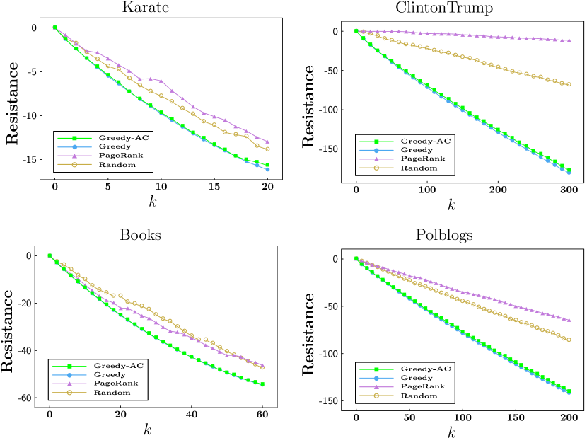
Figure 1. Resistance after performing four methods for node selection on datasets: Karate, Books, ClintonTrump and Polblogs for varying $k$. The initial opinions of nodes obey a uniform distribution.

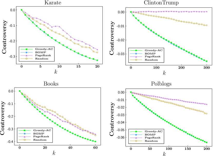
Figure 2. Controversy after performing four methods for node selection on datasets: Karate, Books, ClintonTrump and Polblogs for varying $k$. The initial opinions of nodes obey a uniform distribution.

We continue to demonstrate the effectiveness of our algorithm Greedy-AC for optimizing the controversy, by comparing it with three baseline schemes, PageRank, Random, and BOMP in (Matakos et al., 2017). Figure 2 illustrates the results for the four methods of node selection on the same four networks as in Figure 1. From Figure 2, one can observe that the decrease of the controversy yielded by Greedy-AC and BOMP are almost the same, and are very close to the optimal solutions according to the experimental results reported in (Matakos et al., 2017). Moreover, both Greedy-AC and BOMP are significantly better than PageRank and Random.

We note that Figures 1 and 2 only report the results for the case that the initial opinions of nodes follow a uniform distribution. For the cases that initial opinions obey an exponential distribution or a power-law distribution, the results are similar to those in Figures 1 and 2. We omit these results due to the space limit.

7.3. Comparison of Running Time

Although both Greedy-AC and BOMP achieve remarkable effectiveness for optimizing the controversy, we now show that Greedy-AC runs much faster than BOMP. To this end, we compare the running time of Greedy-AC with that of BOMP on $18$ real-world networks. For each network, we select $k=50$ nodes to minimize the controversy by using BOMP and Greedy-AC, respectively. In Table 1, we provide the results of running time and the drop of the controversy $\Delta C(\mathcal{G})$ for the two strategies. Table 1 shows that Greedy-AC is significantly faster than BOMP for those networks with more than 1400 nodes. The improvement of efficiency of Greedy-AC over BOMP becomes more significant when the graphs grow in size, and the speed-up of Greedy-AC is up to $20\times$. It is worth noting that BOMP is not applicable to the last nine networks marked with ”$*$” due to the limitations of time and memory. In comparison, Greedy-AC is scalable to large networks with more than $10^{6}$ nodes.

In spite the fact that in comparison with BOMP our Greedy-AC algorithm achieves significant improvement in the terms of efficiency, we will show the results returned by Greedy-AC are close to those for BOMP, besides the four aforementioned networks. To show this, we measure the relative error $\Gamma=|\tilde{\beta}-\beta|/\beta$ of the result for Greedy-AC on every network in Table 1, where $\beta$ and $\tilde{\beta}$ are the decrease of controversy $\Delta C(\mathcal{G})$ corresponding to Greedy-AC and BOMP, respectively. From the relative errors reported in Table 1, we observe that these relative errors are negligible for all tested networks, with the largest value equal to $2.74\%$. Thus, the results returned by Greedy-AC are very close to those associated with BOMP, implying that Greedy-AC is both effective and efficient, independent on the distributions of initial opinions.

We also present an extensive comparison of the performance of our two algorithms Greedy and Greedy-AC for optimizing the resistance, in terms of the efficiency and effectiveness. In Table 2, we report their running time and relative errors on various real-world networks. Table 2 indicates that Greedy-AC returns similar results as Greedy, but runs much faster than Greedy. Thus, Greedy-AC always achieves ideal performance irrespective of the distributions of initial opinions, in the contexts of both efficiency and effectiveness.

8. Conclusion

In this paper, we addressed the problem of minimizing risk of conflict, including controversy and resistance, by strategically changing the initial opinions of a small number of individuals. We unified the two optimization problems into one framework, and showed that the objective function is monotone and supermodular. We then presented two greedy algorithms to solve the optimization problem. The former returns a $(1-1/e)$ approximation to the optimum solutions in time $O(n^{3})$, while the latter provides a $(1-1/e-\epsilon)$ approximation in time $\widetilde{O}(mk\epsilon^{-2})$ for a positive parameter $\epsilon$. On the theoretic side, we provided detailed analysis of the approximation guarantee for the latter algorithm. On the experimental side, we performed extensive experiments on real-life networks, demonstrating that both of our algorithms lead to almost optimal solutions, and consistently outperform several alternative baseline heuristics. Particularly, our second algorithm yields a good approximation solution quickly on networks with more than two million nodes within $40$ minutes, demonstrating excellent scalablity to large-scale networks.

References

- (1)
- Abebe et al. (2018) Rediet Abebe, Jon Kleinberg, David Parkes, and Charalampos E Tsourakakis. 2018. Opinion dynamics with varying susceptibility to persuasion. In Proceedings of the 24th ACM SIGKDD International Conference on Knowledge Discovery and Data Mining. ACM, 1089–1098.
- Achlioptas (2001) Dimitris Achlioptas. 2001. Database-friendly random projections. In Proceedings of the 20th ACM SIGMOD-SIGACT-SIGART Symposium Principles of Database System. ACM, 274–281.
- Amelkin and Singh (2019) Victor Amelkin and Ambuj K Singh. 2019. Fighting opinion control in social networks via link recommendation. In Proceedings of the 25th ACM SIGKDD International Conference on Knowledge Discovery and Data Mining. ACM, 677–685.
- Anderson and Ye (2019) Brian DO Anderson and Mengbin Ye. 2019. Recent advances in the modelling and analysis of opinion dynamics on influence networks. International Journal of Automation and Computing 16, 2 (2019), 129–149.
- Bindel et al. (2015) David Bindel, Jon Kleinberg, and Sigal Oren. 2015. How bad is forming your own opinion? Games and Economic Behavior 92 (2015), 248–265.
- Brandes (2001) Ulrik Brandes. 2001. A faster algorithm for betweenness centrality. Journal of Mathematical Sociology 25, 2 (2001), 163–177.
- Chan et al. (2019) TH Chan, Zhibin Liang, and Mauro Sozio. 2019. Revisiting opinion dynamics with varying susceptibility to persuasion via non-convex local search. In Proceedings of the 28th World Wide Web Conference. ACM, 173–183.
- Chebotarev (2008) Pavel Chebotarev. 2008. Spanning forests and the golden ratio. Discrete Applied Mathematics 156, 5 (2008), 813–821.
- Chebotarev and Shamis (1997) P. Yu Chebotarev and E. V. Shamis. 1997. The matrix-forest theorem and measuring relations in small social groups. Automation and Remote Control 58, 9 (1997), 1505–1514.
- Chebotarev and Shamis (1998) P. Yu Chebotarev and E. V. Shamis. 1998. On proximity measures for graph vertices. Automation and Remote Control 59, 10 (1998), 1443–1459.
- Chen et al. (2018) Xi Chen, Jefrey Lijffijt, and Tijl De Bie. 2018. Quantifying and minimizing risk of conflict in social networks. In Proceedings of the 24th ACM SIGKDD International Conference on Knowledge Discovery and Data Mining. ACM, 1197–1205.
- Das et al. (2013) Abhimanyu Das, Sreenivas Gollapudi, Rina Panigrahy, and Mahyar Salek. 2013. Debiasing social wisdom. In Proceedings of the 19th ACM SIGKDD international conference on Knowledge discovery and data mining. ACM, 500–508.
- DeGroot (1974) Morris H DeGroot. 1974. Reaching a consensus. Journal of Mathematical Sociology 69, 345 (1974), 118–121.
- Dong et al. (2018) Yucheng Dong, Min Zhan, Gang Kou, Zhaogang Ding, and Haiming Liang. 2018. A survey on the fusion process in opinion dynamics. Information Fusion 43 (2018), 57–65.
- Friedkin and Johnsen (1990) Noah E Friedkin and Eugene C Johnsen. 1990. Social influence and opinions. Journal of Mathematical Sociology 15, 3-4 (1990), 193–206.
- Gaitonde et al. (2020) J. Gaitonde, J. Kleinberg, and Éva Tardos. 2020. Adversarial perturbations of opinion dynamics in networks. In Proceedings of the 21st ACM Conference on Economics and Computation. ACM, 471–472.
- Garimella et al. (2017) Kiran Garimella, Gianmarco De Francisci Morales, Aristides Gionis, and Michael Mathioudakis. 2017. Reducing controversy by connecting opposing views. In Proceedings of the 10th ACM International Conference on Web Search and Data Mining. ACM, 81–90.
- Gionis et al. (2013) Aristides Gionis, Evimaria Terzi, and Panayiotis Tsaparas. 2013. Opinion maximization in social networks. In Proceedings of the 2013 SIAM International Conference on Data Mining. SIAM, 387–395.
- Golender et al. (1981) VE Golender, VV Drboglav, and AB Rosenblit. 1981. Graph potentials method and its application for chemical information processing. Journal of Chemical Information and Computer Sciences 21, 4 (1981), 196–204.
- Haddadan et al. (2021) Shahrzad Haddadan, Cristina Menghini, Matteo Riondato, and Eli Upfal. 2021. RePBubLik: Reducing polarized bubble radius with link insertions. In Proceedings of the 14th ACM International Conference on Web Search and Data Mining. ACM, 139–147.
- Jia et al. (2015) Peng Jia, Anahita MirTabatabaei, Noah E Friedkin, and Francesco Bullo. 2015. Opinion dynamics and the evolution of social power in influence networks. SIAM Rev. 57, 3 (2015), 367–397.
- Johnson and Lindenstrauss (1984) William B Johnson and Joram Lindenstrauss. 1984. Extensions of Lipschitz mappings into a Hilbert space. Communications In Contemporary Mathematics 26, 189-206 (1984), 1.
- Kunegis (2013) Jérôme Kunegis. 2013. Konect: the koblenz network collection. In Proceedings of the 22nd World Wide Web Conference. ACM, 1343–1350.
- Kyng and Sachdeva (2016) Rasmus Kyng and Sushant Sachdeva. 2016. Approximate Gaussian elimination for Laplacians-fast, sparse, and simple. In Proceedings of the 57th IEEE Symposium on Foundations of Computer Science. IEEE, 573–582.
- Leskovec and Sosič (2016) Jure Leskovec and Rok Sosič. 2016. SNAP: A general-purpose network analysis and graph-mining library. ACM Transactions on Intelligent Systems and Technology 8, 1 (2016), 1.
- Li and Schild (2018) Huan Li and Aaron Schild. 2018. Spectral subspace sparsification. In Proceedings of the 59th IEEE Annual Symposium on Foundations of Computer Science. IEEE, 385–396.
- Mackin and Patterson (2019) Erika Mackin and Stacy Patterson. 2019. Maximizing diversity of opinion in social networks. In Proceedings of the 2019 American Control Conference. IEEE, 2728–2734.
- Matakos et al. (2017) Antonis Matakos, Evimaria Terzi, and Panayiotis Tsaparas. 2017. Measuring and moderating opinion polarization in social networks. Data Mining and Knowledge Discovery 31, 5 (2017), 1480–1505.
- Matakos et al. (2020) Antonis Matakos, Sijing Tu, and Aristides Gionis. 2020. Tell me something my friends do not know: Diversity maximization in social networks. Knowledge and Information Systems 62, 9 (2020), 3697–3726.
- Merris (1997) Russell Merris. 1997. Doubly stochastic graph matrices. Publikacije Elektrotehničkog Fakulteta. Serija Matematika 1, 8 (1997), 64–71.
- Musco et al. (2018) Cameron Musco, Christopher Musco, and Charalampos E Tsourakakis. 2018. Minimizing polarization and disagreement in social networks. In Proceedings of the 27th World Wide Web Conference. ACM, 369–378.
- Nemhauser et al. (1978) George L. Nemhauser, Laurence A. Wolsey, and Marshall L. Fisher. 1978. An analysis of approximations for maximizing submodular set functions - I. Mathematical Programming 14, 1 (1978), 265–294.
- Ravazzi et al. (2015) Chiara Ravazzi, Paolo Frasca, Roberto Tempo, and Hideaki Ishii. 2015. Ergodic Randomized Algorithms and Dynamics Over Networks. IEEE Transactions on Control of Network Systems 1, 2 (2015), 78–87.
- Semonsen et al. (2019) Justin Semonsen, Christopher Griffin, Anna Squicciarini, and Sarah Rajtmajer. 2019. Opinion dynamics in the presence of increasing agreement pressure. IEEE Transactions on Cybernetics 49, 4 (2019), 1270–1278.
- Spielman and Teng (2014) D. Spielman and S. Teng. 2014. Nearly linear time algorithms for preconditioning and solving symmetric, diagonally dominant linear systems. SIAM J. Matrix Anal. Appl. 35, 3 (2014), 835–885.
- Spielman and Srivastava (2011) Daniel A Spielman and Nikhil Srivastava. 2011. Graph sparsification by effective resistances. SIAM J. Comput. 40, 6 (2011), 1913–1926.
- Tu et al. (2020) Sijing Tu, Cigdem Aslay, and Aristides Gionis. 2020. Co-exposure maximization in online social networks. In Proceedings of the 33rd Advances in Neural Information Processing Systems. 3232–3243.
- Xu et al. (2020) Pinghua Xu, Wenbin Hu, Jia Wu, and Weiwei Liu. 2020. Opinion maximization in social trust networks. In Proceedings of the 29th International Joint Conference on Artificial Intelligence. 1251–1257.
- Xu et al. (2021) Wanyue Xu, Qi Bao, and Zhongzhi Zhang. 2021. Fast evaluation for relevant quantities of opinion dynamics. In Proceedings of the Web Conference. ACM, 2037–2045.
- Yi and Patterson (2020) Yuhao Yi and Stacy Patterson. 2020. Disagreement and polarization in two-party social networks. IFAC-PapersOnLine 53, 2 (2020), 2568–2575.
- Zhang and Liu (2017) Lei Zhang and Bing Liu. 2017. Sentiment Analysis and Opinion Mining. Encyclopedia of Machine Learning and Data Mining (2017), 1152–1161.