Average Communication Rate for Event-Triggered Stochastic Control Systems

Abstract

Quantification of the triggering rates of an event-triggered stochastic system with deterministic thresholds is a challenging problem due to the non-stationary nature of the system’s stochastic processes. A typical example is the computation of the average communication rate (ACR) of the networked event-triggered stochastic control systems (ET-SCS) of which the communication of the sensor network is scheduled by whether a system variable of interest exceeds predefined constant thresholds. For such a system, a closed-loop effect emerges due to the interdependence between the system variable and the trigger of communication. This effect, commonly referred to as side information by related work, distorts the stochastic distribution of the system variables and makes the ACR computation non-trivial. Previous work in this area used to over-simplify the computation by ignoring the side information and misusing a Gaussian distribution, which leads to approximated results. This paper proposes both analytical and numerical approaches to predict the exact ACR for an ET-SCS using a recursive model. Furthermore, we use theoretical analysis and a numerical study to qualitatively evaluate the deviation gap of the conventional approach that ignores the side information. The accuracy of our proposed method, alongside its comparison with the simplified results of the conventional approach, is validated by experimental studies. Our work is promising to benefit the efficient resource planning of networked control systems with limited communication resources by providing accurate ACR computation.

I Introduction

In recent years, emerging networked control systems, such as intelligent industrial manufacturing [1], smart power grids [2], and autonomous vehicles [3], are characterized by a distributed design manner where the plants and the sensors are located remotely and are connected with a common network. The development of the closed-loop controllers for these systems requires sufficient sampling of the system states ensured by active communication of the network, such that the controllers always have access to the latest system states provided by the remote sensors through the network. Nevertheless, the communication resources of the networked systems are often limited by the power restrictions of the system, especially for the mobile and portable devices of which the power mainly rely on batteries. This issue suggests reducing the frequency of state sampling by properly scheduling the communication of the network. This was conventionally solved with time-based schemes which later gave way to event-based schemes.

It is argued in [4] that the event-based scheduling schemes can achieve the same performance as the periodic time-based ones but with considerably less consumption of communication resources. This finding motivates the development of different event-based scheduling schemes, including the stochastic, periodic, and deterministic event-based ones, for various networked systems [5, 6, 7]). The event-based schemes have shown superior efficiency, high flexibility, and quick responsiveness incorporating the restriction of communication resource limitations [8, 9, 10, 11]. A typical event-based scheduling scheme is illustrated in Fig. 1, where the sampling of the system state or the activation of the communication is governed by a scheduler that triggers a time-asynchronous event. This event does not explicitly depend on time but is associated with a system variable of interest and a predefined threshold. Thus, the scheduling is performed in a time-asynchronous manner which activates the communication only when necessary. The necessity of communication is determined by a certain triggering event, which intermittently closes the loop between the controlled system and the sensor. This ensures efficient consumption of the communication resources [12, 13, 14, 15, 16].

Figure 1: A typical event-based communication scheduler for a networked system. The dashed line indicates remote sensing, such as infra-sensing or visual perception. The switch symbol denotes the communication status $\delta_{t}$ (active or inactive) of the network. $\mathcal{S}_{t}$ is the sampled system state, $\mathcal{V}_{t}$ is the system variable of interest, and $\mathscr{E}\!\left(\mathcal{V}_{t},\eta\right)$ represents the event that triggers the communication based on a given threshold $\eta$.

One of the main purposes of investigating communication scheduling schemes for networked systems is for the efficient planning of communication resources. Compared to the time-based scheduling schemes, the resource planning for the event-based ones is usually less straightforward and more challenging due to asynchronous state sampling. A typical index that facilitates communication resource planning is communication rate (CR) which depicts the likelihood of active communication at a certain time [17], i.e., the probability of the communication switch in Fig. 1 being closed. CR provides a practical insight into how many system resources are allocated to network communication and supports the efficient planning of system resources. In most applications, the communication status is a random variable incorporating stochastic system uncertainties. Thus, what attracts us is typically the average communication rate (ACR) which refers to the expected value of active communication. Particular attention has been attracted to the stationary ACR [18] which represents the limit of the ACR as the time approaches infinity. It is often used to evaluate the consumption of communication resources in the steady state of a networked system. Conventionally, the computation of the ACR is solved using statistical methods via numerical experiments, such as a Monte Carlo experiment. The analytical solution of the ACR with a closed form is a challenging problem due to the closed-loop effect of the event-based scheduling scheme, also known as side information [19].

In Fig. 1, the closed-loop effect, or side information, refers to the interdependence between the triggering event and the system variable of interest, which forms a closed loop between the system and the scheduler (the blue path). This closed-loop distorts the distributions of the system variables, such that they are no more subject to trivial Gaussian distributions even though the system uncertainties are formulated as Gaussian. Analyzing the stochastic property of the communication status is thus challenging since it is difficult to track the probabilistic propagation of the system variables. In the literature, analytical computation methods for the ACR are quite sparse. They only show up in a few papers that mainly focus on the control and filtering of networked systems [20, 21, 22, 17, 6, 23]. These approaches either over-simplify the computation of the ACR by imposing impractical assumptions or conduct conservative and coarse approximations. Their results can hardly be used to predict exact ACR which is important to efficient resource planning for networked communication systems. In [20, 17], the ACR is computed by ignoring the closed-loop effect and approximating the distribution of the concerned system variable with a Gaussian distribution, which, however, leads to an accuracy gap with the true ACR. The work in [22] provides lower and upper bounds for the ACR without giving its analytical form. In [6, 23], the computation of ACR is simplified by involving a stochastic triggering threshold which has obvious shortcomings compared to deterministic thresholds due to the inferior control performance and the sensitivity to data loss. To our best knowledge, the accurate computation of ACR for an event-triggered networked system with deterministic triggering thresholds has not been addressed in the literature, although it is a fundamental step towards the study of the crucial filtering problem [22, 24, 25, 26, 27].

As mentioned, the fundamental challenge of accurately quantifying the ACR for an event-triggered networked system is the precise tracking of the probabilistic propagation of the system variables of interest under the closed-loop effect. From a mathematical perspective, the event-based scheduling scheme with deterministic thresholds imposes constant truncation to the support set of the probabilistic distribution functions (PDF) of the concerned system variables at each sampling instant. This truncation operation constantly removes the Gaussianity of the system variables. Thus, the critical technical point of accurately computing the ACR is to precisely depict the truncated PDFs of the system variables recursively over time, which formulates a challenging mathematical problem. The main goal of this work is to overcome this challenge and provide accurate computation methods for the ACR of a typical networked system, an event-triggered stochastic control system (ET-SCS), where the communication is triggered when the state estimation error exceeds a deterministic threshold. To support this, we propose a recursive model that exactly depicts the temporal evolution of ACR based on the model raised in [17]. Using this recursive model, we are able to track the truncated PDF of the system variables at each sampling time and investigate its influence on the ACR. Based on this, we are able to compute the ACR at an arbitrary instant using a finite number of coefficients. We also prove the existence of the stationary ACR and calculate its value using these coefficients. Considering the complexity of the proposed analytical method, we further raise a numerical counterpart algorithm to calculate the ACR recursively. Both theoretical analysis and experimental studies are conducted to verify the accuracy of the proposed methods and qualify the inaccuracy gap of the conventional methods [20, 21, 22, 17, 6, 23]. The main contributions of this article are summarized below.

1. Proposing a novel recursive temporal-evolution model for the ACR of a generic ET-SCS.

2. Proving the existence of the stationary ACR for a generic ET-SCS with deterministic event-triggered thresholds.

3. Providing an analytical method and a numerical algorithm for the computation of ACR for a generic ET-SCS.

4. Conducting theoretical and numerical studies to qualify the accuracy gap of the conventional method.

5. Validating the feasibility and accuracy of the proposed methods using a case study.

The rest of this article is organized as follows. Sec. II formulates the problem, with mathematical preliminaries provided. In Sec. III, we introduce the recursive model of the ACR and investigate the existence of the stationary ACR. Sec. IV presents the methods to precisely compute the ACR. In Sec. V, we use theoretical analysis and a numerical example to verify the accuracy of the proposed method and evaluate the accuracy gap of the conventional method. In Sec. VI, a numerical experiment on a simple vehicle-following case is conducted to validate our methods. Finally, Sec. VII concludes the article.

Notation: The rest of this article obeys the following notations. The sets of real and natural numbers are denoted by $\mathbb{R}$ and $\mathbb{N}$. The superscript ⁺ sued after them indicates the subsets only containing the positive elements. A Gaussian distribution with mean value $\mu\in\mathbb{R}$ and variance $\sigma^{2}$, $\sigma\in\mathbb{R}^{+}$ is represented by $\mathcal{N}(\mu,\sigma^{2})$. For a stochastic event $\mathscr{E}$ defined on a probability space, $P(\mathscr{E})$ denotes the occurring probability of $\mathscr{E}$. For a stochastic variable $z\!\in\mathbb{R}$, $P(z)$, $p_{z}(\cdot)$, $F_{z}(\cdot)$, $\mathsf{E}(z)$, and $\mathrm{Var}(z)$ denote, respectively, its probability, PDF, cumulative distribution function (CDF), expectation, and variance.

II Problem Statement and Preliminaries

In this section, we describe the main mathematical problem of this paper and provide the preliminaries for its solution. First, we introduce the dynamical model of an ET-SCS and the definition of the ACR, followed by the problem statement. Then, we revisit the Jury’s stability criterion and the stochastic properties of truncated random variables which are important to the analysis of the ACR in the next sections.

II-A Dynamic Model of ET-SCS and State Estimation Error

As shown in Fig. 2, the ET-SCS considered in this article is composed of a plant and a series of sensors which are connected with a common network. In this paper, we investigate a scalar ET-SCS, where the dynamic model of the plant is assumed to be linear time-invariant (LTI) and depicted by the following scalar stochastic difference equation (SDE),

$$x_{k+1}=Ax_{k}+Bu_{k}+w_{k},$$ (1)

where $k\in\mathbb{N}$ denotes the discrete sampling time of the system, $x_{k},u_{k}\in\mathbb{R}$ are, respectively, the state and control input of the system at time $k$, $A,B\in\mathbb{R}$ are constant parameters, and $w_{k}\!\in\mathbb{R}$ is the stochastic noise of the system. For simplicity, we assume that the initial state of the system $x_{0}$ is a known deterministic variable. Note that the stochastic process $w_{k}$, $k\in\mathbb{N}$, is subject to the following assumption.

Assumption 1.

The Gaussian stochastic process $w_{k}$ is independent and identically distributed (i.i.d.) for all $k\in\mathbb{N}$, i.e.,

1. $w_{k}\sim\mathcal{N}\!\left(0,\sigma^{2}\right)$, $\forall\,k\in\mathbb{N}$, with $\sigma\in\mathbb{R}^{+}$.

2. $p_{w,w}(w_{i},w_{j})\!=\!p_{w}(w_{i})p_{w}(w_{j})$ holds for all $i,j\!\in\!\mathbb{N}$, $i\!\neq\!j$, where $p_{w}(\cdot)$ is the PDF of stochastic variable $w_{k}$, $k\in\mathbb{N}$, and $p_{w,w}(\cdot,\cdot)$ is the joint PDF of $w_{i}$ and $w_{j}$, $i,j\in\mathbb{N}$.

Figure 2: The block diagram of an ET-SCS.

Remark 1.

Our work in this paper only deals with a scalar ET-SCS. Note that the exact computation of the ACR for a multi-dimensional ET-SCS is even more challenging due to the probabilistic coupling among the individual dimensions of the non-Gaussian system variables. Also, various triggering options for multi-dimensional system variables make it tedious to determine their analytical distribution functions. The study on a scalar ET-SCS is sufficient to draw essential quantitative and qualitative conclusions that can be extended to multi-dimensional systems with additional efforts in future work.

For system (1), its state $x_{k}$ at any time $k\in\mathbb{N}^{+}$ can be measured by one or multiple sensors. However, the state is sampled for the system plant only when the network communication is active, indicated by a closed switch in Fig. 2. At the time $k$, whether the status of the communication is active or not is represented as a binary event $\delta_{k}\in\{0,1\}$, namely $\delta_{k}=1$ for active and $\delta_{k}=0$ for inactive. For brevity, we represent these conditions as $\delta_{k}^{\{1\}}$ and $\delta_{k}^{\{0\}}$. The communication status $\delta_{k}$ is affected by an event $\mathscr{E}_{k}$ which is produced by an event-based scheduler which will be introduced in Sec II-B. When the system state is not sampled, an estimated value $\hat{x}_{k}$ is provided by a state estimator utilizing the system model (1) and the history data $\mathcal{I}_{k-1:\iota}=\left\{\delta_{k-1},\cdots,\delta_{\iota+1},\delta_{\iota},x_{\iota},u_{k-1},\cdots,u_{\iota}\right\}$ [7],

$$\begin{split}\hat{x}_{\iota}=&\,x_{\iota}\\ \hat{x}_{\iota+1}=&\,Ax_{\iota}+Bu_{\iota},\\ \cdots&\,\\ \hat{x}_{i}=&\,A\hat{x}_{i-1}+Bu_{i-1},\end{split}$$ (2)

$i=\iota+2,\cdots,k$, where $\iota\in\mathbb{N}$ refers to the last instant of state sampling and equation $\hat{x}_{\iota}=x_{\iota}$ indicates a state sampling operation. Since the initial state $x_{0}$ is deterministic and known, we have $\hat{x}_{0}=x_{0}$ and $e_{0}=0$. The history data $\mathcal{I}_{k-1:\iota}$ is stored in a memory on the plant. All the system data before the last instant, i.e., all $\{\delta_{i},x_{i},u_{i}\}$ where $i<\iota$, is timely abandoned. Thus, a feedback controller $u_{k}=u(\hat{x}_{k}-r_{k})$ can be designed to achieve the desired closed-loop performance. The performance of the feedback controller is not within the scope of this paper. We make a correspondence between the ET-SCS in Fig. 2 and the general event-based networked system in Fig. 1 by recognizing $x_{k}$ as the system state and the estimation error $e_{k}=x_{k}-\hat{x}_{k}$ as the system variable of interest.

By subtracting (2) from (1), we obtain the dynamic model of the state estimation error as

$$\begin{split}e_{\iota}=&\leavevmode\nobreak\ 0,\\ e_{\iota+1}=&\leavevmode\nobreak\ w_{\iota},\\ \cdots&\\ e_{i}=&\leavevmode\nobreak\ Ae_{i-1}+w_{i-1},\end{split}$$ (3)

where $i=\iota+2,\cdots,k$. Therefore, for all $i=\iota+1,\cdots,k$, $e_{i}$ is a random variable. Substituting $e_{k-1}$, $e_{k-2}$, $\cdots$, $e_{\iota}$ to $e_{k}$ recursively, we obtain

$$\textstyle e_{k}=\sum_{i=\iota}^{k-1}A^{k-i-1}w_{i},\leavevmode\nobreak\ k>\iota.$$ (4)

The dynamic model (3) indicates that the estimation error accumulates over the time interval $\{\iota+1,\iota+2,\cdots,k\}$ due to the lack of state sampling. The error accumulation may lead to the degradation of the system control performance. Meanwhile, equation (4) shows that $e_{k}$ is subject to a Gaussian distribution $\mathcal{N}\!\left(0,\sum_{i=\iota}^{k-1}\!A^{2(k-i-1)}\right)$ considering the property of the linear combination of Gaussian stochastic variables. Nevertheless, we should note that (3) and (4) only hold when the state estimation error and the triggering event are subject to an open-loop configuration. In Fig. 2, this pertains to the scenario where the Scheduler is designed such that its output $\mathscr{E}_{k}$ is independent of its input $e_{k}$. Next, we will show that (3) and (4) do not generally hold and $e_{k}$ is no more a Gaussian-distributed stochastic variable for an event-triggered scheduler.

II-B Event-Triggered Scheduling and Closed-Loop Effect

To restrict the accumulation of the state estimation error $e_{k}$, $k\in\mathbb{N}^{+}$, by fully exploiting the communication resources, the scheduler performs a least-necessary principle meaning that the communication is only activated when either the last state estimation error $e_{k-1}$ exceeds a predefined threshold $\eta\in\mathbb{R}^{+}$, or the consecutive inactive period is beyond a time limit $T\in\mathbb{N}^{+}$, i.e., for all $k\in\mathbb{N}^{+}$ and $\iota\in\mathbb{N}$, $\iota<k$,

$$\delta_{k}=\begin{cases}1,&\qquad\text{if}\quad|e_{k-1}|\geq\eta\leavevmode\nobreak\ \text{or}\leavevmode\nobreak\ k-\iota>T\\ 0,&\qquad\text{otherwise},\end{cases}$$ (5)

where the condition that triggers active communication $\delta_{k}^{\{1\}}$ refers to a positive event $\mathscr{E}_{k}$, otherwise a negative event $\overline{\mathscr{E}}_{k}$. The scheduling scheme (5) maintains a decent system performance by ensuring low resource usage by limiting the frequency of communication while restricting the estimation errors. Such an event-based scheduling model is widely used in various networked control systems, such as platooning of a group of vehicles [28, 29], power systems [30, 31] and cooperative manipulation in robotics systems [32, 33].

The result of the event-triggering scheduling scheme (5) is a closed loop between the triggering event $\mathscr{E}_{k}$, or the communication status $\delta_{k}$ and the state estimation error $e_{k}$ (the blue path in Fig. 2). This loop has a significant influence on the probabilistic distribution of the estimation error $e_{k}$. Specifically, the error accumulation depicted in (3) only occurs when $|e_{i}|\leq\eta$, for any $i=\iota,\iota+1,\cdots,k-1$. Otherwise, any $|e_{i}|>\eta$ will immediately activate the state sampling and lead to $\delta_{i+1}=1$ and $e_{i+1}=0$. Thus, given the last communication instant $\iota$ and the history data $\mathcal{I}_{k-1:\iota}$, the estimation error under the event-triggered scheduling scheme (5) becomes

$$\begin{split}\hat{e}_{\iota}=&\leavevmode\nobreak\ 0,\\ \hat{e}_{\iota+1}=&\leavevmode\nobreak\ w_{\iota},\\ \cdots&\\ \hat{e}_{i}=&\left\{\begin{array}[]{ll}A\hat{e}_{i-1}+w_{i-1},\nobreak\leavevmode&\mathrm{if}\,|\hat{e}_{i-1}|<\eta,\\ 0,\nobreak\leavevmode&\mathrm{else},\end{array}\right.\end{split}$$ (6)

where $i=\iota+2,\cdots,k$, for all $k\leq\iota+T$. Here, we use a new symbol $\hat{e}_{i}$ to represent this closed-loop state estimation error, or closed-loop error under the event-triggered scheduling scheme (5) to distinguish it from the open-loop error $e_{i}$ in (3). Similar to $e_{i}$, $\hat{e}_{i}$ is also a random variable, for $i=\iota+1,\iota+2,\cdots,k$. Differently, the closed-loop error (6) contains additional side information $|\hat{e}_{i-1}|<\eta$ compared to the open-loop error (3). This side information imposes a truncation operation on the probabilistic distribution of the closed-loop error at every sampling instant. It breaks the linearity of the dynamic model of the state estimation error and distorts its stochastic propagation. As a result, the closed-loop error is hardly subject to a Gaussian distribution as time increases, even though the noise is a stationary Gaussian process according to Assumption 1. Also, it is difficult to bring up a brief overall analytical form to represent $\hat{e}_{k}$, similar to (4), which makes it difficult to track the distorted stochastic propagation. In this paper, we refer to the fact that the side information distorts the stochastic propagation of the system variable of interest as the closed-loop effect. In Sec. II-E, we will briefly introduce the effect of a truncation operation on a random variable.

II-C Stationary and Transient ACR of an ET-SCS

For the ET-SCS in (1) with the state estimator (2) and the event-triggered scheduler (5), the ACR is defined as

$$\mathsf{E}\!\left(\delta_{k}\right)=P(\delta_{k}^{\{1\}}),\leavevmode\nobreak\ k\in\mathbb{N}$$ (7)

which depicts the likelihood of the active status of the communication, or, equivalently, the realization of the event $\delta_{k}^{\{1\}}$. Meanwhile, the ACR denotes the probability of the state sampling. Since the initial state $x_{0}$ is deterministic and known, we have $\mathsf{E}(\delta_{0})=P(\delta_{0}^{\{1\}})=1$. Also, given $\hat{e}_{0}=x_{0}-\hat{x}_{0}=0$, we know $\mathsf{E}(\delta_{1})=P(\delta_{1}^{\{1\}})=0$. For any $k\in\mathbb{N}^{+}$, $k\geq 2$, however, the value of $\delta_{k}$ is usually random, and the ACR is computed as

$$\textstyle\mathsf{E}\!\left(\delta_{k}\right)=1-P(\delta_{k}^{\{0\}})=1-\int_{-\eta}^{\eta}p_{\hat{e}_{k-1}}(z)\mathrm{d}z,$$ (8)

where $p_{\hat{e}_{k}}(\cdot)$ is the PDF of the state estimation error and $z\in\mathbb{R}$ is an auxiliary variable. Note that the integration interval $[\,-\eta,\eta\,]$ corresponds to the constraint $|\hat{e}_{k-1}|<\eta$ in (5) which blocks state sampling at time $k$.

Remark 2.

The above statements are based on our assumption that the initial system state $x_{0}$ is known. Otherwise, the values of $E(\delta_{0})$ and $E(\delta_{1})$ are neither $1$ nor $0$. Instead, they are dependent on the distribution of $x_{0}$ and should be valued within the interval $(0,\,1)$.

The limit $\mathsf{E}(\delta_{\infty})=\displaystyle\lim_{k\rightarrow\infty}\mathsf{E}(\delta_{k})$, if it exists, is defined as the stationary ACR, while $\mathsf{E}(\delta_{k})$ for a finite $k\in\mathbb{N}$ is referred to as the transient ACR. The main issue of exactly calculating the stationary and the transient ACR is that the analytical form of the PDF $p_{\hat{e}_{k}}(\cdot)$, $k\in\mathbb{N}$, is difficult to derive due to the challenge of capturing the nontrivial stochastic propagation of the closed-loop errors, as introduced in Sec. II-B. In some existing work [17, 23], $p_{\hat{e}_{k}}(\cdot)$ is approximated by a Gaussian distribution by ignoring the closed-loop effect, which leads to the approximated calculation of ACR. We show in this article that such approximation results in a larger value of ACR compared to the truth. Alongside this, accurate ACR computation methods are also provided.

II-D Existence of Steady State of A Discrete-Time LTI System

To verify the existence of the stationary ACR for an ET-SCS, in this paper, we construct a recursive model to depict the timed evolution of the ACR. The recursive ACR model is indeed a discrete-time LTI (dt-LTI) system and the stationary ACR is equivalent to its steady state. This allows us to solve the stationary ACR by investigating the asymptotic stability of a general dt-LTI system, which can be examined by the well-known Jury stability criterion [34]. Consider a characteristic polynomial with variable $z\in\mathbb{R}$ in the following form,

$$D(z)=a_{0}+a_{1}z+a_{2}z^{2}+\ldots+a_{N}z^{N},$$

where $N\in\mathbb{N}^{+}$ is the degree of the characteristic polynomial and $a_{i}\in\mathbb{R}$, $i=1,2,\cdots,N$, are coefficients. The following tests determine whether the system represented by $D(z)$ has any pole outside the unit circle (the instability region). A system must conform to all the following rules to be considered stable.

Rule 1: If $z=1$, $D(z)>0$ must hold.

Rule 2: If $z=-1$, $z^{N}D(z)>0$ must hold.

Rule 3: $|a_{0}|<|a_{N}|$ must hold.

If all rules satisfied, we expand the Jury Array as follows.

1)	$a_{0}$	$a_{1}$	$a_{2}$	$a_{3}$	…	$a_{N}$
2)	$a_{N}$	…	$a_{3}$	$a_{2}$	$a_{1}$	$a_{0}$
3)	$b_{0}$	$b_{1}$	$b_{2}$	…	$b_{N-1}$
4)	$b_{N-1}$	…	$b_{2}$	…	$b_{0}$
⋮	⋮	⋮	⋮
$2N-3$)	$v_{0}$	$v_{1}$	$v_{2}$

Once we reach to a row with 2 members, we stop constructing further arrays. To calculate the values of the odd-number rows, we can use the following formula. The even number rows are equal to the previous row in reverse order. We will use $k$ as an arbitrary subscript value. These formulas are reusable for all elements in the array:

$$b_{k}=\begin{vmatrix}a_{0}&\!\!a_{N-k}\\ a_{N}&\!\!a_{k}\\ \end{vmatrix},c_{k}=\begin{vmatrix}b_{0}&\!\!b_{N-1-k}\\ b_{N-1}&\!\!b_{k}\\ \end{vmatrix},d_{k}=\begin{vmatrix}c_{0}&\!\!c_{N-2-k}\\ c_{N-2}&\!\!c_{k}\\ \end{vmatrix}.$$

This pattern can be carried out to all lower rows of the array, if necessary.

Rule 4: Once the Jury array has been formed, all the following relationships must be satisfied until the last row of the array

$$|b_{0}|>|b_{N-1}|,\leavevmode\nobreak\ \leavevmode\nobreak\ |c_{0}|>|c_{N-2}|,\leavevmode\nobreak\ \leavevmode\nobreak\ |d_{0}|>|d_{N-3}|.$$

The system is stable if all these conditions are satisfied.

II-E Truncated Stochastic Variables

As mentioned in Sec. II-C, the side information $|e_{k-1}|<\eta$ in (6) changes the support of $p_{\hat{e}_{k}}(\cdot)$ at every sampling instant $k$. With a constant threshold $\eta\in\mathbb{R}^{+}$, the change is specifically a symmetric truncation operation to the PDF $p_{\hat{e}_{k}}(\cdot)$. Consider a scalar stochastic variable $\zeta\in\mathbb{R}$ with an infinite-support PDF $p_{\zeta}(\cdot)$. We use $\zeta^{[a,b]}$ to represent the truncated stochastic variable derived from $\zeta$ by trimming its support set with a fixed interval $\zeta\in[\,a,b\,]$, $a,b\in\mathbb{R}$. Due to this truncation operation, the derived variable $\zeta^{[a,b]}$ has different stochastic properties compared to its original $\zeta$. Specifically, its PDF reads

$$p_{\zeta^{[a,b]}}\!\left(z\right)=\left\{\begin{array}[]{ll}\rho_{\zeta}(a,b)p_{\zeta}(z),&a\leq z\leq b,\\ 0,&\mathrm{otherwise},\end{array}\right.$$ (9)

where $z\in\mathbb{R}$ is an auxiliary variable, $p_{\zeta^{[a,b]}}(\cdot)$ denotes the PDF of $\zeta^{[a,b]}$ subject to a truncation interval $[\,a,b\,]$, and $\rho_{\zeta}(a,b)$ is a scalar calculated as

$$\rho_{\zeta}(a,b)=1/(F_{\zeta}(b)-F_{\zeta}(a))$$

where $F_{\zeta}(\cdot)$ is the cumulative distribution function (CDF) of $\zeta$. Also, the expected value and the variance of $\zeta^{[a,b]}$ are

$$\textstyle\mathsf{E}\!\left(\zeta^{[a,b]}\right)=\int^{b}_{a}zp_{\zeta^{[a,b]}}(z)\mathrm{d}z=\rho_{\zeta}(a,b)\int^{b}_{a}zp_{\zeta}(z)\mathrm{d}z,$$ (10)

$$\begin{split}\textstyle\mathrm{Var}\!\left(\zeta^{[a,b]}\right)=&\,\textstyle\int^{b}_{a}z^{2}p_{\zeta^{[a,b]}}(z)\mathrm{d}z-\mathsf{E}^{2}\!\left(\zeta^{[a,b]}\right)\\ =&\,\textstyle\rho_{\zeta}(a,b)\int^{b}_{a}z^{2}p_{\zeta}(z)\mathrm{d}z-\mathsf{E}^{2}\!\left(\zeta^{[a,b]}\right).\end{split}$$ (11)

Note that the difference between the mean values and the variances of a stochastic variable $\zeta$ and its truncated counterpart $\zeta^{[a,b]}$ is reflected not only by the additional multiplier $\rho_{\zeta}(a,b)$ but also by the changed upper and lower limits of the integrals, $a$ and $b$. If $\zeta$ is a Gaussian variable, $\zeta^{[a,b]}$ is not necessarily Gaussian. This means that all the properties that are proposed for Gaussian variables, such as the linear combination properties, may not hold for their truncated variables. Ignoring this effect may lead to the inaccurate characterization of the truncated stochastic variable.

III Communication rate analysis

In this section, we conduct a comprehensive analysis of the transient and the stationary ACR for an ET-SCS defined in (7). Based on the introduction of the predictive indexes and the predictive coefficients, we derive a recursive model for the transient ACR of an ET-SCS. Then, by showing the equivalence between the recursive model and a dt-LTI system, we prove the existence of the stationary ACR using the Jury stability criterion recalled in Sec. II-D. As a result, the transient and the stationary ACR can be calculated using a finite number of predictive coefficients.

III-A The Predictive Indexes and The Predictive Coefficients

In this section, we introduce the predictive indexes and the predictive coefficients which are important to analyze the ACR. We first define a compound event for $k,n\in\mathbb{N}^{+}$, $n\leq k$,

$$\mathscr{E}_{k:k-n}=\delta_{k}^{\{0\}}\cap\delta_{k-1}^{\{0\}}\cap\cdots\cap\delta_{k-n+1}^{\{0\}}\cap\delta_{k-n}^{\{1\}},$$ (12)

which represents the conjunction of $n$ successive inactive events after an active event $\delta_{k-n}^{\{1\}}$. It is straightforward to show that the compound event satisfies the following property.

Property 1.

For any $n,k\in\mathbb{N}^{+}$, $n\leq k$, event $\mathscr{E}_{k:k-n}$ satisfies the following conditions.

1. $\mathscr{E}_{k:k-n}\neq\varnothing$, $\forall\,n\leq T$, and $\mathscr{E}_{k:k-n}=\varnothing$, $\forall\,n>T$.

2. $\mathscr{E}_{k:k-i}\cap\mathscr{E}_{k:k-j}=\varnothing$, for any $i,j\leq k$, $i\neq j$.

3. $\bigcup_{n=1}^{k}\mathscr{E}_{k:k-n}=\delta_{k}^{\{0\}}$.

In Property 1, condition 1) is met considering that the non-communication period of the system should not be larger than the limit $T$, according to the event-triggered scheduler (5). Condition 2) is verified by the mutual exclusion between the compound events. Condition 3) is justified by taking the union of all compound events $\mathscr{E}_{k:k-n}$, for all $n=1,2,\cdots,k$.

III-A1 Predictive indexes

For particular communication variables $\delta_{0}$, $\delta_{1}$, $\cdots$, $\delta_{n}$, we define $n$-step predictive non-communication index $P_{n}$, or predictive index as

$$P_{n}=P\!\left(\left.\delta_{n}^{\{0\}},\delta_{n-1}^{\{0\}},\cdots,\delta_{1}^{\{0\}}\right|\delta_{0}^{\{1\}}\right),\leavevmode\nobreak\ n\in\mathbb{N}^{+},$$ (13)

which denotes the probability that no communication is activated for $n$ sampling instants given an active communication event $\delta_{0}^{\{1\}}$. We will later generalize the predictive index to arbitrary-time communication status $\delta_{k}$, $k\in\mathbb{N}^{+}$. The $n$-step predictive index $P_{n}$ satisfies the following property.

Property 2.

For any $n,T\in\mathbb{N}^{+}$, the predictive index $P_{n}$ satisfies the following conditions.

1. For all $n>T$, $P_{n}=0$.

2. For all $n\leq T$, $0<P_{n}<1$.

Property 2-1) is justified by that the communication is activated by force after $n>T$, according to (5). For $n\leq T$, neither activation nor deactivation of the communication is a certain event, since the support of the PDF of the noise $w_{k}$ is infinite, $\forall\,k=1,2,\cdots,n$. This addresses property 2-2).

III-A2 Predictive coefficients

Also for communication status variables $\delta_{0}$, $\delta_{1}$, $\cdots$, $\delta_{n}$, the $n$-stacked predictive non-communication coefficient $\overline{P}_{n}$, or predictive coefficient is defined as

$$\overline{P}_{n}=P\!\left(\left.\delta_{n}^{\{0\}}\right|\mathscr{E}_{n-1:0}\right),\leavevmode\nobreak\ n=1,2,\cdots,T,$$ (14)

which denotes the probability of a single non-communication event $\delta_{n}^{\{0\}}$ given the history compound event $\mathscr{E}_{n-1:0}$. Similar to the predictive index, the predictive coefficient has the following property due to the infinite support of the PDF of the stochastic noise.

Property 3.

$0<\overline{P}_{n}<1$ holds for all $n=1,2,\cdots,T$.

III-A3 Relation between the indexes and coefficients

From the definitions of the predictive index in (13) and the predictive coefficient (14), we have the following relation,

$$\begin{split}P_{n}=&\,P\!\left(\left.\delta_{n}^{\{0\}},\delta_{n-1}^{\{0\}},\cdots,\delta_{1}^{\{0\}}\right|\delta_{0}^{\{1\}}\right)\\ =&\,P\!\left(\left.\delta_{n}^{\{0\}}\right|\delta_{n-1}^{\{0\}},\cdots,\delta_{1}^{\{0\}},\delta_{0}^{\{1\}}\right)\\ &\times P\!\left(\left.\delta_{n-1}^{\{0\}},\cdots,\delta_{1}^{\{0\}}\right|\delta_{0}^{\{1\}}\right)\\ =&\,\overline{P}_{n}P_{n-1},\leavevmode\nobreak\ n=2,\cdots,T,\end{split}$$ (15)

with $P_{1}=\overline{P}_{1}$, which renders the following property.

Property 4.

(Relation of the predictive index and coefficient) The following relation holds.

$$\textstyle P_{n}=\prod_{i=1}^{n}\overline{P}_{i},\leavevmode\nobreak\ n=1,2,\cdots,T.$$ (16)

Meanwhile, applying Property 2 and Property 3 to (15) recursively, we have the following property.

Property 5.

(Monotonic decrease of predictive index) The condition $0<P_{T}<\ldots<P_{2}<P_{1}<1$ always holds.

III-A4 Time-Invariance of the indexes and coefficients

Ensured by Assumption 1, the system noise $w_{k}$, $k\in\mathbb{N}^{+}$ is a stationary stochastic process. Thus, its stochastic properties are time-invariant. As a result, the dynamic model of the state estimation error in (6) and the communication status in (5) are also invariant to the last communication instant $\iota$. This justifies the following property.

Property 6.

(Time-invariance of communication probabilities) The following conditions hold $\forall\,n=1,2,\cdots,T$ and $\forall\,\iota\in\mathbb{N}$.

$$\begin{split}P\!\left(\left.\delta_{\iota+n}^{\{0\}},\delta_{\iota+n-1}^{\{0\}},\cdots,\delta_{\iota+1}^{\{0\}}\right|\delta_{\iota}^{\{1\}}\right)\,&=P_{n},\\ P\!\left(\left.\delta_{\iota+n}^{\{0\}}\right|\mathscr{E}_{\iota+n-1:\iota}\right)\,&=\overline{P}_{n}.\end{split}$$ (17)

Property 6 proposes a very important claim for our work. It indicates that the $n$-step predictive indexes $P_{n}$ and coefficients $\overline{P}_{n}$ can be used to depict the communication probabilities (17) for an arbitrary state-sampling time $\iota\in\mathbb{N}$, even though they are originally defined specifically for $\iota=0$. Nevertheless, we should keep in mind that this property only holds when Assumption 1 is ensured.

III-B The Recursive Model of The Transient ACR

Having introduced the predictive indexes and coefficients, we are ready to present the recursive model for the transient ACR. According to Property 1-3) and 1-2), we know

$$P\!\left(\delta_{k}^{\{0\}}\right)=P\!\left(\bigcup_{n=1}^{k}\mathscr{E}_{k:k-n}\right)=\sum_{n=1}^{k}P\!\left(\mathscr{E}_{k:k-n}\right),\leavevmode\nobreak\ k\in\mathbb{N}^{+},$$

which leads to

$$P\!\left(\delta_{k}^{\{0\}}\right)=\sum_{n=1}^{k}\underbrace{P\!\left(\left.\delta_{k}^{\{0\}},\cdots,\delta_{k-n+1}^{\{0\}}\right|\delta_{k-n}^{\{1\}}\right)}_{=P_{n}}P\!\left(\delta_{k-n}^{\{1\}}\right),$$ (18)

where we used Property 6. Note that $P_{n}=0$ holds $\forall\,n>T$ according to Property 1-1). Thus, (18) can be rewritten as

$$\textstyle P\!\left(\delta_{k}^{\{0\}}\right)=\sum_{n=1}^{\min(k,T)}P_{n}P\!\left(\delta_{k-n}^{\{1\}}\right),\leavevmode\nobreak\ k\in\mathbb{N}^{+}.$$ (19)

According to the definition of ACR in (7), (19) leads to the following recursive model,

$$\textstyle\mathsf{E}\left(\delta_{k}\right)=1-\sum^{\min(k,T)}_{n=1}P_{n}\mathsf{E}\left(\delta_{k-n}\right),\leavevmode\nobreak\ k\in\mathbb{N}^{+},$$ (20)

with an initial condition $\mathsf{E}(\delta_{0})=1$. Model (20) depicts the recursive evolution of ACR at an arbitrary sampling instant as time increases. Using Property 4, model (20) can be rewritten as

$$\textstyle\mathsf{E}\left(\delta_{k}\right)=1-\sum^{\min(k,T)}_{n=1}\prod_{i=1}^{n}\overline{P}_{i}\mathsf{E}\left(\delta_{k-n}\right),\leavevmode\nobreak\ k\in\mathbb{N}^{+}.$$ (21)

The recursive model (21) indicates that the transient ACR at any time $k\in\mathbb{N}^{+}$ can be recursively calculated using a finite number of predictive coefficients $\overline{P}_{1},\overline{P}_{2},\cdots,\overline{P}_{T}$. Therefore, how to obtain the values of these coefficients is a critical technical point for the exact computation of the transient ACR. We explore the solution to this problem in Sec. IV.

III-C The Existence of The Stationary ACR

The recursive model (20), for $k\geq T$, is equivalent to a $T$-order dt-LTI system. This offers us a solution to study the existence of the stationary ACR using the Jury Criterion recalled in Sec. II-D, which renders the following theorem.

Theorem 1.

The stationary ACR $\mathsf{E}(\delta_{\infty})=\displaystyle\lim_{k\rightarrow\infty}\mathsf{E}(\delta_{k})$ derived from the recursive model (20) exists and its value reads

$$\mathsf{E}(\delta_{\infty})=\textstyle{1}/({1+\sum_{n=1}^{T}\prod_{i=1}^{n}\overline{P}_{i}}).$$ (22)

Proof.

We can rewrite the recursive model (20) as the following matrix-vector form

$$\bm{\xi}_{k}=\begin{bmatrix}\bm{0}^{\top}&\bm{I}\\ P_{T}&\bm{p}\\ \end{bmatrix}\bm{\xi}_{k-1}+\bm{\beta},\leavevmode\nobreak\ \forall\,k\in\mathbb{N}^{+},$$ (23)

where $\bm{I}$ is a $(T-1)$-dimensional identity matrix, $\bm{0}\in\mathbb{R}^{T-1}$ is a zero vector, and

$$\begin{split}\bm{\xi}_{k}\,&=\left[\,\mathsf{E}\!\left(\delta_{k+T-1}\right)\leavevmode\nobreak\ \ldots\leavevmode\nobreak\ \mathsf{E}\!\left(\delta_{k+1}\right)\leavevmode\nobreak\ \mathsf{E}\!\left(\delta_{k}\right)\,\right]^{\top},\\ \bm{p}\,&=\left[\,P_{T-1}\leavevmode\nobreak\ \ldots\leavevmode\nobreak\ P_{1}\,\right],\leavevmode\nobreak\ \bm{\beta}=[\,\bm{0}^{\top}\leavevmode\nobreak\ 1\,]^{\top},\end{split}$$

with an initial condition

$$\bm{\xi}_{0}=\left[\,\mathsf{E}\!\left(\delta_{T-1}\right)\leavevmode\nobreak\ \ldots\leavevmode\nobreak\ \mathsf{E}\!\left(\delta_{1}\right)\leavevmode\nobreak\ \mathsf{E}\!\left(\delta_{0}\right)\,\right]^{\top},$$ (24)

Therefore, (23) can be recognized as a dt-LTI system, where $\bm{\xi}_{k}$, $k\in\mathbb{N}$, is the system state, $\bm{\beta}$ is the constant input, and $P_{n}$, $n=1,2,\cdots,T$, are the constant parameters. In this sense, the existence of the stationary ACR $\mathsf{E}\!\left(\delta_{\infty}\right)$ can be determined by the stability of the dt-LTI system using the Jury’s criterion.

For any $z\in\mathbb{R}$, the characteristic polynomial of the dt-LTI (23) is

$$D(z)=P_{T}+P_{T-1}z+\ldots+P_{1}z^{T-1}+z^{T}.$$ (25)

Given the polynomial (25), we investigate the state convergence of the dt-LTI system (23) using the Jury’s criterion recalled in Sec. II-D. It is straightforward to verify that Rules 1-3 in Sec. II-D hold for (25). We then use the coefficients in (25) to construct the Jury array. The elements in the first row of the Jury array then become

$$a_{0}=P_{T},\;\;a_{1}=P_{T-1},\;\;\ldots,\;\;a_{T}=1.$$

Having the elements on row i and row 2 of Jury array, the elements $b_{k}$ and $b_{k+1}$ in the row 3 and row 4, with $k\in\{0,\ldots,T-1\}$, can be constructed as

$$b_{k}=\begin{vmatrix}a_{0}&a_{T-k}\\ a_{T}&a_{k}\\ \end{vmatrix}=a_{0}a_{k}-a_{T-k}a_{T},$$

$$b_{k+1}=\begin{vmatrix}a_{0}&a_{T-k-1}\\ a_{T}&a_{k+1}\\ \end{vmatrix}=a_{0}a_{k+1}-a_{T-k-1}a_{T}.$$

From Lemma 5, we obtain $0<a_{0}<a_{1}<\ldots<a_{T}=1$, which implies $a_{0}a_{k}<a_{0}a_{k+1}<a_{T-k-1}a_{T}<a_{T-k}a_{T}$. This inequality further implies $-1<b_{k}<b_{k+1}<0$ and $|b_{0}|>|b_{T-1}|$. These results reveal the relationship among the elements $b_{k}$. Similarly, we can construct $c_{k}$ and $c_{k+1}$, as follows

$$c_{k}=\begin{vmatrix}b_{0}&b_{T-1-k}\\ b_{T-1}&b_{k}\\ \end{vmatrix}=b_{1}b_{k}-b_{T+1-k}b_{T},$$

$$c_{k+1}=\begin{vmatrix}b_{0}&b_{T-2-k}\\ b_{T-1}&b_{k+1}\\ \end{vmatrix}=b_{0}b_{k+1}-b_{T-2-k}b_{T-1}.$$

Similarly, we can readily conclude that $1>c_{k}>c_{k+1}$, which also implies $|c_{1}|>|c_{T}-1|$. Similar analysis can be carried out to show that Rule 4 of Jury stability criteria always holds. Therefore, the characteristic polynomial (25) meets Jury’s stability criteria, which means that all the eigenvalues of the state transition matrix in (23) are less than or equal to 1, i.e. the system presented in (23) is asymptotically stable. This indicates that the limit $\mathsf{E}({\delta}_{\infty})=\lim_{k\rightarrow\infty}\mathsf{E}(\delta_{k})$ exists. By taking the limit of both sides of (20), we obtain

$$\textstyle\lim_{k\rightarrow\infty}\mathsf{E}\left(\delta_{k}\right)=1-\sum^{T}_{n=1}P_{n}\lim_{k\rightarrow\infty}\mathsf{E}\left(\delta_{k-n}\right),$$ (26)

which leads to (22) and proves this theorem. ∎

Based on a general recursive model (20), Theorem 1 proves the existence of the stationary ACR for any ET-SCS with an event-triggered communication scheduler and a deterministic constant threshold. This claim does not require any additional conditions, meaning that the stationary ACR in general exists for any ET-SCS defined in this paper. Equation (22) indicates that the stationary ACR can also be calculated using a finite number of predictive coefficients $\overline{P}_{n}$, $n=1,2,\cdots,T$, similar to the transient ACR explained in Sec. III-B.

IV Computation of the Predictive Coefficients

As shown in Sec. III, the computation of both the transient and the stationary ACR requires the predictive coefficients $\overline{P}_{n}$, $n=1,2,\cdots,T$. This section provides both analytical and numerical approaches to compute these coefficients. Then, we compare our methods with the previous results which apply the restricted Gaussianity assumption. Finally, we present a numerical example to demonstrate our theoretical claims.

IV-A The Analytical Form of The Predictive Coefficients

This section explores the analytical method to exactly compute the predictive coefficients. According to the definition of the predictive coefficients in Sec. III-A, we have

$$\textstyle\overline{P}_{i}=P\!\left(\left.\delta_{i}^{\{0\}}\right|\mathscr{E}_{i-1:0}\right)=\int_{-\eta}^{\eta}p_{\hat{e}_{i-1}}\!\left(z\right)\mathrm{d}z,$$ (27)

for $i=2,\cdots,T$, with an initial condition $\overline{P}_{1}=1$. Thus, each coefficient $\overline{P}_{i}$ is the integration of the PDF of the state estimation error $\hat{e}_{i-1}$ on a finite support set $[\,-\eta,\eta\,]$, where the error recursively evolves following (6). Then, the critical technical point is to obtain the analytical form of these PDFs. For each $i=1,2,\cdots,T-1$, the PDF of $\hat{e}_{i}$ reads

$$\textstyle p_{\hat{e}_{i}}(z)=\int_{-\eta}^{\eta}p_{\hat{e}^{\eta}_{i-1}}(\xi)p_{w}(z-A\xi)\mathrm{d}\xi,$$ (28)

where $p_{\hat{e}^{\eta}_{i-1}}(\cdot)$ denotes the PDF of the truncated stochastic variable $\hat{e}^{\eta}_{i-1}$ of $\hat{e}_{i-1}$ with a symmetric truncation interval $[\,-\eta,\eta\,]$ and $p_{w}(\cdot)$ is the PDF of the disturbance $w_{k}$, $k\in\mathbb{N}^{+}$. Note that $\hat{e}_{0}=0$, and $\hat{e}_{1},w_{k}\sim\mathcal{N}(0,\sigma)$, which yields

$$p_{\hat{e}_{0}}(z)\!=\!\delta(z),\leavevmode\nobreak\ p_{\hat{e}_{1}}(z)\!=\!p_{w}(z)\!=\!\frac{1}{\sqrt{2\pi}\sigma}\mathrm{exp}\left(-\frac{z^{2}}{2\sigma^{2}}\right),$$ (29)

where $\delta(\cdot)$ is the Dirac delta function. Thus, the distribution $p_{\hat{e}_{i}}(z)$ in (28) can be obtained as

$$p_{\hat{e}_{i}}(z)=\int_{-\eta}^{\eta}\frac{p_{\hat{e}^{\eta}_{i-1}}(\xi)}{\sqrt{2\pi}\sigma}\mathrm{exp}\left(-\frac{(z-A\xi)^{2}}{2\sigma^{2}}\right)\mathrm{d}\xi.$$ (30)

According to the PDF of a truncated random variable in Sec. II-E, we have

$$p_{\hat{e}^{\eta}_{i-1}}(z)=G_{\hat{e}_{i-1}}(z)p_{\hat{e}_{i-1}}(z),$$ (31)

where $p_{\hat{e}_{i-1}}(\cdot)$ is the PDF of the non-truncated variable $\hat{e}_{i-1}$ and $G_{\hat{e}_{i-1}}(\cdot)$ is a piece-wise constant function defined as

$$G_{\hat{e}_{i-1}}(z)=\left\{\begin{array}[]{ll}1/\int_{-\eta}^{\eta}p_{\hat{e}_{i-1}}(\xi)\mathrm{d}\xi,&-\eta\leq z\leq\eta,\\ 0,&\mathrm{otherwise}.\end{array}\right.$$ (32)

Substituting (32) and (31) to the PDF (30), we obtain

$$\!p_{\hat{e}_{i}}(z)=\frac{G_{\hat{e}_{i-1}}(z)}{\sqrt{2\pi}\sigma}\int^{\eta}_{-\eta}p_{\hat{e}_{i-1}}(\xi)\;\mathrm{exp}\!\left(\!-\frac{\left(z-A\xi\right)^{2}}{2\sigma^{2}}\right)\mathrm{d}\xi.$$ (33)

Thus, equations (29) and (33) form a complete recursive model to solve the analytical forms of the PDFs of the closed-loop errors, $p_{\hat{e}_{i}}(\cdot)$, for all $i=1,2,\cdots,T$. Then, (27) can be used to accurately calculate the predictive coefficients $\overline{P}_{i}$, for $i=2,3,\cdots,T-1$. Note that, for any $i=2,3,\cdots,T$, the PDF $p_{{\hat{e}}_{i}}(\cdot)$ is not necessarily Gaussian due to the recursive truncation operations. Also, the analytical form of $p_{{\hat{e}}_{i}}(\cdot)$ becomes increasingly complicated and challenging to solve as $i$ gets larger. To resolve this issue, in the next section, we propose a numerical algorithm to approximate the predictive coefficients using the recursive stochastic sampling technique.

IV-B Approximating The Predictive Coefficients Numerically

Considering the difficulty of analytically computing the coefficients $\overline{P}_{i}$ for large $i$, we propose a numerical algorithm to approximate them using the recursive stochastic sampling method, as shown in Algorithm 1. The computation of $\overline{P}_{1}$ and $\overline{P}_{2}$ in Line 1 is straightforward since the analytical forms of $p_{\hat{e}_{0}}(\cdot)$ and $p_{\hat{e}_{1}}(\cdot)$ are trivial and simple. In Line 2, $N$ particles are initialized from the distribution $p_{\hat{e}_{1}}(\cdot)$, i.e., a Gaussian distribution $\mathcal{N}(0,\sigma)$. From Line 3, the particles are used to approximate the nontrivial PDFs $p_{\hat{e}_{i}}(\cdot)$ for $i\geq 2$. The particles are a group of real scalars independently drawn from a certain distribution. Consider that $N\in\mathbb{N}^{+}$ particles $\mathcal{Z}=\{z^{(1)},z^{(2)},\cdots,z^{(N)}\}$, $z^{(i)}\in\mathbb{R}$, $i=1,2,\cdots,N$, are independently drawn from a distribution depicted by a PDF $p(\cdot)$. Then, the unbiased estimation of $p(\cdot)$ can be obtained using a Gaussian kernel method as

$$\hat{p}(z,\mathcal{Z})=\frac{1}{\sqrt{2\pi}\hat{\sigma}N}\sum_{j=1}^{N}\mathrm{exp}\left(-\frac{\left(z-z^{(j)}\right)^{2}}{2\hat{\sigma}^{2}}\right),$$ (34)

where $\hat{\sigma}\in\mathbb{R}^{+}$ is a variance parameter. Here, we use the symbol $\hat{p}(\cdot)$ to represent the PDFs approximated using particles. Based on the approximated PDFs $\hat{p}_{\hat{e}_{i}}(\cdot)$, the predictive coefficients $\overline{P}_{i+1}$ are calculated recursively, following the flow $\hat{p}_{\hat{e}_{i-1}}(\cdot)\rightarrow\hat{p}_{\hat{e}^{\eta}_{i-1}}(\cdot)\rightarrow\hat{p}_{\hat{e}_{i}}(\cdot)\rightarrow\overline{P}_{i+1}$.

The approximation in each iteration is described as follows. In line 4, the particles exceeding the threshold $\eta$ are removed, which simulates the truncation operation to the PDF $p_{\hat{e}_{i-1}}(\cdot)$. Then, in line 5, the PDF $p_{\hat{e}^{\eta}_{i-1}}(\cdot)$ of the truncated stochastic variable $\hat{e}^{\eta}_{i-1}$ is approximated with the remaining particles. In line 6, $N$ particles are resampled from the approximated PDF $\hat{p}_{\hat{e}^{\eta}_{i-1}}(\cdot)$. The particles then perform the stochastic propagation according to the error dynamics (6), as shown in lines 7-10. In line 11, the particle approximation method (34) is used again to approximate the PDF $p_{\hat{e}_{i}}(\cdot)$. Finally, the predictive coefficient $\overline{P}_{i+1}$ are calculated in line 14.

1

Inputs : noise variance $\sigma$ and particle number $N$

Outputs : $\overline{P}_{i},\leavevmode\nobreak\ \forall\,i=1,2,\cdots,T$, $T>2$

2

3Calculate $\overline{P}_{1},\overline{P}_{2}$ using (27) with $p_{\hat{e}_{0}}(\cdot)$, $p_{\hat{e}_{1}}(\cdot)$ in (29);

4 Sample particles $z_{1}^{(j)}\sim\mathcal{N}(0,\sigma)$, $j=1,2,\cdots,N$;

5

6for $i\leftarrow 2$ to $T-1$ do

7       Remove all particles $\left|z_{i-1}^{(j)}\right|\geq\eta$;

8       Approximate $\hat{p}_{\hat{e}^{\eta}_{i-1}}(\cdot)$ with $z_{i-1}^{(j)}$ using (34);

9      

10      Re-sample particles $z_{i-1}^{(j)}\sim\hat{p}_{\hat{e}^{\eta}_{i-1}}(\cdot)$; $j=1,2,\cdots,N$;

11       for $j\leftarrow 1$ to $N$ do

12             Draw $\epsilon_{i-1}^{(j)}\sim\mathcal{N}(0,\sigma)$;

13             $z_{i}^{(j)}=Az_{i-1}^{(j)}+\epsilon_{i-1}^{(j)}$;

14            

15       end for

16      Approximate $p_{\hat{e}_{i}}(\cdot)$ with $z_{i}^{(j)}$ using (34);

17       Calculate $\overline{P}_{i+1}$ with (27) using PDF $p_{\hat{e}_{i}}(\cdot)$;

18      

19 end for

20

Algorithm 1 Approximation of the predictive coefficients using particles

Note that Algorithm 1 may lead to approximation errors in the predictive coefficients. The main source of the errors is the deviation between the PDFs $p_{\hat{e}_{i}}(\cdot)$ and their estimations $\hat{p}_{\hat{e}_{i}}(\cdot)$. In fact, the unbiasedness of the approximation only holds in the statistical sense. To reduce the approximation errors, $N$ should be selected sufficiently large and $\hat{\sigma}$ should be small.

Remark 3.

In this paper, our theoretical claims and numerical methods target at a specific class of ET-SCS, where the network communication is triggered by an asynchronous event associated with state estimation errors. In fact, the state estimation error $e_{k}$, $k\in\mathbb{N}$, can be recognized as a variable that depends on the internal states of the joint dynamic model of the system plant and the state estimator, namely the plant state $x_{k}$ and the estimator state $\hat{x}_{k}$. Thus, our results can also be extended to a generic ET-SCS of which the triggering event may be assigned to an arbitrary state-dependent variable. In this case, the recursive model of the ACR is still effective. What changes is that the predictive coefficients are calculated using the PDF of this state-dependent variable. The challenge of such an extension depends on the complexity of this PDF.

V Comparison with the Conventional Method

Based on Sec. III and Sec. IV, we are able to calculate the stationary and the transient ACR for an ET-SCS using a finite number of predictive coefficients. The analytical and numerical methods to compute these coefficients are also provided. In this section, we make a comparison between our approaches and the conventional method [17] that intentionally ignores the side information for simplification. Both theoretical analysis and a numerical study are conducted to validate the accuracy of our approaches and qualitatively verify the accuracy gap between the conventional method and the ground truth.

V-A Deviation Analysis of The Conventional Method

As mentioned above, the computation of ACR without considering the closed-loop effect leads to an oversimplified distribution model for the state estimation error and eventually returns approximated results. Assume that the open-loop state estimation error is subject to the dynamic model (3). Then, the error has a fully Gaussian PDF, and, similar to (21), the open-loop ACR can be recursively computed as

$$\textstyle\breve{\mathsf{E}}\left(\delta_{k}\right)=1-\sum^{\min(k,T)}_{n=1}\prod_{j=1}^{n}\breve{\overline{P}}_{j}\breve{\mathsf{E}}\left(\delta_{k-n}\right),\leavevmode\nobreak\ k\in\mathbb{N}^{+},$$ (35)

with $\breve{E}(\delta_{0})=1$, where $\breve{\overline{P}}_{i}$, $i=1,2,\cdots,T,$ are the coefficients obtained by

$$\textstyle\breve{\overline{P}}_{i}=\int^{\eta}_{-\eta}p_{e_{i-1}}(z)\mathrm{d}z,\leavevmode\nobreak\ \leavevmode\nobreak\ i=1,2,\cdots,T,$$ (36)

where $p_{e_{i}}(\cdot)$ is the PDF of the open-loop state estimation error $e_{i}$ subject to the dynamic model (3) with $\iota=0$. Hence, according to (3), for all $i>1$, we have

$$\begin{split}p_{e_{i}}(z)=&\textstyle\,\int_{-\infty}^{\infty}p_{e_{i-1}}(\xi)\;p_{w}(z-A\xi)\mathrm{d}\xi\\ =&\,\int_{-\infty}^{\infty}\frac{p_{e_{i-1}}(\xi)}{\sqrt{2\pi}\sigma}\;\mathrm{exp}\left(-\frac{(z-A\xi)^{2}}{2\sigma^{2}}\right)\mathrm{d}\xi,\end{split}$$ (37)

with the initial conditions

$$p_{e_{0}}(z)=\delta(z),\leavevmode\nobreak\ \leavevmode\nobreak\ \leavevmode\nobreak\ p_{e_{1}}(z)=\frac{1}{\sqrt{2\pi}\sigma}\;\mathrm{exp}\left(-\frac{z^{2}}{2\sigma^{2}}\right).$$ (38)

Comparing (33) and (37), one notices that $\hat{e}_{1}$ and $e_{1}$ have the same distribution $\mathcal{N}(0,\sigma)$, while for each $i>1$, $p_{\hat{e}_{i}}(\cdot)$ has an additional multiplier $G_{\hat{e}_{i-1}}(\cdot)$, compared to $p_{e_{i}}(\cdot)$. Also, the integration intervals are also different.

Now, we compare the mean values and the variances of the two stochastic variables $\hat{e}_{i}$ and $e_{i}$ for $i=1,2,\cdots,T$. From (4), we know that the state estimation error $e_{i}$ is a linear combination of the Gaussian-distributed stochastic variables $w_{0}$, $\cdots$, $w_{i-1}$. Hence, $e_{i}$ is also Gaussian-distributed and has the following property.

Property 7.

Given that $w_{0}$, $\cdots$, $w_{T-1}$ are i.i.d. stochastic variables (Assumption 1), the following statements hold for all $e_{i}$, $i=1,2,\cdots,T$.

1. For any $z\in\mathbb{R}$, $p_{e_{i}}(z)=p_{e_{i}}(-z)$.

2. $\mathsf{E}\!\left(e_{i}\right)=\sum_{n=\iota}^{i-1}A^{i-n-1}\mathsf{E}(w_{n})=0$.

3. $\mathrm{Var}\!\left(e_{i}\right)=\sum_{n=\iota}^{i-1}A^{i-n-1}\mathrm{Var}\!\left(w_{n}\right)=\sum_{n=\iota}^{i-1}A^{i-n-1}\sigma^{2}$.

Property 7 is easy to verify using the linear properties of Gaussian stochastic variables. Nevertheless, the stochastic properties of the closed-loop state estimation error $\hat{e}_{i}$ are not that straightforward due to the recursive truncation operations. Before proceeding with the study on the stochastic properties of $\hat{e}_{i}$, it is necessary to propose the following proposition for truncated stochastic variables.

Proposition 1.

Let $\zeta\in\mathbb{R}$ be an arbitrary stochastic variable of which the PDF $p_{\zeta}(z)$ has infinite support. $\mathsf{E}(\zeta)$ and $\mathrm{Var}(\zeta)$ are respectively its mean value and variance. Also, let $\zeta^{\eta}\in\mathbb{R}$ be a truncated stochastic variable by trimming the support of $\zeta$ to be within the symmetrically bilateral interval $[\,-\eta,\eta\,]$, $\eta>0$. If $\mathsf{E}(\zeta)=0$, and $p_{\zeta}(z)=p_{\zeta}(-z)$ holds for all $z\in\mathbb{R}$, then the following conditions are valid.

1. $\mathsf{E}(\zeta^{\eta})=0$, and $p_{\zeta^{\eta}}(z)=p_{\zeta^{\eta}}(-z)$, $\forall\,z\in\mathbb{R}$.

2. $\mathrm{Var}(\zeta^{\eta})<\mathrm{Var}(\zeta)$.

Proof.

If $\mathsf{E}(\zeta)=0$ and $p_{\zeta}(z)=p_{\zeta}(-z)$ hold, according to the definition of the PDF of truncated stochastic variables in (9), we have

$$p_{\zeta^{\eta}}(z)=\frac{p_{\zeta}(z)}{F_{\zeta}(\eta)-F_{\zeta}(-\eta)}=\frac{p_{\zeta}(-z)}{F_{\zeta}(\eta)-F_{\zeta}(-\eta)}=p_{{\zeta}^{\eta}}(-z).$$

Utilizing this property, we further have

$$\mathsf{E}(\zeta^{\eta})=\int_{-\eta}^{\eta}zp_{{\zeta}^{\eta}}(z)\mathrm{d}z=0.$$

Therefore, condition 1) is proved. Furthermore, the variance of $\zeta^{\eta}$ reads

$$\begin{split}\mathrm{Var}\!\left({\zeta}^{\eta}\right)=&\,\textstyle\int_{-\eta}^{\eta}z^{2}p_{\zeta^{\eta}}(z)\mathrm{d}z-\mathsf{E}^{2}\!\left(\zeta^{\eta}\right)\\ =&\,\textstyle\int_{-\eta}^{\eta}z^{2}p_{\zeta}(z)\mathrm{d}z\left/{\int_{-\eta}^{\eta}p_{\zeta}(z)\mathrm{d}z}\right..\end{split}$$

Note that $\mathrm{Var}\!\left(\zeta^{\eta}\right)$ is indeed a function of the truncation interval $\eta$. Thus, we represent it as $\mathrm{Var}(\eta)$. It can be verified that $\mathrm{Var}(\eta)$ is continuous and continuously differential for $\eta$. Moreover, we know

$$\lim_{\eta\rightarrow\infty}\mathrm{Var}(\eta)=\int_{-\infty}^{\infty}z^{2}p_{\zeta}(z)\mathrm{d}z=\mathrm{Var}(\zeta),\leavevmode\nobreak\ \lim_{\eta\rightarrow 0}\mathrm{Var}(\eta)=0.$$ (39)

By taking the derivative of $\mathrm{Var}\!\left(\eta\right)$ to $\eta$, we obtain

$$\begin{split}\mathrm{Var}^{\prime}(\eta)\,&=\textstyle\left[\left(\int_{-\eta}^{\eta}z^{2}p_{\zeta}(z)\mathrm{d}z\right)^{\prime}\int_{-\eta}^{\eta}p_{\zeta}(z)\mathrm{d}z\right.\\ &-\textstyle\left.\left(\int_{-\eta}^{\eta}p_{\zeta}(z)\mathrm{d}z\right)^{\prime}\int_{-\eta}^{\eta}z^{2}p_{\zeta}(z)\mathrm{d}z\right]\!\left/\!{\left(\int_{-\eta}^{\eta}p_{\zeta}(z)\mathrm{d}z\right)^{2}}\right.\!.\end{split}$$

Note that

$$\textstyle\left(\int_{-\eta}^{\eta}z^{2}p_{\zeta}(z)\mathrm{d}z\right)^{\prime}=\eta^{2}\!\left[p_{\zeta}(\eta)+p_{\zeta}(-\eta)\right]=2\eta^{2}p_{\zeta}(\eta),$$

$$\textstyle\left(\int_{-\eta}^{\eta}p_{\zeta}(z)\mathrm{d}z\right)^{\prime}=p_{\zeta}(\eta)+p_{\zeta}(-\eta)=2p_{\zeta}(\eta).$$

Thus,

$$\mathrm{Var}^{\prime}(\eta)=\left.{2p_{\zeta}(\eta)}\int_{-\eta}^{\eta}\left(\eta^{2}-\zeta^{2}\right)p_{\zeta}(z)\mathrm{d}z\right/{\int_{-\eta}^{\eta}p_{\zeta}(z)\mathrm{d}z}.$$

Since $p_{\zeta}(\cdot)$ is a non-negative, we conclude $V^{\prime}(\eta)>0$, for all $\eta>0$. This implies that $V(\eta)$ is a monotonically increasing function in the interval $\eta\in(0,\infty)$. Therefore, we can write $\mathrm{Var}(\zeta^{\eta})=\mathrm{Var}(\eta)<\mathrm{Var}(\infty)=\mathrm{Var}(\zeta)$, for any $0<\eta<\infty$. Thus, condition 2) is proved. ∎

Proposition 1 indicates that a truncated stochastic variable has the same expected value but a smaller variance than its original counterpart if the latter has an even PDF around zero and the truncation interval is symmetric. We now present the following theorem that characterizes the relation between the mean values and variances of the closed-loop and open-loop state estimation errors.

Theorem 2.

Given state estimation errors $\hat{e}_{i}$ and $e_{i}$ depicted by the dynamic models (6) and (3), respectively, $i=1,2,\cdots,T$, the following conditions hold.

1. $p_{\hat{e}_{i}}(z)=p_{\hat{e}_{i}}(-z)$, for all $z\in\mathbb{R}$.

2. $\mathsf{E}\!\left(\hat{e}_{i}\right)=\mathsf{E}(e_{i})=0$.

3. $\mathrm{Var}(\hat{e}_{1})=\mathrm{Var}(e_{1})$, $\mathrm{Var}(\hat{e}_{i})<\mathrm{Var}(e_{i})$, for all $i\geq 2$.

Proof.

We first consider the case $k=1$. Since $\hat{e}_{1},e_{1}\sim\mathcal{N}(0,\sigma)$, we have $p_{\hat{e}_{1}}(z)=p_{\hat{e}_{1}}(-z)$, for all $z\in\mathbb{R}$, $\mathsf{E}\!\left(\hat{e}_{1}\right)=\mathsf{E}(e_{1})=0$, and $\mathrm{Var}(\hat{e}_{1})=\mathrm{Var}(e_{1})=\sigma^{2}$. Then, for a truncated stochastic variable $\hat{e}_{i}^{\eta}$ with threshold $\eta>0$, according to Proposition 1, given any $i=1,2,\cdots,T-1$, such that $p_{\hat{e}_{i}}(z)=p_{\hat{e}_{i}}(-z)$, we have $p_{\hat{e}_{i}^{\eta}}(z)=p_{\hat{e}_{i}^{\eta}}(-z)$, $\mathsf{E}(\hat{e}_{i}^{\eta})=0$, and $\mathrm{Var}(\hat{e}_{i}^{\eta})<\mathrm{Var}(\hat{e}_{i})$.

According to (6), we know $\hat{e}_{i+1}=A\hat{e}_{i}^{\eta}+w_{i}$, from which we conclude

$$\textstyle p_{\hat{e}_{i+1}}\left(z\right)=\int_{-\eta}^{\eta}\;p_{\hat{e}_{i}^{\eta}}\left(\xi\right)p_{w}(z-A\xi)\mathrm{d}\xi.$$

Considering that $p_{\hat{e}_{1}^{\eta}}(\cdot)$ is an even PDF, and $p_{w}(z)=p_{w}(-z)$, for all $z\!\in\mathbb{R}$, we obtain

$$\textstyle p_{\hat{e}_{i+1}}\left(z\right)=\int_{\xi=-\eta}^{\xi=\eta}\;p_{\hat{e}_{i}^{\eta}}\left(-\xi\right)p_{w}(-z+A\xi)\mathrm{d}\xi.$$

Set $\hat{z}=-\xi$, then we will have

$$\begin{split}p_{\hat{e}_{i+1}}\left(z\right)&=\textstyle\int_{-\hat{z}=-\eta}^{-\hat{z}=\eta}\;p_{\hat{e}_{i}^{\eta}}\left(\hat{z}\right)p_{w}(-z-A\hat{z})\mathrm{d}(-\hat{z})\\ &\textstyle=-\int_{-\hat{z}=-\eta}^{-\hat{z}=\eta}\;p_{\hat{e}_{i}^{\eta}}\left(\hat{z}\right)p_{w}(-z-A\hat{z})\mathrm{d}\hat{z}\\ &\textstyle=\int_{\hat{z}=-\eta}^{\hat{z}=\eta}\;p_{\hat{e}_{i}^{\eta}}\left(\hat{z}\right)p_{w}(-z-A\hat{z})\mathrm{d}\hat{z}=p_{\hat{e}_{i+1}}\!\left(-z\right).\end{split}$$

This property leads to

$$\mathsf{E}(\hat{e}_{i+1})=\int_{-\eta}^{\eta}zp_{\hat{e}_{i+1}}\!\left(z\right)\mathrm{d}z=0.$$

Also, from Assumption 1, we know that $e_{i}^{\eta}$ and $e_{i}$ are independent from $w_{i-1}$. Thus we conclude

$$\begin{split}\mathrm{Var}(\hat{e}_{i+1})&=A^{2}\mathrm{Var}(\hat{e}^{\eta}_{i})+\sigma^{2},\\ \mathrm{Var}(e_{i+1})&=A^{2}\mathrm{Var}(e_{i})+\sigma^{2}.\\ \end{split}$$

According to Proposition 1, we have $\mathrm{Var}(\hat{e}_{i}^{\eta})<\mathrm{Var}(\hat{e}_{i})$. Therefore, for any $i$ such that $\mathrm{Var}(\hat{e}_{i})\leq\mathrm{Var}(e_{i})$, we have

$$\begin{split}\mathrm{Var}(\hat{e}_{i+1})&=A^{2}\mathrm{Var}(\hat{e}_{i}^{\eta})+\sigma^{2}<A^{2}\mathrm{Var}(\hat{e}_{i})+\sigma^{2}\\ &\leq A^{2}\mathrm{Var}(e_{i})+\sigma^{2}=\mathrm{Var}(e_{i+1}).\end{split}$$

Finally, we proved $p_{\hat{e}_{i}}(z)=p_{\hat{e}_{i}}(-z)$, $\mathsf{E}\!\left(\hat{e}_{i}\right)=0$, and $\mathrm{Var}(\hat{e}_{i})\leq\mathrm{Var}(e_{i})$ hold for all $i=1,2,\cdots,T$. Note that $\mathrm{Var}(\hat{e}_{i})=\mathrm{Var}(e_{i})$ only when $i=1$. ∎

Theorem 2 indicates the qualitative difference between the PDFs, the mean values, and the variances of the closed-loop error $\hat{e}_{i}$ and the open-loop error $e_{i}$ for $i=1,2,\cdots,T$. Both of them have even PDFs and zero mean values. Nevertheless, the closed-loop error $\hat{e}_{i}$ has a smaller variance than the open-loop one $e_{i}$, for $i>1$. This indicates that the recursive truncation operations in (6) result in a shrink in the PDF $p_{\hat{e}_{i}}(z)$ along the $z$-axis compared to the infinite support Gaussian PDF $p_{e_{i}}(z)$. Therefore, for any $i>1$, Theorem 2 results in

$$\textstyle\int^{\eta}_{-\eta}p_{\hat{e}_{i}}(z)\mathrm{d}z>\int^{\eta}_{-\eta}p_{e_{i}}(z)\mathrm{d}z.$$ (40)

This can be explained in an intuitive manner that the shape of $p_{\hat{e}_{i}}(\cdot)$ is more narrow than $p_{e_{i}}(\cdot)$. Based on this, we can infer that the conventional method using $p_{e_{i}}(\cdot)$ instead of $p_{\hat{e}_{i}}(\cdot)$ leads to smaller results for the coefficients, i.e., $\breve{\overline{P}}_{i+1}<\overline{P}_{i+1}$ for $i=3,\cdots,T$, according to (27), and then larger values of the transient ACR, i.e., $\breve{\mathsf{E}}(\delta_{k})<\mathsf{E}(\delta_{k})$ for $k=3,\cdots,T$. Extending this claim to $k\rightarrow\infty$, we also have a similar conclusion for the stationary ACR, i.e., $\breve{\mathsf{E}}(\delta_{\infty})<\mathsf{E}(\delta_{\infty})$.

The analysis in this section not only proves the accuracy gap of the conventional method in theory but also qualitatively points out that it always leads to larger computation results.

V-B Accuracy Comparison: A Numerical Example

Here we present a numerical example to verify the accuracy of our proposed analytical and numerical methods, in Sec. IV-A and Sec. IV-B, respectively. We also validate the accuracy gap of the conventional method that ignores the close-loop effect. Consider an ET-SCS as in (1) with parameters $A=1.25$, $B=1$, an initial state $x_{0}=-2$, a stochastic process $w_{k}\sim\mathcal{N}(0,1)$, $k\in\mathbb{N}^{+}$, and a state-feedback controller $u_{k}=-\hat{x}_{k}$, where $\hat{x}_{k}$ is estimated using (2). The threshold and the maximum triggering interval of the event-triggered scheduler (5) are $\eta=1$, $T=5$. As addressed in Sec. V-A, the major difference between our work and the existing works is that the latter ignores the closed-loop effects of an ET-SCS and use the open-loop estimation error $e_{k}$ to compute ACR, instead of the closed-loop error $\hat{e}_{k}$. To provide a fair and clear comparison study, we use five manners to compute the transient ACR.

V-B1 The Proposed Analytical Method (PAM)

The recursive expressions (29) and (33) are used to obtain the PDFs $p_{\hat{e}_{i}}(\cdot)$ of the closed-loop state estimation errors $\hat{e}_{i}$ for $i=0,1,\cdots,4$. Then, the coefficients $\overline{P}_{i+1}$ are calculated using (27). Finally, (21) is recursively used to compute the transient ACR $\mathsf{E}(\delta_{k})$ for $k=1,2,\cdots,5$.

V-B2 The Proposed Numerical Method (PNM)

Algorithm 1 is used to approximate the PDFs $p_{\hat{e}_{i}}(\cdot)$ of the closed-loop state estimation errors $\hat{e}_{i}$ for $i=0,1,\cdots,4$, with parameters $\hat{\sigma}=0.1$ and $N=10^{4}$. Then, the coefficients $\overline{P}_{i+1}$ are calculated using (27). Finally, (21) is recursively used to compute the transient ACR $\mathsf{E}(\delta_{k})$ for $k=1,2,\cdots,5$.

V-B3 The Conventional Analytical Method (CAM)

[17] The recursive expressions (37) and (38) are used to obtain the PDFs $p_{e_{i}}(\cdot)$ of the open-loop state estimation errors $e_{i}$ for $i=0,1,\cdots,4$. Then, the open-loop predictive coefficients $\breve{\overline{P}}_{i+1}$ are calculated using (36). Finally, (35) is recursively used to compute the transient ACR $\breve{\mathsf{E}}(\delta_{k})$ for $k=1,2,\cdots,5$.

V-B4 The Conventional Numerical Method (CNM)

This approach is merely used to provide a numerical counterpart of the CAM approach for the completeness of our work. We first use Algorithm 1, with the same parameters $\hat{\sigma}=0.1$ and $N=10^{4}$ as PNM but with the lines 4-6 removed, to calculate the open-loop predictive coefficients $\breve{\overline{P}}_{i+1}$. Then, (35) is recursively used to compute the transient ACR $\breve{\mathsf{E}}(\delta_{k})$ for $k=1,2,\cdots,5$.

V-B5 Ground Truth (GT)

We conduct a Monte-Carlo experiment of the ET-SCS with the same initial state repeated for $10^{4}$ trials to approximate the true value of ACR,

$$\mathsf{E}_{GT}(\delta_{k})=\#(\delta_{k}=1)/10^{4},$$

where $\#(\delta_{k}=1)$ is the total number of trials of which $\delta_{k}=1$.

The following Example 1 provides an instruction to compute the transient ACR using PAM. Note that we only give the results for $\mathsf{E}(\delta_{k})$, $k=1,2,3$. The results for larger $k$ values are omitted due to the complexity of analytical computation.

Example 1.

(Computation of ACR Using PAM) The computation procedure of $\mathsf{E}(\delta_{k})$ for $k=1,2,3$ is as follows.

$\bullet$ For $k=1$, according to (29), we have

$$\textstyle\overline{P}_{1}=\int_{-\eta}^{\eta}\delta(z)\mathrm{d}z=1,\leavevmode\nobreak\ \mathrm{and}\leavevmode\nobreak\ \mathsf{E}(\delta_{1})=1-\overline{P}_{1}=0.$$

$\bullet$ For $k=2$, using (27), we can calculate

$$\textstyle\overline{P}_{2}=\int_{-\eta}^{\eta}p_{\hat{e}_{1}}\!\left(z\right)\mathrm{d}z=0.6827,$$

where the analytical form of $p_{\hat{e}_{1}}(\cdot)$ is provided in (29). Then, according to (21), we have

$$\mathsf{E}(\delta_{2})=1-\overline{P}_{1}\mathsf{E}(\delta_{1})-\overline{P}_{2}\overline{P}_{1}\mathsf{E}(\delta_{0})=0.3173.$$

$\bullet$ For $k=3$, we have $\hat{e}_{2}=A\hat{e}_{1}^{\eta}+w_{1}$ according to (6). Thus, the analytical form of $p_{\hat{e}_{2}}(\cdot)$ reads

$$\textstyle p_{\hat{e}_{2}}(z)=\int^{\eta}_{-\eta}p_{\hat{e}_{1}^{\eta}}(\xi)\;p_{w}(z-A\xi)\mathrm{d}\xi.$$ (41)

Note that $p_{\hat{e}_{1}^{\eta}}(\cdot)$ is a truncated Gaussian PDF and $p_{w}(\cdot)$ is a Gaussian PDF, which makes the calculation of $p_{\hat{e}_{2}}(\cdot)$ nontrivial. According to the formulations in Sec. II-E, we have

$$p_{\hat{e}_{1}^{\eta}}\!\left(z\right)=\frac{1}{\sqrt{2\pi}\sigma\;\mathrm{erf}\left(\frac{\eta}{\sqrt{2\sigma^{2}}}\right)}\;\mathrm{exp}\!\left(-\frac{z^{2}}{2\sigma^{2}}\right),$$ (42)

where $\mathrm{erf}(x)=\frac{2}{\sqrt{\pi}}\int^{x}_{0}\mathrm{exp}(-x^{2})\mathrm{d}x$ is the Gaussian error function. Substituting (42) to the integral term in (41), we get

$$p_{\hat{e}_{2}}(z)= \,\int^{\eta}_{-\eta}\frac{\mathrm{exp}\left(-\frac{\left(z-A\xi\right)^{2}+{\xi^{2}}}{2\sigma^{2}}\right)}{2\pi\sigma^{2}\mathrm{erf}\!\left(\frac{\eta}{\sqrt{2}\sigma}\right)}\mathrm{d}\xi$$

$$= \frac{\mathrm{exp}\left(-\frac{z^{2}}{2\sigma^{2}\left(A^{2}+1\right)}\right)}{2\pi\sigma^{2}\mathrm{erf}\!\left(\frac{\eta}{\sqrt{2}\sigma}\right)}\!\int^{\eta}_{-\eta}\!\mathrm{exp}\!\left(-\frac{\left(\xi-\frac{Az}{A^{2}+1}\right)^{2}}{2\bar{\sigma}^{2}}\right)\!\mathrm{d}\xi$$

$$= \frac{\mathrm{exp}\left(-\frac{z^{2}}{2\sigma^{2}\left(A^{2}+1\right)}\right)}{2\sigma\sqrt{2\pi\!\left(A^{2}+1\right)}\mathrm{erf}\!\left(\frac{\eta}{\sqrt{2}\sigma}\right)}$$ (43)

$$\times \left\{\mathrm{erf}\!\left(\frac{\eta A^{2}+\eta-Az}{\sqrt{2}\sigma\sqrt{A^{2}+1}}\right)\right.\!+\!\left.\mathrm{erf}\!\left(\frac{\eta A^{2}+\eta+Az}{\sqrt{2}\sigma\sqrt{A^{2}+1}}\right)\right\}.$$

Therefore, we calculate

$$\overline{P}_{3}=1-\int_{-\eta}^{\eta}p_{\hat{e}_{2}}(z)\mathrm{d}z=0.5872.$$

According to (21), we have

$$\mathsf{E}(\delta_{3})=\,1-\overline{P}_{1}\mathsf{E}(\delta_{2})-\overline{P}_{2}\overline{P}_{1}\mathsf{E}(\delta_{1})-\overline{P}_{3}\overline{P}_{2}\overline{P}_{1}\mathsf{E}(\delta_{0})=0.2818.$$

It has been noticed that the analytical form of $p_{\hat{e}_{2}}(\cdot)$ in (43) becomes very complicated. The computation of $\mathsf{E}(\delta_{k})$ for $k>3$ is even more difficult due to the complicated form of $p_{\hat{e}_{k-1}}(\cdot)$. Therefore, we only provide the results for $k\leq 3$.

The computation results of the numerical study are reported in Table I. Slight deviations are seen between PAM and PNM or between CAM and CNM. Note that these deviations reflect the inevitable approximation errors between the analytical methods and their numerical counterparts due to the approximation bias of the Gaussian kernel method. Incorporating these errors, we can see that the results of PAM and PNM are very close to the ground truth (with absolute errors smaller than $0.005$), which validates the effectiveness and accuracy of the proposed methods. On the contrary, the results of CAM and CNM present large calculation errors. Moreover, they are all large than the GT results, in general, which verifies our theoretical arguments in Sec. V-A that the conventional method overapproximates the ACR values.

Table I: The GT and the computed ACR values for ET-SCS

$k$	GT	PAM	PNM	CAM	CNM
1	$0$	$0$	$0$	$0$	$0$
2	$0.3175$	$0.3173$	$0.3129$	$0.3173$	$0.3161$
3	$0.2826$	$0.2818$	$0.2877$	$0.3633$	$0.3668$
4	$0.2650$	—	$0.2609$	$0.3098$	$0.3082$
5	$0.2801$	—	$0.2797$	$0.3117$	$0.3126$

More details can be found by taking a deeper look into the stochastic properties of the state estimation errors. Table II shows the mean values $\mathsf{E}(\cdot)$ and the variances $\mathrm{Var}(\cdot)$ of the closed-loop error $\hat{e}_{k}$ and open-loop error $e_{k}$ for $k=1,\cdots,5$. It can be seen that their mean values are very close to zero, despite small errors due to the numerical approximation. Also, we witness $\mathrm{Var}(e_{1})=\mathrm{Var}(\hat{e}_{1})=0$ and $\mathrm{Var}(e_{k})>\mathrm{Var}(\hat{e}_{k})$, for all $k=2,\cdots,5$. This coincides with our theoretical statements in Theorem 2 that the open-loop errors have the same mean values as the closed-loop errors but larger variances.

Table II: The mean values and the variances of the closed-loop and the open-loop state estimation errors

$k$	$\mathsf{E}(\hat{e}_{k})$	$\mathsf{E}(e_{k})$	$\mathrm{Var}(\hat{e}_{k})$	$\mathrm{Var}(e_{k})$
1	$0$	$0$	$0$	$0$
2	$0.0000$	$-0.0000$	$1.4549$	$2.5625$
3	$-0.0037$	$-0.0000$	$1.4497$	$5.0031$
4	$0.0220$	$-0.0000$	$1.5108$	$8.7302$
5	$0.0149$	$0.0000$	$1.5288$	$13.601$

The PDFs calculated using the closed-loop and the open-loop errors, $p_{\hat{e}_{k}}(\cdot)$ and $p_{e_{k}}(\cdot)$, for $k=2,3,4,5$, are illustrated in Fig. 3, using the red line and the blue line, respectively. The GT PDF of the state estimation errors, drawn as the gray area, obtained by conducting a Monte Carlo experiment, is also presented for comparison. We observe that our proposed method accurately follows the GT. On the contrary, the conventional method obviously deviates from the GT results. The deviation becomes larger as $k$ increases. This also verifies our theoretical claims in Sec. V-A.

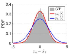
(a)

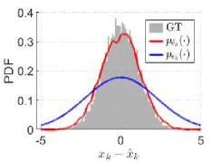
(b)

(c)

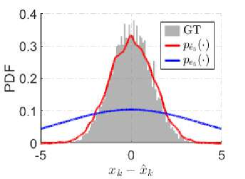
(d)

Figure 3: The approximated PDFs of the state estimation errors for $k\!=\!2,3,4,5$. The Red line denotes $\hat{p}_{\hat{e}_{k}}(\cdot)$ calculated using our proposed methods ($k=2$ using PAM and $k=3,4,5$ using PNM) and the blue line is $\hat{p}_{e_{k}}(\cdot)$ obtained from the conventional approach (CAM). The gray area represents the GT PDF using Monte Carlo sampling.

VI Experimental Study

In this section, we conduct an experimental study of a leader-follower autonomous driving scenario to validate our theoretical results interpreted so far. The leader-follower scenario is a simplified case of the widely-used platooning model in autonomous driving [35]. As illustrated in Fig. 4, the system contains a leader vehicle that maneuvers according to a certain trajectory. A follower vehicle is dedicated to keeping a constant distance from the leader vehicle. The positions and velocities of the vehicles are measured using a series of remote sensors. Both the vehicles and the sensors are connected using a common communication network that allows data exchange and state sampling. The switches installed on remote sensors, subject to the triggering scheme (5), determine whether to transmit the most recent vehicle states to the network.

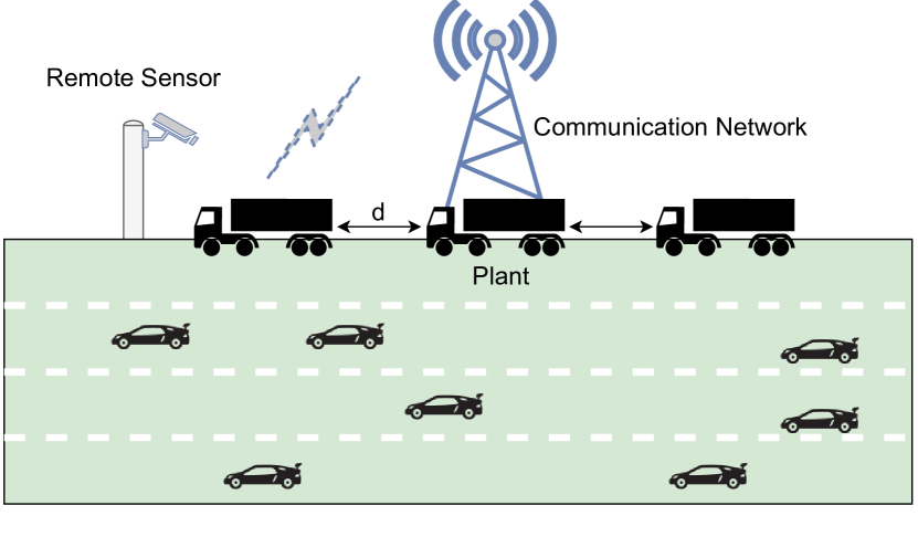
Figure 4: Illustration of a leader-follower system.

The position of the leader vehicle follows a predefined trajectory $p^{L}(t)=-\cos(t)+1.2t$. The follower is required to maintain a distance $d=3\,$m with the leader. The kinematic model of the follower vehicle is

$$\begin{split}\dot{p}(t)\,&=v(t),\quad\;\dot{v}(t)\,=u(t),\end{split}$$ (44)

where $p(t),v(t),u(t)\in\mathbb{R}$ are respectively the position, the velocity, and the acceleration of the follower. In this experiment, the parameters are selected as $\gamma=1$, $Q=1$, and $K=1$. The objective of the problem is to design a control law $u(t)$, such that $p(t)\rightarrow p^{L}(t)+d$ and $v(t)\rightarrow\dot{p}^{L}(t)$ as time $t$ increases. We define the following feedback control law,

$$\begin{split}u(t)&=-\gamma Q^{-1}v(t)-Q^{-1}Kp(t)+\gamma Q^{-1}\dot{p}^{L}(t)\\ &\leavevmode\nobreak\ \leavevmode\nobreak\ \leavevmode\nobreak\ +Q^{-1}Kp^{L}(t)+\ddot{p}^{L}(t)+Q^{-1}Kd,\end{split}$$ (45)

where $K,Q,\gamma\in\mathbb{R}^{+}$ are positive parameters. It can be verified using a Lyapunov method that $p(t)-p^{L}(t)=d$ and $v(t)-\dot{p}^{L}(t)=0$ render a globally asymptotic equilibrium of the closed-loop system, which indicates the achievement of the desired control performance. The proof is omitted in this paper.

In our experiment, we consider the discrete-time version of the follower vehicle (44),

$$\begin{split}p_{k+1}&=p_{k}+\Delta{t}v_{k},\\ v_{k+1}&=v_{k}+\Delta{t}u_{k}+w_{k},\\ \end{split}$$ (46)

where $\Delta{t}$ is the sampling period, and $w_{k}$ is an i.i.d. noise process. Accordingly, we discretize the reference trajectory $p^{L}(t)$ to $p^{L}_{k}$ using discrete sampling $t=k\cdot\Delta t$. In correspondence with the ET-SCS model in Fig. 2, the leader’s trajectory $p^{L}_{k}$ is the reference signal of the overall system. Each follower is a plant with the state $x_{k}\!=\!v_{k}$. The limited communication bandwidth motivates the application of the event-triggered scheduler in (5), for which we set $\eta\!=\!1$, and $T\!=\!20$ in this experiment. The state estimator (2) is used to obtain $\hat{x}_{k}\!=\!\hat{v}_{k}$, with $A\!=\!1$, and $B\!=\!\Delta t$. The discrete-time controller based on the estimated state is $u_{k}=u(k\cdot\Delta t)$, for which $\hat{p}_{k}$ is obtained using the recursive model $\hat{p}_{k+1}=\hat{p}_{k}+\Delta{t}\hat{v}_{k}$. The simulation runs for $10^{4}$ trials with the same initial conditions $p_{0}=0$ and $v_{0}=0$. Each trial lasts for $t=40\,s$ with a sampling time $\Delta t=0.1s$. The overall control performance is shown in Fig. 5. It is observed that the average following distance $E(p(t))-p^{L}(t)$ slightly fluctuates around $d=3\,$m, which indicates satisfactory distance keeping. Also, the average velocity $E(v(t))$ is very close to the reference velocity $\dot{p}^{L}(t)$. This shows that the configuration of the state estimator (2) and the event-triggered scheduler (5) successfully achieves the control objectives.

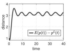
(a)

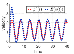
(b)

Figure 5: Average performance of the platoon controller (45). Plot (a) depicts the tracking distance $\mathsf{E}(p(t))-p^{L}(t)$. Plot (b) shows the leading velocity $\dot{p}^{L}(t)$ (in red) and the mean of the actual velocity $\mathsf{E}(v(t))$ (in blue).

The computed values of the ACR $\mathsf{E}(\delta_{k})$, using Algorithm 1 (PNM), with various triggering thresholds $\eta$, are shown in Fig. 6 (in red). To verify the validity of our proposed method, we also show the GT-ACR obtained from Monte-Carlo simulation (in black), and the ACR computed according to the conventional method (CAM), i.e., $\breve{E}(\delta_{k})$ (in blue). The information delivered by Fig. 6 can be summarized as follows.

VI-1 The general existence of the stationary ACR

It is noticed that all ACR values, $\mathsf{E}(\delta_{k})$, $\breve{\mathsf{E}}(\delta_{k})$, and the GT-ACR, ultimately converge to their respective stationary points for all triggering threshold values $\eta=1,2,3,4$. This validates our result on the existence of the stationary ACR in Sec. III-C.

VI-2 The accuracy of the proposed method

It is observed that the computed ACR $\mathsf{E}(\delta_{k})$ closely follows the GT-ACR at all time, indicating the accuracy of our proposed method. On the contrary, $\breve{\mathsf{E}}(\delta_{k})$ shows deviations from the GT-ACR suggesting inaccuracy of computing the ACR by this method. Also, $\breve{\mathsf{E}}(\delta_{k})$ is in general larger than $\mathsf{E}(\delta_{k})$ in the steady state, which validates our theoretical statement in Sec. V-A that this method overestimates the stationary ACR.

VI-3 The influence of the triggering threshold

The stationary ACR values tend to be smaller as the triggering threshold $\eta$ increases. The intuition behind this observation is that, higher threshold means higher estimation errors are tolerable, hence less events will be triggered to reset the estimation error, which consequently leads to lower ACR. Similar observation is depicted in Fig. 7, where the change of stationary ACRs $\mathsf{E}(\delta_{\infty})$ and $\breve{\mathsf{E}}(\delta_{k})$, and their ratios are plotted versus the changes of the threshold $\eta$. It van be seen that $\mathsf{E}(\delta_{\infty})<\breve{\mathsf{E}}(\delta_{k})$, for all values of $\eta$. However, the scale of the deviation between the two approaches is not monotone with respect to $\eta$, i.e., larger triggering thresholds do not necessarily lead to larger deviations . The largest deviation occurs around $\eta=3$, with more than $25\%$, which is noticeable.

(a) $\eta=1$

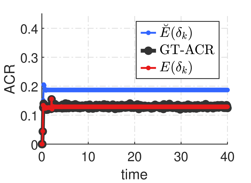
(b) $\eta=2$

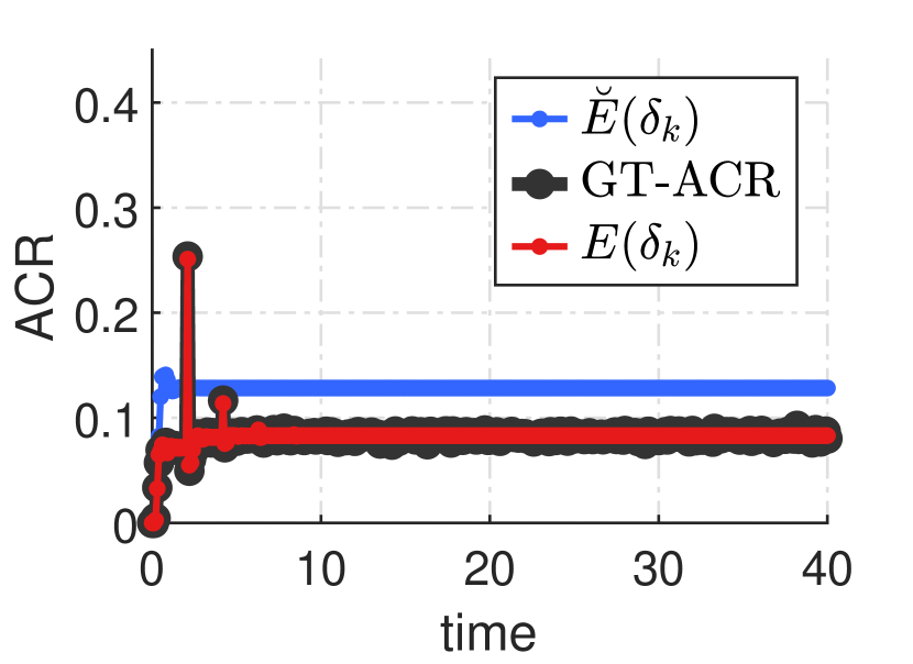
(c) $\eta=3$

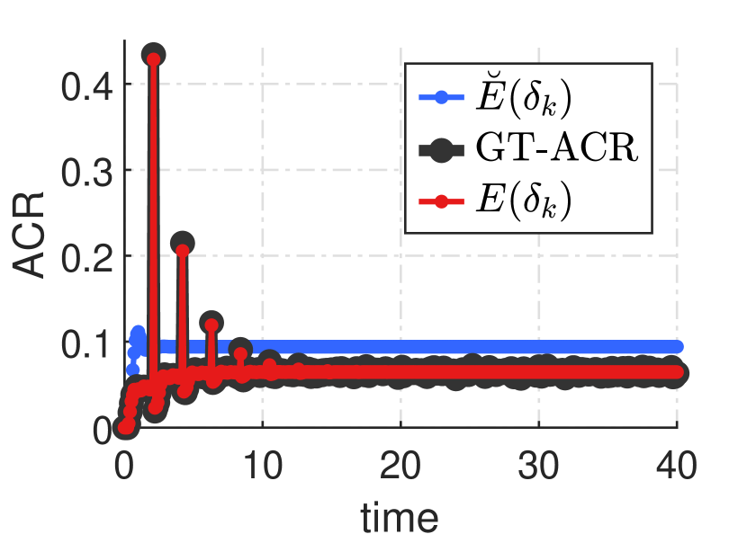
(d) $\eta=4$

Figure 6: ACRs computed using our proposed method $\mathsf{E}(\delta_{k})$ (in red), the existing method $\breve{\mathsf{E}}(\delta_{k})$ (in blue), and GT-ACR (in black), for various triggering thresholds $\eta=1,2,3,4$.

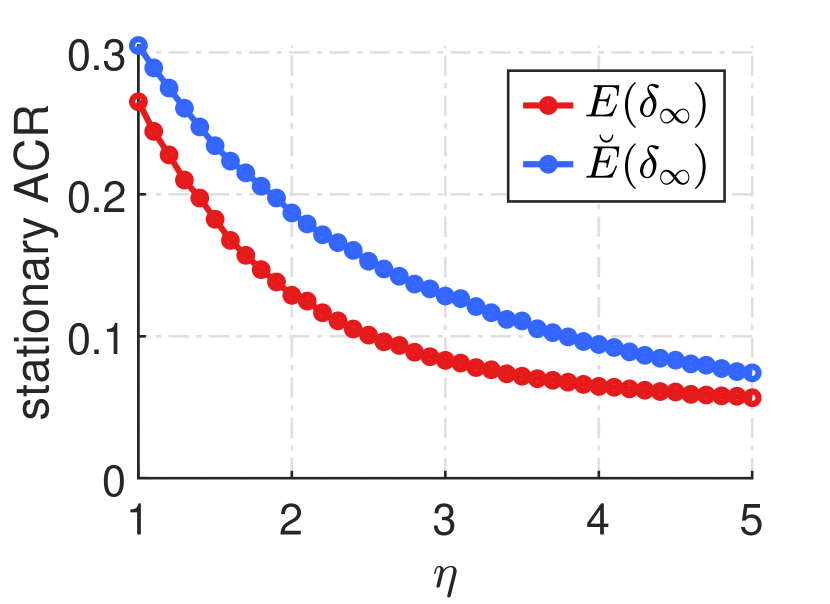
(a) Stationary ACRs

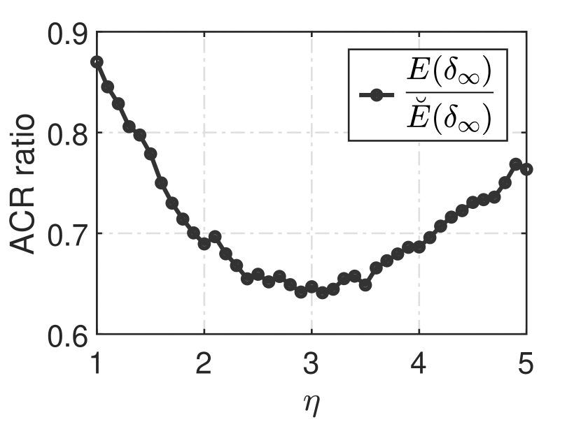
(b) ACR ratio

Figure 7: Comparison between the stationary ACRs vs. triggering threshold. Plot (a), our proposed method $\mathsf{E}(\delta_{\infty})$ (in red), and the existing method $\breve{\mathsf{E}}(\delta_{\infty})$ (in blue). Plot (b) shows the ratio of the two stationary ACRs vs. triggering threshold.

VII Conclusion

Motivated by the conservativeness of the conventional existing methods, in this article we provide comprehensive analytical formulations to accurately compute the average communication rate for networked control systems under the event-triggered sampling model. By incorporating the distribution truncation operations that correspond to the side information generated by the triggering decisions, we prove the existence of stationary ACR using a novel recursive model. Afterwards, we propose analytical and numerical approaches to accurately calculate ACR at any arbitrary time and demonstrate the noticeable ACR over-estimation when the triggering-induced truncations are ignored in computing the ACR. Our proposed method and the theoretical claims are validated with a numerical example and an experimental study on a platooning scenario, showing that our ACR computation model precisely follows the ground truth case.

References

- [1] S. Cai and V. K. Lau, “Zero MAC latency sensor networking for cyber-physical systems,” IEEE Transactions on Signal Processing, vol. 66, no. 14, pp. 3814–3823, 2018.
- [2] F. Mager, D. Baumann, R. Jacob, L. Thiele, S. Trimpe, and M. Zimmerling, “Feedback control goes wireless: Guaranteed stability over low-power multi-hop networks,” in Proceedings of the 10th ACM/IEEE International Conference on Cyber-Physical Systems, pp. 97–108, 2019.
- [3] M. Lv, D. Wang, Z. Peng, L. Liu, and H. Wang, “Event-triggered neural network control of autonomous surface vehicles over wireless network,” Science China Information Sciences, vol. 63, no. 5, pp. 1–14, 2020.
- [4] K. Astrom and B. Bernhardsson, “Comparison of riemann and lebesgue sampling for first order stochastic systems,” in Proceedings of the 41st IEEE Conference on Decision and Control, vol. 2, pp. 2011–2016, 2002.
- [5] W. P. M. H. Heemels, K. H. Johansson, and P. Tabuada, “An introduction to event-triggered and self-triggered control,” in 51st IEEE Conference on Decision and Control (CDC), pp. 3270–3285, 2012.
- [6] D. Han, Y. Mo, J. Wu, S. Weerakkody, B. Sinopoli, and L. Shi, “Stochastic event-triggered sensor schedule for remote state estimation,” IEEE Transactions on Automatic Control, vol. 60, no. 10, pp. 2661–2675, 2015.
- [7] M. H. Mamduhi, A. Molin, D. Tolić, and S. Hirche, “Error-dependent data scheduling in resource-aware multi-loop networked control systems,” Automatica, vol. 81, pp. 209–216, 2017.
- [8] R. G. Sanfelice et al., “Analysis and design of cyber-physical systems. a hybrid control systems approach,” in Cyber-physical systems: From theory to practice, pp. 1–29, CRC Press Boca Raton, FL, USA, 2016.
- [9] M. Abdelrahim, R. Postoyan, J. Daafouz, D. Nešić, and W. P. M. H. Heemels, “Co-design of output feedback laws and event-triggering conditions for thel2-stabilization of linear systems,” Automatica, vol. 87, pp. 337–344, 2018.
- [10] D. Ding, Q.-L. Han, Z. Wang, and X. Ge, “A survey on model-based distributed control and filtering for industrial cyber-physical systems,” IEEE Transactions on Industrial Informatics, vol. 15, no. 5, pp. 2483–2499, 2019.
- [11] M. Balaghiinaloo, D. J. Antunes, M. H. Mamduhi, and S. Hirche, “Decentralized LQ-consistent event-triggered control over a shared contention-based network,” IEEE Transactions on Automatic Control, vol. 67, no. 3, pp. 1430–1437, 2021.
- [12] D. Antunes and W. P. M. H. Heemels, “Rollout event-triggered control: Beyond periodic control performance,” IEEE Transactions on Automatic Control, vol. 59, no. 12, pp. 3296–3311, 2014.
- [13] B. Demirel, V. Gupta, D. E. Quevedo, and M. Johansson, “Threshold optimization of event-triggered multi-loop control systems,” in 13th International Workshop on Discrete Event Systems, pp. 203–210, 2016.
- [14] A. Molin, Optimal event-triggered control with communication constraints. PhD thesis, Technical University of Munich, 2014.
- [15] M. H. Mamduhi, A. Molin, and S. Hirche, “Event-based scheduling of multi-loop stochastic systems over shared communication channels,” in 21st International Symposium on Mathematical Theory of Networks and Systems (MTNS), 2014.
- [16] Q. Liu, M. Ye, J. Qin, and C. Yu, “Event-triggered algorithms for leader–follower consensus of networked Euler–Lagrange agents,” IEEE Transactions on Systems, Man, and Cybernetics: Systems, vol. 49, no. 7, pp. 1435–1447, 2017.
- [17] S. Ebner and S. Trimpe, “Communication rate analysis for event-based state estimation,” in 13th International Workshop on Discrete Event Systems (WODES), pp. 189–196, 2016.
- [18] A. Molin and S. Hirche, “Price-based adaptive scheduling in multi-loop control systems with resource constraints,” IEEE Transactions on Automatic Control, vol. 59, no. 12, pp. 3282–3295, 2014.
- [19] M. H. Mamduhi, J. S. Baras, K. H. Johansson, and S. Hirche, “State-dependent data queuing in shared-resource networked control systems,” in IEEE Conference on Decision and Control, pp. 1731–1737, 2018.
- [20] J. Wu, Q.-S. Jia, K. H. Johansson, and L. Shi, “Event-based sensor data scheduling: Trade-off between communication rate and estimation quality,” IEEE Transactions on Automatic Control, vol. 58, no. 4, pp. 1041–1046, 2012.
- [21] J. Wu, Y. Yuan, H. Zhang, and L. Shi, “How can online schedules improve communication and estimation tradeoff?,” IEEE Transactions on Signal Processing, vol. 61, no. 7, pp. 1625–1631, 2013.
- [22] D. Shi, T. Chen, and L. Shi, “Event-triggered maximum likelihood state estimation,” Automatica, vol. 50, no. 1, pp. 247–254, 2014.
- [23] B. Demirel, A. S. Leong, and D. E. Quevedo, “Performance analysis of event-triggered control systems with a probabilistic triggering mechanism: The scalar case,” IFAC-PapersOnLine, vol. 50, no. 1, pp. 10084–10089, 2017.
- [24] A. S. Leong, S. Dey, and D. E. Quevedo, “Sensor scheduling in variance based event triggered estimation with packet drops,” IEEE Transactions on Automatic Control, vol. 62, no. 4, pp. 1880–1895, 2016.
- [25] M. Xia, V. Gupta, and P. J. Antsaklis, “Networked state estimation over a shared communication medium,” IEEE Transactions on Automatic Control, vol. 62, no. 4, pp. 1729–1741, 2016.
- [26] A. Mohammadi and K. N. Plataniotis, “Event-based estimation with information-based triggering and adaptive update,” IEEE Transactions on Signal Processing, vol. 65, no. 18, pp. 4924–4939, 2017.
- [27] L. Zou, Z. Wang, Q.-L. Han, and D. Zhou, “Recursive filtering for time-varying systems with random access protocol,” IEEE Transactions on Automatic Control, vol. 64, no. 2, pp. 720–727, 2018.
- [28] V. S. Dolk, J. Ploeg, and W. P. M. H. Heemels, “Event-triggered control for string-stable vehicle platooning,” IEEE Transactions on Intelligent Transportation Systems, vol. 18, no. 12, pp. 3486–3500, 2017.
- [29] B. Liu, D. Jia, K. Lu, D. Ngoduy, J. Wang, and L. Wu, “A joint control–communication design for reliable vehicle platooning in hybrid traffic,” IEEE Transactions on Vehicular Technology, vol. 66, no. 10, pp. 9394–9409, 2017.
- [30] L. Dong, Y. Tang, H. He, and C. Sun, “An event-triggered approach for load frequency control with supplementary ADP,” IEEE Transactions on Power Systems, vol. 32, no. 1, pp. 581–589, 2016.
- [31] S. Saxena and E. Fridman, “Event-triggered load frequency control via switching approach,” IEEE Transactions on Power Systems, vol. 35, no. 6, pp. 4484–4494, 2020.
- [32] P. B. g. Dohmann and S. Hirche, “Distributed control for cooperative manipulation with event-triggered communication,” IEEE Transactions on Robotics, vol. 36, no. 4, pp. 1038–1052, 2020.
- [33] V.-T. Ngo and Y.-C. Liu, “Event-based communication and control for task-space consensus of networked Euler–Lagrange systems,” IEEE Transactions on Control of Network Systems, vol. 8, no. 2, pp. 555–565, 2021.
- [34] E. I. Jury, Theory and Application of the z-Transform Method. Wiley, 1964.
- [35] A. Liu, L. Lian, V. Lau, G. Liu, and M.-J. Zhao, “Cloud-assisted cooperative localization for vehicle platoons: A turbo approach,” IEEE Transactions on Signal Processing, vol. 68, pp. 605–620, 2020.