LVRNet: Lightweight Image Restoration for
Aerial Images under Low Visibility

Abstract

Learning to recover clear images from images having a combination of degrading factors is a challenging task. That being said, autonomous surveillance in low visibility conditions caused by high pollution/smoke, poor air quality index, low light, atmospheric scattering, and haze during a blizzard becomes even more important to prevent accidents. It is thus crucial to form a solution that can result in a high-quality image and is efficient enough to be deployed for everyday use. However, the lack of proper datasets available to tackle this task limits the performance of the previous methods proposed. To this end, we generate the LowVis-AFO dataset, containing 3647 paired dark-hazy and clear images. We also introduce a lightweight deep learning model called Low-Visibility Restoration Network (LVRNet). It outperforms previous image restoration methods with low latency, achieving a PSNR value of 25.744 and an SSIM of 0.905, making our approach scalable and ready for practical use. The code and data can be found here.

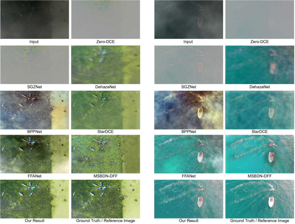
Figure 1: Visual results on the proposed LowVis-AFO dataset. The method used to obtain each result has been mentioned under the image.

1 Introduction

Image enhancement and restoration have been a critical area of research using both traditional digital image processing techniques[12] [2], and the recent deep learning frameworks[32][33][44]. The goal of image restoration is to recover a clear image, whereas image enhancement is to improve the quality of the degraded image. In this study, we perform recovery of the clear image from the hazy version while performing low-light image enhancement using a single convolutional network, which could further be applied to tasks such as search and rescue operations using object detection.

Using deep learning algorithms for image recovery has many benefits, the most important being that it can generalize to different variations in the images captured. Hence, we observe that deep learning-based methods on most benchmark datasets often outperform traditional methods significantly. However, there are still challenges that the researchers have to tackle for image restoration. Publicly available datasets containing a variety of degrading factors that model real-world scenarios are few. Hence, most previous works have focused on removing one type of degradation with a specific intensity level. From the perspective of computational complexity, recent deep learning methods are computationally expensive, and thus they can’t be deployed on edge devices. Moreover, image restoration has been a long-standing ill-posed research problem, as there are infinite mappings between the degraded and the clear image. Thus, the existing methods still have room for improvement in finding the correct mapping.

In this work, we focus on developing an end-to-end lightweight deep-learning solution for the image restoration task. Our major contributions are listed below:

• Taking inspiration from Non-linear Activation Free Network (NAFNet) [5] and Level Attention Module [45], we propose a novel algorithm - Low-Visibility Restoration Network (LVRNet), that can effectively recover high-quality images from degraded images taken in poor visual conditions (Figure 1).

• Due to the lack of available datasets that exhibit a combination of adverse effects, we generate a new dataset, namely LowVis-AFO (abbreviation for Low-Visibility Aerial Floating Objects dataset). We use AFO [15] as our ground truth dataset and synthesize dark hazy images. The data generation process has been elaborated in Section 4.1.

• Benchmarking experiments have been provided on the LowVis-AFO dataset to help future researchers for quantitative comparison. Along with that, LVRNet surpasses the results obtained using previous image restoration techniques by a significant margin.

• We perform extensive ablation studies to analyze the importance of various loss functions existing in current image restoration research. These experiments are discussed in detail in Section  5.

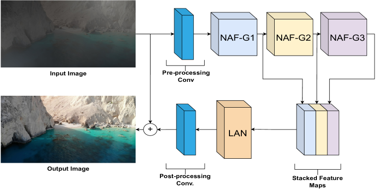
Figure 2: Model architecture of the proposed LVRNet. Starting from the top-left: The input image is passed to the pre-processing convolution layers where feature maps are learned and passed to NAF Groups (here we have used 3 groups). The features extracted from each group are concatenated (or stacked) along the channel dimension and sent as input to the Level Attention Module (LAM). Finally, we pass LAM’s output to CNN layers for post-processing, adding the original image through residual connection and extracting the restored image at the bottom-left.

2 Related Works

This section highlights the previous work done in the fields of image dehazing and low-light image enhancement and their limitations.

2.1 Image Dehazing

Hazy weather is often seen due to floating particles in the environment which degrade the quality of the image captured. Therefore, many previous works have tried to recover a clear image from the hazy one. These works can be divided into two methods, ones that rely on prior assumptions [17] and the atmospheric scattering model (ASM) [31] and the others which use deep learning to solve the problem, either by combination with ASM [3][34][36] or independently [25][26][33][46][50]. Conventional approaches are physically inspired and apply various types of sharp image priors to regularize the solution space. However, they exhibit shortcomings when implemented with real-world images and videos. For example, the dark channel prior method (DCP) [31] does not perform well in regions containing the sky. These methods [1][11][24] are known to be computationally expensive and require heuristic parameter-tuning. Supervised dehazing methods can be divided into two subparts, one is ASM based, and the other is non-ASM based.

ASM-based Learning: MSCNN[34] solves the task of image dehazing by dividing the problem into three steps: using CNN to estimate the transmission map $t(x)$, using statistical methods to find atmospheric light $A$ and then recover the clear image $J(x)$ using $t(x)$ and $A$ jointly. Methods like LAP-Net [23] adopt the relation of depth with the amount of haze in the image. The farther the scene from the camera, the denser the haze would be. Hence it considers the difference in the haze density in the input image using a stage-wise loss, where each stage predicts the transmission map from mild to severe haze scenes. DehazeNet [3] consists of four sequential operations: feature extraction, multi-scale mapping, calculating local extremum, and non-linear regression. MSRL-DehazeNet [43] decomposes the problem into recovering high-frequency and basic components. GCANet [4] employs residual learning between haze-free and hazy images as an optimization objective.

End-to-end Learning: This subpart of previous work corresponds to non-ASM-based deep learning methods for recovering the clear image. Back-Projected Pyramid Network (BPPNet) [39] is a generative adversarial network that includes iterative blocks of UNets [37] to learn haze features and pyramid convolution to preserve spatial features of different scales. The reason behind using iterative blocks of UNets[37] is to avoid increasing the number of encoder layers in a single UNet[37] as it leads to a decrease in height and width of latent feature representation hence resulting in loss of spatial information. Moreover, different blocks of UNet learn different complexities of haze features, and the final concatenation step ensures that all of them are taken into account during image reconstruction. The final reconstruction is done using the pyramid convolution block. The output feature is post-processed to get a haze-free image. Feature-Fusion Attention Network (FFANet) [33] adopts the idea of an attention mechanism and skip connections to restore haze-free images. A combination of channel attention and pixel attention is introduced, which helps the network, deal with the uneven spatial distribution of haze and different weighted information across channels. Autoencoders [6], hierarchical networks [9], and dense block networks [14] has also been proposed for the task of image dehazing. However, our main comparison lies with FFANet [33], wherein we show a huge improvement compared to the former method with a model containing a lesser number of parameters and which can generalize to different levels of haze.

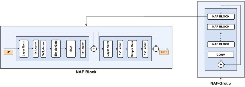
Figure 3: Architecture of NAF Block and NAF Group. NAF Blocks are the building blocks of NAF Groups. A detailed description has been provided in Section 3.1 and Section 3.1.1

2.2 Low-light Enhancement

Traditional methods for low-light image enhancement (LLIE) include Histogram Equalization-based methods and Retinex model-based methods. Recent research has been focused on developing deep learning-based methods following the success of the first seminal work. Deep learning-based solutions are more accurate, robust, and have a shorter inference time thus attracting more researchers. Learning strategies used in these methods are mainly supervised learning [27, 29, 30, 35, 51, 28, 41], unsupervised learning [20], and zero-shot learning [49, 13].
Supervised Learning: The first deep learning-based LLIE method LLNet [27] is an end-to-end network that employs a variant of stacked-sparse denoising autoencoder to brighten and denoise low-light images simultaneously. LLNet inspired many other works [29, 30, 35, 51], but they do not consider the observation that noise exhibits different levels of contrast in different frequency layers. Later, Xu et al. [41] proposed a network that suppresses noise in the low-frequency layers and recovers the image contents by inferring the details in high-frequency layers. There is another division of methods that is based on the Retinex theory. Deep Retinex-based models [40, 42] decomposes the image into two separate components - light-independent reflectance and structure-aware smooth illumination. The final estimated reflection component is treated as the enhanced result.
Unsupervised Learning: Although the above-mentioned methods perform well on synthetic data, they show limited generalization capability on real-world low-light images. This might be the result of overfitting. EnlightenGAN [20] proposed to solve this issue by adopting an unsupervised learning technique, i.e., avoiding the use of paired synthetic data. This work uses attention-guided UNet as a generator and global-local discriminators to achieve the objective of LLIE.
Zero-short Learning: These methods, in low-level vision tasks, do not require any paired or unpaired training data. Zero-reference Deep Curve Estimation [13] formulates image enhancement as a task of image-specific deep curve estimation, taking into account pixel value range, monotonicity, and differentiability. It is a lightweight DCE-Net that doesn’t require paired or unpaired ground truth images during training and relies on non-reference loss functions that measure the enhancement quality hence driving the learning of the network. Another such method, Semantic-guided Zero-shot low-light enhancement Network [49] is a lightweight model for low-light enhancement factor extraction which is inspired by the architecture of U-Net [37]. The output of this network is fed to a recurrent image enhancement network, along with the degraded input image. Each stage in this network considers the enhancement factor and the output from the previous scale as its input. This is followed by a feature-pyramid network that aims to preserve the semantic information in the image.

More recently, researchers have experimented with transformers for Zero-shot Learning LLIE. Structure-Aware lightweight Transformer (STAR) [47] focuses on real-time image enhancement without using deep-stacked CNNs or large transformer models. STAR is formulated to capture long-range dependencies between separate image patches, facilitating the model to learn structural relationships between different regions of the images. In STAR, patches of the image are tokenized into token embeddings. The tokens generated as an intermediate stage are passed to a long-short-range transformer that outputs two long and short-range structural maps. These structural maps can further predict curve estimation or transformation for image enhancement tasks. Although these methods show impressive results for the study of low-light image enhancement for which it originally developed, they cannot deal with foggy low– light images.

2.3 Limitations

Previous works have relied on ASM-based methods in the case of dehazing and Retinex model-based methods for low-light image enhancement. However, these methods fail to generalize to real-world images. Recent deep learning-based methods using large networks solve the task of image dehazing and low-light enhancement separately. To our knowledge, no work is introduced that solves the two problems in a collaborative network. Deep learning methods also fail to generalize to different haze levels and darkness.

3 Proposed Methodology

In this section, we provide a detailed description of the overall architecture proposed and the individual components included in the network.

3.1 Architecture

Like the group structure in [33], each group in our network consists of a $K$ NAF Block [5] with a skip connection at the end as shown in Figure 3. The output of each group is concatenated, passed to the level attention module to find the weighted importance of the feature maps obtained, and post-processed using two convolutional layers. A long skip connection for global residual learning accompanies this.

3.1.1 NAF-Block

To keep this work self-contained, we explain the NAF Block [5] in this subsection. NAF Block is the building block of Nonlinear Activation Free Network. Namely NAFNet [5]. To avoid over-complexity in the architecture, this block avoids using any activation functions like ReLU, GELU, Softmax, etc. hence keeping a check on the intra-block complexity of the network.

The input first passes through Layer Normalization as it can help stabilize the training process. This is followed by convolution operations and a Simple Gate (SG). SG is a variant of Gated Linear Units (GLU) [10] as evident from the following equations 1 and 2

$$GLU(X,f,g,\sigma)=f(X)\odot\sigma(g(X))$$ (1)

$$SimpleGate(X,Y)=X\odot Y$$ (2)

and a replacement for GELU[18] activation function because of the similarity between GLU and GELU (Equation 3).

$$GELU(x)=x\phi(x)$$ (3)

In Simple Gate, the feature maps are divided into two parts along the channel dimension and then multiplied as shown in Figure 4. Another novelty introduced in this block is Simplified Channel Attention (SCA). Channel Attention (CA) can be expressed as:

$$CA(X)=X\otimes\sigma(W_{2}max(0,W_{1}pool(X)))$$ (4)

where $X$ represents the feature map, $pool$ indicates the global average pooling operation,$\sigma$ is Sigmoid, $W1,W2$ are fully-connected layers and $\otimes$ is a channel-wise product operation. This can be taken as a special case of GLU from which we can derivate the equation for Simplified Channel Attention:

$$SCA(X)=X\otimes Wpool(X)$$ (5)

3.1.2 Level Attention Module

Once we have extracted features from all the NAF Groups, we concatenate them and pass them through the Level Attention Module (LAM) [45]. This module learns attention weights for features obtained at different levels.

In LAM, each feature map is first reshaped to a 2D matrix of the size $K\times HWC$, where $K,H,W,$ and $C$ are the no. of NAF Groups, height, width, and no. of channels of the feature maps respectively. We find a correlation matrix of this 2D matrix by multiplying it with its transpose matrix. Finally, we multiply the 2D matrix with this correlation matrix and reshape it to $K\times H\times W\times C$ tensor. Inspired by residual learning, this tensor is substituted for residual and is added to the original concatenated feature maps. The resultant features are then reshaped to $H\times W\times KC$, passing through $1\times 1$ convolution operation to get the $H\times W\times C$ feature map. This is passed through some post-processing convolutions to get the final enhanced output. We include its architecture diagram in the supplementary material for a better understanding.

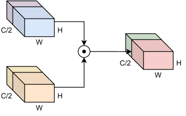
Figure 4: Simple Gate as represented by Equation 2 $\otimes$ denotes channel-wise multiplicaWere

3.2 Loss Functions

Four loss functions, namely, reconstruction loss, perceptual loss, edge loss [19], and FFT loss[7], have been used to supervise the task of image restoration.

The total loss L is defined in Equation 6, where $\lambda_{1}=0.04$, $\lambda_{2}=1$ and $\lambda_{3}=0.01$.

$$L=L_{s}+\lambda_{1}L_{p}+\lambda_{2}L_{e}+\lambda_{3}L_{f}$$ (6)

3.2.1 Reconstruction Loss:

The restored clear output image is compared with its ground truth value in the spatial domain using a standard $l_{1}$ loss as demonstrated in Equation 7. We use $l_{1}$ loss instead of $l_{2}$ loss as it does not over-penalize the errors and leads to better image restoration performance [48].

$$L_{s}=\frac{1}{N}\sum\limits_{i=1}^{n}\parallel x_{i}^{gt}-NAFNet(x_{i}^{dark,hazy})\parallel_{1}$$ (7)

In the above equation, $x_{i}^{gt}$ refers to the ground truth clear image, and $NAFNet(x_{i}^{dark,hazy})$ denotes the output of our proposed NAFNet when a dark and hazy image is fed to the network.

3.2.2 Perceptual Loss:

To reduce the perceptual loss and improve the image’s visual quality, we utilize the features of the pre-trained VGG-19 network [38] obtained from the output of one of the ReLU activation layers. It is defined in Equation 8, where $w_{ij}$, $h_{ij}$, and $c_{ij}$ refer to the dimensions of the respective feature maps inside the VGG-19 architecture. $\phi_{ij}$ denotes the feature maps outputted from the jth convolutional layer inside the i-th block in the VGG network.

$$L_{p}=\frac{1}{w_{ij}h_{ij}c_{ij}}\sum\limits_{x=1}^{w_{ij}}\sum\limits_{y=1}^{h_{ij}}\sum\limits_{z=1}^{c_{ij}}\parallel\phi_{ij}(I_{gt})_{xyz}-\phi_{ij}(I_{out})_{xyz}\parallel$$ (8)

3.2.3 Edge Loss:

To recover the high-frequency details lost because of the inherent noise in dark and hazy images, we have an additional edge loss to constrain the high-frequency components between the ground truth and the recovered image.

$$L_{e}=\sqrt{(\nabla^{2}(I_{gt})-\nabla^{2}(I_{out}))^{2}+\epsilon^{2}}$$ (9)

In Equation 9, $\nabla^{2}$ refers to the Laplacian operation [22], which is then applied to the ground truth and the predicted clean image to get the edge loss.

3.2.4 FFT Loss:

To supervise the haze-free results in the frequency domain, we add another loss called Fast Fourier transform (FFT) loss (denoted by $L_{f}$ in Equation 12. It calculates the loss of both amplitude and phase using the $l_{1}$ loss function without additional inference cost.

$$A_{x_{i}^{gt}},P_{x_{i}^{gt}}=FFT(x_{i}^{gt}),$$ (10)

$$A_{x_{i}^{out}},P_{x_{i}^{out}}=FFT(x_{i}^{out}),$$ (11)

$$L_{f}=\frac{1}{N}\sum\limits_{i=1}^{n}(\parallel A_{x_{i}^{gt}}-A_{x_{i}^{out}}\parallel_{1}+\parallel P_{x_{i}^{gt}}-P_{x_{i}^{out}}\parallel_{1})$$ (12)

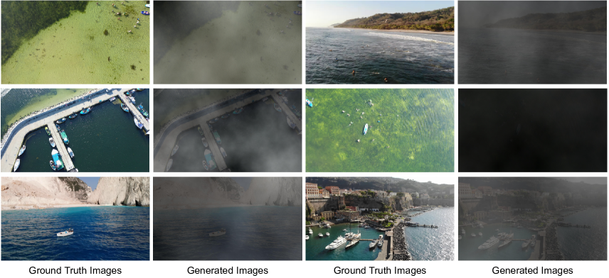
Figure 5: Visual illustration of a few sample images from our dataset. Columns 1 and 3 show original images taken from AFO Dataset [15], whereas Columns 2 and 4 show their corresponding images generated as explained in Section 4.1 simulating low-visibility conditions.

4 Experimental Results

To demonstrate the outcomes of our model’s approach towards image enhancement under low-visibility conditions, this section contains a detailed description of the dataset generated and used in Section 4.1, the experimental settings in Section 4.2, the metrics used for evaluation in Section 4.3 and a discussion on the results obtained in Section 5.1 and 5.2.

4.1 Dataset Details

Due to the lack of available datasets that meet our requirements, we generate a new one using the AFO dataset [15]. The dataset generation process has been elaborated below, and the final images have been shown in Figure 5.

• Haze effect - To add fog, imgaug [21], a well-known python library was used. A random integral value between 3, 4, 5 was selected, representing the fog’s severity. For each image, this random number was chosen and pre-defined functions within the package were utilized to add a layer of fog to the image.

• Low-light Effect - Given a normal image, our goal is to output a low-lit image while preserving the underlying information. We follow the pipeline introduced [8], which parametrically models the low light-degrading transformation by observing the image signal processing (ISP) pipeline between the sensor measurement system and the final image. The low-illumination-degrading pipeline is a three-stage process:

  • Unprocessing procedure - This part aims to synthesize RAW format images from input sRGB images by invert tone mapping, invert gamma correction, and the transformation of the image from sRGB space to cRGB space, and invert white balancing.

  • Low Light Corruption - This aims at adding shot and read noises to the output of the unprocessing procedure, as these are common in-camera imaging systems. Shot noise is a type of noise generated by the random arrival of photons in a camera, which is a fundamental limitation. Read noise occurs during the charge conversion of electrons into voltage in the output amplifier, which can be approximated using a Gaussian random variable with zero mean and fixed variance.

  • ISP Pipeline - RAW image processing is done after the lowlight corruption process in the following order: add quantization noise, white balancing from cRGB to sRGB, and gamma correction, which finally outputs a degraded low-light image.

• Combination of Haze and Low-light Effect - Results of implementing the low-light generation algorithm described above on foggy images generated using img-aug are shown here. It can be seen that combining the two (fog and low light) has introduced adversity in finding the location of the objects in the water bodies. Moreover, finding a unique solution for such a combination has not been explored to date

4.2 Experimental Settings

The images were resized to get the resultant dimensions as $256\times 456$. Adam optimizer with an initial learning rate of $1e\scalebox{0.75}[1.0]{$-$}4$, $\beta_{1}$, and $\beta_{2}$ with a value of 0.9 and 0.999 were chosen. The batch size was fixed as 2. We have used 3 groups in all our experiments, each with 16 blocks. Pytorch backend was used to compile the model and train it.

4.3 Evaluation Metrics

We reported the results we obtained using two standard image restoration metrics (i.e., PSNR and SSIM). These metrics will help us quantitatively evaluate the performance of our model in terms of feature colors and structure similarity. High PSNR and SSIM values if indicative of good results.

5 Experimental Results

The architecture used is given in Figure 2. This section gives a detailed analysis of the results obtained by the proposed method.

Method	Year	PSNR	SSIM
Zero-DCE[13]	$2020$	$12.323$	$0.529$
SGZNet[49]	$2022$	$12.578$	$0.519$
BPPNet[39]	$2022$	$15.507$	$0.755$
DehazeNet[3]	$2016$	$15.710$	$0.391$
Star-DCE[47]	$2021$	$16.651$	$0.539$
FFANet[7]	$2020$	$15.050$	$0.582$
MSBDN-DFF[16]	$2020$	$16.686$	$0.689$
LVRNet (Ours)	$2022$	$25.744$	$0.905$

Table 1: Quantitative comparison of our proposed network with previous work. The best results and the second-best results have been highlighted with red color and blue colors, respectively.

S.no.	Reconstruction Loss	Perceptual Loss	Edge Loss	FFT Loss	PSNR	SSIM
1.	✓	✓	✗	✗	24.070	0.870
2.	✓	✓	✗	✓	25.455	0.903
3.	✓	✓	✓	✗	25.624	0.897
4.	✓	✗	✓	✓	25.719	0.900
5.	✓	✓	✓	✓	25.744	0.905

Table 2: Ablation experiments: We train our model using different combinations of loss functions to understand the importance of individual losses for image restoration. The best results are obtained when the model is trained using all the loss functions mentioned in this work.

5.1 Discussion and Comparison

In this subsection, we discuss the evaluation results obtained by the proposed pipeline. Previous methods were trained on the newly generated dataset and tested to compare their metrics with our model’s performance. These methods were built to enhance the low-light image or obtain a clear image from a hazy one. The results are mentioned in Table 1.

We observe a huge increase in the PSNR value as compared to Zero-DCE[13], which enhances the low-light image as a curve estimation problem. However, it introduces an even amplified noise leading to color degradation as seen in Figure 1. Notwithstanding its fast processing speed, Zero-DCE has limited noise suppression and haze removal capacity. Star-DCE[47], which uses a transformer backbone instead of a CNN one in the Zero-DCE network, shows a 35.12% increase in PSNR value. Owing to the added LAM structure, using which our model can focus on more important feature maps, we can achieve a 54% higher PSNR value.

SGZNet[49] uses pretrained networks for enhancement factor estimation, thus their result is dependent on those pretrained weights, leading to a lower PSNR value of 12.578 on LowVis-AFO. From Figure 1, we observe that the result obtained from SGZNet is still degraded by excessive noise and lacks saturation. DehazeNet[3] is limited by the network’s depth and cannot generalize to real-world scenarios. Hence, it results in a low PSNR of 15.710. Methods like BPPNet[39] and FFANet[33] are end-to-end deep learning methods for image dehazing. BPPNet[39] distorts the color distribution in the recovered image as it cannot remove the dark regions, whereas FFA-Net[33] produces image with a lower perceptual quality.

We propose an end-to-end deep learning pipeline (0.43M parameters) that can perform image dehazing and low-light image enhancement with a significant decrease in the number of parameters as compared to MSBDN-DFF [16] (31M parameters) and FFA-Net[33] (4.45M parameters).

The supplementary material has provided a discussion on the number of parameters of other models. We also trained the model for 10 epochs with fewer NAF blocks to prove that we achieved better results than the lighter results, not due to an increase in parameters but because of the self-sufficiency of the added LAM module, non-linear activation networks, and residual connections. The results of these experiments are reported in the supplementary material.

5.2 Ablation Studies

To prove the importance of the perceptual loss, edge loss, and fft-loss, added to supervise the training procedure, we conducted experiments excluding each of them and reported the values of PSNR and SSIM in Table 2. We keep the $l_{1}$ loss function constant in all experiments as it is critical in image restoration tasks. We observe an increase in metric values in the lower rows compared to row 1. As a result of more supervision in the unchanged architecture, there is an increase in the quality of clear images obtained, which are demonstrated in the supplementary material. There is also an increase in PSNR value (which depends on per-pixel distance) in row 3, once we train the model without perceptual loss. This is seen as perceptual loss doesn’t compare individual pixel values but the high-level features obtained from a pretrained network. In row 4, we get a lower PSNR value on excluding edge loss compared to row 5, as we get lesser edge supervision. Overall, we get the best performance when we include all the loss functions, as seen in row 5.

6 Conclusion

In this work, we have presented Low-Visibility Restoration Network (LVRNet), a new lightweight deep learning architecture for image restoration. We also introduce a new dataset, LowVis-AFO, that includes a diverse combination of synthetic darkness and haze. We also performed benchmarking experiments on our generated dataset and surpassed the results obtained using the previous image restoration network by a significant margin. Qualitative and quantitative comparison with previous work has demonstrated the effectiveness of LVRNet. We believe our work will motivate more research, focused on dealing with a combination of adverse effects such as haze, rain, snowfall, etc. rather than considering a single factor. In our future work, we plan to extend LVRNet for image restoration tasks where more factors, that negatively impact the image quality, are taken into account.

Supplementary Material

To make our submission self-contained and given the page limitation, this supplementary material provides additional details. Section 1 gives an overview of the number of parameters and PSNR obtained by different methods. Section 2 contains visual results that highlight the significance of the loss functions. Section 3 contains the ablation experiment with lesser blocks, and Section 4 demonstrates the architecture diagram of the level attention module.

1 PSNR vs Parameters

Figure 6 presents the PSNR vs. Parameters plot that the previous methods and our method achieved on the testing set of LowVis-AFO. Our model outperforms the state-of-the-art image dehazing and low-light image enhancement methods by a good margin while having a lesser number of parameters.

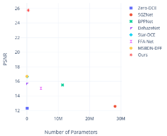
Figure 6: The PSNR vs Number of Parameters of recent image restoration methods on the newly proposed LowVis-AFO dataset.

S.no.	#Blocks	PSNR	SSIM	#params	Runtime(s)
1.	14	21.3432	0.8626	0.38M	0.035
2.	12	20.4302	0.8488	0.33M	0.029
3.	10	20.2965	0.8494	0.28M	0.024

Table 3: Results of the experiments conducted on a lesser number of NAF blocks. The training was done for 10 epochs and the metrics were obtained on the test set thereafter.

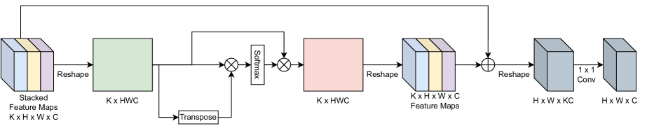
Figure 7: Visual illustration of operations performed by Level Attention Module.

2 Ablation Experiment on Different Loss Functions

Figure 8 demonstrates the visual results obtained when we conducted experiments excluding some loss functions. The motivation behind the experiment is to highlight the importance of the extra loss functions (perceptual loss, edge loss, fft-loss) added to supervise our pipeline. The quantitative results are given in Table 2 in the main manuscript.

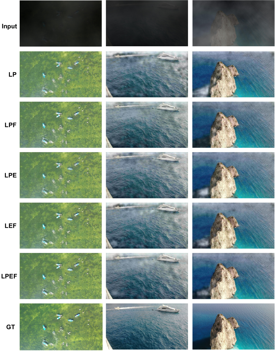
Figure 8: Qualitative results obtained from experiments conducted on different loss functions. In the figure, L = L1 loss, P = Perceptual Loss, E = Edge loss and F = FFT loss.

3 Ablation Experiment with Lesser Number of Blocks

To prove the self-sufficiency of the individual components included in our architecture such as LAM, we conduct experiments with a lesser number of NAF blocks [5] and reported the PSNR and SSIM obtained in Table 1. Seeing the results, we can conclude that our model achieves better results, not because of an increase in the number of parameters as compared to the lighter model, but because of the entire pipeline adopted.

4 Level Attention Module

As mentioned in the main text, the diagram for LAM[45] has been provided here in the supplementary material. (refer Figure 7)

References

- [1] Codruta O Ancuti, Cosmin Ancuti, Chris Hermans, and Philippe Bekaert. A fast semi-inverse approach to detect and remove the haze from a single image. In Asian Conference on Computer Vision, pages 501–514. Springer, 2010.
- [2] Julian Besag, Jeremy York, and Annie Mollié. Bayesian image restoration, with two applications in spatial statistics. Annals of the institute of statistical mathematics, 43(1):1–20, 1991.
- [3] Bolun Cai, Xiangmin Xu, Kui Jia, Chunmei Qing, and Dacheng Tao. Dehazenet: An end-to-end system for single image haze removal. IEEE Transactions on Image Processing, 25(11):5187–5198, 2016.
- [4] Dongdong Chen, Mingming He, Qingnan Fan, Jing Liao, Liheng Zhang, Dongdong Hou, Lu Yuan, and Gang Hua. Gated context aggregation network for image dehazing and deraining. In 2019 IEEE winter conference on applications of computer vision (WACV), pages 1375–1383. IEEE, 2019.
- [5] Liangyu Chen, Xiaojie Chu, Xiangyu Zhang, and Jian Sun. Simple baselines for image restoration. arXiv preprint arXiv:2204.04676, 2022.
- [6] Rongsen Chen and Edmund M-K Lai. Convolutional autoencoder for single image dehazing. In ICIP, pages 4464–4468, 2019.
- [7] Sung-Jin Cho, Seo-Won Ji, Jun-Pyo Hong, Seung-Won Jung, and Sung-Jea Ko. Rethinking coarse-to-fine approach in single image deblurring. In Proceedings of the IEEE/CVF international conference on computer vision, pages 4641–4650, 2021.
- [8] Ziteng Cui, Guo-Jun Qi, Lin Gu, Shaodi You, Zenghui Zhang, and Tatsuya Harada. Multitask aet with orthogonal tangent regularity for dark object detection. In Proceedings of the IEEE/CVF International Conference on Computer Vision, pages 2553–2562, 2021.
- [9] Sourya Dipta Das and Saikat Dutta. Fast deep multi-patch hierarchical network for nonhomogeneous image dehazing. In Proceedings of the IEEE/CVF Conference on Computer Vision and Pattern Recognition Workshops, pages 482–483, 2020.
- [10] Yann N Dauphin, Angela Fan, Michael Auli, and David Grangier. Language modeling with gated convolutional networks. In International conference on machine learning, pages 933–941. PMLR, 2017.
- [11] Raanan Fattal. Dehazing using color-lines. ACM transactions on graphics (TOG), 34(1):1–14, 2014.
- [12] Stuart Geman and Donald Geman. Stochastic relaxation, gibbs distributions, and the bayesian restoration of images. IEEE Transactions on pattern analysis and machine intelligence, (6):721–741, 1984.
- [13] Chunle Guo, Chongyi Li, Jichang Guo, Chen Change Loy, Junhui Hou, Sam Kwong, and Runmin Cong. Zero-reference deep curve estimation for low-light image enhancement. In Proceedings of the IEEE/CVF Conference on Computer Vision and Pattern Recognition, pages 1780–1789, 2020.
- [14] Tiantong Guo, Venkateswararao Cherukuri, and Vishal Monga. Dense123’color enhancement dehazing network. In Proceedings of the IEEE/CVF Conference on Computer Vision and Pattern Recognition Workshops, pages 0–0, 2019.
- [15] Jan Gąsienica-Józkowy, Mateusz Knapik, and Boguslaw Cyganek. An ensemble deep learning method with optimized weights for drone-based water rescue and surveillance. Integrated Computer-Aided Engineering, pages 1–15, 01 2021.
- [16] Dong Hang, Pan Jinshan, Hu Zhe, Lei Xiang, Zhang Xinyi, Wang Fei, and Yang Ming-Hsuan. Multi-scale boosted dehazing network with dense feature fusion. In CVPR, 2020.
- [17] Kaiming He, Jian Sun, and Xiaoou Tang. Single image haze removal using dark channel prior. IEEE transactions on pattern analysis and machine intelligence, 33(12):2341–2353, 2010.
- [18] Dan Hendrycks and Kevin Gimpel. Gaussian error linear units (gelus). arXiv preprint arXiv:1606.08415, 2016.
- [19] Kui Jiang, Zhongyuan Wang, Peng Yi, Chen Chen, Baojin Huang, Yimin Luo, Jiayi Ma, and Junjun Jiang. Multi-scale progressive fusion network for single image deraining. In Proceedings of the IEEE/CVF conference on computer vision and pattern recognition, pages 8346–8355, 2020.
- [20] Yifan Jiang, Xinyu Gong, Ding Liu, Yu Cheng, Chen Fang, Xiaohui Shen, Jianchao Yang, Pan Zhou, and Zhangyang Wang. Enlightengan: Deep light enhancement without paired supervision. IEEE Transactions on Image Processing, 30:2340–2349, 2021.
- [21] Alexander B. Jung, Kentaro Wada, Jon Crall, Satoshi Tanaka, Jake Graving, Christoph Reinders, Sarthak Yadav, Joy Banerjee, Gábor Vecsei, Adam Kraft, Zheng Rui, Jirka Borovec, Christian Vallentin, Semen Zhydenko, Kilian Pfeiffer, Ben Cook, Ismael Fernández, François-Michel De Rainville, Chi-Hung Weng, Abner Ayala-Acevedo, Raphael Meudec, Matias Laporte, et al. imgaug. https://github.com/aleju/imgaug, 2020. Online; accessed 01-Feb-2020.
- [22] Behzad Kamgar-Parsi and Azriel Rosenfeld. Optimally isotropic laplacian operator. IEEE Transactions on Image Processing, 8(10):1467–1472, 1999.
- [23] Yunan Li, Qiguang Miao, Wanli Ouyang, Zhenxin Ma, Huijuan Fang, Chao Dong, and Yining Quan. Lap-net: Level-aware progressive network for image dehazing. In Proceedings of the IEEE/CVF International Conference on Computer Vision, pages 3276–3285, 2019.
- [24] Zhuwen Li, Ping Tan, Robby T Tan, Danping Zou, Steven Zhiying Zhou, and Loong-Fah Cheong. Simultaneous video defogging and stereo reconstruction. In Proceedings of the IEEE conference on computer vision and pattern recognition, pages 4988–4997, 2015.
- [25] Xiao Liang, Runde Li, and Jinhui Tang. Selective attention network for image dehazing and deraining. In Proceedings of the ACM Multimedia Asia, pages 1–6. 2019.
- [26] Xiaohong Liu, Yongrui Ma, Zhihao Shi, and Jun Chen. Griddehazenet: Attention-based multi-scale network for image dehazing. In Proceedings of the IEEE/CVF international conference on computer vision, pages 7314–7323, 2019.
- [27] Kin Gwn Lore, Adedotun Akintayo, and Soumik Sarkar. Llnet: A deep autoencoder approach to natural low-light image enhancement. Pattern Recognition, 61:650–662, 2017.
- [28] Kun Lu and Lihong Zhang. Tbefn: A two-branch exposure-fusion network for low-light image enhancement. IEEE Transactions on Multimedia, 23:4093–4105, 2020.
- [29] Feifan Lv, Bo Liu, and Feng Lu. Fast enhancement for non-uniform illumination images using light-weight cnns. In Proceedings of the 28th ACM International Conference on Multimedia, pages 1450–1458, 2020.
- [30] Feifan Lv, Feng Lu, Jianhua Wu, and Chongsoon Lim. Mbllen: Low-light image/video enhancement using cnns. In BMVC, volume 220, page 4, 2018.
- [31] Earl J McCartney. Optics of the atmosphere: scattering by molecules and particles. New York, 1976.
- [32] Seungjun Nah, Tae Hyun Kim, and Kyoung Mu Lee. Deep multi-scale convolutional neural network for dynamic scene deblurring. In Proceedings of the IEEE conference on computer vision and pattern recognition, pages 3883–3891, 2017.
- [33] Xu Qin, Zhilin Wang, Yuanchao Bai, Xiaodong Xie, and Huizhu Jia. Ffa-net: Feature fusion attention network for single image dehazing. In Proceedings of the AAAI Conference on Artificial Intelligence, volume 34, pages 11908–11915, 2020.
- [34] Wenqi Ren, Si Liu, Hua Zhang, Jinshan Pan, Xiaochun Cao, and Ming-Hsuan Yang. Single image dehazing via multi-scale convolutional neural networks. In European conference on computer vision, pages 154–169. Springer, 2016.
- [35] Wenqi Ren, Sifei Liu, Lin Ma, Qianqian Xu, Xiangyu Xu, Xiaochun Cao, Junping Du, and Ming-Hsuan Yang. Low-light image enhancement via a deep hybrid network. IEEE Transactions on Image Processing, 28(9):4364–4375, 2019.
- [36] Wenqi Ren, Jinshan Pan, Hua Zhang, Xiaochun Cao, and Ming-Hsuan Yang. Single image dehazing via multi-scale convolutional neural networks with holistic edges. International Journal of Computer Vision, 128(1):240–259, 2020.
- [37] Olaf Ronneberger, Philipp Fischer, and Thomas Brox. U-net: Convolutional networks for biomedical image segmentation, 2015.
- [38] Karen Simonyan and Andrew Zisserman. Very deep convolutional networks for large-scale image recognition, 2014.
- [39] Ayush Singh, Ajay Bhave, and Dilip K. Prasad. Single image dehazing for a variety of haze scenarios using back projected pyramid network, 2020.
- [40] Chen Wei, Wenjing Wang, Wenhan Yang, and Jiaying Liu. Deep retinex decomposition for low-light enhancement. arXiv preprint arXiv:1808.04560, 2018.
- [41] Ke Xu, Xin Yang, Baocai Yin, and Rynson WH Lau. Learning to restore low-light images via decomposition-and-enhancement. In Proceedings of the IEEE/CVF Conference on Computer Vision and Pattern Recognition, pages 2281–2290, 2020.
- [42] Wenhan Yang, Wenjing Wang, Haofeng Huang, Shiqi Wang, and Jiaying Liu. Sparse gradient regularized deep retinex network for robust low-light image enhancement. IEEE Transactions on Image Processing, 30:2072–2086, 2021.
- [43] Chia-Hung Yeh, Chih-Hsiang Huang, and Li-Wei Kang. Multi-scale deep residual learning-based single image haze removal via image decomposition. IEEE Transactions on Image Processing, 29:3153–3167, 2019.
- [44] Kai Zhang, Wangmeng Zuo, Yunjin Chen, Deyu Meng, and Lei Zhang. Beyond a gaussian denoiser: Residual learning of deep cnn for image denoising. IEEE transactions on image processing, 26(7):3142–3155, 2017.
- [45] Kaihao Zhang, Wenhan Luo, Boheng Chen, Wenqi Ren, Bjorn Stenger, Wei Liu, Hongdong Li, and Ming-Hsuan Yang. Benchmarking deep deblurring algorithms: A large-scale multi-cause dataset and a new baseline model. arXiv preprint arXiv:2112.00234, 2021.
- [46] Xiaoqin Zhang, Jinxin Wang, Tao Wang, and Runhua Jiang. Hierarchical feature fusion with mixed convolution attention for single image dehazing. IEEE Transactions on Circuits and Systems for Video Technology, 32(2):510–522, 2021.
- [47] Zhaoyang Zhang, Yitong Jiang, Jun Jiang, Xiaogang Wang, Ping Luo, and Jinwei Gu. Star: A structure-aware lightweight transformer for real-time image enhancement. In Proceedings of the IEEE/CVF International Conference on Computer Vision, pages 4106–4115, 2021.
- [48] Hang Zhao, Orazio Gallo, Iuri Frosio, and Jan Kautz. Loss functions for image restoration with neural networks. IEEE Transactions on computational imaging, 3(1):47–57, 2016.
- [49] Shen Zheng and Gaurav Gupta. Semantic-guided zero-shot learning for low-light image/video enhancement. In Proceedings of the IEEE/CVF Winter Conference on Applications of Computer Vision, pages 581–590, 2022.
- [50] Zhuoran Zheng, Wenqi Ren, Xiaochun Cao, Xiaobin Hu, Tao Wang, Fenglong Song, and Xiuyi Jia. Ultra-high-definition image dehazing via multi-guided bilateral learning. In 2021 IEEE/CVF Conference on Computer Vision and Pattern Recognition (CVPR), pages 16180–16189. IEEE, 2021.
- [51] Minfeng Zhu, Pingbo Pan, Wei Chen, and Yi Yang. Eemefn: Low-light image enhancement via edge-enhanced multi-exposure fusion network. In Proceedings of the AAAI Conference on Artificial Intelligence, volume 34, pages 13106–13113, 2020.