Building a Fuel Moisture Model for
the Coupled Fire-Atmosphere Model WRF-SFIRE from Data:
From Kalman Filters to Recurrent Neural Networks J. Mandel ¹, J. Hirschi ¹, A. K. Kochanski ², A. Farguell ², J. Haley ³, D. V. Mallia ⁴, B. Shaddy ⁵, A. A. Oberai ⁵, and K. A. Hilburn ^{3 1}University of Colorado Denver, Denver, CO
²San José State University, San José, CA
³Colorado State University, Fort Collins, CO
⁴University of Utah, Salt Lake City, UT
⁵University of Southern California, Los Angeles, CA

Dedicated to the memory of Professor Radim Blaheta

1 Introduction

The WRF-SFIRE modeling system [4, 5] couples Weather Research Forecasting (WRF) model with a wildfire spread model and a fuel moisture content (FMC) model. The FMC is an important factor in wildfire behavior, as it underlies the diurnal variability and different severity of wildfires. The FMC model uses atmospheric variables (temperature, relative humidity, rain) from Real-Time Mesoscale Analysis (RTMA) to compute the equilibrium FMC and then runs a simple time-lag differential equation model of the time evolution of the FMC. In the learning phase, the model assimilates [9] FMC observations from sensors on Remote Automated Weather Stations (RAWS) [6], using the augmented extended Kalman filter. In the forecast phase, the model runs from the atmospheric state provided by WRF without the Kalman filter, since the sensor data are still in future and not known (Fig. 1).

We seek to improve the accuracy of both the FMC model and of the data assimilation. The time-lag model represents the FMC in a wood stick by a single number, while more accurate models use multiple layers [8] or a continous radial profile [7]. Also, the Kalman filter assumes Gaussian probability distributions and a linear model, while more sophisticated data assimilation methods can represent more general distributions and allow nonlinear models. It is, however, unclear how much additional sophistication is worthwhile given the available data. Thus, we want to build a model together with data assimilation directly from data instead. We propose to use a Recurrent Neural Network (RNN) for this.

2 The FMC model with Kalman filter

We briefly describe the model from [4] with data assimilation from [9]. For simplicity, we consider here only the situation at a single RAWS location, without rain, and with a single fuel class with 10h time lag. See [4, 9] for details, references, and a more general case.

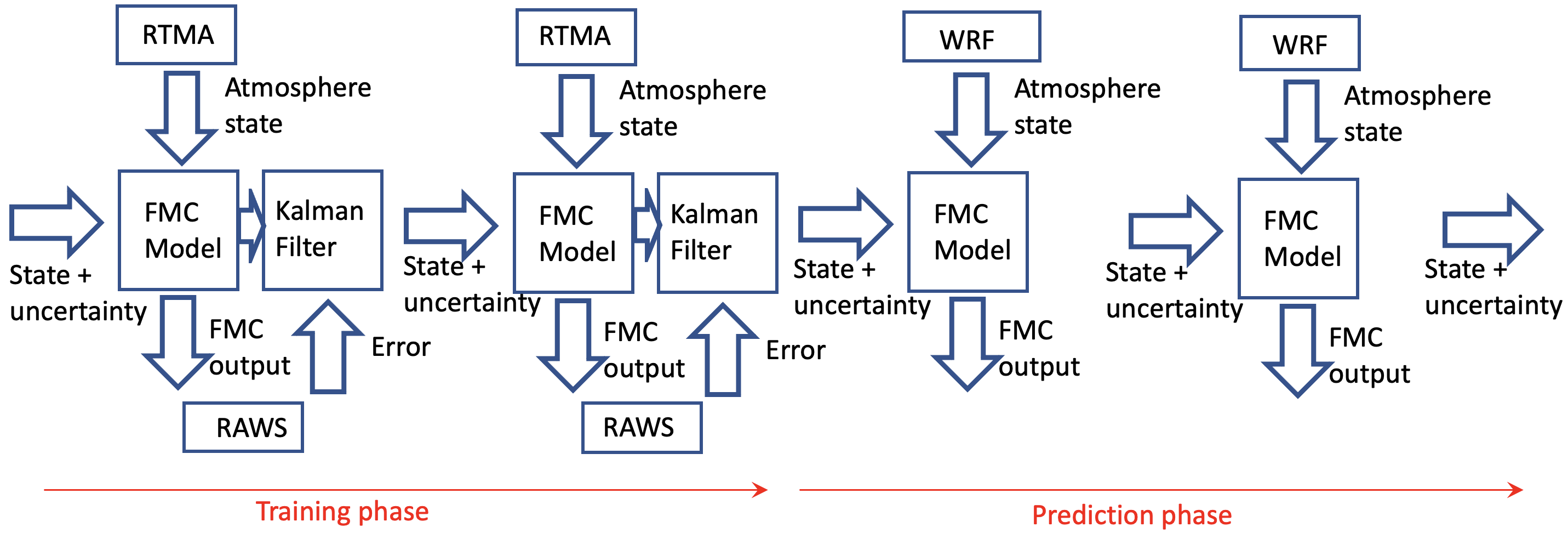
Figure 1: Data flow in the existing model with Kalman filter.

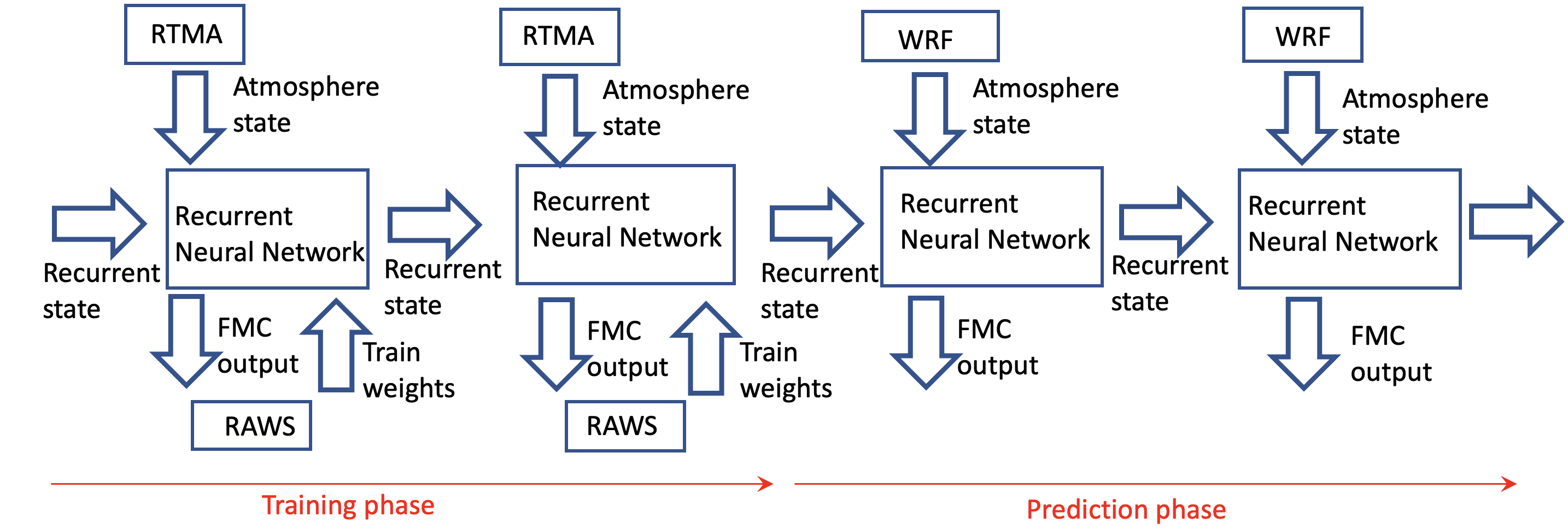
Figure 2: Data flow with the Recurrent Neural Network.

The FMC $m(t)$ in wood is the mass of water as % of the mass of dry wood, and it changes with time $t$ and atmospheric conditions. A simple empirical model of the evolution of $m(t)$ in a wood stick in constant atmospheric conditions is the stick losing water if $m\left(t\right)>E_{d}$, the drying equilibrium, and gaining water if $m\left(t\right)<E_{w}$, the wetting equilbrium, with a characteristic time constant $T$ given by the stick diameter ($T=10$h for 10h fuel). The values of $E_{w}$ and $E_{d}$, $E_{w}<E_{d}$, are computed from atmospheric conditions, namely relative humidity and temperature. We add to both a correction $\Delta E$, assumed constant in time and to be identified from data. This gives a system of differential equation on the interval $\left[t_{k},t_{k+1}\right]$ for the augmented state $u=\left(m,\Delta E\right)$ of dimension 2,

$$\frac{dm}{dt} =\frac{E_{w}+\Delta E-m(t)}{T}\text{\ if }m(t_{k})<E_{w}+\Delta E,\quad\frac{dm}{dt}=\frac{E_{d}+\Delta E-m(t)}{T}\text{\ if }m(t_{k})>E_{d}+\Delta E,\quad$$

$$\frac{dm}{dt} =0\text{ if }E_{w}+\Delta E\leq m(t_{k})\leq E_{d}+\Delta E,\quad\frac{d\Delta E}{dt}=0.$$

We apply the extended Kalman filter to the evolution $u\left(t_{k}\right)\mapsto u\left(t_{k+1}\right)$ with the observations $m\left(t_{k}\right)=d\left(t_{k}\right)$+noise.

The FMC Model and Kalman filter in the data flow in Fig. 1 implement a nonlinear operator. Since the operator is the same at all times $t_{k}$, it is applied recurrently. We seek to identify this operator by a Neural Network (NN) (Fig. 2), which then becomes a RNN.

3 Recurrent Neural Network

Filtering as an application of NNs is now classical. E.g., RNN was trained to match the Kalman filter [1] and synthetizing neural filters [3] estimate both an optimal filter and a model. For contemporary RNN basics, see, e.g., [2, Ch. 15]. Our goal is to build a RNN in the context of current high-performance high-level software, such as Keras, to translate a time series of the atmospheric data in the form of features $E_{d}$, $E_{w}$ to a time series of FMC values $m$.

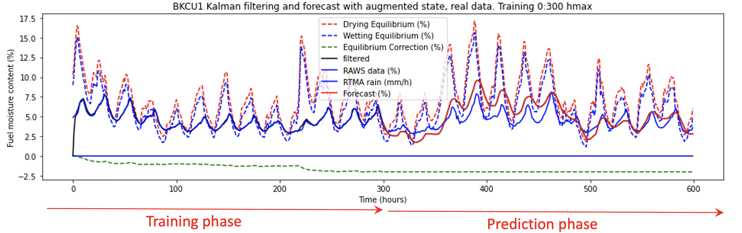
Figure 3: Learning and forecast with the time-lag model and Kalman filter. The equilibrium correction $\Delta E$ stabilizes in the training. Note a large prediction error from 300 to 600 hours.

‘

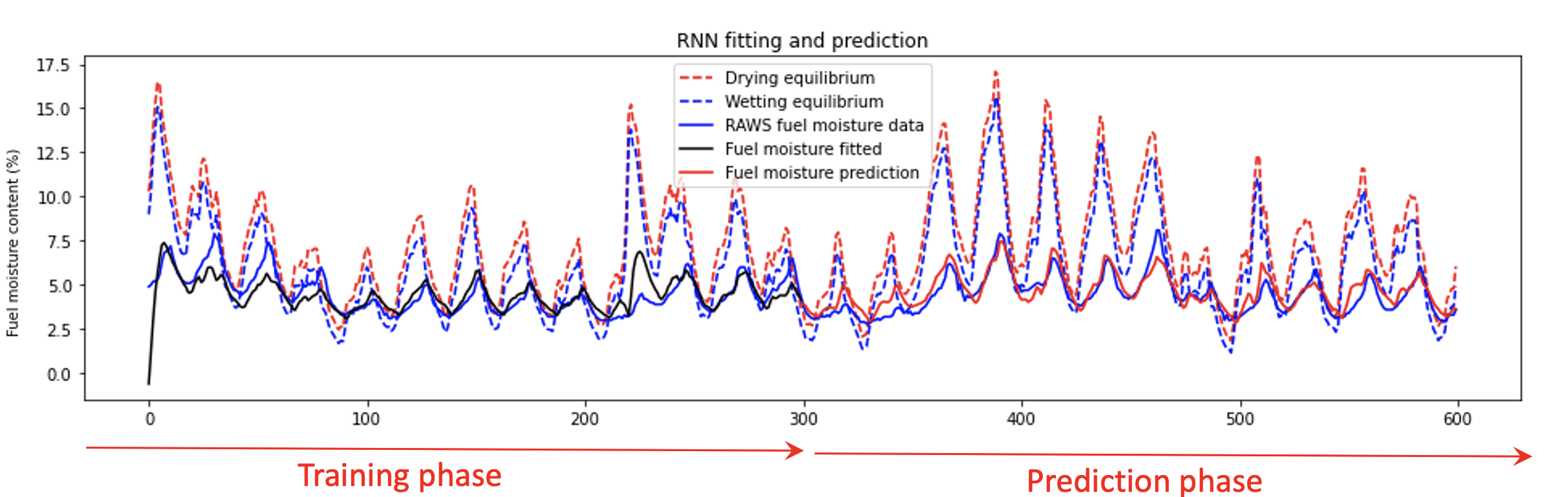
Figure 4: Training and prediction with the Recurrent Neural Network.

Training RNNs is known to be tricky. One reason is that computing the gradient of the loss function by back propagation uses the chain rule applied to the NN operator composed with itself many times, which results in “vanishing” or “exploding” gradients. To overcome this, we train a stateful RNN model [2, p. 532] and limit the number of times the NN operator is composed with itself to a small number of $s$ timesteps. In each batch, the built-in stochastic gradient (SG) optimizer in Keras is presented with a sequence of training samples, each of the form of a short sequence of (input_k+1,…,input_k+s) and (target_k+s), $k=1,2,\ldots$. The inputs are the features $\left(E_{d},E_{w}\right),$ and the targets are the observations from the RAWS FMC sensors. The NN operator is applied to the recurrent state (hidden_k+1,…,hidden_k+s) and the input to produce the new recurrent state (hidden_k+2,…,hidden_k+s+1) and (output_k+s) which is compared with (target_k+s) to compute a contribution to the loss function and its gradient. After the RNN is trained, the optimized weights are copied to an identical stateless NN model [2, p. 534], which is then used for the evaluation of the NN operator in the prediction phase.

Though this procedure is commonly used, it did not work well in this application and the resulting forecast was much worse than when using the extended KF. However, it is straightforward to implement a version of the Euler method for the time-lag differential equation $dm/dt=\left(E-m\right)/T$ by a single neuron with linear activation and a suitable choice of weigths,

$$m_{k+1}=e^{-\Delta t/T}m_{k}+\left(1-e^{-\Delta t/T}\right)E_{k},\qquad\Delta t=t_{k+1}-t_{k}.$$

Here, $m_{k}$ is the hidden state, also copied to the output, and $E_{k}$ is the input. The single neuron RNN worked well on synthetic examples, so we used a hidden layer with linear activation, pre-trained by using the initial weights above.

Our final network had one hidden layer of $6$ neurons pre-trained as above, and two input neurons and one output, all with linear activation. We chose the dimension of the hidden state $6$ to accommodate different time scales. The training used $s=5$ timesteps. The resulting prediction (Fig. 4) was better than from the differential equation model with extended KF (Fig. 3).

4 Conclusion

We have used batch training of a stateful RNN with linear activation and initial weights chosen to make the RNN an exact model in a special case. A hidden layer of several neurons initialized to the same weights then produced a better prediction than a differential equation model with extended KF. Exploiting this principle with more general activations, such as RELU, may enable switching between different behaviours, such as drying, wetting, or rain, or quantification of uncertainty in future.

Acknowledgement: This work was partially supported by NASA grants 80NSSC19K1091, 80NSSC22K1717, and 80NSSC22K1405.

References

- [1] J. P. DeCruyenaere and H. M. Hafez, A comparison between Kalman filters and recurrent neural networks, in [Proceedings 1992] IJCNN International Joint Conference on Neural Networks, vol. 4, IEEE, 1992, pp. 247–251.
- [2] A. Géron, Hands-on machine learning with Scikit-Learn, Keras, and TensorFlow: Concepts, tools, and techniques to build intelligent systems, O’Reilly, 2nd ed., 2019.
- [3] J. T.-H. Lo, Synthetic approach to optimal filtering, IEEE Transactions on Neural Networks, 5 (1994), pp. 803–811.
- [4] J. Mandel, S. Amram, J. D. Beezley, G. Kelman, A. K. Kochanski, V. Y. Kondratenko, B. H. Lynn, B. Regev, and M. Vejmelka, Recent advances and applications of WRF-SFIRE, Natural Hazards and Earth System Science, 14 (2014), pp. 2829–2845.
- [5] J. Mandel, M. Vejmelka, A. K. Kochanski, A. Farguell, J. D. Haley, D. V. Mallia, and K. Hilburn, An interactive data-driven HPC system for forecasting weather, wildland fire, and smoke, in 2019 IEEE/ACM HPC for Urgent Decision Making (UrgentHPC), Supercomputing 2019, Denver, CO, USA, IEEE, 2019, pp. 35–44.
- [6] National Wildfire Coordinating Group, NWCG Standards for Fire Weather Stations, PMS 426-3, March 2019. https://www.nwcg.gov/publications/426-3, retrieved December 2022.
- [7] R. M. Nelson Jr., Prediction of diurnal change in 10-h fuel stick moisture content, Canadian Journal of Forest Research, 30 (2000), pp. 1071–1087.
- [8] D. W. Van der Kamp, R. D. Moore, and I. G. McKendry, A model for simulating the moisture content of standardized fuel sticks of various sizes, Agricultural and Forest Meteorology, 236 (2017), pp. 123–134.
- [9] M. Vejmelka, A. K. Kochanski, and J. Mandel, Data assimilation of dead fuel moisture observations from remote automatic weather stations, International Journal of Wildland Fire, 25 (2016), pp. 558–568.