Evolve Path Tracer: Early Detection of Malicious Addresses in Cryptocurrency

Abstract.

With the boom of cryptocurrency and its concomitant financial risk concerns, detecting fraudulent behaviors and associated malicious addresses has been drawing significant research effort. Most existing studies, however, rely on the full history features or full-fledged address transaction networks, both of which are unavailable in the problem of early malicious address detection and therefore failing them for the task. To detect fraudulent behaviors of malicious addresses in the early stage, we present Evolve Path Tracer which consists of Evolve Path Encoder LSTM, Evolve Path Graph GCN, and Hierarchical Survival Predictor. Specifically, in addition to the general address features, we propose Asset Transfer Paths and corresponding path graphs to characterize early transaction patterns. Furthermore, since transaction patterns change rapidly in the early stage, we propose Evolve Path Encoder LSTM and Evolve Path Graph GCN to encode asset transfer path and path graph under an evolving structure setting. Hierarchical Survival Predictor then predicts addresses’ labels with high scalability and efficiency. We investigate the effectiveness and generalizability of Evolve Path Tracer on three real-world malicious address datasets. Our experimental results demonstrate that Evolve Path Tracer outperforms the state-of-the-art methods. Extensive scalability experiments demonstrate the model’s adaptivity under a dynamic prediction setting.

1. Introduction

The past decade has witnessed the growth of cryptocurrency as decentralized global financial systems. Unfortunately, it has long been criticized for accommodating various cyber-crimes due to its anonymity. According to the recent Crypto Crime Report by Chainalysis, 2022 was the biggest year ever for crypto-crime, with $3.8$ billion dollar worth of crypto asset stolen. Researchers and practitioners have made significant efforts to combat fraudulent activities and identify associated malicious addresses, particularly for Bitcoin (BTC) due to its singularly important leadership remained unshakable among all cryptocurrencies.

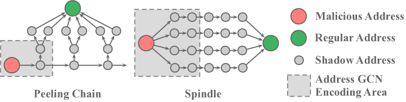
Figure 1. Two asset flow patterns of malicious addresses. Address transaction network methods may suffer shadow address issues as they only consider neighbors within 2 or 3 hops. By encoding asset transfer paths (from red node to green node), the model can capture more comprehensive patterns.

However, there are three major limitations in current methods:

• Ineffective for early detection. Most previous works adopt random walk and graph neural network (Harlev et al., 2018a; Wu et al., 2021; Weber et al., 2019; Chen et al., 2020) to improve the performance of general malice detection. But most of them require a full-fledged address network which is unavailable under the early stage settings, as early transaction graphs are usually unconnected and fast-evolving, and most addresses are unlabelled.

• Type-specific features are not generalizable. Malice are evolving fast. It is impossible to build a unique feature set for every new malicious activity. Most methods (Reid and Harrigan, 2013; Androulaki et al., 2013; Jourdan et al., 2018) are designed for specific malicious behaviors and cannot be generalized to other types and other cryptocurrencies. Although some studies (Nerurkar et al., 2020) can detect categories of entities, the features are too general to describe malicious transaction patterns.

• Challenge of shadow account issues. Most address transaction network methods may suffer the shadow address issues. As shown in Fig. 1, the perpetrators create a bunch of shadow addresses, and the illicit asset will be transferred through the paths constructed by these addresses and eventually converge at a particular destination. Usually, these paths are extremely long compared to the encoding area (2 or 3 hops) of address network methods (Weber et al., 2019), as such address networks cannot encode transaction patterns comprehensively. If expanding the encoding area, they may incur scalability issues and run into the problem of minority class dilution.

Considering the first limitation, in this work, we first set up the Early Malicious Address Detection (EMAD) task, which is urgent but seldom discussed by existing studies. Then we design a novel model Evolve Path Tracer to detect malicious addresses at an early stage. For the second requirement, considering malicious addresses’ objective is to transfer illicit money to a legal place. Even though the behavior patterns differ for various address types, we can still derive their intentions by monitoring their asset transfer patterns. We therefore develop a path extractor to extract those significant Asset Transfer Paths to characterize the early-stage transactions of various malicious addresses effectively.

For the last requirement, illicit activities are usually organized together for specific purposes, and the behavior patterns evolve fast during the early stage. As a result, encoding each path individually may miss critical information. Therefore, after encoding paths independently with path encoder LSTM, we build an asset path GCN module to encode the inter-relation among paths. In this graph, asset transfer paths connect to one other if they share the same intersection addresses. As shown in Fig. 1, by encoding paths with the same destination together, we can discover the hidden intention of malicious addresses and address the tricky problem of shadow addresses challenging most address GCN models. Moreover, static encoding models cannot capture the dynamism of fast-evolving early transfer patterns. This problem is similar to the one indicated by (Pareja et al., 2020), we therefore embed the evolving mechanism into our path encoder LSTM and path GCN module for more sophisticated path representations under the dynamic setting.

Considering the scalability issue in the real-world application, we implement a Hierarchical Survival Prediction module to alleviate the workload of feature preparation during the prediction. Previous prediction results can be directly used in the next time step, which empowers the model with a faster prediction speed and the ability to deal with a dynamic setting. In summary, the contributions of this paper can be summarized as follows:

• The Asset Transfer Paths are proposed for the EMAD task, which is urgent but seldom discussed. These paths exhibit high versatility in monitoring transaction patterns of various malicious behaviors in the early stage. This novel concept can be potentially applied to all current cryptocurrency systems.

• We propose the Evolve Path Tracer model that can fully utilize the asset transfer paths to dynamically encode various transaction patterns with path encoder LSTM. Besides, to relieve the problem of shadow addresses, the model can also encode the paths’ structural relationship under a dynamic setting with a novel evolve path graph GCN module. The versatility and flexibility are unachievable by other existing models.

• We conduct extensive evaluations to assess the model’s effectiveness, and the results show that Evolve Path Tracer deliver a substantially better performance for three different illicit address datasets than the state-of-the-art models. Also, owing to the Hierarchical Survival Prediction module, our Evolve Path Tracer can effectively predict addresses’ labels and scales well for increasing data.

We organize the remaining sections as follows. In Section 2, we classify and review related works. In Section 3, we define the problem of Early Malicious Address Detection. Then we explain the construction of the asset transfer path and path graph in Section Section 4, and introduce the details of Evolve Path Tracer in Section 5. Finally, we present experimental results in Section 6 and conclude this paper in Section 7.

2. Related Work

The methods for malice detection on cryptocurrencies can be classified into three categories, namely case analysis, machine learning, and graph based methods. We review these methods according to their types.

2.1. Case Analysis

Case analysis mainly focuses on addresses’ behaviors in a certain case. Reid et al. (Reid and Harrigan, 2013) identified entities by considering similar transaction times over an extended timeframe. Androulaki et al. (Androulaki et al., 2013) considered several features of transaction behavior, including the transaction time, the index of addresses, and the value of transactions. Jourdan et al. (Jourdan et al., 2018) explored five types of features, including address features, entity features, temporal features, centrality features, and motif features. Vasek et al. (Vasek and Moore, 2015) gave a list of Bitcoin scams and conducted a statistical study. Case-Related features are often helpful in interpreting certain cases based on heuristic clustering and tainted fund flow. However, these methods require intensive case analysis, and most of the insights are only available in some specific cases, let alone apply to other platforms with complex heterogeneous relationships in general (Sun et al., 2012; Kuck et al., 2015).

2.2. Machine Learning

Machine Learning methods can automatically learn general address features to increase model’s generalization ability. Yin et al. (Yin and Vatrapu, 2017) applied supervised learning to classify entities that might involve in cybercriminal activities. Akcora et al. (Akcora et al., 2020) applied the topological data analysis (TDA) approach to generate the bitcoin address graph for ransomware payment address detection. Shao et al. (Shao et al., 2018) embedded the transaction history into a lower-dimensional feature for entity recognition. Nerurkar et al. (Nerurkar et al., 2020) used several general features for classifying different address categories. The general address features improve the model’s generality significantly. However, they are challenging to characterize addresses’ behaviors comprehensively. Particular transaction patterns of asset flow are difficult to be reflected in these characteristics. Besides, some models (Al-rimy et al., 2019; Chen et al., 2019; Roy and Chen, 2021) can detect crypto-malware early, TLR model (Gutflaish et al., 2019) learns the expected likelihood score from training data and uses the disparity between predicted and observed likelihood scores. while they require malware’s operation logs or code corpus, which are unavailable in most cases where we only have on-chain data.

2.3. Graph Based Methods

Graph-based methods focus on the interaction patterns between object addresses and related addresses. Harlev et al. (Harlev et al., 2018a) considered transaction graph features to predict entity types. Wu et al.(Wu et al., 2021) proposed two types of network motifs to detect BTC mixing service addresses. Weber et al. (Weber et al., 2019) encodes address transaction graph with GCN, Skip-GCN, and Evolve-GCN to detect illicit addresses. Chen et al.(Chen et al., 2020) proposed E-GCN for phishing node detection on the ETH platform. Tam et al.(Tam et al., 2019) proposed EdgeProp to learn the large-scale transaction network representations for illicit account identification. Lin et al.(Lin et al., 2020) proposed random walk-based embedding methods to encode specific network features for node classification. By changing the sampling strategy, Wu et al.(Wu et al., 2020) proposed the Trans2Vec model for a similar task. Li et al.(Li et al., 2022) encoded the temporal information of historical transactions for phishing detection. Chen et al.(Chen and Tsourakakis, 2022) proposed the AntiBenford subgraph framework for anomaly detection in the Ethereum. Network-based methods perform well for retrospect analysis, as they encode the structural information. Besides, most graph-based anomaly detection can also be potentially implemented. AMNet (Chai et al., 2022) and BWGNN (Tang et al., 2022) aim to discriminate anomaly nodes with the spectral energy distribution difference. However, in the early stages, the performance degrades greatly if the networks are of sparse structures for the emerging networks with few connections(Zhang et al., 2017). Also, due to the limitation of scalability, these methods suffer shadow address issues as mentioned in Fig. 1. Expanding the encoding area may lead to Over-Smoothing issues and the dilution of the minority class (Liu et al., 2021) under the data-unbalanced setting (Zhang et al., 2022; Jiang et al., 2022; Zhao et al., 2022).

Among all cryptocurrencies, Bitcoin (BTC) has the largest volume, and is considered as the prototype for other cryptocurrency platforms (e.g., ETH, EOS with smart contracts), most BTC-based methods are thus compatible with other cryptocurrency platforms. Following previous practitioners, we also focus on detecting malicious addresses on BTC.

3. Problem Definition

For each BTC transaction ($TX$), we analyze its input TX set $I$= $\{i_{1},i_{2},\dots,i_{|I|}\}$ and an output TX set $J$= $\{j_{1},j_{2},\dots,j_{|J|}\}$. Each $tx$ records token distribution between $I$ and $J$. Narratively speaking, the incoming tokens flow into a pool and then flow to the outgoing transactions according to the prior agreement proportion . There is no record of how many tokens flow from an Input $i$ to an Output $j$. We thus have to build a complete transaction bipartite graph for this $TX$ and generate $|I|\times|J|$ transaction pairs in total. In other words, a transaction has $|I|\times|J|$ transaction pairs inside. If an address acts as the input address of $TX$, we denote $TX$ as the address’s $Spend$ transaction. Otherwise, $Receive$ transaction.

By the $t_{m}$-th time step, $D_{t_{m}}$=$\{d^{i}_{t_{m}}\}_{i=1}^{N}$=$\{(l^{i},T_{in,t_{m}}^{i},T_{out,t_{m}}^{i})\}_{i=1}^{N}$ is the input data, where $l^{i}\in\{0,1\}$ is the label of Address $i$, and $0$ or $1$ stands for regular and malicious addresses respectively. $T_{in,t_{m}}^{i}$=$[TX_{in,1}^{i},\dots,TX_{in,N_{in,t_{m}}}^{i}]$ are the $Spend$ transaction sets and $T_{out,t_{m}}^{i}$=$[TX_{out,1}^{i},\dots,TX_{out,N_{out,t_{m}}}^{i}]$ are the $Receive$ transaction sets of Address $i$ by the $t_{m}$-th time step respectively.

Early Malicious Address Detection (EMAD). Given a set of addresses $A$, and $D_{t_{m}}$ at timestep $t_{m}$, the problem is to build a binary classifier $F$ such that

(1) $$F(d^{i}_{t_{m}})=\begin{cases}1&\text{if Address $i$ is malicious}\\ 0&\text{Otherwise}\end{cases}.$$

In the early detection task, to prevent the model predicts conflict labels at different timesteps, which will confuse users, we thus require the prediction to be consistent and predict the correct label as early as possible. We denote the confident time as $t_{c}$, where all classifier predictions $F$ after $t_{c}$ are consistent. The smallest $t_{c}$ is denoted as $t_{f.c}$. Our purpose is to train a classifier that predicts the correct label of an address with a smaller $t_{f.c}$.

4. Asset Transfer Path and Path Graph

As we know the destination and the source of asset transfer can provide critical information, we thus propose the Asset Transfer Paths and Asset Transfer Path Graph to reflect: 1) the characteristics of each path, 2) the interaction between paths, and 3) the characteristics of the asset source (destination).

Take Address $i$’s $Recieve$ transaction set as an example. For a $Receive$ transaction in the set, suppose we find its significant asset source, which is also a transaction, then we link them to form an asset transfer pair. After we trace the asset source iteratively, the asset transfer pairs form an asset transfer path naturally. If all paths come from the same source, then we can say that, at a particular time, there are multiple transactions initiated at the same time, and all these transactions’ destinations are Address $i$. If we encode each path as a node, these nodes can be connected through this source of funds, thus forming a graph.

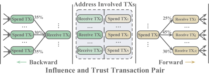
Figure 2. Asset transfer pairs. Given an address, we collect its transaction history (All its Receive and Spend TXs in the dotted box). For each Receive TX, we trace its asset source from the inflow (Green Spend TXs) to build Influence TX pairs. For each Spend TX, we trace its asset destination from the outflow (Yellow Receive TXs) to build Trust TX pairs. $N=N_{in,t_{m}}$, $M=N_{out,t_{m}}$.

4.1. Transaction Pair and Path Construction

Not all transaction pairs help identify illicit addresses. Those noteworthy pairs typically constitute a significant amount portion of the entire transaction. As illustrated in Fig. 2, $TX_{j}$ receives assets from three spend TXs (each contributing $35\%$, $30\%$, and $35\%$ to the total transaction amount). On the other hand, the spend $TX_{i}$ transfers out BTCs to three receive TXs (with a distribution of $25\%$, $45\%$, and $30\%$ as in this example). Given an Address $i$ and a time step $t_{m}$, TXs in the shaded dotted-lined box represent all spend TXs, and receive TXs occurred up to timestep $t_{m}$ associated with Address $i$.

As mentioned in Section 3, given a set $I$= $\{i_{1},i_{2},\dots i_{|I|}\}$ of $|I|$ spend transactions to an receive transaction $j$ and the set $\{{I\rightarrow j}\}$ of all transaction pairs, i.e., $\{{I\rightarrow j}\}$=$\{(i_{1},j),(i_{2},j),\ldots,(i_{|I|},j)\}$, we define Influence Transaction Pair as follows: Given an influence activation threshold $\theta$, $(i_{k},j)$ is called an Influence Transaction Pair for transaction $j$, if the amount of transaction pair $(i_{k},j)$ ($1\leq k\leq|I|$) contributes at least a certain proportion of the received amount of transaction $j$, i.e, $\hat{A}(i_{k},j)\geq\theta\times\hat{A}(\{{I\rightarrow j}\})$ where $\hat{A}(\cdot)$ denotes the amount of a transaction pair or the sum of all transaction pairs.

Similarly, given a set $J$= $\{j_{1},j_{2},\dots j_{|J|}\}$ of $|J|$ transactions, and a transaction $i$, and the set $\{{i\rightarrow J}\}$ of all transaction pairs whose spend transaction is $i$, i.e., $\{{i\rightarrow J}\}$=$\{(i,j_{1}),(i,j_{2}),\ldots,(i,j_{|J|})\}$. If there exists a receive transaction $j_{k}$ ($1\leq k\leq|J|$), such that transaction $i$ transfers at least a certain proportion of its spend amount to it, this transaction pair is called a Trust Transaction Pair for transaction $i$, as it indicates a certain form of trust from $i$ to $j_{k}$ in terms of asset transfer.

To construct asset transfer paths, given an influence transaction pair $(i_{k},j)$, we can conclude that transaction $j$ obtains at least a significant amount (based on the threshold) of the asset in this transaction from transaction $i_{k}$. Accordingly, given a transaction $j$, if there exists a sequence of transaction pairs such that (I) each pair is an influence transaction pair; (II) the spend transaction of each pair is the receive transaction of the previous pair; and (III) the receive TX of the last pair is transaction $j$, we call such a sequence an Backward Path for $j$ as indicated by the green arrow in Fig. 2. It reveals where $j$ obtains the asset and can be used to trace back to the source of the asset. The detail to prepare the backward asset transfer path is shown in Algorithm 1. Similarly, we can define a Forward Path to trace the destinations of transaction $i$’s asset flow. For brevity, we would refer to both the Backward Path and Forward Path as Asset Transfer Paths.

As shown in Fig. 3, for Receive Tx R-1 in the Flow of Receive Tx, after we trace its asset source, we can get three critical transfer pairs, namely (10 $\rightarrow$R-1, 11 $\rightarrow$R-1, 12 $\rightarrow$R-1). As shown in Backward Asset Transfer Path, iteratively, we can get four paths (P-1, P-2, P-3, P-5) ended with R-1.

4.2. Asset Transfer Path Graph

The address transaction graph methods may suffer from the perturbation of shadow addresses and the scalability issues caused by mixing services. However, even though malicious addresses use mixing services, their suspicious asset transfer paths will still converge. Therefore, unlike the previous address-based graph, we build graphs based on the asset transfer path. As shown in Fig. 3, in the path graph part, each node represents an asset-transfer path. If two paths share the same source (for backward paths) or destination (for forward paths), we then connect them with an edge, and we thus can get a group of fully-connected graphs. Here we also take Backward Asset Transfer Paths as examples. Among them, three paths(P-1, P-2, P-3) have the same source (Tx-1 colored green). Also, another path (P-4) ended with R-2 is also initiated by the same source, we thus group them into a path graph, which is colored green, as shown in the Backward Path Graph.

Since every source or destination has a binding address at a specific timestep, we use the feature of this binding address at this time point to represent the edge feature in the corresponding graph. The Address Features (AF) and transaction features are elaborated in Appendix.

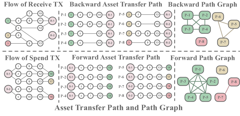
Figure 3. Asset transfer path and path graph. By tracing the asset source iteratively, we get a series of Influence TX pairs. We combine them end-to-end to form Backward Asset Transfer Path (Similar to Forward Asset Transfer Path). If paths have the same source or destination, we connect them through their intersection to form a path graph (Graph in the same color). Different colors stand for different starting or ending points.

5. Evolve Path Tracer

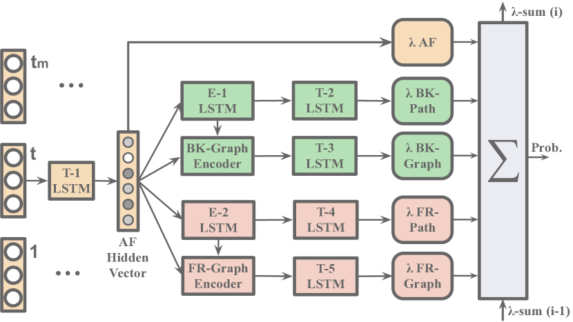
Figure 4. Detailed pipeline of Evolve Path Tracer. At each timestep, five Temporal-LSTM models (T LSTM) encode temporal information of different features. The Evolve Path Encoder LSTM (E LSTM) and Evolve Path Graph GCN (Graph Encoder) will be updated to encode asset transfer paths and path graphs dynamically. For module detail description, please refer to Table LABEL:tab:module_explain.

As shown in Fig. 4, at the $t$ th timestep, five Temporal-LSTM models (T-1 to T-5 LSTM) are implemented to encode temporal information of the following input data: 1: Address Feature (AF), 2: Backward Path (BK-Path), 3: Backward Graph (BK-Graph), 4: Forward Path (FR-Path), 5: Forward Graph (FR-Graph).

Take the backward branch as an example (green branch), we input the current AF to update T-1 LSTM. However, as we have multiple backward paths at each timestep, to update other LSTMs, we need to encode each path and aggregate them as the inputs for these LSTMs. Therefore, we implement E-1 LSTM (Backward Evolve Path Encoder LSTM) to encode each backward path into a path vector. Meanwhile, to reflect the path structure’s dynamism, the parameters of E-1 LSTM are calculated based on the current ($t$ th) hidden vector of T-1 LSTM and the previous ($t-1$ th) hidden vector of T-2 LSTM. With an attention-weighted summation, all these backward path vectors are aggregated as the input to update T-2 LSTM. Besides, BK-Graph Encoder (Backward Evolve Path Graph GCN) incorporates path-graph structure in these backward path vectors. Then, following similar processings, these structure-aware path vectors are aggregated as the input to update T-3 LSTM. The forward branch follows the same mechanism to update T-4 and T-5 LSTMs. Concretely, at the $t$ th timestep, the process can be summarized in five steps:

• Step-1. To encode the temporal information of the Address Feature(AF), we input current ($t$ th timestep) AF into T-1 LSTM to get the T-1 hidden vector.

• Step-2. We concatenate the T-1 hidden vector with the previous ($t-1$ th timestep) T-2 and T-3 hidden vectors to generate parameters for E-1 LSTM and BK-Graph Encoder.

• Step-3. E-1 LSTM encodes each path into a corresponding path vector. Then we weighted sum these path vectors to update T-2 LSTM.

• Step-4. BK-Graph Encoder updates path vectors with graph information. Similarly, we weighted sum these vectors to update T-3 LSTM.

• Step-5. After similar processing for the forward branch, we use the hidden vectors of five temporal LSTM (T-1 to T-5) to predict the current label of the address.

5.1. Evolve Path Encoder LSTM

The Address Feature is the basis for modeling the address transaction pattern. We implement an LSTM (T-1 LSTM) to encode Address Feature’s temporal information and guide the processing in other modules.

(2) $$h_{t}^{T_{1}},c_{t}^{T_{1}}=\mbox{LSTM}^{T_{1}}(f^{u}_{t},h_{t-1}^{T_{1}},c_{t-1}^{T_{1}}),\\$$

where $h_{t}^{T_{1}}\in\mathbb{R}^{d}$ and $c_{t}^{T_{1}}\in\mathbb{R}^{d}$ are the hidden state and the cell state of T-1 LSTM at time $t$. $f^{u}_{t}\in\mathbb{R}^{d_{n}}$ is the address feature at time $t$. $d$ and $d_{n}$ are the dimensions of the hidden state and address feature.

As mentioned in Section 4, the asset transfer path is composed of a series of transaction nodes. The lengths of these paths are different. To encode them uniformly, we project an original path $P_{ori}$ to a uniform path $P_{u}$ with the length of $L_{u}$. Given an original path $P_{ori}$ with length of $L_{ori}$, the zoom ratio is calculated by $R_{z}$ = $L_{ori}/L_{u}$, then the $i$-th (start from $0$) node in $P_{u}$ is calculated by the average feature of the ($\lfloor i\times{R_{z}}\rfloor$)-th node to the ($\lceil(i+1)\times{R_{z}}\rceil$-1)-th node of $P_{ori}$, where $\lfloor\cdot\rfloor$ and $\lceil\cdot\rceil$ are round down and round up functions. Then, we denote the uniform path as:

(3) $$\mathit{P_{u}}=[p_{1},p_{2},\dots,p_{L_{u}}],$$

Path structures are different on different addresses and timesteps. We may lose dynamic information with a static encoder. In Evolve-GCN (Pareja et al., 2020), the weights are updated by previous weights or those representative nodes but may dismiss the individual address property. Instead, to update the parameters of a specific Path Encoder LSTM module, we generate the new weights with the concatenation of $h_{t}^{T_{1}}$ and previous hidden state of corresponding Temporal LSTM. For the $j$-th node in the input asset transfer path, backward Evolve Path Encoder LSTM (E-1 LSTM) computes the following function:

(4) $$h^{E_{1}}_{j},c^{E_{1}}_{j}=\mbox{LSTM}^{E_{1}}([h_{t}^{T_{1}}||h_{t-1}^{T_{2}}],{h_{j-1}^{E_{1}}},{c_{j-1}^{E_{1}}}),$$

where $||$ stands for concatenation, $h_{t-1}^{T_{2}}\in\mathbb{R}^{d}$ is the hidden state of T-2 LSTM at timestep $t$-$1$. T-2 LSTM encodes the temporal information of the backward asset transfer path set. Besides, all parameters in the E-1 LSTM are represented by the multiplication of $[h_{t}^{T_{1}}||h_{t-1}^{T_{2}}]$ and corresponding learnable weights. Finally, each backward asset transfer path is denoted as the final hidden state $h^{E_{1}}_{L_{u}}$ of E-1 LSTM. The representation of the $i$-th path at timestep $t$ is $f^{p}_{i,t}$.

For path aggregation, we expect to select more informative paths, we thus adopt multi-head attention for the selection.

(5) $$a_{i,t}^{j}=W^{a,j}\mbox{tanh}(W^{p,u}[f^{p}_{i,t}||h_{t}^{T_{1}}]);\quad{\alpha}_{i,t}^{j}=\mbox{Softmax}(a_{i,t}^{j}),$$

(6) $$\hat{f}^{p}_{t}=||_{j=1}^{{M}^{p}}\hat{f}^{p,j};\quad\hat{f}^{p,j}_{t}=\sum_{i=1}^{N_{E_{1}}}{\alpha}_{i,t}^{j}f^{p}_{i,t},$$

where $f^{p}_{i,t}$ is the representation of the $i$-th path at timestep $t$. $W^{p,u}\in\mathbb{R}^{\frac{d}{M^{p}}}\times{2d}$ and $W^{a,j}\in\mathbb{R}^{{1}\times{\frac{d}{M^{p}}}}$ are learnable matrices, $j$ stand for the index of the attention head, $M^{p}$ is the total head number. $N_{E_{1}}$ is the backward asset transfer path number. where $\hat{f}^{p,j}_{t}$ is the weighted summed path feature vector of $j$-th head, $\hat{f}^{p}_{t}$ is the concatenation of all heads’ output. The hidden state $h_{t}^{T_{2}}$ and cell state $c_{t}^{T_{2}}$ of T-2 LSTM are updated as:

(7) $$h_{t}^{T_{2}},c_{t}^{T_{2}}=\mbox{LSTM}^{T_{2}}(\hat{f}^{p}_{t},h_{t-1}^{T_{2}},c_{t-1}^{T_{2}}).$$

5.2. Evolve Path Graph GCN

If several paths are initiated by or converge at the same transaction, it may indicate certain suspicious patterns. By encoding the relationships between these paths, the model can capture critical transaction patterns. Also, due to the volatility of the path graph, we may lose the discriminative characteristics with a static model. To resolve this challenge, we propose Evolve Path Graph GCN. Take backward asset transfer paths as an example, the nodes in the path graph are updated as follows:

(8) $$H_{t}^{g} =[h_{t}^{T_{1}}||h_{t-1}^{T_{3}}],$$

$$f^{g}_{t} =\sigma(\mathcal{\tilde{D}}^{-\frac{1}{2}}\mathcal{\tilde{A}}\mathcal{\tilde{D}}^{-\frac{1}{2}}(f^{p}_{t}W^{g}H_{t}^{g})),$$

$$\tilde{\mathcal{A}} =\mathcal{A}+\mathcal{I};\quad\mathcal{A}_{i,:,j}=(W^{e}H_{t}^{g})S_{i,j},$$

$$\mathcal{\tilde{D}} =\mbox{diag}(\sum_{j}(A_{i,j}+\mathcal{I}_{i,j})),$$

where $h_{t-1}^{T_{3}}\in\mathbb{R}^{d}$ is the hidden state of T-3 LSTM at time $t$-$1$. T-3 LSTM encodes the temporal information of the backward path graph. $f^{p}_{t}\in\mathbb{R}^{{N_{E_{1}}\times{d}}}$ are the representations of path set at timestep $t$. $A\in\mathbb{R}^{{N_{E_{1}}}\times{d}\times{N_{E_{1}}}}$ and $\mathcal{I}\in\mathbb{R}^{{N_{E_{1}}}\times{d}\times{N_{E_{1}}}}$ are the adjacent matrix and the identity matrix respectively. If the $i$-th path and $j$-th path have the same source, then $A_{i,:,j}$=$\mathbf{1}\in\mathbb{R}^{d}$. Otherwise, $A_{i,:,j}$=$\mathbf{0}\in\mathbb{R}^{d}$. If the $i$-th path and $j$-th path have the same source, $S_{i,j}\in\mathbb{R}^{d_{n}}$ is the intersection address feature of path $i$ and path $j$. Otherwise, $S_{i,j}$=$\mathbf{0}\in\mathbb{R}^{d_{n}}$. $W^{g}\in\mathbb{R}^{{d}\times{d}\times{2d}}$ and $W^{e}\in\mathbb{R}^{{d}\times{d_{n}}\times{2d}}$ are learnable weights, and they project $H_{t}^{g}$ to the weights of the corresponding projection layers. So $\mathcal{A}\in\mathbb{R}^{{N_{E_{1}}}\times{d}\times{N_{E_{1}}}}$.

We denote the output of Evolve Path Graph GCN encode as interaction-aware path vectors. Resemble the previous calculation, we adopt multi-head attention to select significant signals from these interaction-aware path vectors. We denote the $\hat{f}^{g}_{t}$ as the final result of multi-head attention of interaction-aware path vectors. The hidden state $h_{t}^{T_{3}}$ and cell state $c_{t}^{T_{3}}$ of T-3 LSTM are updated as:

(9) $$h_{t}^{T_{3}},c_{t}^{T_{3}}=\mbox{LSTM}^{T_{3}}(\hat{f}^{g}_{t},h_{t-1}^{T_{3}},c_{t-1}^{T_{3}}).$$

5.3. Hierarchical Survival Predictor

Due to the property of consistent prediction, survival analysis (Zheng et al., 2019) is proved to be effective in the early detection task. The survival function $S(t)$ of an event represents the probability that this event has not occurred by time $t$. The hazard rate function $\lambda_{t}$ is the event’s instantaneous occurrence rate at time $t$ given that the event does not occur before time $t$. In our case, the observation time is discrete in our case, we use $t$ to denote a timestamp. The association between $S(t)$ and $\lambda_{t}$ can be calculated as:

(10) $$S(t) =P(T\geq{t})=\sum_{k=t}^{\infty}f(x),$$

$$\lambda_{t} =f(t)/S(t);\quad S(t)=\mbox{exp}({-\sum_{k=1}^{t}\lambda_{k}}).$$

Considering the model’s scalability during the real-time prediction, we define the event as “the address is benevolent” and we call hazard rate as benevolent rate. As the majority addresses are negative (benevolent), if the address is classified as benevolent, we remove it from the monitoring list to reduce the computation cost.

To get more consistent predictions, previous work (Zheng et al., 2019) deployed a Softplus function ${\lambda}_{t}({x_{t}})=ln(1+\mbox{exp}({x_{t}}))$ to guarantee the hazard rate ${\lambda}_{t}$ is always positive. Hence, the survival probability $S(t)$ monotonically decreases. However, the model can hardly classify addresses correctly in the early hours. Some false predictions will never be corrected with the monotonically decreasing survival probability. Therefore, we release this restriction with a $tanh$ activation function for benevolent rate calculation. The consistency is assured by Consistency Loss Function which will be discussed later.

We designed five parallel benevolent rates corresponding to each kind of information (address feature, path feature (backward and forward), and graph feature (backward and forward)). At time step $t$, the calculation of these benevolent rates and the prediction are as follows:

(11) $$\lambda_{j,t} =\mbox{tanh}({W^{hz}_{T_{j}}h_{t}^{T_{j}}}),$$

$$\hat{y}^{t} =\mbox{exp}(-\mbox{ReLU}(\sum_{i=1}^{t}\sum_{j=1}^{5}\lambda_{j,i})),$$

where $W^{hz}_{T_{j}}\in\mathbb{R}^{1\times{d}}$ is the linear projection matrices for the output of T-j LSTM. At each time step, survival analysis first sums all previous benevolent rates, then it sums the current $5$ benevolent rates hierarchically. Once addresses’ current benevolent rates reach a certain threshold, we can remove them from the monitoring list to speed up the prediction and relieve the computing cost in the following hours.

5.4. Training and Dynamical Prediction

Model Training. The model should give higher $S(t)$ to malicious addresses and lower $S(t)$ to benevolent addresses in every time split. For Address $i$, at timestep $t_{m}$, the early detection likelihood function and the negative logarithm prediction $loss^{P}$ are shown as below:

(12) $$likelihood =(1-S(t_{m}))^{1-l_{i}}S(t_{m})^{l_{i}}$$

$$=(1-\mbox{exp}(-\sum_{t=1}^{t_{m}}\sum_{j=1}^{5}\lambda_{j,t}))^{1-l_{i}}(\mbox{exp}(-\sum_{t=1}^{t_{m}}\sum_{j=1}^{5}\lambda_{j,t}))^{l_{i}},$$

$$loss^{P}_{i,t_{m}} ={l_{i}}\sum_{t=1}^{t_{m}}\sum_{j=1}^{5}\lambda_{j,t}+{(l_{i}-1)}ln(1-\mbox{exp}(-\sum_{t=1}^{t_{m}}\sum_{j=1}^{5}\lambda_{j,t})).$$

Besides, $loss^{P}$ is weighted by $\sqrt{t_{m}}$ to avoid the perturbation in the early period due to the data insufficiency.

Consistency-boosted Loss Function. Since the rate function is not guaranteed to be positive in our model, a consistency loss $loss^{C}$ is necessary for consistent predictions. In every time split, the benevolent rate should have the same sign as the previous time split.

(13) $$loss^{C}_{i,t_{m}}=\begin{cases}0&\mbox{sign}(\lambda_{t_{m}-1}*\lambda_{t_{m}})>=0\\ 1&\mbox{else}\end{cases},$$

where $\lambda_{t_{0}}=0$. Similarly, the model should be able to rectify the poor prediction in the early period, the $loss^{C}$ is thus also weighted by $\sqrt{t_{m}}$. The overall loss function is then defined as:

(14) $$\mathscr{L}=\sum_{t=1}^{t_{M}}\sum_{i=1}^{N}\sqrt{t}(loss^{P}_{i,t}+\gamma{loss^{C}_{i,t}}),$$

where N is the dataset size, $\gamma$ is a coefficient to control the contribution between $loss^{P}$ and $loss^{C}$.

Dynamical Prediction. Besides the “Early Stop” mechanism provided by Hierarchical Survival Predictor, our dynamical construction scheme of asset transfer paths can also relieve the time cost of feature preparation. As shown in Fig. 5, the path data can be reused if no new transaction occurs in this interval. If an address has new Receive or Spend transactions, the model will create new backward or forward asset transfer paths accordingly. Moreover, the model also checks the endpoint of the forward paths to determine whether they need to be extended or not.

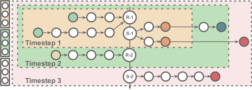
Figure 5. Dynamical Construction of asset transfer path. The three vectors on the left are Address Features corresponding to Timestamp $1$ to Timestamp $3$. Different dash boxes represent input information at different timestamps.

6. Experiment and Analysis

In this section, we perform empirical evaluation to answer the following research questions:

• RQ1: What is the performance with respect to different uniform path lengths?

• RQ2: Does Evolve Path Tracer outperform the state-of-the-art methods for early malicious address detection?

• RQ3: How does each component benefit the final detection performance?

• RQ4: Does the time overhead of data preparation and the model’s scalability satisfy the real-time requirement?

6.1. Data Collection and Preparation

The transaction data are publicly accessible by running a Bitcoin client. We obtained all the data from the $1$-st to the $700,000$-th block for higher credibility, as we only collect addresses verified by enough participants. For a given address, we get the related transaction history based on the APIs exposed by BlockSci (Kalodner et al., 2020). Based on this transaction history, we can calculate the related features and prepare the asset transfer paths and path graphs. More detail about the label acquisition and the statistical properties of the asset transfer path can be found in Appendix A. Table. 1 shows the summarized descriptions: The definition and numbers of positive (Posi), negative (Nega), and Positive/Negative ratio (P/N) for each malicious type (H: Hack, R: Ransomware, D: Darknet).

Table 1. Dataset Statistics

Type	Definition	Posi.	Nega.	P/N(%)
H	Hack and steal tokens	302	6582	4.03
R	Encrypt data for ransoms	3224	21100	15.28
D	Illegal BTC darknets	5838	109937	5.31

6.2. Settings and Metrics

As our purpose is to detect malicious addresses as early as possible, the model should detect them before the institution’s daily settlement when the institutions may find the malice by themselves. Therefore, our experiments focus on early illicit detection during the first day. Although the experiments investigate the performance during the first day, our Evolve path Tracer can work with an arbitrary timespan. To evaluate the performance of our model, we get $24$ hours data with $1$ hour interval, and we average the evaluation metrics on all timesteps. The property evolution and experiment environment can be found in Appendix A.

The selected metrics are accuracy (Acc.), precision (Prec.), and recall (Rec.). Besides, the model should predict correct labels fast to prevent economic loss earlier. Also, due to data insufficiency, the model may predict conflict labels at different timesteps, thus confusing users. Therefore, we require the predictions to be consistent. Similar to earliness and consistency requirements in (Song et al., 2019), we also design the early-weighted F1 score $F1^{E}$ and consistency-weighted score $F1^{C}$ as follows:

(15) $$\mathit{F1^{E}} =\frac{\sum_{i=1}^{N}{F1_{i}/\sqrt{i}}}{\sum_{i=1}^{N}{1/\sqrt{i}}},$$

$$\mathit{F1^{C}} =\frac{\sum_{i=1}^{N-1}{{\sqrt{i}}\times{F1_{i}}\times{\mathbbm{1}_{y_{c}}(y_{i})}}}{\sum_{i=1}^{N-1}{{\sqrt{i}}}},$$

where $i$ is the timestep, $y_{c}$ is the set of predictions where $sign((y_{i}-0.5)\times(y_{i+1}-0.5))>0$. The indicator function $\mathbbm{1}_{y_{c}}(y_{i})=1$ when $y_{i}\in y_{c}$. $F1_{i}$ is the $F1$ score of the prediction at timestep $i$.

6.3. Effects of Uniform Path Length (RQ1)

We further analyze the effects of uniform path length with a simplified AF/Path model (using Address features and Asset Transfer Path features). We test 6 different path lengths on all three datasets (From $2$ to $12$ by the interval of $2$), as shown in Figure 6.

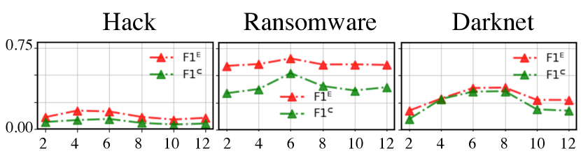
Figure 6. $F1^{E}$ and $F1^{C}$ of different uniform path lengths on three datasets.

A longer uniform path can preserve more information that contributes to better performance. So the model performs better as $L_{u}$ increases at the beginning. However, if the $L_{u}$ is longer than most asset transfer paths, the uniform path may introduce more redundant noise.

Since hack addresses get funds directly from the victim’s account and need to transfer money as soon as possible, its asset transfer path is shorter. As shown in Fig 6, the model achieves the best $F1^{E}$ and $F1^{C}$ scores when setting $L_{u}$ to 4 and 6, respectively. Considering both scores, the model performs best when $L_{u}$ equals $6$. For Ransomware, the ransom demand comes with a deadline. Victims buy bitcoins from exchanges and transfer to criminals, thus slightly increasing the lengths of the asset transfer paths. As shown in Fig. 6, the model performs best When the $L_{u}$ is $6$. For darknet, users could buy and sell illicit goods anonymously via them. Since platforms need to wait for the actions of buyers and sellers, there will be a longer asset transfer path. The model performs best When the $L_{u}$ is between $6$ to $8$. Considering the model’s scalability, in the actual experiment, we also set $L_{u}$ to $6$.

Table 2. Scores of different prediction model. Evo-PT and Evo-PT (E) are our Evolve Path Tracer with/wo “Early Stop” mechanism. Underline stands for best score in the group, Bold stands for best score in all groups.

Type	Model Name	Hack					Ransomware					Darknet
		$Acc.$	$Prec.$	$Rec.$	$F1^{E}$	$F1^{C}$	$Acc.$	$Prec.$	$Rec.$	$F1^{E}$	$F1^{C}$	$Acc.$	$Prec.$	$Rec.$	$F1^{E}$	$F1^{C}$
Machine Learning	DT	0.995	0.347	0.137	0.197	0.197	0.955	0.736	0.432	0.545	0.545	0.982	0.448	0.152	0.227	0.227
	RF	0.996	0.405	0.242	0.303	0.303	0.955	0.735	0.436	0.547	0.547	0.983	0.519	0.109	0.181	0.181
	XGB	0.997	0.347	0.137	0.197	0.197	0.960	0.865	0.435	0.579	0.579	0.985	0.790	0.191	0.308	0.308
Sequen. Deep Learning	GRU	0.928	0.298	0.438	0.354	0.354	0.885	0.558	0.949	0.703	0.703	0.942	0.470	0.838	0.603	0.603
	M-LSTM	0.949	0.418	0.272	0.328	0.333	0.887	0.561	0.969	0.711	0.710	0.951	0.520	0.845	0.642	0.645
	CED	0.909	0.265	0.563	0.360	0.360	0.909	0.617	0.960	0.752	0.751	0.943	0.478	0.829	0.606	0.606
	SAFE	0.918	0.285	0.438	0.271	0.330	0.909	0.616	0.963	0.752	0.752	0.949	0.508	0.838	0.632	0.632
	TMIF	0.913	0.277	0.560	0.356	0.364	0.897	0.623	0.967	0.755	0.761	0.948	0.520	0.840	0.638	0.639
Addr. Graph	GCN	0.920	0.433	0.670	0.501	0.507	0.887	0.564	0.936	0.700	0.706	0.942	0.459	0.613	0.525	0.524
	Skip-GCN	0.917	0.410	0.690	0.443	0.432	0.903	0.603	0.935	0.729	0.735	0.941	0.459	0.629	0.531	0.530
	Evo-GCN	0.893	0.428	0.749	0.427	0.442	0.906	0.613	0.944	0.736	0.746	0.941	0.459	0.633	0.530	0.533
TX. Graph	Evo-PT	0.963	0.607	0.739	0.664	0.668	0.938	0.743	0.869	0.799	0.802	0.963	0.624	0.764	0.686	0.686
	Evo-PT (E)	0.969	0.650	0.731	0.689	0.683	0.940	0.751	0.869	0.802	0.807	0.964	0.625	0.754	0.686	0.687

6.4. Performance Comparison (RQ2)

Table 3. Scores of different ablation models on Hack (H), Ransomware (R), and Darknet (D). Ablation modules include Address Features (AF), Path features (+Path), Path Graph features (+Graph), and Evolve schemes (+Evolve).

	Model	$Acc.$	$Prec.$	$Rec.$	$F1^{E}$	$F1^{C}$
H	AF	0.920	0.309	0.590	0.389	0.412
	+Path	0.954	0.537	0.546	0.509	0.538
	+Graph	0.965	0.686	0.476	0.545	0.559
	+Evolve	0.961	0.606	0.553	0.551	0.576
R	AF	0.911	0.710	0.632	0.626	0.628
	+Path	0.929	0.727	0.805	0.760	0.765
	+Graph	0.927	0.696	0.875	0.773	0.776
	+Evolve	0.937	0.735	0.871	0.795	0.798
D	AF	0.961	0.619	0.571	0.611	0.604
	+Path	0.961	0.611	0.693	0.649	0.650
	+Graph	0.960	0.586	0.804	0.678	0.678
	+Evolve	0.963	0.626	0.758	0.685	0.685

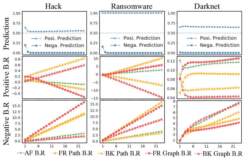
Figure 7. Prediction evolution of different address groups and corresponding average Benevolent Rates (B.R) of different features.

To verify the effectiveness and versatility of our Evolve Path Tracer, we first compare the most common machine learning models, then compare our encoder module with the encoder in other early detection models. At last, we also compare the address graph-based models. The models are detailed in the appendix. The main results for comparing all different methods are shown in Table 2, and the major findings are summarized as follows:

(1) Our Evolve Path Tracer outperforms most compared methods by a significant margin. Especially for early detection performance metrics F1-E and F1-C, Evolve Path Tracer achieves the best performance under all three datasets. Compared to the second-best methods, Evolve Path Tracer has an average increase of $14.54$% on $F1^{E}$ and an average increase of $15.63$% on $F1^{C}$. Besides, none of these methods can perform well on all three datasets, which justifies the effectiveness and versatility of our Evolve Path Tracer. Besides, the ”Early Stop” mechanism accelerates the prediction speed and helps the model to discard subsequent noise.

(2) Traditional machine learning algorithms do not perform well on the three datasets. It is difficult for decision-tree-based machine learning algorithms to encode the temporal shifts of the decision boundary for different features (Masud et al., 2011, 2013). Therefore, our model has an average improvement of $80.52$% on $F1^{E}$ and $83.44$% on $F1^{C}$ compared to the best decision-tree-based model.

(3) The sequential methods perform well on the three datasets. However, our Evolve Path Tracer still has an average $21.82$% improvement on $F1^{E}$ and $24.11$% on $F1^{C}$ compared to the best model in this group. The first reason is that the inter-relationships among asset transfer paths can reveal specific transaction patterns (e.g., two addresses transfer money through multiple paths to avoid monitoring). In addition, since the transaction pattern evolves in the early stage, a static encoding module can hardly encode evolving information.

(4) Compared with Address Graph methods, Evolve Path Tracer has average increases of $22.74$% and $23.36$% on $F1^{E}$ and $F1^{C}$ respectively. Among them, Evolve-GCN performs the best in most datasets, which verifies the fast-evolving of early transaction networks. However, as (Liu et al., 2021) implies, the address GCN may lead to Over-Smoothing issues and the dilution of the minority class. Moreover, as most neighbors of malicious nodes are victims or shadow addresses, the Address Graph models do not perform well. To avoid these problems, in Evolve Path Tracer, we set vertices as transactions to utilize the relevant address information in a ”safer” way.

6.5. Ablation Study (RQ3)

As shown in Table 3, AF performed poorly on the three datasets. Because many benevolent addresses (change address, ICO, and legal market addresses) behave similarly to these malicious addresses. As shown in Fig. 7, the AF benevolent rates for most negative samples do not exceed 2.5. The introduction of asset transfer path features significantly improves the performance. As shown in Fig. 7, for the Hack addresses, the forward transaction signal is more important than the backward one because the Hack address will transfer the funds faster and more centralized. Ransomware and Darknet addresses usually require victims or buyers to transfer funds according to certain conditions, the backward information is thus more critical.

Comparing +Path and +Graph, by encoding the paths’ interrelationships, the model gives predictions based on transaction patterns rather than the fluctuation of a single path. As shown in Fig. 7, the prominent signals of malicious nodes are enhanced by introducing path graphs. In the cryptocurrency transaction network, the model should be able to handle the differences between various types of addresses dynamically. By comparing the performance differences between +Graph and +Evolve, we found that this Evolve mechanism is necessary. +Graph only performs well if the address has a shorter life span, and these addresses will be discarded after the first few transactions. However, for other addresses with longer lifetimes, +Evolve can better reflect changes in the transaction patterns of these addresses, resulting in better performance.

6.6. Scalability and Dynamical Prediction (RQ4)

Feature Preparation Time Cost. When a new block appears, users will usually monitor the addresses that have transactions with them. Those new and large-volume addresses are likely to participate in dangerous activities. Therefore, we randomly selected $1,000$ blocks (from the first block of $2018$ to the first block of $2022$) and collected the daily BTC price during this period. We filter out transactions lower than $$10,000$ and retrieve addresses with a lifespan of less than one week. We prepare every address’s data for the first $24$ hours, the time cost is illustrated in Table 6.

Table 4. Time cost of different input data, including Block Number, Transaction Number, Address Number), Address Feature, Asset Transfer Path, Path Graph, and Address Graph.

#Blk	#TX	#Addr	A-Feat	Path	P-G	A-G
1,000	306,258	194,310	175s	7.7h	6.9h	14.3h
Avg.	306	194	0.2s	27.6s	24.8s	51.4s

During each interval (1 hour is about $6$ blocks), we need to monitor about $1,166$ new addresses, which will only cost 5 minutes. Moreover, as shown in Table 6, our time cost resembles address graph preparation, but we can collect information much further than $2$ hops.

Scalability of Early Stop. We plot the skip ratios with different thresholds to justify the scalability. As shown in Fig. 8, all models can filter out most ($80$%) addresses by the fourth hour. The mechanism improves the model’s Scalability significantly. Moreover, a reasonable threshold helps the model to discard subsequent noise and improve the performance, as mentioned in Section 6.4. A lower threshold means a faster prediction speed. Inf means no “Early Stop” mechanism, the skip ratio is thus always $0$.

There is a concern about missing malicious addresses as we decrease the threshold, which then decreases the model’s Recall scores. However, as shown in Fig. 8, compared to the model without “Early Stop” (labeled as “Inf”), the model has better Recall scores as we decrease the threshold. This is because our model can predict the most benevolent addresses in the early hours. Removing them from the monitoring list can avoid subsequent noise, which improves the model’s Recall scores. Therefore, our Evolve Path Tracer has a faster prediction speed without missing malicious addresses.

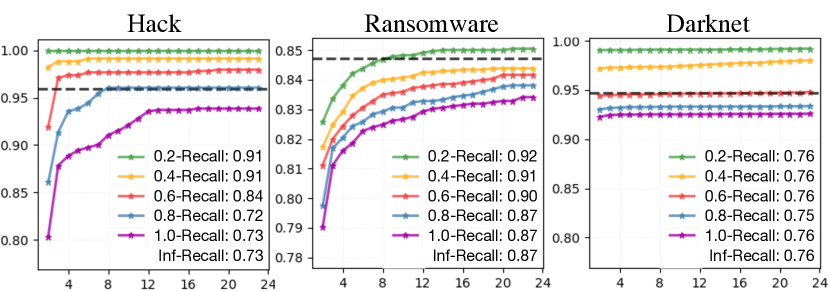
Figure 8. Skip Ratio evolution and $Recall$ scores with different thresholds. The gray line is the benevolent ratio of each dataset.

7. Conclusion and Future Work

In this paper, we present Evolve Path Tracer, a novel framework for early malicious address detection. We first propose Asset Transfer Paths and encode them with Evolve Path Encoder LSTM. The asset transfer paths exhibit high versatility in monitoring various transaction patterns in the early stage. Then the Evolve Path Graph GCN is built to encode corresponding path graphs. The graphs capture the interrelation among the paths. In particular, all modules are evolving dynamically to encode the dynamics of paths’ structure and inter-relation. Finally, we implement Hierarchical Survival Predictor with Consistency Loss Function to achieve better prediction performance, higher consistency, and excellent scalability. The model is comprehensively evaluated on three datasets. Extensive ablation studies explain the mechanisms behind the effectiveness and excellent scalability.

8. Acknowledgments

This research is supported by the National Research Foundation, Singapore under its Emerging Areas Research Projects (EARP) Funding Initiative, the NSFC (72171071, 72271084, 72101079) and the Excellent Fund of HFUT (JZ2021HGPA0060). Any opinions, findings and conclusions or recommendations expressed in this material are those of the author(s) and do not reflect the views of National Research Foundation, Singapore.

Appendix A Supplementary Material

A.1. Reproducibility

We first download full-node BTC raw data with Bitcoin Core. The whole data size is about 500GB. After downloading all blocks before the 700,000th block, we parse all data by Blocksci for querying block, transaction, and address index. The parsed data size is about 400GB. For each address in our dataset, we prepare its asset transfer paths for the transactions during the first 24 hours. The process was executed on AMD Ryzen 9 3900X Processor with 64GB of memory. We implement Evolve Path Tracer in Pytorch and Geometric. All experiments are conducted on a single NVIDIA RTX 2080TI with 11GB memory. The dimension of hidden layers in our model is 32, with a total of 919203 ( 0.9M) parameters. The size of the model’s checkpoint is only 3.57 MB. The training was performed for a maximum of 40 epochs. Early stopping is applied if the best performance didn’t update in the latest five epochs. The training and testing time cost for each dataset is shown in Table. 6:

Table 5. Key components and module description. TX stands for the transaction. BK and FR stand for Backward and Forward.

Name(Notation)	Description
Influence TX pair ($j\rightarrow i$)	A certain portions of TX i’s BTCs come from TX j
Trust TX pair ($i\rightarrow j$)	A certain portions of TX i’s BTCs flow to TX j
BK Asset Transfer Path ($j_{n}\rightarrow\cdots\rightarrow i$)	Build the Influence TX pairs iteratively and link them to form a path
FR Asset Transfer Path ($i\rightarrow\cdots\rightarrow j_{n}$)	Build the Trust TX pairs iteratively and link them to form a path
BK/FR Path Graph	BK/FR Asset Transfer paths share the same source/destination TX are grouped to form a graph
T-1 LSTM	LSTM to encode temporal information of address features
E-1/2 LSTM	An Evolve Path Encoder LSTM for encoding BK/FR Asset Transfer Path to Path feature
T-2/3 LSTM	LSTM to encode temporal information of BK/FR Path feature
BK/FR-Graph Encoder	An Evolve Path Graph GCN for encoding BK/FR Path Graph to Graph feature
T-4/5 LSTM	LSTM to encode temporal information of BK/FR Graph feature

Table 6. Time Cost

Type	Train	Test	Time-Span	Sample Num.
H	0.6 hours	0.6 mins	24 hours	6,884
R	1.1 hours	2.3 mins	24 hours	24,324
D	7.6 hours	16.3 mins	24 hours	115,775

Figure 9. Asset transfer path’s statistical properties of different malicious addresses under the backward and forward direction.

A.2. Label Acquisition

To get the labels for three different illicit activities (Hack, Ransomware, and Darknet), we performed a manual search on public forums and datasets, such as Bitcointalk forum, Reddit, WalletExplorer and several prior studies (Paquet-Clouston et al., 2019; Li et al., 2020; Wu et al., 2021). Negative (Regular) addresses are collected in the same method as  (Wu et al., 2021; Liu et al., 2003). We set the activation threshold as $0.01$ to prepare the asset transfer path. One can set a smaller threshold depending on the operating environment.

A.3. Address Features

We use the following features to characterize an address at a specific timestamp.

• the current balance of the address

• the number of receive (spend) transactions,

• the ratio of receiving (spend) transactions number,

• the maximum receive (spend) transactions number,

• the life span of the address,

• address active rate.

A.4. Transaction Features

We use the following features to characterize a transaction, which is the component of every asset transfer path.

• the height interval to the path source,

• the influence (trust) score with the previous transaction,

• the input amount of the previous transaction,

• the transaction fee,

• the total amount (resp. max, min, avg, and var) of all receive (spend) transactions,

• the number of receive (spend) transactions.

A.5. Preparation of Asset Transfer Path

Algo. 1 gives the detail to prepare Backward Asset Transfer Paths that reveal where $j$ obtains the asset. The pipeline to construct Forward Asset Transfer Path is similar to Backward Asset Transfer Path. The only difference is the tracing direction. The essence of each node is a transaction, so we use a sequence of transaction features to represent an asset transfer path.

input : Initial Output Tx $j^{o}$, Threshold $\theta$, Time Span $T_{Span}$.

output : Backward Path Set $P$.

1Initialize Backward Path Set: $P\leftarrow\{[-,1,j^{o}]\}$;

2 Initialize Previous hop recorder: $P_{pre}\leftarrow\{[-,1,j^{o}]\}$;

3 Initialize Ending Flag: $F_{end}\leftarrow False$;

4 $j^{o}$’s Time: $T_{j^{o}}\leftarrow$ Time of $j^{o}$;

5while $F_{end}\neq True$ do

      6 Current hop recorder $P_{now}\leftarrow\{\}$;

      7 $F_{end}\leftarrow True$;

      8 for $p$ in $P_{pre}$ do

            9 $j\leftarrow$ Output Tx $p[2]$;

            10 $I\leftarrow$ Input Tx Set of $j$;

            11 for $i$ in $I$ do

                  12 $Prop_{i}\leftarrow Amt_{i}/Amt_{I}$;

                  13 $Score_{i}\leftarrow Prop_{i}*p[1]$;

                  14 $T_{i}\leftarrow$ time of $i$;

                  15 if ($Score_{i}\geq\theta$ and $T_{j^{o}}-T_{i}\leq T_{Span}$) then

                        16 Append $[j,Score_{i},i]$ to $P_{now}$;

                        17 $F_{end}\leftarrow F_{end}$ $\&\&$ $False$;

                  

            

      18$P_{pre}\leftarrow P_{now}$;

      19 $P\leftarrow P\cup P_{pre}$;

      

20return $P$

Algorithm 1 Backward Path Preparation

A.6. Baseline Models

We give details of our baseline methods from two related tasks:

Malicious Detection in Cryptocurrency. We compare Evolve Path-Tracer with several models for malicious address detection in cryptocurrencies. For decision tree models, we use address features and path statistic features as the feature set. For GCN models, at each time step, we get the addresses’ embedding after two graph convolutional layers as implemented in  (Weber et al., 2019). Then, we feed the embeddings into a sequential model for prediction.

• Decision Tree (Liang et al., 2019; Nerurkar et al., 2020) utilize Decision Tree for identifying these malicious addresses.

• Random Forest (Nerurkar et al., 2020) utilize Decision Tree for identifying these malicious addresses.

• XGB (Harlev et al., 2018b; Nerurkar et al., 2020) predict the type of a yet-unidentified entity with Gradient Boosting based algorithms.

• GCN (Weber et al., 2019) encodes the objective address based on its transaction address graph.

• Skip-GCN (Weber et al., 2019) inserts a skip connection between the intermediate embedding and the input node features.

• Evolve-GCN (Weber et al., 2019) updates GCN weights with an RNN module.

Early Rumor Detection on Social Media. For these sequential models, we build an extra path LSTM encoder for a fair comparison. We concatenate address features with the path-encoder output and feed them into the sequential prediction model.

• GRU (Cho et al., 2014) is a typical neural network for sequence modeling. At each time split, previous hidden state and current summation features are fed into the GRU unit to predict the labels for the given addresses.

• M-LSTM (Yuan et al., 2017) adopts LSTM for every kind of feature to generate its own temporal features at each timestamp. Here we build three LSTM models for Address Features, Forward Paths, and Backward Paths.

• CED (Song et al., 2019) also uses GRU for sequence modeling, it proposes the concept of “Credible Detection Point,” making it possible to make predictions as early as possible dynamically.

• SAFE (Zheng et al., 2019) adopts survival probability as the prediction. Instead of predicting the labels directly, it generates hazard rates for the survival models. The positive samples (Malicious Addresses) should die out fast, while the negative samples (Regular Addresses) should stay alive.

• TMIF  (Lv et al., 2022) is a transformer-based multi-modal mode to capture the dependency relationship between multi-modal content. Here we set the modal to be Address-Modal and Path-Modal.

References

- (1)
- Akcora et al. (2020) Cuneyt G Akcora, Yitao Li, Yulia R Gel, and Murat Kantarcioglu. 2020. Bitcoinheist: Topological data analysis for ransomware prediction on the bitcoin blockchain. In Proceedings of the twenty-ninth international joint conference on artificial intelligence.
- Al-rimy et al. (2019) Bander Ali Saleh Al-rimy, Mohd Aizaini Maarof, and Syed Zainudeen Mohd Shaid. 2019. Crypto-ransomware early detection model using novel incremental bagging with enhanced semi-random subspace selection. Future Generation Computer Systems 101 (2019), 476–491.
- Androulaki et al. (2013) Elli Androulaki, Ghassan O Karame, Marc Roeschlin, Tobias Scherer, and Srdjan Capkun. 2013. Evaluating user privacy in bitcoin. In International conference on financial cryptography and data security. Springer, 34–51.
- Chai et al. (2022) Ziwei Chai, Siqi You, Yang Yang, Shiliang Pu, Jiarong Xu, Haoyang Cai, and Weihao Jiang. 2022. Can Abnormality be Detected by Graph Neural Networks?. In Proceedings of the Twenty-Ninth International Joint Conference on Artificial Intelligence (IJCAI), Vienna, Austria. 23–29.
- Chen et al. (2020) Liang Chen, Jiaying Peng, Yang Liu, Jintang Li, Fenfang Xie, and Zibin Zheng. 2020. Phishing scams detection in ethereum transaction network. ACM Transactions on Internet Technology (TOIT) 21, 1 (2020), 1–16.
- Chen et al. (2019) Qian Chen, Sheikh Rabiul Islam, Henry Haswell, and Robert A Bridges. 2019. Automated ransomware behavior analysis: Pattern extraction and early detection. In International Conference on Science of Cyber Security. Springer, 199–214.
- Chen and Tsourakakis (2022) Tianyi Chen and Charalampos Tsourakakis. 2022. Antibenford subgraphs: Unsupervised anomaly detection in financial networks. In Proceedings of the 28th ACM SIGKDD Conference on Knowledge Discovery and Data Mining. 2762–2770.
- Cho et al. (2014) Kyunghyun Cho, Bart van Merriënboer, Dzmitry Bahdanau, and Yoshua Bengio. 2014. On the Properties of Neural Machine Translation: Encoder–Decoder Approaches. In Proceedings of SSST-8, Eighth Workshop on Syntax, Semantics and Structure in Statistical Translation. 103–111.
- Gutflaish et al. (2019) Eyal Gutflaish, Aryeh Kontorovich, Sivan Sabato, Ofer Biller, and Oded Sofer. 2019. Temporal anomaly detection: calibrating the surprise. In Proceedings of the AAAI Conference on Artificial Intelligence, Vol. 33. 3755–3762.
- Harlev et al. (2018a) Mikkel Alexander Harlev, Haohua Sun Yin, Klaus Christian Langenheldt, Raghava Mukkamala, and Ravi Vatrapu. 2018a. Breaking bad: De-anonymising entity types on the bitcoin blockchain using supervised machine learning. In Proceedings of the 51st Hawaii International Conference on System Sciences.
- Harlev et al. (2018b) Mikkel Alexander Harlev, Haohua Sun Yin, Klaus Christian Langenheldt, Raghava Mukkamala, and Ravi Vatrapu. 2018b. Breaking bad: De-anonymising entity types on the bitcoin blockchain using supervised machine learning. In Proceedings of the 51st Hawaii international conference on system sciences.
- Jiang et al. (2022) Shuli Jiang, Robson Leonardo Ferreira Cordeiro, and Leman Akoglu. 2022. D. MCA: Outlier Detection with Explicit Micro-Cluster Assignments. arXiv preprint arXiv:2210.08212 (2022).
- Jourdan et al. (2018) Marc Jourdan, Sebastien Blandin, Laura Wynter, and Pralhad Deshpande. 2018. Characterizing entities in the bitcoin blockchain. In 2018 IEEE international conference on data mining workshops (ICDMW). IEEE, 55–62.
- Kalodner et al. (2020) Harry Kalodner, Malte Möser, Kevin Lee, Steven Goldfeder, Martin Plattner, Alishah Chator, and Arvind Narayanan. 2020. Blocksci: Design and applications of a blockchain analysis platform. In 29th USENIX Security Symposium (USENIX Security 20). 2721–2738.
- Kuck et al. (2015) Jonathan Kuck, Honglei Zhuang, Xifeng Yan, Hasan Cam, and Jiawei Han. 2015. Query-based outlier detection in heterogeneous information networks. In Advances in database technology: proceedings. International Conference on Extending Database Technology, Vol. 2015. NIH Public Access, 325.
- Li et al. (2022) Sijia Li, Gaopeng Gou, Chang Liu, Chengshang Hou, Zhenzhen Li, and Gang Xiong. 2022. TTAGN: Temporal Transaction Aggregation Graph Network for Ethereum Phishing Scams Detection. In Proceedings of the ACM Web Conference 2022. 661–669.
- Li et al. (2020) Yang Li, Yue Cai, Hao Tian, Gengsheng Xue, and Zibin Zheng. 2020. Identifying illicit addresses in bitcoin network. In International Conference on Blockchain and Trustworthy Systems. Springer, 99–111.
- Liang et al. (2019) Jiaqi Liang, Linjing Li, Daniel Zeng, Shu Luan, and Lu Gan. 2019. Bitcoin exchange addresses identification and its application in online drug trading regulation. (2019).
- Lin et al. (2020) Dan Lin, Jiajing Wu, Qi Yuan, and Zibin Zheng. 2020. T-edge: Temporal weighted multidigraph embedding for ethereum transaction network analysis. Frontiers in Physics 8 (2020), 204.
- Liu et al. (2003) Bing Liu, Yang Dai, Xiaoli Li, Wee Sun Lee, and Philip S Yu. 2003. Building text classifiers using positive and unlabeled examples. In Third IEEE International Conference on Data Mining. IEEE, 179–186.
- Liu et al. (2021) Yang Liu, Xiang Ao, Zidi Qin, Jianfeng Chi, Jinghua Feng, Hao Yang, and Qing He. 2021. Pick and Choose: A GNN-Based Imbalanced Learning Approach for Fraud Detection. In Proceedings of the Web Conference 2021.
- Lv et al. (2022) Jiandong Lv, Xingang Wang, and Cuiling Shao. 2022. TMIF: transformer-based multi-modal interactive fusion for automatic rumor detection. Multimedia Systems (2022), 1–11.
- Masud et al. (2011) Mohammad Masud, Jing Gao, Latifur Khan, Jiawei Han, and Bhavani M. Thuraisingham. 2011. Classification and Novel Class Detection in Concept-Drifting Data Streams under Time Constraints. IEEE Transactions on Knowledge and Data Engineering 23, 6 (2011), 859–874. https://doi.org/10.1109/TKDE.2010.61
- Masud et al. (2013) Mohammad M. Masud, Qing Chen, Latifur Khan, Charu C. Aggarwal, Jing Gao, Jiawei Han, Ashok Srivastava, and Nikunj C. Oza. 2013. Classification and Adaptive Novel Class Detection of Feature-Evolving Data Streams. IEEE Transactions on Knowledge and Data Engineering 25, 7 (2013), 1484–1497. https://doi.org/10.1109/TKDE.2012.109
- Nerurkar et al. (2020) Pranav Nerurkar, Yann Busnel, Romaric Ludinard, Kunjal Shah, Sunil Bhirud, and Dhiren Patel. 2020. Detecting illicit entities in bitcoin using supervised learning of ensemble decision trees. In Proceedings of the 2020 10th international conference on information communication and management. 25–30.
- Paquet-Clouston et al. (2019) Masarah Paquet-Clouston, Bernhard Haslhofer, and Benoit Dupont. 2019. Ransomware payments in the bitcoin ecosystem. Journal of Cybersecurity 5, 1 (2019).
- Pareja et al. (2020) Aldo Pareja, Giacomo Domeniconi, Jie Chen, Tengfei Ma, Toyotaro Suzumura, Hiroki Kanezashi, Tim Kaler, Tao Schardl, and Charles Leiserson. 2020. Evolvegcn: Evolving graph convolutional networks for dynamic graphs. In Proceedings of the AAAI Conference on Artificial Intelligence, Vol. 34. 5363–5370.
- Reid and Harrigan (2013) Fergal Reid and Martin Harrigan. 2013. An analysis of anonymity in the bitcoin system. In Security and privacy in social networks. Springer, 197–223.
- Roy and Chen (2021) Krishna Chandra Roy and Qian Chen. 2021. Deepran: Attention-based bilstm and crf for ransomware early detection and classification. Information Systems Frontiers 23, 2 (2021), 299–315.
- Shao et al. (2018) Wei Shao, Hang Li, Mengqi Chen, Chunfu Jia, Chunbo Liu, and Zhi Wang. 2018. Identifying bitcoin users using deep neural network. In International Conference on Algorithms and Architectures for Parallel Processing. Springer, 178–192.
- Song et al. (2019) Changhe Song, Cheng Yang, Huimin Chen, Cunchao Tu, Zhiyuan Liu, and Maosong Sun. 2019. CED: Credible early detection of social media rumors. IEEE Transactions on Knowledge and Data Engineering (2019).
- Sun et al. (2012) Yizhou Sun, Jiawei Han, Charu C. Aggarwal, and Nitesh V. Chawla. 2012. When Will It Happen? Relationship Prediction in Heterogeneous Information Networks. In Proceedings of the Fifth ACM International Conference on Web Search and Data Mining (WSDM ’12). 663–672. https://doi.org/10.1145/2124295.2124373
- Tam et al. (2019) Da Sun Handason Tam, Wing Cheong Lau, Bin Hu, Qiu Fang Ying, Dah Ming Chiu, and Hong Liu. 2019. Identifying Illicit Accounts in Large Scale E-payment Networks–A Graph Representation Learning Approach. arXiv preprint arXiv:1906.05546 (2019).
- Tang et al. (2022) Jianheng Tang, Jiajin Li, Ziqi Gao, and Jia Li. 2022. Rethinking graph neural networks for anomaly detection. In International Conference on Machine Learning. PMLR, 21076–21089.
- Vasek and Moore (2015) Marie Vasek and Tyler Moore. 2015. There’s no free lunch, even using Bitcoin: Tracking the popularity and profits of virtual currency scams. In International conference on financial cryptography and data security. Springer, 44–61.
- Weber et al. (2019) Mark Weber, Giacomo Domeniconi, Jie Chen, Daniel Karl I Weidele, Claudio Bellei, Tom Robinson, and Charles E Leiserson. 2019. Anti-money laundering in bitcoin: Experimenting with graph convolutional networks for financial forensics. arXiv preprint arXiv:1908.02591 (2019).
- Wu et al. (2021) Jiajing Wu, Jieli Liu, Weili Chen, Huawei Huang, Zibin Zheng, and Yan Zhang. 2021. Detecting mixing services via mining bitcoin transaction network with hybrid motifs. IEEE Transactions on Systems, Man, and Cybernetics: Systems (2021).
- Wu et al. (2020) Jiajing Wu, Qi Yuan, Dan Lin, Wei You, Weili Chen, Chuan Chen, and Zibin Zheng. 2020. Who are the phishers? phishing scam detection on ethereum via network embedding. IEEE Transactions on Systems, Man, and Cybernetics: Systems (2020).
- Yin and Vatrapu (2017) Haohua Sun Yin and Ravi Vatrapu. 2017. A first estimation of the proportion of cybercriminal entities in the bitcoin ecosystem using supervised machine learning. In 2017 IEEE International Conference on Big Data (Big Data). IEEE, 3690–3699.
- Yuan et al. (2017) Shuhan Yuan, Panpan Zheng, Xintao Wu, and Yang Xiang. 2017. Wikipedia vandal early detection: from user behavior to user embedding. In Joint European Conference on Machine Learning and Knowledge Discovery in Databases. Springer, 832–846.
- Zhang et al. (2022) Ge Zhang, Zhenyu Yang, Jia Wu, Jian Yang, Shan Xue, Hao Peng, Jianlin Su, Chuan Zhou, Quan Z Sheng, Leman Akoglu, et al. 2022. Dual-discriminative Graph Neural Network for Imbalanced Graph-level Anomaly Detection. In Advances in Neural Information Processing Systems.
- Zhang et al. (2017) Jiawei Zhang, Congying Xia, Chenwei Zhang, Limeng Cui, Yanjie Fu, and S Yu Philip. 2017. BL-MNE: emerging heterogeneous social network embedding through broad learning with aligned autoencoder. In 2017 IEEE International Conference on Data Mining (ICDM). IEEE, 605–614.
- Zhao et al. (2022) Lingxiao Zhao, Saurabh Sawlani, Arvind Srinivasan, and Leman Akoglu. 2022. Graph Anomaly Detection with Unsupervised GNNs. https://doi.org/10.48550/ARXIV.2210.09535
- Zheng et al. (2019) Panpan Zheng, Shuhan Yuan, and Xintao Wu. 2019. Safe: A neural survival analysis model for fraud early detection. In Proceedings of the AAAI Conference on Artificial Intelligence, Vol. 33. 1278–1285.