Multiple Populations in Low-mass Globular Clusters: Eridanus
Abstract
Multiple populations (MPs), characterized by variations in light elemental abundances, have been found in stellar clusters in the Milky Way, Magellanic Clouds, as well as several other dwarf galaxies. Based on a large amount of observations, mass has been suggested to be a key parameter affecting the presence and appearance of MPs in stellar clusters. To further investigate the existence of MPs in low-mass clusters and explore the mass threshold for MP formation, we carried out a project studying the stellar population composition in several low-mass Galactic globular clusters. Here we present our study on the cluster Eridanus. With blue-UV low-resolution spectra obtained with the OSIRIS/Multi-object spectrograph on the Gran Telescopio Canarias, we computed the spectral indices of CH and CN for the sample giant stars, and derived their carbon and nitrogen abundances using model spectra. A significant dispersion in the initial surface abundance of nitrogen was found in the sample, indicating the existence of MPs in Eridanus. Inspecting the age-initial mass distribution of in-situ clusters with MPs, we find a slight trend that initial mass increases with increasing age, and the lowest initial mass of 4.98 and 5.26 are found at the young and old end, respectively, which might provide a rough reference for the mass threshold for clusters to form MPs. However, more observations of clusters with low initial masses are still necessary before any firm conclusion can be drawn.
1 Introduction
Chemical abundance variations in light elements of globular clusters (GCs) were discovered half a century ago (Osborn, 1971). Besides “normal” stars with chemical abundances similar to field stars, the stars showing chemical anomalies, e.g., deficiency in carbon, oxygen, and magnesium; enrichment in helium, nitrogen, sodium, and aluminium, were discovered to commonly exist in GCs as well in series of observations, which are termed as “multiple populations” (MPs) (e.g., Gratton et al., 2004; Pancino et al., 2010; Carretta et al., 2010; Pancino et al., 2017; Masseron et al., 2019; Mészáros et al., 2020, and references there in). In addition to direct abundance analysis using spectra, photometry is also an effective way to study MPs, especially for faint clusters where high signal to noise ratio (SNR) spectra are unreachable. MP studies through photometry mainly use nitrogen-related molecular absorption bands in the UV-blue portion of the spectrum (e.g., NH, CN) (e.g., Piotto et al., 2012, 2015; Milone et al., 2017).
Although the existence of MPs is currently well accepted as a general feature for GCs, theoretical explanations for its origin have not reached a consensus (see Bastian & Lardo, 2018, and references therein). Under the hypothesis of self-enrichment, which has been widely recognized, the ashes of high-temperature hydrogen burning were ejected from massive primordial stars and mixed with interstellar medium. Then enriched stars that formed out of the mixture should show the enriched chemical pattern/chemical anomalies. The nature of the polluters has been debated for almost two decades, e.g., massive AGB stars (D’Ercole et al., 2010; Ventura & D’Antona, 2011), fast-rotating massive stars (Decressin et al., 2007b, a), supermassive stars (Denissenkov & Hartwick, 2014; Denissenkov et al., 2015), massive interacting binaries (de Mink et al., 2009) and stellar mergers (Wang et al., 2020). However, none of the popular scenarios can reproduce the complex observed phenomena (Renzini et al., 2015; Bastian & Lardo, 2018).
After inspection of a large number of GCs, cluster mass, metallicity and age are found to be the key parameters affecting the presence of MPs (Carretta et al., 2010; Bastian & Lardo, 2018). To provide threshold parameters that can discriminate between and improve existing formation models, it is vital to investigate the detailed manifestation of MPs at critical conditions. For example, at the metal-rich end, NGC 6553 was found to be the most metal-rich GC with MPs, suggesting a potential metallicity ([Fe/H]) upper limit of -0.15 (Tang et al., 2017). In term of cluster age, no clusters with ages younger than 2 Gyr have been found to host MPs so far, thus 2 Gyr seems to be a lower limit of MP formation (Bastian & Lardo, 2018, and references therein).
Cluster mass has been suggested to be a universal parameter that decides the complexity of MPs, e.g., more massive clusters have larger abundance variations and fractions of enriched populations (Bastian & Lardo, 2018; Milone et al., 2020); more massive Type II GCs show larger iron spread (Milone & Marino, 2022). Exploring the critical cluster mass for MP formation will certainly enlighten the current MP scenarios. The possible mass boundary () proposed in Li et al. (2019) seems to well separate the intermediate-age GCs (2-10 Gyr) with and without MPs. But the situation is more complicated for older GCs. In this respect, NGC 6535 (mass = 2.2 ) was suspected to be the lowest-mass GC to harbor MPs based on high-resolution spectroscopy (Bragaglia et al., 2017), and moreover, MPs were found to probably exist in the lower-mass GC ESO452-SC11 (mass (6.8 3.4)) with low-resolution spectra (Simpson et al., 2017). Palomar 13 (Pal 13) was recently found to show MPs based on low-resolution spectra (Tang et al., 2021), and it could probably be the lowest-mass GC (mass , our most updated estimation) with MPs.
Under the hypothesis of self-enrichment, a minimum mass is indeed required by a cluster to retain ejecta from an initial generation and allow the formation of a subsequent generation, depending of course on the ejecta velocity. For example, from hydrodynamical simulations, Vesperini et al. (2010) and Bekki (2011) both found a lower mass limit, and , respectively, for stellar clusters to retain enough ejecta of primordial generation stars and form enriched generation stars. At the same time, the mass threshold has also been suggested by observations. Based on the Na-O anticorrelations, Carretta et al. (2010) showed that a minimum present-day mass of a few was required for stellar clusters to present MPs. Conroy & Spergel (2011) found that in the Large Magellanic Cloud (LMC) only clusters more massive than about showed MPs, and this critical mass was also consistent with their model prediction of the mass at which ram pressure was sufficient to remove the gas within the cluster. Moreover, Milone et al. (2020) suggested a threshold of in initial mass for Galactic GCs to form MPs, while clusters in the Magellanic Clouds seemed not to follow this limit.
Although several papers have proposed possible mass thresholds for stellar clusters to form MPs based on observations as mentioned above, no final conclusion can be derived until we have a comprehensive knowledge about the stellar population composition of low-mass clusters. However, this is a challenging work since low-mass clusters have few bright giant stars and are often located at large distances from the Sun. To take the study one step further and have a better understanding of the existence of MPs at the low-mass end, we have observed several low-mass Galactic GCs. Since they are remote objects, low-resolution spectra of their member stars were obtained to ensure enough signal-to-noise ratio (SNR) to derive the abundances of relevant species. As a subsequent work of our last study of MPs in Pal 13 (Tang et al., 2021), here we present the first study of the stellar population composition in the GC Eridanus, which has a present-day mass of (Baumgardt et al., 2019).
Eridanus was first discovered by Cesarsky et al. (1977). Having a metallicity of about [Fe/H] = -1.4 and distance of about 90 kpc (e.g., Harris, 1996, 2010 edition; see Sect. 3.1 for details), Eridanus is one of the most metal-rich clusters in the outer halo. With an age of 10.5 Gyr, it is also younger compared with inner-halo GCs at similar metallicities (Beccari et al., 2012). Hence, Eridanus is expected to have an external origin. Although being an interesting object for studies, it has not been explored spectroscopically, nor does its MP properties, due to its large Galactocentric distance. In this paper, we analyze the low-resolution spectra of Eridanus member stars to estimate their carbon and nitrogen abundances, searching for possible abundance variations that indicate MPs. In Section 2, we outline the observations and spectral reduction briefly. In Section 3, we analyze the spectra of member stars carefully and show our major results. The discussion and summary are given in Sections 4 and 5, respectively.
2 Observation and Data Reduction
2.1 Observation
The observations were carried out using the OSIRIS/Multi-object spectrograph (MOS) 111http://www.gtc.iac.es/instruments/osiris/osiris.php mounted on the Gran Telescopio Canarias (GTC), Observatorio del Roque de los Muchachos, under the program GTC2-18BCNT in December of 2018. The sample stars for observation were initially selected from the Gaia DR1 catalogue (Gaia Collaboration et al., 2016) by coordinates within the region of Eridanus GC. Given that slitlet observation forbids two targets from overlapping in the dispersion direction and brighter targets generate higher SNR spectra within a given time, 19 member stars were finally observed (Section 3). The observation consists of five observing blocks (OBs) with a total exposure time of 4.88 hours (See Table 1). Using R2500U as the dispersion element, the obtained spectra cover the wavelength range of 35004600 Å with nominal spectral resolution of 2500.
| observing block | date | exposure time (s) | airmass | seeing (”) |
|---|---|---|---|---|
| OB02 | 2018-12-08 | 18002 | 1.70 | 1.2 |
| OB06 | 2018-12-08 | 18002 | 1.55 | 1.1 |
| OB07 | 2018-12-08 | 15802 | 1.58 | 1.0 |
| OB09 | 2018-12-10 | 18002 | 1.55 | 1.2 |
| OB10 | 2018-12-10 | 18002 | 1.62 | 1.2 |
2.2 Data Reduction
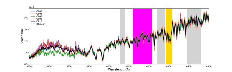
The data reduction was conducted following the procedure described in Tang et al. (2021), which can be summarized briefly as follows. The GTCMOS pipeline222https://www.inaoep.mx/ ydm/gtcmos/gtcmos.html was first used to complete basic steps: for each OB, the observed spectral images were bias-subtracted, combined, wavelength calibrated, flat-field corrected, and extracted to multiple one-dimension (1D) spectra. After velocity correction, the observed spectra were calibrated using model spectra in order to minimize the uncertainty caused by the flat-field correction. Considering the stellar parameters estimated in Section 3, we generated the model spectra with iSpec333https://www.blancocuaresma.com/s/iSpec (Blanco-Cuaresma et al., 2014; Blanco-Cuaresma, 2019), where the SPECTRUM radiative transfer code and line list, MARCS model atmospheres (Gustafsson et al., 2008) and the solar abundances from Asplund et al. (2005) were adopted. After the calibration, the spectra of the five OBs were co-added for each star (Fig. 1).
3 Analysis and results
3.1 Basic information of stars
We updated the Gaia photometry with Gaia DR2 data, and extinctions in G, BP and RP bands were computed using the coefficients provided by the team (Gaia Collaboration et al., 2018a). We also cross-matched the sample stars with the catalogue of Muñoz et al. (2018) to obtain their g and r band magnitudes. For the two stars (eri08 and eri10) that did not get matched, we supplemented their g and r band magnitudes by transforming from the Gaia photometry with the photometric relations provided in the “Gaia Data Release 2 Documentation release 1.2”444https://gea.esac.esa.int/archive/documentation/GDR2/Data_processing/chap_cu5pho/sec_cu5pho_calibr/ssec_cu5pho_PhotTransf.html. The systematic differences between the magnitudes of Muñoz et al. (2018) and those transformed from Gaia photometry were corrected based on other sample stars. Moreover, V and K band magnitudes were also computed for the sample stars from Gaia photometry. All the photometric magnitudes under consideration are listed in Table 2.
| ID | RA (J2000) | Dec (J2000) | G | e_G | BP | e_BP | RP | e_RP | g | e_g | r | e_r | pmRA | e_pmRA | pmDec | e_pmDec | Evol. phase |
|---|---|---|---|---|---|---|---|---|---|---|---|---|---|---|---|---|---|
| (mag) | (mag) | (mag) | (mag) | (mag) | (mag) | (mag) | (mag) | (mag) | (mag) | (mas/yr) | (mas/yr) | (mas/yr) | (mas/yr) | ||||
| eri01 | 66.176910 | -21.167276 | 19.650 | 0.005 | 19.992 | 0.054 | 18.885 | 0.030 | 20.215 | 0.003 | 19.560 | 0.003 | 1.1810 | 0.6248 | -0.8417 | 0.6942 | RGB |
| eri02 | 66.168472 | -21.170403 | 20.322 | 0.007 | 20.602 | 0.083 | 19.694 | 0.047 | 20.809 | 0.004 | 20.194 | 0.003 | -0.0457 | 1.0429 | 1.4722 | 1.2958 | RGB |
| eri03 | 66.182945 | -21.174185 | 18.013 | 0.002 | 18.687 | 0.018 | 17.251 | 0.009 | 18.872 | 0.002 | 17.946 | 0.002 | 0.7988 | 0.2064 | -0.1627 | 0.2227 | RGB |
| eri04 | 66.185150 | -21.175451 | 18.340 | 0.002 | 18.994 | 0.025 | 17.593 | 0.011 | 19.125 | 0.002 | 18.267 | 0.002 | 0.3653 | 0.2587 | -0.9767 | 0.2822 | RGB |
| eri05 | 66.173363 | -21.179552 | 18.407 | 0.002 | 18.984 | 0.021 | 17.652 | 0.014 | 19.178 | 0.002 | 18.332 | 0.002 | 0.5388 | 0.2920 | -0.4840 | 0.3129 | RGB |
| eri06 | 66.194931 | -21.180887 | 19.862 | 0.005 | 20.070 | 0.048 | 19.231 | 0.062 | 20.263 | 0.003 | 19.782 | 0.003 | -0.5298 | 0.8228 | 0.4895 | 0.7989 | HB |
| eri07 | 66.184982 | -21.181849 | 18.773 | 0.003 | 19.252 | 0.028 | 18.107 | 0.020 | 19.390 | 0.002 | 18.696 | 0.002 | 0.7575 | 0.3397 | -0.5467 | 0.3856 | AGB |
| eri08 | 66.183861 | -21.183519 | 17.328 | 0.002 | 17.876 | 0.012 | 16.388 | 0.006 | 18.309 | 0.000 | 17.248 | 0.000 | 0.4355 | 0.1299 | -0.1746 | 0.1437 | RGB |
| eri09 | 66.181190 | -21.184744 | 18.068 | 0.002 | 18.680 | 0.020 | 17.290 | 0.009 | 18.895 | 0.002 | 17.999 | 0.002 | 0.7367 | 0.2031 | -1.0208 | 0.2285 | RGB |
| eri10 | 66.187309 | -21.185621 | 17.073 | 0.002 | 17.835 | 0.010 | 16.203 | 0.005 | 18.210 | 0.000 | 17.020 | 0.000 | 0.4044 | 0.1173 | -0.5422 | 0.1333 | RGB |
| eri11 | 66.188339 | -21.188213 | 19.143 | 0.003 | 19.450 | 0.035 | 18.369 | 0.025 | 19.691 | 0.003 | 19.050 | 0.003 | 0.5976 | 0.4182 | -0.9497 | 0.4862 | AGB |
| eri12 | 66.195686 | -21.189545 | 20.644 | 0.008 | 20.757 | 0.122 | 19.920 | 0.090 | 21.113 | 0.004 | 20.531 | 0.004 | 3.4233 | 1.5259 | -0.2365 | 1.3503 | RGB |
| eri13 | 66.185699 | -21.190716 | 20.558 | 0.009 | 20.512 | 0.082 | 19.853 | 0.095 | 20.997 | 0.005 | 20.415 | 0.004 | -0.2745 | 1.3342 | 2.3632 | 1.5846 | RGB |
| eri14 | 66.182388 | -21.191929 | 20.171 | 0.007 | 20.453 | 0.070 | 19.597 | 0.057 | 20.500 | 0.004 | 20.080 | 0.003 | 0.5595 | 0.9482 | -1.7182 | 1.2901 | HB |
| eri15 | 66.185364 | -21.195387 | 18.719 | 0.003 | 19.251 | 0.020 | 18.016 | 0.015 | 19.426 | 0.002 | 18.637 | 0.002 | 0.8461 | 0.3807 | -0.6992 | 0.3909 | RGB |
| eri16 | 66.186218 | -21.197334 | 20.149 | 0.006 | 20.312 | 0.050 | 19.496 | 0.038 | 20.493 | 0.003 | 20.081 | 0.003 | 0.0457 | 0.9189 | 2.1428 | 1.0991 | HB |
| eri17 | 66.177940 | -21.202587 | 18.988 | 0.003 | 19.528 | 0.025 | 18.262 | 0.019 | 19.642 | 0.002 | 18.903 | 0.002 | 0.3619 | 0.3844 | 0.0074 | 0.4424 | RGB |
| eri18 | 66.172325 | -21.141823 | 20.047 | 0.007 | 20.092 | 0.065 | 19.488 | 0.094 | 20.232 | 0.003 | 19.972 | 0.004 | -1.3608 | 0.6670 | -3.3207 | 0.8347 | HB |
| eri19 | 66.189949 | -21.221462 | 20.678 | 0.010 | 20.901 | 0.103 | 20.239 | 0.115 | 21.012 | 0.004 | 20.581 | 0.005 | 2.8056 | 1.6933 | -2.7386 | 2.0293 | HB |
Figure 2 shows the colormagnitude diagram (CMD) of Eridanus, where the photometric catalogue of Muñoz et al. (2018) is used. Grey dots indicate stars located within the tidal radius of (Myeong et al., 2017). Using grids of PARSEC isochrones to fit the CMD distribution, we determined the age of Eridanus to be 10.0 0.5 Gyr and metallicity to be -1.45 0.05 dex. The distance modulus and reddening E(g-r) were also derived as 19.83 0.04 mag and 0.025 0.010 mag, respectively. A distance of 92.47 1.71 kpc is then obtained based on the distance modulus. Considering the V-band magnitude 15.02 mag of Eridanus derived by Baumgardt et al. (2020), the absolute visual magnitude is = -4.81 mag. E(B-V) of 0.021 0.008 mag was derived adopting the extinction coefficients by McCall (2004). These parameters have also been determined in previous studies. For example, the metallicity of -1.350.2 dex, distance of 81 kpc to the Sun and absolute visual magnitude of -4.85 mag have been derived by Da Costa (1985) via CMD fitting for the first time. The distance of 90.1 kpc to the Sun by Stetson et al. (1999) and metallicity of -1.43 which is the average of the values by Armandroff & Da Costa (1991) and Carretta et al. (2009) are adopted by Harris (1996, 2010 edition) in the GC catalogue. Baumgardt & Vasiliev (2021) derived a distance of 84.68 kpc. An absolute age of 10.5 Gyr was obtained by Beccari et al. (2012) for this GC. For E(B-V), a weighted average value of 0.02 mag considering several sources is adopted by Harris (1996, 2010 edition), and Muñoz et al. (2018) determined it to be 0.018 mag. We conclude that our results of these parameters are consistent with those of previous works.
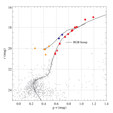
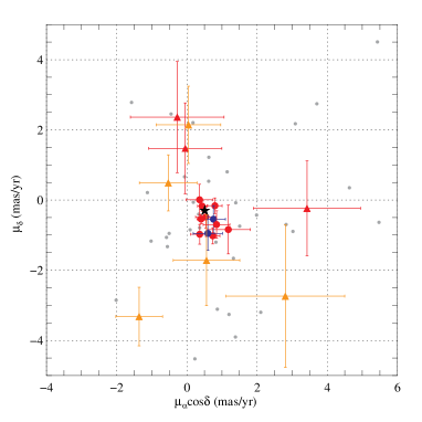
The stars that we observed are shown in Fig. 2 with large colored symbols. There are two AGB stars, 12 RGB stars555For two of these stars, it is difficult to distinguish between RGB or AGB based on their positions in CMD, but in our study we take them as RGB stars. and five HB stars (Table 2). We checked their proper motions from Gaia DR2 (Gaia Collaboration et al., 2018a) as shown in Fig. 3. All the HB stars and the faintest three RGB stars (represented by solid triangles in Figs. 2 and 3) have much larger uncertainties in their proper motions, compared with those brighter RGB and AGB stars (represented by solid circles). Since the G magnitudes of the fainter ones in our sample are about 20-21 mag, their uncertainties are comparable to the documented typical values (1.2-3 mas yr-1) at this magnitude range (Gaia Collaboration et al., 2018b).
3.2 Stellar parameters
The effective temperature () was first determined based on the Gaia photometry, considering the colortemperature relations provided in Mucciarelli & Bellazzini (2020). Six relatively independent determinations of were computed based on the de-reddened colors of (BP-RP), (BP-G), (G-RP), (BP-K), (RP-K) and (G-K). Converting the de-reddened (g-r) color into the color (B-V) adopting the transformation provided by Jester et al. (2005), we also considered another group of based on the color (B-V), which was derived using the colortemperature relation provided in González Hernández & Bonifacio (2009). The final was determined as the mean value of all the above seven values of after a sigma clipping. The associated errors were estimated taking the dispersions of the photometric calibrations and the uncertainties in the colour index and [Fe/H] into account. We estimated the stellar masses based on the isochrone (Table 3). Then, the surface gravities () were derived from , stellar masses, and bolometric luminosities. The relations of Alonso et al. (1999) were used to calculate the bolometric corrections.
Considering the derived of HB stars and the three faintest RGB stars (represented by solid triangles in Figs. 2 and 3) are all above 5500 K, the CN and CH molecular lines are weak for these hot stars; moreover, their uncertainties in proper motions are much larger than other brighter stars and their SNRs are substantially lower, we opted to neglect these hotter and fainter stars in the following analysis and discussion. In other words, we only consider the brighter RGB and AGB stars as our final sample. The derived , and their associated errors for each star in the final sample are listed in Table 3. The typical errors on and are about 50 K and 0.03 dex, respectively.
3.3 Spectral indices and abundances
Following the definition of Harbeck et al. (2003), we computed the spectral indices of CN4142 and CH4300 on the co-added calibrated spectra for each star.
| (1) |
| (2) |
where is the summed spectral flux from X to Y Å. Figure 1 shows the spectral regions for measuring the indices of CN4142 and CH4300. The errors of spectral indices were estimated mainly considering two factors, i.e., the errors of calibrating observed spectra with model spectra and the flux dispersion among calibrated OB spectra. Table 3 lists the derived spectral index values and their errors. Note that we did not plot CN versus CH (e.g., Gerber et al., 2020) here, because we do not have enough stars to define base lines where CN and CH.
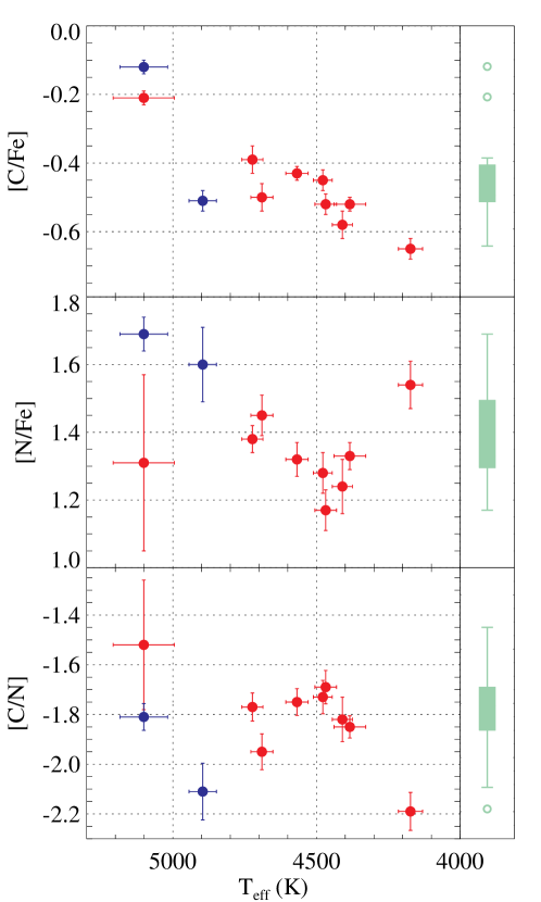
To analyze the [C/Fe] and [N/Fe] specifically, we took advantage of the model spectra from iSpec. For each star, we generated a grid of model spectra with [C/Fe and [N/Fe. [O/Fe] was assumed to be solar for all the model spectra.666 According to our test shown in Tang et al. (2021), the index differences for CN4142 and CH4300 caused by an [O/Fe] difference of 0.4 dex is almost negligible inside the discussed temperature range. The model spectral indices of CN4142 and CH4300 were computed for each model spectrum, so that the grid of model spectral indices was constructed for each star. By interpolation, we found the best match to the observed spectral indices from the model grid, so that a pair of best-match [C/Fe] and [N/Fe] was derived. In order to derive more reliable abundances as well as to estimate their errors, we performed the interpolation 1000 times for each star, considering variations in a Gaussian Monte Carlo approach in the input data. The mean abundances and their standard deviations are adopted as the final abundances of [C/Fe] and [N/Fe] and their errors, where the typical errors (median value) are 0.03 dex and 0.06 dex for [C/Fe] and [N/Fe], respectively. The results of the final sample stars are summarized in Table 3. By examining the dispersions () and the interquartile range (IQR) values of carbon and nitrogen abundances, which are = 0.15, IQR[C/Fe] = 0.11 and = 0.16, IQR[N/Fe] = 0.20, respectively, we find that the dispersions of [C/Fe] and [N/Fe] are similar and both significantly larger than their associated errors, while [C/Fe] distributes more concentratedly. These can also be detected visually in Fig. 4, which shows the distributions of [C/Fe] and [N/Fe], as well as the [C/N] ratio.
| ID | mass | e_ | e_ | CN4142 | e_CN4142 | CH4300 | e_CH4300 | [C/Fe] | e_[C/Fe] | [N/Fe] | e_[N/Fe] | ||
|---|---|---|---|---|---|---|---|---|---|---|---|---|---|
| () | (K) | (K) | |||||||||||
| eri01 | 0.847 | 5101 | 106.58 | 2.15 | 0.05 | -0.017 | 0.007 | 0.209 | 0.005 | -0.21 | 0.02 | 1.31 | 0.26 |
| eri03 | 0.836 | 4410 | 35.14 | 1.18 | 0.03 | -0.005 | 0.008 | 0.273 | 0.007 | -0.58 | 0.04 | 1.24 | 0.08 |
| eri04 | 0.839 | 4468 | 37.62 | 1.34 | 0.03 | -0.012 | 0.006 | 0.279 | 0.006 | -0.52 | 0.03 | 1.17 | 0.06 |
| eri05 | 0.840 | 4568 | 38.66 | 1.42 | 0.03 | 0.007 | 0.008 | 0.281 | 0.005 | -0.43 | 0.02 | 1.32 | 0.05 |
| eri07 | 0.780 | 4896 | 47.80 | 1.67 | 0.03 | 0.005 | 0.007 | 0.185 | 0.005 | -0.51 | 0.03 | 1.60 | 0.11 |
| eri08 | 0.828 | 4384 | 55.01 | 0.89 | 0.04 | 0.020 | 0.006 | 0.290 | 0.005 | -0.52 | 0.02 | 1.33 | 0.04 |
| eri09 | 0.837 | 4478 | 32.70 | 1.24 | 0.03 | 0.007 | 0.007 | 0.290 | 0.006 | -0.45 | 0.03 | 1.28 | 0.06 |
| eri10 | 0.819 | 4173 | 42.12 | 0.67 | 0.03 | 0.037 | 0.008 | 0.274 | 0.006 | -0.65 | 0.03 | 1.54 | 0.07 |
| eri11 | 0.790 | 5101 | 83.02 | 1.91 | 0.04 | 0.006 | 0.005 | 0.214 | 0.005 | -0.12 | 0.02 | 1.69 | 0.05 |
| eri15 | 0.842 | 4723 | 36.71 | 1.61 | 0.03 | -0.001 | 0.004 | 0.264 | 0.010 | -0.39 | 0.04 | 1.38 | 0.04 |
| eri17 | 0.844 | 4690 | 38.31 | 1.71 | 0.03 | 0.006 | 0.007 | 0.245 | 0.010 | -0.50 | 0.04 | 1.45 | 0.06 |
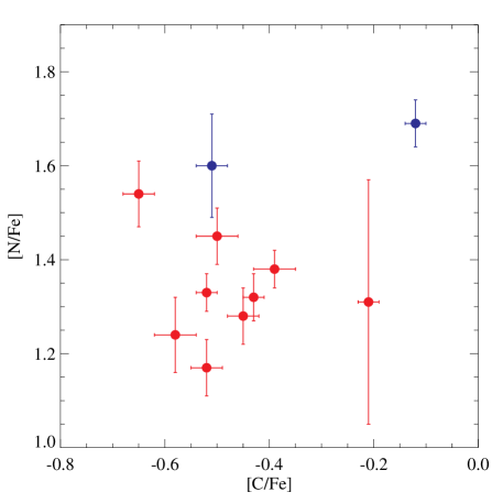
The activated CNO cycle in the cores of evolved low-mass stars may change the surface chemical abundances if the convective envelope reaches deep enough. As stars climb up the RGB, the surface abundances of carbon and nitrogen would be altered due to the first dredge-up and extra-mixing processes. Especially, the extra-mixing process can significantly change the surface abundances of stars brighter than the RGB bump (e.g., Gratton et al., 2000; Charbonnel & Zahn, 2007; Lagarde et al., 2012). As shown in Fig. 2, only the faintest RGB star in our final sample is located below the RGB bump, while all the others should have experienced the extra-mixing. So the abundance distributions shown in Fig. 4 are mixture results of the original chemical composition and their self-evolution. In that sense, the lack of anti-correlation for [C/Fe] [N/Fe] (Fig. 5) is not surprising. Similar situation can be found for other GCs with small sample size (e.g., Mészáros et al., 2020).
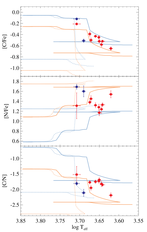
To investigate the influence of the extra-mixing process in our sample, we took advantage of models of Lagarde et al. (2012) where thermohaline convection and rotation-induced mixing are included. In parallel with our derived abundances, the model predictions for the stellar mass of 0.85 are shown in Fig. 6, considering the initial chemical compositions of [C/Fe] = , [N/Fe] = (blue lines) and [C/Fe] = , [N/Fe] = (orange lines), mimicking the primordial and enriched stellar populations, respectively. In term of carbon abundances, the observed data points are well constrained by models with [C/Fe] = — , and the abundance trend with follows exactly the model prediction. This implies that: a) the decrease in carbon abundance with decreasing is obviously a result of stellar evolutionary mixing; b) the initial carbon abundance spread among our sample stars is around 0.2 dex, which is slightly larger than our determination error ( 0.03 dex in average). On the other hand, the surface abundance of nitrogen is expected to increase as a result of extra-mixing, but the observed values do not follow the predictions of models with a single or a narrow range of initial [N/Fe]. Clearly, multiple models with initial [N/Fe] between +0.6 and +1.1 are needed to cover our data points. A difference of 0.5 dex in [N/Fe] is no doubt larger than the observed abundance errors ( 0.08 dex in average). Moreover, a scatter of about 0.7 dex in [C/N] can also be deduced, which is also significant compared with the error of 0.06 dex in average. Therefore, the existence of abundance variations among our observed member stars are suggested by (1) the apparent abundance distributions with no evolutionary effect considered (Fig. 4) and (2) the stellar evolutionary models considering extra-mixing processes of Lagarde et al. (2012) (Fig. 6). In conclusion, we find clear evidence that indicates the existence of MPs in GC Eridanus, particularly in nitrogen abundances.
4 Discussion
4.1 Eridanus
Given its higher metallicity ([Fe/H) compared to other outer halo GCs, and slightly younger age (10.5 Gyr), Eridanus is considered to have formed ex-situ. Carballo-Bello et al. (2015) speculated that Eridanus may be related to the Monoceros Ring since this GC lies in its predicted orbit. However, recent studies showed that the Monoceros Ring to be part of the outer Galactic disk with Galactocentric distances kpc (Li et al., 2021), and therefore their connection seems unlikely. On the other hand, Myeong et al. (2017) discovered two symmetrical tidal tails around Eridanus using g- and i-band deep imaging, which span about 760 pc in length. According to the great circle generated along the direction of the tidal tails, they instead suggested that Eridanus could have possible association with one of the four dwarf galaxies: Sculptor, Canes Venatici I, Canes Venatici II, and Fornax, of which Sculptor has a similar distance as Eridanus. The discovery of symmetrical, long tidal tails around Eridanus indicates that it has gone through a significant mass loss phase. This has two implications: 1. the initial mass should be much higher than the current mass, and thus our discovery of MPs in this GC does not necessarily contradict the current MP scenarios. A similar situation was found in Pal 13 (Tang et al., 2021); 2. Eridanus could have undergone stripping due to a radial orbit, causing stars to drift out from the Lagrange points of the cluster. However, its connection with low mass dwarf galaxies, e.g., Sculptor, may cause a logical dilemma. The existence of Eridanus is at odds with the lack of existing GC in Sculptor, and our discovery of N-enhanced stars in Eridanus is inconsistent with the null-detection of N-rich field stars in Sculptor (Lardo et al., 2016; Tang et al., 2022). Therefore, their association is less likely from a chemical point of view. Massari et al. (2019) analyzed the origins of Galactic clusters combining kinematic information and available cluster ages, where Eridanus is suggested to be accreted from a low-mass progenitor. There are still many unanswered questions regarding its origin, evolution, composition, and etc. The upcoming China Space Station Telescope (CSST) will give us a more complete picture of Eridanus by: 1. exploring its tidal tail mass with deep photometry; 2. investigating its cluster mass function and multiple populations on the main sequence with UV-optical filters.
4.2 Threshold mass for MP formation
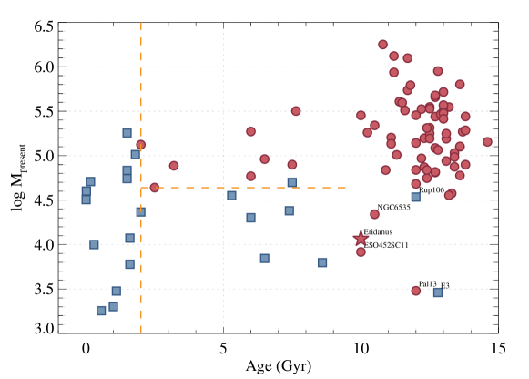
The distribution of age present-day mass for clusters with and without MPs was initially presented by Martocchia et al. (2018), where the data of the compilation by Krause et al. (2016) was considered. We further add data points from recent works, e.g., Salinas & Strader (2015); Niederhofer et al. (2017a, b); Simpson et al. (2017); Tang et al. (2017); Hollyhead et al. (2018); Zhang et al. (2018); Li & de Grijs (2019); Li et al. (2019, 2020); Milone et al. (2020); Tang et al. (2021); Fernández-Trincado et al. (2022), as well as this work (Fig. 7). We take the masses of the Milky Way GCs from the most recent version of the Galactic Globular Cluster Database from Baumgardt & Hilker (2018) which has been updated to include the Gaia EDR3 data. We also include data for several large clusters from the Large and Small Magellanic Clouds (LMC/SMC). The ages of the clusters have been taken from recent literature while their present-day masses are calculated by fitting N-body models to archival HST photometry, similar to what Baumgardt & Hilker (2018) have done for Galactic GCs. The initial masses for these clusters are calculated by using the present-day masses and applying the models of Baumgardt et al. (2013).
As previously suggested, the separation of clusters with and without MPs at the age of 2 Gyr can be clearly seen in the figure. For clusters younger than 10 Gyr, those with masses under 4.65 do not show MPs. However, the condition is ambiguous for GCs over 10 Gyr, since several low-mass GCs, e.g. NGC 6535 (Bragaglia et al., 2017), Eridanus (this work, represented by a red star), ESO452-SC11 (Simpson et al., 2017), Pal 13 (Tang et al., 2021), also possess MPs. According to the updated mass estimation, Pal 13 is the lowest-mass cluster with MP signals. The studies of old, low-mass GCs play a key role in revealing the MP formation and evolution.
During the long-time self evolution and co-evolution with MW, old GCs may experience complex mass loss. If a GC has an initial mass high enough to form MPs, and then loses a large amount of its mass during its long-time evolution, it can become an old, low-mass GC showing MPs. In this context, the information of cluster initial masses is fundamental to understand the MP formation (e.g., Carretta et al., 2010; Milone et al., 2020). Baumgardt et al. (2019) computed the initial masses for Galactic GCs using N-body simulation, while those of clusters in LMC/SMC will be presented in a forthcoming paper. In Fig. 8 we present the age-initial mass distribution of the cluster sample, where the LMC/SMC clusters without known initial masses are excluded. We find that the dispersion in initial cluster masses is smaller compared to that of their present-day masses, and most old (age 10 Gyr) GCs with MPs have initial masses above 5.2. Two of the aforementioned old low-mass GCs, NGC 6535 and ESO452-SC11, have initial masses as high as most of other old GCs, and thus their MPs can be easily explained. For Eridanus and Pal 13, considering their probable external origins, their real initial masses could be higher, since Baumgardt et al. (2019) only considered the GC orbits within the Milky Way in the simulation, and the mass loss before and during their merger into the Milky Way have been omitted.
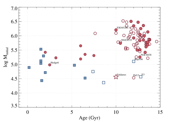
Considering uncertainties in the initial mass estimation for accreted clusters, in-situ ones can provide a simpler sample for analyzing the cluster mass threshold for MP formation. We divide the Galactic GCs into in-situ ones and accreted ones, according to category in Massari et al. (2019). Clusters in LMC and SMC are treated as in-situ ones (Fig. 8). In the in-situ sample, there is a slight trend in the clusters with MPs (older than 2 Gyr) that the older they are, the higher initial masses they have. Among them, NGC 6838 has the lowest initial mass of 5.26 at the old cluster end, while at the young cluster end, Hodge 6 has the lowest initial mass of 4.98. This may give a rough initial mass threshold, if it exists, for clusters to form MPs. However, more observations of old in-situ GCs with low initial masses, e.g., Pal 1 and Pal 11, are still necessary before drawing any firm conclusion.
5 Summary
Mass has been generally considered as one of the key parameters in deciding whether a stellar cluster will have MPs or not. In order to explore the possible mass threshold for MP formation, we studied the stellar population composition in low-mass GCs. In this work, we focus on the GC Eridanus, with a present-day mass of (Baumgardt et al., 2019).
Based on its CMD, we determined the age, metallicity, distance modulus and distance for Eridanus, which are 10.0 0.5 Gyr, -1.45 0.05 dex, 19.83 0.04 mag and 92.47 1.71 kpc, respectively. These are consistent with the values derived in previous studies.
In order to investigate whether MPs exist in Eridanus, blue-UV low-resolution spectra were obtained with OSIRIS/MOS on GTC for 19 member stars to study their carbon and nitrogen abundances. After determining their effective temperature and surface gravity photometrically, the spectral indices of CH4300 and CN4142 were computed for the final sample including nine RGB stars and two AGB stars. Then, with the help of model spectra, we derived the values of [C/Fe] and [N/Fe] for these stars. Since most of them have evolved past the RGB bump, where extra-mixing may significantly alter their surface chemical composition, we compared the observed abundances with stellar evolutionary models considering thermohaline instability and rotation-induced mixing. We find that besides the variations in carbon and nitrogen abundances caused by stellar evolution, the imprint of initial elemental abundance dispersion is prominently present in the observed nitrogen abundance distribution,which indicates the existence of MPs in Eridanus.
To find further investigate the critical cluster mass for MPs, we updated the age-mass distribution plane for all clusters having been studied for MPs. Although a threshold of present-day mass at 4.65 seems to exist for clusters younger than 10 Gyr, the condition for GCs older than 10 Gyr is unclear. Taking the mass loss during the long-time evolution of GCs into consideration, the initial mass of clusters should be a more reasonable parameter to analyze when studying the formation of MPs. We then constructed the age-initial mass plane with clusters in the Milky Way and LMC/SMC. To avoid the influence of the uncertainty in the initial mass estimation of accreted clusters, we simplified our sample with only in-situ clusters777We note that theoretically one does not expect the formation of MPs to depend on whether or not the cluster was formed in-situ or not.. Then, a slight trend that initial mass increases with increasing age is found for clusters (older than 2 Gyr) with MPs, and 4.98 and 5.26 are the lowest initial mass at the young and old end, respectively, which might provide a reference for the critical mass for clusters to form MPs.
However, the current observations are still incomplete for the study on this topic. Other low-initial-mass in-situ clusters are still necessary to be studied before we are able to have a comprehensive understanding. In this context, the up-coming space telescopes, e.g., the China Space Station Telescope (CSST) , as well as the ground based next-generation large telescopes, e.g., Thirty Meter Telescope and Extremely Large Telescope, will provide exciting opportunities for observations and studies in this field.
References
- Alonso et al. (1999) Alonso, A., Arribas, S., & Martínez-Roger, C. 1999, A&AS, 140, 261, doi: 10.1051/aas:1999521
- Armandroff & Da Costa (1991) Armandroff, T. E., & Da Costa, G. S. 1991, AJ, 101, 1329, doi: 10.1086/115769
- Asplund et al. (2005) Asplund, M., Grevesse, N., & Sauval, A. J. 2005, in Astronomical Society of the Pacific Conference Series, Vol. 336, Cosmic Abundances as Records of Stellar Evolution and Nucleosynthesis, ed. I. Barnes, Thomas G. & F. N. Bash, 25
- Bastian & Lardo (2018) Bastian, N., & Lardo, C. 2018, ARA&A, 56, 83, doi: 10.1146/annurev-astro-081817-051839
- Baumgardt & Hilker (2018) Baumgardt, H., & Hilker, M. 2018, MNRAS, 478, 1520, doi: 10.1093/mnras/sty1057
- Baumgardt et al. (2019) Baumgardt, H., Hilker, M., Sollima, A., & Bellini, A. 2019, MNRAS, 482, 5138, doi: 10.1093/mnras/sty2997
- Baumgardt et al. (2013) Baumgardt, H., Parmentier, G., Anders, P., & Grebel, E. K. 2013, MNRAS, 430, 676, doi: 10.1093/mnras/sts667
- Baumgardt et al. (2020) Baumgardt, H., Sollima, A., & Hilker, M. 2020, PASA, 37, e046, doi: 10.1017/pasa.2020.38
- Baumgardt & Vasiliev (2021) Baumgardt, H., & Vasiliev, E. 2021, MNRAS, 505, 5957, doi: 10.1093/mnras/stab1474
- Beccari et al. (2012) Beccari, G., Lützgendorf, N., Olczak, C., et al. 2012, ApJ, 754, 108, doi: 10.1088/0004-637X/754/2/108
- Bekki (2011) Bekki, K. 2011, MNRAS, 412, 2241, doi: 10.1111/j.1365-2966.2010.18047.x
- Blanco-Cuaresma (2019) Blanco-Cuaresma, S. 2019, MNRAS, 486, 2075, doi: 10.1093/mnras/stz549
- Blanco-Cuaresma et al. (2014) Blanco-Cuaresma, S., Soubiran, C., Heiter, U., & Jofré, P. 2014, A&A, 569, A111, doi: 10.1051/0004-6361/201423945
- Bragaglia et al. (2017) Bragaglia, A., Carretta, E., D’Orazi, V., et al. 2017, A&A, 607, A44, doi: 10.1051/0004-6361/201731526
- Carballo-Bello et al. (2015) Carballo-Bello, J. A., Muñoz, R. R., Carlin, J. L., et al. 2015, ApJ, 805, 51, doi: 10.1088/0004-637X/805/1/51
- Carretta et al. (2009) Carretta, E., Bragaglia, A., Gratton, R., D’Orazi, V., & Lucatello, S. 2009, A&A, 508, 695, doi: 10.1051/0004-6361/200913003
- Carretta et al. (2010) Carretta, E., Bragaglia, A., Gratton, R. G., et al. 2010, A&A, 516, A55, doi: 10.1051/0004-6361/200913451
- Cesarsky et al. (1977) Cesarsky, D. A., Laustsen, S., Lequeux, J., Schuster, H. E., & West, R. M. 1977, A&A, 61, L31
- Charbonnel & Zahn (2007) Charbonnel, C., & Zahn, J. P. 2007, A&A, 467, L15, doi: 10.1051/0004-6361:20077274
- Conroy & Spergel (2011) Conroy, C., & Spergel, D. N. 2011, ApJ, 726, 36, doi: 10.1088/0004-637X/726/1/36
- Da Costa (1985) Da Costa, G. S. 1985, ApJ, 291, 230, doi: 10.1086/163061
- de Mink et al. (2009) de Mink, S. E., Pols, O. R., Langer, N., & Izzard, R. G. 2009, A&A, 507, L1, doi: 10.1051/0004-6361/200913205
- Decressin et al. (2007a) Decressin, T., Charbonnel, C., & Meynet, G. 2007a, A&A, 475, 859, doi: 10.1051/0004-6361:20078425
- Decressin et al. (2007b) Decressin, T., Meynet, G., Charbonnel, C., Prantzos, N., & Ekström, S. 2007b, A&A, 464, 1029, doi: 10.1051/0004-6361:20066013
- Denissenkov & Hartwick (2014) Denissenkov, P. A., & Hartwick, F. D. A. 2014, MNRAS, 437, L21, doi: 10.1093/mnrasl/slt133
- Denissenkov et al. (2015) Denissenkov, P. A., VandenBerg, D. A., Hartwick, F. D. A., et al. 2015, MNRAS, 448, 3314, doi: 10.1093/mnras/stv211
- D’Ercole et al. (2010) D’Ercole, A., D’Antona, F., Ventura, P., Vesperini, E., & McMillan, S. L. W. 2010, MNRAS, 407, 854, doi: 10.1111/j.1365-2966.2010.16996.x
- Fernández-Trincado et al. (2022) Fernández-Trincado, J. G., Villanova, S., Geisler, D., et al. 2022, A&A, 658, A116, doi: 10.1051/0004-6361/202141742
- Gaia Collaboration et al. (2016) Gaia Collaboration, Prusti, T., de Bruijne, J. H. J., et al. 2016, A&A, 595, A1, doi: 10.1051/0004-6361/201629272
- Gaia Collaboration et al. (2018a) Gaia Collaboration, Brown, A. G. A., Vallenari, A., et al. 2018a, A&A, 616, A1, doi: 10.1051/0004-6361/201833051
- Gaia Collaboration et al. (2018b) —. 2018b, A&A, 616, A1, doi: 10.1051/0004-6361/201833051
- Gerber et al. (2020) Gerber, J. M., Friel, E. D., & Vesperini, E. 2020, AJ, 159, 50, doi: 10.3847/1538-3881/ab607e
- González Hernández & Bonifacio (2009) González Hernández, J. I., & Bonifacio, P. 2009, A&A, 497, 497, doi: 10.1051/0004-6361/200810904
- Gratton et al. (2004) Gratton, R., Sneden, C., & Carretta, E. 2004, ARA&A, 42, 385, doi: 10.1146/annurev.astro.42.053102.133945
- Gratton et al. (2000) Gratton, R. G., Sneden, C., Carretta, E., & Bragaglia, A. 2000, A&A, 354, 169
- Gustafsson et al. (2008) Gustafsson, B., Edvardsson, B., Eriksson, K., et al. 2008, A&A, 486, 951, doi: 10.1051/0004-6361:200809724
- Harbeck et al. (2003) Harbeck, D., Smith, G. H., & Grebel, E. K. 2003, AJ, 125, 197, doi: 10.1086/345570
- Harris (1996) Harris, W. E. 1996, AJ, 112, 1487, doi: 10.1086/118116
- Hollyhead et al. (2018) Hollyhead, K., Lardo, C., Kacharov, N., et al. 2018, MNRAS, 476, 114, doi: 10.1093/mnras/sty230
- Jester et al. (2005) Jester, S., Schneider, D. P., Richards, G. T., et al. 2005, AJ, 130, 873, doi: 10.1086/432466
- Krause et al. (2016) Krause, M. G. H., Charbonnel, C., Bastian, N., & Diehl, R. 2016, A&A, 587, A53, doi: 10.1051/0004-6361/201526685
- Lagarde et al. (2012) Lagarde, N., Decressin, T., Charbonnel, C., et al. 2012, A&A, 543, A108, doi: 10.1051/0004-6361/201118331
- Lardo et al. (2016) Lardo, C., Battaglia, G., Pancino, E., et al. 2016, A&A, 585, A70, doi: 10.1051/0004-6361/201527391
- Li & de Grijs (2019) Li, C., & de Grijs, R. 2019, ApJ, 876, 94, doi: 10.3847/1538-4357/ab153b
- Li et al. (2019) Li, C., Wang, Y., & Milone, A. P. 2019, ApJ, 884, 17, doi: 10.3847/1538-4357/ab3c54
- Li et al. (2020) Li, C., Wang, Y., Tang, B., et al. 2020, ApJ, 893, 17, doi: 10.3847/1538-4357/ab7b64
- Li et al. (2021) Li, J., Xue, X.-X., Liu, C., et al. 2021, ApJ, 910, 46, doi: 10.3847/1538-4357/abd9bf
- Martocchia et al. (2018) Martocchia, S., Cabrera-Ziri, I., Lardo, C., et al. 2018, MNRAS, 473, 2688, doi: 10.1093/mnras/stx2556
- Massari et al. (2019) Massari, D., Koppelman, H. H., & Helmi, A. 2019, A&A, 630, L4, doi: 10.1051/0004-6361/201936135
- Masseron et al. (2019) Masseron, T., García-Hernández, D. A., Mészáros, S., et al. 2019, A&A, 622, A191, doi: 10.1051/0004-6361/201834550
- McCall (2004) McCall, M. L. 2004, AJ, 128, 2144, doi: 10.1086/424933
- Mészáros et al. (2020) Mészáros, S., Masseron, T., García-Hernández, D. A., et al. 2020, MNRAS, 492, 1641, doi: 10.1093/mnras/stz3496
- Milone & Marino (2022) Milone, A. P., & Marino, A. F. 2022, Universe, 8, 359, doi: 10.3390/universe8070359
- Milone et al. (2017) Milone, A. P., Piotto, G., Renzini, A., et al. 2017, MNRAS, 464, 3636, doi: 10.1093/mnras/stw2531
- Milone et al. (2020) Milone, A. P., Marino, A. F., Da Costa, G. S., et al. 2020, MNRAS, 491, 515, doi: 10.1093/mnras/stz2999
- Muñoz et al. (2018) Muñoz, R. R., Côté, P., Santana, F. A., et al. 2018, ApJ, 860, 65, doi: 10.3847/1538-4357/aac168
- Mucciarelli & Bellazzini (2020) Mucciarelli, A., & Bellazzini, M. 2020, Research Notes of the American Astronomical Society, 4, 52, doi: 10.3847/2515-5172/ab8820
- Myeong et al. (2017) Myeong, G. C., Jerjen, H., Mackey, D., & Da Costa, G. S. 2017, ApJ, 840, L25, doi: 10.3847/2041-8213/aa6fb4
- Niederhofer et al. (2017a) Niederhofer, F., Bastian, N., Kozhurina-Platais, V., et al. 2017a, MNRAS, 464, 94, doi: 10.1093/mnras/stw2269
- Niederhofer et al. (2017b) —. 2017b, MNRAS, 465, 4159, doi: 10.1093/mnras/stw3084
- Osborn (1971) Osborn, W. 1971, The Observatory, 91, 223
- Pancino et al. (2010) Pancino, E., Rejkuba, M., Zoccali, M., & Carrera, R. 2010, A&A, 524, A44, doi: 10.1051/0004-6361/201014383
- Pancino et al. (2017) Pancino, E., Romano, D., Tang, B., et al. 2017, A&A, 601, A112, doi: 10.1051/0004-6361/201730474
- Piotto et al. (2012) Piotto, G., Milone, A. P., Anderson, J., et al. 2012, ApJ, 760, 39, doi: 10.1088/0004-637X/760/1/39
- Piotto et al. (2015) Piotto, G., Milone, A. P., Bedin, L. R., et al. 2015, AJ, 149, 91, doi: 10.1088/0004-6256/149/3/91
- Renzini et al. (2015) Renzini, A., D’Antona, F., Cassisi, S., et al. 2015, MNRAS, 454, 4197, doi: 10.1093/mnras/stv2268
- Salinas & Strader (2015) Salinas, R., & Strader, J. 2015, ApJ, 809, 169, doi: 10.1088/0004-637X/809/2/169
- Simpson et al. (2017) Simpson, J. D., De Silva, G., Martell, S. L., Navin, C. A., & Zucker, D. B. 2017, MNRAS, 472, 2856, doi: 10.1093/mnras/stx2174
- Stetson et al. (1999) Stetson, P. B., Bolte, M., Harris, W. E., et al. 1999, AJ, 117, 247, doi: 10.1086/300670
- Tang et al. (2022) Tang, B., Zhang, J., Yan, Z., et al. 2022, arXiv e-prints, arXiv:2210.06731. https://arxiv.org/abs/2210.06731
- Tang et al. (2017) Tang, B., Cohen, R. E., Geisler, D., et al. 2017, MNRAS, 465, 19, doi: 10.1093/mnras/stw2739
- Tang et al. (2021) Tang, B., Wang, Y., Huang, R., et al. 2021, ApJ, 908, 220, doi: 10.3847/1538-4357/abd557
- Vasiliev & Baumgardt (2021) Vasiliev, E., & Baumgardt, H. 2021, MNRAS, 505, 5978, doi: 10.1093/mnras/stab1475
- Ventura & D’Antona (2011) Ventura, P., & D’Antona, F. 2011, MNRAS, 410, 2760, doi: 10.1111/j.1365-2966.2010.17651.x
- Vesperini et al. (2010) Vesperini, E., McMillan, S. L. W., D’Antona, F., & D’Ercole, A. 2010, ApJ, 718, L112, doi: 10.1088/2041-8205/718/2/L112
- Wang et al. (2020) Wang, L., Kroupa, P., Takahashi, K., & Jerabkova, T. 2020, MNRAS, 491, 440, doi: 10.1093/mnras/stz3033
- Zhang et al. (2018) Zhang, H., de Grijs, R., Li, C., & Wu, X. 2018, ApJ, 853, 186, doi: 10.3847/1538-4357/aaa428