One-loop contributions to decays and anomalies, and Ward identity
Abstract
In this paper, we will present analytic formulas to express one-loop contributions to lepton flavor violating decays , which are also relevant to the anomalous dipole magnetic moments of charged leptons . These formulas were computed in the unitary gauge, using the well-known Passarino-Veltman notations. We also show that our results are consistent with those calculated previously in the ’t Hooft-Veltman gauge, or in the limit of zero lepton masses. At the one-loop level, we show that the appearance of fermion-scalar-vector type diagrams in the unitary gauge will violate the Ward Identity relating to an external photon. As a result, the validation of the Ward Identity guarantees that the photon always couples with two identical particles in an arbitrary triple coupling vertex containing a photon.
I Introduction
The lepton sector is one of the most interesting objects for experiments to search for new physics (NP) beyond the prediction of the standard model (SM). For example, the evidence of neutrino oscillation confirms that the SM must be extended. Recently, the experimental data of anomalous magnetic moments (AMM) of charged leptons has been updated, where the deviation between SM prediction and the lasted experiment data for muon is Muong-2:2021ojo
| (1) |
corresponding to the deviation from standard model (SM) prediction Aoyama:2020ynm combined from various contributions Davier:2010nc ; Davier:2017zfy ; Keshavarzi:2018mgv ; Colangelo:2018mtw ; Hoferichter:2019mqg ; Davier:2019can ; Keshavarzi:2019abf ; Kurz:2014wya ; Melnikov:2003xd ; Masjuan:2017tvw ; Colangelo:2017fiz ; Hoferichter:2018kwz ; Gerardin:2019vio ; Bijnens:2019ghy ; Colangelo:2019uex ; Colangelo:2014qya ; Blum:2019ugy ; Aoyama:2012wk ; Aoyama:2019ryr ; Czarnecki:2002nt ; Gnendiger:2013pva . For the electron anomaly, the deviation between SM and experiment is discrepancy Morel:2020dww .
On the other hand, are strongly constrained by the experimental data obtained from searching for the charged lepton flavor violating (cLFV) decays are MEG:2016leq ; BaBar:2009hkt :
| (2) |
This important property was discussed previously, for example see discussions for a general estimation in Ref. Crivellin:2018qmi , and many particular models beyond the standard model (BSM) Lindner:2016bgg ; Dorsner:2020aaz ; Hue:2021xap ; Hue:2021xzl ; Hong:2022xjg ; Li:2022zap . General formulas expressing simultaneously both one-loop contributions to AMM and cLFV amplitudes were introduced in the limits of new heavy scalar and/or gauge boson exchanges with being the mass of a charged lepton Crivellin:2018qmi . Other calculations in the unitary gauge were discussed Yu:2021suw ; Leveille:1977rc for the one-loop contributions to with , without the relations with the cLFV amplitudes. The analytic one-loop formulas for cLFV amplitudes calculated in the ’t Hooft Feynman (HF) gauge were also shown in Ref. Lavoura:2003xp , using the notations of the Passarino-Veltman (PV) functions Passarino:1978jh ; tHooft:1978jhc with . The approximate formulas with were introduced and consistent with those given in Ref. Crivellin:2018qmi , as shown particularly in Ref. Hue:2017lak for 3-3-1 models. The general analytic formulas of these PV functions were introduced for numerical investigations. They are consistent with the results generated by LoopTools Hahn:1998yk , which can be transformed into other PV notations implemented in the Fortran numerical package Collier Denner:2016kdg , used to investigate cLFV decays in a two Higgs doublet model (2HDM) Jurciukonis:2021izn . Many particular expressions to compute the AMM and/or cLFV decay amplitudes predicted by different particular BSM were constructed Lindner:2016bgg . The relations among them can be checked by using suitable transformations, starting from the set of particular PV notations in this work. On the other hand, in a discussion on analytic formulas for one-loop contributions to AMM, a class of fermion-scalar-vector () diagrams consisting of a photon coupling with two different physical particles, namely one scalar and one gauge boson, were considered even in the unitary gauge Yu:2021suw . It leads us to whether the Ward identity (WI) for the external photon is still valid with the presence of this diagram type. We emphasize that the general results for one-loop contributions to decays and AMM of leptons introduced in many previous works do not include these diagrams. Moreover, they imply the existence of the triple photon coupling with two distinguishable physical particles that has never been mentioned previously. In particular, many works introducing general one-loop contributions for AMM of charged leptons Leveille:1977rc ; Lindner:2016bgg ; Crivellin:2018qmi , or decays relating with photon such as cLFV decays Lavoura:2003xp ; Lindner:2016bgg ; Crivellin:2018qmi , loop-induced Higgs decays Gunion:1989we ; Bunk:2013uea , Bunk:2013uea ; Hue:2017cph ; Phan:2021xwc ; VanOn:2021myp , quark decays , . Excluding the vertex type will reduce a huge number of related one- and two-loop diagrams as well as confirm the validation of general one-loop calculation introduced previously.
In this work, we will show precisely the important steps to derive the one-loop contributions to both AMM and cLFV decays. The calculation is performed by hand, which is consistent with another cross-checking using FORM package Vermaseren:2000nd . The final formulas are expressed exactly in terms of the PV functions defined by LoopTools. The results are then easy to change into all the other available forms using suitable transformations. The conventions of the PV-functions are very convenient to derive the exact formulas before solving particular pure mathematical problems. We also determine contributions arising from a new form of photon coupling with vector bosons such as leptoquarks and confirm the consistency between our results and those introduced in Ref. Bunk:2013uea ; Barbieri:2015yvd ; Biggio:2016wyy .
Our paper is organized as follows. Section I explains our aim of this work. Section II introduces notations and important formulas to establish the relations between AMM and cLFV amplitudes. Section III shows discussions to confirm the consistency of our results and previous works, and the validation of the WI for the relevant analytic formulas. Section IV summarizes main features of our work. Finally, we provide many appendices showing precisely many intermediate steps and notations to derive the final results mentioned in this work, including the analytic formulas of the PV functions consistent with LoopTools given in appendix A.
II General amplitudes and notations
It is well-known that analytic formulas of one-loop contributions to the cLFV amplitudes and AMM of SM charged leptons can be presented in the same expressions, see for example Ref. Crivellin:2018qmi corresponding to the presence of new heavy particles in BSM. Possible one-loop Feynman diagrams contributing to and cLFV decay amplitudes in BSM are shown in Fig. 1, where is a fermion coupling with the SM charged lepton ; and the boson is a scalar or gauge boson, respectively.
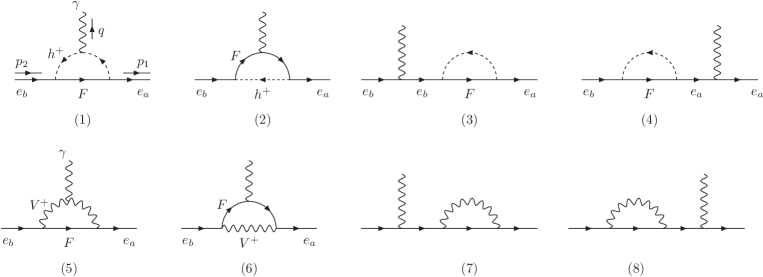
For a detailed calculation, precise conventions for external momenta and propagators are presented in appendix C. We note here that Ref. Yu:2021suw argues another type of one-loop diagrams giving new contributions to the AMM. They will be discussed in detail in this work.
Firstly, we adopt the Lagrangian generating one-loop diagrams in Fig. 1, namely Crivellin:2018qmi
| (3) | ||||
| (4) |
where the fermion and the boson have electric charges and , and masses and , respectively. These Lagrangians (3) and (4) are consistent with those in Ref. Lavoura:2003xp . Moreover, the photon couplings with all physical particles should be mentioned clearly, as given in Ref. Lavoura:2003xp , i.e., we will adopt the Feynman rules that the photon always couples with two identical physical particles, as given in table 1,
| Vertex | Coupling | Vertex | Couplings | Vertex | Couplings |
|---|---|---|---|---|---|
where is the standard form. The more general form of introduced in Refs. Bunk:2013uea ; Barbieri:2015yvd ; Biggio:2016wyy will be discussed in detail later.
All couplings listed in Lagrangians (3), (4), and table 1 result in the following form factors relevant with one-loop contributions:
| (5) |
where . The four scalar functions , , , and are listed in Eq. (58) of appendix A, as the approximate formulas in the limit . The formula in Eq. (II) does not contain contributions from the diagrams mentioned in Ref. Yu:2021suw , because of the absence of photon coupling . The corresponding formulas of AMM and cLFV decay rates are:
| (6) | ||||
| (7) |
where , , and are the masses and total decay width of the leptons , , and
| (8) |
The amplitude for a vertex in Ref. Peskin:1995ev is consistent with the following form presenting both AMM and cLFV amplitudes Escribano:1996wp ; Eidelman:2016aih
| (9) |
where ; are scalar form factors; and is the polarized vector of the external photon. The derivation of Eq. (9) respecting the WI from the most general form was explained clearly in Ref. Eidelman:2016aih . The form factors get contributions only from loop corrections. They relate with the well-known experimental quantities called the anomalous magnetic moment and electric dipole moment for , respectively. Specifically, we have for the on-shell photon, and
| (10) |
Regarding the LFV decay the amplitude can also be written in the same form Cheng:1984vwu ; Lavoura:2003xp , suggesting that can be calculated based on the one-loop corrections to LFV decays. In particular, the second term of the amplitude (9) can be expanded as follows Hue:2017lak
| (11) |
where and we can prove that . The WI for the external photon gives
| (12) |
We note that although WI does not require the condition of on-shell photon in general, it was also used to derive the two relations given in Eq. (12), which simplify our calculation in the unitary gauge 222We thank the referee for reminding us this point. The general case of is beyond our scope, see Ref. Jurciukonis:2021izn for a detailed discussion of this case in the 2HDM framework. The hermiticity that Eidelman:2016aih gives
| (13) |
Hence, the following relations between two different notations must be satisfied:
| (14) |
From the above discussion, we see that one-loop contributions to the and can be written in terms of well-known PV functions, see detailed discussions in Ref. Hue:2017lak or general formula introduced for calculations of the cLFV decay rates Lavoura:2003xp , with the identification that . In the limit of , the numerical values of can be evaluated using the numerical packages such as LoopTools Hahn:1998yk or Collier Denner:2016kdg . Although the exact analytic formulas of one-loop three-point functions presented in Ref. Hue:2017lak can not be applied to calculate , the limit of can be used to solve this problem. The analytic formulas of were introduced completely in Ref. Yu:2021suw .
Because of the relations in Eq. (12), only is needed to determine and Br. Because all two-point diagrams give contributions to just , are calculated by considering only three-point diagrams. In this work, the analytic formulas of will be determined directly from all diagrams in Fig. 1 to check the validation of the WI in the presence of the .
The analytic formulas for one-loop contributions to the cLFV decay amplitudes presented in this work are more general than the results introduced in Ref. Hue:2017lak for general 3-3-1 models. Many important steps in our calculations were shown in appendix C. Using this unitary gauge, the assumption for a particular form of the Goldstone boson couplings given in Ref. Lavoura:2003xp is unnecessary. In contrast, we use the same photon couplings to other physical particles in an arbitrary BSM, as given in table 1. Namely, a tree-level photon coupling always contains two identical physical particles. This implies that the contributions from the diagrams are not included.
Using the notations of PV-functions defined in appendix A, the contributions from diagram (1) in Fig. 1 are:
| (15) |
where are linear combinations of the PV-functions defined precisely in appendix A.
The diagram (2) in Fig. 1 gives contributions as follows:
| (16) |
where are linear combinations of . The above results are completely consistent with those introduced in Ref. Lavoura:2003xp , except an overall sign and the signs before the PV-functions , arising from the different definitions of the external momenta in the denominators of the one-loop integrals. We also give the analytic formulas of and , used to confirm the WI given in Eq. (12) for the only-scalar contributions. The PV-functions derived from diagram (2) defined as are different from defined for three diagrams (1), (3), and (4). In contrast, the equal functions are denoted as follows:
The form factors originated from scalar contributions are:
| (17) |
where are linear combinations of , , and given in Eq. (37).
It is noted that the contributions are the sum of three diagrams (1), (3), and (4), while the contributions are from only diagram (2). We emphasize that the electric charge conservation is one of the necessary requirements to guarantee the WI given in Eq. (12), see a detailed proof in appendix C. We can see this crudely from the necessary condition that div and div. This conclusion supports completely the only case of electric conservation among the remaining ones mentioned in Ref. Lavoura:2003xp .
Regarding Lagrangian (4), which results in four diagrams in the second line of Fig. 1, diagram (5) gives the following contributions:
| (18) |
where is the linear combinations of , given in Eq. (40), and
| (19) |
Diagram (6) gives contributions:
| (20) |
where all are expressed in terms of PV functions , and
| (21) |
Finally, using the simple notations , the formulas of and are
| (22) | ||||
| (23) |
where all are expressed in terms of PV functions and is given in Eq. (37).
The remaining formulas of from diagram (6) of Fig. 1 are
| (24) |
where all are expressed in terms of PV functions and is given in Eq. (37).
We note that all results presented here are crosschecked by FORM package Vermaseren:2000nd , using intermediate steps given in appendix C. There is a property that for all . The above results of one-loop contribution to are totally consistent with those introduced in Ref. Lavoura:2003xp , after some transformations of notations presented in appendix B. In the limit of , i.e., with , we get consistent results with those given in Ref. Crivellin:2018qmi ; Freitas:2014pua ; Stockinger:2006zn . To derive the above results for gauge boson exchanges, we start with many important features different from those mentioned in Ref. Lavoura:2003xp , namely: i) we do not use the typical form of couplings relating to Goldstone bosons going along with the presence of new gauge bosons, ii) we have to use the massless property of the on-shell photon , iii) to confirm the WI for all diagrams given in Fig. 1, we need the charge conservation law corresponding to the Lagrangian (1): . Therefore, our calculation is another independent approach to confirm the result given in Ref. Lavoura:2003xp . The details of the calculation to confirm the WI for all one-loop contributions are given in appendix C. We remind that our results are derived from the photon couplings listed in the table 1, and do not contain the contributions from the FSV diagrams. In the following, we pay attention to the possibility of adding the FSV diagrams or the new forms of the photon couplings.
III Discussion on WI and previous results
III.1 WI to constrain the form of photon couplings
Now we focus on the feature that the WI of the on-shell photon will constrain strongly the forms of the cubic photon couplings with two physical particles in a renormalized Lagrangian. Now we consider the existence of the photon coupling types at tree level:
| (25) |
where all couplings are more general than those well-known as the standard forms given in Table 1. In addition, the last term corresponds to the photon coupling to a scalar and a gauge boson mentioned in Eq. (110). The above Lagrangian results in the following decays from the heavy particle to the lighter one: i) , ii) , iii) , and iv) . The WI for these decay amplitudes at tree level is with being the external photon momentum. It can be derived that:
-
•
Using the same convention of external momenta given in Fig. 1, we have , where . Therefore, . This case is automatically satisfied for the tree-level AMM amplitude.
-
•
, where all on-shell momenta are incoming the vertex , implying that and . The consequence is .
-
•
, where and are the polarization of gauge boson and the external momentum of the photon . Hence, the presence of a vertex does not automatically satisfy the WI. One-loop contributions for all diagrams arising from this vertex must be checked for the validation of WI. In Ref. Yu:2021suw , the presence of these vertices was mentioned in a Higgs triplet model (HTM). A detailed calculation in appendix E shows an opposite conclusion that this vertex vanishes at tree level 333To the best of our knowledge, we have not seen any UV models beyond the SM that have violated couplings of the form --, which is the necessary source for generating -type diagrams..
-
•
, where , and are the polarization of the gauge boson and the external momentum of the gauge bosons and photon , respectively. We will use the following properties of the external gauge bosons and photon: , , , and the momentum conservation following notations in table 1. After some intermediate calculating steps, we have:
(26) Hence, is necessary. From this, we consider the more general photon coupling with a gauge boson Biggio:2016wyy describing the couplings of a leptoquark field Barbieri:2015yvd
(27) with showing the deviation from the standard vertex listed in table 1. This may change the one-loop contributions of the diagram (5) in Fig. 1, hence change the formulas of given in Eqs. (II) and (II), respectively. One can prove immediately that the vertex deviation
(28) guarantees the WI. The new one-loop contributions arising from are also satisfied the WI, see analytic formulas given in Eq. (C.2).
Now we start from the point that all results of one loop contributions given from Eq. (II) to Eq. (II) based on the standard forms of photon couplings given in table 1, where a photon always couples with two identical physical fields. On the other hand, a recent work Yu:2021suw assumed the existence of a new photon coupling kind , which may appear in some BSM, in which the photon couples with one gauge boson and one scalar . The appearance of a boson or will generate by itself the one-loop contributions that always guarantee the WI by the respective set of four diagrams given in Fig. 1. Hence, the two FSV diagrams must give contributions satisfying the WI themselves, namely
| (29) |
As a result, the divergent parts of given in appendix D for both and parts give:
| (30) |
Considering the case of . Then, all quantities , , and are zeros if at least one of them is zero. More strictly, we require that the two Eqs. (29) must be held for both divergent and finite parts arising from and given in appendix D. Consequently, , i.e., the diagram type does not satisfy the WI.
Regarding the vertex deviation of the couplings defined in Eq. (28), the new one-loop contributions relating to and are shown in Eq. (C.2) of appendix C. Our results are consistent with previous works Barbieri:2015yvd ; Biggio:2016wyy . Although they satisfy the WI, they contain divergences. For example, the divergent part of is
| (31) |
Hence, is equivalent to the renormalizable condition of the theory, see a more detailed explanation in Ref. Biggio:2016wyy . This confirms that the coupling listed in table 1 is still valid for a general UV-complete model. Consequently, , implying that the results of given in Eqs. (II) and (II) are unchanged for many renormalizable theories.
III.2 Discussions on previous results
It is easy to derive that corresponding to the notations given in Ref. Lavoura:2003xp , see a detailed explanation in appendix B. This confirms a perfect consistency of the two results obtained from different original assumptions that we have indicated above. In addition, these results are also consistent with those given in Ref. Crivellin:2018qmi in the limit of heavy boson masses in the loops, which are very useful for studying the correlations of AMM and cLFV decays.
In some BSM, SM light quark may play the role of the light fermions in the Yukawa couplings Dorsner:2020aaz , hence the condition is not held. But numerical illustrations Hue:2017lak to investigate cLFV decays with very light neutrinos show that the case of is also valid for approximation formulas with , provided . An analytic approximation to explain this result was given in, for example, Ref. Hue:2015fbb .
For analytic formulas of cLFV and introduced in Ref. Lindner:2016bgg , They can be changed into the form of PV-functions consistent with our results. An exceptional case mentioned is the coupling of a doubly charged boson with two identical leptons. For example, the Lagrangian containing couplings of a doubly charged Higgs boson is Lindner:2016bgg :
| (32) |
where we can identify that and . But the Feynman rules for the vertex containing two identical leptons give an extra factor 2, implying that given in Eqs. (II) and (II) must be added a factor 4. Instead of many particular formulas to calculate one-loop contributions relating to different charged particles, the one-loop results for and decays can be generalized for with an arbitrary electric charge of a new fermion and the boson with with . Namely, the formulas are
| (33) | ||||
| (34) |
where , , and with . The coupling identifications are and for relating to neutral, singly, and doubly charged Higgs bosons. Similarly to the gauge bosons, and for corresponding . The two formulas (33) and (34) are derived by inserting the PV functions given in appendix A in the limit into . We have checked that our results are consistent with all , , and contributions relating to the diagrams (1), (2), and (6) in Fig. 1, respectively. For the one-loop contributions arising from the diagram (5), there is a difference between our result and that in Ref. Lindner:2016bgg , namely
It shows that the two results are consistent if ,i.e., , which appears in many BSM such as the SM, 3-3-1 models,… We also see that the contribution to of the doubly gauge boson given in Ref. Lindner:2016bgg has an opposite sign with our result.
We note that our results are also valid as the exact solutions for studying the AMM and decay in BSM consisting of very light bosons such as an axion-like particle (ALP) Bauer:2019gfk ; Cornella:2019uxs , or a new scalar singlet Liu:2018xkx .
IV Conclusion
Using the unitary gauge, we confirm the exact results of analytic formulas in terms of PV functions for one-loop contributions to the cLFV decay rates given in Ref. Lavoura:2003xp , which are also applicable to compute the AMM of charged leptons. These results are consistent with those given in Ref. Crivellin:2018qmi in the limit of heavy bosons . The general expressions in terms of PV-functions are very convenient to change into available forms. Our calculations here have many new features as follows. Our calculation is independent of the Goldstone boson couplings of the new gauge bosons. The Ward Identity of the external photon allows only the couplings of a photon with two identical physical particles, as given in table 1. At tree-level, the couplings do not satisfy the WI if , where and are the polarization of gauge boson and the external momentum of the photon, respectively. The one-loop contributions arising from this vertex type to cLFV amplitudes and AMM do violate the WI. Therefore, the results given in Ref. Lavoura:2003xp ; Crivellin:2018qmi are valid in all renormalizable BSM respecting the WI. They are still applied for other similar decays of quarks . The photon-scalar-vector vertex does not appear in BSM satisfying the WI. Our conclusion is very useful for constructing loop calculations relating to photon couplings, where only the vertex types listed in Table 1 are valid.
Acknowledgments
The authors thank the referee for suggesting an open question about the existence of the -- couplings in the UV models, which we will solve more generally in our future work. This research is funded by the Vietnam National Foundation for Science and Technology Development (NAFOSTED) under the grant number 103.01-2019.387.
Appendix A PV functions for one loop contributions defined by LoopTools
A.1 General notations
The PV-functions used here were listed in Ref. Hue:2017lak , namely
| (35) |
where , , , is an arbitrary mass parameter introduced via dimensional regularization tHooft:1972tcz . In this work, we discuss only the case of external photon . The scalar functions , and () are well-known PV functions, which are consistent with those defined by LoopTools Hahn:1998yk . The well-known relations are:
| (36) |
where . Depending on the particle exchanges in Feynman diagrams, the -function given in Eq. (A.1) is denoted more precisely as follows:
| (37) |
The scalar functions , , and can be calculated using the techniques of tHooft:1978jhc . Other PV functions needed in this work are
| (38) |
For simplicity, we define the following notations appearing in many important formulas:
| (39) |
Depending on the form of the PV-functions, we have
| (40) |
corresponding to the diagram types of , , and with .
A.2 and .
From the definitions of PV-functions given in Eq. (35), it can be proved that:
| (41) | |||
| (42) | |||
| (43) |
where is defined as the divergent part of the PV functions when , with being Euler’s constant and . It is well-known that the PV-functions having non-zero divergent parts are:
| (44) |
As mentioned in Ref. Hue:2017lak , we can derive all formulas of , and as functions of , , and consistent with Ref. Hue:2017lak , using the following relations:
| (45) |
where , and are used. In this work, we need just combinations of these PV-functions for our immediate steps. In particular, we can prove that:
| (46) |
where and .
It was proved previously, for example Hue:2017lak , that
| (47) |
where ; and
| (48) |
with . The above formula of is also consistent with that introduced in loop-induced decay amplitude of Djouadi:1996yq .
A.3
Formulas for AMM in Ref. Yu:2021suw require that analytic formulas of PV functions with . It seems that the results of PV-functions listed in Ref. Hue:2017lak are not valid. But the limit can be derived mathematically. For example, the result of given in Eq. (A.2) leads to a consequence that
| (49) |
where denotes a well-known derivative notation. In addition, and are automatically satisfied. Many formulas containing in the denominators corresponding a derivative in the limit :
| (50) |
In this way, we can confirm all results introduced in Ref. Yu:2021suw . There is another way to calculate form factors, using the Feynman trick:
| (51) |
where
| (52) |
With , the PV functions are:
| (53) |
The expressions of in Eq. (A.3) are very convenient for the case of anomaly, where results in , which is independent with . Consequently, the
| (54) |
Formulas of Eq. (A.3) are enough to check the consistency between our results with those of anomalies and cLFV amplitudes mentioned in ref. Lindner:2016bgg . Using the second line of Eq. (A.3), we can write the general formulas of as shown in Eqs. (33) and (34).
Indeed, all integrals in Eqs. (33) and (34) can be solved analytically. Starting from the general formulas of as functions of : corresponding to the two solutions . All numerators in Eqs. (33) and (34) are always written in the following forms:
| (55) |
The consequence is
| (56) |
The result in this way must be consistent with those discussed in Ref. Yu:2021suw , hence we do not show precisely here.
A.4
Results for the case of were provided in Ref. Lavoura:2003xp , namely
| (57) |
This approximate formulas of PV functions give results consistent with those given in Ref. Crivellin:2018qmi , namely
| (58) | |||
where . The diagrams and correspond to different identifications that or and .
Appendix B Notations in Ref. Lavoura:2003xp
Here we give a brief review of the approach of Ref. Lavoura:2003xp . Apart from the general couplings of physical Higgs and gauge bosons given in Eqs. (3) and (4), the photon couplings were assumed to be the standard forms given in table 1. Furthermore, the couplings of the Goldstone boson corresponding to are assumed to be the following forms:
| (59) |
The above assumptions of the couplings are necessary for the calculation of one-loop gauge contributions that were done in the ’t Hoof Feynman gauge. These final results introduced in Ref. Lavoura:2003xp were the sum of all diagrams consisting of gauge and Goldstone boson exchanges. Corresponding to the two one-loop diagram classes and , we have the following equivalence between two classes of notations
where are gauge bosons in the loop. In addition, the different notations in the definitions of the one-loop integrals given in Eq. (35), we have while and for the diagrams and respectively. The couplings in the Yukawa Lagrangian of physical bosons are , , , and , which result in the following equivalences: , , , and . As a result, we can identify that:
| (60) |
For a gauge boson , the one-loop form factors relate to the following notations:
| (61) |
and
| (62) |
Appendix C Important steps to derive and by hand
The notations for calculating the amplitude corresponding to all diagrams of both Higgs and gauge boson exchanges in Fig. 1 are shown in Fig. 2.
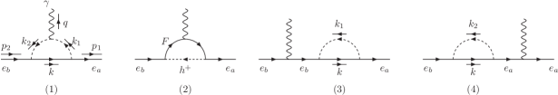
All diagrams in the same class will have the same conventions of external momenta and propagators. There are three classes of diagrams: i) The first class consists of four diagrams (1), (2), (5), and (6) in Fig. 1, and the two diagrams (1) and (2) in Fig. 2; ii) the second class consists of three diagrams: (3) and (7) in Fig. 1, and (3) in Fig. 2; iii) the last class consists of the remaining diagrams in the two Figs. 1 and 2. Although all the internal momenta have opposite signs with those denoted following LoopTools, the PV-functions are defined with the same values. The relations relevant to momenta are:
| (63) |
Only four diagrams (1), (2), (5), and (6) in Fig. 1 give non-zero contributions to , hence we firstly derive as the factors of in the amplitudes arising from these diagrams. For convenience in detailed calculations, we use simple notations for all the coupling factors . For integrals containing divergences, we use the regular dimensional regularization defined by the following replacement:
The final results now are written in terms of the PV functions. In many intermediate steps, we use many results for products of gamma matrices in the dimension Peskin:1995ev , namely
C.1 Scalar contributions
We list here 8 formulas of amplitudes corresponding to 8 particular diagrams shown in Fig. 1. Namely, for three diagrams (1), (3), and (4) we have
| (64) | ||||
| (65) | ||||
| (66) |
where and . The amplitude for the diagram (2) is:
| (67) |
where and .
In the next calculation, we use the following simple notations:
| (68) |
where and without any confusions with the gauge boson couplings . It is not hard to write all amplitudes in terms of PV-functions as follows:
| (69) | ||||
| (70) | ||||
| (71) |
and
| (72) |
The validation of the WI given in Eq. (12) implies whether is correct with:
| (73) |
We have used many formulas listed in Eqs. (A.1) and (A.2) to show that
| (74) |
Finally, the electric charge conservation must be satisfied so that Eq. (C.1) resulting in . On the other word, the WI is valid for only one-loop Higgs contributions arising from the set of four diagrams (1)-(4) in Fig. 1.
C.2 Vector contributions
To calculate the one-loop contributions from gauge boson exchanges corresponding to Lagrangian (4), we denote and then use the notations given in Eq. (C.1). The amplitudes relevant with gauge boson exchanges are:
| (75) | ||||
| (76) | ||||
| (77) |
where , , and
| (78) |
The amplitude for the diagram (6) is:
| (79) |
where and .
Considering diagram (7), we have:
| (80) |
where we have used the following results
Then the one-loop contribution form factors from diagram (7) are:
| (81) |
The same calculation for diagram (8) gives the following one-loop contribution form factor:
| (82) |
Using and the divergent parts of PV-functions given in Eq. (A.2), we get the formulas of given in Eq. (22).
Diagram (5)
From the equalities , , and , it is easy to prove that
| (83) |
As a result, the amplitude (75) is written as follows:
| (84) |
where
| (85) |
The first term in the integrand is
| (86) |
After integrating out, the formula is
| (87) |
The second term in the integrand is
| (88) |
The first term in Eq. (C.2) gives
| (89) |
Because the divergent part , which , hence . The result is:
| (90) |
where we have used and . The final result is
| (91) |
Consider the last two terms in the last line of the formula (C.2)
| (92) |
Lastly, consider the first term in the last line of the formula (C.2):
| (93) |
where and . The last line in Eq. (C.2) is expressed in terms of the PV functions as follows
| (94) |
Hence the final result of Eq. (C.2) is
| (95) |
The sum of three terms given in Eqs. (C.2), (C.2), and (C.2) gives corresponding to the diagrams (5) given in Eqs. (II) and (II). The formulas of and are given in Eq. (23).
Regarding to the case of photon couplings in Eq. (• ‣ III.1), the equality given in Eq. (C.2) is still valid because the new part satisfies . The other relevant part of is:
| (96) |
The final result of new contributions to is:
| (97) |
Ignoring the factor , the form factors are:
| (98) |
All results given in Eq. (C.2) were cross checked using FORM package Vermaseren:2000nd . All formulas in Eq. (C.2) satisfy automatically the WI, namely .
Diagram (6)
After using the property of chiral operators , the amplitude (C.2) is written as
| (99) |
The numerator is divided into the two parts and . After extracting , the first part is
| (100) |
Ignoring the overall factor , the formula in terms of tensor notations is
| (101) |
After expanding the tensors in terms of scalar PV-functions, the final result is
| (102) |
Considering the second term proportional to , we have
| (103) |
The two relations and give
| (104) |
where
It can be proved that:
| (105) |
Final results are:
| (106) |
The above calculation is enough to derive relevant contributions to given in Eqs. (II) and (II), and given in (II).
Ward identity for the only gauge boson exchanges
Before coming to discuss the WI, we use the relations given in Eq. (A.2) to write all the one-loop factors (22), (23), and (II) from gauge boson exchanges in the following simple forms, ignoring the overall factor :
| (107) |
The WI for the and diagrams are and , respectively. The relations given in Eq. (A.2) give:
| (108) |
Combining the above formulas and results of functions listed in Ref. Hue:2017lak , the WI of all diagrams with boson exchanges is derived as follows
| (109) |
The final result is . In conclusion, the contributions from the four diagrams with only gauge boson exchanges satisfy the WI when the electric charge conservation is valid.
Appendix D Ward Identity for the diagrams of FSV-type in the unitary gauge
This type of diagrams were mentioned firstly in Ref. Yu:2021suw for the general case of their contributions to BSM. The vertices come the kinetic terms of the scalars:
| (110) |
where containing the photon and is the covariant part of the covariant derivative of the Higgs multiplets. The Feynman diagrams in the general gauge are shown in Fig. 3.
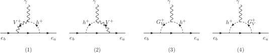
Here only two diagrams (1) and (2) give non-zeros contributions in the unitary gauge, which correspond to the two diagrams (b) and (a) in Fig. 5 introduced in Ref. Yu:2021suw . In this gauge, the contributions of these two diagrams are:
| (111) |
where we have used . The formulas of and are:
| (112) |
where . Similarly, the results for diagram (10) are:
| (113) |
where . The above formulas are consistent with calculation using FORM. The corresponding formulas of WI are
| (114) |
where . The WI is valid if only . We can see crudely that all , , , and are convergent. In contrast, all , , , and contain divergent terms. Therefore, the necessary condition to guarantee the validation of the WI given in Eq. (12) is that all of these divergent terms must vanish. Strictly, the WI is valid if only =0 or . Because at least one of or must be non-zero, the condition =0 is the only valid choice, i.e., the vertex-type -- does not appear in the all BSM guaranteeing the WI for the external photon. This conclusion is also true for the case , corresponding to the one-loop contribution to the AMM of the leptons.
Finally, using the assumption of the Lagrangian for couplings of the Goldstone boson given in Eq. (B), we can determine the one-loop contributions of the FSV diagrams mentioned above, using the general gauge . The propagator of the gauge boson can be written in terms of two separated parts:
| (115) |
where is the propagator in the unitary gauge, and relates to the propagator of as follows:
| (118) |
For two diagrams (3) and (4) in Fig. 3, the Feynman rules for the couplings are the same form as those given in Lagrangian (III.1), namely and . The reason is that all mass eigenstates of the scalar with the same electric charges come from the same squared mass matrix. Therefore, . Formulas corresponding to diagrams (1) and (3) of Fig. 3 in the general gauge are
where , , , and is exactly the part given in Eq. (D), calculated in the unitary gauge. The results of the two diagrams (1) and (3) are:
| (119) | ||||
| (120) |
where and .
As we showed clearly in Eq. (115), a propagator of an arbitrary internal gauge boson always consists of two parts: i) the first part is exactly the unitary propagator resulting in , and ii) the second is proportional to the propagator of the respective Goldstone boson, in which the parameter defines a new mass value in the denominator, which results in . Because is arbitrary, the two one-loop contributions corresponding to the two mentioned parts are independent. As a result, the WI violation of the contributions relating to is enough to guarantee that the contributions from the FSV-type diagrams always violate the WI.
Appendix E Higgs gauge couplings in the Higgs triplet models
Here we summarize the HTM and derive precisely the Higgs gauge couplings. The Higgs sector consists of a Higgs triplet and a Higgs doublet in the electroweak gauge symmetry corresponding to the electric operator . Here we will use the notations from Ref. Ashanujjaman:2021txz ; Aoki:2011pz , the Higgs sector is
| (121) |
where and are the vacuum expectation values (VEV) of the neutral Higgs components. Because has the lepton number 2, .
The Higgs gauge couplings appear in the following kinetic terms:
| (122) |
where
| (123) |
The masses and mixing parameters of the gauge bosons are derived from the Eq. (122), with VEVs of and . A detailed calculation shows that the physical states , neutral and photon are:
| (124) |
The respective masses are , and the photon is massless. The relation is well-known, the same as that in the SM. The covariant derivatives in Eq. (123) are written in the mass eigenstates as follows:
| (125) |
where we just focus on the couplings relating to the vertex . Therefore, the relevant parts in the kinetic term are:
| (126) |
The Higgs potential of all Higgs multiplets was investigated previously, for example, Ashanujjaman:2021txz ; Aoki:2011pz . The results of masses and mixing parameters of all Higgs bosons are confirmed by our careful cross-check. We focus on the Higgs gauge couplings of the singly charged Higgs boson in this model, the mixing parameter relating to mass eigenstates and the original ones are:
| (127) |
Here is the Goldstone bosons of , while is the only singly charged Higgs boson predicted by the HTM. Then the couplings , and the couplings with are , consistent with the SM. In contrast, Ref. Yu:2021suw seems to take into account only the contribution of to , and ignored that of , although they have the same amplitude but opposite signs.
It is noted that the results derived from our calculation are consistent with those in recent works discussing all tree-level decays of Higgs and gauge bosons predicted by the HTM at LHC Ashanujjaman:2021txz ; Aoki:2011pz . The decays do not appear in the decay lists of these works.
References
- (1) B. Abi et al. [Muon g-2], Phys. Rev. Lett. 126, no.14, 141801 (2021)
- (2) T. Aoyama, N. Asmussen, M. Benayoun, J. Bijnens, T. Blum, M. Bruno, I. Caprini, C. M. Carloni Calame, M. Cè and G. Colangelo, et al. Phys. Rept. 887, 1 (2020)
- (3) A. Keshavarzi, D. Nomura and T. Teubner, Phys. Rev. D 97, no.11, 114025 (2018) [arXiv:1802.02995 [hep-ph]].
- (4) G. Colangelo, M. Hoferichter and P. Stoffer, JHEP 02, 006 (2019) [arXiv:1810.00007 [hep-ph]].
- (5) M. Hoferichter, B. L. Hoid and B. Kubis, JHEP 08, 137 (2019) [arXiv:1907.01556 [hep-ph]].
- (6) M. Davier, A. Hoecker, B. Malaescu and Z. Zhang, Eur. Phys. J. C 80, no.3, 241 (2020) [erratum: Eur. Phys. J. C 80, no.5, 410 (2020)] [arXiv:1908.00921 [hep-ph]].
- (7) A. Keshavarzi, D. Nomura and T. Teubner, Phys. Rev. D 101, no.1, 014029 (2020) [arXiv:1911.00367 [hep-ph]].
- (8) A. Kurz, T. Liu, P. Marquard and M. Steinhauser, Phys. Lett. B 734, 144-147 (2014) [arXiv:1403.6400 [hep-ph]].
- (9) K. Melnikov and A. Vainshtein, Phys. Rev. D 70, 113006 (2004) [arXiv:hep-ph/0312226 [hep-ph]].
- (10) P. Masjuan and P. Sanchez-Puertas, Phys. Rev. D 95, no.5, 054026 (2017) [arXiv:1701.05829 [hep-ph]].
- (11) G. Colangelo, M. Hoferichter, M. Procura and P. Stoffer, JHEP 04, 161 (2017) [arXiv:1702.07347 [hep-ph]].
- (12) M. Hoferichter, B. L. Hoid, B. Kubis, S. Leupold and S. P. Schneider, JHEP 10, 141 (2018) [arXiv:1808.04823 [hep-ph]].
- (13) A. Gérardin, H. B. Meyer and A. Nyffeler, Phys. Rev. D 100, no.3, 034520 (2019) [arXiv:1903.09471 [hep-lat]].
- (14) J. Bijnens, N. Hermansson-Truedsson and A. Rodríguez-Sánchez, Phys. Lett. B 798, 134994 (2019) [arXiv:1908.03331 [hep-ph]].
- (15) G. Colangelo, F. Hagelstein, M. Hoferichter, L. Laub and P. Stoffer, JHEP 03, 101 (2020) [arXiv:1910.13432 [hep-ph]].
- (16) G. Colangelo, M. Hoferichter, A. Nyffeler, M. Passera and P. Stoffer, Phys. Lett. B 735, 90-91 (2014) [arXiv:1403.7512 [hep-ph]].
- (17) T. Blum, N. Christ, M. Hayakawa, T. Izubuchi, L. Jin, C. Jung and C. Lehner, Phys. Rev. Lett. 124, no.13, 132002 (2020) [arXiv:1911.08123 [hep-lat]].
- (18) T. Aoyama, M. Hayakawa, T. Kinoshita and M. Nio, Phys. Rev. Lett. 109, 111808 (2012) [arXiv:1205.5370 [hep-ph]].
- (19) T. Aoyama, T. Kinoshita and M. Nio, Atoms 7, no.1, 28 (2019)
- (20) A. Czarnecki, W. J. Marciano and A. Vainshtein, Phys. Rev. D 67, 073006 (2003) [erratum: Phys. Rev. D 73, 119901 (2006)] [arXiv:hep-ph/0212229 [hep-ph]].
- (21) C. Gnendiger, D. Stöckinger and H. Stöckinger-Kim, Phys. Rev. D 88, 053005 (2013) [arXiv:1306.5546 [hep-ph]].
- (22) M. Davier, A. Hoecker, B. Malaescu and Z. Zhang, Eur. Phys. J. C 77, no.12, 827 (2017) [arXiv:1706.09436 [hep-ph]].
- (23) M. Davier, A. Hoecker, B. Malaescu and Z. Zhang, Eur. Phys. J. C 71, 1515 (2011) [erratum: Eur. Phys. J. C 72, 1874 (2012)] [arXiv:1010.4180 [hep-ph]].
- (24) L. Morel, Z. Yao, P. Cladé and S. Guellati-Khélifa, Nature 588, no.7836, 61-65 (2020)
- (25) A. M. Baldini et al. [MEG], Eur. Phys. J. C 76, no.8, 434 (2016) [arXiv:1605.05081 [hep-ex]].
- (26) B. Aubert et al. [BaBar], Phys. Rev. Lett. 104, 021802 (2010) [arXiv:0908.2381 [hep-ex]].
- (27) A. Crivellin, M. Hoferichter and P. Schmidt-Wellenburg, Phys. Rev. D 98 (2018) no.11, 113002 [arXiv:1807.11484 [hep-ph]].
- (28) M. Lindner, M. Platscher and F. S. Queiroz, Phys. Rept. 731 (2018), 1-82 [arXiv:1610.06587 [hep-ph]].
- (29) I. Doršner, S. Fajfer and S. Saad, Phys. Rev. D 102 (2020) no.7, 075007 [arXiv:2006.11624 [hep-ph]].
- (30) L. T. Hue, H. T. Hung, N. T. Tham, H. N. Long and T. P. Nguyen, Phys. Rev. D 104 (2021) no.3, 033007 [arXiv:2104.01840 [hep-ph]].
- (31) L. T. Hue, A. E. Cárcamo Hernández, H. N. Long and T. T. Hong, Nucl. Phys. B 984 (2022), 115962 [arXiv:2110.01356 [hep-ph]].
- (32) T. T. Hong, N. H. T. Nha, T. P. Nguyen, L. T. T. Phuong and L. T. Hue, PTEP 2022 (2022) no.9, 093B05 [arXiv:2206.08028 [hep-ph]].
- (33) S. Li, Z. Li, F. Wang and J. M. Yang, Nucl. Phys. B 983 (2022), 115927 [arXiv:2205.15153 [hep-ph]].
- (34) B. Yu and S. Zhou, Nucl. Phys. B 975, 115674 (2022) [arXiv:2106.11291 [hep-ph]].
- (35) J. P. Leveille, Nucl. Phys. B 137 (1978), 63-76
- (36) L. Lavoura, Eur. Phys. J. C 29 (2003), 191-195 [arXiv:hep-ph/0302221 [hep-ph]].
- (37) G. Passarino and M. J. G. Veltman, Nucl. Phys. B 160 (1979), 151-207
- (38) G. ’t Hooft and M. J. G. Veltman, Nucl. Phys. B 153 (1979), 365-401
- (39) L. T. Hue, L. D. Ninh, T. T. Thuc and N. T. T. Dat, Eur. Phys. J. C 78 (2018) no.2, 128 [arXiv:1708.09723 [hep-ph]].
- (40) T. Hahn and M. Perez-Victoria, Comput. Phys. Commun. 118 (1999), 153-165 [arXiv:hep-ph/9807565 [hep-ph]].
- (41) A. Denner, S. Dittmaier and L. Hofer, Comput. Phys. Commun. 212 (2017), 220-238 [arXiv:1604.06792 [hep-ph]].
- (42) D. Jurčiukonis and L. Lavoura, JHEP 03 (2022), 106 [arXiv:2107.14207 [hep-ph]].
- (43) J. F. Gunion, H. E. Haber, G. L. Kane and S. Dawson, “The Higgs Hunter’s Guide,” Front. Phys. 80 (2000), 1-404 SCIPP-89/13.
- (44) D. Bunk, J. Hubisz and B. Jain, Phys. Rev. D 89 (2014) no.3, 035014 [arXiv:1309.7988 [hep-ph]].
- (45) L. T. Hue, A. B. Arbuzov, T. T. Hong, T. P. Nguyen, D. T. Si and H. N. Long, Eur. Phys. J. C 78 (2018) no.11, 885 [arXiv:1712.05234 [hep-ph]].
- (46) K. H. Phan, L. Hue and D. T. Tran, PTEP 2021 (2021) no.10, 103B07 [arXiv:2106.14466 [hep-ph]].
- (47) V. Van On, D. T. Tran, C. L. Nguyen and K. H. Phan, Eur. Phys. J. C 82 (2022) no.3, 277 [arXiv:2111.07708 [hep-ph]].
- (48) J. A. M. Vermaseren, “New features of FORM,” [arXiv:math-ph/0010025 [math-ph]].
- (49) C. Biggio, M. Bordone, L. Di Luzio and G. Ridolfi, JHEP 10 (2016), 002 [arXiv:1607.07621 [hep-ph]].
- (50) R. Barbieri, G. Isidori, A. Pattori and F. Senia, Eur. Phys. J. C 76 (2016) no.2, 67 [arXiv:1512.01560 [hep-ph]].
- (51) M. E. Peskin and D. V. Schroeder, “An Introduction to quantum field theory,” Addison-Wesley, 1995, ISBN 978-0-201-50397-5
- (52) R. Escribano and E. Masso, Phys. Lett. B 395 (1997), 369-372 [arXiv:hep-ph/9609423 [hep-ph]].
- (53) S. Eidelman, D. Epifanov, M. Fael, L. Mercolli and M. Passera, JHEP 03 (2016), 140 [arXiv:1601.07987 [hep-ph]].
- (54) T. P. Cheng and L. F. Li, “Gauge theory of elementary particle physics,” Oxford University Press, 1984, ISBN 978-0-19-851961-4, 978-0-19-851961-4
- (55) A. Freitas, J. Lykken, S. Kell and S. Westhoff, JHEP 05 (2014), 145 [erratum: JHEP 09 (2014), 155] [arXiv:1402.7065 [hep-ph]].
- (56) D. Stockinger, J. Phys. G 34 (2007), R45-R92 [arXiv:hep-ph/0609168 [hep-ph]].
- (57) G. ’t Hooft and M. J. G. Veltman, Nucl. Phys. B 44 (1972), 189-213
- (58) L. T. Hue, H. N. Long, T. T. Thuc and T. Phong Nguyen, Nucl. Phys. B 907 (2016), 37-76 [arXiv:1512.03266 [hep-ph]].
- (59) C. Cornella, P. Paradisi and O. Sumensari, JHEP 01 (2020), 158 [arXiv:1911.06279 [hep-ph]].
- (60) M. Bauer, M. Neubert, S. Renner, M. Schnubel and A. Thamm, Phys. Rev. Lett. 124 (2020) no.21, 211803 [arXiv:1908.00008 [hep-ph]].
- (61) J. Liu, C. E. M. Wagner and X. P. Wang, JHEP 03 (2019), 008 [arXiv:1810.11028 [hep-ph]].
- (62) A. Djouadi, V. Driesen, W. Hollik and A. Kraft, Eur. Phys. J. C 1 (1998), 163-175 [arXiv:hep-ph/9701342 [hep-ph]].
- (63) S. Ashanujjaman and K. Ghosh, JHEP 03 (2022), 195 [arXiv:2108.10952 [hep-ph]].
- (64) M. Aoki, S. Kanemura and K. Yagyu, Phys. Rev. D 85 (2012), 055007 [arXiv:1110.4625 [hep-ph]].