Interaction-Aware Trajectory Planning for Autonomous Vehicles with Analytic Integration of Neural Networks into Model Predictive Control

Abstract

Autonomous vehicles (AVs) must share the driving space with other drivers and often employ conservative motion planning strategies to ensure safety. These conservative strategies can negatively impact AV’s performance and significantly slow traffic throughput. Therefore, to avoid conservatism, we design an interaction-aware motion planner for the ego vehicle (AV) that interacts with surrounding vehicles to perform complex maneuvers in a locally optimal manner. Our planner uses a neural network-based interactive trajectory predictor and analytically integrates it with model predictive control (MPC). We solve the MPC optimization using the alternating direction method of multipliers (ADMM) and prove the algorithm’s convergence. We provide an empirical study and compare our method with a baseline heuristic method.

I Introduction

Motion planning for autonomous vehicles (AVs) is a daunting task, where AVs must share the driving space with other drivers. Driving in shared spaces is inherently an interactive task, i.e., AV’s actions affect other nearby vehicles and vice versa [1]. This interaction is evident in dense traffic scenarios where all goal-directed behavior relies on the cooperation of other drivers to achieve the desired goal. To predict the nearby vehicles’ trajectories, AVs often rely on simple predictive models such as assuming constant speed for other vehicles [2], treating them as bounded disturbances [3], or approximating their trajectories using a set of known trajectories [4]. These models do not capture the inter-vehicle interactions in their predictions. As a result, AVs equipped with such models struggle under challenging scenarios that require interaction with other vehicles [5, 6].

AVs can be overly defensive and opaque when interacting with other drivers [7], as they often rely on decoupled prediction and planning techniques [8]. The prediction module anticipates the trajectories of other vehicles, and the planning module uses this information to find a collision-free path. As a result of this decoupling, AVs tend to be conservative and treat other vehicles as dynamic obstacles, resulting in a lack of cooperation [9]. Figure 1 shows two scenarios in which the ego vehicle intends to merge into the left lane, but the inter-vehicle gaps are too narrow. In such scenarios, conservative AVs with decoupled prediction and planning are forced to wait for a long duration. In contrast, we propose an interaction-aware AV that can open up a gap for itself by negotiating with other agents, i.e., by nudging them to either switch lanes (Fig. 1(a)) or change speeds (Fig. 1(b)).

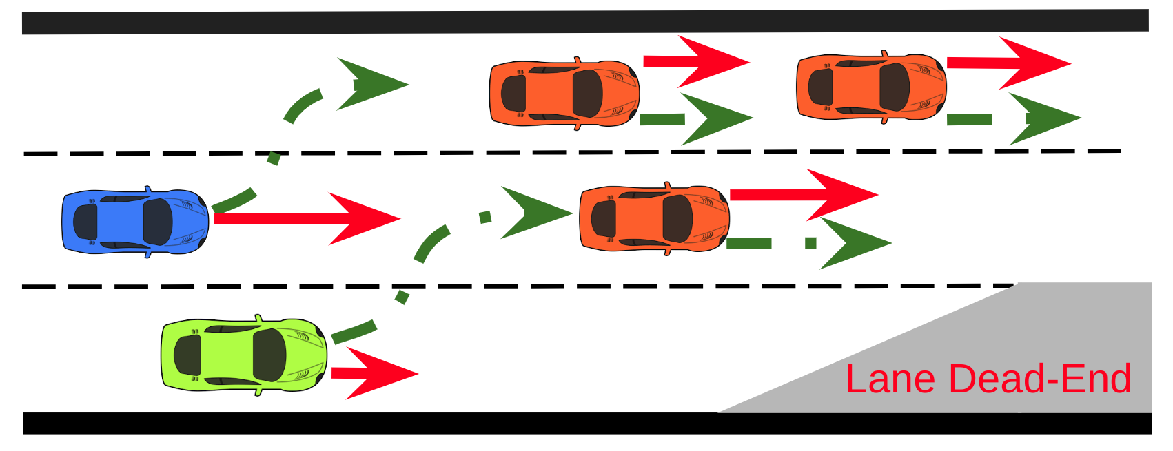
(a)

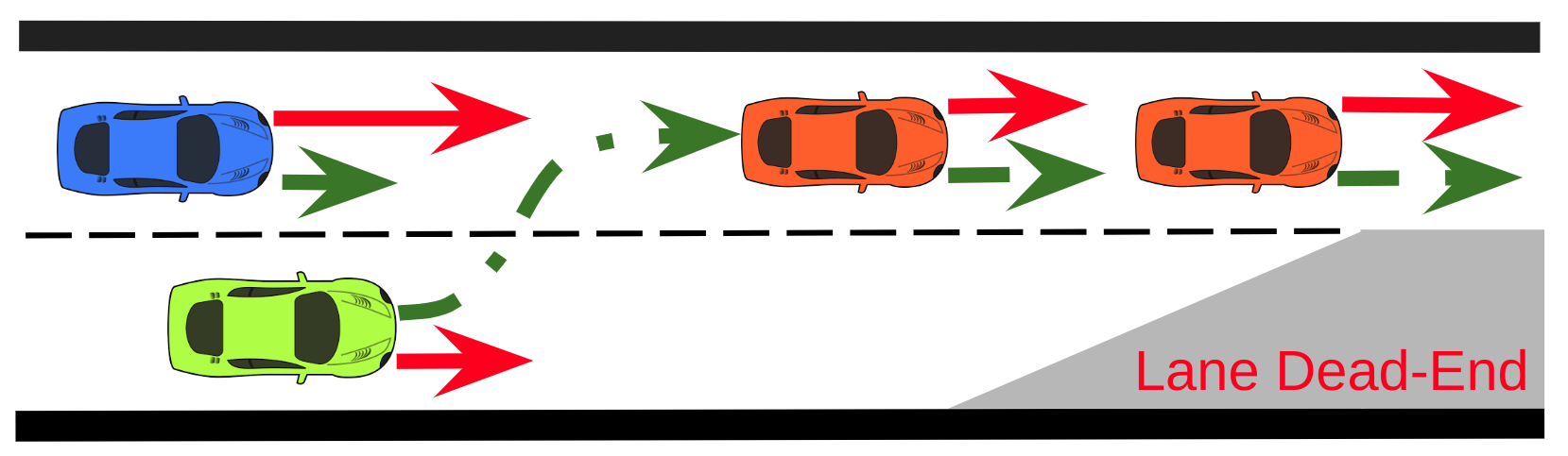
(b)

Figure 1: Dense traffic scenarios where the ego vehicle (green) intends to merge to the left lane. The red and green trajectories show the nominal (conservative) and interaction-aware trajectories for the ego vehicles, respectively, and correspondingly, their impact on the other vehicles. Due to interaction with the ego vehicle (green trajectory), in scenario (a), the blue vehicle switches lanes, and in scenario (b), the blue vehicle slows down to create space for the ego vehicle to perform a safe lane-change maneuver.

Reinforcement learning (RL) techniques [10] have been used to learn control policies under interactive or unknown environments. For example, adversarial RL is designed to reach the desired goal under uncertain conditions [11], and a model-free RL agent is developed for lane-changing control in dense traffic environments [12]. However, these RL methods are not yet appropriate for safety-critical AVs due to their low interpretability and reliability.

Designing interaction-aware planners presents a significant challenge, as predicting the reactions of surrounding vehicles to the ego vehicle’s actions is complex and non-trivial. Data-driven approaches, such as those using recurrent neural network architectures, have been effective in capturing the complex interactive behaviors of agents [13, 14], especially in predicting driver behavior with high accuracy and computational efficiency [14]. Therefore, it is desirable to utilize these data-driven methods to predict other vehicles’ interactive behavior while maintaining safety through rigorous control theory and established vehicle dynamics models.

We propose a model predictive control (MPC) based motion planner that incorporates AV’s decision and surrounding vehicles’ interactive behaviors into safety constraints to perform complex maneuvers. In particular, we provide a mathematical formulation for integrating the neural network’s predictions in the MPC controller and provide methods to obtain an (locally) optimal solution. However, the neural network integration and non-linear system dynamics make the optimization highly non-convex and challenging to solve analytically. Thus, prior efforts [6, 15, 9] that integrate neural network prediction into MPC are numerical in nature and rely on heuristic algorithms to generate a finite set of trajectory candidates. In [6] and [15], the authors generate these candidates by random sampling of control trajectories, and by generating spiral curves from source to target lane, respectively. In [9], the authors utilize a predefined set of reference trajectory candidates. Instead of solving the optimization, these approaches evaluate the cost of each candidate and choose the minimum cost trajectory that satisfies the safety constraint. Optimality is therefore restricted to trajectory candidates only, and the planner’s performance depends on the heuristic algorithm design. In contrast to these prior efforts, we avoid heuristics, detail a proper formalization, and solve the optimization with provable optimality. The optimal solution provides key insights to design better planners and can be leveraged to compare trajectories obtained by other heuristic methods.

The major contributions of this work are twofold: (i) we reformulate a highly complex MPC problem with a non-convex neural network and non-linear system dynamics, and systematically solve it using the Alternating Direction Method of Multiplier (ADMM) [16] with generic assumptions (Section III), and (ii) we investigate the mathematical properties of the ADMM algorithm for solving the MPC with an integrated neural network. Specifically, we provide sufficient conditions on the neural network such that the ADMM algorithm in non-convex optimization converges to a local optimum (Section IV). It is one of the first attempts in the literature toward provable mathematical guarantees for a neural network-integrated MPC.

II Problem Formulation and Controller Design

We design an MPC controller that leverages interactive behaviors of surrounding $N\in\mathbb{N}$ vehicles conditioned on the ego vehicle’s future actions. The key to leverage interactions is to integrate a neural network and interactively update controls with step-size $\Delta t\in\mathbb{R}_{>0}$ based on its inference (i.e., predicted positions during updates). This section further details the mathematical formulation of the MPC with the neural network.

Motivated by [17], we use bicycle kinematics. The corresponding states are $[$xy-coordinates, heading angle, speed$]$ denoted by $z(\tau)=[x(\tau),y(\tau),\psi(\tau),v(\tau)]^{\top}$ for all $\tau\in\{0,\ldots,T_{p}\}$ and the control inputs are $[$acceleration, steering angle$]$ denoted by $[a(\tau),\delta(\tau)]$ for all $\tau\in\{0,\ldots,T_{p}-1\}$ with the planning horizon $T_{p}\in\mathbb{N}$. For brevity, let $g(\tau)$ denote any general function $g(\cdot)$ at discrete time-step $\tau\in\mathbb{Z}_{\geq 0}$ with respect to (w.r.t) time $t$, i.e. $g(\tau)\equiv g(t+\tau\Delta t)$.

Then, at any time $t$, we solve the MPC to obtain the optimal control trajectories $\bm{\Delta^{\ast}}(t)\in\mathcal{D}\subset\mathbb{R}^{T_{p}}$ and $\bm{\alpha^{\ast}}(t)\in\mathcal{A}\subset\mathbb{R}^{T_{p}}$, and corresponding optimal state trajectory $\bm{Z}^{\ast}(t)\in\mathcal{Z}\subset\mathbb{R}^{4T_{p}}$, where:

$$\bm{\Delta^{\ast}}(t) =\begin{bmatrix}\delta^{\ast}(0),\ldots,\delta^{\ast}(T_{p}-1)\end{bmatrix}^{\top}, \mathcal{D}=[\delta_{min},\delta_{max}],$$

$$\bm{\alpha^{\ast}}(t) =\begin{bmatrix}a^{\ast}(0),\ldots,a^{\ast}(T_{p}-1)\end{bmatrix}^{\top}, \mathcal{A}=[a_{min},a_{max}],$$

$$\bm{Z}^{\ast}(t) =\begin{bmatrix}z^{\ast}(1),\ldots,z^{\ast}(T_{p})\end{bmatrix}^{\top}, \mathcal{Z}=[z_{min},z_{max}].$$

II-A Objective function

The controller’s objective is to move from the current lane to the desired lane as soon as possible while minimizing control effort and ensuring safety and smoothness. Let $x^{\text{ref}}$ denote the maximum longitude coordinate until when the ego must transition to the target lane. Let $\|\cdot\|$ denote the Euclidean norm. For $x<x^{\text{ref}}$, we utilize the following objective (cost) function $J(\bm{\Delta}(t),\bm{\alpha}(t),\bm{Z}(t))$ similar to [15]:

$$J =\sum_{\tau=1}^{T_{p}}\lambda_{div}\|y(\tau)-y^{\text{ref}}\|^{2}+\sum_{\tau=1}^{T_{p}}\lambda_{v}\|v(\tau)-v^{\text{ref}}\|^{2}\ \text{(error)}$$

$$+\sum_{\tau=0}^{T_{p}-1}\lambda_{\delta}\|\delta(\tau)\|^{2}+\sum_{\tau=0}^{T_{p}-1}\lambda_{a}\|a(\tau)\|^{2}\ \ \ \ \ \ \text{(control effort)}$$

$$+\sum_{\tau=0}^{T_{p}-1}\lambda_{\Delta\delta}\|\delta(\tau)-\delta(\tau-1)\|^{2}\ \ \ \ \ \ \ \ \ \ \ \ \ \text{(steering rate)}$$

$$+\sum_{\tau=0}^{T_{p}-1}\lambda_{\Delta a}\|a(\tau)-a(\tau-1)\|^{2},\ \ \ \ \ \ \ \ \ \ \ \ \ \ \ \ \ \ \ \ \ \text{(jerk)}$$

where $\bm{\Delta}(t)\in\mathcal{D}$, $\bm{\alpha}(t)\in\mathcal{A}$, and $\bm{Z}(t)\in\mathcal{Z}$ are the planned steering, acceleration, and state trajectories, respectively. $y^{\text{ref}}\in\mathbb{R}$ and $v^{\text{ref}}\in\mathbb{R}_{>0}$ are the reference latitude coordinate of the desired lane and desired velocity, respectively, provided by a high-level planner [18]. For a detailed description of each term, we refer the interested readers to [15].

II-B State Dynamics

Let $\tilde{\delta},\tilde{a}$ and $\tilde{z}$ be the last observed steering input, acceleration input and state of the ego vehicle, respectively. At any time $t$, we linearly approximate the discrete-time kinematic bicycle model [17] of the form $z(\tau+1)=f(\delta(\tau),a(\tau),z(\tau))$ about $(\tilde{\delta},\tilde{a},\tilde{z})$ to obtain the equality constraints for the optimization problem. We have

$$f(\delta(\tau),a(\tau),z(\tau)) \approx\tilde{A}\delta(\tau)+\tilde{B}a(\tau)+\tilde{C}z(\tau)+\tilde{D},$$ (1)

where $\tilde{A}\in\mathbb{R}^{4},\tilde{B}\in\mathbb{R}^{4},\tilde{C}\in\mathbb{R}^{4\times 4}$, and $\tilde{D}\in\mathbb{R}^{4}$ are constant matrices given by $\tilde{A}:=\frac{\partial f}{\partial\delta}\Big{|}_{(\tilde{\delta},\tilde{a},\tilde{z})}$, $\tilde{B}:=\frac{\partial f}{\partial a}\Big{|}_{(\tilde{\delta},\tilde{a},\tilde{z})}$, $\tilde{C}=\frac{\partial f}{\partial z}\Big{|}_{(\tilde{\delta},\tilde{a},\tilde{z})}$, and $\tilde{D}:=f(\tilde{\delta},\tilde{a},\tilde{z})-\tilde{A}\tilde{\delta}-\tilde{B}\tilde{a}-\tilde{C}\tilde{z}$, respectively. Hence, the linearized system dynamics is given by:

$$z(\tau+1)=\tilde{A}\delta(\tau)+\tilde{B}a(\tau)+\tilde{C}z(\tau)+\tilde{D}$$

$$\implies\tilde{A}\delta(\tau)+\tilde{B}a(\tau)+\tilde{C}z(\tau)-z(\tau+1)+\tilde{D}=0.$$ (2)

The equality constraints based on the system dynamics over the $T_{p}$ planning time-steps can be written as:

$$F(\bm{\Delta},\bm{\alpha},\bm{Z}):=A\bm{\Delta}+B\bm{\alpha}+C\bm{Z}+D=0,$$ (3)

where $A\in\mathbb{R}^{4T_{p}\times T_{p}},B\in\mathbb{R}^{4T_{p}\times T_{p}},C\in\mathbb{R}^{4T_{p}\times 4T_{p}}$, and $D\in\mathbb{R}^{4T_{p}}$ are constant matrices given by:

$$A =\begin{bmatrix}\tilde{A}&\bm{0}&\bm{0}&\cdots\\ \bm{0}&\tilde{A}&\bm{0}&\cdots\\ \vdots&\vdots&\vdots&\cdots\end{bmatrix},\ B=\begin{bmatrix}\tilde{B}&\bm{0}&\bm{0}&\cdots\\ \bm{0}&\tilde{B}&\bm{0}&\cdots\\ \vdots&\vdots&\vdots&\cdots\end{bmatrix},$$

$$C =\begin{bmatrix}-\bm{I}&\bm{0}&\bm{0}&\cdots\\ \tilde{C}&-\bm{I}&\bm{0}&\cdots\\ \bm{0}&\tilde{C}&-\bm{I}&\cdots\\ \vdots&\vdots&\vdots&\cdots\end{bmatrix},\ D=\begin{bmatrix}\tilde{D}-\tilde{C}z(0)\\ \tilde{D}\\ \tilde{D}\\ \vdots\end{bmatrix},$$ (4)

$\bm{0}$ and $\bm{I}$ denote the zero and identity matrix, respectively.

Remark 1

To simplify the optimization, we linearly approximate the system dynamics before solving the MPC. This is possible because the control inputs obtained through the MPC are only applied for a single time-step, using a receding horizon control approach [19]. As a result, any linearization errors from previous time-steps do not affect the MPC optimization.

II-C Safety Constraints

The safety constraints for collision avoidance depend on the nearby vehicles’ trajectory prediction and the vehicle shape model. Let $\mathcal{V}$ denote the set of nearby vehicles surrounding the ego vehicle. Let $\phi(\tau)$ be a trained neural network that jointly predicts the future trajectories of the ego vehicle and its surrounding vehicles for $T_{pred}$ time-steps into the future based on their trajectories for $T_{obs}$ time-steps in the past. $\phi(\tau)$ is given by:

$$\phi(\tau): \begin{bmatrix}(x(\tau),y(\tau))&\cdots&(x_{N}(\tau),y_{N}(\tau))\\ \vdots&\vdots&\vdots\\ \begin{matrix}(x(\tau-T_{obs}+1),\\ \ y(\tau-T_{obs}+1))\end{matrix}&\cdots&\begin{matrix}(x_{N}(\tau-T_{obs}+1),\\ \ y_{N}(\tau-T_{obs}+1))\end{matrix}\end{bmatrix}$$

$$\hskip 113.81102pt\downarrow$$

$$\!\!\!\!\!\!\begin{bmatrix}(\hat{x}(\tau+1),\hat{y}(\tau+1))&\cdots&(\hat{x}_{N}(\tau+1),\hat{y}_{N}(\tau+1))\end{bmatrix},$$

with $T_{pred}=1$, where the first column represents the positions of the ego vehicle followed by the positions of $N$ surrounding vehicles. Given the buffer of $T_{obs}$ past observations until time-step $\tau$, the coordinates of vehicle $i\in\mathcal{V}$ at time-step $\tau+1$ are represented as:

$$\hat{x}_{i}(\tau+1)=\phi_{i,x}(\tau),\ \qquad\hat{y}_{i}(\tau+1)=\phi_{i,y}(\tau).$$ (5)

Some examples of the neural network $\phi(\tau)$ include social generative adversarial network (SGAN) [14] and graph-based spatial-temporal convolutional network (GSTCN) [20].

Remark 2

Interactive predictions over planning horizon $T_{p}$ are computed recursively using $\phi(t)$ with $T_{pred}=1$ based on the latest reactive predictions and ego vehicle positions from the MPC’s candidate solution trajectory.

We model the vehicle shape using a single circle to obtain a smooth and continuously differentiable distance measure to enable gradient-based optimization methods. Let $(x,y)$ and $(\hat{x}_{i},\hat{y}_{i})$ be the position of the ego vehicle and the predicted positions of the surrounding vehicles $i\in\mathcal{V}$ (obtained using $\phi(\tau)$), respectively. Let $r,r_{i}\in\mathbb{R}_{>0}$ be the radius of circles modeling ego vehicle and vehicle $i$, respectively. The safety constraint for the ego vehicle w.r.t vehicle $i$ then reads:

$$d_{i}(x,y,\hat{x}_{i},\hat{y}_{i}) ={(x-\hat{x}_{i})^{2}+(y-\hat{y}_{i})^{2}}$$

$$\quad\quad\quad\quad\quad-(r+r_{i}+\epsilon)^{2}>0,$$ (6)

where $\epsilon\in\mathbb{R}_{>0}$ is a safety bound.

Remark 3

Using the single circle model, the safety constraints can be conservative, and consequently, the feasible solutions could be restrictive in some situations. We use it for its simplicity and to reduce the number of safety constraints. Some other alternatives for modeling the vehicle shape include the ellipsoid model [21] and three circle model [6].

II-D Formulation of the Optimization problem

We now present the complete optimization problem for the receding horizon control in a compact form:

$$\min_{\bm{\Delta},\bm{\alpha},\bm{Z}}\;\;J= \Phi_{1}(\bm{\Delta})+\Phi_{2}(\bm{\alpha})+\Phi_{3}(\bm{Z}),$$ (7)

subject to $$F(\bm{\Delta},\bm{\alpha},\bm{Z})=0,\ \ \ b_{i}(\bm{Z})>0,\ i\in\mathcal{V},$$ (8)

$$\bm{\Delta}\in\mathcal{D},\bm{\alpha}\in\mathcal{A},\bm{Z}\in\mathcal{Z},\ \text{where}$$ (9)

$$\ \Phi_{1}(\bm{\Delta})=\sum_{\tau=0}^{T_{p}-1} \lambda_{\delta}\|\delta(\tau)\|^{2}+\sum_{\tau=0}^{T_{p}-1}\lambda_{\Delta\delta}\|\delta(\tau)-\delta(\tau-1)\|^{2},$$

$$\ \Phi_{2}(\bm{\alpha})=\sum_{\tau=0}^{T_{p}-1} \lambda_{a}\|a(\tau)\|^{2}+\sum_{\tau=0}^{T_{p}-1}\lambda_{\Delta a}\|a(\tau)-a(\tau-1)\|^{2},$$

$$\ \Phi_{3}(\bm{Z})=\sum_{\tau=1}^{T_{p}} \lambda_{div}\|y(\tau)-y^{\text{ref}}\|^{2}+\sum_{\tau=1}^{T_{p}}\lambda_{v}\|v(\tau)-v^{\text{ref}}\|^{2},$$

$$\!\!\!\!\!\!\!\!\!\!\!\!\!\!\!\!\!\!\!\!\!\!\!\!\!\!\!\!\!\!\!\!\!\!\!\!b_{i}(\bm{Z})=\begin{bmatrix}d_{i}(x(1),y(1),\phi_{i,x}(0),\phi_{i,y}(0))\\ \vdots\\ d_{i}(x(T_{p}),y(T_{p}),\phi_{i,x}(T_{p}-1),\phi_{i,y}(T_{p}-1))\\ \end{bmatrix}.$$

In the next section, we solve the optimization using ADMM to determine a safe and interactive ego vehicle’s trajectory.

III Solving MPC with ADMM

There are many mathematical challenges associated with the MPC problem in Section II. Namely, it has the non-linear system dynamics, non-convex safety constraints, and dependence of the neural network predictions on its predictions in previous time steps ($T_{obs}\neq 1$). We now detail the systematic steps to solve the complex problem using ADMM, addressing the aforementioned mathematical challenges.

First, we construct a Lagrangian by moving the safety constraints, $b_{i}(\bm{Z})>0,\ i\in\mathcal{V}$, in the optimization objective:

$$\!\!\!\min_{\bm{\Delta},\bm{\alpha},\bm{Z}}J= \Phi_{1}(\bm{\Delta})+\Phi_{2}(\bm{\alpha})+\Phi_{3}(\bm{Z})-\sum_{i=1}^{N}\lambda_{s}^{T}b_{i}(\bm{Z}),$$ (10)

$$\text{subject to }\;\ F(\bm{\Delta},\bm{\alpha},\bm{Z})=0,$$ (11)

$$\bm{\Delta}\in\mathcal{D},\bm{\alpha}\in\mathcal{A},\bm{Z}\in\mathcal{Z},$$ (12)

where $\lambda_{s}\in\mathbb{R}^{T_{p}}_{>0}$ is the vector of Lagrange multipliers.

Remark 4

For theoretical analysis, we incorporate safety constraints into the optimization objective, but for our simulation study, we enforce them as hard constraints.

The optimization problem (10)-(12) is separable and the optimization variables $\bm{\Delta},\bm{\alpha},\bm{Z}$ are decoupled in the objective function. Following the convention in [22], the augmented Lagrangian is given by:

$$\mathcal{L}_{\rho}(\bm{\Delta},\bm{\alpha},\bm{Z})=\Phi_{1}(\bm{\Delta})+\Phi_{2}(\bm{\alpha})+\Phi_{3}(\bm{Z})-\sum_{i=1}^{N}\lambda_{s}^{T}b_{i}(\bm{Z})+\\ \mu^{\top}F(\bm{\Delta},\bm{\alpha},\bm{Z})+\left(\frac{\rho}{2}\right)\|F(\bm{\Delta},\bm{\alpha},\bm{Z})\|^{2},$$ (13)

where $\rho>0$ is the ADMM Lagrangian parameter and $\mu$ is the dual variable associated with the constraint (11). The complete algorithm is given by the Algorithm 1.

Init : states $z=z_{0}$, controls $\delta=\delta_{0},a=a_{0}$

Surrounding vehicles’ position:

$(x_{i},y_{i})=(x_{i,0},y_{i,0})$ for all $i\in\mathcal{V}$

1 while $x<x^{\text{ref}}$ and $y\neq y^{\text{ref}}$ do

2       Find the optimal control that minimizes the cumulative cost over horizon $T_{p}$

       Init : $\bm{\hat{\Delta}}=\bm{\Delta}_{0},\bm{\hat{\alpha}}=\bm{\alpha}_{0},\bm{\hat{Z}}=\bm{Z}_{0},\hat{\mu}=\mu_{0}$

3       while convergence criterion is not met do

4             $\bm{\hat{\Delta}}\leftarrow\operatorname{argmin}_{\bm{\Delta}}\mathcal{L}_{\rho}(\bm{\Delta},\bm{\hat{\alpha}},\bm{\hat{Z}})$

5             $\bm{\hat{\alpha}}\leftarrow\operatorname{argmin}_{\bm{\alpha}}\mathcal{L}_{\rho}(\bm{\hat{\Delta}},\bm{\alpha},\bm{\hat{Z}})$

6             $\hat{\bm{Z}}\leftarrow\operatorname{argmin}_{\bm{Z}}\mathcal{L}_{\rho}(\bm{\hat{\Delta}},\bm{\hat{\alpha}},\bm{Z})$

7             $\hat{\mu}\leftarrow\hat{\mu}+\rho(F(\bm{\hat{\Delta}},\bm{\hat{\alpha}},\bm{\hat{Z}}))$

8            

9       end while

10      

11      Update the states through non-linear state dynamics with first elements of controls

12       $z\leftarrow f([\bm{\hat{\Delta}}]_{0},[\bm{\hat{\alpha}}]_{0},z)$

13      

14      Observe positions of other vehicles at the current time $t$

15       $(x_{i},y_{i})\leftarrow(x_{i}(t),y_{i}(t))$ for all $i$

16 end while

Algorithm 1 MPC with ADMM

Next, we provide details for solving each of the local optimization problems at iteration $k$, for solving the MPC.

III-A Update $\bm{\Delta}^{(k+1)}=\operatorname{argmin}_{\bm{\Delta}\in\mathcal{D}}\;\mathcal{L}_{\rho}(\bm{\Delta},\bm{\alpha}^{(k)},\bm{Z}^{(k)})$

The sub-optimization problem for $\bm{\Delta}^{(k+1)}$ is given by

$$\operatorname{argmin}_{\bm{\Delta}}\ \sum_{\tau=0}^{T_{p}-1}\lambda_{\delta}\|\delta(\tau)\|^{2}+\sum_{\tau=0}^{T_{p}-1}\lambda_{\Delta\delta}\|\delta(\tau)-\delta(\tau-1)\|^{2}$$

$$\quad\quad\quad\quad\quad\quad+\mu^{k\top}A\bm{\Delta}+\left(\frac{\rho}{2}\right)\|A\bm{\Delta}-c_{\bm{\Delta}}^{(k)}\|^{2},$$ (14)

$$\text{subject to}\;\;\;\delta(\tau)\in[\delta_{\min},\delta_{\max}],$$

where $c_{\bm{\Delta}}^{(k)}=A\bm{\Delta}^{(k)}-F(\bm{\Delta}^{(k)},\bm{\alpha}^{(k)},\bm{Z}^{(k)})$. It is a convex problem; hence, we can use a canonical convex optimization algorithm [22] to find the optimal solution.

III-B Update $\bm{\alpha}^{(k+1)}=\operatorname{argmin}_{\bm{\alpha}\in\mathcal{A}}\;\mathcal{L}_{\rho}(\bm{\Delta}^{(k+1)},\bm{\alpha},\bm{Z}^{(k)})$

The sub-optimization problem for $\bm{\alpha}^{(k+1)}$ is given by

$$\operatorname{argmin}_{\bm{\alpha}}\sum_{\tau=0}^{T_{p}-1}\lambda_{a}\|a(\tau)\|^{2}+\sum_{\tau=0}^{T_{p}-1}\lambda_{\Delta a}\|a(\tau)-a(\tau-1)\|^{2}$$

$$\quad\quad\quad\quad\quad\quad+\mu^{k\top}B\bm{\alpha}+\left(\frac{\rho}{2}\right)\|B\bm{\alpha}-c_{\bm{\alpha}}^{(k)}\|^{2},$$ (15)

$$\text{subject to}\;\;\;a(\tau)\in[a_{\min},a_{\max}],$$

where $c_{\bm{\alpha}}^{(k)}=B\bm{\alpha}^{(k)}-F(\bm{\Delta}^{(k+1)},\bm{\alpha}^{(k)},\bm{Z}^{(k)})$. It is a convex problem; hence, we can use a canonical convex optimization algorithm [22] to find the optimal solution.

III-C Update $\bm{Z}^{(k+1)}=\operatorname{argmin}_{\bm{Z}\in\mathcal{Z}}\;\mathcal{L}_{\rho}(\bm{\Delta}^{(k+1)},\bm{\alpha}^{(k+1)},\bm{Z})$

The sub-optimization problem for $\bm{Z}^{(k+1)}$ is given by

$$\operatorname{argmin}_{\bm{Z}}\sum_{\tau=1}^{T_{p}}\lambda_{div}\|y(\tau)-y^{\text{ref}}\|^{2}+\sum_{\tau=1}^{T_{p}}\lambda_{v}\|v(\tau)-v^{\text{ref}}\|^{2}$$

$$\quad-\sum_{i=1}^{N}\lambda_{s}^{T}b_{i}(\bm{Z})+\mu^{k\top}C\bm{Z}+\left(\frac{\rho}{2}\right)\|C\bm{Z}-c_{\bm{Z}}^{(k)}\|^{2},$$ (16)

$$\text{subject to }z(\tau)\in[z_{\min},z_{\max}],$$ (17)

where $c_{\bm{Z}}^{(k)}=C\bm{Z}^{(k)}-F(\bm{\Delta}^{(k+1)},\bm{\alpha}^{(k+1)},\bm{Z}^{(k)})$. Due to the nonconvexity of the neural network in $b_{i}(\bm{Z})$, the objective function (16) is non-convex. We prefer the Quasi-Newton method for optimization to avoid expensive Hessian computation at each step. Hence, we utilize BFGS-SQP method [23], which employs BFGS Hessian approximations within a sequential quadratic optimization, and does not assume any special structure in the objective or constraints. For a solver, we use PyGranso [24], a PyTorch-enabled port of GRANSO, that enables gradients computation by back-propagating the neural network’s gradients at each iteration.

Remark 5

The state trajectory $\bm{Z}$ update has a larger complexity in the problem due to the presence of the non-convex neural network predictions. To expedite the $\bm{Z}$ update, an offline-trained function approximator such as a neural network can be utilized to estimate the gradients of the original neural network. The training dataset for gradient approximator can be generated using automatic differentiation or central differences approximations with original network.

Henceforth, we refer to our method as ADMM-NNMPC.

IV Convergence of MPC with ADMM

Due to the inherent non-convexity of the neural network, the rigorous convergence analysis of ADMM in [16] is not readily applicable. Thus, we extend the convergence analysis of ADMM with an integrated neural network, i.e., the convergence of the inner while loop in Algorithm 1. We first make the following assumptions on the neural network:

1. At any time-step $\tau\in[0,T_{p}]$, the neural network’s outputs are bounded, i.e. $|\phi_{i,x}(\tau)|\leq s_{x}$ and $|\phi_{i,y}(\tau)|\leq s_{y}$, $i\in\mathcal{V}$, where $s_{x},s_{y}\in\mathbb{R}_{>0}$ are constants.

2. At any time-step $\tau\in[0,T_{p}]$, the gradients of the neural network’s outputs w.r.t the input ego trajectory exist and are bounded, i.e. $\|\frac{\partial{\phi_{i,x}}(t)}{\partial\bm{Z}}\|_{\infty}\leq\theta_{x}$ and $\|\frac{\partial{\phi_{i,y}(t)}}{\partial\bm{Z}}\|_{\infty}\leq\theta_{y}$ for all $i\in\mathcal{V}$, where $\theta_{x},\theta_{y}\in\mathbb{R}_{>0}$ are constants and $\|\cdot\|_{\infty}$ is the max. norm of a vector.

3. At any time-step $\tau\in[0,T_{p}]$, the neural network’s outputs are Lipschitz differentiable, i.e. $||\nabla\phi_{i,x}(\bm{Z}_{1})-\nabla\phi_{i,x}(\bm{Z}_{2})||\leq L_{\nabla\phi}||\bm{Z}_{1}-\bm{Z}_{2}||$ and $||\nabla\phi_{i,y}(\bm{Z}_{1})-\nabla\phi_{i,y}(\bm{Z}_{2})||\leq L_{\nabla\phi}||\bm{Z}_{1}-\bm{Z}_{2}||$ for all $i\in\mathcal{V}$, $\bm{Z}_{1},\bm{Z}_{2}\in\mathcal{Z}$, where $L_{\nabla\phi}\in\mathbb{R}_{>0}$ is the Lipschitz constant for the neural network’s gradient.

Assumptions (A1)-(A3) are sufficient conditions under which the objective function (10) is Lipschitz differentiable, i.e., it is differentiable and its gradient is Lipschitz continuous. This allows us to establish the convergence of Algorithm 1. Assumption (A1) is satisfied for a trained neural network for a bounded input space. Furthermore, neural network outputs can be clipped based on the feasible region. Lastly, neural networks with $C^{2}$ activation functions such as Gaussian Error Linear Unit (GELU) [25] and Smooth Maximum Unit (SMU) [26] satisfy assumptions (A2)-(A3).

Remark 6

Assumptions (A1)-(A3) are sufficient conditions and not necessary conditions. If the neural network architecture is unknown or it doesn’t satisfy the assumptions, knowledge distillation [27] can be used to train a smaller (student) network that satisfies the assumptions from the large (teacher) pre-trained network.

Theorem 1

[Convergence of MPC with ADMM] Under the assumptions (A1)–(A3), the inner while loop in Algorithm 1 converges subsequently for any sufficiently large $\rho>\max\{1,(1+2\sigma_{\min}(C))L_{J}M\}$, where $\sigma_{\min}(C)$ is the smallest positive singular value of $C$ in (II-B), $L_{J}$ is the Lipschitz constant for $J$ in (10), and $M$ is the Lipschitz constant for sub-minimization paths as defined in Lemma 2. Therefore, starting from any $\bm{\Delta}^{(0)},\bm{\alpha}^{(0)},\bm{Z}^{(0)},\mu^{(0)}$, it generates a sequence that is bounded, has at least one limit point, and that each limit point $\bm{\Delta}^{*},\bm{\alpha}^{*},\bm{Z}^{*},\mu^{*}$ is a stationary point of $\mathcal{L}_{\rho}$ satisfying $\nabla\mathcal{L}_{\rho}(\bm{\Delta}^{*},\bm{\alpha}^{*},\bm{Z}^{*},\mu^{*})=0$.

We prove Theorem 1 using Lemmas 1-3.

Lemma 1

[Feasibility] Let $Q:=[A,B]$. Then $\text{Im}(Q)$ $\subseteq\text{Im}(C)$, where $\text{Im}(\cdot)$ returns the image of a matrix, and $A,B,$ and $C$ is defined in (II-B).

Proof:

See Appendix -A for the proof. ∎

Lemma 2

[Lipschitz sub-minimization paths] The following statements hold for the optimization problem:

1. For any fixed $\bm{\alpha},\bm{Z}$, $H_{1}:Im(A)\rightarrow\mathbb{R}^{T_{p}}$ defined by $H_{1}(u)\triangleq\operatorname{argmin}_{\bm{\Delta}}\{J(\bm{\Delta},\bm{\alpha},\bm{Z}):A\bm{\Delta}=u\}$ is unique and a Lipschitz continuous map.

2. For any fixed $\bm{\Delta},\bm{Z}$, $H_{2}:Im(B)\rightarrow\mathbb{R}^{T_{p}}$ defined by $H_{2}(u)\triangleq\operatorname{argmin}_{\bm{\alpha}}\{J(\bm{\Delta},\bm{\alpha},\bm{Z}):B\bm{\alpha}=u\}$ is unique and a Lipschitz continuous map.

3. For any fixed $\bm{\Delta},\bm{\alpha}$, $H_{3}:Im(C)\rightarrow\mathbb{R}^{4T_{p}}$ defined by $H_{3}(u)\triangleq\operatorname{argmin}_{\bm{Z}}\{J(\bm{\Delta},\bm{\alpha},\bm{Z}):C\bm{Z}=u\}$ is unique and a Lipschitz continuous map,

where $A,B,$ and $C$ is defined in (II-B). Moreover, $H_{1},H_{2},H_{3}$ have a universal Lipschitz constant $M>0$.

Proof:

See Appendix -B for the proof. ∎

Lemma 3

[Lipschitz Differentiability] Under the assumptions (A1)-(A3), the objective function $J(\bm{\Delta},\bm{\alpha},\bm{Z})$ in (10) is Lipschitz differentiable.

Proof:

See Appendix -C for the proof. ∎

Proof of Theorem 1: See Appendix -D for the proof. $\hfill\blacksquare$

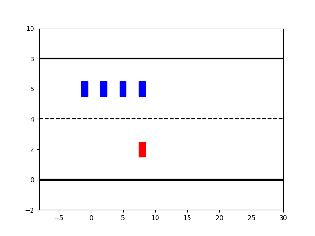
(a) $t=0$

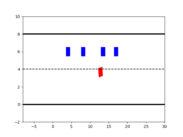
(b) $t=5$

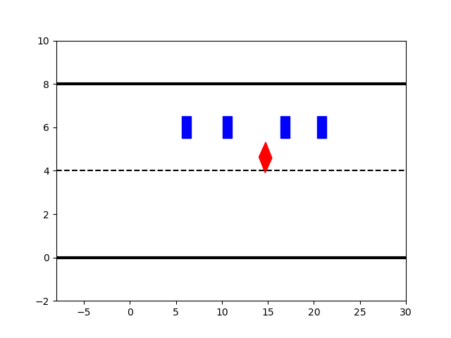
(c) $t=11$

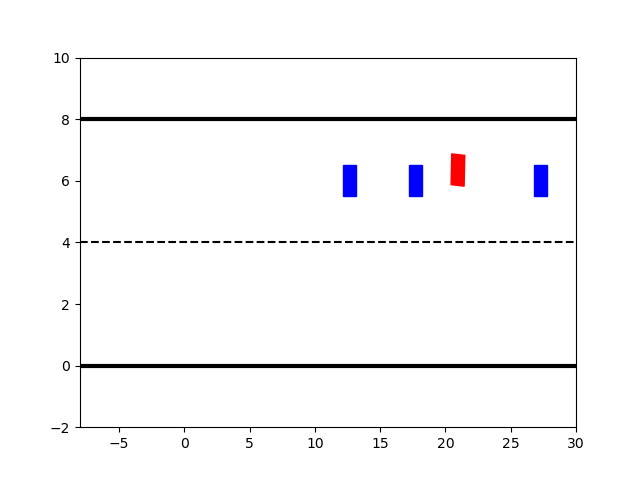
(d) $t=13$

Figure 2: Two lane scenario: (a)-(d) shows the ADMM-NNMPC solution in a two-lane scenario after $0,5,7,$ and $13$ time steps, respectively. The ego vehicle (red) opens a gap by nudging the vehicles to change their speeds.

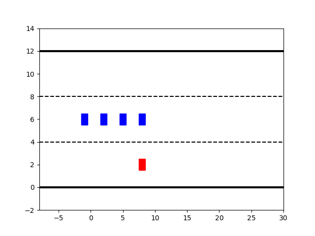
(a) $t=0$

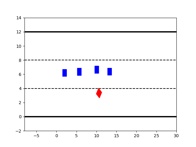
(b) $t=3$

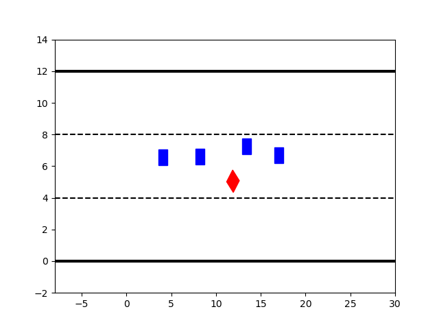
(c) $t=5$

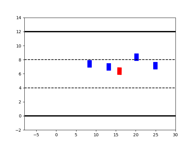
(d) $t=9$

Figure 3: Three lane scenario: (a)-(d) shows the ADMM-NNMPC solution in a three-lane scenario after $0,3,5,$ and $9$ time steps, respectively. The ego vehicle (red) opens a gap for itself by nudging the vehicles to transition into the left-most lane.

Param	Description	Value
$\lambda_{div}$	Weight on divergence from target lane	1.0
$\lambda_{v}$	Weight on divergence from target speed	1.0
$\lambda_{\delta}$	Weight on steering angle	0.6
$\lambda_{a}$	Wight on acceleration	0.4
$\lambda_{\Delta\delta}$	Weight on steering rate	0.4
$\lambda_{\Delta a}$	Weight on jerk	0.2
$\rho$	ADMM Lagrangian parameter	100

TABLE I: Objective function coefficients

	Two-Lane Scenario		Three-Lane Scenario
	NNMPC	ADMM-NNMPC	NNMPC	ADMM-NNMPC
$t_{merge}$	Fails after 17	9	29	7
$C_{\max}$	80.9	62	114.6	53.3
$d_{\min}$	0.91	2.41	2.97	2.66

TABLE II: Simulation results for ADMM-NNMPC and NNMPC in the two-lane and three-lane scenario. $t_{merge}$ are the number of time steps taken by the ego vehicle to merge into the target lane. $C_{\max}$ and $d_{\min}$ are the maximum cost and minimum distance between the ego vehicle and other vehicles at any point of the simulation, respectively.

V Simulation Study

We now present the simulation results for ADMM-NNMPC. Figure 2 and 3 show the vehicles’ positions at different time steps in two scenarios in which the ego vehicle (red) intends to merge into the left lane which is occupied by four other vehicles (blue) with a narrow inter-vehicle gap. In the two-lane scenario (Fig. 2), other vehicles can only change their speeds, while in the three-lane scenario (Fig. 3), other vehicles can also move laterally to transition into the leftmost lane. The other vehicles’ positions at different time steps match the neural network’s predictions, and hence, the ego vehicle’s actions affect the trajectory of the other vehicles. In both scenarios, the ego vehicle is able to interact with the other agents and open a gap for itself to merge into.

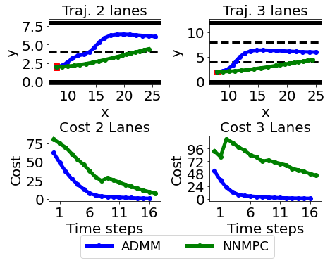
(a)

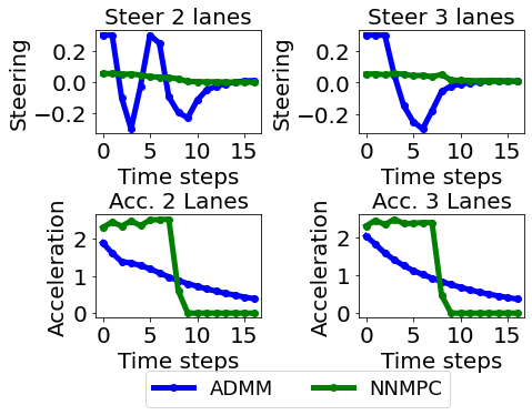
(b)

Figure 4: (a) compares the trajectory (top) and cost (bottom) of the ADMM-NNMPC and NNMPC solutions in the two-lane (left) and three-lane (right) scenarios until $x_{ref}=25$. (b) compares the steering (top) and acceleration (bottom) trajectories for ADMM-NNMPC and NNMPC solutions in the two-lane (left) and three-lane (right) scenarios.

We compare ADMM-NNMPC with a baseline method called NNMPC [15] on the two-lane and three-lane scenarios by utilizing the same cost function (cost function coefficients listed in Table I) and $T_{p}=8$ time steps. NNMPC generates trajectory candidates by computing a finite set of spiral curves from the source lane to the target lane and selects the candidate with minimum cost. In both methods, we use a trained SGAN neural network [14] for interactive motion prediction of the other vehicles. Table II compares the simulation results for the baseline NNMPC and ADMM-NNMPC in the two-lane and three-lane scenarios. In the two-lane scenario, while the ADMM-NNMPC successfully merges in the left lane, the NNMPC method fails to make a lane change due to limited trajectory candidates. In the three-lane scenario, ADMM-NNMPC successfully switches lanes much faster than NNMPC. Furthermore, ADMM-NNMPC outperforms NNMPC in terms of maximum cost and minimum distance from other vehicles in both scenarios.

Figure 4(a) compares the trajectory (top) and cost (bottom) of the ADMM-NNMPC and NNMPC solutions in the two-lane (left) and three-lane (right) scenarios until $x_{ref}=25$. In both scenarios, while ADMM-NNMPC successfully merges into the left lane, NNMPC fails to switch lanes before $x_{ref}$ due to limited trajectory candidates. Furthermore, the ADMM-NNMPC’s cost is lower than the NNMPC solution at every time step since ADMM-NNMPC solves the optimization. Figure 4(b) compares the steering (top) and acceleration (bottom) trajectories for ADMM-NNMPC and NNMPC solutions in the two-lane (left) and three-lane (right) scenarios. Since ADMM-NNMPC solves for the optimal solution, it actively interacts with the other vehicles to open a gap for itself to merge into. Therefore, the steering trajectory in ADMM-NNMPC is more aggressive that the NNMPC. Lastly, the acceleration gradually changes in ADMM-NNMPC to reach the desired speed while minimizing jerk.

V-A Limitations and Future Works

Although we reduce the problem complexity by decomposing it into smaller sub-problems, these sub-problems are still complex which makes the approach non-scalable. Furthermore, due to the large neural network size and re-computation of gradients at each iteration, our current implementation runs slower than real-time. Nevertheless, having a slow offline optimization is useful, as it can serve as a benchmark when developing faster heuristic methods, ideally, we would like to increase the efficiency. Our approach can be made faster by training another neural network to estimate the original neural network’s gradients and developing faster optimization libraries. Thus, future works include: (i) designing a smaller network trained with knowledge distillation [27], or (ii) expediting neural network’s gradient estimation using an offline-trained function approximator such as a neural network.

VI Conclusions

With the importance of motion planning strategies being interaction-aware, e.g., lane changing in dense traffic for autonomous vehicles, this paper investigates mathematical solutions of a model predictive control with a neural network that estimates interactive behaviors. The problem is highly complex due to the non-convexity of the neural network, and we show that the problem can be effectively solved by decomposing it into sub-problems by leveraging the alternating direction method of multipliers (ADMM). This paper further examines the convergence of ADMM in presence of the neural network, which is one of the first attempts in the literature. The simple numerical study supports the provably optimal solutions being effective. The computational burden due to the complexity is still a limitation, and improving the computation efficiency remains for future work. That said, having a provably optimal solution is valuable as a benchmark when developing heuristic methods.

-A Proof of Lemma 1

$C$ in (II-B) is a lower triangular matrix with diagonal entries as $-1$. Hence, $C$ is a full rank matrix of rank $4T_{p}$, and $\text{Im}(C)=\mathbb{R}^{4T_{p}}$. We have, $\text{Im}(Q)=\{y\in\mathbb{R}^{4T_{p}}|\ y=Qx=[A,B]x\ \text{such that }x\in\mathbb{R}^{2T_{p}}\}\subseteq\mathbb{R}^{4T_{p}}=\text{Im}(C)$. $\hfill\blacksquare$

-B Proof of Lemma 2

$A$ and $B$ are full column rank matrices of column rank $T_{p}$. Furthermore, $C$ is a full rank matrix of rank $4T_{p}$. Therefore, their null spaces are trivial, and hence, $H_{1},H_{2},H_{3}$ reduces to linear operators and satisfies the Lemma. $\hfill\blacksquare$

-C Proof of Lemma 3

$\Phi_{1}(\bm{\Delta})$, $\Phi_{2}(\bm{\alpha})$, and $\Phi_{3}(\bm{Z})$ are $C^{2}$ functions, and hence, Lipschitz differentiable. Therefore, to show the Lipschitz differentiability of $J$, it is sufficient to show that $b_{i}(\bm{Z})$, $i\in\mathcal{V}$, is Lipschitz differentiable for any $\tau\in\{1,\ldots,T_{p}\}$. For brevity of space, we define our notations in terms of $w\in\{x,y\}$ where $w$ can either be $x$ or $y$. Let $q_{w}(\tau):=2(w(\tau)-\phi_{i,w}(\tau-1))$. We have

$$\frac{\partial b_{i}(\bm{Z})}{\partial x(k)}=\begin{cases}-q_{x}(\tau)\frac{\partial\phi_{i,x}(\tau-1)}{\partial x(k)}-\\ \quad q_{y}(\tau)\frac{\partial\phi_{i,y}(\tau-1)}{\partial x(k)},\ \text{for}\ k\leq\tau-1\\ q_{x}(\tau),\ \ \ \ \text{for}\ k=\tau\\ 0,\ \ \ \ \text{for}\ k\in\{\tau+1,\ldots,T_{p}\}.\end{cases}$$

Let $T^{w}_{k}:=\left|\frac{\partial b_{i}(\bm{Z}_{1})}{\partial w(k)}-\frac{\partial b_{i}(\bm{Z}_{2})}{\partial w(k)}\right|$ for some $\bm{Z}_{1},\bm{Z}_{2}\in\mathcal{Z}$, and let $(x^{m}(\tau),y^{m}(\tau))$ denote the ego vehicle positions in $\bm{Z}_{m}$, where $m\in\{1,2\}$. Let $\phi_{i,w}^{\bm{Z}_{m}}$ denote $\phi_{i,w}$ corresponding to $\bm{Z}_{m}$. Using assumption (A2) and mean-value theorem [28], the neural network’s outputs are Lipschitz continuous, i.e., $\|\phi_{i,w}^{\bm{Z}_{1}}-\phi_{i,w}^{\bm{Z}_{2}}\|\leq\theta_{w}||\bm{Z}_{1}-\bm{Z}_{2}||$. Let $\Delta w(\tau)=|w^{1}(\tau)-w^{2}(\tau)|$, $\varphi_{w}(\tau-1)=|\phi_{i,w}^{\bm{Z}_{2}}(\tau-1)-\phi_{i,w}^{\bm{Z}_{1}}(\tau-1)|$, and $\nu^{w}_{x}(\tau-1)=\Bigg{|}\frac{\partial\phi_{i,w}^{\bm{Z}_{1}}(\tau-1)}{\partial x(k)}-\frac{\partial\phi_{i,w}^{\bm{Z}_{2}}(\tau-1)}{\partial x(k)}\Bigg{|}$. For any $k\in\{1,\ldots,\tau-1\}$:

$$T_{k}^{x} \leq 2\Delta x(\tau)\Bigg{|}\frac{\partial\phi_{i,x}^{\bm{Z}_{1}}(\tau-1)}{\partial x(k)}\Bigg{|}+2\Delta y(\tau)\Bigg{|}\frac{\partial\phi_{i,y}^{\bm{Z}_{1}}(\tau-1)}{\partial x(k)}\Bigg{|}+$$

$$\quad\quad 2|x^{2}(\tau)|\nu^{x}_{x}(\tau-1)+2\varphi_{x}(\tau-1)\Bigg{|}\frac{\partial\phi_{i,x}^{\bm{Z}_{2}}(\tau-1)}{\partial x(k)}\Bigg{|}+$$

$$\quad\quad 2|y^{2}(\tau)|\nu^{y}_{x}(\tau-1)+2\varphi_{y}(\tau-1)\Bigg{|}\frac{\partial\phi_{i,y}^{\bm{Z}_{2}}(\tau-1)}{\partial x(k)}\Bigg{|}+$$

$$\quad\quad 2|\phi_{i,x}^{\bm{Z}_{1}}(\tau-1)|\nu^{x}_{x}(\tau-1)+2|\phi_{i,y}^{\bm{Z}_{1}}(\tau-1)|\nu^{y}_{x}(\tau-1)$$

$$\leq 2\theta_{x}\Delta x(\tau)+2x_{max}\nu^{x}_{x}(\tau-1)+2\theta_{x}\varphi_{x}(\tau-1)+$$

$$\quad\quad 2s_{x}\nu^{x}_{x}(\tau-1)+2\theta_{y}\Delta y(\tau)+2y_{max}\nu^{y}_{x}(\tau-1)+$$

$$\quad\quad 2\theta_{y}\varphi_{y}(\tau-1)+2s_{y}\nu^{y}_{x}(\tau-1)$$

$$=L_{1}\|\bm{Z}_{1}-\bm{Z}_{2}\|,$$

where $L_{1}:=2(\theta_{x}(1+\theta_{x})+\theta_{y}(1+\theta_{y})+(x_{max}+y_{max}+s_{x}+s_{y})L_{\nabla\phi})$, $x_{\max}$ and $y_{\max}$ are the bounds on the ego vehicle’s $x$ and $y$ coordinates, respectively.

Similarly, for $k=\tau$, we have:

$$T_{k}^{x} \leq 2|x^{2}(\tau)-x^{1}(\tau)|+2|\phi_{i,x}^{\bm{Z}_{1}}(\tau-1)-\phi_{i,x}^{\bm{Z}_{2}}(\tau-1)|$$

$$\leq L_{2}||\bm{Z}_{1}-\bm{Z}_{2}||,$$

where $L_{2}=2(1+\theta_{x})$.

Similarly, $T^{y}_{k}\leq L_{1}||\bm{Z}_{1}-\bm{Z}_{2}||$ for any $k\in\{0,\ldots,\tau-1\}$, and $T^{y}_{k}\leq L_{3}||\bm{Z}_{1}-\bm{Z}_{2}||$, where $L_{3}=2(1+\theta_{y})$, for $k=\tau$.

Therefore, $||\nabla b_{i}(\bm{Z}_{1})-\nabla b_{i}(\bm{Z}_{2})||\leq L_{g}||\bm{Z}_{1}-\bm{Z}_{2}||$, where $L_{g}=T_{p}(\max\{L_{1},L_{2}\}+\max\{L_{1},L_{3}\})$. Hence, $J(\bm{\Delta},\bm{\alpha},\bm{Z})$ in (10) is Lipschitz differentiable. $\hfill\blacksquare$

-D Proof of Theorem 1

Since $C$ is a full rank matrix, $Im(C)=\mathbb{R}^{4T_{p}}$, and hence, $D\in Im(C)$. Recall that the feasible sets for $\bm{\Delta}$, $\bm{\alpha}$, and $\bm{Z}$ are bounded, i.e., $\bm{\Delta}\in\mathcal{D},\bm{\alpha}\in\mathcal{A}$, and $\bm{Z}\in\mathcal{Z}$. Using these results and Lemmas 1-3, the optimization problem satisfies all the assumptions required for convergence of ADMM in non-convex and non-smooth optimization [29]. Utilizing [29, Theorem 2] proves the convergence of Algorithm 1 for any sufficiently large $\rho>\max\{1,(1+2\sigma_{\min}(C))L_{J}M\}$. $\hfill\blacksquare$

References

- [1] S. Ulbrich, S. Grossjohann, C. Appelt, K. Homeier, J. Rieken, and M. Maurer, “Structuring cooperative behavior planning implementations for automated driving,” in 18th International Conference on Intelligent Transportation Systems. IEEE, 2015, pp. 2159–2165.
- [2] F. M. Tariq, N. Suriyarachchi, C. Mavridis, and J. S. Baras, “Vehicle overtaking in a bidirectional mixed-traffic setting,” in 2022 American Control Conference (ACC). IEEE, 2022, pp. 3132–3139.
- [3] A. Gray, Y. Gao, J. K. Hedrick, and F. Borrelli, “Robust predictive control for semi-autonomous vehicles with an uncertain driver model,” in Intelligent Vehicles Symposium (IV). IEEE, 2013, pp. 208–213.
- [4] R. Vasudevan, V. Shia, Y. Gao, R. Cervera-Navarro, R. Bajcsy, and F. Borrelli, “Safe semi-autonomous control with enhanced driver modeling,” in 2012 American Control Conference (ACC). IEEE, 2012, pp. 2896–2903.
- [5] B. Brito, A. Agarwal, and J. Alonso-Mora, “Learning interaction-aware guidance policies for motion planning in dense traffic scenarios,” arXiv preprint arXiv:2107.04538, 2021.
- [6] S. Bae, D. Saxena, A. Nakhaei, C. Choi, K. Fujimura, and S. Moura, “Cooperation-aware lane change maneuver in dense traffic based on model predictive control with recurrent neural network,” in 2020 American Control Conference (ACC). IEEE, 2020, pp. 1209–1216.
- [7] D. Sadigh, S. Sastry, S. A. Seshia, and A. D. Dragan, “Planning for autonomous cars that leverage effects on human actions.” in Robotics: Science and Systems, vol. 2, 2016.
- [8] C. Burger, T. Schneider, and M. Lauer, “Interaction aware cooperative trajectory planning for lane change maneuvers in dense traffic,” in 2020 IEEE 23rd International Conference on Intelligent Transportation Systems (ITSC). IEEE, 2020, pp. 1–8.
- [9] Z. Sheng, L. Liu, S. Xue, D. Zhao, M. Jiang, and D. Li, “A cooperation-aware lane change method for autonomous vehicles,” arXiv preprint arXiv:2201.10746, 2022.
- [10] P. Gupta and V. Srivastava, “Deterministic sequencing of exploration and exploitation for reinforcement learning,” in 2022 IEEE 61st Conference on Decision and Control (CDC), 2022, pp. 2313–2318.
- [11] P. Gupta, D. Coleman, and J. E. Siegel, “Towards Physically Adversarial Intelligent Networks (PAINs) for safer self-driving,” IEEE Control Systems Letters, vol. 7, pp. 1063–1068, 2023.
- [12] D. M. Saxena, S. Bae, A. Nakhaei, K. Fujimura, and M. Likhachev, “Driving in dense traffic with model-free reinforcement learning,” in 2020 IEEE International Conference on Robotics and Automation (ICRA). IEEE, 2020, pp. 5385–5392.
- [13] C. Choi, A. Patil, and S. Malla, “Drogon: A causal reasoning framework for future trajectory forecast,” in Proceedings of the Conference on Robot Learning 2020. IEEE, 2020.
- [14] A. Gupta, J. Johnson, L. Fei-Fei, S. Savarese, and A. Alahi, “Social gan: Socially acceptable trajectories with generative adversarial networks,” in Proceedings of the IEEE Conference on Computer Vision and Pattern Recognition, 2018, pp. 2255–2264.
- [15] S. Bae, D. Isele, A. Nakhaei, P. Xu, A. M. Añon, C. Choi, K. Fujimura, and S. Moura, “Lane-change in dense traffic with model predictive control and neural networks,” IEEE Transactions on Control Systems Technology, 2022.
- [16] S. Boyd, N. Parikh, E. Chu, B. Peleato, J. Eckstein et al., “Distributed optimization and statistical learning via the alternating direction method of multipliers,” Foundations and Trends® in Machine learning, vol. 3, no. 1, pp. 1–122, 2011.
- [17] J. Kong, M. Pfeiffer, G. Schildbach, and F. Borrelli, “Kinematic and dynamic vehicle models for autonomous driving control design,” in 2015 IEEE Intelligent Vehicles Symposium (IV). IEEE, 2015, pp. 1094–1099.
- [18] B. Paden, M. Čáp, S. Z. Yong, D. Yershov, and E. Frazzoli, “A survey of motion planning and control techniques for self-driving urban vehicles,” IEEE Transactions on Intelligent Vehicles, vol. 1, no. 1, pp. 33–55, 2016.
- [19] J. Berberich, J. Köhler, M. A. Muller, and F. Allgower, “Linear tracking mpc for nonlinear systems part i: The model-based case,” IEEE Transactions on Automatic Control, 2022.
- [20] Z. Sheng, Y. Xu, S. Xue, and D. Li, “Graph-based spatial-temporal convolutional network for vehicle trajectory prediction in autonomous driving,” IEEE Transactions on Intelligent Transportation Systems, 2022.
- [21] U. Rosolia, S. De Bruyne, and A. G. Alleyne, “Autonomous vehicle control: A nonconvex approach for obstacle avoidance,” IEEE Transactions on Control Systems Technology, vol. 25, no. 2, pp. 469–484, 2016.
- [22] S. Boyd, S. P. Boyd, and L. Vandenberghe, Convex Optimization. Cambridge university press, 2004.
- [23] F. E. Curtis, T. Mitchell, and M. L. Overton, “A BFGS-SQP method for nonsmooth, nonconvex, constrained optimization and its evaluation using relative minimization profiles,” Optimization Methods and Software, vol. 32, no. 1, pp. 148–181, 2017.
- [24] B. Liang and J. Sun, “Ncvx: A user-friendly and scalable package for nonconvex optimization in machine learning,” arXiv preprint arXiv:2111.13984, 2021.
- [25] D. Hendrycks and K. Gimpel, “Gaussian error linear units (gelus),” arXiv preprint arXiv:1606.08415, 2016.
- [26] K. Biswas, S. Kumar, S. Banerjee, and A. K. Pandey, “Smu: Smooth activation function for deep networks using smoothing maximum technique,” arXiv preprint arXiv:2111.04682, 2021.
- [27] S. I. Mirzadeh, M. Farajtabar, A. Li, N. Levine, A. Matsukawa, and H. Ghasemzadeh, “Improved knowledge distillation via teacher assistant,” in Proceedings of the AAAI Conference on Artificial Intelligence, vol. 34, no. 04, 2020, pp. 5191–5198.
- [28] W. Rudin et al., Principles of Mathematical Analysis. McGraw-Hill New York, 1976, vol. 3.
- [29] Y. Wang, W. Yin, and J. Zeng, “Global convergence of admm in nonconvex nonsmooth optimization,” Journal of Scientific Computing, vol. 78, no. 1, pp. 29–63, 2019.