Hierarchical Deep Q-Learning Based Handover in Wireless Networks with Dual Connectivity

Abstract

5G New Radio proposes the usage of frequencies above 10 GHz to speed up LTE’s existent maximum data rates. However, the effective size of 5G antennas and consequently its repercussions in the signal degradation in urban scenarios makes it a challenge to maintain stable coverage and connectivity. In order to obtain the best from both technologies, recent dual connectivity solutions have proved their capabilities to improve performance when compared with coexistent standalone 5G and 4G technologies. Reinforcement learning (RL) has shown its huge potential in wireless scenarios where parameter learning is required given the dynamic nature of such context. In this paper, we propose two reinforcement learning algorithms: a single agent RL algorithm named Clipped Double Q-Learning (CDQL) and a hierarchical Deep Q-Learning (HiDQL) to improve Multiple Radio Access Technology (multi-RAT) dual-connectivity handover. We compare our proposal with two baselines: a fixed parameter and a dynamic parameter solution. Simulation results reveal significant improvements in terms of latency with a gain of 47.6% and 26.1% for Digital-Analog beamforming (BF), 17.1% and 21.6% for Hybrid-Analog BF, and 24.7% and 39% for Analog-Analog BF when comparing the RL-schemes HiDQL and CDQL with the with the existent solutions, HiDQL presented a slower convergence time, however obtained a more optimal solution than CDQL. Additionally, we foresee the advantages of utilizing context-information as geo-location of the UEs to reduce the beam exploration sector, and thus improving further multi-RAT handover latency results.

I Introduction

With the deployment of 5${th}$ Generation New Radio (5G) and the existing 4${th}$ Generation LTE (4G) technologies, mobile users with LTE or 5G capabilities must be able to seamlessly adapt to the dual existent infrastructure. Back in 2013, the 3rd Generation Partnership Project (3GPP) proposed dual connectivity (DC) architectures in [1] that allowed master eNodeBs (eNBs) and secondary eNodeBs to share partially their IP layer in a dual connection manner with the purpose of maximizing network performance. A more recent technical report [2] proposed a generalization of multi-radio dual connectivity architectures to support LTE and 5G users. Dual connection architectures take advantage of the technologies involved to improve key performance indicators (KPIs) of interest. Concurrently, the stringent requirements of diverse services in terms of latency and throughput, such as Ultra-Reliable and Low Latency Communications (URLLC) and enhanced Mobile Broadband (eMMB) have demanded a more optimized parameter tuning in any wireless mechanism utilized.

Reinforcement Learning (RL) techniques have been widely recognized for its effectiveness in the autonomous learning context. More specifically, RL has sparked the wireless network community’s attention[3] since optimized parameter learning has become a challenge in such dynamic environments.

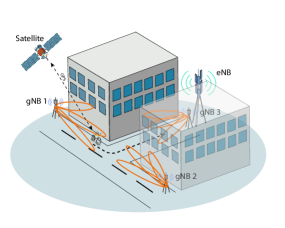
Figure 1: Overview of the scenario: a UE uses GPS context information and dual connectivity to improve handover latency in an urban scenario.

Typically, an RL agent optimizes its action based on a customized reward or objective function. The design of a reward function will intend to maximize or minimize certain metric of interest. In addition, a reward function could also be used in scenarios where our agent’s goal is known. However, in goal-directed problems as in the majority of RL problems, sparse rewards are a significant challenge that affects the learning of robust value functions and thus, optimal action selection. Hierarchical reinforcement learning (hRL) [4] helps to solve the aforementioned problem by splitting the value function into two levels: a meta-controller and a controller.

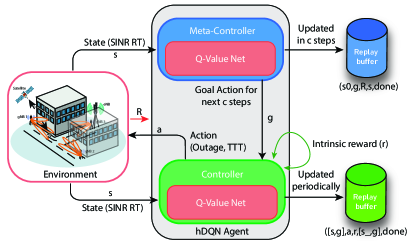
Figure 2: Hierarchical Deep Q-Learning (HiDQL) applied in a Multiple Radio Access Technology (multi-RAT) LTE-NR scenario. The HiDQL agent located in the coordinator will optimize TTT and SINR outage metrics to reduce multi-RAT handover latency.

In this paper, we address the handover problem in an LTE-NR network with dual connectivity using a hierarchical and a non-hierarchical architecture. Additionally, we consider the context information to further improve the DC algorithm performance. To do so, we use a novel hierarchical Deep Q-learning algorithm named hierarchical Deep Q-Learning (HiDQL) and a non-hierarchical RL approached named Clipped Double Q-Learning (CDQL) to improve handover latency in a DC architecture. HiDQL presents an architecture comprised by a meta-controller and a controller. Two parameters are adjusted in this problem: Threshold to Time (TTT) and signal-to-interference-plus noise ratio (SINR) outage. TTT is defined as the time to hold the condition of triggering the handover algorithm named Secondary Cell Handover (SCH), discussed in section III. On the other hand, SINR outage is defined as the SINR threshold in which we consider a cell being in outage from the User Equipment (UE). The controller will propose actions in terms of TTT and SINR outage aided by the proposed goals by the meta-controller in order to minimize handover latency. We compare our results with an algorithm presented in [5] named Clipped Double Q-Learning (CDQL) that proved its efficiency in load balancing problems. Our results show an improvement in terms of latency with a gain of 47.6% and 26.1% for Digital-Analog beamforming (BF), 17.1% and 21.6% for Hybrid-Analog BF, and 24.7% and 39% for Analog-Analog BF when comparing the RL-schemes with the baseline’s best results. Additionally, we observed faster convergence when utilizing the CDQL algorithm, meanwhile the HiDQL showed improved results in terms of handover latency. Finally, we obtained an improvement regarding handover latency under line of sight assumptions when considering context information in comparison with no context available.

The rest of this paper is organized as follows. Section II presents the existing works related to dual connectivity and hierarchical algorithms applications in wireless networks. System model is demonstrated in Section III. Section IV provides a description of the Markov Decision process of the RL algorithms and baselines utilized. Section V depicts the performance evaluation and comparison with the baseline solutions. Section VI introduces context information in the DC architecture and its performance evaluation. Finally, section VII concludes the paper.

II Related work

To the best of our knowledge, there is no previous work where hRL has been utilized to optimize handover key parameters such as TTT and SINR cell outage in a 5G dual connectivity scenario. The aforementioned parameters are defined in detail in section V. However, dual connectivity (DC) has been studied thoroughly in the literature. These studies are summarized below.

In [6], the authors give an overview of the 4G LTE-NR DC based on the new specifications given by 3GPP. A study case showed that DC is capable of providing coverage and capacity improvements when compared to standalone LTE-NR deployed individually. More recently, in [7] the authors perform an analysis of the dual connectivity proposal in the 3GPP release 15[2]. In addition to the existent specification, the authors remarked the possibilities to include a Secondary Cell controller to manage the multi-radio DC signaling. Furthermore, in [8], the authors present a survey on recent developments of 4G/5G DC, as well 4G/5G internetworking performance and future research challenges and open issues.

Besides, the body of works in DC, the concept of hRL has not been explored much in the the wireless community. In [9], the authors study outage avoidance in a two-hop cooperative relay network by utilizing hRL in optimizing relay selection and both source and relays transmission power. In [10], the authors propose a hierarchical deep Q-network to perform dynamic multi-channel spectrum sensing in cognitive networks. In this work the actions corresponds to the selection of channel and the reward corresponds to the channel status (busy/idle). In the following sections, we will introduce the dual connectivity architecture utilized in this work and explain how RL emerges as effective solution in the optimization of the handover in DC scenarios. Additionally, we forsee the advantage of embedding context-awareness in the DC architecture.

III System model

In this work, we use a DC architecture presented in [11] inspired by a 3GPP’s previous DC proposal [1]. In [11], the authors leverage the usage of a DC framework to improve, among others, handover latency by using an algorithm named Secondary Cell Handover (SCH). SCH enables fast switching between the LTE and 5G RATs and is managed by a defined entity named coordinator. In this architecture the eNB takes the role of coordinator and controls the multi-RAT switch. Two main parameters are controlled by the coordinator: TTT and SINR cell outage. As part of the SCH algorithm, the coordinator will trigger the SCH when any of the RATs involved report a better SINR and neither of the RATs are in outage. Additionally, it will check the condition to trigger the SCH algorithm for TTT seconds to avoid ping pong scenarios. This algorithm resembles the classical LTE and 5G handover with the exception that no initial access is necessary and no interaction with the MME is required thanks to the nature of the DC architecture. As mentioned, the handover will be triggered based on SINR and specifically using a table named the Complete Report Table (CRT) comprised by the UE’s SINR report tables from each gNodeB (gNB). Each gNB will perform a sweep over a number of predefined directions and will sense the Sounding Reference Signals from the UE’s to obtain SINR measurements. The collected data will be sent via X2 interface to the coordinator. The delay incurred to perform the measurements sweeps is directly related with the beamforming (BF) technology used by the UEs and gNBs. The aforementioned delay, $D$, is calculated as:

$$D=\frac{N_{gNB}N_{UE}T_{per}}{L},$$ (1)

where $N_{gNB}$ and $N_{UE}$ correspond to the number of required sweep directions needed for measurement collection by the gNBs and UEs, respectively. $T_{per}$ is the SRS periodicity and $L$ corresponds to the BF capabilities that will present different values if the transceiver is fully digital or analog. The relationship between $D$ and $L$ can be calculated using typical values as depicted in Table I (Modified from [11]).

TABLE I: Relationship between $L$ and $D$

gNB-UE BF	$L$ (gNB/UE)	$D$* (ms)
Analog-Analog	$1/1$	25.6
Hybrid-Analog	$2/1$	16.8
Digital-Analog	$N_{gNB}/1$	1.6

• D in Eq. 1 is calculated with $T_{per}=200\mu{s}$, $N_{gNB}=16$ and $N_{UE}=8$

In this paper, we consider an LTE-NR network with dual connectivity and consisting of $M_{T}$ gNBs. Additionally, an eNB will act as a coordinator and thus, serving the $M_{T}$ gNBs. A mobile user is dual connected to one gNB and one eNB at the same time. We consider an urban scenario with two buildings as shown in Fig. 1. The channel considered for the eNB is the 3GPP Channel Model, meanwhile the 3GPP building channel type and losses based on the 3GPP UMi Street Canyon propagation model is used for the gNBs.

IV Hierarchical Deep Q-Learning (HiDQL)

In this work, we use a state-of-the-art hierarchical Deep Q-learning (HiDQL) algorithm. This algorithm is presented in [4], where the goal-directed behavior is studied under some specific sparse reward problems such as the Montezuma Revenge and a complex discrete stochastic decision process.

As shown in figure 2, a hierarchical agent located in the coordinator observes the user’s SINR report table and receives the extrinsic reward based on the feedback from the environment in terms of handover latency. This agent will adjust key parameters as TTT and SINR outage in order to maximize the agent’s extrinsic reward. In the following subsection, we will present an overview of HiDQL and then formally define our solution.

1

2

3Initialize $c_{max}$, $\kappa$, experience replay buffers $\{B_{mc}$, $B_{c}\}$, policy networks $\{\mu_{mc}$, $\mu_{c}\}$, for the meta-controller and controller, respectively.

4 Function Done($c$, $c_{max}$, $\mathcal{S}_{\kappa}$, $\kappa$ ):

5      

6      if ($c=c_{max}$ or $\mathcal{S}_{\kappa}<\kappa$) then

7            return True

8      else

9            return False

10       end if

11      

12

13End Function

14for environment step $t\leftarrow 1$ to $T$ do

15       $c\leftarrow 0$

16       Init environment and initial state

17       Execute goal from meta-controller: $g=\mu_{mc}(s)$

18       while c_max not reached do

19             $R\leftarrow 0$; $s_{0}\leftarrow s$; $\mathcal{S}_{\kappa}$ = false

20            

21            while not Done  do

22                   Execute action from controller: $a=\mu_{c}(s,g)$

23                   Get next state $s^{\prime}$ and similarity condition $\mathcal{S}_{\kappa}$ ;

24                   Calculate intrinsic reward $r$ and receive extrinsic reward $r_{g}$;

25                   Store $([s,g],a,r,[s^{\prime},g],{\texttt{Done}})$ in replay buffer $B_{c}$;

26                   Update $\mu_{c}$;

27                   $c:=c+1$; $R:=R+r_{g}$; $s:=s^{\prime}$

28                  

29             end while

30            Store $(s_{0},g,R,s,{\texttt{Done}})$ in replay buffer $B_{c}$;

31             Update $\mu_{mc}$;

32             if not Done then

33                   Execute goal from meta-controller: $g=\mu_{mc}(s)$

34             end if

35            

36       end while

37      

38 end for

Algorithm 1 Hierarchical Deep Q-Learning (HiDQL)

IV-A Meta-controller and controller action space selection

In the proposed hierarchical approach described in Algorithm 1, the meta-controller proposes goals or high level actions when the maximum $c$ steps, $c_{max}$ is achieved or when the similarity between the goal and low-level action, $\mathcal{S}_{\kappa}$ falls under a predefined threshold index $\kappa$ as defined in the function Done. Meanwhile, the controller’s low level actions are executed $c$ inner steps. For both levels, the actions are defined in the same fashion as:

$$A(t)=\begin{bmatrix}a_{out}(t),a_{ttt}(t)\end{bmatrix},$$ (2)

where $a_{out}$ and $a_{ttt}$ are the SINR outage and TTT values, respectively. Such values are discretized into $K_{o}$ and $K_{TTT}$ levels according the maximum and minimum defined values. The possible values for $a_{out}$ and $a_{ttt}$ are defined as:

$$A_{out}=\{O_{min},O_{min}+\frac{O_{max}-O_{min}}{K_{o}-1},...,O_{max}\},$$ (3)

$$A_{ttt}=\{TTT_{min}, TTT_{min}+$$ (4)

$$\frac{TTT_{max}-TTT_{min}}{K_{TTT}-1},\cdots,TTT_{max}\},$$

where $O_{min}$, $O_{max}$ and $TTT_{min}$, $TTT_{max}$ are predefined maximum and minimum values of SINR outage and TTT values, respectively. Finally, the size of the meta-controller and controller action spaces become $S=|A_{out}|*|A_{ttt}|$.

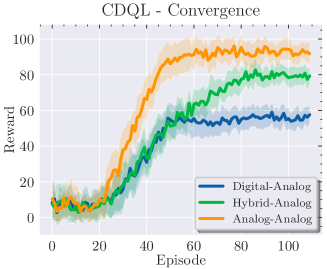
(a)

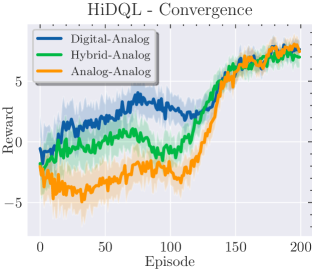
(b)

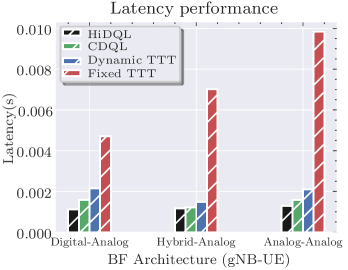
(c)

Figure 3: (a) CDQL convergence performance. (b) HiDQL convergence performance. contain. (c) Latency performance of the baselines Dynamic TTT and Fixed TTT and the proposed RL schemes CDQL and HiDQL.

IV-B State space selection

The state space is comprised by the Complete Report Table (CRT), which contains the relationship in terms of SINR of each user and the perceived gNB SINR. The SINR between an $i^{th}$ gNB and $n^{th}$ UE is calculated as follows:

$$SINR_{i,n}=\frac{\frac{P_{TX}}{PL_{i,n}}G_{i,n}}{\sum_{k\neq i}\frac{P_{TX}}{PL_{k,n}}G_{k,n}+W_{tot}\times N_{0}},$$ (5)

where $G_{i,n}$ and $PL_{i,n}$ are the beamforming gain and the pathlosss obtained between $i^{th}$ gNB and $n^{th}$ UE. $P_{TX}$ is the transmit power and $W_{tot}\times N_{0}$ is the thermal noise power. Thus, the state space is defined as follows:

$$S(t)=\begin{bmatrix}C(t)\end{bmatrix},$$ (6)

where $C(t)$ corresponds to the CRT with a size of $|C(t)|=M_{T}$.

IV-C Intrinsic and extrinsic reward

The intrinsic reward function is calculated by the controller by taking into account the goal selected by the meta-controller in $c$ inner steps. Such a reward is defined as:

$$r(t)=r_{i}(t)+r_{l^{2}}(t),$$ (7)

where $r_{i}$ corresponds to the immediate reward obtained from the environment and $r_{l^{2}}$ corresponds to reward based on the $l^{2}$-norm between the controller’s action and the meta-controller’s goal. Such rewards are defined as follows:

$$r_{i}(t)=\begin{cases}-f_{-1}(-D_{avg}^{u})&\text{if }D_{avg}^{u}<D_{tol}^{BF},\\ 0&\textit{otherwise}\end{cases}$$ (8)

where $f_{-1}(\cdot):[-e^{-1},0)\rightarrow[-1,-\infty)$ is the lower branch of the Lambert function $y=f_{-1}(ye^{y})$ [12]. $D_{tol}^{BF}$ is the maximum tolerable delay corresponding to the value of the best latency results per BF technology in the non-RL approaches. $D_{avg}^{u}$ is the average latency of the UE. Additionally, we scale linearly $D_{avg}^{u}\rightarrow[e^{-1},0]$.

$$r_{l^{2}}(t)=\begin{cases}1&\text{if $\mathcal{S}_{\kappa}<\kappa$,}\\ -1&\textit{otherwise},\end{cases}$$ (9)

where $\mathcal{S}_{\kappa}=|a-g|_{2}$ and $\kappa$ is the similarity threshold between the action and goal. Finally, we can express the extrinsic reward as:

$$R=\sum_{j=t-c}^{c}r(j),$$ (10)

where the extrinsic reward is defined as the sum of the intrinsic reward during the c inner steps.

IV-D Clipped Double Q-Learning: RL scheme

In addition to HiDQL, we utilized an RL solution named Clipped Double Q-Leaning (CDQL) [5]. For the CDQL algorithm, the state and action space correspond to the ones used in the lower level by the HiDQL algorithm in (6) and (2), respectively, meanwhile the reward corresponds to the intrinsic reward defined in (8).

IV-E Baselines: Fixed TTT and Dynamic TTT

For the present work, as baselines, we take a fixed and a dynamic solution into consideration. The fixed and dynamic solutions were proposed in [11], where the fixed solution has a fixed value of TTT and in the dynamic solution TTT is calculated as follows:

$$\emph{f}_{TTT}(\bm{\Delta})=TTT_{max}-\frac{\bm{\Delta}-\bm{\Delta}_{min}}{\bm{\Delta}_{max}-\bm{\Delta}_{min}}(TTT_{max}-TTT_{min}),$$ (11)

where $\bm{\Delta}$ corresponds to the difference between the serving cell and the best gNB in terms of SINR.

V Performance Evaluation

V-A Simulation Setting

We implement our proposed solution using the discrete network simulator ns-3 and its module mmWave [13]. Additionally, ns3-ai module [14] is used to interface the simulation environment to our RL algorithm written in Python 3.9. Simulation settings and RL parameters are depicted in Table II and Table III, respectively.

TABLE II: Network settings

Parameter	Value
$M_{T}$	3
Number of UEs	1
gNB center frequency	28 GHz
gNB system bandwidth	200 MHz
gNB numerology	2
gNB Pathloss Model	3GPP Umi-Street Canyon
gNB Channel condition model	Buildings
gNB antenna height	10 m
gNB number of antennas	64
eNB Center Frequency	2 GHz
eNB System Bandwidth	100 MHz
eNB Pathloss Model	3GPP
Max Tx power	30 dBm
UE number of antennas	16
UE antenna height	1.6 m
UE speed	13 m/s
UE Tx power	10 dBm
Traffic Model	On-Off UDP application
	Packet payload size = 512 Bytes
	Packet window size = 256
	Interval = 20 $\mu$s

TABLE III: Learning parameters

Parameter	Value
Handover algorithm	Threshold to time: $TTT_{max}=150$ ms; $TTT_{min}=25$ ms
	SINR Outage: $O_{max}=-3$ dBm; $O_{min}=-8$ dBm
	$D_{tol}^{BF}$ = $min(D_{f}^{BF},D_{d}^{BF})$ *
Gym environment step time	Event-based
Batch size	32
	Number of hidden layers ($N_{h}$) : 2
	Number of neurons/layer ($n_{l}$) : 64
HiDQL	$\kappa=0.25$
	Optimizer : Meta-Controller: Adam (1e-4),
	Controller: Adam (1e-4)
$c_{max}$	50 steps
CDQL	Update target model type : Polyak averaging
	$\gamma=0.95,\epsilon=1.0,\epsilon_{min}=0.001,\epsilon_{decay}=0.995$
	Optimizer : Adam (1e-4)

• *$D_{f}^{BF}$ and $D_{d}^{BF}$ correspond to the latency performance per BF technology of the fixed TTT and dynamic TTT
  solutions, respectively.

V-B Simulation Results

We present the performance results of our proposed scheme in terms of convergence and handover latency. Figure 3 (a), (b) depicts the convergence behavior for the CDQL and HiDQL algorithms for different BF mechanisms, respectively. It can be observed that CDQL presents a faster convergence when compared with HiDQL. However, converged reward values are not achieved equally among the tested BF architectures. HiDQL presents a slower convergence time than CDQL however with a similar maximum convergence reward value among BF methods. The intuition behind the previous results correspond to the inner nature of hierarchical learning. HiDQL performs an iterative search through the meta-controller’s proposal of goals to the controller and thus, obtaining optimum action selection in challenging scenarios as described in [4]. The difference between reward scales between HiDQL and CDQL corresponds to how the reward is defined in both algorithms, thus a comparison in terms of the value of the reward is not relevant.

TABLE IV: RL vs non-RL latency comparison

	Latency improvement (%)
	Digital-Analog BF		Hybrid-Analog BF		Analog-Analog BF
RL Scheme	F-TTT	D-TTT	F-TTT	D-TTT	F-TTT	D-TTT
HiDQL	76.1	47.6	83.5	21.6	87.0	39.0
CDQL	66.2	26.1	82.5	17.1	83.8	24.7

In Fig. 3 (c), we present the latency performance of our techniques and the baselines: fixed TTT (F-TTT), dynamic TTT (D-TTT). From the two baselines, the best performance in terms of latency is achieved by the dynamic TTT parameter selection. On the other hand, we obtained an average 9% improvement when comparing HiDQL and CDQL in terms of latency results. However, based on more detailed look into results, we further focus in Table IV on the latency results improvements over the previous solutions F-TTT and D-TTT.

As shown in Table IV, when compared with the dynamic TTT results, a gain of 47.6% and 26.1%, for Digital-Analog BF, 17.1% and 21.6%, for Hybrid-Analog BF, and 24.7% and 39% for Analog-Analog BF were obtained for HiDQL and CDQL, respectively.

TABLE V: CI vs. non-CI latency comparison

	Latency improvement (%)
	Digital-Analog BF	Hybrid-Analog BF	Analog-Analog BF
CI	Non-CI
F-TTT	74.9	2.57	28.5
D-TTT	40.1	8.7	29.7

VI Context information aware DC handover

In addition to the SCH algorithm used as part of the proposed DC architecture, we foresee the possible advantages of using context information to improve handover time. In [15], the authors give an overview of the typical initial access (IA) cell search algorithms where contrary to LTE, 5G NR provide mechanisms to determine suitable initial directions of transmission to avoid high isotropic losses. Among the IA algorithms, context information (CI)-based algorithms allow users to be aware of the location of the surrounded 5G NR antennas through an LTE link and GPS. In this work, we leverage GPS information as context and reduce the sector in which a gNB should sense the space towards an UE. Figure 4 depicts the beforementioned mechanism, where given the user position $P1$ the gNB is able to calculate a reduced sector to obtain the periodic SRS signals from the surrounded UEs. We also assume that each UE has line of sight both with the coordinator and the gNBs. The proposed mechanism is described in Algorithm 2. As shown in Table V, context awareness directly improves the DC handover mechanism with a considerable latency improvement.

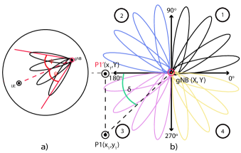
Figure 4: a) $\pm\psi$ indicates the sweep angle to obtain SINR measurements. b) $\delta$ corresponds to the relative angle used to derive the sweep sector angle.

1 Result: Sector’s angle to perform measurements sweeps.

2 Given P1$(x_{1},y_{1})$ and $(X,Y)$, the UE’s and gNB geolocations, respectively.

3 Additionally, $\delta=\arcsin\frac{\vec{d_{2}}}{\vec{d_{1}}}$ and $\Theta^{gNB}=\frac{2\pi}{N}$; where $\vec{d_{2}}=\overrightarrow{{P_{1}P_{1}^{\prime}}}$ and $\vec{d_{1}}=\overrightarrow{{P_{1}{gNB}}}$

4 # Step 1: Detect UE’s relative quadrant $q\in\{1,2,3,4\}$. Calculate angle $\phi$ respect gNB quadrant one.

5 if $y_{1}>Y$ and $x_{1}>X$ then

6       # UE in $1^{st}$ quadrant

7       $\phi=\delta$

8 else if $y_{1}>Y$ and $x_{1}<X$ then

9       # UE in $2^{nd}$ quadrant;

10       $\phi=\frac{\pi}{2}+\delta$

11 else if $y_{1}<Y$ and $x_{1}<X$ then

12       # UE in $3^{rd}$ quadrant;

13       $\phi=\pi+\delta$

14 else

15       # UE in $4^{th}$ quadrant;

16       $\phi=\frac{3\pi}{2}+\delta$

17 end if

18# Step 2: Calculate sector angle ($S_{A}$)

19 $S_{A}\in[\phi-2\Theta,\phi+2\Theta]$

Algorithm 2 CI-aware sector sweep selection algorithm

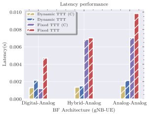
Figure 5: Context information (C) latency performance results when utilizing Dynamic TTT and Fixed TTT baselines.

VII Conclusions

In this paper, we presented two Reinforcement Learning (RL)-based dual connectivity (DC) solutions that further improve latency metric in inter-RAT handover. Additionally, we propose leveraging an initial access cell search algorithm that utilizes context information to reduce the latency in gNB-UE’s measurement collection. We compared two RL solutions named Hierarchical Deep Q-Learning (HiDQL) and Clipped Double Q-Learning (CDQL) with two previously proposed baselines, fixed Threshold to Time (TTT) and dynamic TTT, obtaining a significant gain in both cases in terms of latency with a 47.6% and 26.1%, for Digital-Analog BF, 17.1% and 21.6%, for Hybrid-Analog BF and 24.7% and 39% for Analog-Analog BF when compared with the baselines’ best results. Finally, we presented a context-aware mechanism under line of sight assumptions and obtained a significant improvement in terms of latency when compared with the case of no context. As future work we forsee the integration of the presented context-aware mechanism and reinforcement learning to further improve the DC handover mechanism.

VIII Acknowledgment

This research is supported by Mitacs and Ericsson.

References

- [1] 3GPP TR 36.842, “Study on small cell enhancements for E-UTRA and E-UTRAN, v12.0.0 ,” Tech. Rep., 2013.
- [2] 3GPP TS 37.340, “Universal Mobile Telecommunications System (UMTS), LTE, 5G, NR, Multi-connectivity, Overall description, Stage-2,” Tech. Rep., 2019.
- [3] M. Elsayed and M. Erol-Kantarci, “AI-Enabled Future Wireless Networks: Challenges, Opportunities, and Open Issues,” IEEE Veh. Technol. Mag., 2019.
- [4] T. D. Kulkarni, K. R. Narasimhan, A. Saeedi, and J. B. Tenenbaum, “Hierarchical deep reinforcement learning: Integrating temporal abstraction and intrinsic motivation,” in Advances in Neural Information Processing Systems (NeurIPS), 2016.
- [5] P. E. Iturria-Rivera and M. Erol-Kantarci, “QoS-Aware Load Balancing in Wireless Networks using Clipped Double Q-Learning,” in 2021 IEEE 18th International Conference on Mobile Ad Hoc and Smart Systems (MASS), 2021.
- [6] O. N. C. Yilmaz, O. Teyeb, and A. Orsino, “Overview of LTE-NR Dual Connectivity,” IEEE Commun. Mag., vol. 57, no. 6, pp. 138–144, 2019.
- [7] J. F. Monserrat, F. Bouchmal, D. Martin-Sacristan, and O. Carrasco, “Multi-Radio Dual Connectivity for 5G Small Cells Interworking,” IEEE Commun. Stand. Mag., vol. 4, pp. 30–36, 2020.
- [8] M. Agiwal, H. Kwon, S. Park, and H. Jin, “A Survey on 4G-5G Dual Connectivity: Road to 5G Implementation,” IEEE Access, vol. 9, pp. 16 193–16 210, 2021.
- [9] Y. Geng, E. Liu, R. Wang, and Y. Liu, “Hierarchical Reinforcement Learning for Relay Selection and Power Optimization in Two-Hop Cooperative Relay Network,” IEEE Trans. Commun., vol. 70, pp. 171–184, 2021.
- [10] S. Liu, J. Wu, and J. He, “Dynamic multichannel sensing in cognitive radio: Hierarchical reinforcement learning,” IEEE Access, vol. 9, pp. 25 473–25 481, 2021.
- [11] M. Polese, M. Giordani, M. Mezzavilla, S. Rangan, and M. Zorzi, “Improved Handover Through Dual Connectivity in 5G mmWave Mobile Networks,” IEEE J. Sel. Areas Commun., vol. 35, no. 9, pp. 2069–2084, 2017.
- [12] R. M. Corless, G. H. Gonnet, D. E. Hare, D. J. Jeffrey, and D. E. Knuth, “On the Lambert W function,” Adv. Comput. Math., no. 5, p. 329–359, 1996.
- [13] M. Mezzavilla, M. Zhang, M. Polese, R. Ford, S. Dutta, S. Rangan, and M. Zorzi, “End-to-End Simulation of 5G mmWave Networks,” IEEE Commun. Surveys Tuts., vol. 20, no. 3, pp. 2237–2263, 2018.
- [14] H. Yin, P. Liu, K. Liu, L. Cao, L. Zhang, Y. Gao, and X. Hei, “Ns3-Ai: Fostering Artificial Intelligence Algorithms for Networking Research,” in WNS3 2020: Proceedings of the 2020 Workshop on ns-3, 2020.
- [15] M. Giordani, M. Mezzavilla, and M. Zorzi, “Initial Access in 5G mmWave Cellular Networks,” IEEE Commun. Mag., vol. 54, no. 11, pp. 40–47, 2016.