and () two-particle femtoscopic correlations in PbPb collisions at $\sqrtsNN=5.02\TeV$

Abstract

Two-particle correlations are presented for , , and strange hadrons as a function of relative momentum in lead-lead collisions at a nucleon-nucleon center-of-mass energy of 5.02. The dataset corresponds to an integrated luminosity of 0.607and was collected using the CMS detector at the CERN LHC. These correlations are sensitive to quantum statistics and to final-state interactions between the particles. The source size extracted from the $\PKzS\PKzS$ correlations is found to decrease from 4 to 1fm in going from central to peripheral collisions. Strong interaction scattering parameters (, scattering length and effective range) are determined from the $\PGL\PKzS$ and $\PGL\PGL$ (including their charge conjugates) correlations using the Lednický–Lyuboshitz model and are compared to theoretical and other experimental results.

0.1 Introduction

Two-particle correlations in relative momentum, so-called femtoscopic correlations, arising from relativistic heavy ion collisions provide a powerful tool for studying both the quark-gluon plasma (QGP) that is created in the collisions, and the subsequent interactions of the emitted particles [1]. All two-particle correlations are affected by final-state interaction (FSI) effects, and correlations of identical particles are also sensitive to the constraints of quantum statistics (QS). The correlations among the neutral , , and particles, collectively referred to as $\textrm{V}^{0}$ particles, are of special interest. First, they can be used to determine the space-time extent of the QGP. In addition, information can be extracted about the strong-interaction scattering parameters, , the scattering length and the effective range, that is impossible to obtain from currently achievable scattering experiments [2, 3, 4, 5, 6]. Because of their relatively heavy mass and the absence of a Coulomb interaction, femtoscopy based on particles supplements the more commonly studied pion and charged kaon pairs [7]. The results from $\PGL\PGL$ correlation studies can help constrain baryon-baryon and, more specifically, hyperon-hyperon interaction models that are used, for example, in modeling the composition of neutron stars [8, 9, 10].

Regarding the scattering parameters, of particular interest is establishing whether the interaction between two particles allows for the existence of the H-dibaryon, a bound state with quantum numbers $I=0$, $J^{P}=0^{+}$, $S=-2$. In 1977, R. L. Jaffe predicted the existence of such a six-quark ($\PQu\PQu\PQd\PQd\PQs\PQs$) state having a mass about 81below the threshold of twice the mass by considering the strong attraction resulting from color magnetic interactions [11]. Although a double hypernucleus, ${}^{\;\;\;\;6}_{\PGL\PGL}{\mathrm{He}}$, was subsequently observed in the NAGARA event from the E313 hybrid emulsion experiment at KEK [12, 13], the observed $\PGL\PGL$ binding energy was not consistent with the conjectured H-dibaryon [14]. A study of $\PGL\PGL$ correlations may provide additional information on whether the baryon-baryon interaction can lead to the formation of the conjectured H-dibaryon.

Recently, the ALICE Collaboration reported on $\PGL\PK$ correlations in lead-lead (PbPb) collisions at a center-of-mass energy per nucleon pair of $\sqrtsNN=2.76\TeV$ [15]. According to their findings, the strong force is repulsive in $\PGL\PKp$ interactions, yet attractive in $\PGL\PKm$ interactions. For the $\PGL\PKzS$ pairs, the uncertainty of the ALICE results does not permit a definite conclusion on whether the associated strong interaction is repulsive or attractive. A more precise measurement of $\PGL\PKzS$ correlations should improve our understanding of the strong interaction in baryon-meson systems.

This Letter presents $\PKzS\PKzS$, $\PGL\PKzS$, and $\PGL\PGL$ femtoscopic correlations as a function of relative momentum in PbPb collisions at $\sqrtsNN=5.02\TeV$, using data recorded by the CMS experiment during the 2018 LHC run. The $\PKzS\PKzS$ correlations are measured in six centrality intervals within the 0–60% range, where centrality refers to the percentage of the total inelastic hadronic nucleus-nucleus cross section [16], and 0% corresponds to the maximum overlap of the colliding nuclei. The $\PKzS\PKzS$, $\PGL\PKzS$, and $\PGL\PGL$ correlations are measured in an integrated centrality range (0–80%), with the $\PGL\PGL$ femtoscopic correlation measured in PbPb collisions at the LHC for the first time. The source size and strong interaction parameters are determined using the Lednický–Lyuboshitz (LL) model [17]. Unless otherwise indicated, all measurements include the charge conjugate states, so $\PGL\PKzS$ and $\PGL\PGL$ include $\PAGL\PKzS$ and $\PAGL\PAGL$, respectively. Tabulated results are provided in the HEPData record for this analysis [18].

0.2 Experimental setup and data sample

The central feature of the CMS apparatus is a superconducting solenoid of 6m internal diameter, providing a magnetic field of 3.8T. Within the solenoid volume there is a silicon pixel and strip tracker, a lead tungstate crystal electromagnetic calorimeter, and a brass and scintillator hadron calorimeter, each composed of a barrel and two endcap sections. The silicon pixel detector [19] is composed of 1856 silicon pixel modules distributed in four 54 cm long barrel layers at radii of 2.9–16.0cm plus three pairs of endcap disks covering radii of 4.5–16.1cm at longitudinal distances of 31–51cm from the origin. The 15 148 silicon strip module are arranged in 10 barrel layers at radii of 20–116cm plus 3 pairs of small and 9 pairs of large endcap disk layers. Charged particles of pseudorapidity $\abs{\eta}<3$ are reconstructed with the combined system. For particles with transverse momentum of $1<\pt<10\GeV$, the track resolutions are typically 1.5% in and 20–75$\mum$ in the transverse impact parameter [20]. The barrel and endcap detectors are extended to the forward region with two calorimeters which use steel as the absorber and quartz fibers as the sensitive material. These hadron forward (HF) calorimeters are located 11.2m from the interaction region, one on each side, and provide coverage in the range $3.0<\abs{\eta}<5.2$. These detectors are segmented into multiple $0.175{\times}0.175$ ($\Delta\eta{\times}\Delta\phi$) “towers”, where $\phi$ is azimuthal angle in radians. Muons are measured in gas-ionization detectors embedded in the steel flux-return yoke outside the solenoid. Events of interest are selected using a two-tiered trigger system. The first level, composed of custom hardware processors, uses information from the calorimeters and muon detectors to select events at a rate of around 100kHz within a fixed latency of about 4 [21]. The second level, known as the high-level trigger, consists of a farm of processors running a version of the full event reconstruction software optimized for fast processing, and reduces the event rate to around 1kHz before data storage [22]. A more detailed description of the CMS detector, together with a definition of the coordinate system used and the relevant kinematic variables, can be found in Ref. [23].

With an integrated luminosity of 0.607 [24, 25], this analysis uses $4.27\times 10^{9}$ minimum bias events that are triggered by requiring signals above the readout threshold of 3in each of the HF calorimeters [22]. Background events due to beam-gas interactions and non-hadronic collisions are filtered offline by applying the procedure described in Ref. [26]. The events used in this analysis are required to have at least one primary interaction vertex determined using two or more tracks [27] within a distance of 15cm from the center of the nominal interaction point along the beam axis and to have at least two calorimeter towers in each HF detector with energy deposits of more than 4per tower. The shapes of the clusters in the pixel detector are required to be compatible with those expected in PbPb collisions in order to suppress the contamination from events with multiple collisions [28]. The combined trigger and offline selection efficiency for inelastic events is greater than 95%. The event centrality is obtained from the transverse energy deposited in both HF calorimeters, using the methodology described in Ref. [29]. The analysis makes use of a minimum bias Monte Carlo PbPb sample, based on the 1.9 [30] event generator with a full detector simulation using  [31].

0.3 Reconstruction of and candidates

The and candidates, denoted as $\textrm{V}^{0}$ candidates, used in this study are reconstructed as in previous CMS analyses [32, 33, 34]. The $\textrm{V}^{0}$ candidates are found by combining oppositely charged tracks that pass criteria based on the “loose” selection discussed in Ref. [27]. The charged tracks are assumed to be $\PGpp\PGpm$ in reconstruction and $\PGpm\Pp$ in reconstruction. For the latter, the higher momentum track is assumed to be a proton since the proton carries nearly all of the momentum in the decay. Each of the oppositely charged tracks must have hits in at least three layers of the silicon tracker, and both tracks must have transverse and longitudinal impact parameter significances (defined as the parameter value divided by its uncertainty) with respect to the primary vertex greater than 1. The two tracks are fitted to a common vertex and the $\chi^{2}$ per degree of freedom (dof) from the fit must be less than 7. The distance of closest approach between the two tracks is required to be less than 1cm. As a consequence of the long lifetime of and particles, the significance of the $\textrm{V}^{0}$ decay length, which is the three-dimensional distance between the primary and $\textrm{V}^{0}$ vertices divided by its uncertainty, is required to be greater than 2.5 to reduce combinatorial background contributions. To remove candidates misidentified as particles and vice versa, the () candidates must have a corresponding $\PGp\PGp\;(\Pp\PGp)$ mass more than 14 (7)(corresponding to approximately 3 times the average resolution) away from the world-average value [35] of the () mass. The angle $\theta$ between the $\textrm{V}^{0}$ momentum vector and the vector connecting the primary and $\textrm{V}^{0}$ vertices is required to satisfy $\cos\theta>0.999$. This reduces the contribution from nuclear interactions, random combinations of tracks, and particles originating from weak decays of and particles.

Further selection of $\textrm{V}^{0}$ candidates is performed with a boosted decision tree (BDT) [36]. The selection is optimized separately for and candidates. The discriminating variables include: the collision centrality, the $\textrm{V}^{0}$ candidate and rapidity ($y$), the distance of closest approach of the track pair, the three-dimensional decay length and significance, $\cos\theta$, and the $\textrm{V}^{0}$ vertex fit $\chi^{2}$. The included variables related to the $\textrm{V}^{0}$ daughters are , uncertainty in , $\eta$, the number of hits in the silicon tracker, the number of pixel detector layers with hits, and the transverse and longitudinal impact parameter significances with respect to the primary vertex. The BDT training is performed using the simulated minimum bias sample separated into the signal and background subsamples using the generator-level information. The mesons are selected with $1<\pt<8.5\GeV$ and $\abs{y}<1$, while the baryons are required to have $1.8<\pt<8.5\GeV$ and $\abs{y}<1$. The minimum and maximum $y$ requirements are used to reduce background while the maximum requirement is to reduce contributions from jets. The combined $\textrm{V}^{0}$ reconstruction and selection efficiencies are strongly dependent on the centrality of the event and the of the $\textrm{V}^{0}$. Integrating over the selected ranges, the combined efficiencies from the most central to peripheral PbPb collisions are 1–3% for and 1–2% for . The $\textrm{V}^{0}$ reconstruction algorithm does not prevent a track from being used for more than one $\textrm{V}^{0}$. While this is normally an infrequent occurrence, selecting pairs of $\textrm{V}^{0}$ particles close together in phase space makes it a significant contribution. To resolve this problem, for each correlation measurement, a check of each pair of $\textrm{V}^{0}$ candidates is performed and if two $\textrm{V}^{0}$ candidates are found to share one or both daughter tracks, one of the $\textrm{V}^{0}$ candidates is randomly selected to be removed from the event.

Fits to the invariant mass spectrum are performed using a sum of three Gaussian functions with a common mean to describe the signal distribution and a fourth-order polynomial to describe the background. These empirical functions were chosen to provide a good description of the data. Peak and sideband invariant mass regions are defined to select events dominated by signal and background, respectively. Defining $\sigma$ as the average resolution based on the Gaussian sum, the peak regions are selected to be within ${\pm}2\sigma$ from the nominal $\textrm{V}^{0}$ mass and are given by $486<\mathrm{M(\PGpp\PGpm)}<509\MeV$ and $1111.5<\mathrm{M(\Pp\PGpm)}<1120.4\MeV$ for and candidates, respectively. The sideband regions are selected to be more than $4\sigma$ from the nominal $\textrm{V}^{0}$ mass and are given by $23.5<\abs{\mathrm{M(\PGpp\PGpm)}-497.5}<62.5\MeV$ for candidates and $1080<\mathrm{M(\Pp\PGpm)}<1107.5\MeV$ together with $1124.2<\mathrm{M(\Pp\PGpm)}<1160\MeV$ for candidates. Examples of invariant mass distributions for $\PGpp\PGpm$ and $\Pp\PGpm$ pairs, and their corresponding fits in the 0–80% centrality range, are shown in Fig. 1.

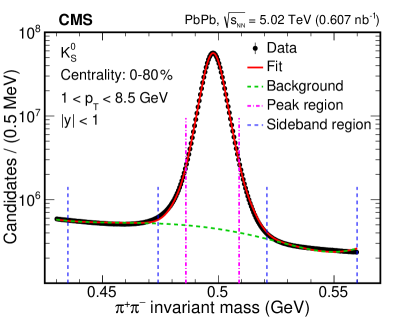
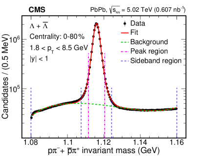
Figure 1: The invariant mass of (left) and (right), and their corresponding fits in the 0–80% centrality range. The circles are the data, and the fit is shown with a solid (red) line for the total fit, and a dashed (green) line for the background fit. The vertical dashed-dotted (pink) lines indicate the peak region and the vertical dashed (blue) lines indicate the sideband regions.

0.4 Analysis method

The two-particle correlation is constructed as

$$C^{\text{obs}}(q_{\text{inv}})=\mathcal{N}\frac{A^{\text{obs}}(q_{\text{inv}})}{B^{\text{obs}}(q_{\text{inv}})},$$ (1)

where $C^{\text{obs}}(q_{\text{inv}})$ is the observed normalized pair yield, corrected for detector effects, as a function of the invariant relative momentum $q_{\text{inv}}$, defined as [1]

$$\begin{split}&q_{\text{inv}}=\sqrt{{-Q^{\mu}Q_{\mu}}},\\ &Q^{\mu}=(k_{1}-k_{2})^{\mu}-\frac{(k_{1}-k_{2})^{\mu}P_{\mu}}{P^{\mu}P_{\mu}}P^{\mu},\end{split}$$ (2)

where $P=k_{1}+k_{2}$, and $k_{1}$ and $k_{2}$ are the four momenta of the $\textrm{V}^{0}$ particles. Note that for two particles of the same mass, the second term of $Q^{\mu}$ is zero.

The distribution $A^{\text{obs}}(q_{\text{inv}})$ is the signal distribution that contains femtoscopic correlations formed by pairing the selected $\textrm{V}^{0}$ particles from a given event. The reference distribution $B^{\text{obs}}(q_{\text{inv}})$ is used to correct for phase space effects, largely removing artifacts due to detector non-uniformities in the $A^{\text{obs}}(q_{\text{inv}})$ distribution. The $B^{\text{obs}}(q_{\text{inv}})$ distribution is constructed by mixing the $\textrm{V}^{0}$ particles from different events [37]. In this procedure, the $\textrm{V}^{0}$ particle from one event is paired with $\textrm{V}^{0}$ particles from 30 different events. To ensure that the 30 events used in the mixing are similar to the signal events, the centrality and primary vertex of each mixed event must be within 5% and 2cm, respectively, of those in the corresponding signal event. The normalization factor $\mathcal{N}$ is the ratio of the number of pairs in the reference distribution to that in the signal distribution. Because of the background in the peak region of the invariant mass distributions, the measured signal distribution $(A^{\text{obs}}(q_{\text{inv}}))$ contains contributions from signal-signal $(A^{\text{ss}}(q_{\text{inv}}))$, signal-background $(A^{\text{sb}}(q_{\text{inv}}))$, and background-background $(A^{\text{bb}}(q_{\text{inv}}))$ correlations. The measured $A^{\text{obs}}(q_{\text{inv}})$ distribution can be written as

$$A^{\text{obs}}(q_{\text{inv}})=f^{\text{ss}}A^{\text{ss}}(q_{\text{inv}})+f^{\text{sb}}A^{\text{sb}}(q_{\text{inv}})+f^{\text{bb}}A^{\text{bb}}(q_{\text{inv}}).$$ (3)

The distributions $A^{\text{sb}}(q_{\text{inv}})$ and $A^{\text{bb}}(q_{\text{inv}})$ are obtained from the peak-sideband and sideband-sideband combinations, respectively. The small amount of background (signal) contamination in the signal (sideband) region has a negligible effect on the shape of $A^{\text{sb}}(q_{\text{inv}})$ $(A^{\text{bb}}(q_{\text{inv}}))$. All distributions, $A^{\text{obs}}(q_{\text{inv}})$, $A^{\text{sb}}(q_{\text{inv}})$, and $A^{\text{bb}}(q_{\text{inv}})$ are normalized to unity. The parameters, $f^{\text{ss}}$, $f^{\text{sb}}$, and $f^{\text{bb}}$ are the signal-signal, signal-background, and background-background fractions, extracted using an invariant mass fit based on combinatorial analyses with

$$\begin{split}&f^{\text{ss}}=\frac{\binom{\mathrm{s}}{2}}{\binom{\mathrm{s}+\mathrm{b}}{2}},\\ &f^{\text{bb}}=\frac{\binom{\mathrm{b}}{2}}{\binom{\mathrm{s}+\mathrm{b}}{2}},\;\text{and}\\ &f^{\text{sb}}=1-f^{\mathrm{ss}}-f^{\mathrm{bb}},\end{split}$$ (4)

where $\binom{n}{2}=\frac{n(n-1)}{2}$ is the binomial coefficient, which returns the number of ways that a pair can be chosen from $n$ objects. The quantities $\mathrm{s}$ and $\mathrm{b}$ in the binomial coefficients are the number of signal and background particles, respectively, obtained by integrating the appropriate function from the fit to the invariant mass distribution.

Once we have all the distributions $(A^{\text{obs}}(q_{\text{inv}})$, $A^{\text{sb}}(q_{\text{inv}})$, and $A^{\text{bb}}(q_{\text{inv}}))$ and the parameters $(f^{\text{ss}}$, $f^{\text{sb}}$, and $f^{\text{bb}})$, the $A^{\text{ss}}(q_{\text{inv}})$ distribution can be extracted using Eq. (3), with

$$A^{\text{ss}}(q_{\text{inv}})=\Big{[}A^{\text{obs}}(q_{\text{inv}})-f^{\text{sb}}(A^{\text{sb}}(q_{\text{inv}}))-f^{\text{bb}}(A^{\text{bb}}(q_{\text{inv}}))\Big{]}/f^{\text{ss}}.$$ (5)

The same procedure is followed for the reference distribution. After extracting the $A^{\text{ss}}(q_{\text{inv}})$ and $B^{\text{ss}}(q_{\text{inv}})$ distributions, the correlation distribution is calculated as

$$C^{\text{ss}}(q_{\text{inv}})=\mathcal{N}\frac{A^{\text{ss}}(q_{\text{inv}})}{B^{\text{ss}}(q_{\text{inv}})}.$$ (6)

While the $C^{\text{ss}}(q_{\text{inv}})$ distribution is corrected for detector effects and non-$\textrm{V}^{0}$ backgrounds, it still includes non-femtoscopic background correlations, such as those associated with elliptic flow [38], minijets [7], resonance decays [7], and energy-momentum conservation [39]. The non-femtoscopic background contribution is modeled using an empirically determined double Gaussian function

$$\Omega(q_{\text{inv}})=N\left(1+\alpha_{1}\re^{-q_{\text{inv}}^{2}R^{2}_{1}}\right)\left(1-\alpha_{2}\re^{-q_{\text{inv}}^{2}R^{2}_{2}}\right),$$ (7)

where $N$, $\alpha_{1}$, $\alpha_{2}$, $R_{1}$, and $R_{2}$ are fit parameters. This function was selected for its reproduction of the distributions in both real data at high $q_{\text{inv}}$ and simulated data that do not include the correlations being measured.

Fits are performed to the $C^{\text{ss}}(q_{\text{inv}})$ distributions to extract the source size and strong interaction scattering parameters. As the $\textrm{V}^{0}$ particles are neutral, the Coulomb interaction is absent. However, the correlations are sensitive to QS and FSI effects, with $s$-wave interactions assumed to dominate for the small relative momenta of the particle pairs analyzed. The correlation distribution for all pairs ($\PKzS\PKzS$, $\PGL\PKzS$, and $\PGL\PGL$) is interpreted in the LL model. This model relates the two-particle correlation function to the source size and also takes into account FSI effects [17]. The general correlation function is

$$C_{\text{total}}(q_{\text{inv}})=\Big{[}1+\Lam\Big{(}C_{\text{QS}}(q_{\text{inv}})+C_{\text{FSI}}(q_{\text{inv}})\Big{)}\Big{]}\Omega(q_{\text{inv}}),$$ (8)

where $C_{\text{QS}}(q_{\text{inv}})$ is the QS function and $C_{\text{FSI}}(q_{\text{inv}})$ is the FSI function. The parameter is referred to as the incoherence parameter. In the absence of FSI effects, equals unity for a perfectly incoherent Gaussian source. Effects such as resonance decay violate the incoherent source assumption and can lead to deviations of the parameter from the unity. Its value can also be affected by non-Gaussian components of the correlations function and by the FSI between particles.

Neglecting CP violation, the $\PKzS\PKzS$ system can be written as

$$\mathinner{|{\PKzS\PKzS}\rangle}=\frac{1}{2}\Bigl{(}\mathinner{|{\PKz\PKz}\rangle}+\mathinner{|{\PKz\PAKz}\rangle}+\mathinner{|{\PAKz\PKz}\rangle}+\mathinner{|{\PAKz\PAKz}\rangle}\Bigr{)}.$$ (9)

It can be shown [17, 40] that the resulting correlations follow Bose–Einstein quantum statistics, with

$$C_{\text{QS}}(q_{\text{inv}})=\re^{(-q_{\text{inv}}^{2}R_{\text{inv}}^{2})},$$ (10)

where the source radius $R_{\text{inv}}$ reflects the size of the region over which the particles are emitted.

The FSI for the $\PKzS\PKzS$ correlations is modeled by [17, 40]

$$C_{\text{FSI}}(q_{\text{inv}})=\frac{1}{2}\Biggl{[}\left|\frac{f(k)}{R_{\text{inv}}}\right|^{2}+\frac{4\Re f(k)}{\sqrt{\pi}R_{\text{inv}}}F_{1}(q_{\text{inv}}R_{\text{inv}})-\frac{2\Im f(k)}{R_{\text{inv}}}F_{2}(q_{\text{inv}}R_{\text{inv}})\Biggr{]},$$ (11)

where

$$\begin{split}&k=q_{\text{inv}}/2,\\ &F_{1}(z)=\frac{1}{2}\re^{-z^{2}}\int_{0}^{z}e^{x^{2}}\rd{x},\;\text{and}\\ &F_{2}(z)=\frac{1-\re^{-z^{2}}}{z}.\end{split}$$ (12)

The function $f(k)$ is the $\PKz\PAKz$ $s$-wave scattering amplitude, with real and imaginary parts $\Re f(k)$ and $\Im f(k)$, respectively. This amplitude is dominated by the near-threshold $s$-wave isoscalar resonance $\PfDzP{980}$ and the $s$-wave isovector resonance , with the total scattering amplitude given by an average of these contributions: $f(k)=(f_{\PfDzP{980}}(k)+f_{\Paz}(k))/2$. The individual resonance amplitudes depend on the resonance mass $m_{r}$, with $r=\PfDzP{980}$ or , the kaon mass $m_{\PK}$, and the resonance couplings $\gamma_{r}$ ($\gamma^{\prime}_{r}$) to the $\PKz\PAKz$ $(\PGp\PGp$ for $\PfDzP{980}$ and $\PGpz\PGh$ for $\Paz$ channels. Then, $f_{r}(k)=\gamma_{r}/\!\left[m^{2}_{r}-\zeta-i\gamma_{r}k-i\gamma^{\prime}_{r}k^{\prime}_{r}\right]$, where $\zeta=4(m^{2}_{\PK}+k^{2})$ and $k^{\prime}_{r}$ denotes the momentum in the second ($\PGp\PGp$ or $\PGpz\PGh$) decay channel with the corresponding partial width $\Gamma^{\prime}=\gamma^{\prime}_{r}k^{\prime}_{r}/m_{r}$ (more details can be found in Ref. [40]). The scattering amplitude is calculated using the resonance mass and the coupling parameters from Refs. [41, 42, 43, 43, 44], taken from row C of Table 1 of Ref. [40].

For the correlations involving baryons, the $C_{\text{QS}}(q_{\text{inv}})$ and $C_{\text{FSI}}(q_{\text{inv}})$ functions are [17]

$$\begin{split}&C_{\text{QS}}(q_{\text{inv}})=\alpha\re^{(-q_{\text{inv}}^{2}R_{\text{inv}}^{2})},\quad\text{and}\\ &C_{\text{FSI}}(q_{\text{inv}})=(1+\alpha)\Bigg{[}\frac{1}{2}\frac{|f(k)|^{2}}{R_{\text{inv}}^{2}}\big{(}1-\frac{1}{2\sqrt{\pi}}\frac{d_{0}}{R_{\text{inv}}}\big{)}+\frac{2\Re{f(k)}}{\sqrt{\pi}R_{\text{inv}}}F_{1}(q_{\text{inv}}R_{\text{inv}})-\frac{\Im{f(k)}}{R_{\text{inv}}}F_{2}(q_{\text{inv}}R_{\text{inv}})\Bigg{]},\end{split}$$ (13)

where $\alpha={-}1/2$ for $\PGL\PGL$ correlations for two identical fermions and $\alpha=0$ for $\PGL\PKzS$ correlations as there are no QS effects for non-identical particles [17]. The scattering amplitude $f(k)$ is parameterized by a complex scattering length ($f_{0}$) and an effective range ($d_{0}$) with $f(k)=[{1}/{f_{0}}+d_{0}k^{2}/2-ik]^{-1}$ [17]. The imaginary part of $f_{0}$ is responsible for inelastic processes (annihilation). For an attractive interaction that is not strong enough to produce a bound state, the real part of $f_{0}$ is positive, while a repulsive interaction corresponds to a negative $\Re f_{0}$ of the order of the range of the repulsive potential. In the presence of a bound state, $\Re f_{0}$ is also negative, but with a much larger magnitude. The femtoscopic sign convention and notation for the scattering length differ from those used in nuclear physics, where the corresponding scattering length $a_{0}=-f_{0}$. As the $\PGL\PKzS$ and $\PGL\PGL$ correlations each have only one spin state that contributes to the $s$-wave scattering, Eq. (13) suffices to describe the FSI effects.

Fits to the correlation distribution of all the pairs were performed using Eq. (8) with the non-femtoscopic background parameters ($N$, $\alpha_{1}$, $\alpha_{2}$, $R_{1}$, and $R_{2}$) treated as free parameters. For $\PKzS\PKzS$ correlations, the parameters of interest are $R_{\text{inv}}$ and , with the scattering amplitude based on previous measurements [41, 42, 43, 43, 44]. The $\PGL\PKzS$ and $\PGL\PGL$ correlations include additional parameters: $d_{0}$, $\Re f_{0}$, and $\Im f_{0}$. The $\Im f_{0}$ term for $\PGL\PGL$ correlations is set to zero since there are no baryon-baryon annihilation processes.

Histograms of the correlation distributions are generated in the range $0<q_{\text{inv}}<6\GeV$ with 0.02wide bins for the $\PKzS\PKzS$ and $\PGL\PKzS$ correlations and 0.04wide bins for the $\PGL\PGL$ correlations. The fits exclude the first $q_{\text{inv}}$ bin to avoid a potential bias from the method used to address cases where $\textrm{V}^{0}$ candidates share daughter tracks. Studies using simulated events indicate that only this first bin is affected by this remediation. Least-square fits are performed to the experimental data with the uncertainties in the fit parameters calculated using the minos technique [45]. Examples of correlation measurements and their fits and corresponding $\chi^{2}/\mathrm{dof}$ values, are presented in Figs. 2 and 3. The $\PKzS\PKzS$ correlations, shown in Fig. 2, are independently fitted for each of the six centrality bins with $0<\kt<2.5\GeV$, where $\kt\equiv\abs{\vec{p}_{\mathrm{T},1}+\vec{p}_{\mathrm{T},2}}/2$ is the average transverse momentum of the particle pair. While the LL model assumes a Gaussian source function, results from charged-particle correlations have demonstrated that this assumption breaks down for peripheral collisions [46]. This is likely the cause of the poor fit at low $q_{\text{inv}}$ for centralities above 40%. The $\PGL\PKzS$ (left) and $\PGL\PGL$ (right) correlations, shown in Fig. 3, involve fewer events and, therefore, only a single fit is performed for each, with the data integrated over the centrality range 0–80% and with no restriction on .

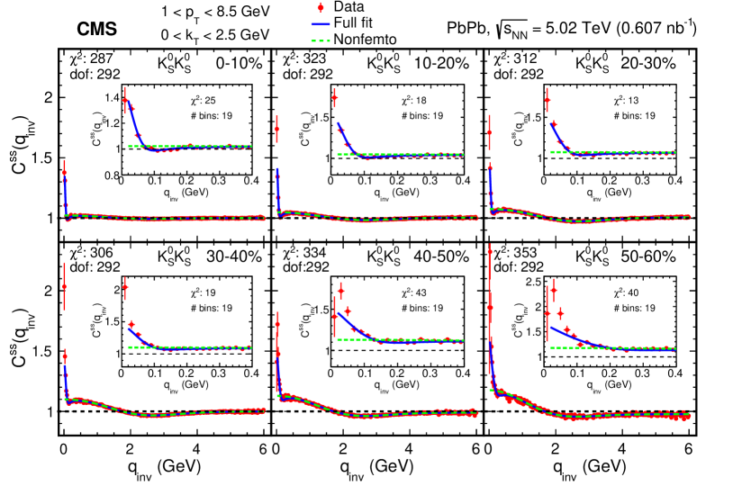
Figure 2: The correlation distributions and fits for $\PKzS\PKzS$ pairs in different centrality ranges, starting from 0–10% centrality to 50–60% centrality, with $0<\kt<2.5\GeV$. In each plot, the red circles are the data, the blue solid line is the fit using Eq. (8), and the green dotted line is the non-femtoscopic background from Eq. (7). The $\chi^{2}$ and $\mathrm{dof}$ values are for the full $q_{\text{inv}}$ range. The insert plots show the data and the fit for the $q_{\text{inv}}<0.4\GeV$ region, with the $\chi^{2}$ and number of bins evaluated in that region.

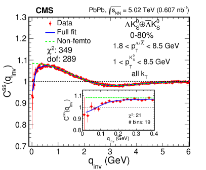
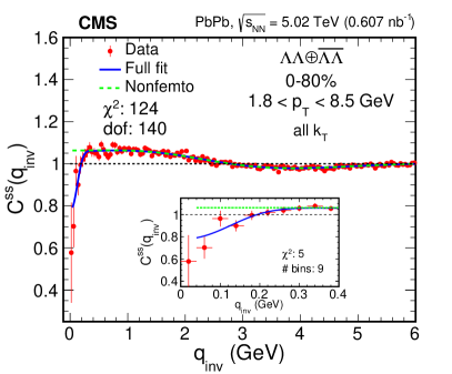
Figure 3: The correlation distributions and fits for $\PGL\PKzS$ (left) and $\PGL\PGL$ (right) pairs with 0–80% centrality and no restriction on . In each plot, the red circles are the data, the blue solid line is the fit using Eq. (8), and the green dotted line is the non-femtoscopic background from Eq. (7). The $\chi^{2}$ and $\mathrm{dof}$ values are for the full $q_{\text{inv}}$ range. The insert plots show the data and the fit for the $q_{\text{inv}}<0.4\GeV$ region, with the $\chi^{2}$ and number of bins evaluated in that region.

0.5 Systematic uncertainties

The systematic uncertainties for the fit parameters are based on the changes found in the parameter values after individually varying each of the analysis criteria, as discussed below. In cases with more than one variation for a single source, the maximum deviation from the nominal value is used. The total systematic uncertainty is obtained by adding the uncertainties from each source in quadrature. The BDT discriminant is varied so as to adjust the signal-to-background ratio, with the signal yield changing by $\pm$15% in the process. The nominal method to account for $\textrm{V}^{0}$ candidates sharing daughter tracks is to remove one of the $\textrm{V}^{0}$ candidates at random, which is then not used by any pair. Two alternative approaches are used, one in which both $\textrm{V}^{0}$ candidates are removed and another in which, for events with multiple $\textrm{V}^{0}$ candidate pair combinations, only the pairs in which the two particles share a daughter are removed. The systematic uncertainties related to $\textrm{V}^{0}$ signal and background modeling are investigated by varying the background shape from a fourth- to a third-order polynomial and the signal shape from a sum of three Gaussian functions to a sum of two or four Gaussian functions. An alternative non-femtoscopic background function $\Omega(q_{\text{inv}})=N(1+B\re^{-|q_{\text{inv}}/\sigma|^{2}})(1+\epsilon q_{\text{inv}})$ is used to assess the uncertainty associated with the choice of the non-femtoscopic background function. The selection requirements used to construct the mixed event sample are varied to require centrality matching of 3 and 7% instead of the nominal 5% and the primary vertex position matching with 1 and 3cm instead of the nominal 2cm. The effect of the centrality resolution has been checked and found to be negligible. The peak region requirement is changed from ${<}2.0\sigma$ to ${<}1.5\sigma$ and ${<}2.5\sigma$ and the sideband region selection from ${>}4.0\sigma$ to ${>}3.5\sigma$ and ${>}4.5\sigma$. The upper limit of the $q_{\text{inv}}$ fit ranges is changed by $\pm$1and the lower limit is changed to include the first bin. At low , the tracking efficiency is strongly dependent on . Therefore, the simulated sample is used to explore possible effects of the tracking efficiency. Based on these studies, it is found that the $\textrm{V}^{0}$ reconstruction efficiency for the detection of two $\textrm{V}^{0}$ particles is well described by taking the product of the efficiency for each $\textrm{V}^{0}$. It is also found that the fit results are only weakly affected by the $\textrm{V}^{0}$ reconstruction efficiency. This is understood as a consequence of the signal and reference samples being similarly affected by the $\textrm{V}^{0}$ efficiency. Differences in the Monte Carlo and experimental spectra could influence the cancellation of efficiency-dependent effects in the signal and background correlations. Therefore, a systematic uncertainty for the efficiency is assessed by comparing the results for the default simulated sample to one in which the $\textrm{V}^{0}$ distribution is reweighted to match the data. For the $\PKzS\PKzS$ correlations, an additional systematic uncertainty is found from varying the mass and coupling parameters for the $\PfDzP{980}$ and resonances by using rows A, B, and D of Table 1 of Ref. [40]. The systematic uncertainties are summarized in Table 0.5.

Summary of absolute systematic uncertainties in $\PKzS\PKzS$, $\PGL\PKzS$ and $\PGL\PGL$ correlation measurements. The values for $R_{\text{inv}}$, $d_{0}$, $\Re f_{0}$, and $\Im f_{0}$ are infm. Uncertainty source $\PKzS\PKzS$ $\PGL\PKzS$ $\PGL\PGL$ $R_{\text{inv}}$ $R_{\text{inv}}$ $d_{0}$ $\Re f_{0}$ $\Im f_{0}$ $R_{\text{inv}}$ $d_{0}$ $\Re f_{0}$ BDT cut 0.04–0.18 0.01–0.04 0.19 0.75 0.10 0.07 0.03 0.06 0.43 0.05 0.31 Duplicate $\textrm{V}^{0}$ removal 0.06–0.40 0.01–0.08 0.35 0.92 0.10 0.19 0.11 0.01 1.14 0.05 0.14 Mass fit function 0.00–0.01 0.00–0.01 0.09 0.05 0.01 0.03 0.03 0.02 0.04 0.01 0.02 Non-femtoscopic func. 0.02–0.16 0.01–0.12 0.02 0.17 0.05 0.07 0.03 0.02 1.02 0.14 0.93 Reference sample 0.03–0.08 0.01–0.05 0.22 0.48 0.12 0.12 0.03 0.10 1.12 0.20 0.76 Peak region 0.00–0.07 0.01–0.02 0.43 0.10 0.05 0.17 0.08 0.22 1.21 0.08 0.35 Sideband region 0.00–0.03 0.00–0.01 0.02 0.02 0.01 0.01 0.00 0.01 0.03 0.01 0.04 Fitting range 0.01–0.11 0.01–0.04 0.20 0.18 0.03 0.08 0.04 0.04 1.79 0.20 0.60 Efficiency 0.03–0.03 0.01–0.01 0.08 0.29 0.06 0.09 0.03 0.02 0.05 0.03 0.04 $\PfDzP{980}$/param. 0.07–0.39 0.03–0.05 Total uncertainty 0.29–0.47 0.08–0.16 0.69 1.34 0.21 0.32 0.16 0.25 2.91 0.34 1.43

0.6 Results

The size of the particle emitting source $R_{\text{inv}}$ and the parameter extracted from the $\PKzS\PKzS$ correlations for $0<\kt<2.5\GeV$ are shown as a function of centrality in Fig. 4. It is observed that the $R_{\text{inv}}$ value decreases from central to peripheral events, as expected from a simple geometric picture of the collisions. Over the full centrality range of 0–80%, $R_{\text{inv}}=3.30\pm 0.10\stat\pm 0.37\syst$fm. The transverse mass can be calculated as $\mT=\sqrt{\smash[b]{(m_{\text{inv}}/2)^{2}+\kt^{2}}}$, where $m_{\text{inv}}$ is the invariant mass of the two-particle system [15]. The average $\left<\mT\right>$ is evaluated from the transverse mass distribution using two-particle pairs with $q_{\text{inv}}<0.4\GeV$, accounting for background using the binomial analysis as done for the $q_{\text{inv}}$ distributions. Our results for $R_{\text{inv}}$ agree with the ALICE $\PKzS\PKzS$ results from PbPb collisions at $\sqrtsNN=2.76\TeV$ at a similar value [47]. The parameter is seen to decrease from about 0.45 to 0.25 as the collisions become more peripheral. This decrease could arise from a relative increase in the contribution from resonance decays or a source function that becomes increasingly non-Gaussian as the collisions become more peripheral. The assumption of a Gaussian source function in the LL model may also be responsible for the relatively poor fits at low $q_{\text{inv}}$ for the most peripheral collisions, as seen in Fig. 2.

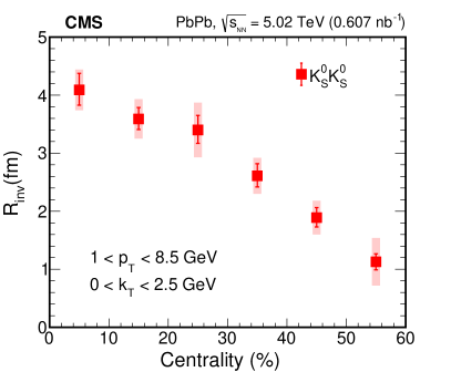
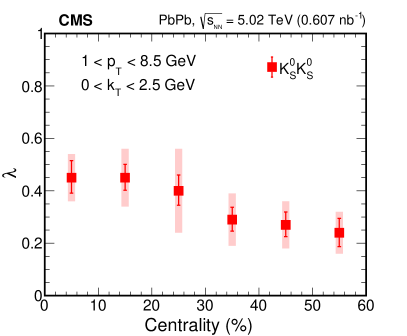
Figure 4: The $R_{\text{inv}}$ (left) and parameter (right) as a function of centrality. For each data point, the line and shaded area indicate the statistical and systematic uncertainty, respectively.

Table 0.6 includes the extracted $R_{\text{inv}}$ and parameters as well as $\left<\mT\right>$ for $\PKzS\PKzS$, $\PGL\PKzS$, and $\PGL\PGL$ combinations in the 0–80% centrality range. A significant decrease is seen in $R_{\text{inv}}$ as the $\left<\mT\right>$ increases. Qualitatively similar results have been found, both for a given pair type in bins of and when comparing multiple pair types [1]. Because of the different minimum requirements for and particles, the variation in $\left<\mT\right>$ includes both $\left<\pt\right>$ and particle mass differences. The anticorrelation of $R_{\text{inv}}$ and $\left<\mT\right>$ has been interpreted as indicating the presence of an expanding source [1].

Table 0.6 also includes the strong interaction scattering parameters $d_{0}$, $\Re f_{0}$, and $\Im f_{0}$ obtained from the $\PGL\PKzS$ and $\PGL\PGL$ correlations. Figure 5 shows $d_{0}$ and $\Im f_{0}$ versus $\Re f_{0}$ in the left and right panels, respectively, with the current results shown as red stars and squares for $\PGL\PKzS$ and $\PGL\PGL$, respectively. The displayed uncertainties are one-dimensional and are not based on a two-dimensional contour.

Extracted values of the $R_{\text{inv}}$, $\Re f_{0}$, $\Im f_{0}$, $d_{0}$, , and $\left<\mT\right>$ parameters from the $\PKzS\PKzS$, $\PGL\PKzS$, and $\PGL\PGL$ combinations in the 0–80% centrality range. The first and second uncertainties are statistical and systematic, respectively. Parameter $\PKzS\PKzS$ $\PGL\PKzS$ $\PGL\PGL$ $R_{\text{inv}}$ (fm) $3.30\pm 0.10\pm 0.37$ $2.1^{+1.4}_{-0.5}\pm 0.7$ $1.3^{+0.4}_{-0.2}\pm 0.3$ $\Re f_{0}$ (fm) $-0.76^{+0.29}_{-0.19}\pm 0.21$ $0.74^{+0.59}_{-0.16}\pm 0.34$ $\Im f_{0}$ (fm) $-0.07^{+0.48}_{-0.11}\pm 0.32$ $d_{0}$ (fm) $2.3^{+0.7}_{-0.5}\pm 1.3$ $4.2^{+5.7}_{-2.1}\pm 2.9$ $0.38\pm 0.02\pm 0.08$ $0.34^{+0.41}_{-0.12}\pm 0.16$ $1.5^{+1.2}_{-1.1}\pm 1.4$ $\left<\mT\right>$ () 1.53 2.09 2.60

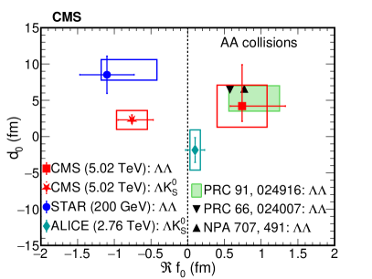
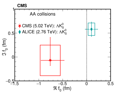
Figure 5: The measured values of $d_{0}$ versus $\Re f_{0}$ (left) and $\Im f_{0}$ versus $\Re f_{0}$ (right) from this analysis along with other measurements and predictions as described in the text. For each data point, the lines and the boxes indicate the (one-dimensional) statistical and systematic uncertainties, respectively.

The negative value of $\Re f_{0}$ observed for the $\PGL\PKzS$ correlations, combined with its relatively small magnitude, suggests a repulsive $\PGL\PKzS$ interaction. The uncertainty associated with the $\Im f_{0}$ value for the $\PGL\PKzS$ correlations prevents any claim concerning possible inelastic processes. The value of $\Re f_{0}$ found for $\PGL\PKzS$ correlations differs from that reported by the ALICE Collaboration (teal diamonds) [15], which is also for PbPb collisions but at $\sqrtsNN=2.76\TeV$. The uncertainties are too large to determine if $d_{0}$ and $\Im f_{0}$ also differ between the two results.

The positive $\Re f_{0}$ value obtained for the $\PGL\PGL$ correlations suggests an attractive interaction that is not strong enough to produce a bound state such as the H-dibaryon [9, 48]. This result disagrees with the finding from the STAR Collaboration in gold-gold (AuAu) collisions at $\sqrtsNN=200\GeV$ (blue circle). The negative $\Re f_{0}$ value of ${-}1.10\pm 0.37\stat^{+0.68}_{-0.08}\syst$fm found by STAR, combined with its magnitude, imply a repulsive interaction. It is noted, however, that a theoretical study of the STAR data which considers collective flow and feed-down effects (shown as a shaded region at $d_{0}\approx 5$fm, $\Re f_{0}\approx 0.9$fm) suggests that these data are consistent with the $\PGL\PGL$ interaction being attractive [9]. An exclusion plot by the ALICE Collaboration for the $\PGL\PGL$ scattering parameters obtained using the $\PGL\PGL$ correlations from $\Pp\Pp$ collisions at $\sqrt{s}=7$ and 13, as well as $\Pp\text{Pb}$ collisions at $\sqrtsNN=5.02\TeV$, also suggests an attractive interaction [10]. In addition, our results are consistent with two theoretical calculations (black triangles) that reproduce the $\PGL\PGL$ binding energy of ${}^{\;\;\;\;6}_{\PGL\PGL}{\mathrm{He}}$, as extracted from the NAGARA event [49, 50].

0.7 Summary

The $\PKzS\PKzS$, $\PGL\PKzS$, and $\PGL\PGL$ femtoscopic correlations are studied using lead-lead (PbPb) collision data at a center-of-mass energy per nucleon pair of $\sqrtsNN=5.02\TeV$, collected by the CMS Collaboration. This is the first report on $\PGL\PGL$ correlations in PbPb collisions at the CERN LHC. The source size $R_{\text{inv}}$ and the incoherence parameter were extracted for $\PKzS\PKzS$ correlations in six centrality bins covering the 0–60% range. The value of $R_{\text{inv}}$ decreases from 4 to 1fm going from central to peripheral collisions and agrees with results from the ALICE Collaboration at a similar transverse mass. Along with the $R_{\text{inv}}$ and parameters, the strong interaction scattering parameters, , the complex scattering length and effective range, were extracted from $\PGL\PKzS$ and $\PGL\PGL$ correlations in the 0–80% centrality range. These scattering parameters indicate that the $\PGL\PKzS$ interaction is repulsive and that the $\PGL\PGL$ interaction is attractive. The scattering parameters obtained from $\PGL\PKzS$ correlations differ from those reported by the ALICE Collaboration. The positive real scattering length obtained from the $\PGL\PGL$ correlation disfavors the existence of a bound H-dibaryon state. The $\PGL\PGL$ scattering parameters help to constrain baryon-baryon and, more specifically, hyperon-hyperon interaction models. These measurements provide an additional input to understand the nature of the strong interaction between pairs of strange hadrons.

References

- [1] M. A. Lisa, S. Pratt, R. Soltz, and U. Wiedemann, “Femtoscopy in relativistic heavy ion collisions: Two decades of progress”, Ann. Rev. Nucl. Part. Sci. 55 (2005) 357, 10.1146/annurev.nucl.55.090704.151533, arXiv:nucl-ex/0505014.
- [2] V. G. J. Stoks, R. A. M. Klomp, M. C. M. Rentmeester, and J. J. de Swart, “Partial-wave analysis of all nucleon-nucleon scattering data below 350 MeV”, Phys. Rev. C 48 (1993) 792, 10.1103/PhysRevC.48.792.
- [3] J. J. de Swart and C. Dullemond, “Effective range theory and the low energy hyperon-nucleon interactions”, Anna. Phys. 19 (1962) 458, 10.1016/0003-4916(62)90185-9.
- [4] R. Engelmann, H. Filthuth, V. Hepp, and E. Kluge, “Inelastic \PGSm\Pp-interactions at low momenta”, Phys. Lett. 21 (1966) 587, 10.1016/0031-9163(66)91310-2.
- [5] F. Eisele et al., “Elastic \PGSpm\Pp scattering at low energies”, Phys. Lett. B 37 (1971) 204, 10.1016/0370-2693(71)90053-0.
- [6] B. Sechi-Zorn, B. Kehoe, J. Twitty, and R. A. Burnstein, “Low-energy \PGL-proton elastic scattering”, Phys. Rev. 175 (1968) 1735, 10.1103/PhysRev.175.1735.
- [7] CMS Collaboration, “Bose–Einstein correlations in pp, pPb, and PbPb collisions at ”, Phys. Rev. C 97 (2018) 064912, 10.1103/PhysRevC.97.064912, arXiv:1712.07198.
- [8] J. Schaffner-Bielich, M. Hanauske, H. Stöcker, and W. Greiner, “Phase transition to hyperon matter in neutron stars”, Phys. Rev. Lett. 89 (2002) 171101, 10.1103/PhysRevLett.89.171101, arXiv:astro-ph/0005490.
- [9] K. Morita, T. Furumoto, and A. Ohnishi, “ interaction from relativistic heavy-ion collisions”, Phys. Rev. C 91 (2015) 024916, 10.1103/PhysRevC.91.024916, arXiv:1408.6682.
- [10] ALICE Collaboration, “Study of the \PGL-\PGL interaction with femtoscopy correlations in pp and pPb collisions at the LHC”, Phys. Lett. B 797 (2019) 134822, 10.1016/j.physletb.2019.134822, arXiv:1905.07209.
- [11] R. L. Jaffe, “Perhaps a stable dihyperon”, Phys. Rev. Lett. 38 (1977) 195, 10.1103/PhysRevLett.38.195.
- [12] H. Takahashi et al., “Observation of a double hypernucleus”, Phys. Rev. Lett. 87 (2001) 212502, 10.1103/PhysRevLett.87.212502.
- [13] K. Nakazawa and H. Takahashi, “Experimental study of double-\PGL hypernuclei with nuclear emulsion”, Prog. Theor. Phys. Supplement 185 (2010) 335, 10.1143/PTPS.185.335.
- [14] Belle Collaboration, “Search for an -dibaryon with a mass near in \PgUa and \PgUb decays”, Phys. Rev. Lett. 110 (2013) 222002, 10.1103/PhysRevLett.110.222002, arXiv:1302.4028.
- [15] ALICE Collaboration, “ femtoscopy in Pb-Pb collisions at ”, Phys. Rev. C 103 (2021) 055201, 10.1103/PhysRevC.103.055201, arXiv:2005.11124.
- [16] C. Loizides, J. Kamin, and D. d’Enterria, “Improved Monte Carlo Glauber predictions at present and future nuclear colliders”, Phys. Rev. C 97 (2018) 054910, 10.1103/PhysRevC.97.054910, arXiv:1710.07098.
- [17] R. Lednický and V. L. Lyuboshitz, “Final state interaction effect on pairing correlations between particles with small relative momenta”, Sov. J. Nucl. Phys. 35 (1982) 770.
- [18] HEPData record for this analysis, 2022. 10.17182/hepdata.133573.
- [19] Tracker Group of the CMS Collaboration, “The CMS phase-1 pixel detector upgrade”, JINST 16 (2021) P02027, 10.1088/1748-0221/16/02/P02027, arXiv:2012.14304.
- [20] CMS Collaboration, “Track impact parameter resolution for the full pseudorapidity coverage in the 2017 dataset with the CMS phase-1 pixel detector”, CMS Detector Performance Note CMS-DP-2020-049, 2020.
- [21] CMS Collaboration, “Performance of the CMS level-1 trigger in proton-proton collisions at ”, JINST 15 (2020) P10017, 10.1088/1748-0221/15/10/P10017, arXiv:2006.10165.
- [22] CMS Collaboration, “The CMS trigger system”, JINST 12 (2017) 01020, 10.1088/1748-0221/12/01/P01020, arXiv:1609.02366.
- [23] CMS Collaboration, “The CMS experiment at the CERN LHC”, JINST 3 (2008) S08004, 10.1088/1748-0221/3/08/S08004.
- [24] CMS Collaboration, “Precision luminosity measurement in proton-proton collisions at in 2015 and 2016 at CMS”, Eur. Phys. J. C 81 (2021) 800, 10.1140/epjc/s10052-021-09538-2, arXiv:2104.01927.
- [25] CMS Collaboration, “CMS luminosity measurement using nucleus-nucleus collisions at in 2018”, CMS Physics Analysis Summary CMS-PAS-LUM-18-001, 2022.
- [26] CMS Collaboration, “Charged-particle nuclear modification factors in PbPb and pPb collisions at ”, JHEP 04 (2017) 039, 10.1007/JHEP04(2017)039, arXiv:1611.01664.
- [27] CMS Collaboration, “Description and performance of track and primary-vertex reconstruction with the CMS tracker”, JINST 9 (2014) P10009, 10.1088/1748-0221/9/10/p10009, arXiv:1405.6569.
- [28] CMS Collaboration, “Transverse-momentum and pseudorapidity distributions of charged hadrons in pp collisions at and 2.36 TeV”, JHEP 02 (2010) 041, 10.1007/JHEP02(2010)041, arXiv:1002.0621.
- [29] CMS Collaboration, “Observation and studies of jet quenching in PbPb collisions at nucleon-nucleon ”, Phys. Rev. C 84 (2011) 024906, 10.1103/PhysRevC.84.024906, arXiv:1102.1957.
- [30] C. Gale, S. Jeon, and B. Schenke, “Hydrodynamic modeling of heavy ion collisions”, Int. J. Mod. Phys. A 28 (2013) 1340011, 10.1142/S0217751X13400113, arXiv:1301.5893.
- [31] GEANT4 Collaboration, “\GEANTfour—a simulation toolkit”, Nucl. Instrum. Meth. A 506 (2003) 250, 10.1016/S0168-9002(03)01368-8.
- [32] CMS Collaboration, “Strange hadron collectivity in pPb and PbPb collisions”, 2022. arXiv:2205.00080.
- [33] CMS Collaboration, “Strange particle production in pp collisions at and 7 TeV”, JHEP 05 (2011) 064, 10.1007/JHEP05(2011)064, arXiv:1102.4282.
- [34] CMS Collaboration, “Long-range two-particle correlations of strange hadrons with charged particles in pPb and PbPb collisions at LHC energies”, Phys. Lett. B 742 (2015) 200, 10.1016/j.physletb.2015.01.034, arXiv:1409.3392.
- [35] Particle Data Group Collaboration, “Review of particle physics”, Prog. Theor. Exp. Phys. 2022 (2022) 083C01, 10.1093/ptep/ptac097.
- [36] H. Voss, A. Höcker, J. Stelzer, and F. Tegenfeldt, “TMVA, the toolkit for multivariate data analysis with ROOT”, in XIth International Workshop on Advanced Computing and Analysis Techniques in Physics Research (ACAT), p. 40. 2007. arXiv:physics/0703039. 10.22323/1.050.0040.
- [37] G. I. Kopylov, “Like particle correlations as a tool to study the multiple production mechanism”, Phys. Lett. B 50 (1974) 472, 10.1016/0370-2693(74)90263-9.
- [38] A. Kisiel, “Non-identical particle correlation analysis in the presence of non-femtoscopic correlations”, Acta Phys. Polon. B 48 (2017) 717, 10.5506/APhysPolB.48.717.
- [39] ALICE Collaboration, “pp, p-\PGL, and \PGL-\PGL correlations studied via femtoscopy in pp reactions at ”, Phys. Rev. C 99 (2019) 024001, 10.1103/PhysRevC.99.024001, arXiv:1805.12455.
- [40] STAR Collaboration, “Neutral kaon interferometry in Au+Au collisions at ”, Phys. Rev. C 74 (2006) 054902, 10.1103/PhysRevC.74.054902, arXiv:nucl-ex/0608012.
- [41] A. D. Martin and E. N. Ozmutlu, “Analyses of production and scalar mesons”, Nucl. Phys. B 158 (1979) 520, 10.1016/0550-3213(79)90180-9.
- [42] A. Antonelli, “Radiative \PGf decays”, eConfC 020620 (2002) THAT06, 10.48550/ARXIV.HEP-EX/0209069, arXiv:hep-ex/0209069.
- [43] N. N. Achasov and V. V. Gubin, “Analysis of the nature of the and decays”, Phys. Rev. D 63 (2001) 094007, 10.1103/PhysRevD.63.094007, arXiv:hep-ph/0101024.
- [44] N. N. Achasov and A. V. Kiselev, “New analysis of the KLOE data on the decay”, Phys. Rev. D 68 (2003) 014006, 10.1103/PhysRevD.68.014006, arXiv:hep-ph/0212153.
- [45] F. James and M. Roos, “Minuit: A system for function minimization and analysis of the parameter errors and correlations”, Comput. Phys. Commun. 10 (1975) 343, 10.1016/0010-4655(75)90039-9.
- [46] PHENIX Collaboration, “Lévy-stable two-pion Bose–Einstein correlations in Au+Au collisions”, Phys. Rev. C 97 (2018) 064911, 10.1103/PhysRevC.97.064911, arXiv:1709.05649.
- [47] ALICE Collaboration, “One-dimensional pion, kaon, and proton femtoscopy in Pb-Pb collisions at ”, Phys. Rev. C 92 (2015) 054908, 10.1103/PhysRevC.92.054908, arXiv:1506.07884.
- [48] STAR Collaboration, “ correlation function in Au+Au collisions at ”, Phys. Rev. Lett. 114 (2015) 022301, 10.1103/PhysRevLett.114.022301, arXiv:1408.4360.
- [49] E. Hiyama et al., “Four-body cluster structure of double-\PGL hypernuclei”, Phys. Rev. C 66 (2002) 024007, 10.1103/physrevc.66.024007, arXiv:nucl-th/0204059.
- [50] I. N. Filikhin and A. Gal, “Faddeev–Yakubovsky calculations for light hypernuclei”, Nucl. Phys. A 707 (2002) 491, 10.1016/s0375-9474(02)01008-4, arXiv:nucl-th/0203036.