Entanglement negativity in de Sitter biverse from Stringy Axionic Bell pair: An analysis using Bunch-Davies vacuum

Sayantan Choudhury1 Corresponding author, E-mail : sayantan_ccsp@sgtuniversity.org, sayanphysicsisi@gmail.com, §§§ NOTE: This project is the part of the non-profit virtual international research consortium “Quantum Aspects of Space-Time & Matter” (QASTM) . ,.

1Centre For Cosmology and Science Popularization (CCSP), SGT University, Gurugram, Delhi-NCR, Haryana- 122505, India.


Abstract

In this work, we study the signatures of quantum entanglement by computing entanglement negativity between two causally unrelated regions in 3+1313+1 dimensional global de Sitter space. We investigate a bipartite quantum field theoretic setup for this purpose, driven by an axionic Bell pair resulting from Type IIB string compactification on a Calabi-Yau three fold. We take into account a spherical surface that divides the spatial slice of the global de Sitter space into exterior and interior causally unrelated sub regions. For the computational purpose we use the simplest possible initial choice of quantum vacuum, which is Bunch-Davies state. The quantitative quantum information theoretic measure for entanglement negativity turns out be consistent with the results obtained for entanglement entropy, even we have to say it is better than that from quantum information theoretic point of view. We design the problem in a hyperbolic open chart where one of the causally unrelated observers remains constrained and the scale dependence enters to the corresponding quantum information theoretic entanglement measure for axionic Bell pair. We find from our analysis that in the large scales initially maximally entangled Bunch-Davies state turns out to be strongly entangled or weakly entangled depending on the axionic decay constant and the supersymmetry breaking scale. We also find that at the small scales the initial entanglement can be perfectly recovered. We also discuss the possibility of having a biverse picture, which is a mini version of the multiverse in the present theoretical set up. Last but not the least, we provide the necessary criteria for generating non vanishing quantum entanglement measures within the framework of quantum field theory of global de Sitter space as well as well as in primordial cosmology due to the axion derived from string theory.


Keywords:  De-Sitter vacua, Quantum Entanglement, Cosmology of Theories beyond
the SM, Quantum Information Theory aspects of Gravity, String Cosmology.

1 Introduction

In the present day research, different quantum information theoretic measures of quantum entanglement is a remarkable probe in theoretical physics which helps us to distinguish the various type of long range correlated quantum mechanical states. In this connection, study of the explicit role of the long range quantum correlations in the framework of quantum field theory is extremely significant, which is a fascinating topic of research itself. See refs [1, 2, 3, 4, 5, 6, 7, 8, 9, 10, 11, 12, 13, 14, 15, 16, 17, 18, 19, 20, 21, 22, 23, 24, 25, 26, 27, 28, 29, 30, 31] for more details. The key ingredient of this study is the initial quantum mechanical vacuum states, which are Chernikov-Tagirov, Bunch-Davies, Hartle-Hawking, α𝛼\alpha and Motta-Allen vacua [32, 33, 34, 35, 36, 16, 15, 37, 14, 19]. Quantum entanglement is treated as one of the remarkable outcomes of the foundational theoretical aspects of quantum mechanics. The prime reason of this thought is, a local measurement in quantum mechanics may instantaneously put a significant impact of the outcome of the measurement beyond the physical light cone. This is theoretically interpreted as Einstein-Podolsky-Rosen (EPR) paradox where the concept of causality violation is explicitly demonstrated [38, 39, 40, 41, 31].

Amongst various types of information theoretic measures entanglement entropy is considered to be a very useful quantitative as well as qualitative probe of quantum entanglement and this concept is commonly used in the framework of condensed matter physics, quantum information theory and high energy physics. But in this connection it is important to note that the technical computation of entanglement entropy is very difficult to perform in the context of quantum field theory. Ryu and Takayanagi in refs. [42, 43] first did the theoretically consistent computation of entanglement entropy for a strongly coupled quantum field theory having a gravitational dual counterpart using the underlying physical principles of AdS/CFT (or holographic gravitational dual prescription) [44].

In order to properly understand the direct implications of the previously proposed AdS/CFT (or holographic gravitational dual prescription) in the technical computation of entanglement entropy in presence of standard Bunch-Davies quantum vacuum state within the framework of quantum field theory of de Sitter space, Maldacena and Pimentel prescribed an extremely useful computational strategy in ref. [1] using free massive scalar quantum field. After this work the proposed methodology was generalised for the same problem in presence of non standard α𝛼\alpha vacua in refs [45, 46, 47, 13, 19]. Further in refs. [14, 15, 16], these underlying physical concepts of the computation of entanglement entropy was applied within the framework of axion quantum field theory, described in terms a specific type of effective interaction potential originated from Type II string theory compactification [48, 49, 50] in presence of both standard Bunch-Davies and non standard α𝛼\alpha quantum vacua. The underlying concept of quantum entanglement could applicable to the framework of cosmology, specifically beyond the Hubble horizon scale. Most importantly, in this prescription if a particle pair is created in a casually connected Hubble horizon scale then it is naturally expected to be dissociated as an outcome of the de Sitter cosmological expansion. In this particular case, the findings from this prescription pointing towards the fact that two causally unrelated patches in the de Sitter cosmological space-time has to be entangled quantum mechanically. As a result, the corresponding observable quantum vacuum fluctuations associated with our own universe is entangled with the other part of the open patch of global de Sitter space, which is commonly identified to be the multiverse in the present context of discussion. To demonstrate this underlying physical picture the reduced density matrix formalism play a very significant role, using which it was explicitly obtained that the quantum mechanical entanglement directly put impact on the cosmological power spectrum on the large scales and it is quantitatively similar to or larger than the curvature radius scale connected to the current issue [18].

It is hugely expected that the present and the upcoming observational probes may detect the imprints and explicit effects of quantum mechanical entanglement in cosmological paradigm, which we strongly believe will going to be extremely useful to understand a lot of unknown mysterious fascinating facts of our own universe. In the past, there are lot of efforts have been made to study the impacts of quantum mechanical entanglement in the theoretical framework of cosmology. See refs. [18, 16, 51, 21, 52, 23, 53, 54, 55, 56, 57, 58] for more details on these aspects.

The motivation of the background physical thought of the present paper are appended below point-wise:

  1. 1.

    It was first discovered in a number of refs.[59, 60, 61] to support the claim that the physical frame of the bubble nucleation process is observer dependent and is actually dictated by the rest frame of the observer. The bubble nucleation process being dependent on the observer is hence only expected. The detailed study of such type of observer dependence in the framework of quantum mechanical entanglement is one of the prime motivations of the present work. If one can able to address this issue in detail, then various unexplored features of quantum cosmology can be explored with proper physical understanding.

  2. 2.

    Second, the explicit function of the Bunch Davies vacuum can be investigated in the context of quantum entanglement originating from an axion field embedded in an open patch of the global de Sitter space. This will be crucial because it allows one to directly examine whether it is possible to find the signs of quantum entanglement in the current multiverse [18, 62, 63, 64, 65, 66, 67] motivated theoretical set up.using current or future observational instruments.

  3. 3.

    Thirdly, it was noted in the refs. [68, 69, 70, 14, 15, 16] that the string theory-originated axion can be viewed as the ideal component to build the Bell pair, which is necessary to violate Bell’s inequality within the context of primordial cosmology. Within the widely accepted framework of primordial cosmology, it is virtually difficult to break Bell’s inequality, and it is for this reason that string theory and the axion play the most important roles. It is significant to note that, in this context, it is nearly impossible to test the explicit role of quantum mechanical entanglement in observational probes without violating Bell’s inequality in the context of primordial cosmology, which is necessary to break the degeneracy in the shape cosmological two-point function, also known as the primordial power spectrum obtained from various effective potentials from fundamental physical principles. The current framework with the string theory-originated axion provides a perfect setup that is pointing towards a new physics coming from a non-standard cosmology because the generation of Bell’s inequality violating pairs, also known as the Bell pair, is practically impossible within the framework of the standard primordial cosmological paradigm. It is explicitly pointed in refs.[68, 69, 70] that the prime signature of the Bell’s inequality violation in non standard primordial cosmology is coming from the existence of one point function from axion, which is absent in the well known standard cosmological paradigm. This result has a great impact of producing quantum entanglement in the present scenario. Also our derived results can be extremely useful to directly verify along with the observational probes the applicability as well as the justifiability of the string theory originated axion to address the issue of quantum entanglement in the present set up. See refs. [71, 72, 73, 74, 75, 68, 69, 70, 14, 15, 16, 76, 77] for more details on the Bell’s inequality and its violation in various contexts including cosmology.

  4. 4.

    Finally, the motivation comes from the multiverse prescription appearing in the string theory landscape scenario, which states that our universe may not be the single entity of the space-time but the part of a bigger size multiverse [18, 62, 63, 64, 65, 66, 67]. This is obviously a fascinating fact which one needs to study in detail. However, in the past the underlying physical concept of the multiverse has been criticised in various contexts as a hypothetical philosophical concept which is the outcome of complete theoretical imagination and cannot be tested via cosmological observation. But the actual truth is fay beyond all of these criticism, which is the detectable signatures can be obtained from the multiverse set up in presence of quantum mechanical entanglement. It really helps us to produce at least two causally separated de sitter universe, commonly known as the de Sitter bubbles in the present context. But the numbers are not restricted in two and most importantly this is actually the starting point of multiverse which allows many more causally unrelated de Sitter bubbles.

Next, we explicitly write down the underlying assumptions of the present work, which are appended below point-wise:

  1. 1.

    To model the present multiverse motivated scenario [18, 62, 63, 64, 65, 66, 67] , we consider two causally separated patches on the global de Sitter space by assuming that initially they are in a maximally entangled pure quantum mechanical state. this particular set up we identify as the biverse picture which is the mini version of the original multiverse picture.

  2. 2.

    In this theoretical set up further we introduce two observers whose actual purpose is to determine the quantum entanglement of a de Sitter universe. We also assume that one of the observers is placed inside the a de Sitter bubble and want to determine how the signatures of quantum mechanical entanglement with the other de Sitter bubble can be visualized by the inside observer. Now the issue is that, the inside observer can’t able to see outside region of their own de Sitter bubble. For this reason instead of using the total density matrix, one needs to take the partial trace over the causally unrelated outside region, which finally give rise to the reduced density matrix of the system in the present context. But as an outcome some information will be lost during this process and to describe the quantum mechanical state of the observer instead of using a pure state one needs to explicitly use a mixed state. This scenario is completely different for an observer who is sitting on the other causally separated de Sitter bubble because in his frame of reference the quantum aspects is described by the pure quantum states. For this reason we need study the effects and outcomes of the quantum entanglement between pure and mixed states in the present context of discussion.

  3. 3.

    To perform the computation for a single global de Sitter space picture as well in the case of the entangled two de Sitter space, which is the biverse picture we need to properly understand the factorization of the Hilbert space in terms of the individual constituents which span the subspaces by forming complete orthonormal sets. The geometrical structure of the global de Sitter space demands that in the hyperbolic open chart one can symmetrically factorize in the left region and in a right region, which we have tagged as region L and R during performing the technical computation in this paper. Since we have symmetrically factorize the total Hilbert space in the region L and R, it is viable to formulate the reduced description either in terms of the degrees of freedom appearing in the region L or region R. In our computation we take the partial trace over the degrees of freedom appearing in the region R, which forms a reduced density matrix in the region L.

  4. 4.

    If the Hilbert space factorization performed correctly then one can further blindly trust the mode decomposition in the region L and R using which we have constructed the Bunch Davies quantum vacuum states in terms of harmonic oscillator modes which forms a complete orthonormal basis states. Estimation of the quantum entanglement in terms of various quantum information theoretic measures are also based on this mode decomposition and hence one can rely on the tracing out the unwanted information from the bipartite quantum field theoretic set up under consideration to construct the reduced density matrix.

  5. 5.

    To study the outcome of quantum mechanical entanglement we have blindly trusted the above mentioned factorization for the second de Sitter space which is spanned by the well known Bunch Davies vacuum state. For the other, which is the first de Sitter bubble we have assumed that the detailed factorization structure is not explicitly needed for the computation we are interested to perform in this paper. This is because of the fact that we need to take the partial trace operation over the first de Sitter vacuum which will remove all unwanted degrees of freedom from the quantum information theoretic measures of entanglement we want to compute to confirm the existence of quantum entanglement in the biverse picture. Here one can do the computation in other way as well where one needs to take the partial trace operation with respect to the all degrees of freedom appearing in second de Sitter vacuum and properly factorize the first de Sitter vacuum in terms of L and R modes. Due to having the symmetrical structure of the set up that we are considering it is expected that for both the cases we will have the same physical outcome at the end of the computation. We just have taken the first possibility as a choice.

  6. 6.

    During the biverse construction we have first constructed the maximally entangled state which is one of the key ingredients to violate the Bell’s CHSH inequality within the present framework. This is a very challenging to construct within the framework of de Sitter space time as well as in primordial cosmology set up. We have constructed the maximally entangled state which suffice the purpose. But this could not be possible just having usual interaction in the scalar field theory embedded in the global patch of the de Sitter space. The Bell’s CHSH inequality violating pair is created in the region L and R with the help of specific type of interaction in the string theory originated axion driven scalar field theory. The structure of the interaction is controlled by the time dependent axion decay constant and the supersymmetry breaking scale. We have assumed that Bell pair is created and originated from the string theory originated axionic scalar field theory. It might be possible to create such pair from some other theoretical sector as well which we have not considered in this paper for the time being.

  7. 7.

    In the present context the global coordinates can be treated as the closed slicing from the point of view of FLRW cosmology. One usually do primordial cosmology, particularly inflation [78, 79, 80, 81, 82, 83, 84, 85, 86, 87, 88, 89, 90, 91, 92, 93, 94, 95, 96, 97, 98, 99, 100, 101, 102, 103, 104, 105, 106, 107, 108, 109, 110, 111, 112, 113, 114, 115, 116] in the planar coordinate slicing of the de Sitter space. By performing coordinate coordinate transformation one can transform the global to static and then static to the flat slicing in the planer patch of de Sitter space. For this reason whatever results we have obtained in this paper for the global patch of the de Sitter space can be directly translated in the planer patch of the de Sitter space, which further implies that our derived results hold good for primordial cosmological set up constructed out of the effective interaction studied for the string theory originated axion scalar field theory. This is obviously an interesting aspect from our computation which shows the applicability of our derived results in the vast theoretical framework.

  8. 8.

    The von Neumann and Renyi entropies [117, 15, 14] are the good quantum information theoretic measures of quantum entanglement in the context of bipartite quantum field theory designed in terms of pure state. But with the help of mixed state if we want to understand the features of an arbitrary bipartite quantum field theoretic system then instead of using entropic measures, negativity or its logarithmic version would be perfect information theoretic measure of quantum entanglement. Using this specific measure we compute the imprints of the quantum entanglement from the point of view of two causally separated observers in the open chart of global de Sitter space.
Refer to caption
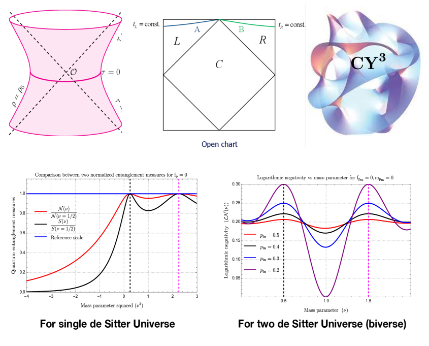
Figure 1.1: Representative diagram of the overall quantum entanglement computation and all possible outcomes for single de Sitter universe and two de Sitter universe (biverse) obtained from our our analysis.

In this work, we compute the negativitity measure of quantum entanglement from an axionic effective potential which is obtained from Type IIB string theory compactification on a Calabi-Yau three fold in presence of NS5 brane. Earlier this model have been studied in the framework of inflationary cosmology [118, 119, 120, 121]. Since this axions can be treated as Bell pair, we technically compute the expression for entanglement negativity from two causally unrelated patches of the open chart of the global de Sitter space. From the quantitative results obtained from our computation we perform further a consistency check as well as the comparison of the results obtained in previous refs.[14, 15, 16]. Furthermore, to understand various unknown fascinating facts regarding the multiverse scenario we extend our computation in presence of axionic Bell pair in presence of de Sitter space along with the maximally entangled quantum Bunch Davies vacuum state. We find from our analysis that in the large scales initially maximally entangled Bunch-Davies state turns out to be strongly entangled or weakly entangled depending on the axionic decay constant and the supersymmetry breaking scale. We also find the at the small scales the initial entanglement can be perfectly recovered. Last but not the least, we provide the necessary criteria for generating non vanishing quantum entanglement measure within the framework of primordial cosmology due to the string axion. In figure (1.1) representative diagram of the overall quantum entanglement computation and all possible outcomes for single de Sitter universe and two de Sitter universe (biverse) obtained from our our analysis.

The organization of this paper is as follows:

  • In Section 2 we briefly review the tools and techniques required to compute negativity and logarithmic negativity along with some easy demonstrations for the better understanding purpose.

  • In Section 3 we mention the computational strategy for negativity in the hyperbolic open chart of the global de Sitter space.

  • In Section 4 we compute negativity by following aforementioned strategy for a specific effective potential, Type IIB string compactification originated axion model.

  • In Section 5 we compute entanglement in terms of negativity from two causally unrelated de Sitter bubbles, which is determined from the point of view of two observers introduced during the calculation. In this section we discuss the possibility of having biverse, which is the mini version of the multiverse scenario.

  • Finally in Section 6 we summarize our all findings in this paper along with some future prospects of the computations performed in this paper.

2 Basics of entanglement negativity and logarithmic negativity from Quantum Information Theory

Within the framework quantum mechanics, particularly in quantum information theory to study the imprints and the underlying physical aspects of entanglement various measure have been proposed till date. Entanglement negativity and its logarithmic version, which is commonly known as logarithmic negativity are the very useful quantum information theoretic measures of quantum mechanical entanglement. These measures are derived by making use of the positive partial transpose criterion for the separability. The Peres-Horodecki criterion [122, 123, 124, 31] is a prerequisite for the separation of the joint density matrix of two quantum mechanical systems A𝐴A and B𝐵B. The phrase is sometimes referred to as the PPT criterion, which stands for positive partial transpose. From the studies it was found that in the 2×2222\times 2 and 2×3232\times 3 dimensional cases the condition is sufficient. Particularly this is used to decide the separability of mixed quantum states, where the well known Schmidt decomposition does not apply. It is important to note that, in higher dimensions, this specific concept gives inconclusive result, and one should perform more advanced tests, like entanglement witnesses, which describes a functional that distinguishes a specific entangled state from the separable ones. In refs. [122, 123, 124, 31], i t was explicitly shown that this measures are entanglement monotone and hence treated to be a proper measure of quantum entanglement. In the following we give a brief overview on the topic of entanglement negativity and logarithmic negativity.

Now let’s take a look at a quantum system that can be described by A𝐴A and B𝐵B. The direct products of the Hilbert spaces of the subsystems A𝐴A and B𝐵B define the corresponding total Hilbert space of the system i.e. =ABtensor-productsubscript𝐴subscript𝐵{\cal H}={\cal H}_{A}\otimes{\cal H}_{B}. Here {\cal H} represents the Hilbert space of the total system, Asubscript𝐴{\cal H}_{A} and Bsubscript𝐵{\cal H}_{B} represent the Hilbert spaces of the subsystems A𝐴A and B𝐵B respectively.

Further consider a pure quantum mechanical state, by applying the Schmidt decomposition one can write:

|Ψ=mλm|mA|mB,ketΨsubscript𝑚tensor-productsubscript𝜆𝑚subscriptket𝑚𝐴subscriptket𝑚𝐵|\Psi\rangle=\sum_{m}\sqrt{\lambda_{m}}|m\rangle_{A}\otimes|m\rangle_{B}, (2.1)

where λmsubscript𝜆𝑚\lambda_{m} corresponds to the observed probability of the any general pure m𝑚m-th state and satisfy the following constraint condition:

mλm=1,subscript𝑚subscript𝜆𝑚1\sum_{m}\lambda_{m}=1, (2.2)

which physically implies that the total observed probability of the process, which is obtained by summing over all possible pure states has to be conserved in the present context of discussion.

Now, it is important to note if we are interested in the mixed states then to technically describe the behaviour of the subsystem inclusion of the concept of reduced density matrix is extremely important and this is actually described by the reduced density operator of the subsystem. In the present description we consider two subsystems A𝐴A and B𝐵B, which are equally likely and both of them carry same weight in the present construction. For this reason to describe the subsystem either we will talk about the description in terms of A𝐴A or B𝐵B. Let us say for the time being that we are interested to know about the underlying physics of the subsystem A𝐴A which can be obtained by taking the partial trace operation on the information of the subsystem B𝐵B. This process will finally give rise to the following reduced density matrix of the subsystem A𝐴A, which is given by:

ρA=TrB|ΨΨ|=mλm|mAAm|.\rho_{A}={\rm Tr}_{B}|\Psi\rangle\langle\Psi|=\sum_{m}\lambda_{m}|m\rangle_{A}{}_{A}\langle m|. (2.3)

Further, utilizing this reduced density matrix of the subsystem A𝐴A one can explicitly compute the expression for the von Neumann entropy, which is given by:

S=Tr[ρAlnρA]=mλmlnλm.𝑆Trdelimited-[]subscript𝜌𝐴subscript𝜌𝐴subscript𝑚subscript𝜆𝑚subscript𝜆𝑚S=-{\rm Tr}\left[\rho_{A}\ln\rho_{A}\right]=-\sum_{m}\lambda_{m}\ln\lambda_{m}. (2.4)

Technically the above mentioned equation was introduced to describe the first entanglement measure in quantum information theory. In the specific situation, when there is no quantum entanglement, then in terms of the probability we can write:

λm={1if m=10if m1subscript𝜆𝑚cases1if 𝑚10if 𝑚1\lambda_{m}=\left\{\begin{array}[]{ll}1&\mbox{if }m=1\\ 0&\mbox{if }m\neq 1\end{array}\right. (2.5)

In the above mentioned both the cases the measure of entanglement entropy vanish explicitly. If such a situation appears in a particular physical systems, then we can comment that there would be no quantum mechanical entanglement for that type of systems. On the other hand, if we find some physical systems where the probability lie within the window 0<λm<1m0subscript𝜆𝑚1for-all𝑚0<\lambda_{m}<1\forall m then the corresponding entanglement entropy measure is non-zero and it is treated to be good measure within the framework of quantum information theory. But one word of caution is that, the entanglement entropy measure sometimes gives inconclusive result. For an example, if we are interested to describe the strictly classical correlation in terms of mixed state then the entanglement entropy measure gives non-zero result, which is itself a surprising fact. In this specific type of situation entanglement entropy measure within the framework of quantum information theory fails to distinguish between the impacts of quantum mechanical correlations and classical correlations.

Then obviously a natural question comes to a physicists mind that what is the way out of this situation? Is it possible to define more powerful entanglement measure in the present framework? Answer to all of these questions are Yes, it is possible to define such measures which can conclusively distinguish the quantum and classical effects in the correlation functions computed from the underlying physical theory. Based on the separability criterion entanglement negativity and logarithmic negativity measures are defined which actually serve the purpose.

Let us now give a brief outline on the connection between separability and quantum entanglement, and its usefulness in the present context of discussion. A quantum mechanical state is considered to be separable iff the density matrix of the total system can be expressed in terms of a tensor or outer products of the individual density matrices belong to the each subsystems under consideration. Technically this statement can be written as:

ρ=mλm(ρmAρmB)whereλm0m.formulae-sequence𝜌subscript𝑚subscript𝜆𝑚tensor-productsubscriptsuperscript𝜌𝐴𝑚subscriptsuperscript𝜌𝐵𝑚wheresubscript𝜆𝑚0for-all𝑚\rho=\sum_{m}\lambda_{m}\left(\rho^{A}_{m}\otimes\rho^{B}_{m}\right)\quad\quad\quad{\rm where}\quad\lambda_{m}\geq 0\quad\forall m. (2.6)

Here ρ𝜌\rho represents the density matrix of the total system under consideration. For the m𝑚m-th state corresponding to the subsystems A𝐴A and B𝐵B the density matrices are defined as:

ρmA:=|mAAm|andρmB:=|mBBm|.\rho^{A}_{m}:=|m\rangle_{A}{}_{A}\langle m|\quad\quad{\rm and}\quad\quad\rho^{B}_{m}:=|m\rangle_{B}{}_{B}\langle m|. (2.7)

Hence in terms of the information coming from the subsystems A𝐴A and B𝐵B, the density matrix for the total system can be recast as:

ρ=mλm(|mAm||mBAm|)Bwhereλm0m.\rho=\sum_{m}\lambda_{m}\left(|m\rangle_{A}{}_{A}\langle m|\otimes|m\rangle_{B}{}_{B}\langle m|\right)\quad\quad\quad{\rm where}\quad\lambda_{m}\geq 0\quad\forall m. (2.8)

One can further generalize the structure of the density matrix by considering both the contributions from entangled and non-entangled states, which is given by the following expression:

ρ=mnpq𝒟mnpq(|mAn||pBAq|)Bwhere𝒟mnpq0m,n,p,q,\rho=\sum_{m}\sum_{n}\sum_{p}\sum_{q}{\cal D}_{mnpq}\left(|m\rangle_{A}{}_{A}\langle n|\otimes|p\rangle_{B}{}_{B}\langle q|\right)\quad{\rm where}\quad{\cal D}_{mnpq}\geq 0\quad\forall m,n,p,q, (2.9)

where 𝒟mnpqsubscript𝒟𝑚𝑛𝑝𝑞{\cal D}_{mnpq} represents a more general coefficient which capture both the effects from entangled and non-entangled quantum states. Let’s investigate a partial transposition operation with respect to the subsystem A𝐴A in light of the new generation definition of the total density matrix, which results in the following expression:

ρTAsuperscript𝜌subscript𝑇𝐴\displaystyle\rho^{T_{A}} =\displaystyle= mnpq𝒟mnpq((|mAn|)TAA|pBq|)B\displaystyle\sum_{m}\sum_{n}\sum_{p}\sum_{q}{\cal D}_{mnpq}\left(\left(|m\rangle_{A}{}_{A}\langle n|\right)^{T_{A}}\otimes|p\rangle_{B}{}_{B}\langle q|\right) (2.10)
=\displaystyle= mnpq𝒟mnpq(|nAm||pBAq|)B.\displaystyle\sum_{m}\sum_{n}\sum_{p}\sum_{q}{\cal D}_{mnpq}\left(|n\rangle_{A}{}_{A}\langle m|\otimes|p\rangle_{B}{}_{B}\langle q|\right).

Following a partial transpose operation with regard to the subsystem A𝐴A, we obtain the following results for the non-entangled quantum state:

ρTAsuperscript𝜌subscript𝑇𝐴\displaystyle\rho^{T_{A}} =\displaystyle= mλm((|mAm|)TAA|mBm|)B\displaystyle\sum_{m}\lambda_{m}\left(\left(|m\rangle_{A}{}_{A}\langle m|\right)^{T_{A}}\otimes|m\rangle_{B}{}_{B}\langle m|\right) (2.11)
=\displaystyle= mλm(|mAm||mBAm|)B\displaystyle\sum_{m}\lambda_{m}\left(|m\rangle_{A}{}_{A}\langle m|\otimes|m\rangle_{B}{}_{B}\langle m|\right)
=\displaystyle= ρ,𝜌\displaystyle\rho,

which corresponds to the fact that the total density matrix remains unchanged. Here since for the non-entangled state λmmsubscript𝜆𝑚for-all𝑚\lambda_{m}\forall m, this directly implies that ρTA0superscript𝜌subscript𝑇𝐴0\rho^{T_{A}}\geq 0. This also confirms that if after performing a partial transpose operation on the total system has at least one negative eigenvalue then the system cannot be described in terms of the above mentioned form stated in eqn (2.8) and consequently the underlying quantum state considered in this discussion has to be entangled. This is actually very interesting outcome coming from the present computation in support of quantum entanglement.

Utilizing these facts one step forward the definition of an quantum information theoretic entanglement measure, entanglement negativity is proposed, which is given by:

𝒩=λm<0|λm|,𝒩subscriptsubscript𝜆𝑚0subscript𝜆𝑚{\cal N}=\sum_{\lambda_{m}<0}|\lambda_{m}|, (2.12)

where in this definition summation over all negative eigenvalues are explicitly taken into account. From this definition, we can clearly see that when we have 𝒩=0𝒩0{\cal N}=0, there is no quantum entanglement in the system. Apart from having a very good physical thought behind the construction of the entanglement negativity measure, unfortunately it turns out that this is not an additive measure and most importantly not at all suitable for the description of many body or multi-subsystem appearing within the framework of quantum field theory. Hence, to give a more physically applicable quantum information theoretic measure another powerful quantity has been introduced, which is known as logarithmic negativity and is treated to be most improved version of the entanglement negativity measure in the present context of discussion.

Let us now discuss in detail that how one can technically define the logarithmic negativity by making use of the background physical facts discussed in the present context. To define this quantity, first of all let us introduce the trace norm of the partial transposed version of the total density matrix over the subsystem A𝐴A, which is described by the following expression:

ρTAnormsuperscript𝜌subscript𝑇𝐴\displaystyle||\rho^{T_{A}}|| =\displaystyle= Tr(ρTA)ρTATrsuperscriptsuperscript𝜌subscript𝑇𝐴superscript𝜌subscript𝑇𝐴\displaystyle{\rm Tr}\sqrt{\left(\rho^{T_{A}}\right)^{\dagger}\rho^{T_{A}}} (2.13)
=\displaystyle= m|λm|subscript𝑚subscript𝜆𝑚\displaystyle\sum_{m}|\lambda_{m}|
=\displaystyle= (λm>0|λm|+λm<0|λm|)subscriptsubscript𝜆𝑚0subscript𝜆𝑚subscriptsubscript𝜆𝑚0subscript𝜆𝑚\displaystyle\left(\sum_{\lambda_{m}>0}|\lambda_{m}|+\sum_{\lambda_{m}<0}|\lambda_{m}|\right)
=\displaystyle= (𝒩+λm>0|λm|)𝒩subscriptsubscript𝜆𝑚0subscript𝜆𝑚\displaystyle\left({\cal N}+\sum_{\lambda_{m}>0}|\lambda_{m}|\right)
=\displaystyle= (2𝒩+1).2𝒩1\displaystyle\left(2{\cal N}+1\right).

Here in the list line of the above expression to write down corresponding trace norm in terms of the quantum entanglement negativity measure we have utilized the following sets of useful constraints:

Tr(ρ)=1,Tr(ρTA)=1,mλm=1.formulae-sequenceTr𝜌1formulae-sequenceTrsuperscript𝜌subscript𝑇𝐴1subscript𝑚subscript𝜆𝑚1{\rm Tr}\left(\rho\right)=1,\quad{\rm Tr}\left(\rho^{T_{A}}\right)=1,\quad\sum_{m}\lambda_{m}=1. (2.14)

Then the logarithm of the trace norm of the of the total density matrix over the subsystem A𝐴A is identified to be logarithmic negativity, which is given by the following expression:

L𝒩=ln(ρTA)=ln(2𝒩+1).𝐿𝒩normsuperscript𝜌subscript𝑇𝐴2𝒩1L{\cal N}=\ln\left(||\rho^{T_{A}}||\right)=\ln\left(2{\cal N}+1\right). (2.15)

This implies the fact that, when 𝒩0𝒩0{\cal N}\neq 0, then L𝒩0𝐿𝒩0L{\cal N}\neq 0 and the corresponding quantum state is considered to be entangled.

Let us now consider a special case where we are dealing with the pure quantum mechanical state. In this specific case our next objective is to explicitly compute the expression for the logarithmic negativity. To serve this purpose we use the well known Schmidt decomposition technique for pure quantum state, using which we can write:

|Ψ=mλm(|mA|mB).ketΨsubscript𝑚subscript𝜆𝑚tensor-productsubscriptket𝑚𝐴subscriptket𝑚𝐵|\Psi\rangle=\sum_{m}\sqrt{\lambda_{m}}\left(|m\rangle_{A}\otimes|m\rangle_{B}\right). (2.16)

Then using this representation of the pure quantum state one can further define the expression for the density matrix for the total system, which is given by the following expression:

ρ𝜌\displaystyle\rho =\displaystyle= |ΨΨ|=mnλmλn((|mA|mB)(n|n|)B)A.\displaystyle|\Psi\rangle\langle\Psi|=\sum_{m}\sum_{n}\sqrt{\lambda_{m}\lambda_{n}}\left(\left(|m\rangle_{A}\otimes|m\rangle_{B}\right)\left({}_{A}\langle n|\otimes{}_{B}\langle n|\right)\right). (2.17)

Further, taking the partial transpose operation on the above mentioned density matrix of the total system over the subsystem A𝐴A, we get the following expression:

ρTAsuperscript𝜌subscript𝑇𝐴\displaystyle\rho^{T_{A}} =\displaystyle= mnλmλn((|mA|mB)(n|n|)B)TAA\displaystyle\sum_{m}\sum_{n}\sqrt{\lambda_{m}\lambda_{n}}\left(\left(|m\rangle_{A}\otimes|m\rangle_{B}\right)\left({}_{A}\langle n|\otimes{}_{B}\langle n|\right)\right)^{T_{A}} (2.18)
=\displaystyle= mnλmλn((|nAm|)A(|nAm|)A)\displaystyle\sum_{m}\sum_{n}\sqrt{\lambda_{m}\lambda_{n}}\left(\left(|n\rangle_{A}{}_{A}\langle m|\right)\otimes\left(|n\rangle_{A}{}_{A}\langle m|\right)\right)
=\displaystyle= mn,m=nλmλn((|nAm|)A(|nAm|)A)\displaystyle\sum_{m}\sum_{n,m=n}\sqrt{\lambda_{m}\lambda_{n}}\left(\left(|n\rangle_{A}{}_{A}\langle m|\right)\otimes\left(|n\rangle_{A}{}_{A}\langle m|\right)\right)
+mn,mnλmλn((|nAm|)A(|nAm|)A)\displaystyle\quad\quad\quad\quad+\sum_{m}\sum_{n,m\neq n}\sqrt{\lambda_{m}\lambda_{n}}\left(\left(|n\rangle_{A}{}_{A}\langle m|\right)\otimes\left(|n\rangle_{A}{}_{A}\langle m|\right)\right)
=\displaystyle= mλm((|mAm|)A(|mAm|)A)\displaystyle\sum_{m}\lambda_{m}\left(\left(|m\rangle_{A}{}_{A}\langle m|\right)\otimes\left(|m\rangle_{A}{}_{A}\langle m|\right)\right)
+mn,mnλmλn((|nAm|)A(|nAm|)A).\displaystyle\quad\quad\quad\quad+\sum_{m}\sum_{n,m\neq n}\sqrt{\lambda_{m}\lambda_{n}}\left(\left(|n\rangle_{A}{}_{A}\langle m|\right)\otimes\left(|n\rangle_{A}{}_{A}\langle m|\right)\right).

For the sake of simplicity, to diagonalize the structure of the total density matrix we further introduce a new basis for the pure quantum states, in which two new state vectors are defined by the following expressions:

|Ψmn+::ketsubscriptsuperscriptΨ𝑚𝑛absent\displaystyle|\Psi^{+}_{mn}\rangle: =\displaystyle= 12[(|mA|nB)+(|nA|mB)]form<n,12delimited-[]tensor-productsubscriptket𝑚𝐴subscriptket𝑛𝐵tensor-productsubscriptket𝑛𝐴subscriptket𝑚𝐵for𝑚𝑛\displaystyle\frac{1}{\sqrt{2}}\left[\left(|m\rangle_{A}\otimes|n\rangle_{B}\right)+\left(|n\rangle_{A}\otimes|m\rangle_{B}\right)\right]\quad\quad{\rm for}\quad\quad m<n, (2.19)
|Ψmn::ketsubscriptsuperscriptΨ𝑚𝑛absent\displaystyle|\Psi^{-}_{mn}\rangle: =\displaystyle= 12[(|mA|nB)(|nA|mB)]form<n.12delimited-[]tensor-productsubscriptket𝑚𝐴subscriptket𝑛𝐵tensor-productsubscriptket𝑛𝐴subscriptket𝑚𝐵for𝑚𝑛\displaystyle\frac{1}{\sqrt{2}}\left[\left(|m\rangle_{A}\otimes|n\rangle_{B}\right)-\left(|n\rangle_{A}\otimes|m\rangle_{B}\right)\right]\quad\quad{\rm for}\quad\quad m<n. (2.20)

It is very easy to check the following two constraints are always satisfied by the new basis state vectors |Ψmn+ketsubscriptsuperscriptΨ𝑚𝑛|\Psi^{+}_{mn}\rangle and |ΨmnketsubscriptsuperscriptΨ𝑚𝑛|\Psi^{-}_{mn}\rangle, which are given by:

(m|m|)B|Ψmn+A\displaystyle\left({}_{A}\langle m|\otimes{}_{B}\langle m|\right)|\Psi^{+}_{mn}\rangle =\displaystyle= 12[(m|m|)B(|mA|nBA)=0+(m|m|)B(|nA|mBA)=0]\displaystyle\frac{1}{\sqrt{2}}\left[\underbrace{\left({}_{A}\langle m|\otimes{}_{B}\langle m|\right)\left(|m\rangle_{A}\otimes|n\rangle_{B}\right)}_{=0}+\underbrace{\left({}_{A}\langle m|\otimes{}_{B}\langle m|\right)\left(|n\rangle_{A}\otimes|m\rangle_{B}\right)}_{=0}\right] (2.21)
=\displaystyle= 0,0\displaystyle 0,\quad\quad\quad
(m|m|)B|ΨmnA\displaystyle\left({}_{A}\langle m|\otimes{}_{B}\langle m|\right)|\Psi^{-}_{mn}\rangle =\displaystyle= 12[(m|m|)B(|mA|nBA)=0(m|m|)B(|nA|mBA)=0]\displaystyle\frac{1}{\sqrt{2}}\left[\underbrace{\left({}_{A}\langle m|\otimes{}_{B}\langle m|\right)\left(|m\rangle_{A}\otimes|n\rangle_{B}\right)}_{=0}-\underbrace{\left({}_{A}\langle m|\otimes{}_{B}\langle m|\right)\left(|n\rangle_{A}\otimes|m\rangle_{B}\right)}_{=0}\right] (2.22)
=\displaystyle= 0.0\displaystyle 0.

This implies the fact that both the new basis state vectors |Ψmn+ketsubscriptsuperscriptΨ𝑚𝑛|\Psi^{+}_{mn}\rangle and |ΨmnketsubscriptsuperscriptΨ𝑚𝑛|\Psi^{-}_{mn}\rangle are orthogonal to the state |mA|mBtensor-productsubscriptket𝑚𝐴subscriptket𝑚𝐵|m\rangle_{A}\otimes|m\rangle_{B}, which is obviously a very helpful information for the further construction. Then the partial transpose with respect to subsystem A𝐴A for the total density matrix as stated in eqn (2.18) can be written in the diagonalized basis in terms of the two state vectors |Ψmn+ketsubscriptsuperscriptΨ𝑚𝑛|\Psi^{+}_{mn}\rangle and |ΨmnketsubscriptsuperscriptΨ𝑚𝑛|\Psi^{-}_{mn}\rangle as:

ρTA=mλm|mAm|+mn,m<nλmλn(|Ψmn+AΨmn+||ΨmnΨmn|).\rho^{T_{A}}=\sum_{m}\lambda_{m}|m\rangle_{A}{}_{A}\langle m|+\sum_{m}\sum_{n,m<n}\sqrt{\lambda_{m}\lambda_{n}}\left(|\Psi^{+}_{mn}\rangle\rangle\Psi^{+}_{mn}|-|\Psi^{-}_{mn}\rangle\rangle\Psi^{-}_{mn}|\right). (2.23)

If we closely look into the above expression then here we have have the following three possibilities:

  1. 1.

    The part |mAAm||m\rangle_{A}{}_{A}\langle m| has the eigenvalues λmsubscript𝜆𝑚\lambda_{m} for all values of m𝑚m. Here λm>0subscript𝜆𝑚0\lambda_{m}>0 for this construction.

  2. 2.

    The part |Ψmn+Ψ+mn||\Psi^{+}_{mn}\rangle\rangle\Psi^{+}_{mn}| has the eigenvalues λmλnsubscript𝜆𝑚subscript𝜆𝑛\lambda_{m}\lambda_{n} for all values of m𝑚m and n𝑛n. Here λm>0subscript𝜆𝑚0\lambda_{m}>0 and λn>0subscript𝜆𝑛0\lambda_{n}>0, then λmλn>0subscript𝜆𝑚subscript𝜆𝑛0\lambda_{m}\lambda_{n}>0 for this construction.

  3. 3.

    The part |ΨmnΨmn||\Psi^{-}_{mn}\rangle\rangle\Psi^{-}_{mn}| has the eigenvalues λmλnsubscript𝜆𝑚subscript𝜆𝑛-\lambda_{m}\lambda_{n} for all values of m𝑚m and n𝑛n. Here λm>0subscript𝜆𝑚0\lambda_{m}>0 and λn>0subscript𝜆𝑛0\lambda_{n}>0, then λmλn<0subscript𝜆𝑚subscript𝜆𝑛0-\lambda_{m}\lambda_{n}<0 for this construction. So the negative eigenvalues appear in this computation, which is clearly the indication of having quantum mechanical entanglement in the present framework. It is important to note that, if in these sets of eigenvalues at least two of the λmm>20subscript𝜆𝑚for-all𝑚20\lambda_{m}\forall m>2\neq 0, then the negative eigenvalues always appear in this computation.

Then, in the new diagonalized basis the trace norm can be further computed as:

ρTA=(mλm+2mn,m<nλmλn)=mnλmλn=(mλm)2.normsuperscript𝜌subscript𝑇𝐴subscript𝑚subscript𝜆𝑚2subscript𝑚subscript𝑛𝑚𝑛subscript𝜆𝑚subscript𝜆𝑛subscript𝑚subscript𝑛subscript𝜆𝑚subscript𝜆𝑛superscriptsubscript𝑚subscript𝜆𝑚2||\rho^{T_{A}}||=\left(\sum_{m}\lambda_{m}+2\sum_{m}\sum_{n,m<n}\sqrt{\lambda_{m}\lambda_{n}}\right)=\sum_{m}\sum_{n}\sqrt{\lambda_{m}\lambda_{n}}=\left(\sum_{m}\lambda_{m}\right)^{2}. (2.24)

Utilizing this derived result, further the logarithmic negativity can be computed as:

L𝒩=ln(ρTA)=2ln(mλm).𝐿𝒩normsuperscript𝜌subscript𝑇𝐴2subscript𝑚subscript𝜆𝑚L{\cal N}=\ln\left(||\rho^{T_{A}}||\right)=2\ln\left(\sum_{m}\lambda_{m}\right). (2.25)

In general for a given quantum mechanical state our job is to compute the expression for the entanglement negativity or logarithmic negativity analytically or numerically depending on the physical system from which we want to estimate the final result. In the next section, using the methodology and the definitions presented in this section we will compute the expressions for the mentioned quantum information theoretic entanglement measures using string theory originated axion model placed in the open chart of the hyperbolic global de Sitter space-time.

3 Computational strategy of negativity between two causally unrelated open charts of global de Sitter space with axion

In this section, our prime objective is to give a overall flavour of the computation of the reduced density matrix for the open chart of global de Sitter space, which is necessarily needed to compute the expressions for the entanglement negativity and logarithmic negativity in the present context of discussion. See refs. [1, 13, 19, 14, 15, 16] for the more details on the formalism, where this method have been used earlier to compute the expression for the entanglement entropy from the von Neumann and Renyi measures.

3.1 Quantum structure of open chart

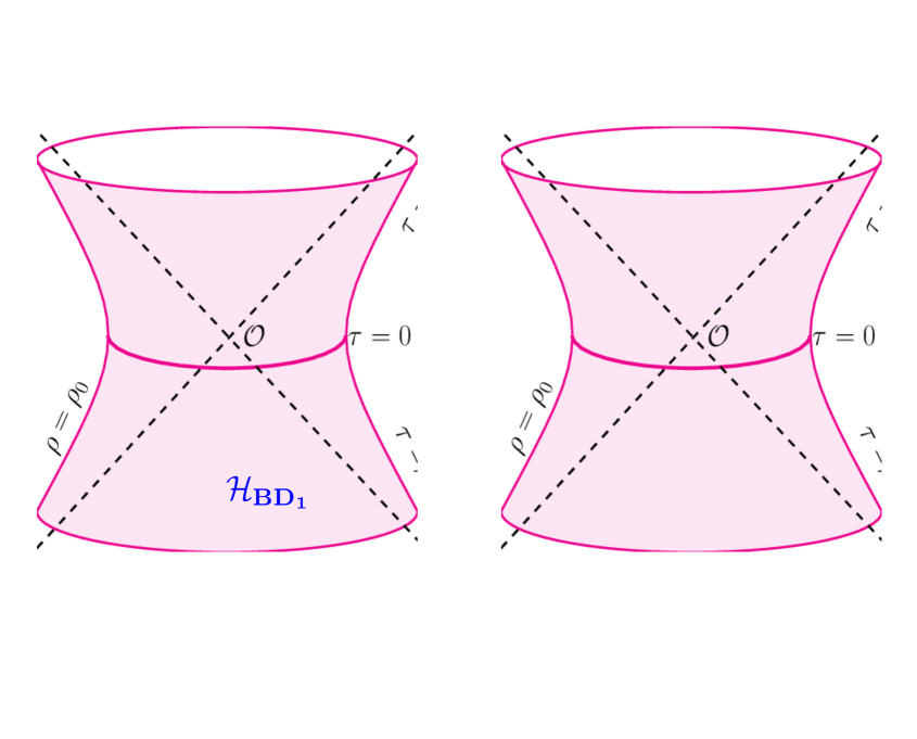
To compute the reduced density matrix as well as the mentioned quantum information theoretic measures we need to first of all understand the underlying quantum field theoretic set up in detail. To serve the purpose we need to first of all understand the Hilbert space structure of the open chart of global de Sitter space. This would be also helpful to implement the two causally unrelated patches of the open charts in terms of the quantum mechanical Hilbert space. In this construction let us first of all consider a closed surface ΣΣ\displaystyle\Sigma in a space like hypersurface. As an outcome of this fact, this hypersurface can be visualized in terms of an exterior and an interior region. For further simplification purpose we identify the interior region as RI, which is tagged with 𝐋𝐋{\bf L} region the associated Penrose diagram presented in figure (3.1). Similarly, the exterior region is identified as RII, which is the 𝐑𝐑{\bf R} region in the corresponding diagram. By looking at the geometrical structure of the two causally unrelated patches of the open chart it is expected that the representative quantum field theory has to be bipartite, which will suffice the purpose for the quantum mechanical construction of the corresponding set up. To describe this set up let us consider the fact that the Hilbert space of the total system is described by {\bf\cal H}. Then for the bipartite quantum set up the total Hilbert space {\bf\cal H} can be decomposed in terms of the tensor products of two Hilbert spaces associated with the tagged 𝐋𝐋{\bf L} and 𝐑𝐑{\bf R} region, as described above. Technically this is written as, =𝐋𝐑.tensor-productsubscript𝐋subscript𝐑{\bf\cal H}={\bf\cal H}_{\bf L}\otimes{\bf\cal H}_{\bf R}. Here 𝐋subscript𝐋{\bf\cal H}_{\bf L} and 𝐑subscript𝐑{\bf\cal H}_{\bf R} represent the corresponding Hilbert spaces of the subsystems 𝐋𝐋{\bf L} and 𝐑𝐑{\bf R} respectively. This is perfectly consistent with the local description of quantum field theory. However, in the more generalized description, it might not always true that in the underlying quantum theory the total Hilbert space can be factorized very easily and can be written in terms of tensor products of the subsystem Hilbert spaces. This is because of the fact that the underlying physical theory might not be bipartite in nature. Dealing with this type of physical systems at the level of computation is extremely difficult to handle. To handle such systems at the level of analysis sometimes the concept of short distance lattice cut-off is introduced within the framework of quantum field theory, which actually perfectly allows the bipartite construction in the computational set up. Additionally, it is important to note that, in this construction the localized modes play significant role to construct the building blocks of tagged 𝐋𝐋{\bf L} and 𝐑𝐑{\bf R} regions respectively. Consequently, this quantum mechanical formulation allows us to construct the expression for the reduced density matrix of the region 𝐋𝐋{\bf L} by tracing out all the information of the region 𝐑𝐑{\bf R}. Similar argument holds for the construction of density matrix for the region 𝐑𝐑{\bf R}. In our computation, we assume that the region 𝐑𝐑{\bf R} and the region 𝐋𝐋{\bf L} are the replica or identical copy of each other. For this reason constructing any one of the reduced density matrix is sufficient enough to describe the subsystem in the present context of discussion. Here the reduced density matrix can be written as:

ρ𝐋=Tr𝐑(|Ψ𝐁𝐃Ψ𝐁𝐃|).subscript𝜌𝐋subscriptTr𝐑ketsubscriptΨ𝐁𝐃brasubscriptΨ𝐁𝐃\displaystyle\rho_{\bf L}={\rm Tr}_{\bf R}\left(|\Psi_{\bf BD}\rangle\langle\Psi_{\bf BD}|\right). (3.1)

Here the underlying initial quantum vacuum structure is characterized in terms of the state vector |Ψ𝐁𝐃ketsubscriptΨ𝐁𝐃|\Psi_{\bf BD}\rangle, commonly known as the Bunch-Davies vacuum. Now from the above mentioned expression it is quite obvious that if we can able to construct the mathematical structure of the Bunch-Davies vacuum state vector in the mentioned Hilbert space, then we can immediately compute the expression for the reduced density matrix, using which one can further derive the expressions for entanglement entropy measures, von Neumann and Renyi, entanglement negativity and logarithmic negativity. Now the prime point at this stage is to fix the structure of the initial quantum vacuum state vector one need to know the geometrical structure of the background space time, which is open chart of global de Sitter space and also about the explicit matter content which is embedded in the mentioned space time. In our case, we will embed string theory originated axion field as a scalar matter on the mentioned space time, which will going to help us to explicitly compute the mode functions in open chart. Once the mode functions are computed as a function of momentum and various quantum numbers, then the specific structure of the Bunch-Davies vacuum state vector can be fixed from the present computational algorithm. In the next subsection we elaborately discuss the geometrical structure of the open chart of the global de Sitter space time, which we believe will going to extremely helpful to underlying technical construction of the physical problem that we are studying in this paper.

3.2 Geometric structure of open chart
Refer to caption
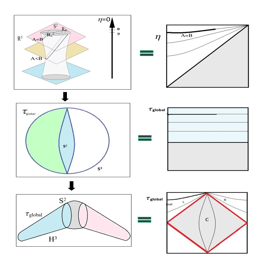
Figure 3.1: Representative diagram and penrose diagram for the geometrical construction of the bipartite system.

In this subsection we are going to discuss about the geometrical structure of open chart in global de Sitter space time. Let us consider a surface of two sphere (𝐒2superscript𝐒2{\bf S}^{2}) whose geometry is described by the following equation:

i=13xi2=R2,subscriptsuperscript3𝑖1subscriptsuperscript𝑥2𝑖superscript𝑅2\displaystyle\sum^{3}_{i=1}x^{2}_{i}=R^{2}, (3.2)

where R𝑅R is the radius of the two sphere and xii=1,2,3subscript𝑥𝑖for-all𝑖123x_{i}\forall i=1,2,3 represent three orthogonal coordinates. For the practical purpose here we need to consider that the radius of the two sphere is sufficiently large enough compared to the horizon size. Now since the horizon size is described by the conformal time scale, then here we need Rτmuch-greater-than𝑅𝜏R\gg\tau, where τ𝜏\tau represents the conformal time. In practical purposes this can be achieved by taking the late time limit τ0𝜏0\tau\rightarrow 0. Here it is important to note that the surface of the two sphere that we are discussing in this section is invariant under the 𝐒𝐎(𝟏,𝟑)𝐒𝐎13{\rm\bf SO(1,3)} transformation. In this construction the actual symmetry group is 𝐒𝐎(𝟏,𝟒)𝐒𝐎14{\rm\bf SO(1,4)}, which is known as the isometry group of de Sitter space and 𝐒𝐎(𝟏,𝟑)𝐒𝐎13{\rm\bf SO(1,3)} forms a subgroup of this bigger isometry group. In the representative penrose diagram this particular geometry is appearing in the tagged left region as shown in figure (3.1). In our computation we choose equal conformal time slice on three sphere 𝐒3superscript𝐒3{\bf S}^{3}, which is appearing in the context of the global coordinates of de Sitter space. Most importantly, it is noted that the surface of two sphere is treated to be the equator of the three sphere in this geometrical construction. This conformal map on the boundary of 3+1313+1 dimensional global de Sitter space effectively produce divergent contributions, which can be easily regulated by taking another conformal reverse map from three sphere to two sphere via a global time surface.

Further, we consider the following 1+4141+4 dimensional Euclidean global hyperbolic geometry which is defined as:

𝐄𝐮𝐜𝐥𝐢𝐝𝐞𝐚𝐧𝐠𝐥𝐨𝐛𝐚𝐥𝐡𝐲𝐩𝐞𝐫𝐛𝐨𝐥𝐢𝐜𝐠𝐞𝐨𝐦𝐞𝐭𝐫𝐲:j=15Yj2=1H2,:𝐄𝐮𝐜𝐥𝐢𝐝𝐞𝐚𝐧𝐠𝐥𝐨𝐛𝐚𝐥𝐡𝐲𝐩𝐞𝐫𝐛𝐨𝐥𝐢𝐜𝐠𝐞𝐨𝐦𝐞𝐭𝐫𝐲subscriptsuperscript5𝑗1subscriptsuperscript𝑌2𝑗1superscript𝐻2\displaystyle{\bf Euclidean\leavevmode\nobreak\ global\leavevmode\nobreak\ hyperbolic\leavevmode\nobreak\ geometry:\Longrightarrow}\quad\quad\quad\sum^{5}_{j=1}Y^{2}_{j}=\frac{1}{H^{2}}, (3.3)

where the corresponding 1+4141+4 dimensional coordinates are given by the following equation:

Yjsubscript𝑌𝑗\displaystyle\displaystyle Y_{j} =\displaystyle= 1H×{cosτ𝐄sinσ𝐄𝐧^jfor j=1,2,3sinτ𝐄 for j=4cosτ𝐄cosσ𝐄 for j=5.1𝐻casessubscript𝜏𝐄subscript𝜎𝐄subscript^𝐧𝑗for j=1,2,3subscript𝜏𝐄 for j=4subscript𝜏𝐄subscript𝜎𝐄 for j=5\displaystyle\displaystyle\frac{1}{H}\times\left\{\begin{array}[]{ll}\displaystyle\cos\tau_{\bf E}\leavevmode\nobreak\ \sin\sigma_{\bf E}\leavevmode\nobreak\ \hat{\bf n}_{j}\nobreak\leavevmode\nobreak\leavevmode\nobreak\leavevmode\nobreak\leavevmode\nobreak\leavevmode\nobreak\leavevmode\nobreak\leavevmode\nobreak\leavevmode\nobreak\leavevmode\nobreak\leavevmode\nobreak\leavevmode\nobreak\leavevmode&\mbox{\small{{\color[rgb]{0,0,0}\definecolor[named]{pgfstrokecolor}{rgb}{0,0,0}\pgfsys@color@gray@stroke{0}\pgfsys@color@gray@fill{0}\bf for $j=1,2,3$}}}\\ \displaystyle\sin\tau_{\bf E}&\mbox{\small{ {\color[rgb]{0,0,0}\definecolor[named]{pgfstrokecolor}{rgb}{0,0,0}\pgfsys@color@gray@stroke{0}\pgfsys@color@gray@fill{0}\bf for $j=4$}}}\\ \displaystyle\cos\tau_{\bf E}\leavevmode\nobreak\ \cos\sigma_{\bf E}&\mbox{\small{ {\color[rgb]{0,0,0}\definecolor[named]{pgfstrokecolor}{rgb}{0,0,0}\pgfsys@color@gray@stroke{0}\pgfsys@color@gray@fill{0}\bf for $j=5$}}}.\nobreak\leavevmode\nobreak\leavevmode\nobreak\leavevmode\nobreak\leavevmode\nobreak\leavevmode\nobreak\leavevmode\nobreak\leavevmode\nobreak\leavevmode\end{array}\right. (3.7)

Here 𝐧^jj=1,2,3subscript^𝐧𝑗for-all𝑗123\hat{\bf n}_{j}\forall j=1,2,3 are the three components which is in 𝐑3superscript𝐑3{\bf R}^{3}. The corresponding Euclidean metric is is given by:

𝐋𝐨𝐫𝐞𝐧𝐭𝐳𝐢𝐚𝐧𝐦𝐞𝐭𝐫𝐢𝐜:ds𝐄2=1H2{dτ𝐄2+cos2τ𝐄(dσ𝐄2+sin2σ𝐄dΩ𝟐2)},:𝐋𝐨𝐫𝐞𝐧𝐭𝐳𝐢𝐚𝐧𝐦𝐞𝐭𝐫𝐢𝐜𝑑subscriptsuperscript𝑠2𝐄1superscript𝐻2𝑑subscriptsuperscript𝜏2𝐄superscript2subscript𝜏𝐄𝑑subscriptsuperscript𝜎2𝐄superscript2subscript𝜎𝐄𝑑subscriptsuperscriptΩ22\displaystyle{\bf Lorentzian\leavevmode\nobreak\ metric:\Longrightarrow}\quad\quad\quad ds^{2}_{\bf E}=\frac{1}{H^{2}}\left\{d\tau^{2}_{\bf E}+\cos^{2}\tau_{\bf E}\left(d\sigma^{2}_{\bf E}+\sin^{2}\sigma_{\bf E}\leavevmode\nobreak\ d\Omega^{2}_{\bf 2}\right)\right\}, (3.8)

where dΩ𝟐2𝑑subscriptsuperscriptΩ22d\Omega^{2}_{\bf 2} is the line element in two sphere. Now we take analytic continuation in the fifth coordinate, which gives:

Y5=1Hcosτ𝐄cosσ𝐄𝐀𝐧𝐚𝐥𝐲𝐭𝐢𝐜𝐜𝐨𝐧𝐭𝐢𝐧𝐮𝐚𝐭𝐢𝐨𝐧𝐗𝟎=𝐢𝐘𝟓=𝐢𝐇cosτ𝐄cosσ𝐄subscript𝑌51𝐻subscript𝜏𝐄subscript𝜎𝐄𝐀𝐧𝐚𝐥𝐲𝐭𝐢𝐜𝐜𝐨𝐧𝐭𝐢𝐧𝐮𝐚𝐭𝐢𝐨𝐧subscript𝐗0subscript𝐢𝐘5𝐢𝐇subscript𝜏𝐄subscript𝜎𝐄\displaystyle Y_{5}=\frac{1}{H}\cos\tau_{\bf E}\leavevmode\nobreak\ \cos\sigma_{\bf E}\xrightarrow[]{\bf Analytic\leavevmode\nobreak\ continuation}X_{0}=iY_{5}=\frac{i}{H}\cos\tau_{\bf E}\leavevmode\nobreak\ \cos\sigma_{\bf E} (3.9)

and consider the coordinate redefinition of the part, which give rise to:

𝐑𝐞𝐝𝐞𝐟𝐢𝐧𝐞𝐝𝐜𝐨𝐨𝐫𝐝𝐢𝐧𝐚𝐭𝐞𝐬:Xk=Ykk=1,2,3,4.\displaystyle{\bf Redefined\leavevmode\nobreak\ coordinates:\Longrightarrow}\quad\quad\quad X_{k}=Y_{k}\leavevmode\nobreak\ \leavevmode\nobreak\ \leavevmode\nobreak\ \leavevmode\nobreak\ \leavevmode\nobreak\ \leavevmode\nobreak\ \leavevmode\nobreak\ \leavevmode\nobreak\ \leavevmode\nobreak\ {\forall k=1,2,3,4}. (3.10)

As a result, the corresponding Lorentzian geometry is described by the following representative equation:

𝐋𝐨𝐫𝐞𝐧𝐭𝐳𝐢𝐚𝐧𝐠𝐞𝐨𝐦𝐞𝐭𝐫𝐲:1H2=μ=04Xμ2=(X02+j=14Xj2).:𝐋𝐨𝐫𝐞𝐧𝐭𝐳𝐢𝐚𝐧𝐠𝐞𝐨𝐦𝐞𝐭𝐫𝐲1superscript𝐻2subscriptsuperscript4𝜇0subscriptsuperscript𝑋2𝜇subscriptsuperscript𝑋20subscriptsuperscript4𝑗1subscriptsuperscript𝑋2𝑗\displaystyle{\bf Lorentzian\leavevmode\nobreak\ geometry:\Longrightarrow}\quad\quad\quad\frac{1}{H^{2}}=\sum^{4}_{\mu=0}X^{2}_{\mu}=\left(-X^{2}_{0}+\sum^{4}_{j=1}X^{2}_{j}\right). (3.11)

Since we have transformed the coordinate in Lorentzian signature, the corresponding Lorentzian geometry for the different regions in the representative penrose diagram is described by the following coordinates:

𝐑𝐞𝐠𝐢𝐨𝐧𝐑𝐑𝐞𝐠𝐢𝐨𝐧𝐑\displaystyle\displaystyle{\color[rgb]{0,0,0}\definecolor[named]{pgfstrokecolor}{rgb}{0,0,0}\pgfsys@color@gray@stroke{0}\pgfsys@color@gray@fill{0}\bf Region-R} ::absent\displaystyle:\Longrightarrow {τ𝐄=π2it𝐑for t𝐑0σ𝐄=ir𝐑 for rR0.casessubscript𝜏𝐄𝜋2𝑖subscript𝑡𝐑for t𝐑0subscript𝜎𝐄𝑖subscript𝑟𝐑 for rR0\displaystyle\displaystyle\left\{\begin{array}[]{ll}\displaystyle\tau_{\bf E}=\frac{\pi}{2}-it_{\bf R}\nobreak\leavevmode\nobreak\leavevmode\nobreak\leavevmode\nobreak\leavevmode\nobreak\leavevmode\nobreak\leavevmode\nobreak\leavevmode\nobreak\leavevmode\nobreak\leavevmode\nobreak\leavevmode\nobreak\leavevmode\nobreak\leavevmode&\mbox{\small{{\color[rgb]{0,0,0}\definecolor[named]{pgfstrokecolor}{rgb}{0,0,0}\pgfsys@color@gray@stroke{0}\pgfsys@color@gray@fill{0}\bf for $t_{\bf R}\geq 0$}}}\\ \displaystyle\sigma_{\bf E}=-ir_{\bf R}&\mbox{\small{ {\color[rgb]{0,0,0}\definecolor[named]{pgfstrokecolor}{rgb}{0,0,0}\pgfsys@color@gray@stroke{0}\pgfsys@color@gray@fill{0}\bf for $r_{\bf R}\geq 0$}}}.\nobreak\leavevmode\nobreak\leavevmode\nobreak\leavevmode\nobreak\leavevmode\nobreak\leavevmode\nobreak\leavevmode\nobreak\leavevmode\nobreak\leavevmode\end{array}\right. (3.14)
𝐑𝐞𝐠𝐢𝐨𝐧𝐂𝐑𝐞𝐠𝐢𝐨𝐧𝐂\displaystyle\displaystyle{\color[rgb]{0,0,0}\definecolor[named]{pgfstrokecolor}{rgb}{0,0,0}\pgfsys@color@gray@stroke{0}\pgfsys@color@gray@fill{0}\bf Region-C} ::absent\displaystyle:\Longrightarrow {τ𝐄=t𝐂for π2t𝐂π2σ𝐄=π2ir𝐂 for <rC<.casessubscript𝜏𝐄subscript𝑡𝐂for π2t𝐂π2subscript𝜎𝐄𝜋2𝑖subscript𝑟𝐂 for <rC<\displaystyle\displaystyle\left\{\begin{array}[]{ll}\displaystyle\tau_{\bf E}=t_{\bf C}\nobreak\leavevmode\nobreak\leavevmode\nobreak\leavevmode\nobreak\leavevmode\nobreak\leavevmode\nobreak\leavevmode\nobreak\leavevmode\nobreak\leavevmode\nobreak\leavevmode\nobreak\leavevmode\nobreak\leavevmode\nobreak\leavevmode\nobreak\leavevmode\nobreak\leavevmode\nobreak\leavevmode\nobreak\leavevmode\nobreak\leavevmode\nobreak\leavevmode&\mbox{\small{{\color[rgb]{0,0,0}\definecolor[named]{pgfstrokecolor}{rgb}{0,0,0}\pgfsys@color@gray@stroke{0}\pgfsys@color@gray@fill{0}\bf for $\displaystyle-\frac{\pi}{2}\leq t_{\bf C}\leq\frac{\pi}{2}$}}}\\ \displaystyle\sigma_{\bf E}=\frac{\pi}{2}-ir_{\bf C}&\mbox{\small{ {\color[rgb]{0,0,0}\definecolor[named]{pgfstrokecolor}{rgb}{0,0,0}\pgfsys@color@gray@stroke{0}\pgfsys@color@gray@fill{0}\bf for $-\infty<r_{\bf C}<\infty$}}}.\nobreak\leavevmode\nobreak\leavevmode\nobreak\leavevmode\nobreak\leavevmode\nobreak\leavevmode\nobreak\leavevmode\nobreak\leavevmode\nobreak\leavevmode\nobreak\leavevmode\nobreak\leavevmode\nobreak\leavevmode\nobreak\leavevmode\nobreak\leavevmode\nobreak\leavevmode\end{array}\right. (3.17)
𝐑𝐞𝐠𝐢𝐨𝐧𝐋𝐑𝐞𝐠𝐢𝐨𝐧𝐋\displaystyle\displaystyle{\color[rgb]{0,0,0}\definecolor[named]{pgfstrokecolor}{rgb}{0,0,0}\pgfsys@color@gray@stroke{0}\pgfsys@color@gray@fill{0}\bf Region-L} ::absent\displaystyle:\Longrightarrow {τ𝐄=π2+it𝐋 for tL0σ𝐄=ir𝐋 for rL0.casessubscript𝜏𝐄𝜋2𝑖subscript𝑡𝐋 for tL0subscript𝜎𝐄𝑖subscript𝑟𝐋 for rL0\displaystyle\displaystyle\left\{\begin{array}[]{ll}\displaystyle\tau_{\bf E}=-\frac{\pi}{2}+it_{\bf L}\nobreak\leavevmode\nobreak\leavevmode\nobreak\leavevmode\nobreak\leavevmode\nobreak\leavevmode\nobreak\leavevmode\nobreak\leavevmode\nobreak\leavevmode\nobreak\leavevmode\nobreak\leavevmode\nobreak\leavevmode\nobreak\leavevmode&\mbox{\small{ {\color[rgb]{0,0,0}\definecolor[named]{pgfstrokecolor}{rgb}{0,0,0}\pgfsys@color@gray@stroke{0}\pgfsys@color@gray@fill{0}\bf for $t_{\bf L}\geq 0$}}}\\ \displaystyle\sigma_{\bf E}=-ir_{\bf L}&\mbox{\small{ {\color[rgb]{0,0,0}\definecolor[named]{pgfstrokecolor}{rgb}{0,0,0}\pgfsys@color@gray@stroke{0}\pgfsys@color@gray@fill{0}\bf for $r_{\bf L}\geq 0$}}}.\nobreak\leavevmode\nobreak\leavevmode\nobreak\leavevmode\nobreak\leavevmode\nobreak\leavevmode\nobreak\leavevmode\nobreak\leavevmode\nobreak\leavevmode\end{array}\right. (3.20)

Finally, the representative Lorentzian metric for the three different regions, as mentioned above can be written as [1, 13, 19, 14, 15, 16]:

𝐑𝐞𝐠𝐢𝐨𝐧𝐑𝐑𝐞𝐠𝐢𝐨𝐧𝐑\displaystyle\displaystyle{\color[rgb]{0,0,0}\definecolor[named]{pgfstrokecolor}{rgb}{0,0,0}\pgfsys@color@gray@stroke{0}\pgfsys@color@gray@fill{0}\bf Region-R} ::absent\displaystyle:\Longrightarrow {ds𝐑2=1H2[dt𝐑2+sinh2t𝐑(dr𝐑2+sinh2r𝐑dΩ𝟐2)],cases𝑑subscriptsuperscript𝑠2𝐑1superscript𝐻2delimited-[]𝑑subscriptsuperscript𝑡2𝐑superscript2subscript𝑡𝐑𝑑subscriptsuperscript𝑟2𝐑superscript2subscript𝑟𝐑𝑑subscriptsuperscriptΩ22missing-subexpression\displaystyle\displaystyle\left\{\begin{array}[]{ll}\displaystyle ds^{2}_{\bf R}=\frac{1}{H^{2}}\left[-dt^{2}_{\bf R}+\sinh^{2}t_{\bf R}\left(dr^{2}_{\bf R}+\sinh^{2}r_{\bf R}\leavevmode\nobreak\ d\Omega^{2}_{\bf 2}\right)\right],\end{array}\right. (3.22)
𝐑𝐞𝐠𝐢𝐨𝐧𝐂𝐑𝐞𝐠𝐢𝐨𝐧𝐂\displaystyle\displaystyle{\color[rgb]{0,0,0}\definecolor[named]{pgfstrokecolor}{rgb}{0,0,0}\pgfsys@color@gray@stroke{0}\pgfsys@color@gray@fill{0}\bf Region-C} ::absent\displaystyle:\Longrightarrow {ds𝐂2=1H2[dt𝐂2+cos2t𝐂(dr𝐂2+cosh2r𝐂dΩ𝟐2)],cases𝑑subscriptsuperscript𝑠2𝐂1superscript𝐻2delimited-[]𝑑subscriptsuperscript𝑡2𝐂superscript2subscript𝑡𝐂𝑑subscriptsuperscript𝑟2𝐂superscript2subscript𝑟𝐂𝑑subscriptsuperscriptΩ22missing-subexpression\displaystyle\displaystyle\left\{\begin{array}[]{ll}\displaystyle ds^{2}_{\bf C}=\frac{1}{H^{2}}\left[dt^{2}_{\bf C}+\cos^{2}t_{\bf C}\left(-dr^{2}_{\bf C}+\cosh^{2}r_{\bf C}\leavevmode\nobreak\ d\Omega^{2}_{\bf 2}\right)\right],\end{array}\right. (3.24)
𝐑𝐞𝐠𝐢𝐨𝐧𝐋𝐑𝐞𝐠𝐢𝐨𝐧𝐋\displaystyle\displaystyle{\color[rgb]{0,0,0}\definecolor[named]{pgfstrokecolor}{rgb}{0,0,0}\pgfsys@color@gray@stroke{0}\pgfsys@color@gray@fill{0}\bf Region-L} ::absent\displaystyle:\Longrightarrow {ds𝐋2=1H2[dt𝐋2+sinh2t𝐋(dr𝐋2+sinh2r𝐋dΩ𝟐2)].cases𝑑subscriptsuperscript𝑠2𝐋1superscript𝐻2delimited-[]𝑑subscriptsuperscript𝑡2𝐋superscript2subscript𝑡𝐋𝑑subscriptsuperscript𝑟2𝐋superscript2subscript𝑟𝐋𝑑subscriptsuperscriptΩ22missing-subexpression\displaystyle\displaystyle\left\{\begin{array}[]{ll}\displaystyle ds^{2}_{\bf L}=\frac{1}{H^{2}}\left[-dt^{2}_{\bf L}+\sinh^{2}t_{\bf L}\left(dr^{2}_{\bf L}+\sinh^{2}r_{\bf L}\leavevmode\nobreak\ d\Omega^{2}_{\bf 2}\right)\right].\end{array}\right. (3.26)
Refer to caption
(a) For 𝐋𝐋{\bf L} and 𝐑𝐑{\bf R}.
Refer to caption
(b) For 𝐂𝐂{\bf C}.
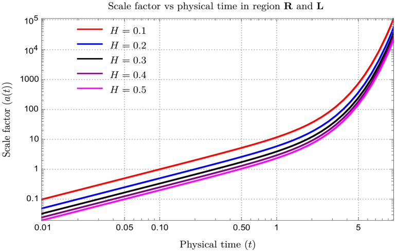
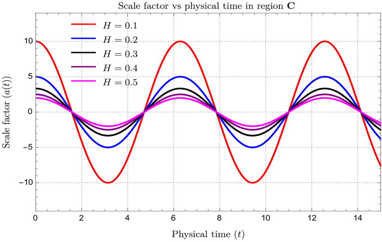
Figure 3.2: Graphical behaviour of the scale factor (a(t)𝑎𝑡a(t)) with respect to physical time (t𝑡t) in the region L, R and C of the penrose diagram.

Here the scale factor a(t)𝑎𝑡a(t) in the three regions in terms of physical time variable t𝑡t can be written as:

𝐑𝐞𝐠𝐢𝐨𝐧𝐑𝐑𝐞𝐠𝐢𝐨𝐧𝐑\displaystyle\displaystyle{\color[rgb]{0,0,0}\definecolor[named]{pgfstrokecolor}{rgb}{0,0,0}\pgfsys@color@gray@stroke{0}\pgfsys@color@gray@fill{0}\bf Region-R} ::absent\displaystyle:\Longrightarrow {a(t𝐑)=1Hsinht𝐑,cases𝑎subscript𝑡𝐑1𝐻subscript𝑡𝐑missing-subexpression\displaystyle\displaystyle\left\{\begin{array}[]{ll}\displaystyle a(t_{\bf R})=\frac{1}{H}\sinh t_{\bf R},\end{array}\right. (3.28)
𝐑𝐞𝐠𝐢𝐨𝐧𝐂𝐑𝐞𝐠𝐢𝐨𝐧𝐂\displaystyle\displaystyle{\color[rgb]{0,0,0}\definecolor[named]{pgfstrokecolor}{rgb}{0,0,0}\pgfsys@color@gray@stroke{0}\pgfsys@color@gray@fill{0}\bf Region-C} ::absent\displaystyle:\Longrightarrow {a(t𝐂)=1Hcost𝐂,cases𝑎subscript𝑡𝐂1𝐻subscript𝑡𝐂missing-subexpression\displaystyle\displaystyle\left\{\begin{array}[]{ll}\displaystyle a(t_{\bf C})=\frac{1}{H}\cos t_{\bf C},\end{array}\right. (3.30)
𝐑𝐞𝐠𝐢𝐨𝐧𝐋𝐑𝐞𝐠𝐢𝐨𝐧𝐋\displaystyle\displaystyle{\color[rgb]{0,0,0}\definecolor[named]{pgfstrokecolor}{rgb}{0,0,0}\pgfsys@color@gray@stroke{0}\pgfsys@color@gray@fill{0}\bf Region-L} ::absent\displaystyle:\Longrightarrow {a(t𝐋)=1Hsinht𝐋cases𝑎subscript𝑡𝐋1𝐻subscript𝑡𝐋missing-subexpression\displaystyle\displaystyle\left\{\begin{array}[]{ll}\displaystyle a(t_{\bf L})=\frac{1}{H}\sinh t_{\bf L}\end{array}\right. (3.32)

Here H𝐻H is Hubble parameter which is treated to be a constant in the above mentioned three regions of consideration. In figure (3.2(a)) and figure (3.2(b)) we have plotted the behaviour of the scale factor a(t)𝑎𝑡a(t) with respect to the physical time scale t𝑡t in regions R, R and C respectively. From the plots its clearly observed that in the case of region L and R the behaviour is same and show growing behaviour with respect to time. This is expected from the geometrical construction global de Sitter space. On the other hand, for the region C it shows periodic oscillatory behaviour. In all of these plots we have used different values of the Hubble constants in dimensionless units.

In the next subsection, we will compute the expression for the wave function in presence of string theory originated axion effective interactions either in the region L or R of the open chart of the hyperbolic slices of global de Sitter space. According to our construction of the geometrical set up the region L and R are replica of each other and exactly symmetric, which can easily be observed from the representative pensore diagram as shown in figure (3.1). For this particular reason we derive the wave function in both the regions, but taking the partial trace over the contributions of the region R, we use only the effective contributions from the region L during the construction of reduced density matrix. The similar trick can be applicable to the region R as well.

3.3 Mode function and wave function of axion in an open chart

In this part, we compute the equations for the global de Sitter space time hyperbolic open chart’s hyperbolic open mode functions, associated wave functions, and quantum number and momentum dependent mode functions. We use the string theory-derived axion effective potential, which manifests as a scalar field in the matter sector, to make it happen. This outcome will be very helpful in computing the decreased density matrix expression as well as the entanglement negativity and its logarithmic counterpart in the following subsection. It is crucial to emphasise that in the current discussion, we are interested in the axion monodromy model.

In the present construction the axion field is generated from RR𝑅𝑅RR sector of the Type IIB string theory set up, where the effective potential and the related interaction is originated as an outcome of the compactification on a Calabi-Yau three fold in presence of NS5𝑁𝑆5NS5 brane. For the details from the string theory construction of the present set up see the refs. [48, 49, 50] for the better understanding on the subject and the model we are considering in our paper. We have mentioned clearly in the introductory part of this paper that, axion would be the best candidate to study the effects of CHSH version of Bell’s inequality violation. For this reason the computational outcomes of this section will going to help us to study the non-local effects of quantum mechanical entanglement, which is necessarily required to violate Bell’s inequality from the quantum information theoretic point of view. One important fact we need to explicitly point out that, in the context of bipartite quantum field theoretic set up explicit violation of Bell’s CHSH inequality necessarily requires the existence of quantum mechanical entanglement in the prescribed theoretical set up. But the converse fact is not always necessarily true. Regarding this exception see ref. [31] which will give a clear underlying physical idea of the mentioned fact. In this description the specific theoretical structure of the quantum mechanical state play very significant role. Because within the framework quantum information theory bipartite system is characterised by a specific type of quantum state, commonly known as Werner type of states which produce non zero quantum entanglement measure and this is the most important underlying concept to connect with the Bell’s CHSH inequality violation [31]. But the underlying behaviour of such states are not very clear in the present framework and without knowing the details it is very complicated to pursue the present analysis.
Refer to caption
(a) For b<0𝑏0b<0
Refer to caption
(b) For b>0𝑏0b>0
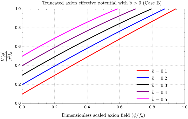
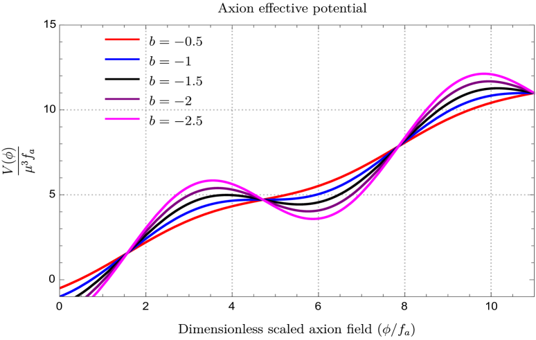
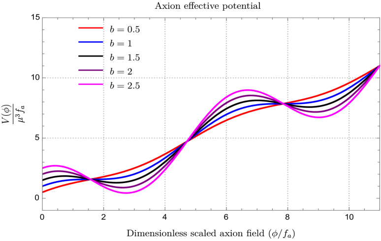
Figure 3.3: Graphical behaviour of the axion effective potential with respect to the field obtained from Type IIB String Theory compactification for stringy parameter b<0𝑏0b<0 and b>0𝑏0b>0.

Let us start with the following canonical effective action for axion field minimally coupled with the gravitational sector by space-time metric in 1+3131+3 dimensions:

𝐄𝐟𝐟𝐞𝐜𝐭𝐢𝐯𝐞𝐚𝐜𝐭𝐢𝐨𝐧:S=d4xg[12(ϕ)2V(ϕ)],{\bf Effective\leavevmode\nobreak\ action:}\leavevmode\nobreak\ \leavevmode\nobreak\ \leavevmode\nobreak\ \leavevmode\nobreak\ \leavevmode\nobreak\ S=\int d^{4}x\sqrt{-g}\left[-\frac{1}{2}(\partial\phi)^{2}-V(\phi)\right], (3.33)

This action is derived from string compactification and is extremely useful to study the quntum information theoretic measures related to quantum entanglement. Here ϕitalic-ϕ\phi is the dimensionful axionic field, which is described by the following effective potential [48, 49, 50] :

𝐄𝐟𝐟𝐞𝐜𝐭𝐢𝐯𝐞𝐩𝐨𝐭𝐞𝐧𝐭𝐢𝐚𝐥:V(ϕ)\displaystyle{\bf Effective\leavevmode\nobreak\ potential:}\leavevmode\nobreak\ \leavevmode\nobreak\ \leavevmode\nobreak\ \leavevmode\nobreak\ \leavevmode\nobreak\ V(\phi) =\displaystyle= μ3ϕ+ΛG4cos(ϕfa)superscript𝜇3italic-ϕsubscriptsuperscriptΛ4𝐺italic-ϕsubscript𝑓𝑎\displaystyle\mu^{3}\phi+\Lambda^{4}_{G}\cos\left(\frac{\phi}{f_{a}}\right) (3.34)
=\displaystyle= μ3fa[(ϕfa)+bcos(ϕfa)].superscript𝜇3subscript𝑓𝑎delimited-[]italic-ϕsubscript𝑓𝑎𝑏italic-ϕsubscript𝑓𝑎\displaystyle\mu^{3}f_{a}\left[\left(\frac{\phi}{f_{a}}\right)+b\cos\left(\frac{\phi}{f_{a}}\right)\right].\leavevmode\nobreak\ \leavevmode\nobreak\ \leavevmode\nobreak\ \leavevmode\nobreak\ \leavevmode\nobreak\ \leavevmode\nobreak\ \leavevmode\nobreak\ \leavevmode\nobreak\ \leavevmode\nobreak\ \leavevmode\nobreak\
Refer to caption
(a) For conformal time
Refer to caption
(b) For physical time
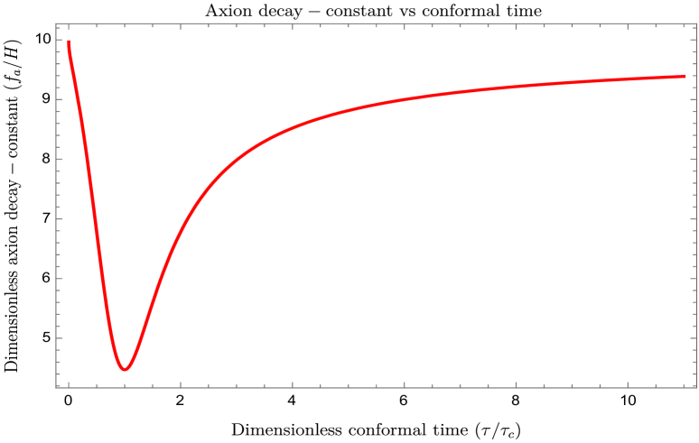
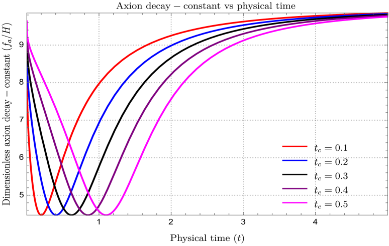
Figure 3.4: Schematic behaviour of the dimensionless axion decay constant with the conformal and physical time scale.

In figure (3.3(a)) and figure (3.3(b)) we have plotted the behaviour of the dimensionless axion effective potential V(ϕ)/μ3fa𝑉italic-ϕsuperscript𝜇3subscript𝑓𝑎V(\phi)/\mu^{3}f_{a} with respect to the dimensionless axion field variable ϕ/faitalic-ϕsubscript𝑓𝑎\phi/f_{a} for the stringy parameter b>0𝑏0b>0 and b>0𝑏0b>0. The precise definition of the stringy parameter b𝑏b is written in the later part of this paper explicitly. Both the behaviour are useful to understand the contribution of the linear and non-perterbative periodic part in the total axion effective potential.

In this effective potential μ3superscript𝜇3\mu^{3} represents the coupling parameter of linear interaction which is associated with the underlying theoretical scale, can be expressed as:

𝐒𝐜𝐚𝐥𝐞𝐨𝐟𝐞𝐟𝐟𝐞𝐜𝐭𝐢𝐯𝐞𝐩𝐨𝐭𝐞𝐧𝐭𝐢𝐚𝐥:μ3=1faα2gsexp(4A0)+R2mSUSY4faαL4exp(2A0),\displaystyle{\bf Scale\leavevmode\nobreak\ of\leavevmode\nobreak\ effective\leavevmode\nobreak\ potential:}\leavevmode\nobreak\ \leavevmode\nobreak\ \leavevmode\nobreak\ \leavevmode\nobreak\ \leavevmode\nobreak\ \mu^{3}=\frac{1}{f_{a}\alpha^{{}^{\prime}2}g_{s}}\exp(4A_{0})+\frac{R^{2}m^{4}_{SUSY}}{f_{a}\alpha^{{}^{\prime}}L^{4}}\exp(2A_{0}),\leavevmode\nobreak\ \leavevmode\nobreak\ \leavevmode\nobreak\ \leavevmode\nobreak\ \leavevmode\nobreak\ (3.35)

where exp(A0)subscript𝐴0\exp(A_{0}) represents the warp factor of the lower portion of the Klebanov-Strassler throat geometry, R𝑅R is the radius which stabilized the 555 brane and antibrane in the corresponding string theory construction, the only mass scale involved in this construction is mSUSYsubscript𝑚𝑆𝑈𝑆𝑌m_{SUSY}, which actually represents the underlying supersymmetry breaking scale in this specific set up, the Regge slope is αsuperscript𝛼\alpha^{{}^{\prime}} which is proportional to the inverse string tension, string coupling is gssubscript𝑔𝑠g_{s} and finally L6superscript𝐿6L^{6} represents the world volume. Here first part of the effective potential breaks the shift symmetry and the rest of the part preserves the symmetry ϕϕ+2πfaitalic-ϕitalic-ϕ2𝜋subscript𝑓𝑎\phi\rightarrow\phi+2\pi f_{a}. Here fasubscript𝑓𝑎f_{a} quantifies the axionic decay parameter, which is in general conformal time dependent (τ𝜏\tau) and we have chosen the following useful profile:

𝐀𝐱𝐢𝐨𝐧𝐝𝐞𝐜𝐚𝐲𝐜𝐨𝐧𝐬𝐭𝐚𝐧𝐭𝐩𝐫𝐨𝐟𝐢𝐥𝐞:fa=100801+(lnττc)2H,\displaystyle{\bf Axion\leavevmode\nobreak\ decay\leavevmode\nobreak\ constant\leavevmode\nobreak\ profile:}\leavevmode\nobreak\ \leavevmode\nobreak\ \leavevmode\nobreak\ \leavevmode\nobreak\ \leavevmode\nobreak\ f_{a}=\sqrt{100-\frac{80}{1+\left(\ln\frac{\tau}{\tau_{c}}\right)^{2}}}\leavevmode\nobreak\ H, (3.36)

which was used in refs. [68, 69, 70] to validate Bell’s CHSH inequality violation in early universe cosmology. Here H𝐻H is the Hubble parameter, and τcsubscript𝜏𝑐\tau_{c} is the characteristic time scale at which we have fa=25Hsubscript𝑓𝑎25𝐻f_{a}=2\sqrt{5}H, which is almost a constant in the background geometrical set up we are considering. Now since the whole problem we are going to solve in terms of the physical time variable t𝑡t in both the regions R and L it is necessarily to find out the relationship between the conformal time scale τ𝜏\tau and the physical time scale t𝑡t. Here we find the following connecting relationship:

𝐃𝐢𝐦𝐞𝐧𝐬𝐢𝐨𝐧𝐥𝐞𝐬𝐬𝐜𝐨𝐧𝐟𝐨𝐫𝐦𝐚𝐥𝐭𝐢𝐦𝐞𝐬𝐜𝐚𝐥𝐞:ττc=1+ln[tanh(t2)tanh(tc2)]ln[tanh(tc2)],\displaystyle{\bf Dimensionless\leavevmode\nobreak\ conformal\leavevmode\nobreak\ time\leavevmode\nobreak\ scale:}\leavevmode\nobreak\ \leavevmode\nobreak\ \leavevmode\nobreak\ \leavevmode\nobreak\ \leavevmode\nobreak\ \frac{\tau}{\tau_{c}}=1+\frac{\displaystyle\ln\left[\frac{{\rm tanh}\left(\frac{t}{2}\right)}{{\rm tanh}\left(\frac{t_{c}}{2}\right)}\right]}{\displaystyle\ln\left[{\rm tanh}\left(\frac{t_{c}}{2}\right)\right]}, (3.37)

where τcsubscript𝜏𝑐\tau_{c} is given by the following expression:

𝐂𝐡𝐚𝐫𝐚𝐜𝐭𝐞𝐫𝐢𝐬𝐭𝐢𝐜𝐭𝐢𝐦𝐞𝐬𝐜𝐚𝐥𝐞:τc=Hln[tanh(tc2)].\displaystyle{\bf Characteristic\leavevmode\nobreak\ time\leavevmode\nobreak\ scale:}\leavevmode\nobreak\ \leavevmode\nobreak\ \leavevmode\nobreak\ \leavevmode\nobreak\ \leavevmode\nobreak\ \tau_{c}=H\ln\left[{\rm tanh}\left(\frac{t_{c}}{2}\right)\right]. (3.38)

For this reason the given profile of the axion decay parameter can be further written in terms of the physical time t𝑡t as:

𝐀𝐱𝐢𝐨𝐧𝐝𝐞𝐜𝐚𝐲𝐜𝐨𝐧𝐬𝐭𝐚𝐧𝐭𝐩𝐫𝐨𝐟𝐢𝐥𝐞:fa=100801+(ln[ln[tanh(t2)]ln[tanh(tc2)]])2H,\displaystyle{\bf Axion\leavevmode\nobreak\ decay\leavevmode\nobreak\ constant\leavevmode\nobreak\ profile:}\leavevmode\nobreak\ \leavevmode\nobreak\ \leavevmode\nobreak\ \leavevmode\nobreak\ \leavevmode\nobreak\ f_{a}=\sqrt{100-\frac{80}{1+\left(\ln\left[\frac{\ln\left[{\rm tanh}\left(\frac{t}{2}\right)\right]}{\ln\left[{\rm tanh}\left(\frac{t_{c}}{2}\right)\right]}\right]\right)^{2}}}\leavevmode\nobreak\ H,

where tcsubscript𝑡𝑐t_{c} represents the characteristic time scale in the physical time scale which basically τcsubscript𝜏𝑐\tau_{c} in the conformal time scale. In figure (3.4(a)) and figure (3.4(b)) we have plotted the behaviour of the dimensionless axion decay parameter fa/Hsubscript𝑓𝑎𝐻f_{a}/H with respect to conformal as well as the physical time scale. Both the plots almost depict similar feature in both the time scales. For this reason the chosen profile is extremely useful for our analysis as it is not changing by changing the definition of the associated time scales.

Additionally, to write down the effective potential in an simplest form we further introduce a new dimensionless quantity, b𝑏b, which is defined as:

𝐍𝐞𝐰𝐝𝐢𝐦𝐞𝐧𝐬𝐢𝐨𝐧𝐥𝐞𝐬𝐬𝐩𝐚𝐫𝐚𝐦𝐞𝐭𝐞𝐫:b=ΛG4μ3fa.\displaystyle{\bf New\leavevmode\nobreak\ dimensionless\leavevmode\nobreak\ parameter:}\leavevmode\nobreak\ \leavevmode\nobreak\ \leavevmode\nobreak\ \leavevmode\nobreak\ \leavevmode\nobreak\ b=\frac{\Lambda^{4}_{G}}{\mu^{3}f_{a}}. (3.40)

To define the new quantity b𝑏b, a characteristic scale has been introduced, ΛGsubscriptΛ𝐺\Lambda_{G}, which is given by:

𝐂𝐡𝐚𝐫𝐚𝐜𝐭𝐞𝐫𝐢𝐬𝐭𝐢𝐜𝐬𝐜𝐚𝐥𝐞:ΛG=mSUSYL3αgsexp(cSinst)𝐈𝐧𝐬𝐭𝐚𝐧𝐭𝐨𝐧𝐢𝐜𝐝𝐞𝐜𝐚𝐲.\displaystyle{\bf Characteristic\leavevmode\nobreak\ scale:}\leavevmode\nobreak\ \leavevmode\nobreak\ \leavevmode\nobreak\ \leavevmode\nobreak\ \leavevmode\nobreak\ \Lambda_{G}=\sqrt{\frac{m_{SUSY}L^{3}}{\sqrt{\alpha^{{}^{\prime}}}g_{s}}}\leavevmode\nobreak\ \underbrace{\exp\left(-cS_{inst}\right)}_{\bf Instantonic\leavevmode\nobreak\ decay}. (3.41)

Here Sinstsubscript𝑆𝑖𝑛𝑠𝑡S_{inst} represents the instantonic action which finally give rise present structure of the effective potential within the framework of string theory, the instanton coupling parameter c𝒪(1)similar-to𝑐𝒪1c\sim{\cal O}(1) which is actually treated to be constant term in this computation. Finally one can able fix the form of the warp factor in terms of all the stringy parameters, which is given by:

𝐖𝐚𝐫𝐩𝐟𝐚𝐜𝐭𝐨𝐫:exp(A0)=(ΛGmSUSY)2LRαgs=L4mSUSYRαgsexp(cSinst)𝐈𝐧𝐬𝐭𝐚𝐧𝐭𝐨𝐧𝐢𝐜𝐝𝐞𝐜𝐚𝐲,\displaystyle{\bf Warp\leavevmode\nobreak\ factor:}\leavevmode\nobreak\ \leavevmode\nobreak\ \leavevmode\nobreak\ \leavevmode\nobreak\ \leavevmode\nobreak\ \exp(A_{0})=\left(\frac{\Lambda_{G}}{m_{SUSY}}\right)^{2}\frac{L}{R}\sqrt{\alpha^{{}^{\prime}}g_{s}}=\frac{L^{4}}{m_{SUSY}R}\sqrt{\frac{\alpha^{{}^{\prime}}}{g_{s}}}\leavevmode\nobreak\ \underbrace{\exp\left(-cS_{inst}\right)}_{\bf Instantonic\leavevmode\nobreak\ decay},\leavevmode\nobreak\ \leavevmode\nobreak\ \leavevmode\nobreak\ \leavevmode\nobreak\ \leavevmode\nobreak\ \leavevmode\nobreak\ (3.42)

which further corresponds to the following expression for the coupling parameter μ3superscript𝜇3\mu^{3}, which is given by:

𝐒𝐜𝐚𝐥𝐞𝐢𝐧𝐭𝐞𝐫𝐦𝐬𝐨𝐟𝐢𝐧𝐬𝐭𝐚𝐧𝐭𝐨𝐧𝐢𝐜𝐝𝐞𝐜𝐚𝐲::𝐒𝐜𝐚𝐥𝐞𝐢𝐧𝐭𝐞𝐫𝐦𝐬𝐨𝐟𝐢𝐧𝐬𝐭𝐚𝐧𝐭𝐨𝐧𝐢𝐜𝐝𝐞𝐜𝐚𝐲absent\displaystyle{\bf Scale\leavevmode\nobreak\ in\leavevmode\nobreak\ terms\leavevmode\nobreak\ of\leavevmode\nobreak\ instantonic\leavevmode\nobreak\ decay:}\leavevmode\nobreak\ \leavevmode\nobreak\ \leavevmode\nobreak\ \leavevmode\nobreak\ \leavevmode\nobreak\
μ3superscript𝜇3\displaystyle\mu^{3} =\displaystyle= gs2fa(ΛGmSUSY)8(LR)4+αgs2R2mSUSY4faL4(ΛGmSUSY)4(LR)2subscriptsuperscript𝑔2𝑠subscript𝑓𝑎superscriptsubscriptΛ𝐺subscript𝑚𝑆𝑈𝑆𝑌8superscript𝐿𝑅4superscript𝛼subscriptsuperscript𝑔2𝑠superscript𝑅2subscriptsuperscript𝑚4𝑆𝑈𝑆𝑌subscript𝑓𝑎superscript𝐿4superscriptsubscriptΛ𝐺subscript𝑚𝑆𝑈𝑆𝑌4superscript𝐿𝑅2\displaystyle\frac{g^{2}_{s}}{f_{a}}\left(\frac{\Lambda_{G}}{m_{SUSY}}\right)^{8}\left(\frac{L}{R}\right)^{4}+\frac{\alpha^{{}^{\prime}}g^{2}_{s}R^{2}m^{4}_{SUSY}}{f_{a}L^{4}}\left(\frac{\Lambda_{G}}{m_{SUSY}}\right)^{4}\left(\frac{L}{R}\right)^{2} (3.43)
=\displaystyle= 1fags3L16mSUSY4R4exp(4cSinst)𝐅𝐚𝐬𝐭𝐞𝐫𝐝𝐞𝐜𝐚𝐲+mSUSY2L4fagsexp(2cSinst)𝐒𝐥𝐨𝐰𝐞𝐫𝐝𝐞𝐜𝐚𝐲,1subscript𝑓𝑎subscriptsuperscript𝑔3𝑠superscript𝐿16subscriptsuperscript𝑚4𝑆𝑈𝑆𝑌superscript𝑅4subscript4𝑐subscript𝑆𝑖𝑛𝑠𝑡𝐅𝐚𝐬𝐭𝐞𝐫𝐝𝐞𝐜𝐚𝐲subscriptsuperscript𝑚2𝑆𝑈𝑆𝑌superscript𝐿4subscript𝑓𝑎subscript𝑔𝑠subscript2𝑐subscript𝑆𝑖𝑛𝑠𝑡𝐒𝐥𝐨𝐰𝐞𝐫𝐝𝐞𝐜𝐚𝐲\displaystyle\frac{1}{f_{a}g^{3}_{s}}\frac{L^{16}}{m^{4}_{SUSY}R^{4}}\leavevmode\nobreak\ \underbrace{\exp\left(-4cS_{inst}\right)}_{\bf Faster\leavevmode\nobreak\ decay}+\frac{m^{2}_{SUSY}L^{4}}{f_{a}g_{s}}\leavevmode\nobreak\ \underbrace{\exp\left(-2cS_{inst}\right)}_{\bf Slower\leavevmode\nobreak\ decay},

which is obviously a necessary input to fix the corresponding overall scale of effective potential derived from string theory. Last but not the least, one can further able to compute the expression for the string scale associated with the problem, in terms of the other stringy parameters as:
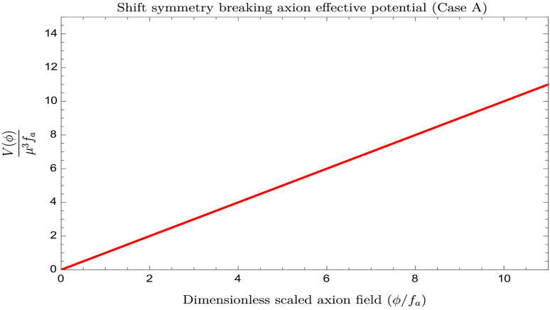
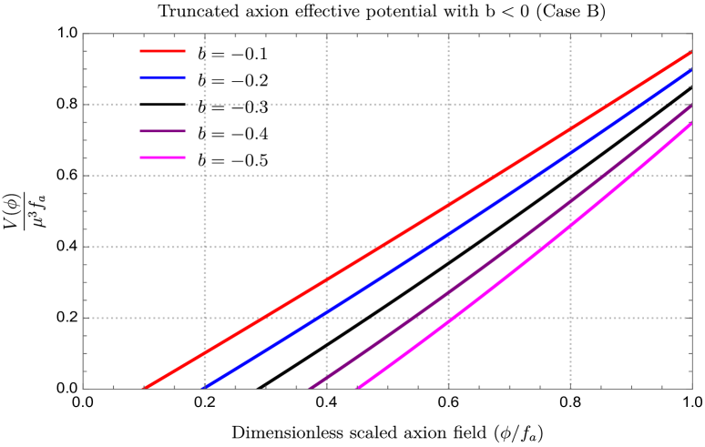
Refer to caption
Figure 3.5: Schematic behaviour of the approximated axion effective potential obtained from Case A.
𝐒𝐭𝐫𝐢𝐧𝐠𝐬𝐜𝐚𝐥𝐞:Ms=1αexp(A0)=(ΛGmSUSY)2LRgs=L4mSUSYRgsexp(cSinst)𝐈𝐧𝐬𝐭𝐚𝐧𝐭𝐨𝐧𝐢𝐜𝐝𝐞𝐜𝐚𝐲\displaystyle{\bf String\leavevmode\nobreak\ scale:}\leavevmode\nobreak\ \leavevmode\nobreak\ \leavevmode\nobreak\ \leavevmode\nobreak\ \leavevmode\nobreak\ M_{s}=\frac{1}{\sqrt{\alpha^{{}^{\prime}}}}\exp(A_{0})=\left(\frac{\Lambda_{G}}{m_{SUSY}}\right)^{2}\frac{L}{R}\sqrt{g_{s}}=\frac{L^{4}}{m_{SUSY}R\sqrt{g_{s}}}\leavevmode\nobreak\ \underbrace{\exp\left(-cS_{inst}\right)}_{\bf Instantonic\leavevmode\nobreak\ decay}
Refer to caption
(a) For b<0𝑏0b<0
Refer to caption
(b) For b>0𝑏0b>0
Figure 3.6: Schematic behaviour of the truncated axion effective potential obtained from Case B with stringy parameter b<0𝑏0b<0 and b>0𝑏0b>0.

The representative action along with the effective potential is a very important input for the rest of the computation performed in this paper.

Here the following two physical approximation can be used to simplify the problem in a very simpler language:

  1. 1.

    Case A:
    This is the specific situation where we only consider the part of the effective potential which breaks the shift symmetry ϕϕ+2πfaitalic-ϕitalic-ϕ2𝜋subscript𝑓𝑎\phi\rightarrow\phi+2\pi f_{a}, which is given by:

    𝐒𝐡𝐢𝐟𝐭𝐬𝐲𝐦𝐦𝐞𝐭𝐫𝐲𝐛𝐫𝐞𝐚𝐤𝐢𝐧𝐠𝐞𝐟𝐟𝐞𝐜𝐭𝐢𝐯𝐞𝐩𝐨𝐭𝐞𝐧𝐭𝐢𝐚𝐥:V(ϕ)μ3fa(ϕfa).\displaystyle{\bf Shift\leavevmode\nobreak\ symmetry\leavevmode\nobreak\ breaking\leavevmode\nobreak\ effective\leavevmode\nobreak\ potential:}\leavevmode\nobreak\ \leavevmode\nobreak\ V(\phi)\approx\mu^{3}f_{a}\left(\frac{\phi}{f_{a}}\right). (3.45)

    In the present computational purpose, particularly in the field equation the above mentioned potential contributes as a source term in terms of μ3superscript𝜇3\mu^{3} which basically fix the overall energy scale in terms of the stringy model parameters. In figure (3.5), the corresponding shift symmetry breaking part of the axion effective potential is plotted, which shows linear behaviour.

  2. 2.

    Case B:
    In this specific case we consider the small field limiting approximation in which the dimensionless field variable ϕfa1much-less-thanitalic-ϕsubscript𝑓𝑎1\displaystyle\frac{\phi}{f_{a}}\ll 1. For this reason one can approximate the shift symmetry ϕϕ+2πfaitalic-ϕitalic-ϕ2𝜋subscript𝑓𝑎\phi\rightarrow\phi+2\pi f_{a} preserving non-perturbative contribution as:

    cos(ϕfa)112(ϕfa)2,italic-ϕsubscript𝑓𝑎112superscriptitalic-ϕsubscript𝑓𝑎2\displaystyle\displaystyle\cos\left(\frac{\phi}{f_{a}}\right)\approx 1-\frac{1}{2}\left(\frac{\phi}{f_{a}}\right)^{2}, (3.46)

    where due to having the truncation at the quadratic order term at the end t.he previously mentioned shift symmetry is broken. In prince one can take the full non-perturbative term, but at the level of eqn of motion and later deling with such terms are extremely difficult in the field theory language. In the present computational purpose the higher order terms can be neglected due to having small field limit without loosing any generality, on the cost of breaking the shift symmetry. Consequently in the present case the effective potential can be approximated as:

    𝐓𝐫𝐮𝐧𝐜𝐚𝐭𝐞𝐝𝐞𝐟𝐟𝐞𝐜𝐭𝐢𝐯𝐞𝐩𝐨𝐭𝐞𝐧𝐭𝐢𝐚𝐥:V(ϕ)\displaystyle{\bf Truncated\leavevmode\nobreak\ effective\leavevmode\nobreak\ potential:}\leavevmode\nobreak\ \leavevmode\nobreak\ \leavevmode\nobreak\ \leavevmode\nobreak\ \leavevmode\nobreak\ V(\phi) \displaystyle\approx ΛG4+μ3fa(ϕfa)ΛG42(ϕfa)2subscriptsuperscriptΛ4𝐺superscript𝜇3subscript𝑓𝑎italic-ϕsubscript𝑓𝑎subscriptsuperscriptΛ4𝐺2superscriptitalic-ϕsubscript𝑓𝑎2\displaystyle\Lambda^{4}_{G}+\mu^{3}f_{a}\left(\frac{\phi}{f_{a}}\right)-\frac{\Lambda^{4}_{G}}{2}\left(\frac{\phi}{f_{a}}\right)^{2} (3.47)
    =\displaystyle= μ3fa(b+(ϕfa))meff22(ϕfa)2superscript𝜇3subscript𝑓𝑎𝑏italic-ϕsubscript𝑓𝑎subscriptsuperscript𝑚2𝑒𝑓𝑓2superscriptitalic-ϕsubscript𝑓𝑎2\displaystyle\mu^{3}f_{a}\left(b+\left(\frac{\phi}{f_{a}}\right)\right)-\frac{m^{2}_{eff}}{2}\left(\frac{\phi}{f_{a}}\right)^{2}
    =\displaystyle= μ3fa(b+(ϕfa)b2(ϕfa)2),superscript𝜇3subscript𝑓𝑎𝑏italic-ϕsubscript𝑓𝑎𝑏2superscriptitalic-ϕsubscript𝑓𝑎2\displaystyle\mu^{3}f_{a}\left(b+\left(\frac{\phi}{f_{a}}\right)-\frac{b}{2}\left(\frac{\phi}{f_{a}}\right)^{2}\right),\leavevmode\nobreak\ \leavevmode\nobreak\ \leavevmode\nobreak\ \leavevmode\nobreak\ \leavevmode\nobreak\ \leavevmode\nobreak\ \leavevmode\nobreak\ \leavevmode\nobreak\ \leavevmode\nobreak\ \leavevmode\nobreak\

    where we define the effective mass in terms of stringy parameters by the following expression:

    𝐄𝐟𝐟𝐞𝐜𝐭𝐢𝐯𝐞𝐦𝐚𝐬𝐬:meff2\displaystyle{\bf Effective\leavevmode\nobreak\ mass:}\leavevmode\nobreak\ \leavevmode\nobreak\ \leavevmode\nobreak\ \leavevmode\nobreak\ \leavevmode\nobreak\ m^{2}_{eff} =\displaystyle= μ3bfa=ΛG4=(mSUSYL3αgs)2exp(4cSinst)𝐈𝐧𝐬𝐭𝐚𝐧𝐭𝐨𝐧𝐢𝐜𝐝𝐞𝐜𝐚𝐲.superscript𝜇3𝑏subscript𝑓𝑎subscriptsuperscriptΛ4𝐺superscriptsubscript𝑚𝑆𝑈𝑆𝑌superscript𝐿3superscript𝛼subscript𝑔𝑠2subscript4𝑐subscript𝑆𝑖𝑛𝑠𝑡𝐈𝐧𝐬𝐭𝐚𝐧𝐭𝐨𝐧𝐢𝐜𝐝𝐞𝐜𝐚𝐲\displaystyle\mu^{3}bf_{a}=\Lambda^{4}_{G}=\left(\frac{m_{SUSY}L^{3}}{\sqrt{\alpha^{{}^{\prime}}}g_{s}}\right)^{2}\leavevmode\nobreak\ \underbrace{\exp\left(-4cS_{inst}\right)}_{\bf Instantonic\leavevmode\nobreak\ decay}.\leavevmode\nobreak\ \leavevmode\nobreak\ \leavevmode\nobreak\ \leavevmode\nobreak\ \leavevmode\nobreak\ \leavevmode\nobreak\ \leavevmode\nobreak\ \leavevmode\nobreak\ \leavevmode\nobreak\ \leavevmode\nobreak\ (3.48)

    In figure (3.6(a)) and figure (3.6(b)), the corresponding trucated axion effective potential is plotted, which shows deviation from the linear behaviour for both the signatures of stringy parameter b<0𝑏0b<0 and b>0𝑏0b>0 for small field limit where ϕfamuch-less-thanitalic-ϕsubscript𝑓𝑎\phi\ll f_{a} approximation works perfectly well.

We are now interested in the field equations of axion which can be obtained by varying the effective action stated in equation (3.33) with respect to the axion field itself, give rise to the following expressions for the above mentioned two cases:

𝐅𝐨𝐫𝐂𝐚𝐬𝐞𝐀:¯[1a3(t)t(a3(t)t)1H2a2(t)𝐋^𝐇𝟑2]ϕ¯:𝐅𝐨𝐫𝐂𝐚𝐬𝐞𝐀absentdelimited-[]1superscript𝑎3𝑡subscript𝑡superscript𝑎3𝑡subscript𝑡1superscript𝐻2superscript𝑎2𝑡subscriptsuperscript^𝐋2superscript𝐇3italic-ϕ\displaystyle\underline{{\color[rgb]{0,0,0}\definecolor[named]{pgfstrokecolor}{rgb}{0,0,0}\pgfsys@color@gray@stroke{0}\pgfsys@color@gray@fill{0}\bf For\leavevmode\nobreak\ Case\leavevmode\nobreak\ A}:}\leavevmode\nobreak\ \leavevmode\nobreak\ \leavevmode\nobreak\ \leavevmode\nobreak\ \leavevmode\nobreak\ \leavevmode\nobreak\ \leavevmode\nobreak\ \leavevmode\nobreak\ \leavevmode\nobreak\ \leavevmode\nobreak\ \leavevmode\nobreak\ \leavevmode\nobreak\ \leavevmode\nobreak\ \leavevmode\nobreak\ \leavevmode\nobreak\ \leavevmode\nobreak\ \leavevmode\nobreak\ \leavevmode\nobreak\ \leavevmode\nobreak\ \leavevmode\nobreak\ \leavevmode\nobreak\ \leavevmode\nobreak\ \leavevmode\nobreak\ \leavevmode\nobreak\ \leavevmode\nobreak\ \leavevmode\nobreak\ \leavevmode\nobreak\ \leavevmode\nobreak\ \leavevmode\nobreak\ \leavevmode\nobreak\ \left[\frac{1}{a^{3}(t)}\partial_{t}\left(a^{3}(t)\partial_{t}\right)-\frac{1}{H^{2}a^{2}(t)}\hat{\bf L}^{2}_{\bf H^{3}}\right]\phi =\displaystyle= μ3,superscript𝜇3\displaystyle\mu^{3}, (3.49)
𝐅𝐨𝐫𝐂𝐚𝐬𝐞𝐁:¯([1a3(t)t(a3(t)t)1H2a2(t)𝐋^𝐇𝟑2]+meff2)ϕ¯:𝐅𝐨𝐫𝐂𝐚𝐬𝐞𝐁absentdelimited-[]1superscript𝑎3𝑡subscript𝑡superscript𝑎3𝑡subscript𝑡1superscript𝐻2superscript𝑎2𝑡subscriptsuperscript^𝐋2superscript𝐇3subscriptsuperscript𝑚2𝑒𝑓𝑓italic-ϕ\displaystyle\underline{{\color[rgb]{0,0,0}\definecolor[named]{pgfstrokecolor}{rgb}{0,0,0}\pgfsys@color@gray@stroke{0}\pgfsys@color@gray@fill{0}\bf For\leavevmode\nobreak\ Case\leavevmode\nobreak\ B}:}\leavevmode\nobreak\ \leavevmode\nobreak\ \leavevmode\nobreak\ \leavevmode\nobreak\ \leavevmode\nobreak\ \leavevmode\nobreak\ \leavevmode\nobreak\ \leavevmode\nobreak\ \leavevmode\nobreak\ \leavevmode\nobreak\ \leavevmode\nobreak\ \leavevmode\nobreak\ \leavevmode\nobreak\ \leavevmode\nobreak\ \leavevmode\nobreak\ \left(\left[\frac{1}{a^{3}(t)}\partial_{t}\left(a^{3}(t)\partial_{t}\right)-\frac{1}{H^{2}a^{2}(t)}\hat{\bf L}^{2}_{\bf H^{3}}\right]+m^{2}_{eff}\right)\phi =\displaystyle= μ3=meff2fab,superscript𝜇3subscriptsuperscript𝑚2𝑒𝑓𝑓subscript𝑓𝑎𝑏\displaystyle\mu^{3}=\frac{m^{2}_{eff}f_{a}}{b},

where the scale factor a(t)𝑎𝑡a(t) for global de Sitter space is given by the following expression:

𝐒𝐜𝐚𝐥𝐞𝐟𝐚𝐜𝐭𝐨𝐫a(t)𝐒𝐜𝐚𝐥𝐞𝐟𝐚𝐜𝐭𝐨𝐫𝑎𝑡\displaystyle\displaystyle{\color[rgb]{0,0,0}\definecolor[named]{pgfstrokecolor}{rgb}{0,0,0}\pgfsys@color@gray@stroke{0}\pgfsys@color@gray@fill{0}\bf Scale\leavevmode\nobreak\ factor}\leavevmode\nobreak\ \leavevmode\nobreak\ \leavevmode\nobreak\ \leavevmode\nobreak\ \leavevmode\nobreak\ \leavevmode\nobreak\ \leavevmode\nobreak\ \leavevmode\nobreak\ \leavevmode\nobreak\ \leavevmode\nobreak\ \leavevmode\nobreak\ \leavevmode\nobreak\ \leavevmode\nobreak\ \leavevmode\nobreak\ a(t) =\displaystyle= 1Hsinhtwheret=(t𝐑(in𝐑),t𝐋(in𝐋)).1𝐻𝑡where𝑡subscript𝑡𝐑in𝐑subscript𝑡𝐋in𝐋\displaystyle\displaystyle\frac{1}{H}\sinh t\leavevmode\nobreak\ \leavevmode\nobreak\ \leavevmode\nobreak\ \leavevmode\nobreak\ {\rm where}\leavevmode\nobreak\ \leavevmode\nobreak\ \leavevmode\nobreak\ t=\Bigg{(}t_{\bf R}({\rm in}\leavevmode\nobreak\ {\bf R}),t_{\bf L}({\rm in}\leavevmode\nobreak\ {\bf L})\Bigg{)}. (3.51)

In this context we introduce a Laplacian operator 𝐋^𝐇𝟑2subscriptsuperscript^𝐋2superscript𝐇3\hat{\bf L}^{2}_{\bf H^{3}} in hyperbolic slice 𝐇𝟑superscript𝐇3{\bf H^{3}} which is defined as:

𝐋𝐚𝐩𝐥𝐚𝐜𝐢𝐚𝐧𝐨𝐩𝐞𝐫𝐚𝐭𝐨𝐫:𝐋^𝐇𝟑2\displaystyle{\color[rgb]{0,0,0}\definecolor[named]{pgfstrokecolor}{rgb}{0,0,0}\pgfsys@color@gray@stroke{0}\pgfsys@color@gray@fill{0}\bf Laplacian\leavevmode\nobreak\ operator:}\leavevmode\nobreak\ \leavevmode\nobreak\ \leavevmode\nobreak\ \leavevmode\nobreak\ \hat{\bf L}^{2}_{\bf H^{3}} =\displaystyle= 1sinh2r[r(sinh2rr)+1sinθθ(sinθθ)+1sin2θΦ2].1superscript2𝑟delimited-[]subscript𝑟superscript2𝑟subscript𝑟1𝜃subscript𝜃𝜃subscript𝜃1superscript2𝜃subscriptsuperscript2Φ\displaystyle\frac{1}{\sinh^{2}r}\left[\partial_{r}\left(\sinh^{2}r\leavevmode\nobreak\ \partial_{r}\right)+\frac{1}{\sin\theta}\partial_{\theta}\left(\sin\theta\leavevmode\nobreak\ \partial_{\theta}\right)+\frac{1}{\sin^{2}\theta}\partial^{2}_{\Phi}\right].

which has the following properties:

  1. 1.

    Laplacian operator 𝐋^𝐇𝟑2subscriptsuperscript^𝐋2superscript𝐇3\hat{\bf L}^{2}_{\bf H^{3}} satisfies the following eigenvalue equation:

    𝐄𝐢𝐠𝐞𝐧𝐯𝐚𝐥𝐮𝐞𝐞𝐪𝐮𝐚𝐭𝐢𝐨𝐧:𝐋^𝐇𝟑2𝒴plm(r,θ,Φ)\displaystyle{\color[rgb]{0,0,0}\definecolor[named]{pgfstrokecolor}{rgb}{0,0,0}\pgfsys@color@gray@stroke{0}\pgfsys@color@gray@fill{0}\bf Eigenvalue\leavevmode\nobreak\ equation:}\leavevmode\nobreak\ \leavevmode\nobreak\ \leavevmode\nobreak\ \leavevmode\nobreak\ \hat{\bf L}^{2}_{\bf H^{3}}{\rm\cal Y}_{plm}(r,\theta,\Phi) =\displaystyle= λp𝒴plm(r,θ,Φ),subscript𝜆𝑝subscript𝒴𝑝𝑙𝑚𝑟𝜃Φ\displaystyle\lambda_{p}{\rm\cal Y}_{plm}(r,\theta,\Phi), (3.53)

    with quantum number p𝑝p dependent eigenvalue:

    𝐄𝐢𝐠𝐞𝐧𝐯𝐚𝐥𝐮𝐞:λp=(1+p2).\displaystyle{\color[rgb]{0,0,0}\definecolor[named]{pgfstrokecolor}{rgb}{0,0,0}\pgfsys@color@gray@stroke{0}\pgfsys@color@gray@fill{0}\bf Eigenvalue:}\leavevmode\nobreak\ \leavevmode\nobreak\ \leavevmode\nobreak\ \leavevmode\nobreak\ \lambda_{p}=-(1+p^{2}). (3.54)
  2. 2.

    Eigenfunction of the Laplacian operator 𝐋^𝐇𝟑2subscriptsuperscript^𝐋2superscript𝐇3\hat{\bf L}^{2}_{\bf H^{3}} is 𝒴plm(r,θ,Φ)subscript𝒴𝑝𝑙𝑚𝑟𝜃Φ{\rm\cal Y}_{plm}(r,\theta,\Phi) which is defined as:

    𝐄𝐢𝐠𝐞𝐧𝐟𝐮𝐧𝐜𝐭𝐢𝐨𝐧:𝒴plm(r,θ,Φ)\displaystyle{\color[rgb]{0,0,0}\definecolor[named]{pgfstrokecolor}{rgb}{0,0,0}\pgfsys@color@gray@stroke{0}\pgfsys@color@gray@fill{0}\bf Eigenfunction:}\leavevmode\nobreak\ \leavevmode\nobreak\ \leavevmode\nobreak\ \leavevmode\nobreak\ {\cal Y}_{plm}(r,\theta,\Phi) =\displaystyle= Γ(ip+l+1)Γ(ip+1)psinhr𝒫(ip12)(l+12)(coshr)Ylm(θ,Φ),Γ𝑖𝑝𝑙1Γ𝑖𝑝1𝑝𝑟subscriptsuperscript𝒫𝑙12𝑖𝑝12𝑟subscript𝑌𝑙𝑚𝜃Φ\displaystyle\frac{\Gamma\left(ip+l+1\right)}{\Gamma\left(ip+1\right)}\leavevmode\nobreak\ \frac{p}{\sqrt{\sinh r}}\leavevmode\nobreak\ {\cal P}^{-\left(l+\frac{1}{2}\right)}_{\left(ip-\frac{1}{2}\right)}\left(\cosh r\right)Y_{lm}(\theta,\Phi),

    where p𝑝p, l𝑙l and m𝑚m are three quantum numbers associated with the above mentioned eigenfunction. Here Ylm(θ,Φ)subscript𝑌𝑙𝑚𝜃ΦY_{lm}(\theta,\Phi) is the well known spherical harmonics which is dependent on two quantum numbers l𝑙l and m𝑚m and on two angular coordinates as it defined in 𝐒2superscript𝐒2{\bf S}^{2} and last but not the least the radial solution is characterized by the function, 𝒫(ip12)(l+12)(coshr)subscriptsuperscript𝒫𝑙12𝑖𝑝12𝑟{\cal P}^{-\left(l+\frac{1}{2}\right)}_{\left(ip-\frac{1}{2}\right)}\left(\cosh r\right), which is the well known associated Legendre polynomial in this context.

After quantization the classical solution obtained from the field equation is promoted in terms of the quantum operator and by following the well known canonical quantization technique the corresponding quantum operator can be written in terms of the creation and annihilation operators along with basis Bunch Davies mode function, which is nothing but the classical counterpart of the solution of the field equation. The total quantum solution for the axion field operator for both the Case A and Case B can be written in the following compact form:

𝐐𝐮𝐚𝐧𝐭𝐮𝐦𝐌𝐨𝐝𝐞𝐟𝐮𝐧𝐜𝐭𝐢𝐨𝐧:ϕ^(t,r,θ,Φ)\displaystyle{\color[rgb]{0,0,0}\definecolor[named]{pgfstrokecolor}{rgb}{0,0,0}\pgfsys@color@gray@stroke{0}\pgfsys@color@gray@fill{0}\bf Quantum\leavevmode\nobreak\ Mode\leavevmode\nobreak\ function:}\leavevmode\nobreak\ \leavevmode\nobreak\ \leavevmode\nobreak\ \leavevmode\nobreak\ \widehat{\phi}(t,r,\theta,\Phi) =\displaystyle= 0dpσ=±1l=0p1m=l+l[aσplm𝒰σplm(t,r,θ,Φ)\displaystyle\int^{\infty}_{0}dp\sum_{\sigma=\pm 1}\sum^{p-1}_{l=0}\sum^{+l}_{m=-l}\left[a_{\sigma plm}{\cal U}_{\sigma plm}(t,r,\theta,\Phi)\right.
+aσplm𝒰σplm(t,r,θ,Φ)]t=(t𝐑,t𝐋).\displaystyle\left.\leavevmode\nobreak\ \leavevmode\nobreak\ \leavevmode\nobreak\ \leavevmode\nobreak\ \leavevmode\nobreak\ +a^{\dagger}_{\sigma plm}{\cal U}^{*}_{\sigma plm}(t,r,\theta,\Phi)\right]\forall\leavevmode\nobreak\ \leavevmode\nobreak\ t=(t_{\bf R},t_{\bf L}).

In this context the Bunch-Davies vacuum is defined by the following expression:

𝐁𝐮𝐧𝐜𝐡𝐃𝐚𝐯𝐢𝐞𝐬𝐯𝐚𝐜𝐮𝐮𝐦:aσplm|𝐁𝐃\displaystyle{\color[rgb]{0,0,0}\definecolor[named]{pgfstrokecolor}{rgb}{0,0,0}\pgfsys@color@gray@stroke{0}\pgfsys@color@gray@fill{0}\bf Bunch-Davies\leavevmode\nobreak\ vacuum:}\leavevmode\nobreak\ \leavevmode\nobreak\ a_{\sigma plm}|{\bf BD}\rangle =\displaystyle= 0σ=(+1,1);0<p<;formulae-sequence0for-all𝜎110𝑝\displaystyle 0\leavevmode\nobreak\ \leavevmode\nobreak\ \leavevmode\nobreak\ \leavevmode\nobreak\ \leavevmode\nobreak\ \leavevmode\nobreak\ \leavevmode\nobreak\ \leavevmode\nobreak\ \leavevmode\nobreak\ \leavevmode\nobreak\ \forall\sigma=(+1,-1);0<p<\infty; (3.57)
l=0,,p1,m=l,,+l.formulae-sequence𝑙0𝑝1𝑚𝑙𝑙\displaystyle\leavevmode\nobreak\ \leavevmode\nobreak\ \leavevmode\nobreak\ \leavevmode\nobreak\ \leavevmode\nobreak\ \leavevmode\nobreak\ \leavevmode\nobreak\ \leavevmode\nobreak\ \leavevmode\nobreak\ \leavevmode\nobreak\ \leavevmode\nobreak\ \leavevmode\nobreak\ l=0,\cdots,p-1,m=-l,\cdots,+l.\leavevmode\nobreak\ \leavevmode\nobreak\ \leavevmode\nobreak\ \leavevmode\nobreak\ \leavevmode\nobreak\ \leavevmode\nobreak\ \leavevmode\nobreak\ \leavevmode\nobreak\ \leavevmode\nobreak\ \leavevmode\nobreak\ \leavevmode\nobreak\

Here 𝒰σplm(t,r,θ,Φ)subscript𝒰𝜎𝑝𝑙𝑚𝑡𝑟𝜃Φ{\cal U}_{\sigma plm}(t,r,\theta,\Phi) represents the classical solution of the field equation for the axion for both the Case A and Case B which forms the complete basis. After quantization this basis functions, which is sometimes referred as the mode functions are tagged by the three quantum numbers, p𝑝p, l𝑙l and m𝑚m, which are appearing as an outcome of the canonical quantization of the modes in the present context of discussion. The solution of the mode functions can be obtained by solving the corresponding axion field equations, which are basically solving partial differential equations using the well known method of separation of variables for the Case A and Case B. This finally give rise to the following expression for both the mentioned possibilities:

𝐁𝐮𝐧𝐜𝐡𝐃𝐚𝐯𝐢𝐞𝐬𝐌𝐨𝐝𝐞𝐟𝐮𝐧𝐜𝐭𝐢𝐨𝐧:𝒰σplm(t,r,θ,Φ)\displaystyle{\color[rgb]{0,0,0}\definecolor[named]{pgfstrokecolor}{rgb}{0,0,0}\pgfsys@color@gray@stroke{0}\pgfsys@color@gray@fill{0}\bf Bunch-Davies\leavevmode\nobreak\ Mode\leavevmode\nobreak\ function:}\leavevmode\nobreak\ \leavevmode\nobreak\ {\cal U}_{\sigma plm}(t,r,\theta,\Phi) =\displaystyle= 1a(t)χp,σ(t)𝒴plm(r,θ,Φ)1𝑎𝑡subscript𝜒𝑝𝜎𝑡subscript𝒴𝑝𝑙𝑚𝑟𝜃Φ\displaystyle\frac{1}{a(t)}\chi_{p,\sigma}(t){\cal Y}_{plm}(r,\theta,\Phi) (3.58)
=\displaystyle= Hsinhtχp,σ(t)𝒴plm(r,θ,Φ).𝐻𝑡subscript𝜒𝑝𝜎𝑡subscript𝒴𝑝𝑙𝑚𝑟𝜃Φ\displaystyle\frac{H}{\sinh t}\chi_{p,\sigma}(t){\cal Y}_{plm}(r,\theta,\Phi).\leavevmode\nobreak\ \leavevmode\nobreak\ \leavevmode\nobreak\ \leavevmode\nobreak\ \leavevmode\nobreak\ \leavevmode\nobreak\ \leavevmode\nobreak\ \leavevmode\nobreak\

Here it is important to note that the time dependent part of the mode function χp,σ(t)subscript𝜒𝑝𝜎𝑡\chi_{p,\sigma}(t) only works for the positive frequencies and hence forms a complete set in the present theoretical set up. This part of the solution is dependent on the momentum p𝑝p which is actually the wave number and in the quantum mechanical picture it is playing the role of a quantum number as clearly mentioned earlier. Particularly this time dependent part of the wave function is extremely significant for the present discussion as we are interested in the dynamical behaviour of the mode function in the R and L region of the open chart of global de Sitter space time. This particular part will going to control the behaviour of the quantum entanglement measure in the mentioned space time. If we can able to extract the hidden features from the time dependent part of the field equations from the Case A and Case B then half of the computational job is done. Now since in both the cases we are dealing with inhomogeneous second order differential equations the total solution can be written as the sum of complementary part (χp,σ(c)(t)subscriptsuperscript𝜒𝑐𝑝𝜎𝑡\chi^{(c)}_{p,\sigma}(t)) and particular integral part (χp,σ(p)(t)subscriptsuperscript𝜒𝑝𝑝𝜎𝑡\chi^{(p)}_{p,\sigma}(t)) i.e.

𝐓𝐨𝐭𝐚𝐥𝐭𝐢𝐦𝐞𝐝𝐞𝐩𝐞𝐧𝐝𝐞𝐧𝐭𝐬𝐨𝐥𝐮𝐭𝐢𝐨𝐧:χp,σ(t)=χp,σ(C)(t)𝐂𝐨𝐦𝐩𝐥𝐞𝐦𝐞𝐧𝐭𝐚𝐫𝐲𝐩𝐚𝐫𝐭+χp,σ(P)(t)𝐏𝐚𝐫𝐭𝐢𝐜𝐮𝐥𝐚𝐫𝐢𝐧𝐭𝐞𝐠𝐫𝐚𝐥𝐩𝐚𝐫𝐭.\displaystyle{\color[rgb]{0,0,0}\definecolor[named]{pgfstrokecolor}{rgb}{0,0,0}\pgfsys@color@gray@stroke{0}\pgfsys@color@gray@fill{0}\bf Total\leavevmode\nobreak\ time\leavevmode\nobreak\ dependent\leavevmode\nobreak\ solution:}\leavevmode\nobreak\ \leavevmode\nobreak\ \chi_{p,\sigma}(t)=\underbrace{\chi^{(C)}_{p,\sigma}(t)}_{\bf Complementary\leavevmode\nobreak\ part}+\underbrace{\chi^{(P)}_{p,\sigma}(t)}_{\bf Particular\leavevmode\nobreak\ integral\leavevmode\nobreak\ part}.

Here the complementary part (χp,σ(c)(t)subscriptsuperscript𝜒𝑐𝑝𝜎𝑡\chi^{(c)}_{p,\sigma}(t)) of the time dependent solution of the mode function satisfy the homogeneous part of the field equation for the Case A and Case B can be written as:

𝐂𝐨𝐦𝐩𝐥𝐞𝐦𝐞𝐧𝐭𝐚𝐫𝐲𝐩𝐚𝐫𝐭𝐨𝐟𝐭𝐡𝐞𝐟𝐢𝐞𝐥𝐝𝐞𝐪𝐮𝐚𝐭𝐢𝐨𝐧::𝐂𝐨𝐦𝐩𝐥𝐞𝐦𝐞𝐧𝐭𝐚𝐫𝐲𝐩𝐚𝐫𝐭𝐨𝐟𝐭𝐡𝐞𝐟𝐢𝐞𝐥𝐝𝐞𝐪𝐮𝐚𝐭𝐢𝐨𝐧absent\displaystyle{\color[rgb]{0,0,0}\definecolor[named]{pgfstrokecolor}{rgb}{0,0,0}\pgfsys@color@gray@stroke{0}\pgfsys@color@gray@fill{0}\bf Complementary\leavevmode\nobreak\ part\leavevmode\nobreak\ of\leavevmode\nobreak\ the\leavevmode\nobreak\ field\leavevmode\nobreak\ equation:}\leavevmode\nobreak\ \leavevmode\nobreak\
00\displaystyle\displaystyle 0 =\displaystyle= {[t2+3cothtt+(1+p2)sinh2t]χp,σ(C)(t)for Case A[t2+3cothtt+(1+p2)sinh2t+meff2H2]χp,σ(C)(t)for Case B.casesdelimited-[]subscriptsuperscript2𝑡3hyperbolic-cotangent𝑡subscript𝑡1superscript𝑝2superscript2𝑡subscriptsuperscript𝜒𝐶𝑝𝜎𝑡for Case Amissing-subexpressionmissing-subexpressiondelimited-[]subscriptsuperscript2𝑡3hyperbolic-cotangent𝑡subscript𝑡1superscript𝑝2superscript2𝑡subscriptsuperscript𝑚2𝑒𝑓𝑓superscript𝐻2subscriptsuperscript𝜒𝐶𝑝𝜎𝑡for Case B\displaystyle\displaystyle\left\{\begin{array}[]{ll}\displaystyle\left[\partial^{2}_{t}+3\coth t\leavevmode\nobreak\ \partial_{t}+\frac{(1+p^{2})}{\sinh^{2}t}\right]\chi^{(C)}_{p,\sigma}(t)\nobreak\leavevmode\nobreak\leavevmode\nobreak\leavevmode\nobreak\leavevmode\nobreak\leavevmode\nobreak\leavevmode\nobreak\leavevmode\nobreak\leavevmode\nobreak\leavevmode\nobreak\leavevmode\nobreak\leavevmode\nobreak\leavevmode\nobreak\leavevmode\nobreak\leavevmode\nobreak\leavevmode\nobreak\leavevmode\nobreak\leavevmode&\mbox{\small{{\color[rgb]{0,0,0}\definecolor[named]{pgfstrokecolor}{rgb}{0,0,0}\pgfsys@color@gray@stroke{0}\pgfsys@color@gray@fill{0}\bf for Case A}}}\\ \\ \displaystyle\left[\partial^{2}_{t}+3\coth t\leavevmode\nobreak\ \partial_{t}+\frac{(1+p^{2})}{\sinh^{2}t}+\frac{m^{2}_{eff}}{H^{2}}\right]\chi^{(C)}_{p,\sigma}(t)&\mbox{\small{{\color[rgb]{0,0,0}\definecolor[named]{pgfstrokecolor}{rgb}{0,0,0}\pgfsys@color@gray@stroke{0}\pgfsys@color@gray@fill{0}\bf for Case B}}}.\nobreak\leavevmode\nobreak\leavevmode\nobreak\leavevmode\nobreak\leavevmode\nobreak\leavevmode\nobreak\leavevmode\nobreak\leavevmode\nobreak\leavevmode\end{array}\right. (3.63)

The solution of the above equations for the Case A and Case B combiningly can be written as:

𝐂𝐨𝐦𝐩𝐥𝐞𝐦𝐞𝐧𝐭𝐚𝐫𝐲𝐬𝐨𝐥𝐮𝐭𝐢𝐨𝐧::𝐂𝐨𝐦𝐩𝐥𝐞𝐦𝐞𝐧𝐭𝐚𝐫𝐲𝐬𝐨𝐥𝐮𝐭𝐢𝐨𝐧absent\displaystyle{\color[rgb]{0,0,0}\definecolor[named]{pgfstrokecolor}{rgb}{0,0,0}\pgfsys@color@gray@stroke{0}\pgfsys@color@gray@fill{0}\bf Complementary\leavevmode\nobreak\ solution:}\leavevmode\nobreak\ \leavevmode\nobreak\
χp,σ(c)(t)subscriptsuperscript𝜒𝑐𝑝𝜎𝑡\displaystyle\chi^{(c)}_{p,\sigma}(t) =\displaystyle= {{12sinhπp[(eπpiσeiπν)Γ(ν+12+ip)𝒫(ν12)ip(cosht𝐑)(eπpiσeiπν)Γ(ν+12ip)𝒫(ν12)ip(cosht𝐑)]}σ=±1for R{σ2sinhπp[(eπpiσeiπν)Γ(ν+12+ip)𝒫(ν12)ip(cosht𝐋)(eπpiσeiπν)Γ(ν+12ip)𝒫(ν12)ip(cosht𝐋)]}σ=±1for L,\displaystyle\displaystyle\left\{\begin{array}[]{ll}\displaystyle\left\{\frac{1}{2\sinh\pi p}\left[\frac{\left(e^{\pi p}-i\sigma\leavevmode\nobreak\ e^{-i\pi\nu}\right)}{\Gamma\left(\nu+\frac{1}{2}+ip\right)}{\cal P}^{ip}_{\left(\nu-\frac{1}{2}\right)}(\cosh t_{\bf R})\displaystyle\right.\right.\\ \left.\left.\displaystyle\leavevmode\nobreak\ \leavevmode\nobreak\ \leavevmode\nobreak\ \leavevmode\nobreak\ \leavevmode\nobreak\ \leavevmode\nobreak\ \leavevmode\nobreak\ \leavevmode\nobreak\ \leavevmode\nobreak\ \leavevmode\nobreak\ \leavevmode\nobreak\ \leavevmode\nobreak\ \leavevmode\nobreak\ \leavevmode\nobreak\ -\frac{\left(e^{-\pi p}-i\sigma\leavevmode\nobreak\ e^{-i\pi\nu}\right)}{\Gamma\left(\nu+\frac{1}{2}-ip\right)}{\cal P}^{-ip}_{\left(\nu-\frac{1}{2}\right)}(\cosh t_{\bf R})\right]\right\}_{\sigma=\pm 1}\nobreak\leavevmode\nobreak\leavevmode&\leavevmode\nobreak\ \leavevmode\nobreak\ \leavevmode\nobreak\ \leavevmode\nobreak\ \leavevmode\nobreak\ \leavevmode\nobreak\ \leavevmode\nobreak\ \leavevmode\nobreak\ \leavevmode\nobreak\ \leavevmode\nobreak\ \leavevmode\nobreak\ \leavevmode\nobreak\ \leavevmode\nobreak\ \leavevmode\nobreak\ \leavevmode\nobreak\ \leavevmode\nobreak\ \leavevmode\nobreak\ \leavevmode\nobreak\ \leavevmode\nobreak\ \leavevmode\nobreak\ \leavevmode\nobreak\ \leavevmode\nobreak\ \leavevmode\nobreak\ \leavevmode\nobreak\ \mbox{\small{{\color[rgb]{0,0,0}\definecolor[named]{pgfstrokecolor}{rgb}{0,0,0}\pgfsys@color@gray@stroke{0}\pgfsys@color@gray@fill{0}\bf for R}}}\\ \displaystyle\left\{\frac{\sigma}{2\sinh\pi p}\left[\frac{\left(e^{\pi p}-i\sigma\leavevmode\nobreak\ e^{-i\pi\nu}\right)}{\Gamma\left(\nu+\frac{1}{2}+ip\right)}{\cal P}^{ip}_{\left(\nu-\frac{1}{2}\right)}(\cosh t_{\bf L})\displaystyle\displaystyle\right.\right.\\ \left.\left.\displaystyle\leavevmode\nobreak\ \leavevmode\nobreak\ \leavevmode\nobreak\ \leavevmode\nobreak\ \leavevmode\nobreak\ \leavevmode\nobreak\ \leavevmode\nobreak\ \leavevmode\nobreak\ \leavevmode\nobreak\ \leavevmode\nobreak\ \leavevmode\nobreak\ \leavevmode\nobreak\ \leavevmode\nobreak\ \leavevmode\nobreak\ -\frac{\left(e^{-\pi p}-i\sigma\leavevmode\nobreak\ e^{-i\pi\nu}\right)}{\Gamma\left(\nu+\frac{1}{2}-ip\right)}{\cal P}^{-ip}_{\left(\nu-\frac{1}{2}\right)}(\cosh t_{\bf L})\right]\right\}_{\sigma=\pm 1}&\leavevmode\nobreak\ \leavevmode\nobreak\ \leavevmode\nobreak\ \leavevmode\nobreak\ \leavevmode\nobreak\ \leavevmode\nobreak\ \leavevmode\nobreak\ \leavevmode\nobreak\ \leavevmode\nobreak\ \leavevmode\nobreak\ \leavevmode\nobreak\ \leavevmode\nobreak\ \leavevmode\nobreak\ \leavevmode\nobreak\ \leavevmode\nobreak\ \leavevmode\nobreak\ \leavevmode\nobreak\ \leavevmode\nobreak\ \leavevmode\nobreak\ \leavevmode\nobreak\ \leavevmode\nobreak\ \leavevmode\nobreak\ \leavevmode\nobreak\ \leavevmode\nobreak\ \leavevmode\nobreak\ \mbox{\small{{\color[rgb]{0,0,0}\definecolor[named]{pgfstrokecolor}{rgb}{0,0,0}\pgfsys@color@gray@stroke{0}\pgfsys@color@gray@fill{0}\bf for L}}},\nobreak\leavevmode\nobreak\leavevmode\end{array}\right. (3.68)

where we introduce a new parameter ν𝜈\nu, which is known as mass parameter are defined for Case A and Case B as:

𝐌𝐚𝐬𝐬𝐩𝐚𝐫𝐚𝐦𝐞𝐭𝐞𝐫:ν\displaystyle\displaystyle{\color[rgb]{0,0,0}\definecolor[named]{pgfstrokecolor}{rgb}{0,0,0}\pgfsys@color@gray@stroke{0}\pgfsys@color@gray@fill{0}\bf Mass\leavevmode\nobreak\ parameter:}\leavevmode\nobreak\ \leavevmode\nobreak\ \nu =\displaystyle= {32for Case A94meff2H2=94μ3bfaH2=94ΛG4fa2H2for Case B.cases32for Case A94subscriptsuperscript𝑚2𝑒𝑓𝑓superscript𝐻294superscript𝜇3𝑏subscript𝑓𝑎superscript𝐻294subscriptsuperscriptΛ4𝐺subscriptsuperscript𝑓2𝑎superscript𝐻2for Case B\displaystyle\displaystyle\left\{\begin{array}[]{ll}\displaystyle\frac{3}{2}\nobreak\leavevmode\nobreak\leavevmode\nobreak\leavevmode\nobreak\leavevmode\nobreak\leavevmode\nobreak\leavevmode\nobreak\leavevmode\nobreak\leavevmode\nobreak\leavevmode\nobreak\leavevmode\nobreak\leavevmode\nobreak\leavevmode\nobreak\leavevmode\nobreak\leavevmode\nobreak\leavevmode\nobreak\leavevmode\nobreak\leavevmode&\mbox{\small{{\color[rgb]{0,0,0}\definecolor[named]{pgfstrokecolor}{rgb}{0,0,0}\pgfsys@color@gray@stroke{0}\pgfsys@color@gray@fill{0}\bf for Case A}}}\\ \displaystyle\sqrt{\frac{9}{4}-\frac{m^{2}_{eff}}{H^{2}}}=\sqrt{\frac{9}{4}-\frac{\mu^{3}b}{f_{a}H^{2}}}=\sqrt{\frac{9}{4}-\frac{\Lambda^{4}_{G}}{f^{2}_{a}H^{2}}}\nobreak\leavevmode\nobreak\leavevmode\nobreak\leavevmode\nobreak\leavevmode\nobreak\leavevmode\nobreak\leavevmode\nobreak\leavevmode\nobreak\leavevmode\nobreak\leavevmode&\mbox{\small{{\color[rgb]{0,0,0}\definecolor[named]{pgfstrokecolor}{rgb}{0,0,0}\pgfsys@color@gray@stroke{0}\pgfsys@color@gray@fill{0}\bf for Case B}}}.\nobreak\leavevmode\nobreak\leavevmode\nobreak\leavevmode\nobreak\leavevmode\nobreak\leavevmode\nobreak\leavevmode\nobreak\leavevmode\nobreak\leavevmode\end{array}\right. (3.71)

Here the solution has following properties:

  1. 1.

    Here σ=±1𝜎plus-or-minus1\sigma=\pm 1 for R and L regions.

  2. 2.

    In the Case B if we consider meffHmuch-less-thansubscript𝑚𝑒𝑓𝑓𝐻m_{eff}\ll H, the mass parameter is approximated as ν=3/2𝜈32\nu=3/2 which is exactly the Case A.

  3. 3.

    In the Case B if we consider meff=2Hsubscript𝑚𝑒𝑓𝑓2𝐻m_{eff}=\sqrt{2}H, then the mass parameter is given by ν=1/2𝜈12\nu=1/2 and this is the case of conformally coupling.

  4. 4.

    In the Case B if we consider meff<2Hsubscript𝑚𝑒𝑓𝑓2𝐻m_{eff}<\sqrt{2}H, the mass parameter is lying within the range, 1/2<ν<3/212𝜈321/2<\nu<3/2, which is the low mass region.

  5. 5.

    In the Case B if we consider meff=Hsubscript𝑚𝑒𝑓𝑓𝐻m_{eff}=H, then the mass parameter is given by, ν=5/2𝜈52\nu=5/2, which is the intermediate mass region.

  6. 6.

    In the Case B if we consider meffHmuch-greater-thansubscript𝑚𝑒𝑓𝑓𝐻m_{eff}\gg H, then the mass parameter is given by, ν=imeff2H294imeffH𝜈𝑖subscriptsuperscript𝑚2𝑒𝑓𝑓superscript𝐻294𝑖subscript𝑚𝑒𝑓𝑓𝐻\displaystyle\nu=i\sqrt{\frac{m^{2}_{eff}}{H^{2}}-\frac{9}{4}}\approx i\frac{m_{eff}}{H}, which is the high mass region.

  7. 7.

    In the Case B if we consider 2H<meff<3H/22𝐻subscript𝑚𝑒𝑓𝑓3𝐻2\sqrt{2}H<m_{eff}<3H/2, then the mass parameter ν𝜈\nu is lying within the range, 0<ν<1/20𝜈120<\nu<1/2.

  8. 8.

    Complementary part of the solution satisfy, χp,σ(C)(t)=χp,σ(C)(t)subscriptsuperscript𝜒𝐶𝑝𝜎𝑡subscriptsuperscript𝜒𝐶𝑝𝜎𝑡\chi^{(C)}_{p,\sigma}(t)=\chi^{(C)}_{-p,\sigma}(t).

  9. 9.

    Here one can define the following Klien-Gordon inner product in terms of the complementary part of the time dependent fields equation:

    𝐊𝐥𝐢𝐞𝐧𝐆𝐨𝐫𝐝𝐨𝐧𝐩𝐫𝐨𝐝𝐮𝐜𝐭:((χp,σ(C)(t),χp,σ(C)(t)))𝐊𝐆=𝒩pσδσσ,\displaystyle{\bf Klien-Gordon\leavevmode\nobreak\ product:}\leavevmode\nobreak\ \leavevmode\nobreak\ \leavevmode\nobreak\ \leavevmode\nobreak\ \left(\left(\chi^{(C)}_{p,\sigma}(t),\chi^{(C)}_{p,\sigma^{{}^{\prime}}}(t)\right)\right)_{\bf KG}={\cal N}_{p\sigma}\delta_{\sigma\sigma^{{}^{\prime}}}, (3.72)

    where 𝒩pσsubscript𝒩𝑝𝜎{\cal N}_{p\sigma} is the normalization constant, which is given by:

    𝐍𝐨𝐫𝐦𝐚𝐥𝐢𝐳𝐚𝐭𝐢𝐨𝐧:𝒩pσ\displaystyle\displaystyle{\bf Normalization:}\leavevmode\nobreak\ \leavevmode\nobreak\ \leavevmode\nobreak\ \leavevmode\nobreak\ {\cal N}_{p\sigma} =\displaystyle= 4π[coshπpσcos(ν12)]|Γ(ν+12+ip)|2σ=±1.4𝜋delimited-[]𝜋𝑝𝜎𝜈12superscriptΓ𝜈12𝑖𝑝2for-all𝜎plus-or-minus1\displaystyle\displaystyle\displaystyle\frac{4}{\pi}\frac{\left[\cosh\pi p-\sigma\cos\left(\nu-\frac{1}{2}\right)\right]}{|\Gamma\left(\nu+\frac{1}{2}+ip\right)|^{2}}\forall\sigma=\pm 1. (3.73)

    This will going to be extremely useful to further fix the overall normalization factor of the complementary part of the time dependent contribution of the corresponding mode function in the present context of discussion.

On the other hand the particular integral part satisfy the following time dependent part of the field equation:

𝐏𝐚𝐫𝐭𝐢𝐜𝐮𝐥𝐚𝐫𝐩𝐚𝐫𝐭𝐨𝐟𝐭𝐡𝐞𝐟𝐢𝐞𝐥𝐝𝐞𝐪𝐮𝐚𝐭𝐢𝐨𝐧::𝐏𝐚𝐫𝐭𝐢𝐜𝐮𝐥𝐚𝐫𝐩𝐚𝐫𝐭𝐨𝐟𝐭𝐡𝐞𝐟𝐢𝐞𝐥𝐝𝐞𝐪𝐮𝐚𝐭𝐢𝐨𝐧absent\displaystyle{\color[rgb]{0,0,0}\definecolor[named]{pgfstrokecolor}{rgb}{0,0,0}\pgfsys@color@gray@stroke{0}\pgfsys@color@gray@fill{0}\bf Particular\leavevmode\nobreak\ part\leavevmode\nobreak\ of\leavevmode\nobreak\ the\leavevmode\nobreak\ field\leavevmode\nobreak\ equation:}\leavevmode\nobreak\ \leavevmode\nobreak\
{[t2+3cothtt+(1+p2)sinh2t]χp,σ(P)(t)=μ3for Case A[t2+3cothtt+(1+p2)sinh2t+meff2H2]χp,σ(P)(t)=meff2fabfor Case B.casesdelimited-[]subscriptsuperscript2𝑡3hyperbolic-cotangent𝑡subscript𝑡1superscript𝑝2superscript2𝑡subscriptsuperscript𝜒𝑃𝑝𝜎𝑡superscript𝜇3for Case Adelimited-[]subscriptsuperscript2𝑡3hyperbolic-cotangent𝑡subscript𝑡1superscript𝑝2superscript2𝑡subscriptsuperscript𝑚2𝑒𝑓𝑓superscript𝐻2subscriptsuperscript𝜒𝑃𝑝𝜎𝑡subscriptsuperscript𝑚2𝑒𝑓𝑓subscript𝑓𝑎𝑏for Case B\displaystyle\displaystyle\left\{\begin{array}[]{ll}\displaystyle\left[\partial^{2}_{t}+3\coth t\leavevmode\nobreak\ \partial_{t}+\frac{(1+p^{2})}{\sinh^{2}t}\right]\chi^{(P)}_{p,\sigma}(t)=\mu^{3}\nobreak\leavevmode\nobreak\leavevmode\nobreak\leavevmode\nobreak\leavevmode\nobreak\leavevmode\nobreak\leavevmode\nobreak\leavevmode\nobreak\leavevmode\nobreak\leavevmode\nobreak\leavevmode\nobreak\leavevmode\nobreak\leavevmode\nobreak\leavevmode\nobreak\leavevmode\nobreak\leavevmode\nobreak\leavevmode\nobreak\leavevmode&\mbox{\small{{\color[rgb]{0,0,0}\definecolor[named]{pgfstrokecolor}{rgb}{0,0,0}\pgfsys@color@gray@stroke{0}\pgfsys@color@gray@fill{0}\bf for Case A}}}\\ \displaystyle\left[\partial^{2}_{t}+3\coth t\leavevmode\nobreak\ \partial_{t}+\frac{(1+p^{2})}{\sinh^{2}t}+\frac{m^{2}_{eff}}{H^{2}}\right]\chi^{(P)}_{p,\sigma}(t)=\frac{m^{2}_{eff}f_{a}}{b}\nobreak\leavevmode\nobreak\leavevmode\nobreak\leavevmode\nobreak\leavevmode\nobreak\leavevmode\nobreak\leavevmode\nobreak\leavevmode\nobreak\leavevmode&\mbox{\small{{\color[rgb]{0,0,0}\definecolor[named]{pgfstrokecolor}{rgb}{0,0,0}\pgfsys@color@gray@stroke{0}\pgfsys@color@gray@fill{0}\bf for Case B}}}.\nobreak\leavevmode\nobreak\leavevmode\nobreak\leavevmode\nobreak\leavevmode\nobreak\leavevmode\nobreak\leavevmode\nobreak\leavevmode\nobreak\leavevmode\end{array}\right. (3.76)

Here in both the cases we have inhomogeneous differential equations and the inhomogeneous contributions in both the cases playing the role of source terms in the present context of discussion. Since we have chosen a specific time dependent profile of the axion decay parameter to prepare Bell CHSH inequality violating pair for the Case B the source term in this particular case will be time dependent in a very specific fashion.

It is a well known fact that apart from having any type of structure of the source contribution one can able to solve the inhomogeneous differential equation using the Green’s function method. This leads to the following solution of the particular integral part for both the cases considered for our analysis in this paper:

𝐏𝐚𝐫𝐭𝐢𝐜𝐮𝐥𝐚𝐫𝐬𝐨𝐥𝐮𝐭𝐢𝐨𝐧:χp,σ(P)(t)\displaystyle{\color[rgb]{0,0,0}\definecolor[named]{pgfstrokecolor}{rgb}{0,0,0}\pgfsys@color@gray@stroke{0}\pgfsys@color@gray@fill{0}\bf Particular\leavevmode\nobreak\ solution:}\leavevmode\nobreak\ \leavevmode\nobreak\ \displaystyle\chi^{(P)}_{p,\sigma}(t) =\displaystyle= {𝑑tGσ(t,t)μ3for Case A𝑑tGσ(t,t)meff2fa(t)bfor Case B.casesdifferential-dsuperscript𝑡subscript𝐺𝜎𝑡superscript𝑡superscript𝜇3for Case Adifferential-dsuperscript𝑡subscript𝐺𝜎𝑡superscript𝑡subscriptsuperscript𝑚2𝑒𝑓𝑓subscript𝑓𝑎superscript𝑡𝑏for Case B\displaystyle\displaystyle\left\{\begin{array}[]{ll}\displaystyle\int dt^{{}^{\prime}}\leavevmode\nobreak\ G_{\sigma}(t,t^{{}^{\prime}})\leavevmode\nobreak\ \mu^{3}\nobreak\leavevmode\nobreak\leavevmode\nobreak\leavevmode\nobreak\leavevmode\nobreak\leavevmode\nobreak\leavevmode\nobreak\leavevmode\nobreak\leavevmode\nobreak\leavevmode\nobreak\leavevmode\nobreak\leavevmode\nobreak\leavevmode\nobreak\leavevmode\nobreak\leavevmode\nobreak\leavevmode\nobreak\leavevmode\nobreak\leavevmode&\mbox{\small{{\color[rgb]{0,0,0}\definecolor[named]{pgfstrokecolor}{rgb}{0,0,0}\pgfsys@color@gray@stroke{0}\pgfsys@color@gray@fill{0}\bf for Case A}}}\\ \displaystyle\int dt^{{}^{\prime}}\leavevmode\nobreak\ G_{\sigma}(t,t^{{}^{\prime}})\leavevmode\nobreak\ \frac{m^{2}_{eff}f_{a}(t^{{}^{\prime}})}{b}\nobreak\leavevmode\nobreak\leavevmode\nobreak\leavevmode\nobreak\leavevmode\nobreak\leavevmode\nobreak\leavevmode\nobreak\leavevmode\nobreak\leavevmode&\mbox{\small{{\color[rgb]{0,0,0}\definecolor[named]{pgfstrokecolor}{rgb}{0,0,0}\pgfsys@color@gray@stroke{0}\pgfsys@color@gray@fill{0}\bf for Case B}}}.\nobreak\leavevmode\nobreak\leavevmode\nobreak\leavevmode\nobreak\leavevmode\nobreak\leavevmode\nobreak\leavevmode\nobreak\leavevmode\nobreak\leavevmode\end{array}\right. (3.79)

where Gσ(t,t)subscript𝐺𝜎𝑡superscript𝑡G_{\sigma}(t,t^{{}^{\prime}}) is the Green’s function for axion field, which is given by the following general expression:

𝐆𝐫𝐞𝐞𝐧𝐬𝐟𝐮𝐧𝐜𝐭𝐢𝐨𝐧:Gσ(t,t)\displaystyle{\color[rgb]{0,0,0}\definecolor[named]{pgfstrokecolor}{rgb}{0,0,0}\pgfsys@color@gray@stroke{0}\pgfsys@color@gray@fill{0}\bf Green^{\prime}s\leavevmode\nobreak\ function:}\leavevmode\nobreak\ \leavevmode\nobreak\ G_{\sigma}(t,t^{{}^{\prime}}) =\displaystyle= sinh2tn=01(p2pn2)χpn,σ(C)(t)χpn,σ(C)(t)whereσ=±1.superscript2𝑡subscriptsuperscript𝑛01superscript𝑝2subscriptsuperscript𝑝2𝑛subscriptsuperscript𝜒𝐶subscript𝑝𝑛𝜎𝑡subscriptsuperscript𝜒𝐶subscript𝑝𝑛𝜎superscript𝑡where𝜎plus-or-minus1\displaystyle\sinh^{2}t\sum^{\infty}_{n=0}\frac{1}{\left(p^{2}-p^{2}_{n}\right)}\chi^{(C)}_{p_{n},\sigma}(t)\chi^{(C)}_{p_{n},\sigma}(t^{{}^{\prime}})\quad\quad{\rm where}\quad\sigma=\pm 1.

Further, we use the following new notations to express the total solution of the time dependent part of the field equation:

𝐍𝐞𝐰𝐧𝐨𝐭𝐚𝐭𝐢𝐨𝐧:𝒫q\displaystyle\displaystyle{\color[rgb]{0,0,0}\definecolor[named]{pgfstrokecolor}{rgb}{0,0,0}\pgfsys@color@gray@stroke{0}\pgfsys@color@gray@fill{0}\bf New\leavevmode\nobreak\ notation:}\leavevmode\nobreak\ \leavevmode\nobreak\ {\cal P}^{q} =\displaystyle= 𝒫(ν12)ip(coshtq),𝒫q,n=𝒫(ν12)ipn(coshtq)whereq=(𝐑,𝐋).formulae-sequencesubscriptsuperscript𝒫𝑖𝑝𝜈12subscript𝑡𝑞superscript𝒫𝑞𝑛subscriptsuperscript𝒫𝑖subscript𝑝𝑛𝜈12subscript𝑡𝑞where𝑞𝐑𝐋\displaystyle{\cal P}^{ip}_{\left(\nu-\frac{1}{2}\right)}(\cosh t_{q}),\quad{\cal P}^{{q},n}=\displaystyle{\cal P}^{ip_{n}}_{\left(\nu-\frac{1}{2}\right)}(\cosh t_{q})\quad\quad{\rm where}\quad q=\left({\bf R},{\bf L}\right).

As a result, the solution’s entire time-dependent component can be reduced to the following:

χp,σ(t)=q=𝐑,𝐋{1𝒩p[αqσ𝒫q+βqσ𝒫q]𝐂𝐨𝐦𝐩𝐥𝐞𝐦𝐞𝐧𝐭𝐚𝐫𝐲𝐬𝐨𝐥𝐮𝐭𝐢𝐨𝐧+n=01𝒩pn(p2pn2)[α¯q,nσ𝒫¯q,n+β¯q,nσ𝒫¯q,n]𝐏𝐚𝐫𝐭𝐢𝐜𝐮𝐥𝐚𝐫𝐬𝐨𝐥𝐮𝐭𝐢𝐨𝐧}σ=±1,subscript𝜒𝑝𝜎𝑡subscript𝑞𝐑𝐋subscript1subscript𝒩𝑝delimited-[]subscriptsuperscript𝛼𝜎𝑞superscript𝒫𝑞subscriptsuperscript𝛽𝜎𝑞superscript𝒫𝑞𝐂𝐨𝐦𝐩𝐥𝐞𝐦𝐞𝐧𝐭𝐚𝐫𝐲𝐬𝐨𝐥𝐮𝐭𝐢𝐨𝐧subscriptsubscriptsuperscript𝑛01subscript𝒩subscript𝑝𝑛superscript𝑝2subscriptsuperscript𝑝2𝑛delimited-[]subscriptsuperscript¯𝛼𝜎𝑞𝑛superscript¯𝒫𝑞𝑛subscriptsuperscript¯𝛽𝜎𝑞𝑛superscript¯𝒫absent𝑞𝑛𝐏𝐚𝐫𝐭𝐢𝐜𝐮𝐥𝐚𝐫𝐬𝐨𝐥𝐮𝐭𝐢𝐨𝐧for-all𝜎plus-or-minus1\displaystyle\displaystyle\boxed{\boxed{\chi_{p,\sigma}(t)=\sum_{q={\bf R},{\bf L}}\left\{\underbrace{\frac{1}{{\cal N}_{p}}\left[\alpha^{\sigma}_{q}\leavevmode\nobreak\ {\cal P}^{q}+\beta^{\sigma}_{q}\leavevmode\nobreak\ {\cal P}^{q*}\right]}_{{\color[rgb]{0,0,0}\definecolor[named]{pgfstrokecolor}{rgb}{0,0,0}\pgfsys@color@gray@stroke{0}\pgfsys@color@gray@fill{0}\bf Complementary\leavevmode\nobreak\ solution}}+\underbrace{\sum^{\infty}_{n=0}\frac{1}{{\cal N}_{p_{n}}\left(p^{2}-p^{2}_{n}\right)}\left[\bar{\alpha}^{\sigma}_{q,n}\leavevmode\nobreak\ \bar{\cal P}^{q,n}+\bar{\beta}^{\sigma}_{q,n}\leavevmode\nobreak\ \bar{\cal P}^{*q,n}\right]}_{{\color[rgb]{0,0,0}\definecolor[named]{pgfstrokecolor}{rgb}{0,0,0}\pgfsys@color@gray@stroke{0}\pgfsys@color@gray@fill{0}\bf Particular\leavevmode\nobreak\ solution}}\right\}\forall\sigma=\pm 1}},

where we use two new redefined symbol for the further simplification purpose in the present computation:

𝒫¯q,nsuperscript¯𝒫𝑞𝑛\displaystyle\displaystyle\overline{\cal P}^{q,n} =\displaystyle= sinh2t𝒫q,n×{𝑑tχpn,σ,q(C)(t)μ3for Case A𝑑tχpn,σ,q(C)(t)meff2fa(t)bfor Case B.superscript2𝑡superscript𝒫𝑞𝑛casesdifferential-dsuperscript𝑡subscriptsuperscript𝜒𝐶subscript𝑝𝑛𝜎𝑞superscript𝑡superscript𝜇3for Case Adifferential-dsuperscript𝑡subscriptsuperscript𝜒𝐶subscript𝑝𝑛𝜎𝑞superscript𝑡subscriptsuperscript𝑚2𝑒𝑓𝑓subscript𝑓𝑎superscript𝑡𝑏for Case B\displaystyle\sinh^{2}t\leavevmode\nobreak\ {\cal P}^{q,n}\times\displaystyle\left\{\begin{array}[]{ll}\displaystyle\int dt^{{}^{\prime}}\leavevmode\nobreak\ \chi^{(C)}_{p_{n},\sigma,q}(t^{{}^{\prime}})\leavevmode\nobreak\ \mu^{3}\nobreak\leavevmode\nobreak\leavevmode\nobreak\leavevmode\nobreak\leavevmode\nobreak\leavevmode\nobreak\leavevmode\nobreak\leavevmode\nobreak\leavevmode\nobreak\leavevmode\nobreak\leavevmode\nobreak\leavevmode\nobreak\leavevmode\nobreak\leavevmode\nobreak\leavevmode\nobreak\leavevmode\nobreak\leavevmode\nobreak\leavevmode&\mbox{\small{{\color[rgb]{0,0,0}\definecolor[named]{pgfstrokecolor}{rgb}{0,0,0}\pgfsys@color@gray@stroke{0}\pgfsys@color@gray@fill{0}\bf for Case A}}}\\ \displaystyle\int dt^{{}^{\prime}}\leavevmode\nobreak\ \chi^{(C)}_{p_{n},\sigma,q}(t^{{}^{\prime}})\leavevmode\nobreak\ \frac{m^{2}_{eff}f_{a}(t^{{}^{\prime}})}{b}\nobreak\leavevmode\nobreak\leavevmode\nobreak\leavevmode\nobreak\leavevmode\nobreak\leavevmode\nobreak\leavevmode\nobreak\leavevmode\nobreak\leavevmode&\mbox{\small{{\color[rgb]{0,0,0}\definecolor[named]{pgfstrokecolor}{rgb}{0,0,0}\pgfsys@color@gray@stroke{0}\pgfsys@color@gray@fill{0}\bf for Case B}}}.\nobreak\leavevmode\nobreak\leavevmode\nobreak\leavevmode\nobreak\leavevmode\nobreak\leavevmode\nobreak\leavevmode\nobreak\leavevmode\nobreak\leavevmode\end{array}\right. (3.85)
𝒩psubscript𝒩𝑝\displaystyle{\cal N}_{p} =\displaystyle= 2sinhπp𝒩pσ=4sinhπp[coshπpσcos(ν12)]π|Γ(ν+12+ip)|2σ=±1,q=(𝐑,𝐋)formulae-sequence2𝜋𝑝subscript𝒩𝑝𝜎4𝜋𝑝delimited-[]𝜋𝑝𝜎𝜈12𝜋superscriptΓ𝜈12𝑖𝑝2for-all𝜎plus-or-minus1𝑞𝐑𝐋\displaystyle 2\sinh\pi p\leavevmode\nobreak\ \sqrt{{\cal N}_{p\sigma}}=4\sinh\pi p\leavevmode\nobreak\ \sqrt{\frac{\left[\cosh\pi p-\sigma\cos\left(\nu-\frac{1}{2}\right)\right]}{\pi|\Gamma\left(\nu+\frac{1}{2}+ip\right)|^{2}}}\forall\sigma=\pm 1,q={(\bf R},{\bf L})\leavevmode\nobreak\ \leavevmode\nobreak\ \leavevmode\nobreak\ \leavevmode\nobreak\ \leavevmode\nobreak\ \leavevmode\nobreak\ \leavevmode\nobreak\ \leavevmode\nobreak\ \leavevmode\nobreak\ \leavevmode\nobreak\ \leavevmode\nobreak\ \leavevmode\nobreak\ (3.86)
𝒩pnsubscript𝒩subscript𝑝𝑛\displaystyle{\cal N}_{p_{n}} =\displaystyle= 2sinhπpn𝒩pnσ=4sinhπpn[coshπpnσcos(ν12)]π|Γ(ν+12+ipn)|2σ=±1,q=(𝐑,𝐋)formulae-sequence2𝜋subscript𝑝𝑛subscript𝒩subscript𝑝𝑛𝜎4𝜋subscript𝑝𝑛delimited-[]𝜋subscript𝑝𝑛𝜎𝜈12𝜋superscriptΓ𝜈12𝑖subscript𝑝𝑛2for-all𝜎plus-or-minus1𝑞𝐑𝐋\displaystyle 2\sinh\pi p_{n}\leavevmode\nobreak\ \sqrt{{\cal N}_{p_{n}\sigma}}=4\sinh\pi p_{n}\leavevmode\nobreak\ \sqrt{\frac{\left[\cosh\pi p_{n}-\sigma\cos\left(\nu-\frac{1}{2}\right)\right]}{\pi|\Gamma\left(\nu+\frac{1}{2}+ip_{n}\right)|^{2}}}\forall\sigma=\pm 1,q={(\bf R},{\bf L})\leavevmode\nobreak\ \leavevmode\nobreak\ \leavevmode\nobreak\ \leavevmode\nobreak\ \leavevmode\nobreak\ \leavevmode\nobreak\ \leavevmode\nobreak\ \leavevmode\nobreak\ \leavevmode\nobreak\ \leavevmode\nobreak\ \leavevmode\nobreak\ \leavevmode\nobreak\ (3.87)

In the above mentioned solution as mentioned in equation (3.3), we define few expansion coefficients, which are given by:

𝐄𝐱𝐩𝐚𝐧𝐬𝐢𝐨𝐧𝐜𝐨𝐞𝐟𝐟𝐢𝐜𝐢𝐞𝐧𝐭𝐬::𝐄𝐱𝐩𝐚𝐧𝐬𝐢𝐨𝐧𝐜𝐨𝐞𝐟𝐟𝐢𝐜𝐢𝐞𝐧𝐭𝐬absent\displaystyle{\bf Expansion\leavevmode\nobreak\ coefficients:}\leavevmode\nobreak\ \leavevmode\nobreak\
α𝐑σsubscriptsuperscript𝛼𝜎𝐑\displaystyle\alpha^{\sigma}_{\bf R} =\displaystyle= 1σα𝐋σ=(eπpiσeiπν)Γ(ν+12+ip),α𝐑,nσ=1σα𝐋,nσ=(eπpniσeiπν)Γ(ν+12+ipn)formulae-sequence1𝜎subscriptsuperscript𝛼𝜎𝐋superscript𝑒𝜋𝑝𝑖𝜎superscript𝑒𝑖𝜋𝜈Γ𝜈12𝑖𝑝subscriptsuperscript𝛼𝜎𝐑𝑛1𝜎subscriptsuperscript𝛼𝜎𝐋𝑛superscript𝑒𝜋subscript𝑝𝑛𝑖𝜎superscript𝑒𝑖𝜋𝜈Γ𝜈12𝑖subscript𝑝𝑛\displaystyle\frac{1}{\sigma}\alpha^{\sigma}_{\bf L}=\frac{\left(e^{\pi p}-i\sigma e^{-i\pi\nu}\right)}{\Gamma\left(\nu+\frac{1}{2}+ip\right)},\alpha^{\sigma}_{{\bf R},n}=\frac{1}{\sigma}\alpha^{\sigma}_{{\bf L},n}=\frac{\left(e^{\pi p_{n}}-i\sigma e^{-i\pi\nu}\right)}{\Gamma\left(\nu+\frac{1}{2}+ip_{n}\right)} (3.88)
β𝐑σsubscriptsuperscript𝛽𝜎𝐑\displaystyle\beta^{\sigma}_{\bf R} =\displaystyle= 1σβ𝐋σ=(eπpiσeiπν)Γ(ν+12ip).,β𝐑,nσ=1σβ𝐋,nσ=(eπpniσeiπν)Γ(ν+12ipn).\displaystyle\frac{1}{\sigma}\beta^{\sigma}_{\bf L}=-\frac{\left(e^{-\pi p}-i\sigma e^{-i\pi\nu}\right)}{\Gamma\left(\nu+\frac{1}{2}-ip\right)}.,\beta^{\sigma}_{{\bf R},n}=\frac{1}{\sigma}\beta^{\sigma}_{{\bf L},n}=-\frac{\left(e^{-\pi p_{n}}-i\sigma e^{-i\pi\nu}\right)}{\Gamma\left(\nu+\frac{1}{2}-ip_{n}\right)}.\leavevmode\nobreak\ \leavevmode\nobreak\ \leavevmode\nobreak\ \leavevmode\nobreak\ \leavevmode\nobreak\ \leavevmode\nobreak\ \leavevmode\nobreak\ \leavevmode\nobreak\ (3.89)

Further the solution written in equation (3.3) can be written in matrix notation for the further simplification:

𝐌𝐚𝐭𝐫𝐢𝐱𝐬𝐨𝐥𝐮𝐭𝐢𝐨𝐧:χI=1𝒩pJI𝒫J𝐂𝐨𝐦𝐩𝐥𝐞𝐦𝐞𝐧𝐭𝐚𝐫𝐲𝐬𝐨𝐥𝐮𝐭𝐢𝐨𝐧+n=01𝒩p,(n)((n))JI𝒫(n)J𝐏𝐚𝐫𝐭𝐢𝐜𝐮𝐥𝐚𝐫𝐬𝐨𝐥𝐮𝐭𝐢𝐨𝐧\displaystyle\boxed{\boxed{{\bf Matrix\leavevmode\nobreak\ solution:}\leavevmode\nobreak\ \leavevmode\nobreak\ \leavevmode\nobreak\ \leavevmode\nobreak\ {\bf\chi}^{I}=\underbrace{\frac{1}{{\cal N}_{p}}{\cal M}^{I}_{J}{\cal P}^{J}}_{\bf Complementary\leavevmode\nobreak\ solution}+\underbrace{\sum^{\infty}_{n=0}\frac{1}{{\cal N}_{p,(n)}}\left({\cal M}_{(n)}\right)^{I}_{J}{\cal P}^{J}_{(n)}}_{\bf Particular\leavevmode\nobreak\ solution}}} (3.90)

where we define two square matrices for the complementary and particular part as:

JIsubscriptsuperscript𝐼𝐽\displaystyle{\cal M}^{I}_{J} =\displaystyle= (αqσβqσβqσαqσ),((n))JI=(α¯q,nσβ¯q,nσβ¯q,nσα¯q,nσ),σ=±1,q=(𝐑,𝐋),(I,J)=1,2,3,4.formulae-sequencesubscriptsuperscript𝛼𝜎𝑞subscriptsuperscript𝛽𝜎𝑞missing-subexpressionsubscriptsuperscript𝛽superscript𝜎𝑞subscriptsuperscript𝛼superscript𝜎𝑞missing-subexpressionsubscriptsuperscriptsubscript𝑛𝐼𝐽subscriptsuperscript¯𝛼𝜎𝑞𝑛subscriptsuperscript¯𝛽𝜎𝑞𝑛missing-subexpressionsubscriptsuperscript¯𝛽superscript𝜎𝑞𝑛subscriptsuperscript¯𝛼superscript𝜎𝑞𝑛missing-subexpressionformulae-sequence𝜎plus-or-minus1formulae-sequence𝑞𝐑𝐋𝐼𝐽1234\displaystyle\left(\begin{array}[]{ccc}\alpha^{\sigma}_{q}&\leavevmode\nobreak\ \leavevmode\nobreak\ \leavevmode\nobreak\ \beta^{\sigma}_{q}\\ \beta^{\sigma^{*}}_{q}&\leavevmode\nobreak\ \leavevmode\nobreak\ \leavevmode\nobreak\ \alpha^{\sigma^{*}}_{q}\end{array}\right),\leavevmode\nobreak\ \leavevmode\nobreak\ \left({\cal M}_{(n)}\right)^{I}_{J}=\left(\begin{array}[]{ccc}\bar{\alpha}^{\sigma}_{q,n}&\leavevmode\nobreak\ \leavevmode\nobreak\ \leavevmode\nobreak\ \bar{\beta}^{\sigma}_{q,n}\\ \bar{\beta}^{\sigma^{*}}_{q,n}&\leavevmode\nobreak\ \leavevmode\nobreak\ \leavevmode\nobreak\ \bar{\alpha}^{\sigma^{*}}_{q,n}\end{array}\right),\leavevmode\nobreak\ \leavevmode\nobreak\ \sigma=\pm 1,q=({\bf R},{\bf L}),(I,J)=1,2,3,4.\leavevmode\nobreak\ \leavevmode\nobreak\ \leavevmode\nobreak\ \leavevmode\nobreak\ \leavevmode\nobreak\ \leavevmode\nobreak\ \leavevmode\nobreak\ \leavevmode\nobreak\ \leavevmode\nobreak\ \leavevmode\nobreak\ (3.95)

and similarly the useful column matrices can be expressed as:

𝒫(n)J=(𝒫q,n𝒫q,n),χI=(χσ(t)χσ(t),),𝒫J=(𝒫q𝒫q,)σ=±1,q=(𝐑,𝐋),(I,J)=1,2,3,4.formulae-sequencesubscriptsuperscript𝒫𝐽𝑛superscript𝒫𝑞𝑛missing-subexpressionmissing-subexpressionsuperscript𝒫superscript𝑞𝑛missing-subexpressionmissing-subexpressionformulae-sequencesuperscript𝜒𝐼subscript𝜒𝜎𝑡missing-subexpressionmissing-subexpressionsubscriptsuperscript𝜒𝜎𝑡missing-subexpressionmissing-subexpressionformulae-sequencesuperscript𝒫𝐽superscript𝒫𝑞missing-subexpressionmissing-subexpressionsuperscript𝒫superscript𝑞missing-subexpressionmissing-subexpressionformulae-sequence𝜎plus-or-minus1formulae-sequence𝑞𝐑𝐋𝐼𝐽1234\displaystyle{\cal P}^{J}_{(n)}=\left(\begin{array}[]{ccc}{\cal P}^{q,n}\\ {\cal P}^{{q^{*}},n}\\ \end{array}\right),\leavevmode\nobreak\ \leavevmode\nobreak\ \chi^{I}=\left(\begin{array}[]{ccc}\chi_{\sigma}(t)\\ \chi^{*}_{\sigma}(t),\end{array}\right),\leavevmode\nobreak\ \leavevmode\nobreak\ {\cal P}^{J}=\left(\begin{array}[]{ccc}{\cal P}^{q}\\ {\cal P}^{{q^{*}}},\\ \end{array}\right)\leavevmode\nobreak\ \leavevmode\nobreak\ \sigma=\pm 1,q=({\bf R},{\bf L}),(I,J)=1,2,3,4.\leavevmode\nobreak\ \leavevmode\nobreak\ \leavevmode\nobreak\ \leavevmode\nobreak\ \leavevmode\nobreak\ \leavevmode\nobreak\ \leavevmode\nobreak\ \leavevmode\nobreak\ \leavevmode\nobreak\ \leavevmode\nobreak\ (3.102)

Also we introduce another new symbol for the normalization factor 𝒩p,(n)subscript𝒩𝑝𝑛{\cal N}_{p,(n)} as obtained for the particular part of the solution, which is given by:

𝒩p,(n)subscript𝒩𝑝𝑛\displaystyle{\cal N}_{p,(n)} =\displaystyle= 2sinhπpn𝒩pnσ(p2pn2)2𝜋subscript𝑝𝑛subscript𝒩subscript𝑝𝑛𝜎superscript𝑝2subscriptsuperscript𝑝2𝑛\displaystyle 2\sinh\pi p_{n}\leavevmode\nobreak\ \sqrt{{\cal N}_{p_{n}\sigma}}\leavevmode\nobreak\ \left(p^{2}-p^{2}_{n}\right) (3.103)
=\displaystyle= 4sinhπpn(p2pn2)[coshπpnσcos(ν12)]π|Γ(ν+12+ipn)|2σ=±1,q=(𝐑,𝐋).formulae-sequence4𝜋subscript𝑝𝑛superscript𝑝2subscriptsuperscript𝑝2𝑛delimited-[]𝜋subscript𝑝𝑛𝜎𝜈12𝜋superscriptΓ𝜈12𝑖subscript𝑝𝑛2for-all𝜎plus-or-minus1𝑞𝐑𝐋\displaystyle 4\sinh\pi p_{n}\leavevmode\nobreak\ \left(p^{2}-p^{2}_{n}\right)\leavevmode\nobreak\ \sqrt{\frac{\left[\cosh\pi p_{n}-\sigma\cos\left(\nu-\frac{1}{2}\right)\right]}{\pi|\Gamma\left(\nu+\frac{1}{2}+ip_{n}\right)|^{2}}}\forall\sigma=\pm 1,q={(\bf R},{\bf L}).\leavevmode\nobreak\ \leavevmode\nobreak\ \leavevmode\nobreak\ \leavevmode\nobreak\ \leavevmode\nobreak\

Hence the Bunch-Davies mode function can be rewritten as:

HsinhtaIχI=HsinhtaI[1𝒩pJI𝒫J+n=01𝒩p,(n)((n))JI𝒫(n)J],whereaI=(aσ,aσ).formulae-sequence𝐻𝑡subscript𝑎𝐼superscript𝜒𝐼𝐻𝑡subscript𝑎𝐼delimited-[]1subscript𝒩𝑝subscriptsuperscript𝐼𝐽superscript𝒫𝐽subscriptsuperscript𝑛01subscript𝒩𝑝𝑛subscriptsuperscriptsubscript𝑛𝐼𝐽subscriptsuperscript𝒫𝐽𝑛wheresubscript𝑎𝐼subscript𝑎𝜎subscriptsuperscript𝑎𝜎\displaystyle\frac{H}{\sinh t}a_{I}\chi^{I}=\frac{H}{\sinh t}a_{I}\left[\frac{1}{{\cal N}_{p}}{\cal M}^{I}_{J}{\cal P}^{J}+\sum^{\infty}_{n=0}\frac{1}{{\cal N}_{p,(n)}}\left({\cal M}_{(n)}\right)^{I}_{J}{\cal P}^{J}_{(n)}\right],\leavevmode\nobreak\ \leavevmode\nobreak\ {\rm where}\leavevmode\nobreak\ \leavevmode\nobreak\ a_{I}=(a_{\sigma},a^{\dagger}_{\sigma}).\leavevmode\nobreak\ \leavevmode\nobreak\ \leavevmode\nobreak\ \leavevmode\nobreak\ \leavevmode\nobreak\ \leavevmode\nobreak\ \leavevmode\nobreak\ \leavevmode\nobreak\ (3.104)

Further we define:

bJsubscript𝑏𝐽\displaystyle b_{J} =\displaystyle= aI(C)JI,bJ(n)=aI(n)(P)((n))JI,whereaI(C)=(aσ(C),aσ(C)),aI(n)(P)=(aσ,n(P),aσ,n(P)).formulae-sequencesubscriptsuperscript𝑎𝐶𝐼subscriptsuperscript𝐼𝐽subscript𝑏𝐽𝑛subscriptsuperscript𝑎𝑃𝐼𝑛subscriptsuperscriptsubscript𝑛𝐼𝐽wheresubscriptsuperscript𝑎𝐶𝐼subscriptsuperscript𝑎𝐶𝜎subscriptsuperscript𝑎𝐶𝜎subscriptsuperscript𝑎𝑃𝐼𝑛subscriptsuperscript𝑎𝑃𝜎𝑛subscriptsuperscript𝑎𝑃𝜎𝑛\displaystyle a^{(C)}_{I}{\cal M}^{I}_{J},\leavevmode\nobreak\ \leavevmode\nobreak\ \leavevmode\nobreak\ b_{J(n)}=a^{(P)}_{I(n)}\left({{\cal M}_{(n)}}\right)^{I}_{J},\leavevmode\nobreak\ \leavevmode\nobreak\ {\rm where}\leavevmode\nobreak\ \leavevmode\nobreak\ a^{(C)}_{I}=(a^{(C)}_{\sigma},a^{(C)\dagger}_{\sigma}),a^{(P)}_{I(n)}=(a^{(P)}_{\sigma,n},a^{(P)\dagger}_{\sigma,n}).\leavevmode\nobreak\ \leavevmode\nobreak\ \leavevmode\nobreak\ \leavevmode\nobreak\ \leavevmode\nobreak\ \leavevmode\nobreak\ \leavevmode\nobreak\ \leavevmode\nobreak\ \leavevmode\nobreak\ \leavevmode\nobreak\ \leavevmode\nobreak\ (3.105)

This implies that the operator ansatz is following:

aIsubscript𝑎𝐼\displaystyle a_{I} =\displaystyle= [aI(c)+n=0aI(n)(p)],aI(c)=bJ(1)JI,aI(n)(p)=bJ(n)((n)1)JI,formulae-sequencedelimited-[]subscriptsuperscript𝑎𝑐𝐼subscriptsuperscript𝑛0subscriptsuperscript𝑎𝑝𝐼𝑛subscriptsuperscript𝑎𝑐𝐼subscript𝑏𝐽subscriptsuperscriptsuperscript1𝐼𝐽subscriptsuperscript𝑎𝑝𝐼𝑛subscript𝑏𝐽𝑛subscriptsuperscriptsubscriptsuperscript1𝑛𝐼𝐽\displaystyle\left[a^{(c)}_{I}+\sum^{\infty}_{n=0}a^{(p)}_{I(n)}\right],a^{(c)}_{I}=b_{J}\left({\cal M}^{-1}\right)^{I}_{J},\leavevmode\nobreak\ \leavevmode\nobreak\ \leavevmode\nobreak\ a^{(p)}_{I(n)}=b_{J(n)}\left({\cal M}^{-1}_{(n)}\right)^{I}_{J}, (3.106)

where inverse square matrices are defined as:

(1)JIsubscriptsuperscriptsuperscript1𝐼𝐽\displaystyle\left({\cal M}^{-1}\right)^{I}_{J} =\displaystyle= (γσqδσqδσqγσq),((n)1)JI=(γ¯σq,nδ¯σq,nδ¯σq,nγ¯σq,n),subscript𝛾𝜎𝑞subscript𝛿𝜎𝑞missing-subexpressionsubscriptsuperscript𝛿𝜎𝑞subscriptsuperscript𝛾𝜎𝑞missing-subexpressionsubscriptsuperscriptsubscriptsuperscript1𝑛𝐼𝐽subscript¯𝛾𝜎𝑞𝑛subscript¯𝛿𝜎𝑞𝑛missing-subexpressionsubscriptsuperscript¯𝛿𝜎𝑞𝑛subscriptsuperscript¯𝛾𝜎𝑞𝑛missing-subexpression\displaystyle\left(\begin{array}[]{ccc}\gamma_{\sigma q}&\leavevmode\nobreak\ \leavevmode\nobreak\ \leavevmode\nobreak\ \delta_{\sigma q}\\ \delta^{*}_{\sigma q}&\leavevmode\nobreak\ \leavevmode\nobreak\ \leavevmode\nobreak\ \gamma^{*}_{\sigma q}\end{array}\right),\leavevmode\nobreak\ \leavevmode\nobreak\ \leavevmode\nobreak\ \leavevmode\nobreak\ \left({\cal M}^{-1}_{(n)}\right)^{I}_{J}=\left(\begin{array}[]{ccc}\overline{\gamma}_{\sigma q,n}&\leavevmode\nobreak\ \leavevmode\nobreak\ \leavevmode\nobreak\ \overline{\delta}_{\sigma q,n}\\ \overline{\delta}^{*}_{\sigma q,n}&\leavevmode\nobreak\ \leavevmode\nobreak\ \leavevmode\nobreak\ \overline{\gamma}^{*}_{\sigma q,n}\end{array}\right), (3.111)

The individual components of these matrices are given by:

γjσsubscript𝛾𝑗𝜎\displaystyle\gamma_{j\sigma} =\displaystyle= Γ(ν+12+ip)eπp+iπ(ν+12)4sinhπp(1eπp+iπ(ν+12)+11eπp+iπ(ν+12)11eπp+iπ(ν+12)+11eπp+iπ(ν+12)1)Γ𝜈12𝑖𝑝superscript𝑒𝜋𝑝𝑖𝜋𝜈124𝜋𝑝1superscript𝑒𝜋𝑝𝑖𝜋𝜈1211superscript𝑒𝜋𝑝𝑖𝜋𝜈121missing-subexpression1superscript𝑒𝜋𝑝𝑖𝜋𝜈1211superscript𝑒𝜋𝑝𝑖𝜋𝜈121missing-subexpression\displaystyle\displaystyle\displaystyle\frac{\Gamma\left(\nu+\frac{1}{2}+ip\right)\leavevmode\nobreak\ e^{\pi p+i\pi\left(\nu+\frac{1}{2}\right)}}{4\sinh\pi p}\left(\begin{array}[]{ccc}\frac{1}{\displaystyle e^{\pi p+i\pi\left(\nu+\frac{1}{2}\right)}+1}&\leavevmode\nobreak\ \leavevmode\nobreak\ \leavevmode\nobreak\ \frac{1}{\displaystyle e^{\pi p+i\pi\left(\nu+\frac{1}{2}\right)}-1}\\ \frac{1}{\displaystyle e^{\pi p+i\pi\left(\nu+\frac{1}{2}\right)}+1}&\leavevmode\nobreak\ \leavevmode\nobreak\ \leavevmode\nobreak\ -\frac{1}{\displaystyle e^{\pi p+i\pi\left(\nu+\frac{1}{2}\right)}-1}\end{array}\right)\leavevmode\nobreak\ \leavevmode\nobreak\ \leavevmode\nobreak\ \leavevmode\nobreak\ \leavevmode\nobreak\ \leavevmode\nobreak\ \leavevmode\nobreak\ (3.114)
δjσsubscriptsuperscript𝛿𝑗𝜎\displaystyle\delta^{*}_{j\sigma} =\displaystyle= Γ(ν+12ip)eiπ(ν+12)4sinhπp(1eπp+eiπ(ν+12)1eπpeiπ(ν+12)1eπp+eiπ(ν+12)1eπpeπp+iπ(ν+12))Γ𝜈12𝑖𝑝superscript𝑒𝑖𝜋𝜈124𝜋𝑝1superscript𝑒𝜋𝑝superscript𝑒𝑖𝜋𝜈121superscript𝑒𝜋𝑝superscript𝑒𝑖𝜋𝜈12missing-subexpression1superscript𝑒𝜋𝑝superscript𝑒𝑖𝜋𝜈121superscript𝑒𝜋𝑝superscript𝑒𝜋𝑝𝑖𝜋𝜈12missing-subexpression\displaystyle\displaystyle\frac{\Gamma\left(\nu+\frac{1}{2}-ip\right)\leavevmode\nobreak\ e^{i\pi\left(\nu+\frac{1}{2}\right)}}{4\sinh\pi p}\left(\begin{array}[]{ccc}\frac{1}{\displaystyle e^{\pi p}+e^{i\pi\left(\nu+\frac{1}{2}\right)}}&\leavevmode\nobreak\ \leavevmode\nobreak\ \leavevmode\nobreak\ -\frac{1}{\displaystyle e^{\pi p}-e^{i\pi\left(\nu+\frac{1}{2}\right)}}\\ \frac{1}{\displaystyle e^{\pi p}+e^{i\pi\left(\nu+\frac{1}{2}\right)}}&\leavevmode\nobreak\ \leavevmode\nobreak\ \leavevmode\nobreak\ \frac{1}{\displaystyle e^{\pi p}-e^{\pi p+i\pi\left(\nu+\frac{1}{2}\right)}}\end{array}\right)\leavevmode\nobreak\ \leavevmode\nobreak\ \leavevmode\nobreak\ \leavevmode\nobreak\ \leavevmode\nobreak\ \leavevmode\nobreak\ \leavevmode\nobreak\ (3.117)
γ¯jσ,nsubscript¯𝛾𝑗𝜎𝑛\displaystyle\overline{\gamma}_{j\sigma,n} =\displaystyle= Γ(ν+12+ipn)eπpn+iπ(ν+12)4sinhπpn(1eπpn+iπ(ν+12)+11eπpn+iπ(ν+12)11eπpn+iπ(ν+12)+11eπpn+iπ(ν+12)1)Γ𝜈12𝑖subscript𝑝𝑛superscript𝑒𝜋subscript𝑝𝑛𝑖𝜋𝜈124𝜋subscript𝑝𝑛1superscript𝑒𝜋subscript𝑝𝑛𝑖𝜋𝜈1211superscript𝑒𝜋subscript𝑝𝑛𝑖𝜋𝜈121missing-subexpression1superscript𝑒𝜋subscript𝑝𝑛𝑖𝜋𝜈1211superscript𝑒𝜋subscript𝑝𝑛𝑖𝜋𝜈121missing-subexpression\displaystyle\displaystyle\frac{\Gamma\left(\nu+\frac{1}{2}+ip_{n}\right)\leavevmode\nobreak\ e^{\pi p_{n}+i\pi\left(\nu+\frac{1}{2}\right)}}{4\sinh\pi p_{n}}\left(\begin{array}[]{ccc}\frac{1}{\displaystyle e^{\pi p_{n}+i\pi\left(\nu+\frac{1}{2}\right)}+1}&\leavevmode\nobreak\ \leavevmode\nobreak\ \leavevmode\nobreak\ \frac{1}{\displaystyle e^{\pi p_{n}+i\pi\left(\nu+\frac{1}{2}\right)}-1}\\ \frac{1}{\displaystyle e^{\pi p_{n}+i\pi\left(\nu+\frac{1}{2}\right)}+1}&\leavevmode\nobreak\ \leavevmode\nobreak\ \leavevmode\nobreak\ -\frac{1}{\displaystyle e^{\pi p_{n}+i\pi\left(\nu+\frac{1}{2}\right)}-1}\end{array}\right)\leavevmode\nobreak\ \leavevmode\nobreak\ (3.120)
δ¯jσ,nsubscriptsuperscript¯𝛿𝑗𝜎𝑛\displaystyle\overline{\delta}^{*}_{j\sigma,n} =\displaystyle= Γ(ν+12ipn)eiπ(ν+12)4sinhπpn(1eπpn+eiπ(ν+12)1eπpneiπ(ν+12)1eπpn+eiπ(ν+12)1eπpneπpn+iπ(ν+12))Γ𝜈12𝑖subscript𝑝𝑛superscript𝑒𝑖𝜋𝜈124𝜋subscript𝑝𝑛1superscript𝑒𝜋subscript𝑝𝑛superscript𝑒𝑖𝜋𝜈121superscript𝑒𝜋subscript𝑝𝑛superscript𝑒𝑖𝜋𝜈12missing-subexpression1superscript𝑒𝜋subscript𝑝𝑛superscript𝑒𝑖𝜋𝜈121superscript𝑒𝜋subscript𝑝𝑛superscript𝑒𝜋subscript𝑝𝑛𝑖𝜋𝜈12missing-subexpression\displaystyle\displaystyle\frac{\Gamma\left(\nu+\frac{1}{2}-ip_{n}\right)\leavevmode\nobreak\ e^{i\pi\left(\nu+\frac{1}{2}\right)}}{4\sinh\pi p_{n}}\left(\begin{array}[]{ccc}\frac{1}{\displaystyle e^{\pi p_{n}}+e^{i\pi\left(\nu+\frac{1}{2}\right)}}&\leavevmode\nobreak\ \leavevmode\nobreak\ \leavevmode\nobreak\ -\frac{1}{\displaystyle e^{\pi p_{n}}-e^{i\pi\left(\nu+\frac{1}{2}\right)}}\\ \frac{1}{\displaystyle e^{\pi p_{n}}+e^{i\pi\left(\nu+\frac{1}{2}\right)}}&\leavevmode\nobreak\ \leavevmode\nobreak\ \leavevmode\nobreak\ \frac{1}{\displaystyle e^{\pi p_{n}}-e^{\pi p_{n}+i\pi\left(\nu+\frac{1}{2}\right)}}\end{array}\right)\leavevmode\nobreak\ \leavevmode\nobreak\ \leavevmode\nobreak\ \leavevmode\nobreak\ \leavevmode\nobreak\ \leavevmode\nobreak\ \leavevmode\nobreak\ (3.123)

Additionally, we have following two constraints:

aI(C)[n=01𝒩p,(n)((n))JI𝒫(n)J]𝐏𝐚𝐫𝐭𝐢𝐜𝐮𝐥𝐚𝐫𝐬𝐨𝐥𝐮𝐭𝐢𝐨𝐧=0,aI(n)(P)[1𝒩pJI𝒫J]𝐂𝐨𝐦𝐩𝐥𝐞𝐦𝐞𝐧𝐭𝐚𝐫𝐲𝐬𝐨𝐥𝐮𝐭𝐢𝐨𝐧=0.formulae-sequencesubscriptsuperscript𝑎𝐶𝐼subscriptdelimited-[]subscriptsuperscript𝑛01subscript𝒩𝑝𝑛subscriptsuperscriptsubscript𝑛𝐼𝐽subscriptsuperscript𝒫𝐽𝑛𝐏𝐚𝐫𝐭𝐢𝐜𝐮𝐥𝐚𝐫𝐬𝐨𝐥𝐮𝐭𝐢𝐨𝐧0subscriptsuperscript𝑎𝑃𝐼𝑛subscriptdelimited-[]1subscript𝒩𝑝subscriptsuperscript𝐼𝐽superscript𝒫𝐽𝐂𝐨𝐦𝐩𝐥𝐞𝐦𝐞𝐧𝐭𝐚𝐫𝐲𝐬𝐨𝐥𝐮𝐭𝐢𝐨𝐧0\displaystyle a^{(C)}_{I}\underbrace{\left[\sum^{\infty}_{n=0}\frac{1}{{\cal N}_{p,(n)}}\left({\cal M}_{(n)}\right)^{I}_{J}{\cal P}^{J}_{(n)}\right]}_{\bf Particular\leavevmode\nobreak\ solution}=0,\leavevmode\nobreak\ \leavevmode\nobreak\ \leavevmode\nobreak\ \leavevmode\nobreak\ \leavevmode\nobreak\ \leavevmode\nobreak\ \leavevmode\nobreak\ a^{(P)}_{I(n)}\underbrace{\left[\frac{1}{{\cal N}_{p}}{\cal M}^{I}_{J}{\cal P}^{J}\right]}_{\bf Complementary\leavevmode\nobreak\ solution}=0. (3.124)

Then in terms of the previously mentioned matrix elements the annihilation and creation operators are explicitly defined as:

𝐀𝐧𝐧𝐢𝐡𝐢𝐥𝐚𝐭𝐢𝐨𝐧𝐨𝐩𝐞𝐫𝐚𝐭𝐨𝐫:aσ\displaystyle{\bf Annihilation\leavevmode\nobreak\ operator:}\leavevmode\nobreak\ \leavevmode\nobreak\ a_{\sigma} =\displaystyle= q=𝐑,𝐋{[γqσbq+δqσbq]+n=0[γ¯qσ,nb¯q,n+δ¯qσ,nb¯q,n]}σ=±1,subscript𝑞𝐑𝐋delimited-[]subscript𝛾𝑞𝜎subscript𝑏𝑞subscriptsuperscript𝛿𝑞𝜎subscriptsuperscript𝑏𝑞subscriptsuperscript𝑛0delimited-[]subscript¯𝛾𝑞𝜎𝑛subscript¯𝑏𝑞𝑛subscriptsuperscript¯𝛿𝑞𝜎𝑛subscriptsuperscript¯𝑏𝑞𝑛for-all𝜎plus-or-minus1\displaystyle\sum_{q={\bf R},{\bf L}}\left\{\left[\gamma_{q\sigma}b_{q}+\delta^{*}_{q\sigma}b^{\dagger}_{q}\right]+\sum^{\infty}_{n=0}\left[\overline{\gamma}_{q\sigma,n}\overline{b}_{q,n}+\overline{\delta}^{*}_{q\sigma,n}\overline{b}^{\dagger}_{q,n}\right]\right\}\forall\sigma=\pm 1, (3.125)
𝐂𝐫𝐞𝐚𝐭𝐢𝐨𝐧𝐨𝐩𝐞𝐫𝐚𝐭𝐨𝐫:aσ\displaystyle{\bf Creation\leavevmode\nobreak\ operator:}\leavevmode\nobreak\ \leavevmode\nobreak\ a^{\dagger}_{\sigma} =\displaystyle= q=𝐑,𝐋{[γqσbq+δqσbq]+n=0[γ¯qσ,nb¯q,n+δ¯qσ,nb¯q,n]}σ=±1.subscript𝑞𝐑𝐋delimited-[]subscriptsuperscript𝛾𝑞𝜎subscriptsuperscript𝑏𝑞subscript𝛿𝑞𝜎subscript𝑏𝑞subscriptsuperscript𝑛0delimited-[]subscriptsuperscript¯𝛾𝑞𝜎𝑛subscriptsuperscript¯𝑏𝑞𝑛subscript¯𝛿𝑞𝜎𝑛subscript¯𝑏𝑞𝑛for-all𝜎plus-or-minus1\displaystyle\sum_{q={\bf R},{\bf L}}\left\{\left[\gamma^{*}_{q\sigma}b^{\dagger}_{q}+\delta_{q\sigma}b_{q}\right]+\sum^{\infty}_{n=0}\left[\overline{\gamma}^{*}_{q\sigma,n}\overline{b}^{\dagger}_{q,n}+\overline{\delta}_{q\sigma,n}\overline{b}_{q,n}\right]\right\}\forall\sigma=\pm 1.\leavevmode\nobreak\ \leavevmode\nobreak\ \leavevmode\nobreak\ \leavevmode\nobreak\ \leavevmode\nobreak\ \leavevmode\nobreak\ \leavevmode\nobreak\ \leavevmode\nobreak\ \leavevmode\nobreak\ \leavevmode\nobreak\ (3.126)

Now the Bunch-Davies quantum vacuum state can be written in terms of the tensor product of 𝐑𝐑{\bf R} and 𝐋𝐋{\bf L} vacua by making use of the following Bogoliubov transformation:

|𝐁𝐃ket𝐁𝐃\displaystyle|{\bf BD}\rangle =\displaystyle= exp(𝒦^)(|𝐑|𝐋)for𝐁𝐃:=𝐑𝐋,assign^𝒦tensor-productket𝐑ket𝐋forsubscript𝐁𝐃tensor-productsubscript𝐑subscript𝐋\displaystyle\exp\left(\widehat{\cal K}\right)\leavevmode\nobreak\ \bigg{(}|{\bf R}\rangle\otimes|{\bf L}\rangle\bigg{)}\leavevmode\nobreak\ \leavevmode\nobreak\ \leavevmode\nobreak\ \leavevmode\nobreak\ \leavevmode\nobreak\ \leavevmode\nobreak\ \leavevmode\nobreak\ {\rm for}\leavevmode\nobreak\ \leavevmode\nobreak\ \leavevmode\nobreak\ \leavevmode\nobreak\ \leavevmode\nobreak\ \leavevmode\nobreak\ \leavevmode\nobreak\ {\cal H}_{\bf BD}:={\cal H}_{\bf R}\otimes{\cal H}_{\bf L}, (3.127)

where the new quantum Bogoliubov operator 𝒦^^𝒦\hat{\cal K} can be expressed as:

𝐁𝐨𝐠𝐨𝐥𝐢𝐮𝐛𝐨𝐯𝐨𝐩𝐞𝐫𝐚𝐭𝐨𝐫𝐈:𝒦^\displaystyle{\bf Bogoliubov\leavevmode\nobreak\ operator\leavevmode\nobreak\ I:}\leavevmode\nobreak\ \leavevmode\nobreak\ \widehat{\cal K} =\displaystyle= (12i,j=𝐑,𝐋mijbibj𝐂𝐨𝐦𝐩𝐥𝐞𝐦𝐞𝐧𝐭𝐚𝐫𝐲𝐩𝐚𝐫𝐭+12i,j=𝐑,𝐋n=0m¯ij,nb¯i,nb¯j,n𝐏𝐚𝐫𝐭𝐢𝐜𝐮𝐥𝐚𝐫𝐢𝐧𝐭𝐞𝐠𝐫𝐚𝐥𝐩𝐚𝐫𝐭),subscript12subscriptformulae-sequence𝑖𝑗𝐑𝐋subscript𝑚𝑖𝑗subscriptsuperscript𝑏𝑖subscriptsuperscript𝑏𝑗𝐂𝐨𝐦𝐩𝐥𝐞𝐦𝐞𝐧𝐭𝐚𝐫𝐲𝐩𝐚𝐫𝐭subscript12subscriptformulae-sequence𝑖𝑗𝐑𝐋subscriptsuperscript𝑛0subscript¯𝑚𝑖𝑗𝑛subscriptsuperscript¯𝑏𝑖𝑛subscriptsuperscript¯𝑏𝑗𝑛𝐏𝐚𝐫𝐭𝐢𝐜𝐮𝐥𝐚𝐫𝐢𝐧𝐭𝐞𝐠𝐫𝐚𝐥𝐩𝐚𝐫𝐭\displaystyle\Bigg{(}\underbrace{\frac{1}{2}\sum_{i,j={\bf R},{\bf L}}m_{ij}\leavevmode\nobreak\ b^{\dagger}_{i}\leavevmode\nobreak\ b^{\dagger}_{j}}_{\bf Complementary\leavevmode\nobreak\ part}+\underbrace{\frac{1}{2}\sum_{i,j={\bf R},{\bf L}}\sum^{\infty}_{n=0}\overline{m}_{ij,n}\leavevmode\nobreak\ \overline{b}^{\dagger}_{i,n}\leavevmode\nobreak\ \overline{b}^{\dagger}_{j,n}}_{\bf Particular\leavevmode\nobreak\ integral\leavevmode\nobreak\ part}\Bigg{)},\leavevmode\nobreak\ \leavevmode\nobreak\ \leavevmode\nobreak\ \leavevmode\nobreak\ \leavevmode\nobreak\ \leavevmode\nobreak\ \leavevmode\nobreak\ (3.128)

where our objective is to determine the coefficients mijsubscript𝑚𝑖𝑗m_{ij} and m¯ij,nsubscript¯𝑚𝑖𝑗𝑛\bar{m}_{ij,n} in this work. Also the 𝐑𝐑{\bf R} and 𝐋𝐋{\bf L} vacuum states are defined as:

𝐅𝐚𝐜𝐭𝐨𝐫𝐢𝐳𝐚𝐭𝐢𝐨𝐧𝐨𝐟𝐬𝐭𝐚𝐭𝐞𝐬:|𝐑\displaystyle{\bf Factorization\leavevmode\nobreak\ of\leavevmode\nobreak\ states:}\leavevmode\nobreak\ \leavevmode\nobreak\ |{\bf R}\rangle =\displaystyle= (|𝐑(C)+n=0|𝐑(P),n),|𝐋=(|𝐋(C)+n=0|𝐋(P),n),subscriptket𝐑𝐶subscriptsuperscript𝑛0subscriptket𝐑𝑃𝑛ket𝐋subscriptket𝐋𝐶subscriptsuperscript𝑛0subscriptket𝐋𝑃𝑛\displaystyle\bigg{(}|{\bf R}\rangle_{(C)}+\sum^{\infty}_{n=0}|{\bf R}\rangle_{(P),n}\bigg{)},\leavevmode\nobreak\ \leavevmode\nobreak\ \leavevmode\nobreak\ |{\bf L}\rangle=\bigg{(}|{\bf L}\rangle_{(C)}+\sum^{\infty}_{n=0}|{\bf L}\rangle_{(P),n}\bigg{)},

which satisfy the following constraints:

b𝐋|𝐋(C)subscript𝑏𝐋subscriptket𝐋𝐶\displaystyle b_{{\bf L}}|{\bf L}\rangle_{(C)} =\displaystyle= 0,b𝐑|𝐑(C)=0,0subscript𝑏𝐑subscriptket𝐑𝐶0\displaystyle 0,b_{\bf R}|{\bf R}\rangle_{(C)}=0, (3.130)
b¯𝐋,n|𝐋(P)subscript¯𝑏𝐋𝑛subscriptket𝐋𝑃\displaystyle\overline{b}_{{\bf L},n}|{\bf L}\rangle_{(P)} =\displaystyle= 0,b¯𝐑,n|𝐑(P)=0.0subscript¯𝑏𝐑𝑛subscriptket𝐑𝑃0\displaystyle 0,\overline{b}_{{\bf R},n}|{\bf R}\rangle_{(P)}=0.\leavevmode\nobreak\ \leavevmode\nobreak\ \leavevmode\nobreak\ \leavevmode\nobreak\ \leavevmode\nobreak\ \leavevmode\nobreak\ \leavevmode\nobreak\ \leavevmode\nobreak\ \leavevmode\nobreak\ \leavevmode\nobreak\ \leavevmode\nobreak\ (3.131)

which satisfy the following commutation algebra:

[bi,bj]subscript𝑏𝑖subscriptsuperscript𝑏𝑗\displaystyle\left[b_{i},b^{\dagger}_{j}\right] =\displaystyle= δij,[bi,bj]=0=[bi,bj].subscript𝛿𝑖𝑗subscript𝑏𝑖subscript𝑏𝑗0subscriptsuperscript𝑏𝑖subscriptsuperscript𝑏𝑗\displaystyle\delta_{ij},\leavevmode\nobreak\ \leavevmode\nobreak\ \leavevmode\nobreak\ \leavevmode\nobreak\ \left[b_{i},b_{j}\right]=0=\left[b^{\dagger}_{i},b^{\dagger}_{j}\right].\leavevmode\nobreak\ \leavevmode\nobreak\ \leavevmode\nobreak\ \leavevmode\nobreak\ \leavevmode\nobreak\ \leavevmode\nobreak\ \leavevmode\nobreak\ \leavevmode\nobreak\ \leavevmode\nobreak\ \leavevmode\nobreak\ \leavevmode\nobreak\ \leavevmode\nobreak\ \leavevmode\nobreak\ \leavevmode\nobreak\ \leavevmode\nobreak\ (3.132)
[b¯i,n,b¯j,m]subscript¯𝑏𝑖𝑛subscriptsuperscript¯𝑏𝑗𝑚\displaystyle\left[\overline{b}_{i,n},\overline{b}^{\dagger}_{j,m}\right] =\displaystyle= δijδnm,[b¯i,n,b¯j,m]=0=[b¯i,m,b¯j,m].subscript𝛿𝑖𝑗subscript𝛿𝑛𝑚subscript¯𝑏𝑖𝑛subscript¯𝑏𝑗𝑚0subscriptsuperscript¯𝑏𝑖𝑚subscriptsuperscript¯𝑏𝑗𝑚\displaystyle\delta_{ij}{\delta}_{nm},\leavevmode\nobreak\ \leavevmode\nobreak\ \leavevmode\nobreak\ \leavevmode\nobreak\ \left[\overline{b}_{i,n},\overline{b}_{j,m}\right]=0=\left[\overline{b}^{\dagger}_{i,m},\overline{b}^{\dagger}_{j,m}\right].\leavevmode\nobreak\ \leavevmode\nobreak\ \leavevmode\nobreak\ \leavevmode\nobreak\ \leavevmode\nobreak\ \leavevmode\nobreak\ \leavevmode\nobreak\ \leavevmode\nobreak\ \leavevmode\nobreak\ \leavevmode\nobreak\ \leavevmode\nobreak\ (3.133)

This implies the following relation:

((mijγjσ+δiσ)bi𝐂𝐨𝐦𝐩𝐥𝐞𝐦𝐞𝐧𝐭𝐚𝐫𝐲𝐩𝐚𝐫𝐭+n=0(m¯ij,nγ¯jσ,n+δ¯iσ,n)b¯i,n𝐏𝐚𝐫𝐭𝐢𝐜𝐮𝐥𝐚𝐫𝐢𝐧𝐭𝐞𝐠𝐫𝐚𝐥𝐩𝐚𝐫𝐭)(|𝐑|𝐋)subscriptsubscript𝑚𝑖𝑗subscript𝛾𝑗𝜎subscriptsuperscript𝛿𝑖𝜎subscriptsuperscript𝑏𝑖𝐂𝐨𝐦𝐩𝐥𝐞𝐦𝐞𝐧𝐭𝐚𝐫𝐲𝐩𝐚𝐫𝐭subscriptsubscriptsuperscript𝑛0subscript¯𝑚𝑖𝑗𝑛subscript¯𝛾𝑗𝜎𝑛subscriptsuperscript¯𝛿𝑖𝜎𝑛subscriptsuperscript¯𝑏𝑖𝑛𝐏𝐚𝐫𝐭𝐢𝐜𝐮𝐥𝐚𝐫𝐢𝐧𝐭𝐞𝐠𝐫𝐚𝐥𝐩𝐚𝐫𝐭tensor-productket𝐑ket𝐋\displaystyle\Bigg{(}\underbrace{\left(m_{ij}\gamma_{j\sigma}+\delta^{*}_{i\sigma}\right)b^{\dagger}_{i}}_{\bf Complementary\leavevmode\nobreak\ part}+\underbrace{\sum^{\infty}_{n=0}\left(\overline{m}_{ij,n}\overline{\gamma}_{j\sigma,n}+\overline{\delta}^{*}_{i\sigma,n}\right)\overline{b}^{\dagger}_{i,n}}_{\bf Particular\leavevmode\nobreak\ integral\leavevmode\nobreak\ part}\Bigg{)}\left(|{\bf R}\rangle\otimes|{\bf L}\rangle\right) =\displaystyle= 0.0\displaystyle 0. (3.134)

which further correspond to the following conditions:

(mijγjσ+δiσ)subscript𝑚𝑖𝑗subscript𝛾𝑗𝜎subscriptsuperscript𝛿𝑖𝜎\displaystyle\left(m_{ij}\gamma_{j\sigma}+\delta^{*}_{i\sigma}\right) =\displaystyle= 0,0\displaystyle 0, (3.135)
(m¯ij,nγ¯jσ,n+δ¯iσ,n)subscript¯𝑚𝑖𝑗𝑛subscript¯𝛾𝑗𝜎𝑛subscriptsuperscript¯𝛿𝑖𝜎𝑛\displaystyle\left(\bar{m}_{ij,n}\bar{\gamma}_{j\sigma,n}+\bar{\delta}^{*}_{i\sigma,n}\right) =\displaystyle= 0n,0for-all𝑛\displaystyle 0\leavevmode\nobreak\ \leavevmode\nobreak\ \leavevmode\nobreak\ \leavevmode\nobreak\ \forall n, (3.136)

using which we define the following mass matrices, which are given by:

mijsubscript𝑚𝑖𝑗\displaystyle m_{ij} =\displaystyle= δiσ(γ1)σj(m𝐑𝐑m𝐑𝐋m𝐋𝐑m𝐋𝐋)eiθ2epπcosh2πp+cosh2πν(cosπνisinhpπisinhpπcosπν).subscriptsuperscript𝛿𝑖𝜎subscriptsuperscript𝛾1𝜎𝑗subscript𝑚𝐑𝐑subscript𝑚𝐑𝐋missing-subexpressionsubscript𝑚𝐋𝐑subscript𝑚𝐋𝐋missing-subexpressionsuperscript𝑒𝑖𝜃2superscript𝑒𝑝𝜋2𝜋𝑝2𝜋𝜈𝜋𝜈𝑖𝑝𝜋missing-subexpression𝑖𝑝𝜋𝜋𝜈missing-subexpression\displaystyle-\delta^{*}_{i\sigma}\left(\gamma^{-1}\right)_{\sigma j}\equiv\left(\begin{array}[]{ccc}m_{\bf RR}&\leavevmode\nobreak\ \leavevmode\nobreak\ \leavevmode\nobreak\ m_{\bf RL}\\ m_{\bf LR}&\leavevmode\nobreak\ \leavevmode\nobreak\ \leavevmode\nobreak\ m_{\bf LL}\end{array}\right)\displaystyle\approx\frac{e^{i\theta}\sqrt{2}\leavevmode\nobreak\ e^{-p\pi}}{\sqrt{\cosh 2\pi p+\cosh 2\pi\nu}}\left(\begin{array}[]{ccc}\cos\pi\nu&\leavevmode\nobreak\ \leavevmode\nobreak\ \leavevmode\nobreak\ i\sinh p\pi\\ i\sinh p\pi&\leavevmode\nobreak\ \leavevmode\nobreak\ \leavevmode\nobreak\ \cos\pi\nu\end{array}\right).\leavevmode\nobreak\ \leavevmode\nobreak\ \leavevmode\nobreak\ \leavevmode\nobreak\ \leavevmode\nobreak\ \leavevmode\nobreak\ \leavevmode\nobreak\ \leavevmode\nobreak\ \leavevmode\nobreak\ \leavevmode\nobreak\ \leavevmode\nobreak\ (3.141)
m¯ij,n=δ¯iσ,n(γ¯1)σj,n(m¯𝐑𝐑,nm¯𝐑𝐋,nm¯𝐋𝐑,nm¯𝐋𝐋,n)eiθ2epnπcosh2πpn+cosh2πν(cosπνisinhpnπisinhpnπcosπν).subscript¯𝑚𝑖𝑗𝑛subscriptsuperscript¯𝛿𝑖𝜎𝑛subscriptsuperscript¯𝛾1𝜎𝑗𝑛subscript¯𝑚𝐑𝐑𝑛subscript¯𝑚𝐑𝐋𝑛missing-subexpressionsubscript¯𝑚𝐋𝐑𝑛subscript¯𝑚𝐋𝐋𝑛missing-subexpressionsuperscript𝑒𝑖𝜃2superscript𝑒subscript𝑝𝑛𝜋2𝜋subscript𝑝𝑛2𝜋𝜈𝜋𝜈𝑖subscript𝑝𝑛𝜋missing-subexpression𝑖subscript𝑝𝑛𝜋𝜋𝜈missing-subexpression\displaystyle\bar{m}_{ij,n}=-\overline{\delta}^{*}_{i\sigma,n}\left(\overline{\gamma}^{-1}\right)_{\sigma j,n}\equiv\left(\begin{array}[]{ccc}\overline{m}_{{\bf RR},n}&\leavevmode\nobreak\ \leavevmode\nobreak\ \leavevmode\nobreak\ \overline{m}_{{\bf RL},n}\\ \overline{m}_{{\bf LR},n}&\leavevmode\nobreak\ \leavevmode\nobreak\ \leavevmode\nobreak\ \overline{m}_{{\bf LL},n}\end{array}\right)\displaystyle\approx\frac{e^{i\theta}\sqrt{2}\leavevmode\nobreak\ e^{-p_{n}\pi}}{\sqrt{\cosh 2\pi p_{n}+\cosh 2\pi\nu}}\left(\begin{array}[]{ccc}\cos\pi\nu&\leavevmode\nobreak\ \leavevmode\nobreak\ \leavevmode\nobreak\ i\sinh p_{n}\pi\\ i\sinh p_{n}\pi&\leavevmode\nobreak\ \leavevmode\nobreak\ \leavevmode\nobreak\ \cos\pi\nu\end{array}\right). (3.146)

The eigenvalues of the solutions are given by:

λ±subscript𝜆plus-or-minus\displaystyle\lambda_{\pm} =\displaystyle= (m𝐑𝐑±m𝐑𝐋)=eiθ2epπ(cosπν±isinhpπ)cosh2πp+cos2πν,plus-or-minussubscript𝑚𝐑𝐑subscript𝑚𝐑𝐋superscript𝑒𝑖𝜃2superscript𝑒𝑝𝜋plus-or-minus𝜋𝜈𝑖𝑝𝜋2𝜋𝑝2𝜋𝜈\displaystyle\bigg{(}m_{\bf RR}\pm m_{\bf RL}\bigg{)}=e^{i\theta}\frac{\sqrt{2}\leavevmode\nobreak\ e^{-p\pi}\left(\cos\pi\nu\pm i\sinh p\pi\right)}{\sqrt{\cosh 2\pi p+\cos 2\pi\nu}}, (3.148)
λ±,nsubscript𝜆plus-or-minus𝑛\displaystyle\lambda_{\pm,n} =\displaystyle= (m¯𝐑𝐑,n±m¯𝐑𝐋,n)=eiθ2epnπ(cosπν±isinhpnπ)cosh2πpn+cos2πν.plus-or-minussubscript¯𝑚𝐑𝐑𝑛subscript¯𝑚𝐑𝐋𝑛superscript𝑒𝑖𝜃2superscript𝑒subscript𝑝𝑛𝜋plus-or-minus𝜋𝜈𝑖subscript𝑝𝑛𝜋2𝜋subscript𝑝𝑛2𝜋𝜈\displaystyle\bigg{(}\bar{m}_{{\bf RR},n}\pm\bar{m}_{{\bf RL},n}\bigg{)}=e^{i\theta}\frac{\sqrt{2}\leavevmode\nobreak\ e^{-p_{n}\pi}\left(\cos\pi\nu\pm i\sinh p_{n}\pi\right)}{\sqrt{\cosh 2\pi p_{n}+\cos 2\pi\nu}}. (3.149)

But this extremely complicated to take the partial trace operation from the contributions obtained from 𝐑𝐑{\bf R} and 𝐋𝐋{\bf L}. For this reason it is unsuitable basis for our calculation.

To perform the above mentioned operation we need to perform another Bogoliubov transformation in terms of the following suitable basis, where the new quantum operators are defined as:

c𝐑subscript𝑐𝐑\displaystyle c_{\bf R} =\displaystyle= (ub𝐑+vb𝐑),C𝐑,n=(Unb𝐑,n+Vnb𝐑,n).𝑢subscript𝑏𝐑𝑣subscriptsuperscript𝑏𝐑subscript𝐶𝐑𝑛subscript𝑈𝑛subscript𝑏𝐑𝑛subscript𝑉𝑛subscriptsuperscript𝑏𝐑𝑛\displaystyle\bigg{(}u\leavevmode\nobreak\ b_{\bf R}+v\leavevmode\nobreak\ b^{\dagger}_{\bf R}\bigg{)},\leavevmode\nobreak\ \leavevmode\nobreak\ \leavevmode\nobreak\ C_{{\bf R},n}=\bigg{(}U_{n}\leavevmode\nobreak\ b_{{\bf R},n}+V_{n}\leavevmode\nobreak\ b^{\dagger}_{{\bf R},n}\bigg{)}. (3.150)
c𝐋subscript𝑐𝐋\displaystyle c_{\bf L} =\displaystyle= (u¯b𝐋+v¯b𝐋),C𝐋,n=(U¯nb𝐋,n+V¯nb𝐋,n),¯𝑢subscript𝑏𝐋¯𝑣subscriptsuperscript𝑏𝐋subscript𝐶𝐋𝑛subscript¯𝑈𝑛subscript𝑏𝐋𝑛subscript¯𝑉𝑛subscriptsuperscript𝑏𝐋𝑛\displaystyle\bigg{(}\overline{u}\leavevmode\nobreak\ b_{\bf L}+\overline{v}\leavevmode\nobreak\ b^{\dagger}_{\bf L}\bigg{)},\leavevmode\nobreak\ \leavevmode\nobreak\ \leavevmode\nobreak\ C_{{\bf L},n}=\bigg{(}\overline{U}_{n}\leavevmode\nobreak\ b_{{\bf L},n}+\overline{V}_{n}\leavevmode\nobreak\ b^{\dagger}_{{\bf L},n}\bigg{)}, (3.151)

which satisfy the following normalization constraints on the mode function:

(|u|2|v|2)superscript𝑢2superscript𝑣2\displaystyle\bigg{(}|u|^{2}-|v|^{2}\bigg{)} =\displaystyle= 1,(|Un|2|Vn|2)=1.1superscriptsubscript𝑈𝑛2superscriptsubscript𝑉𝑛21\displaystyle 1,\leavevmode\nobreak\ \leavevmode\nobreak\ \leavevmode\nobreak\ \bigg{(}|U_{n}|^{2}-|V_{n}|^{2}\bigg{)}=1. (3.152)
(|u¯|2|v¯|2)superscript¯𝑢2superscript¯𝑣2\displaystyle\bigg{(}|\bar{u}|^{2}-|\bar{v}|^{2}\bigg{)} =\displaystyle= 1,(|U¯n|2|V¯n|2)=1.1superscriptsubscript¯𝑈𝑛2superscriptsubscript¯𝑉𝑛21\displaystyle 1,\leavevmode\nobreak\ \leavevmode\nobreak\ \leavevmode\nobreak\ \bigg{(}|\bar{U}_{n}|^{2}-|\bar{V}_{n}|^{2}\bigg{)}=1. (3.153)

Using this information Bunch-Davies vacuum state can be expressed in the newly Bogoliubov transformed basis as:

|𝐁𝐃ket𝐁𝐃\displaystyle|{\bf BD}\rangle =\displaystyle= 1𝒩pexp(𝒲^)(|𝐑|𝐋)where𝒩p1[1(|γp|2+n=0|Γp,n|2)],1subscript𝒩𝑝^𝒲tensor-productketsuperscript𝐑ketsuperscript𝐋wheresubscript𝒩𝑝1delimited-[]1superscriptsubscript𝛾𝑝2subscriptsuperscript𝑛0superscriptsubscriptΓ𝑝𝑛2\displaystyle\frac{1}{{\cal N}_{p}}\exp\left(\widehat{\cal W}\right)\left(|{\bf R}^{{}^{\prime}}\rangle\otimes|{\bf L}^{{}^{\prime}}\rangle\right)\quad\quad{\rm where}\quad{\cal N}_{p}\approx\frac{1}{\displaystyle\sqrt{\left[1-\left(|\gamma_{p}|^{2}+\sum^{\infty}_{n=0}|\Gamma_{p,n}|^{2}\right)\right]}},\quad\quad\quad (3.154)

where |𝐑ketsuperscript𝐑|{\bf R}^{{}^{\prime}}\rangle and |𝐋ketsuperscript𝐋|{\bf L}^{{}^{\prime}}\rangle are new basis operators in 𝐁𝐃:=𝐑𝐋assignsubscript𝐁𝐃tensor-productsubscript𝐑subscript𝐋{\cal H}_{\bf BD}:={\cal H}_{\bf R}\otimes{\cal H}_{\bf L}. Additionally, we introduce a new quantum operator 𝒲^^𝒲\widehat{\cal W}, which is defined as:

𝐁𝐨𝐠𝐨𝐥𝐢𝐮𝐛𝐨𝐯𝐨𝐩𝐞𝐫𝐚𝐭𝐨𝐫𝐈𝐈:𝒲^\displaystyle{\bf Bogoliubov\leavevmode\nobreak\ operator\leavevmode\nobreak\ II:}\leavevmode\nobreak\ \leavevmode\nobreak\ \widehat{\cal W} =\displaystyle= (γpc𝐑c𝐋𝐂𝐨𝐦𝐩𝐥𝐞𝐦𝐞𝐧𝐭𝐚𝐫𝐲𝐩𝐚𝐫𝐭+n=0Γp,nC𝐑,nC𝐋,n𝐏𝐚𝐫𝐭𝐢𝐜𝐮𝐥𝐚𝐫𝐢𝐧𝐭𝐞𝐠𝐫𝐚𝐥𝐩𝐚𝐫𝐭),subscriptsubscript𝛾𝑝subscriptsuperscript𝑐𝐑subscriptsuperscript𝑐𝐋𝐂𝐨𝐦𝐩𝐥𝐞𝐦𝐞𝐧𝐭𝐚𝐫𝐲𝐩𝐚𝐫𝐭subscriptsubscriptsuperscript𝑛0subscriptΓ𝑝𝑛subscriptsuperscript𝐶𝐑𝑛subscriptsuperscript𝐶𝐋𝑛𝐏𝐚𝐫𝐭𝐢𝐜𝐮𝐥𝐚𝐫𝐢𝐧𝐭𝐞𝐠𝐫𝐚𝐥𝐩𝐚𝐫𝐭\displaystyle\bigg{(}\underbrace{\gamma_{p}\leavevmode\nobreak\ c^{\dagger}_{\bf R}\leavevmode\nobreak\ c^{\dagger}_{\bf L}}_{\bf Complementary\leavevmode\nobreak\ part}+\underbrace{\sum^{\infty}_{n=0}\Gamma_{p,n}\leavevmode\nobreak\ C^{\dagger}_{{\bf R},n}\leavevmode\nobreak\ C^{\dagger}_{{\bf L},n}}_{\bf Particular\leavevmode\nobreak\ integral\leavevmode\nobreak\ part}\bigg{)},\quad (3.155)

where our prime objective is to determine γpsubscript𝛾𝑝\gamma_{p} and Γp,nsubscriptΓ𝑝𝑛\Gamma_{p,n} from the present calculation.

The new oscillator algebra is given by:

[ci,cj]subscript𝑐𝑖subscriptsuperscript𝑐𝑗\displaystyle\left[c_{i},c^{\dagger}_{j}\right] =\displaystyle= δij,[ci,cj]=0=[ci,cj].subscript𝛿𝑖𝑗subscript𝑐𝑖subscript𝑐𝑗0subscriptsuperscript𝑐𝑖subscriptsuperscript𝑐𝑗\displaystyle\delta_{ij},\leavevmode\nobreak\ \leavevmode\nobreak\ \leavevmode\nobreak\ \leavevmode\nobreak\ \left[c_{i},c_{j}\right]=0=\left[c^{\dagger}_{i},c^{\dagger}_{j}\right].\leavevmode\nobreak\ \leavevmode\nobreak\ \leavevmode\nobreak\ \leavevmode\nobreak\ \leavevmode\nobreak\ \leavevmode\nobreak\ \leavevmode\nobreak\ \leavevmode\nobreak\ \leavevmode\nobreak\ \leavevmode\nobreak\ \leavevmode\nobreak\ \leavevmode\nobreak\ \leavevmode\nobreak\ \leavevmode\nobreak\ \leavevmode\nobreak\ (3.156)
[Ci,n,Cj,m]subscript𝐶𝑖𝑛subscriptsuperscript𝐶𝑗𝑚\displaystyle\left[C_{i,n},C^{\dagger}_{j,m}\right] =\displaystyle= δijδnm,[Ci,n,Cj,m]=0=[Ci,m,Cj,m].subscript𝛿𝑖𝑗subscript𝛿𝑛𝑚subscript𝐶𝑖𝑛subscript𝐶𝑗𝑚0subscriptsuperscript𝐶𝑖𝑚subscriptsuperscript𝐶𝑗𝑚\displaystyle\delta_{ij}{\delta}_{nm},\leavevmode\nobreak\ \leavevmode\nobreak\ \leavevmode\nobreak\ \leavevmode\nobreak\ \left[C_{i,n},C_{j,m}\right]=0=\left[C^{\dagger}_{i,m},C^{\dagger}_{j,m}\right].\leavevmode\nobreak\ \leavevmode\nobreak\ \leavevmode\nobreak\ \leavevmode\nobreak\ \leavevmode\nobreak\ \leavevmode\nobreak\ \leavevmode\nobreak\ \leavevmode\nobreak\ \leavevmode\nobreak\ \leavevmode\nobreak\ \leavevmode\nobreak\ \leavevmode\nobreak\ \leavevmode\nobreak\ \leavevmode\nobreak\ \leavevmode\nobreak\ (3.157)

Here the new operators are defined as:

c𝐑|𝐁𝐃subscript𝑐𝐑ket𝐁𝐃\displaystyle c_{\bf R}|{\bf BD}\rangle =\displaystyle= γpc𝐋|𝐁𝐃,c𝐋|𝐁𝐃=γpc𝐑|𝐁𝐃,subscript𝛾𝑝subscriptsuperscript𝑐𝐋ket𝐁𝐃subscript𝑐𝐋ket𝐁𝐃subscript𝛾𝑝subscriptsuperscript𝑐𝐑ket𝐁𝐃\displaystyle\gamma_{p}\leavevmode\nobreak\ c^{\dagger}_{\bf L}|{\bf BD}\rangle,\leavevmode\nobreak\ \leavevmode\nobreak\ \leavevmode\nobreak\ c_{\bf L}|{\bf BD}\rangle=\gamma_{p}\leavevmode\nobreak\ c^{\dagger}_{\bf R}|{\bf BD}\rangle, (3.158)
C𝐑,n|𝐁𝐃subscript𝐶𝐑𝑛ket𝐁𝐃\displaystyle C_{{\bf R},n}|{\bf BD}\rangle =\displaystyle= Γp,nC𝐋,n|𝐁𝐃,C𝐋,n|𝐁𝐃=Γp,nC𝐑,n|𝐁𝐃.subscriptΓ𝑝𝑛subscriptsuperscript𝐶𝐋𝑛ket𝐁𝐃subscript𝐶𝐋𝑛ket𝐁𝐃subscriptΓ𝑝𝑛subscriptsuperscript𝐶𝐑𝑛ket𝐁𝐃\displaystyle\Gamma_{p,n}\leavevmode\nobreak\ C^{\dagger}_{{\bf L},n}|{\bf BD}\rangle,\leavevmode\nobreak\ \leavevmode\nobreak\ \leavevmode\nobreak\ C_{{\bf L},n}|{\bf BD}\rangle=\Gamma_{p,n}\leavevmode\nobreak\ C^{\dagger}_{{\bf R},n}|{\bf BD}\rangle. (3.159)

In the new basis we have the following expressions:

cJsubscript𝑐𝐽\displaystyle c_{J} =\displaystyle= bI𝒢JI,CJ(n)=b¯J(n)(𝒢(n))JIwhere𝒢JI=(UqVqVqUq),(𝒢(n))JI=(U¯q,nV¯σq,nV¯q,nU¯q,n),formulae-sequencesubscript𝑏𝐼subscriptsuperscript𝒢𝐼𝐽subscript𝐶𝐽𝑛subscript¯𝑏𝐽𝑛subscriptsuperscriptsubscript𝒢𝑛𝐼𝐽whereformulae-sequencesubscriptsuperscript𝒢𝐼𝐽subscript𝑈𝑞subscriptsuperscript𝑉𝑞missing-subexpressionsubscript𝑉𝑞subscriptsuperscript𝑈𝑞missing-subexpressionsubscriptsuperscriptsubscript𝒢𝑛𝐼𝐽subscript¯𝑈𝑞𝑛subscriptsuperscript¯𝑉𝜎𝑞𝑛missing-subexpressionsubscript¯𝑉𝑞𝑛subscriptsuperscript¯𝑈𝑞𝑛missing-subexpression\displaystyle b_{I}{\cal G}^{I}_{J},\leavevmode\nobreak\ C_{J(n)}=\bar{b}_{J(n)}\left({\cal G}_{(n)}\right)^{I}_{J}\leavevmode\nobreak\ {\rm where}\leavevmode\nobreak\ \leavevmode\nobreak\ {\cal G}^{I}_{J}=\left(\begin{array}[]{ccc}U_{q}&\leavevmode\nobreak\ \leavevmode\nobreak\ \leavevmode\nobreak\ V^{*}_{q}\\ V_{q}&\leavevmode\nobreak\ \leavevmode\nobreak\ \leavevmode\nobreak\ U^{*}_{q}\end{array}\right),\leavevmode\nobreak\ \left({\cal G}_{(n)}\right)^{I}_{J}=\left(\begin{array}[]{ccc}\overline{U}_{q,n}&\leavevmode\nobreak\ \leavevmode\nobreak\ \leavevmode\nobreak\ \overline{V}^{*}_{\sigma q,n}\\ \overline{V}_{q,n}&\leavevmode\nobreak\ \leavevmode\nobreak\ \leavevmode\nobreak\ \overline{U}^{*}_{q,n}\end{array}\right),\quad\quad\quad\quad (3.164)

where the components of the new matrices are given by:

Uqsubscript𝑈𝑞\displaystyle U_{q} \displaystyle\equiv 𝐝𝐢𝐚𝐠(u,u¯),Vq𝐝𝐢𝐚𝐠(v,v¯),U¯q,n𝐝𝐢𝐚𝐠(Un,U¯n),V¯q,n𝐝𝐢𝐚𝐠(Vn,V¯n).formulae-sequence𝐝𝐢𝐚𝐠𝑢¯𝑢subscript𝑉𝑞𝐝𝐢𝐚𝐠𝑣¯𝑣formulae-sequencesubscript¯𝑈𝑞𝑛𝐝𝐢𝐚𝐠subscript𝑈𝑛subscript¯𝑈𝑛subscript¯𝑉𝑞𝑛𝐝𝐢𝐚𝐠subscript𝑉𝑛subscript¯𝑉𝑛\displaystyle{\rm\bf diag}\left(u,\overline{u}\right),\leavevmode\nobreak\ \leavevmode\nobreak\ V_{q}\equiv{\rm\bf diag}\left(v,\overline{v}\right),\leavevmode\nobreak\ \leavevmode\nobreak\ \overline{U}_{q,n}\equiv{\rm\bf diag}\left(U_{n},\overline{U}_{n}\right),\leavevmode\nobreak\ \leavevmode\nobreak\ \overline{V}_{q,n}\equiv{\rm\bf diag}\left(V_{n},\overline{V}_{n}\right).\leavevmode\nobreak\ \leavevmode\nobreak\ \quad\quad\quad (3.165)

Finally we derive the following sets of homogeneous algebraic equations:

m𝐑𝐑u+vγpm𝐑𝐋v¯subscript𝑚𝐑𝐑𝑢𝑣subscript𝛾𝑝subscript𝑚𝐑𝐋superscript¯𝑣\displaystyle m_{\bf RR}u+v-\gamma_{p}m_{\bf RL}\overline{v}^{*} =\displaystyle= 0,0\displaystyle 0, (3.166)
m𝐑𝐑u¯+v¯γpm𝐑𝐋vsubscript𝑚𝐑𝐑¯𝑢¯𝑣subscript𝛾𝑝subscript𝑚𝐑𝐋superscript𝑣\displaystyle m_{\bf RR}\overline{u}+\overline{v}-\gamma_{p}m_{\bf RL}v^{*} =\displaystyle= 0,0\displaystyle 0, (3.167)
m𝐑𝐋uγpu¯γpm𝐑𝐑v¯subscript𝑚𝐑𝐋𝑢subscript𝛾𝑝superscript¯𝑢subscript𝛾𝑝subscript𝑚𝐑𝐑superscript¯𝑣\displaystyle m_{\bf RL}u-\gamma_{p}\overline{u}^{*}-\gamma_{p}m_{\bf RR}\overline{v}^{*} =\displaystyle= 0,0\displaystyle 0, (3.168)
m𝐑𝐋u¯γpuγpm𝐑𝐑vsubscript𝑚𝐑𝐋¯𝑢subscript𝛾𝑝superscript𝑢subscript𝛾𝑝subscript𝑚𝐑𝐑superscript𝑣\displaystyle m_{\bf RL}\overline{u}-\gamma_{p}u^{*}-\gamma_{p}m_{\bf RR}v^{*} =\displaystyle= 0,0\displaystyle 0, (3.169)
m¯𝐑𝐑,nUn+VnΓp,nm¯𝐑𝐋,nV¯nsubscript¯𝑚𝐑𝐑𝑛subscript𝑈𝑛subscript𝑉𝑛subscriptΓ𝑝𝑛subscript¯𝑚𝐑𝐋𝑛subscriptsuperscript¯𝑉𝑛\displaystyle\bar{m}_{{\bf RR},n}U_{n}+V_{n}-\Gamma_{p,n}\overline{m}_{{\bf RL},n}\overline{V}^{*}_{n} =\displaystyle= 0,0\displaystyle 0, (3.170)
m¯𝐑𝐑,nU¯n+V¯nΓp,nm¯𝐑𝐋,nVnsubscript¯𝑚𝐑𝐑𝑛subscript¯𝑈𝑛subscript¯𝑉𝑛subscriptΓ𝑝𝑛subscript¯𝑚𝐑𝐋𝑛subscriptsuperscript𝑉𝑛\displaystyle\overline{m}_{{\bf RR},n}\overline{U}_{n}+\overline{V}_{n}-\Gamma_{p,n}\overline{m}_{{\bf RL},n}V^{*}_{n} =\displaystyle= 0,0\displaystyle 0, (3.171)
m¯𝐑𝐋,nUnΓp,nU¯nΓp,nm¯𝐑𝐑,nV¯nsubscript¯𝑚𝐑𝐋𝑛subscript𝑈𝑛subscriptΓ𝑝𝑛subscriptsuperscript¯𝑈𝑛subscriptΓ𝑝𝑛subscript¯𝑚𝐑𝐑𝑛subscriptsuperscript¯𝑉𝑛\displaystyle\overline{m}_{{\bf RL},n}U_{n}-\Gamma_{p,n}\overline{U}^{*}_{n}-\Gamma_{p,n}\overline{m}_{{\bf RR},n}\overline{V}^{*}_{n} =\displaystyle= 0,0\displaystyle 0, (3.172)
m¯𝐑𝐋,nU¯nΓp,nUnΓp,nm¯𝐑𝐑,nVnsubscript¯𝑚𝐑𝐋𝑛subscript¯𝑈𝑛subscriptΓ𝑝𝑛subscriptsuperscript𝑈𝑛subscriptΓ𝑝𝑛subscript¯𝑚𝐑𝐑𝑛subscriptsuperscript𝑉𝑛\displaystyle\overline{m}_{{\bf RL},n}\overline{U}_{n}-\Gamma_{p,n}U^{*}_{n}-\Gamma_{p,n}\overline{m}_{{\bf RR},n}V^{*}_{n} =\displaystyle= 0,0\displaystyle 0,\leavevmode\nobreak\ \leavevmode\nobreak\ \leavevmode\nobreak\ \leavevmode\nobreak\ \leavevmode\nobreak\ \leavevmode\nobreak\ \leavevmode\nobreak\ \leavevmode\nobreak\ \leavevmode\nobreak\ \leavevmode\nobreak\ (3.173)

Here we have the following properties of the above mentioned equations:

  1. 1.

    Property I:

    m𝐑𝐑subscript𝑚𝐑𝐑\displaystyle m_{\bf RR} =\displaystyle= m𝐋𝐋=m𝐑𝐑=ω=2epπcosπνcosh2πp+cos2πν,subscript𝑚𝐋𝐋subscriptsuperscript𝑚𝐑𝐑𝜔2superscript𝑒𝑝𝜋𝜋𝜈2𝜋𝑝2𝜋𝜈\displaystyle m_{\bf LL}=m^{*}_{\bf RR}=\omega=\frac{\sqrt{2}\leavevmode\nobreak\ e^{-p\pi}\cos\pi\nu}{\sqrt{\cosh 2\pi p+\cos 2\pi\nu}}, (3.174)
    m𝐑𝐋subscript𝑚𝐑𝐋\displaystyle m_{\bf RL} =\displaystyle= m𝐋𝐑=m𝐑𝐋=ζ=eiπ22epπsinhpπcosh2πp+cos2πν,subscript𝑚𝐋𝐑subscriptsuperscript𝑚𝐑𝐋𝜁superscript𝑒𝑖𝜋22superscript𝑒𝑝𝜋𝑝𝜋2𝜋𝑝2𝜋𝜈\displaystyle m_{\bf LR}=-m^{*}_{\bf RL}=\zeta=e^{i\frac{\pi}{2}}\frac{\sqrt{2}\leavevmode\nobreak\ e^{-p\pi}\sinh p\pi}{\sqrt{\cosh 2\pi p+\cos 2\pi\nu}}, (3.175)
  2. 2.

    Property II:

    m¯𝐑𝐑,nsubscript¯𝑚𝐑𝐑𝑛\displaystyle\bar{m}_{{\bf RR},n} =\displaystyle= m¯𝐋𝐋,n=m¯𝐑𝐑,n=ωn=2epnπcosπνcosh2πpn+cos2πν,subscript¯𝑚𝐋𝐋𝑛subscriptsuperscript¯𝑚𝐑𝐑𝑛subscript𝜔𝑛2superscript𝑒subscript𝑝𝑛𝜋𝜋𝜈2𝜋subscript𝑝𝑛2𝜋𝜈\displaystyle\bar{m}_{{\bf LL},n}=\bar{m}^{*}_{{\bf RR},n}=\omega_{n}=\frac{\sqrt{2}\leavevmode\nobreak\ e^{-p_{n}\pi}\cos\pi\nu}{\sqrt{\cosh 2\pi p_{n}+\cos 2\pi\nu}}, (3.176)
    m¯𝐑𝐋,nsubscript¯𝑚𝐑𝐋𝑛\displaystyle\bar{m}_{{\bf RL},n} =\displaystyle= m¯𝐋𝐑,n=m¯𝐑𝐋,n=ζn=eiπ22epnπsinhpnπcosh2πpn+cos2πν.subscript¯𝑚𝐋𝐑𝑛subscriptsuperscript¯𝑚𝐑𝐋𝑛subscript𝜁𝑛superscript𝑒𝑖𝜋22superscript𝑒subscript𝑝𝑛𝜋subscript𝑝𝑛𝜋2𝜋subscript𝑝𝑛2𝜋𝜈\displaystyle\bar{m}_{{\bf LR},n}=-\bar{m}^{*}_{{\bf RL},n}=\zeta_{n}=e^{i\frac{\pi}{2}}\frac{\sqrt{2}\leavevmode\nobreak\ e^{-p_{n}\pi}\sinh p_{n}\pi}{\sqrt{\cosh 2\pi p_{n}+\cos 2\pi\nu}}. (3.177)
  3. 3.

    Property III:
    If we have the following two conditions:

    γp=γp,Γp,n=Γp,n,formulae-sequencesubscriptsuperscript𝛾𝑝subscript𝛾𝑝subscriptsuperscriptΓ𝑝𝑛subscriptΓ𝑝𝑛\displaystyle\gamma^{*}_{p}=-\gamma_{p},\leavevmode\nobreak\ \leavevmode\nobreak\ \leavevmode\nobreak\ \Gamma^{*}_{p,n}=-\Gamma_{p,n}, (3.178)

    then we can fix the following constraint:

    v=v¯,u=u¯,Vn=V¯n,Un=U¯n.formulae-sequencesuperscript𝑣¯𝑣formulae-sequencesuperscript𝑢¯𝑢formulae-sequencesubscriptsuperscript𝑉𝑛subscript¯𝑉𝑛subscriptsuperscript𝑈𝑛subscript¯𝑈𝑛\displaystyle v^{*}=\overline{v},\leavevmode\nobreak\ \leavevmode\nobreak\ u^{*}=\overline{u},\leavevmode\nobreak\ \leavevmode\nobreak\ V^{*}_{n}=\overline{V}_{n},\leavevmode\nobreak\ \leavevmode\nobreak\ U^{*}_{n}=\overline{U}_{n}. (3.179)

    As a result, we have two normalization conditions instead of two, which are given by:

    (|u|2|v|2)=1,(|Un|2|Vn|2)=1.formulae-sequencesuperscript𝑢2superscript𝑣21superscriptsubscript𝑈𝑛2superscriptsubscript𝑉𝑛21\displaystyle\bigg{(}|u|^{2}-|v|^{2}\bigg{)}=1,\quad\quad\bigg{(}|U_{n}|^{2}-|V_{n}|^{2}\bigg{)}=1. (3.180)

Finally, we have the following expressions:

γpsubscript𝛾𝑝\displaystyle\gamma_{p} =\displaystyle= 12m𝐑𝐋[(1+m𝐑𝐋2m𝐑𝐑2)(1+m𝐑𝐋2m𝐑𝐑2)24m𝐑𝐋2]12subscript𝑚𝐑𝐋delimited-[]1subscriptsuperscript𝑚2𝐑𝐋subscriptsuperscript𝑚2𝐑𝐑superscript1subscriptsuperscript𝑚2𝐑𝐋subscriptsuperscript𝑚2𝐑𝐑24subscriptsuperscript𝑚2𝐑𝐋\displaystyle\frac{1}{2m_{\bf RL}}\left[\left(1+m^{2}_{\bf RL}-m^{2}_{\bf RR}\right)-\sqrt{\left(1+m^{2}_{\bf RL}-m^{2}_{\bf RR}\right)^{2}-4m^{2}_{\bf RL}}\right] (3.181)
=\displaystyle= i2cosh2πp+cos2πν+cosh2πp+cos2πν+2.𝑖22𝜋𝑝2𝜋𝜈2𝜋𝑝2𝜋𝜈2\displaystyle i\frac{\sqrt{2}}{\sqrt{\cosh 2\pi p+\cos 2\pi\nu}+\sqrt{\cosh 2\pi p+\cos 2\pi\nu+2}}.\leavevmode\nobreak\ \leavevmode\nobreak\ \leavevmode\nobreak\ \leavevmode\nobreak\ \leavevmode\nobreak\ \leavevmode\nobreak\ \leavevmode\nobreak\ \leavevmode\nobreak\ \leavevmode\nobreak\ \leavevmode\nobreak\ \leavevmode\nobreak\
Γp,nsubscriptΓ𝑝𝑛\displaystyle\Gamma_{p,n} =\displaystyle= 12m¯𝐑𝐋,n[(1+m¯𝐑𝐋,n2m¯𝐑𝐑,n2)(1+m¯𝐑𝐋,n2m¯𝐑𝐑,n2)24m¯𝐑𝐋,n2]12subscript¯𝑚𝐑𝐋𝑛delimited-[]1subscriptsuperscript¯𝑚2𝐑𝐋𝑛subscriptsuperscript¯𝑚2𝐑𝐑𝑛superscript1subscriptsuperscript¯𝑚2𝐑𝐋𝑛subscriptsuperscript¯𝑚2𝐑𝐑𝑛24subscriptsuperscript¯𝑚2𝐑𝐋𝑛\displaystyle\frac{1}{2\bar{m}_{{\bf RL},n}}\left[\left(1+\bar{m}^{2}_{{\bf RL},n}-\bar{m}^{2}_{{\bf RR},n}\right)-\sqrt{\left(1+\bar{m}^{2}_{{\bf RL},n}-\bar{m}^{2}_{{\bf RR},n}\right)^{2}-4\bar{m}^{2}_{{\bf RL},n}}\right] (3.182)
=\displaystyle= i2cosh2πpn+cos2πν+cosh2πpn+cos2πν+2.𝑖22𝜋subscript𝑝𝑛2𝜋𝜈2𝜋subscript𝑝𝑛2𝜋𝜈2\displaystyle i\frac{\sqrt{2}}{\sqrt{\cosh 2\pi p_{n}+\cos 2\pi\nu}+\sqrt{\cosh 2\pi p_{n}+\cos 2\pi\nu+2}}.\leavevmode\nobreak\ \leavevmode\nobreak\ \leavevmode\nobreak\ \leavevmode\nobreak\ \leavevmode\nobreak\ \leavevmode\nobreak\ \leavevmode\nobreak\ \leavevmode\nobreak\ \leavevmode\nobreak\ \leavevmode\nobreak\

Here it is important to note that we have taken the negative signature in front of the square root contribution to strictly satisfy the constraint, |γp|<1subscript𝛾𝑝1|\gamma_{p}|<1 and |Γp,n|<1subscriptΓ𝑝𝑛1|\Gamma_{p,n}|<1. For the other signature, which is appearing from other branch of solution these mentioned constraints are not satisfied at all and for this reason the other solutions are not physical in the present context of discussion. Also the above equations satisfy the following normalization conditions:

(|u¯|2|v¯|2)=1,(|U¯n|2|V¯n|2)=1.formulae-sequencesuperscript¯𝑢2superscript¯𝑣21superscriptsubscript¯𝑈𝑛2superscriptsubscript¯𝑉𝑛21\displaystyle\bigg{(}|\overline{u}|^{2}-|\overline{v}|^{2}\bigg{)}=1,\quad\quad\bigg{(}|\overline{U}_{n}|^{2}-|\overline{V}_{n}|^{2}\bigg{)}=1. (3.183)

general solutions of these equations can be expressed as:

u¯¯𝑢\displaystyle\overline{u} =\displaystyle= 1γpζ|1γpζ|2|ω|2=u=u,v¯=ω|1γpζ|2|ω|2=v=v,formulae-sequence1subscript𝛾𝑝𝜁superscript1subscript𝛾𝑝𝜁2superscript𝜔2superscript𝑢𝑢¯𝑣𝜔superscript1subscript𝛾𝑝𝜁2superscript𝜔2superscript𝑣𝑣\displaystyle\frac{1-\gamma_{p}\zeta}{\sqrt{|1-\gamma_{p}\zeta|^{2}-|\omega|^{2}}}=u^{*}=u,\quad\quad\overline{v}=\frac{\omega}{\sqrt{|1-\gamma_{p}\zeta|^{2}-|\omega|^{2}}}=v^{*}=v, (3.184)
U¯nsubscript¯𝑈𝑛\displaystyle\overline{U}_{n} =\displaystyle= 1Γpnζn|1Γpnζn|2|ω|2=Un=UnV¯n=ωn|1Γpnζn|2|ω|2=Vn=Vn.formulae-sequence1subscriptΓsubscript𝑝𝑛subscript𝜁𝑛superscript1subscriptΓsubscript𝑝𝑛subscript𝜁𝑛2superscript𝜔2subscriptsuperscript𝑈𝑛subscript𝑈𝑛subscript¯𝑉𝑛subscript𝜔𝑛superscript1subscriptΓsubscript𝑝𝑛subscript𝜁𝑛2superscript𝜔2subscriptsuperscript𝑉𝑛subscript𝑉𝑛\displaystyle\frac{1-\Gamma_{p_{n}}\zeta_{n}}{\sqrt{|1-\Gamma_{p_{n}}\zeta_{n}|^{2}-|\omega|^{2}}}={U}^{*}_{n}={U}_{n}\quad\quad\overline{V}_{n}=\frac{\omega_{n}}{\sqrt{|1-\Gamma_{p_{n}}\zeta_{n}|^{2}-|\omega|^{2}}}={V}^{*}_{n}={V}_{n}.\quad\quad\quad (3.185)

Here we have two additional constraints which are satisfied during this computation:

ω=ω,ζ=ζ,γp=γp,Γp,n=Γp,n.formulae-sequencesuperscript𝜔𝜔formulae-sequencesuperscript𝜁𝜁formulae-sequencesubscriptsuperscript𝛾𝑝subscript𝛾𝑝subscriptsuperscriptΓ𝑝𝑛subscriptΓ𝑝𝑛\displaystyle\omega^{*}=\omega,\quad\quad\zeta^{*}=-\zeta,\quad\quad\gamma^{*}_{p}=-\gamma_{p},\quad\quad\Gamma^{*}_{p,n}=-\Gamma_{p,n}. (3.186)

These derived expressions will be used further to derive the rest of the results in this paper.

3.4 Construction of reduced density matrix in open chart

In this portion our job is construct the expression for reduced density operator corresponding to the previously defined Bunch Davies state. After quantization the corresponding quantum state is characterized in terms of the three important quantum numbers p,l𝑝𝑙p,l and m𝑚m. As we have already mentioned before that the contributions coming from region R and region L are exactly same and symmetric in nature. Because of this reason we are going to derive the expression for the reduced density operator in the region L by taking partial trace over all the contributions coming from region R. This leads to the following result for the corresponding density operator:

ρ𝐋;p,l,msubscript𝜌𝐋𝑝𝑙𝑚\displaystyle\rho_{{\bf L};p,l,m} =\displaystyle= Tr𝐑(|𝐁𝐃𝐁𝐃|)subscriptTr𝐑ket𝐁𝐃bra𝐁𝐃\displaystyle{\bf\rm Tr}_{\bf R}\bigg{(}|{\bf BD}\rangle\langle{\bf BD}|\bigg{)} (3.187)
=\displaystyle= {(1|γp|2)(1+fp)k=0|γp|2k|k;p,l,m𝐋k;p,l,m|𝐋\displaystyle\Bigg{\{}\frac{\left(1-|\gamma_{p}|^{2}\right)}{\left(1+f_{p}\right)}\sum^{\infty}_{k=0}|\gamma_{p}|^{2k}|k;p,l,m\rangle_{{\bf L}^{{}^{\prime}}}{}_{{\bf L}^{{}^{\prime}}}\langle k;p,l,m|
+fp2(1+fp)n=0r=0|Γp,n|2r|n,r;p,l,m𝐋𝐋n,r;p,l,m|},\displaystyle\quad\quad\quad\quad\quad\quad\quad\quad+\frac{f^{2}_{p}}{\left(1+f_{p}\right)}\sum^{\infty}_{n=0}\sum^{\infty}_{r=0}|\Gamma_{p,n}|^{2r}|n,r;p,l,m\rangle_{{\bf L}^{{}^{\prime}}}{}_{{\bf L}^{{}^{\prime}}}\langle n,r;p,l,m|\Bigg{\}},\leavevmode\nobreak\ \leavevmode\nobreak\ \leavevmode\nobreak\ \leavevmode\nobreak\ \leavevmode\nobreak\ \leavevmode\nobreak\ \leavevmode\nobreak\ \leavevmode\nobreak\ \leavevmode\nobreak\

where γpsubscript𝛾𝑝\gamma_{p} and Γp,nsubscriptΓ𝑝𝑛\Gamma_{p,n} we have computed in the previous subsection and the new normalization factor fpsubscript𝑓𝑝{\it f}_{p} is defined as:

fpsubscript𝑓𝑝\displaystyle{\it f}_{p} =\displaystyle= 1(n=011|Γp,n|2).1subscriptsuperscript𝑛011superscriptsubscriptΓ𝑝𝑛2\displaystyle\frac{1}{\displaystyle\left(\sum^{\infty}_{n=0}\frac{1}{1-|\Gamma_{p,n}|^{2}}\right)}. (3.188)

In the definition of the density matrix the quantum mechanical states |k;p,l,m𝐋subscriptket𝑘𝑝𝑙𝑚superscript𝐋|k;p,l,m\rangle_{{\bf L}^{{}^{\prime}}} and |n,r;p,l,m𝐋subscriptket𝑛𝑟𝑝𝑙𝑚superscript𝐋|n,r;p,l,m\rangle_{{\bf L}^{{}^{\prime}}} can be further written in terms of creation operators in the new basis |𝐋ketsuperscript𝐋|{\bf L}^{{}^{\prime}}\rangle as:

|k;p,l,m𝐋subscriptket𝑘𝑝𝑙𝑚superscript𝐋\displaystyle|k;p,l,m\rangle_{{\bf L}^{{}^{\prime}}} =\displaystyle= 1k!(c𝐋)k|𝐋,1𝑘superscriptsubscriptsuperscript𝑐𝐋𝑘ketsuperscript𝐋\displaystyle\frac{1}{\sqrt{k!}}(c^{\dagger}_{\bf L})^{k}|{\bf L}^{{}^{\prime}}\rangle, (3.189)
|n,r;p,l,m𝐋subscriptket𝑛𝑟𝑝𝑙𝑚superscript𝐋\displaystyle|n,r;p,l,m\rangle_{{\bf L}^{{}^{\prime}}} =\displaystyle= 1r!(C𝐋,n)r|𝐋.1𝑟superscriptsubscriptsuperscript𝐶𝐋𝑛𝑟ketsuperscript𝐋\displaystyle\frac{1}{\sqrt{r!}}(C^{\dagger}_{{\bf L},n})^{r}|{\bf L}^{{}^{\prime}}\rangle. (3.190)

In the new representative basis the reduced density operator takes the following diagonal form:

ρ𝐋subscript𝜌𝐋\displaystyle\rho_{\bf L} =\displaystyle= {(1|γp|2)𝐝𝐢𝐚𝐠(1,|γp|2,|γp|4,|γp|6)𝐂𝐨𝐦𝐩𝐥𝐞𝐦𝐞𝐧𝐭𝐚𝐫𝐲𝐩𝐚𝐫𝐭\displaystyle\Bigg{\{}\underbrace{\left(1-|\gamma_{p}|^{2}\right){\bf diag}\Bigg{(}1,|\gamma_{p}|^{2},|\gamma_{p}|^{4},|\gamma_{p}|^{6}\cdots\Bigg{)}}_{\bf Complementary\leavevmode\nobreak\ part} (3.191)
+fp2n=0𝐝𝐢𝐚𝐠(1,|Γp,n|2,|Γp,n|4,|Γp,n|6)𝐏𝐚𝐫𝐭𝐢𝐜𝐮𝐥𝐚𝐫𝐢𝐧𝐭𝐞𝐠𝐫𝐚𝐥𝐩𝐚𝐫𝐭},\displaystyle\quad\quad\quad\quad\quad\quad+\underbrace{f^{2}_{p}\sum^{\infty}_{n=0}{\bf diag}\Bigg{(}1,|\Gamma_{p,n}|^{2},|\Gamma_{p,n}|^{4},|\Gamma_{p,n}|^{6}\cdots\Bigg{)}}_{\bf Particular\leavevmode\nobreak\ integral\leavevmode\nobreak\ part}\Bigg{\}},\leavevmode\nobreak\ \leavevmode\nobreak\ \leavevmode\nobreak\ \leavevmode\nobreak\ \leavevmode\nobreak\ \leavevmode\nobreak\ \leavevmode\nobreak\ \leavevmode\nobreak\ \leavevmode\nobreak\

Here it is important to note that:

1(1+fp)𝐓𝐫[(1|γp|2)𝐝𝐢𝐚𝐠(1,|γp|2,|γp|4,|γp|6)]11subscript𝑓𝑝𝐓𝐫delimited-[]1superscriptsubscript𝛾𝑝2𝐝𝐢𝐚𝐠1superscriptsubscript𝛾𝑝2superscriptsubscript𝛾𝑝4superscriptsubscript𝛾𝑝6\displaystyle\frac{1}{\left(1+f_{p}\right)}{\bf Tr}\left[\left(1-|\gamma_{p}|^{2}\right){\bf diag}\left(1,|\gamma_{p}|^{2},|\gamma_{p}|^{4},|\gamma_{p}|^{6}\cdots\right)\right] =\displaystyle= (1|γp|2)(1+fp)k=0|γp|2k=1(1+fp),1superscriptsubscript𝛾𝑝21subscript𝑓𝑝subscriptsuperscript𝑘0superscriptsubscript𝛾𝑝2𝑘11subscript𝑓𝑝\displaystyle\frac{\left(1-|\gamma_{p}|^{2}\right)}{\left(1+f_{p}\right)}\sum^{\infty}_{k=0}|\gamma_{p}|^{2k}=\frac{1}{\left(1+f_{p}\right)},\leavevmode\nobreak\ \leavevmode\nobreak\ \leavevmode\nobreak\ \leavevmode\nobreak\ \leavevmode\nobreak\ \leavevmode\nobreak\ \leavevmode\nobreak\ \leavevmode\nobreak\ \leavevmode\nobreak\ \leavevmode\nobreak\ \leavevmode\nobreak\ \leavevmode\nobreak\ \leavevmode\nobreak\ \leavevmode\nobreak\ (3.192)
fp2(1+fp)𝐓𝐫[n=0𝐝𝐢𝐚𝐠(1,|Γp,n|2,|Γp,n|4,|Γp,n|6)]subscriptsuperscript𝑓2𝑝1subscript𝑓𝑝𝐓𝐫delimited-[]subscriptsuperscript𝑛0𝐝𝐢𝐚𝐠1superscriptsubscriptΓ𝑝𝑛2superscriptsubscriptΓ𝑝𝑛4superscriptsubscriptΓ𝑝𝑛6\displaystyle\frac{f^{2}_{p}}{\left(1+f_{p}\right)}{\bf Tr}\left[\sum^{\infty}_{n=0}{\bf diag}\left(1,|\Gamma_{p,n}|^{2},|\Gamma_{p,n}|^{4},|\Gamma_{p,n}|^{6}\cdots\right)\right] =\displaystyle= fp2(1+fp)n=0r=0|Γp,n|2r=fp(1+fp),subscriptsuperscript𝑓2𝑝1subscript𝑓𝑝subscriptsuperscript𝑛0subscriptsuperscript𝑟0superscriptsubscriptΓ𝑝𝑛2𝑟subscript𝑓𝑝1subscript𝑓𝑝\displaystyle\frac{f^{2}_{p}}{\left(1+f_{p}\right)}\sum^{\infty}_{n=0}\sum^{\infty}_{r=0}|\Gamma_{p,n}|^{2r}=\frac{f_{p}}{\left(1+f_{p}\right)},\leavevmode\nobreak\ \leavevmode\nobreak\ \leavevmode\nobreak\ \leavevmode\nobreak\ \leavevmode\nobreak\ (3.193)

where we have used two following facts by assuming γp1much-less-thansubscript𝛾𝑝1\gamma_{p}\ll 1 and Γp,n1much-less-thansubscriptΓ𝑝𝑛1\Gamma_{p,n}\ll 1:

k=0|γp|2ksubscriptsuperscript𝑘0superscriptsubscript𝛾𝑝2𝑘\displaystyle\sum^{\infty}_{k=0}|\gamma_{p}|^{2k} =\displaystyle= 1(1|γp|2),11superscriptsubscript𝛾𝑝2\displaystyle\frac{1}{\left(1-|\gamma_{p}|^{2}\right)}, (3.194)
n=0r=0|Γp,n|2rsubscriptsuperscript𝑛0subscriptsuperscript𝑟0superscriptsubscriptΓ𝑝𝑛2𝑟\displaystyle\sum^{\infty}_{n=0}\sum^{\infty}_{r=0}|\Gamma_{p,n}|^{2r} =\displaystyle= (n=011|Γp,n|2)=1fp.subscriptsuperscript𝑛011superscriptsubscriptΓ𝑝𝑛21subscript𝑓𝑝\displaystyle\displaystyle\left(\sum^{\infty}_{n=0}\frac{1}{1-|\Gamma_{p,n}|^{2}}\right)=\frac{1}{f_{p}}. (3.195)

As a result finally we have:

𝐓𝐫(ρ𝐋)={1(1+fp)+fp(1+fp)}=(1+fp)(1+fp)=1,𝐓𝐫subscript𝜌𝐋11subscript𝑓𝑝subscript𝑓𝑝1subscript𝑓𝑝1subscript𝑓𝑝1subscript𝑓𝑝1\displaystyle{\bf Tr}\left(\rho_{\bf L}\right)=\Bigg{\{}\frac{1}{\left(1+f_{p}\right)}+\frac{f_{p}}{\left(1+f_{p}\right)}\Bigg{\}}=\frac{\left(1+f_{p}\right)}{\left(1+f_{p}\right)}=1, (3.196)

It suggests that the reduced density operator utilised in this paper has the proper normalisation in its structure. The remainder of the computation carried out in this study will benefit greatly from the current derived structure of the reduced density operator for the region L.

4 Entanglement negativity and logarithmic negativity in open chart

Our main goal in this part is to formulate equations for the entanglement negativity and the logarithmic negativity between the region of R and L in the open chart of global de Sitter space time. Both of the aforementioned sections will be treated as causally unrelated during this computation.

The Bunch Davies quantum vacuum state can be factored according to the contributions made by the complementary and particular integral parts of the solution in terms of the quantum numbers p𝑝p, l𝑙l, and m𝑚m as follows:

|𝐁𝐃ket𝐁𝐃\displaystyle|{\bf BD}\rangle =\displaystyle= {(1|γp|2)(1+fp)k=0|γp|k(|k;p,l,m𝐑|k;p,l,m𝐋)\displaystyle\Bigg{\{}\sqrt{\frac{\left(1-|\gamma_{p}|^{2}\right)}{\left(1+f_{p}\right)}}\sum^{\infty}_{k=0}|\gamma_{p}|^{k}\bigg{(}|k;p,l,m\rangle_{{\bf R}^{{}^{\prime}}}\otimes|k;p,l,m\rangle_{{\bf L}^{{}^{\prime}}}\bigg{)} (4.1)
+fp(1+fp)n=0r=0|Γp,n|r(|n,r;p,l,m𝐑|n,r;p,l,m𝐋)},\displaystyle\quad\quad\quad\quad\quad\quad+\frac{f_{p}}{\sqrt{\left(1+f_{p}\right)}}\sum^{\infty}_{n=0}\sum^{\infty}_{r=0}|\Gamma_{p,n}|^{r}\bigg{(}|n,r;p,l,m\rangle_{{\bf R}^{{}^{\prime}}}\otimes|n,r;p,l,m\rangle_{{\bf L}^{{}^{\prime}}}\bigg{)}\Bigg{\}},\leavevmode\nobreak\ \leavevmode\nobreak\ \leavevmode\nobreak\ \leavevmode\nobreak\ \leavevmode\nobreak\ \leavevmode\nobreak\ \leavevmode\nobreak\ \leavevmode\nobreak\ \leavevmode\nobreak\ \quad

One can directly compute the expression for the eigenvalues, which is given by the following expression, by further employing the fundamental physical idea of Schmidt decomposition for a pure quantum state as mentioned in the earlier section of this paper:

λksubscript𝜆𝑘\displaystyle\sqrt{\lambda_{k}} =\displaystyle= {(1|γp|2)(1+fp)|γp|k+fp(1+fp)n=0|Γp,n|k}k=[0,].1superscriptsubscript𝛾𝑝21subscript𝑓𝑝superscriptsubscript𝛾𝑝𝑘subscript𝑓𝑝1subscript𝑓𝑝subscriptsuperscript𝑛0superscriptsubscriptΓ𝑝𝑛𝑘for-all𝑘0\displaystyle\Bigg{\{}\sqrt{\frac{\left(1-|\gamma_{p}|^{2}\right)}{\left(1+f_{p}\right)}}|\gamma_{p}|^{k}+\frac{f_{p}}{\sqrt{\left(1+f_{p}\right)}}\sum^{\infty}_{n=0}|\Gamma_{p,n}|^{k}\Bigg{\}}\quad\quad\forall k=[0,\infty]. (4.2)

Then the logarithmic negativity from the present theoretical set up can be computed as:

𝒩(p,ν)𝒩𝑝𝜈\displaystyle{\cal L}{\cal N}(p,\nu) =\displaystyle= 2ln(k=0λk)2subscriptsuperscript𝑘0subscript𝜆𝑘\displaystyle 2\ln\Bigg{(}\sum^{\infty}_{k=0}\lambda_{k}\Bigg{)} (4.3)
=\displaystyle= 2ln(k=0{(1|γp|2)(1+fp)|γp|k+fp(1+fp)n=0|Γp,n|k})2subscriptsuperscript𝑘01superscriptsubscript𝛾𝑝21subscript𝑓𝑝superscriptsubscript𝛾𝑝𝑘subscript𝑓𝑝1subscript𝑓𝑝subscriptsuperscript𝑛0superscriptsubscriptΓ𝑝𝑛𝑘\displaystyle 2\ln\Bigg{(}\sum^{\infty}_{k=0}\Bigg{\{}\sqrt{\frac{\left(1-|\gamma_{p}|^{2}\right)}{\left(1+f_{p}\right)}}|\gamma_{p}|^{k}+\frac{f_{p}}{\sqrt{\left(1+f_{p}\right)}}\sum^{\infty}_{n=0}|\Gamma_{p,n}|^{k}\Bigg{\}}\Bigg{)}
=\displaystyle= 2ln((1|γp|2)(1+fp)k=0|γp|k+fp(1+fp)n=0k=0|Γp,n|k)21superscriptsubscript𝛾𝑝21subscript𝑓𝑝subscriptsuperscript𝑘0superscriptsubscript𝛾𝑝𝑘subscript𝑓𝑝1subscript𝑓𝑝subscriptsuperscript𝑛0subscriptsuperscript𝑘0superscriptsubscriptΓ𝑝𝑛𝑘\displaystyle 2\ln\Bigg{(}\sqrt{\frac{\left(1-|\gamma_{p}|^{2}\right)}{\left(1+f_{p}\right)}}\sum^{\infty}_{k=0}|\gamma_{p}|^{k}+\frac{f_{p}}{\sqrt{\left(1+f_{p}\right)}}\sum^{\infty}_{n=0}\sum^{\infty}_{k=0}|\Gamma_{p,n}|^{k}\Bigg{)}
=\displaystyle= ln(1(1+fp){(1+|γp|)(1|γp|)+fpf¯p}2).11subscript𝑓𝑝superscript1subscript𝛾𝑝1subscript𝛾𝑝subscript𝑓𝑝subscript¯𝑓𝑝2\displaystyle\ln\Bigg{(}\frac{1}{\left(1+f_{p}\right)}\Bigg{\{}\sqrt{\frac{\left(1+|\gamma_{p}|\right)}{\left(1-|\gamma_{p}|\right)}}+\frac{f_{p}}{\overline{f}_{p}}\Bigg{\}}^{2}\Bigg{)}.

where we introduce a new notation f¯psubscript¯𝑓𝑝\overline{f}_{p}, which is defined as:

f¯psubscript¯𝑓𝑝\displaystyle\overline{f}_{p} =\displaystyle= 1(n=011|Γp,n|)1subscriptsuperscript𝑛011subscriptΓ𝑝𝑛\displaystyle\frac{1}{\left(\displaystyle\sum^{\infty}_{n=0}\frac{1}{1-|\Gamma_{p,n}|}\right)} (4.4)

In the last step we have used the following results to compute the summations:

k=0|γp|ksubscriptsuperscript𝑘0superscriptsubscript𝛾𝑝𝑘\displaystyle\sum^{\infty}_{k=0}|\gamma_{p}|^{k} =\displaystyle= 1(1|γp|),11subscript𝛾𝑝\displaystyle\frac{1}{\left(1-|\gamma_{p}|\right)}, (4.5)
k=0|Γp,n|ksubscriptsuperscript𝑘0superscriptsubscriptΓ𝑝𝑛𝑘\displaystyle\sum^{\infty}_{k=0}|\Gamma_{p,n}|^{k} =\displaystyle= 1(1|Γp,n|).11subscriptΓ𝑝𝑛\displaystyle\frac{1}{\left(1-|\Gamma_{p,n}|\right)}. (4.6)

Hence, the entanglement negativity can be further computed in terms of the expression derived for the logarithmic negativity as:

𝒩(p,ν)𝒩𝑝𝜈\displaystyle{\cal N}(p,\nu) =\displaystyle= 12(exp(𝒩(p,ν))1)12𝒩𝑝𝜈1\displaystyle\frac{1}{2}\Bigg{(}\exp\left({\cal L}{\cal N}(p,\nu)\right)-1\Bigg{)} (4.7)
=\displaystyle= 12(1(1+fp){(1+|γp|)(1|γp|)+fpf¯p}21)1211subscript𝑓𝑝superscript1subscript𝛾𝑝1subscript𝛾𝑝subscript𝑓𝑝subscript¯𝑓𝑝21\displaystyle\frac{1}{2}\Bigg{(}\frac{1}{\left(1+f_{p}\right)}\Bigg{\{}\sqrt{\frac{\left(1+|\gamma_{p}|\right)}{\left(1-|\gamma_{p}|\right)}}+\frac{f_{p}}{\overline{f}_{p}}\Bigg{\}}^{2}-1\Bigg{)}

Now one would anticipate that the two causally unrelated areas, R and L, are quantum mechanically entangled with one another under the current framework for any finite values of p𝑝p, which is basically the direct outcome of having non vanishing contribution from both |γp|subscript𝛾𝑝|\gamma_{p}| and |Γp,n|subscriptΓ𝑝𝑛|\Gamma_{p,n}|.

Now after integrating over p𝑝p in presence of appropriate contribution from the density of quantum mechanical states under consideration in open chart we finally obtain the following expression for the logarithmic negativity in the volume of a hyperboloid:

𝒩(ν)𝒩𝜈\displaystyle{\cal L}{\cal N}(\nu) =\displaystyle= V𝐇𝟑𝐫𝐞𝐠0𝑑p𝒟(p)𝒩(p,ν),subscriptsuperscript𝑉𝐫𝐞𝐠superscript𝐇3subscriptsuperscript0differential-d𝑝𝒟𝑝𝒩𝑝𝜈\displaystyle V^{\bf reg}_{\bf H^{3}}\int^{\infty}_{0}\leavevmode\nobreak\ dp\leavevmode\nobreak\ {\cal D}(p)\leavevmode\nobreak\ {\cal L}{\cal N}(p,\nu), (4.8)

where the quantity 𝒟(p)𝒟𝑝{\cal D}(p) represents the density of quantum states corresponding to the radial contribution on the hyperboloid 𝐇𝟑superscript𝐇3{\bf H^{3}}, which is given by:

𝒟(p)=12π2p2.𝒟𝑝12superscript𝜋2superscript𝑝2\displaystyle{\cal D}(p)=\frac{1}{2\pi^{2}}p^{2}. (4.9)
Refer to caption
(a) For fp=0subscript𝑓𝑝0f_{p}=0.
Refer to caption
(b) For small fp0subscript𝑓𝑝0f_{p}\neq 0.
Figure 4.1: Graphical behaviour of the normalized logarithmic negativity (𝒩(ν)/𝒩(ν=1/2)𝒩𝜈𝒩𝜈12{\cal LN}(\nu)/{\cal LN}(\nu=1/2)) with mass parameter squared (ν2superscript𝜈2\nu^{2}) for both fp=0subscript𝑓𝑝0f_{p}=0 and small fp0subscript𝑓𝑝0f_{p}\neq 0. Vertical dashed lines are drawn for ν=1/2𝜈12\nu=1/2 (conformally coupled) and ν=3/2𝜈32\nu=3/2 (massless case). In both the plots reference scale corresponds to the scale at which 𝒩(ν)/𝒩(ν=1/2)=1𝒩𝜈𝒩𝜈121{\cal LN}(\nu)/{\cal LN}(\nu=1/2)=1.
Refer to caption
(a) For fp=0subscript𝑓𝑝0f_{p}=0.
Refer to caption
(b) For small fp0subscript𝑓𝑝0f_{p}\neq 0.
Figure 4.2: Graphical behaviour of the normalized entanglement negativity (𝒩(ν)/𝒩(ν=1/2)𝒩𝜈𝒩𝜈12{\cal N}(\nu)/{\cal N}(\nu=1/2)) with mass parameter squared (ν2superscript𝜈2\nu^{2}) for both fp=0subscript𝑓𝑝0f_{p}=0 and small fp0subscript𝑓𝑝0f_{p}\neq 0. Vertical dashed lines are drawn for ν=1/2𝜈12\nu=1/2 (conformally coupled) and ν=3/2𝜈32\nu=3/2 (massless case). In both the plots reference scale corresponds to the scale at which 𝒩(ν)/𝒩(ν=1/2)=1𝒩𝜈𝒩𝜈121{\cal N}(\nu)/{\cal N}(\nu=1/2)=1.

Additionally, in the above mentioned expression the regularized finite part of the volume of the hyperboloid 𝐇𝟑superscript𝐇3{\bf H^{3}} is given by:

V𝐇𝟑𝐫𝐞𝐠subscriptsuperscript𝑉𝐫𝐞𝐠superscript𝐇3\displaystyle V^{\bf reg}_{\bf H^{3}} =\displaystyle= 12V𝐒𝟐=12×4π=2π.12subscript𝑉superscript𝐒2124𝜋2𝜋\displaystyle\frac{1}{2}V_{\bf S^{2}}=\frac{1}{2}\times 4\pi=2\pi. (4.10)

Consequently, equation (4.8) can be further expressed in terms of the following simplified form:

𝒩(ν)𝒩𝜈\displaystyle{\cal L}{\cal N}(\nu) =\displaystyle= 1π0𝑑pp2𝒩(p,ν).1𝜋subscriptsuperscript0differential-d𝑝superscript𝑝2𝒩𝑝𝜈\displaystyle\frac{1}{\pi}\int^{\infty}_{0}\leavevmode\nobreak\ dp\leavevmode\nobreak\ p^{2}\leavevmode\nobreak\ {\cal L}{\cal N}(p,\nu). (4.11)

However, in most of the physical problem in the upper limit of the above mentioned integration the integrand becomes divergent. For this reason, one need to introduce a regulator ΛΛ\Lambda is the upper limit of the integration instead of strictly putting this to be infinity. However, for the computational purpose we fix the value of ΛΛ\Lambda to be very large number. In this specific problem this cut-off is physically treated to be the Ultra Violet (UV) cut-off. In quantum field theoretic prescription sometimes this UV cut-off is physically interpreted as the manifestation of lattice regulator for the type of computation we are performing in this paper. On the other hand, it is important to note that, in the lower limit of integration the integrand becomes convergent in most of the interesting physical situation. In the technical language this lower limit corresponds to the Infra Red (IR) which is safe for the particular problem we are doing in this paper. Considering all of these facts stated above one can further recast equation (4.11) to quantify the regularized version of the logarithmic negativity in the following modified format:

𝒩(ν)𝒩𝜈\displaystyle{\cal L}{\cal N}(\nu) =\displaystyle= 1π0Λ𝑑pp2𝒩(p,ν)1𝜋subscriptsuperscriptΛ0differential-d𝑝superscript𝑝2𝒩𝑝𝜈\displaystyle\frac{1}{\pi}\int^{\Lambda}_{0}\leavevmode\nobreak\ dp\leavevmode\nobreak\ p^{2}\leavevmode\nobreak\ {\cal L}{\cal N}(p,\nu) (4.12)
=\displaystyle= 1π0Λ𝑑pp2ln(1(1+fp){(1+|γp|)(1|γp|)+fpf¯p}2).1𝜋subscriptsuperscriptΛ0differential-d𝑝superscript𝑝211subscript𝑓𝑝superscript1subscript𝛾𝑝1subscript𝛾𝑝subscript𝑓𝑝subscript¯𝑓𝑝2\displaystyle\frac{1}{\pi}\int^{\Lambda}_{0}\leavevmode\nobreak\ dp\leavevmode\nobreak\ p^{2}\leavevmode\nobreak\ \ln\Bigg{(}\frac{1}{\left(1+f_{p}\right)}\Bigg{\{}\sqrt{\frac{\left(1+|\gamma_{p}|\right)}{\left(1-|\gamma_{p}|\right)}}+\frac{f_{p}}{\overline{f}_{p}}\Bigg{\}}^{2}\Bigg{)}.

Also, the regularized version of the entanglement negativity can be further computed using equation (4.12) as:

𝒩(ν)𝒩𝜈\displaystyle{\cal N}(\nu) =\displaystyle= 12(exp(𝒩(ν))1)12𝒩𝜈1\displaystyle\frac{1}{2}\Bigg{(}\exp\left({\cal L}{\cal N}(\nu)\right)-1\Bigg{)} (4.13)
=\displaystyle= 12[exp(1π0Λ𝑑pp2ln(1(1+fp){(1+|γp|)(1|γp|)+fpf¯p}2))1].12delimited-[]1𝜋subscriptsuperscriptΛ0differential-d𝑝superscript𝑝211subscript𝑓𝑝superscript1subscript𝛾𝑝1subscript𝛾𝑝subscript𝑓𝑝subscript¯𝑓𝑝21\displaystyle\frac{1}{2}\Bigg{[}\exp\Bigg{(}\frac{1}{\pi}\int^{\Lambda}_{0}\leavevmode\nobreak\ dp\leavevmode\nobreak\ p^{2}\leavevmode\nobreak\ \ln\Bigg{(}\frac{1}{\left(1+f_{p}\right)}\Bigg{\{}\sqrt{\frac{\left(1+|\gamma_{p}|\right)}{\left(1-|\gamma_{p}|\right)}}+\frac{f_{p}}{\overline{f}_{p}}\Bigg{\}}^{2}\Bigg{)}\Bigg{)}-1\Bigg{]}.\quad

Further, if we substitute each of the components of the above equation from what we have derived in the previous section, then one can clearly see from the complicated structure of this equation that the final result is not analytically computable. For this specific reason we have analysed the above expression for the fp=0subscript𝑓𝑝0f_{p}=0 and small fp0subscript𝑓𝑝0f_{p}\neq 0 numerically in this paper. It basically covers both Case A and Case B solutions in the present context.

In figure (4.1(a)) and figure (4.1(b)), we have explicitly depicted the behaviour of normalized logarithmic negativity (𝒩(ν)/𝒩(ν=1/2)𝒩𝜈𝒩𝜈12{\cal LN}(\nu)/{\cal LN}(\nu=1/2)) with mass parameter squared (ν2superscript𝜈2\nu^{2}) for both fp=0subscript𝑓𝑝0f_{p}=0 and small fp0subscript𝑓𝑝0f_{p}\neq 0. Similarly, in figure (4.2(a)) and figure (4.2(b)), we have explicitly plotted the behaviour of normalized entanglement negativity (𝒩(ν)/𝒩(ν=1/2)𝒩𝜈𝒩𝜈12{\cal N}(\nu)/{\cal N}(\nu=1/2)) with mass parameter squared (ν2superscript𝜈2\nu^{2}) for both fp=0subscript𝑓𝑝0f_{p}=0 and small fp0subscript𝑓𝑝0f_{p}\neq 0. Vertical dashed lines are drawn for ν=1/2𝜈12\nu=1/2 and ν=3/2𝜈32\nu=3/2 (Case A) cases. The outcomes and the physical interpretation of these plots are very interesting which we are writing point-wise in the following:

  1. 1.

    From both of these plots is is clearly observed that the normalized logarithmic negativity obtained from the small fp0subscript𝑓𝑝0f_{p}\neq 0 is larger than the fp=0subscript𝑓𝑝0f_{p}=0. The normalization has been been done with respect to value of the logarithmic negativity at ν=1/2𝜈12\nu=1/2, which is the conformal coupled result for the theory under consideration for the present computational framework.

  2. 2.

    From both of these plots we found that when the mass parameter squared ν2<0superscript𝜈20\nu^{2}<0 i.e. ν=i|ν|𝜈𝑖𝜈\nu=-i|\nu| then we are dealing with heavy effective mass where we get falling behaviour of normalized logarithmic negativity 𝒩(ν)/𝒩(ν=1/2)𝒩𝜈𝒩𝜈12{\cal LN}(\nu)/{\cal LN}(\nu=1/2) and normalized entanglement negativity 𝒩(ν)/𝒩(ν=1/2)𝒩𝜈𝒩𝜈12{\cal N}(\nu)/{\cal N}(\nu=1/2). This implies that in the heavy region we have less quantum correlation and the effect of quantum mechanical entanglement is falling as as increase the mass in the definition of mass parameter. Here it is important to note that we have not considered the possibility from ν=i|ν|𝜈𝑖𝜈\nu=i|\nu|, because this will give rise to exponentially divergent contribution as a Boltzmann contribution which cannot be possible to handle in the present computation. So to get a correct measure of quantum mechanical entanglement here in this analysis we have restricted our discussion to ν=i|ν|𝜈𝑖𝜈\nu=-i|\nu| branch of solutions only. This possibility corresponds to Case B in the present context.

  3. 3.

    We also found that at the conformal coupling limit ν=1/2𝜈12\nu=1/2 the normalized logarithmic negativity 𝒩(ν)/𝒩(ν=1/2)=1𝒩𝜈𝒩𝜈121{\cal LN}(\nu)/{\cal LN}(\nu=1/2)=1 and normalized entanglement negativity 𝒩(ν)/𝒩(ν=1/2)=1𝒩𝜈𝒩𝜈121{\cal N}(\nu)/{\cal N}(\nu=1/2)=1. The same thing happened in the massless limit ν=3/2𝜈32\nu=3/2 where from the numerical plots we found that the normalized logarithmic negativity and entanglement negativity again 𝒩(ν)/𝒩(ν=1/2)=1𝒩𝜈𝒩𝜈121{\cal LN}(\nu)/{\cal LN}(\nu=1/2)=1 and 𝒩(ν)/𝒩(ν=1/2)=1𝒩𝜈𝒩𝜈121{\cal N}(\nu)/{\cal N}(\nu=1/2)=1. At both this points, ν=1/2𝜈12\nu=1/2 and ν=3/2𝜈32\nu=3/2 (Case A) we get the maximum effect from quantum mechanical entanglement in the present computation. This further physically implies that at these points we get the maximum contribution from quantum correlations. In both the plots we have drawn a horizon line at 𝒩(ν)/𝒩(ν=1/2)=1𝒩𝜈𝒩𝜈121{\cal LN}(\nu)/{\cal LN}(\nu=1/2)=1 and 𝒩(ν)/𝒩(ν=1/2)=1𝒩𝜈𝒩𝜈121{\cal N}(\nu)/{\cal N}(\nu=1/2)=1 to indicate the reference level of our computation.

  4. 4.

    Additionally we have found that in the small mass region ν2>0superscript𝜈20\nu^{2}>0 we get oscillatory type of feature where the period of oscillation is increasing as we increase the value of ν2superscript𝜈2\nu^{2} in the positive axis. This possibility correspond to Case A and Case B in the present context.

  5. 5.

    Also from both of these plots we infer that effect of quantum mechanical entanglement is larger in the small mass region ν2>0superscript𝜈20\nu^{2}>0 compared to the contribution from heavy mass region, where we have ν2<0superscript𝜈20\nu^{2}<0. So small mass or the massless cases are more favourable than the heavy mass profile if we want to achieve more quantum mechanical effects from the entanglement measure.

  6. 6.

    Last but not the least, we now comment on the comparison among the outcomes obtained from the plots for normalized logarithmic negativity 𝒩(ν)/𝒩(ν=1/2)𝒩𝜈𝒩𝜈12{\cal LN}(\nu)/{\cal LN}(\nu=1/2) and normalized entanglement negativity 𝒩(ν)/𝒩(ν=1/2)𝒩𝜈𝒩𝜈12{\cal N}(\nu)/{\cal N}(\nu=1/2) for both fp=0subscript𝑓𝑝0f_{p}=0 and small fp0subscript𝑓𝑝0f_{p}\neq 0. Normalized entanglement negativity gives better understanding regarding the information content compared to the normalized logarithmic negativity for both the cases fp=0subscript𝑓𝑝0f_{p}=0 and small fp0subscript𝑓𝑝0f_{p}\neq 0. It seems like overall features obtained from normalized logarithmic negativity and normalized entanglement negativity are almost same. But due to having differences in the definitions of the corresponding quantum information theoretic measures the outcomes are more prominent in normalized entanglement negativity. Though it is important to note that both of them are connected to each other mathematically. The effect of heavy mass for ν2<0superscript𝜈20\nu^{2}<0 is more prominently observed in the case of normalized entanglement negativity compared to the normalized logarithmic negativity. In the asymptotic limit of ν2<0superscript𝜈20\nu^{2}<0 we see that for normalized entanglement negativity the quantum entanglement and the corresponding correlation saturates to a constant value. On the other hand, we found that there is sharp fall in the case of normalized logarithmic negativity which further implies there is no asymptotic value at which it becomes constant. However, apart from having this significant difference in the large mass limit, in the small mass and massless limiting cases we have found out exactly same behaviour from the presented plots.

5 Comparison with entanglement entropy in open chart
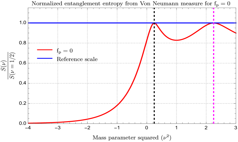
Refer to caption
(a) For fp=0subscript𝑓𝑝0f_{p}=0.
Refer to caption
(b) For small fp0subscript𝑓𝑝0f_{p}\neq 0.
Figure 5.1: Graphical behaviour of the normalized entanglement entropy from Von Neumann measure (S(ν)/S(ν=1/2)𝑆𝜈𝑆𝜈12S(\nu)/S(\nu=1/2)) with mass parameter squared (ν2superscript𝜈2\nu^{2}) for both fp=0subscript𝑓𝑝0f_{p}=0 and small fp0subscript𝑓𝑝0f_{p}\neq 0. Vertical dashed lines are drawn for ν=1/2𝜈12\nu=1/2 (conformally coupled) and ν=3/2𝜈32\nu=3/2 (massless case). In both the plots reference scale corresponds to the scale at which S(ν)/S(ν=1/2)=1𝑆𝜈𝑆𝜈121S(\nu)/S(\nu=1/2)=1.
Refer to caption
(a) For fp=0subscript𝑓𝑝0f_{p}=0.
Refer to caption
(b) For small fp0subscript𝑓𝑝0f_{p}\neq 0.
Figure 5.2: Graphical comparison between the behaviour of the normalized entanglement entropy from Von Neumann measure (S(ν)/S(ν=1/2)𝑆𝜈𝑆𝜈12S(\nu)/S(\nu=1/2)) and normalized entanglement negativity (𝒩(ν)/𝒩(ν=1/2)𝒩𝜈𝒩𝜈12{\cal N}(\nu)/{\cal N}(\nu=1/2)) with mass parameter squared (ν2superscript𝜈2\nu^{2}) for both fp=0subscript𝑓𝑝0f_{p}=0 and small fp0subscript𝑓𝑝0f_{p}\neq 0. Vertical dashed lines are drawn for ν=1/2𝜈12\nu=1/2 (conformally coupled) and ν=3/2𝜈32\nu=3/2 (massless case). In both the plots reference scale corresponds to the scale at which 𝒩(ν)/𝒩(ν=1/2)=1𝒩𝜈𝒩𝜈121{\cal N}(\nu)/{\cal N}(\nu=1/2)=1 and S(ν)/S(ν=1/2)=1𝑆𝜈𝑆𝜈121S(\nu)/S(\nu=1/2)=1.

In this section we give a clear comparison between entanglement entropy and logarithmic negativity, where we know both of them is used to describe the long range quantum correlation and entanglement effects in the present information theory motivated quantum field theoretic picture.

Let us start our discussion with the entanglement entropy which is described by Von Neumann measure by the following expression [14]:

S(p,ν)𝑆𝑝𝜈\displaystyle S(p,\nu) =\displaystyle= 𝐓𝐫[ρ𝐋lnρ𝐋]𝐓𝐫delimited-[]subscript𝜌𝐋subscript𝜌𝐋\displaystyle-{\rm\bf Tr}\left[\rho_{\bf L}\ln\rho_{\bf L}\right] (5.1)
=\displaystyle= {(1+fp1+fp)[ln(1|γp|2)+|γp|2(1|γp|2)ln(|γp|2)]\displaystyle\Bigg{\{}-\left(1+\frac{f_{p}}{1+f_{p}}\right)\left[\ln\left(1-|\gamma_{p}|^{2}\right)+\frac{|\gamma_{p}|^{2}}{\left(1-|\gamma_{p}|^{2}\right)}\ln\left(|\gamma_{p}|^{2}\right)\right]
(1fp)ln(1+fp)},\displaystyle\quad\quad\quad\quad\quad\quad\quad\quad\quad\quad\quad\quad\quad\quad\quad\quad\quad\quad\quad-\left(1-f_{p}\right)\ln\left(1+f_{p}\right)\Bigg{\}},

where we have computed each explicit parameter in the earlier section of this study, together with the explicit expression for the reduced density matrix.

Now by following the same prescription stated before the regularized part of the entanglement entropy can be further expressed by the following simplified expression:

S(ν)𝑆𝜈\displaystyle S(\nu) =\displaystyle= V𝐇𝟑𝐫𝐞𝐠0𝑑p𝒟(p)S(p,ν)=1π0𝑑pp2S(p,ν),subscriptsuperscript𝑉𝐫𝐞𝐠superscript𝐇3subscriptsuperscript0differential-d𝑝𝒟𝑝𝑆𝑝𝜈1𝜋subscriptsuperscript0differential-d𝑝superscript𝑝2𝑆𝑝𝜈\displaystyle V^{\bf reg}_{\bf H^{3}}\int^{\infty}_{0}\leavevmode\nobreak\ dp\leavevmode\nobreak\ {\cal D}(p)\leavevmode\nobreak\ S(p,\nu)=\frac{1}{\pi}\int^{\infty}_{0}\leavevmode\nobreak\ dp\leavevmode\nobreak\ p^{2}\leavevmode\nobreak\ S(p,\nu), (5.2)

where 𝒟(p)𝒟𝑝{\cal D}(p) and V𝐇𝟑𝐫𝐞𝐠subscriptsuperscript𝑉𝐫𝐞𝐠superscript𝐇3V^{\bf reg}_{\bf H^{3}} are defined earlier. Further applying the same logical argument with the UV cut off for the computational purpose we further use the following UV cut off regulated version of Von Neumann entropy:

S(ν)𝑆𝜈\displaystyle S(\nu) =\displaystyle= 1π0Λ𝑑pp2S(p,ν).1𝜋subscriptsuperscriptΛ0differential-d𝑝superscript𝑝2𝑆𝑝𝜈\displaystyle\frac{1}{\pi}\int^{\Lambda}_{0}\leavevmode\nobreak\ dp\leavevmode\nobreak\ p^{2}\leavevmode\nobreak\ S(p,\nu). (5.3)

Our next job is to numerically compute the expressions for entanglement entropy from the above mentioned UV regulated Von Neumann measure which will going to be extremely useful for the further comparison purpose with the results obtained from logarithmic negativity and entanglement negativity measures.

In figure (5.1(a)) and figure (5.1(b)), we have explicitly depicted the behaviour of normalized entanglement entropy from Von Neumann measure (S(ν)/S(ν=1/2)𝑆𝜈𝑆𝜈12S(\nu)/S(\nu=1/2)) with mass parameter squared (ν2superscript𝜈2\nu^{2}) for both fp=0subscript𝑓𝑝0f_{p}=0 and small fp0subscript𝑓𝑝0f_{p}\neq 0. Similarly, in figure (5.2(a)) and figure (5.2(b)), we have explicitly plotted comparative behaviour between normalized entanglement negativity (𝒩(ν)/𝒩(ν=1/2)𝒩𝜈𝒩𝜈12{\cal N}(\nu)/{\cal N}(\nu=1/2)) and normalized entanglement entropy from Von Neumann measure (S(ν)/S(ν=1/2)𝑆𝜈𝑆𝜈12S(\nu)/S(\nu=1/2)) with mass parameter squared (ν2superscript𝜈2\nu^{2}) for both fp=0subscript𝑓𝑝0f_{p}=0 and small fp0subscript𝑓𝑝0f_{p}\neq 0. Vertical dashed lines are drawn for ν=1/2𝜈12\nu=1/2 and ν=3/2𝜈32\nu=3/2 (Case A) cases. In both the plots we have drawn a horizon line at 𝒩(ν)/𝒩(ν=1/2)=1𝒩𝜈𝒩𝜈121{\cal N}(\nu)/{\cal N}(\nu=1/2)=1 and S(ν)/S(ν=1/2)=1𝑆𝜈𝑆𝜈121S(\nu)/S(\nu=1/2)=1 to indicate the reference level of our computation. The outcomes and the physical interpretation of these plots are very interesting which we are writing point-wise in the following:

  1. 1.

    From all of these plots we found that compared entanglement entropy computed from Von Neumann measure entanglement negativity give more information from the same system under consideration. The reason behind this statement is both in the heavy mass ν2<0superscript𝜈20\nu^{2}<0 and small mass ν2>0superscript𝜈20\nu^{2}>0 regions we get more amplitude from the normalized version of the information content.

  2. 2.

    In the heavy mass ν2<0superscript𝜈20\nu^{2}<0 region we found that in the asymptotic limit entanglement entropy gives vanishing contribution, but in the same limit entanglement negativity gives small but significantly non vanishing contribution. On the other hand, in the small mass ν2>0superscript𝜈20\nu^{2}>0 region the amplitude of fluctuation of normalized entanglement entropy is larger amplitude than the normalized entanglement negativity.

  3. 3.

    Only at ν=1/2𝜈12\nu=1/2 (conformally coupled) and ν=3/2𝜈32\nu=3/2 (massless) we get exactly same contribution from both 𝒩(ν)/𝒩(ν=1/2)𝒩𝜈𝒩𝜈12{\cal N}(\nu)/{\cal N}(\nu=1/2) and S(ν)/S(ν=1/2)𝑆𝜈𝑆𝜈12S(\nu)/S(\nu=1/2), which is exactly 𝒩(ν)/𝒩(ν=1/2)=S(ν)/S(ν=1/2)=1𝒩𝜈𝒩𝜈12𝑆𝜈𝑆𝜈121{\cal N}(\nu)/{\cal N}(\nu=1/2)=S(\nu)/S(\nu=1/2)=1.

This is obviously a very interesting finding from our analysis that in case of the present quantum field theoretic set up entanglement negativity captures better information regarding quantum mechanical correlations and quantum entanglement than the Von Neumann measure of entanglement entropy.

6 Logarithmic negativity between two causally unrelated patches of open chart

Our main goal in this part is to calculate and estimate the logarithmic negativity between two patches of the open chart of the global de Sitter space that are not causally related. We provide information on two physical observers whose role it is to explicitly determine and estimate the quantum mechanical entanglement in the current theoretical setup in order to serve the goal. For the purpose of computational simplification, we additionally assume that the quantum states corresponding to these two observers constitute an initial pure state within the multiverse and are maximally entangled to one another.Since we are dealing with two observers, the corresponding framework in a more simpler language can be interpreted as biverse which can be easily further generalise to a general multiverse scenario. From the starting point of the present construction we have explicitly mentioned that the sub regions R and L in the penrose diagram as well as in the Hilbert space construction is taken to be completely symmetric. For this reason to extend this theoretical tool to compute the entanglement negativity from the corresponding biverse set up we consider that the region L is in the inside of the de Sitter bubble. One can do the similar thing by making use of the region R as well. Another important assumption we have considered during this computation is that there is no bubble wall exists in this framework for the open chart of the global de Sitter space. Further in this biverse set up we place another observer in the other open chart of the global de Sitter bubble. From the present theoretical computation our objective is to explicitly find the role of the inside observer to detect the quantum mechanical signatures of entanglement between two de Sitter bubbles using the well known Bunch Davies initial quantum states for the biverse. Now in the present quantum field theoretic set up causality demands that the region R has to be causally unrelated from the other region L. This is because of the fact that there is no access to the region R during this computation. For this specific reason one needs to consider the partial trace operation over the inaccessible region R, which further give rise to the information loss regarding this specific region. As a consequence the corresponding quantum mechanical state which describe the observer would be a mixed quantum state for this computation. In this set up the quantum mechanical state associated with the other observer becomes a pure quantum state which belongs to the other causally unrelated patch of the open chart of the global de Sitter bubble. This implies in the present computation we need to consider the entanglement between a mixed and pure quantum mechanical states which belong to two causally unrelated de Sitter bubbles. If in the computation of quantum entanglement from two subsystems only pure quantum states are involved then in such a system Von Neumann measure is the best measure to quantify entanglement entropy. But if any of the subsystem is described by mixed quantum state then for such a situation Von Neumann measure is not the appropriate quantum information theoretic measure. In that case entanglement negativity or the logarithmic negativity can give better measure of quantum entanglement, which is somewhat clear to us from the comparison that we have already drawn from our previous analysis. He strongly believe that this new measure will going to explain various unexplored underlying physics involved in the present theoretical set up.

6.1 Computational set up and construction of maximally entangled states

Starting with the total quantum vacuum state, which is actually represented by the product of the quantum vacuum states for each oscillator that we found computed explicitly in the previous section of this paper, we begin to study the effects from entanglement negativity between two causally unrelated patches of open chart. It’s crucial to remember that each oscillator’s quantum mechanical state is identified by one of the three quantum numbers p𝑝p, l𝑙l, or m𝑚m for future calculation purposes. For this reason, one must take product over p𝑝p in the final expression of total quantum. The final Bunch Davies quantum vacuum state in this configuration is stated as:

|0𝐁𝐃subscriptket0𝐁𝐃\displaystyle|0\rangle_{\bf BD} =\displaystyle= p|0p𝐁𝐃,subscriptproduct𝑝subscriptketsubscript0𝑝𝐁𝐃\displaystyle\prod_{p}|0_{p}\rangle_{\bf BD}, (6.1)

where we define the Bunch Davies states for each mode as:

|0p𝐁𝐃subscriptketsubscript0𝑝𝐁𝐃\displaystyle|0_{p}\rangle_{\bf BD} =\displaystyle= {(1|γp|2)(1+fp)k=0|γp|k(|kp𝐑|kp𝐋)\displaystyle\Bigg{\{}\sqrt{\frac{\left(1-|\gamma_{p}|^{2}\right)}{\left(1+f_{p}\right)}}\sum^{\infty}_{k=0}|\gamma_{p}|^{k}\bigg{(}|k_{p}\rangle_{{\bf R}^{{}^{\prime}}}\otimes|k_{p}\rangle_{{\bf L}^{{}^{\prime}}}\bigg{)} (6.2)
+fp(1+fp)n=0r=0|Γp,n|r(|n,rp𝐑|n,rp𝐋)}.\displaystyle\quad\quad\quad\quad\quad\quad+\frac{f_{p}}{\sqrt{\left(1+f_{p}\right)}}\sum^{\infty}_{n=0}\sum^{\infty}_{r=0}|\Gamma_{p,n}|^{r}\bigg{(}|n,r_{p}\rangle_{{\bf R}^{{}^{\prime}}}\otimes|n,r_{p}\rangle_{{\bf L}^{{}^{\prime}}}\bigg{)}\Bigg{\}}.\leavevmode\nobreak\ \leavevmode\nobreak\ \leavevmode\nobreak\ \leavevmode\nobreak\ \leavevmode\nobreak\ \leavevmode\nobreak\ \leavevmode\nobreak\ \leavevmode\nobreak\ \leavevmode\nobreak\ \quad

Here it is important to note that, in the above expression for the simplification in the writing purpose we have removed the tags of l𝑙l and m𝑚m on the individual direct product states defined in the region R and L in the Bogoliubov transformed basis. This simplification will going to further help us to deal with cumbersome expressions.

In this specific computation we are actually considering smaller version of the multiverse where many causally unrelated patches in the open chart of the de Sitter bubbles forms a maximally entangled state which is necessary ingredient for the present calculation. In this calculation it is assumed that each of the causally unrelated patches corresponds to a Bunch Davies quantum vacuum states which will finally form a maximally entangled state out of all possible Bunch Davies states. However this is not a strict assumption to extract the required outcome from the present computational set up. One can think about a scenario in which some quantum vacuum states are distinct from Bunch Davies vacuum and are entangled with one another in a more general version of the computation. This is quite an interesting possibility in this context. Now we don’t want to complicate our understanding at this level of computation. For this reason we are going to restrict our analysis by considering the two Bunch Davies quantum vacuum states which belong to two causally unrelated patches of the open chart of the de Sitter bubbles. Now to theoretically model the present computational set up let us first consider two momentum modes having momenta p=p𝐢𝐧𝑝subscript𝑝𝐢𝐧p=p_{\bf in} and p=p𝐨𝐮𝐭𝑝subscript𝑝𝐨𝐮𝐭p=p_{\bf out} of the axionic field theory described by Case A (massless) and Case B (massive) respectively. With this knowledge, it is possible to further express the maximally entangled state in terms of the unique contributions of Bunch Davies vacuum to the two causally independent regions of the de Sitter bubbles as follows:

|Ψ𝐌𝐄::subscriptketΨ𝐌𝐄absent\displaystyle|\Psi\rangle_{\bf ME}: =\displaystyle= 12i=0,1(|ip𝐨𝐮𝐭𝐁𝐃𝟏|ip𝐢𝐧𝐁𝐃𝟐)12subscript𝑖01tensor-productsubscriptketsubscript𝑖subscript𝑝𝐨𝐮𝐭subscript𝐁𝐃1subscriptketsubscript𝑖subscript𝑝𝐢𝐧subscript𝐁𝐃2\displaystyle\frac{1}{\sqrt{2}}\sum_{i=0,1}\Bigg{(}|i_{p_{\bf out}}\rangle_{\bf BD_{1}}\otimes|i_{p_{\bf in}}\rangle_{\bf BD_{2}}\Bigg{)} (6.3)
=\displaystyle= 12(|0p𝐨𝐮𝐭𝐁𝐃𝟏|0p𝐢𝐧𝐁𝐃𝟐+|1p𝐨𝐮𝐭𝐁𝐃𝟏|1p𝐢𝐧𝐁𝐃𝟐).12tensor-productsubscriptketsubscript0subscript𝑝𝐨𝐮𝐭subscript𝐁𝐃1subscriptketsubscript0subscript𝑝𝐢𝐧subscript𝐁𝐃2tensor-productsubscriptketsubscript1subscript𝑝𝐨𝐮𝐭subscript𝐁𝐃1subscriptketsubscript1subscript𝑝𝐢𝐧subscript𝐁𝐃2\displaystyle\frac{1}{\sqrt{2}}\Bigg{(}|0_{p_{\bf out}}\rangle_{\bf BD_{1}}\otimes|0_{p_{\bf in}}\rangle_{\bf BD_{2}}+|1_{p_{\bf out}}\rangle_{\bf BD_{1}}\otimes|1_{p_{\bf in}}\rangle_{\bf BD_{2}}\Bigg{)}.
Refer to caption
Figure 6.1: Representative diagram of the Hilbert space factorization of the axionic biverse which is constructed out of two de Sitter vacua. Each of the vacua is spanned in terms of the complete set of Bunch Davies states.

In the above equation, |0p𝐨𝐮𝐭𝐁𝐃𝟏subscriptketsubscript0subscript𝑝𝐨𝐮𝐭subscript𝐁𝐃1|0_{p_{\bf out}}\rangle_{\bf BD_{1}} and |1p𝐨𝐮𝐭𝐁𝐃𝟏subscriptketsubscript1subscript𝑝𝐨𝐮𝐭subscript𝐁𝐃1|1_{p_{\bf out}}\rangle_{\bf BD_{1}} represent the ground and first single particle excited quantum state characterized by the momentum mode p𝐨𝐮𝐭subscript𝑝𝐨𝐮𝐭p_{\bf out} in the first Bunch Davies vacuum obtained from the first patch of the open chart of global the de Sitter space. Similarly, |0p𝐢𝐧𝐁𝐃𝟐subscriptketsubscript0subscript𝑝𝐢𝐧subscript𝐁𝐃2|0_{p_{\bf in}}\rangle_{\bf BD_{2}} and |1p𝐢𝐧𝐁𝐃𝟐subscriptketsubscript1subscript𝑝𝐢𝐧subscript𝐁𝐃2|1_{p_{\bf in}}\rangle_{\bf BD_{2}} represent the ground and first single particle excited quantum state characterized by the momentum mode p𝐢𝐧subscript𝑝𝐢𝐧p_{\bf in} in the second Bunch Davies vacuum obtained from the second patch of the open chart of global the de Sitter space. For the further computational simplification purpose we assume that outside and inside observers are associated with two detectors having mode momenta p𝐨𝐮𝐭subscript𝑝𝐨𝐮𝐭p_{\bf out} and p𝐢𝐧subscript𝑝𝐢𝐧p_{\bf in} respectively. It is also crucial to note that, given the current quantum field theoretic framework, the complete Hilbert space can be factored as follows:

:=(𝐁𝐃𝟏𝐁𝐃𝟐)=((𝐋𝐇𝐑)𝐁𝐃𝟏𝐅𝐨𝐫𝐟𝐢𝐫𝐬𝐭𝐬𝐮𝐛𝐬𝐩𝐚𝐜𝐞(𝐋𝐇𝐑)𝐁𝐃𝟐𝐅𝐨𝐫𝐬𝐞𝐜𝐨𝐧𝐝𝐬𝐮𝐛𝐬𝐩𝐚𝐜𝐞),assigntensor-productsubscriptsubscript𝐁𝐃1subscriptsubscript𝐁𝐃2tensor-productsubscriptsubscripttensor-productsubscript𝐋subscript𝐇𝐑subscript𝐁𝐃1𝐅𝐨𝐫𝐟𝐢𝐫𝐬𝐭𝐬𝐮𝐛𝐬𝐩𝐚𝐜𝐞subscriptsubscripttensor-productsubscript𝐋subscript𝐇𝐑subscript𝐁𝐃2𝐅𝐨𝐫𝐬𝐞𝐜𝐨𝐧𝐝𝐬𝐮𝐛𝐬𝐩𝐚𝐜𝐞\displaystyle{\cal H}:=\bigg{(}{\cal H}_{\bf{BD}_{1}}\otimes{\cal H}_{\bf{BD}_{2}}\bigg{)}=\Bigg{(}\underbrace{\bigg{(}{\cal H}_{\bf L}\otimes{\bf H}_{\bf R}\bigg{)}_{\bf{BD}_{1}}}_{\bf For\leavevmode\nobreak\ first\leavevmode\nobreak\ subspace}\otimes\underbrace{\bigg{(}{\cal H}_{\bf L}\otimes{\bf H}_{\bf R}\bigg{)}_{\bf{BD}_{2}}}_{\bf For\leavevmode\nobreak\ second\leavevmode\nobreak\ subspace}\Bigg{)}, (6.4)

where the first and the second Bunch Davies vacuum states are associated with two subspace, whose corresponding product Hilbert space can be further factorized in terms Hilbert spaces associated with region R and L as:

𝐁𝐃𝟏subscriptsubscript𝐁𝐃1\displaystyle{\cal H}_{\bf{BD}_{1}} =\displaystyle= (𝐋𝐇𝐑)𝐁𝐃𝟏,subscripttensor-productsubscript𝐋subscript𝐇𝐑subscript𝐁𝐃1\displaystyle\bigg{(}{\cal H}_{\bf L}\otimes{\bf H}_{\bf R}\bigg{)}_{\bf{BD}_{1}}, (6.5)
𝐁𝐃𝟐subscriptsubscript𝐁𝐃2\displaystyle{\cal H}_{\bf{BD}_{2}} =\displaystyle= (𝐋𝐇𝐑)𝐁𝐃𝟐.subscripttensor-productsubscript𝐋subscript𝐇𝐑subscript𝐁𝐃2\displaystyle\bigg{(}{\cal H}_{\bf L}\otimes{\bf H}_{\bf R}\bigg{)}_{\bf{BD}_{2}}. (6.6)

In the multiverse picture one can further generalize this result y considering many Bunch Davies states and different quantum vacua than Bunch Davies, such as α𝛼\alpha vacua, Motta Allen vacua etc. In figure (6.1) representative diagram of the Hilbert space factorization of the axionic biverse which is constructed out of two de Sitter vacua. Each of the vacua is spanned in terms of the complete set of Bunch Davies states which we have pointed clearly in this diagram.

6.2 Construction of excited quantum state for single oscillator

Our main task in this paragraph is to create the excited quantum state for a single oscillator, which will also be helpful to create the overall maximally entangled state required for the specific computation. Let’s start with the characteristic matrix equation for the oscillators in the recently announced Bogoliubov transformed basis to demonstrate this issue in more detail:

cJsubscript𝑐𝐽\displaystyle c_{J} =\displaystyle= bI𝒢JI,CJ(n)=b¯J(n)(𝒢(n))JIwherecJ=(cq,cq),CJ(n)=(Cq(n),Cq(n)),formulae-sequencesubscript𝑏𝐼subscriptsuperscript𝒢𝐼𝐽subscript𝐶𝐽𝑛subscript¯𝑏𝐽𝑛subscriptsuperscriptsubscript𝒢𝑛𝐼𝐽wheresubscript𝑐𝐽subscript𝑐𝑞subscriptsuperscript𝑐𝑞subscript𝐶𝐽𝑛subscript𝐶𝑞𝑛subscriptsuperscript𝐶𝑞𝑛\displaystyle b_{I}{\cal G}^{I}_{J},\leavevmode\nobreak\ \quad C_{J(n)}=\bar{b}_{J(n)}\left({\cal G}_{(n)}\right)^{I}_{J}\quad\quad{\rm where}\quad\quad c_{J}=(c_{q},c^{\dagger}_{q}),C_{J(n)}=(C_{q(n)},C^{\dagger}_{q(n)}),\quad\quad\quad (6.7)

where we define the two square matrices as appearing in the above expressions by the following equations:

𝒢JI=(UqVqVqUq),(𝒢(n))JI=(U¯q,nV¯σq,nV¯q,nU¯q,n),formulae-sequencesubscriptsuperscript𝒢𝐼𝐽subscript𝑈𝑞subscriptsuperscript𝑉𝑞missing-subexpressionsubscript𝑉𝑞subscriptsuperscript𝑈𝑞missing-subexpressionsubscriptsuperscriptsubscript𝒢𝑛𝐼𝐽subscript¯𝑈𝑞𝑛subscriptsuperscript¯𝑉𝜎𝑞𝑛missing-subexpressionsubscript¯𝑉𝑞𝑛subscriptsuperscript¯𝑈𝑞𝑛missing-subexpression\displaystyle{\cal G}^{I}_{J}=\left(\begin{array}[]{ccc}U_{q}&\leavevmode\nobreak\ \leavevmode\nobreak\ \leavevmode\nobreak\ V^{*}_{q}\\ V_{q}&\leavevmode\nobreak\ \leavevmode\nobreak\ \leavevmode\nobreak\ U^{*}_{q}\end{array}\right),\leavevmode\nobreak\ \quad\quad\left({\cal G}_{(n)}\right)^{I}_{J}=\left(\begin{array}[]{ccc}\overline{U}_{q,n}&\leavevmode\nobreak\ \leavevmode\nobreak\ \leavevmode\nobreak\ \overline{V}^{*}_{\sigma q,n}\\ \overline{V}_{q,n}&\leavevmode\nobreak\ \leavevmode\nobreak\ \leavevmode\nobreak\ \overline{U}^{*}_{q,n}\end{array}\right),\quad\quad\quad\quad (6.12)

where the components of the new matrices are given by:

Uqsubscript𝑈𝑞\displaystyle U_{q} \displaystyle\equiv 𝐝𝐢𝐚𝐠(u,u¯),𝐝𝐢𝐚𝐠𝑢¯𝑢\displaystyle{\rm\bf diag}\left(u,\overline{u}\right), (6.13)
Vqsubscript𝑉𝑞\displaystyle V_{q} \displaystyle\equiv 𝐝𝐢𝐚𝐠(v,v¯),𝐝𝐢𝐚𝐠𝑣¯𝑣\displaystyle{\rm\bf diag}\left(v,\overline{v}\right), (6.14)
U¯q,nsubscript¯𝑈𝑞𝑛\displaystyle\overline{U}_{q,n} \displaystyle\equiv 𝐝𝐢𝐚𝐠(Un,U¯n),𝐝𝐢𝐚𝐠subscript𝑈𝑛subscript¯𝑈𝑛\displaystyle{\rm\bf diag}\left(U_{n},\overline{U}_{n}\right), (6.15)
V¯q,nsubscript¯𝑉𝑞𝑛\displaystyle\overline{V}_{q,n} \displaystyle\equiv 𝐝𝐢𝐚𝐠(Vn,V¯n).𝐝𝐢𝐚𝐠subscript𝑉𝑛subscript¯𝑉𝑛\displaystyle{\rm\bf diag}\left(V_{n},\overline{V}_{n}\right). (6.16)

Hence one can able to find the relationship between the a𝑎a-type of oscillators with c-type of oscillators, which are given by:

aJ(c)subscriptsuperscript𝑎𝑐𝐽\displaystyle a^{(c)}_{J} =\displaystyle= bJ(1)JI=cK(𝒢1)IK(1)JI,subscript𝑏𝐽subscriptsuperscriptsuperscript1𝐼𝐽subscript𝑐𝐾subscriptsuperscriptsuperscript𝒢1𝐾𝐼subscriptsuperscriptsuperscript1𝐼𝐽\displaystyle b_{J}\left({\cal M}^{-1}\right)^{I}_{J}=c_{K}\left({\cal G}^{-1}\right)^{K}_{I}\left({\cal M}^{-1}\right)^{I}_{J}, (6.17)
aJ(n)(p)subscriptsuperscript𝑎𝑝𝐽𝑛\displaystyle a^{(p)}_{J(n)} =\displaystyle= bJ(n)((n)1)JI=CK(n)(𝒢(n)1)IK((n)1)JI,subscript𝑏𝐽𝑛subscriptsuperscriptsubscriptsuperscript1𝑛𝐼𝐽subscript𝐶𝐾𝑛subscriptsuperscriptsubscriptsuperscript𝒢1𝑛𝐾𝐼subscriptsuperscriptsubscriptsuperscript1𝑛𝐼𝐽\displaystyle b_{J(n)}\left({\cal M}^{-1}_{(n)}\right)^{I}_{J}=C_{K(n)}\left({\cal G}^{-1}_{(n)}\right)^{K}_{I}\left({\cal M}^{-1}_{(n)}\right)^{I}_{J}, (6.18)

which further form the following quantity:

aIsubscript𝑎𝐼\displaystyle a_{I} =\displaystyle= [aI(c)+n=0aI(n)(p)]=[cK(𝒢1)IK(1)JI𝐂𝐨𝐦𝐩𝐥𝐞𝐦𝐞𝐧𝐭𝐚𝐫𝐲𝐩𝐚𝐫𝐭+n=0CK(n)(𝒢(n)1)IK((n)1)JI𝐏𝐚𝐫𝐭𝐢𝐜𝐮𝐥𝐚𝐫𝐢𝐧𝐭𝐞𝐠𝐫𝐚𝐥𝐩𝐚𝐫𝐭].delimited-[]subscriptsuperscript𝑎𝑐𝐼subscriptsuperscript𝑛0subscriptsuperscript𝑎𝑝𝐼𝑛delimited-[]subscriptsubscript𝑐𝐾subscriptsuperscriptsuperscript𝒢1𝐾𝐼subscriptsuperscriptsuperscript1𝐼𝐽𝐂𝐨𝐦𝐩𝐥𝐞𝐦𝐞𝐧𝐭𝐚𝐫𝐲𝐩𝐚𝐫𝐭subscriptsubscriptsuperscript𝑛0subscript𝐶𝐾𝑛subscriptsuperscriptsubscriptsuperscript𝒢1𝑛𝐾𝐼subscriptsuperscriptsubscriptsuperscript1𝑛𝐼𝐽𝐏𝐚𝐫𝐭𝐢𝐜𝐮𝐥𝐚𝐫𝐢𝐧𝐭𝐞𝐠𝐫𝐚𝐥𝐩𝐚𝐫𝐭\displaystyle\left[a^{(c)}_{I}+\sum^{\infty}_{n=0}a^{(p)}_{I(n)}\right]=\bigg{[}\underbrace{c_{K}\left({\cal G}^{-1}\right)^{K}_{I}\left({\cal M}^{-1}\right)^{I}_{J}}_{\bf Complementary\leavevmode\nobreak\ part}+\underbrace{\sum^{\infty}_{n=0}C_{K(n)}\left({\cal G}^{-1}_{(n)}\right)^{K}_{I}\left({\cal M}^{-1}_{(n)}\right)^{I}_{J}}_{\bf Particular\leavevmode\nobreak\ integral\leavevmode\nobreak\ part}\bigg{]}.\quad\quad (6.19)

Here the the product of two inverse matrices are parametrized by another (4×4)44(4\times 4) square matrix, which is given by:

(𝒢1)IK(1)JIsubscriptsuperscriptsuperscript𝒢1𝐾𝐼subscriptsuperscriptsuperscript1𝐼𝐽\displaystyle\left({\cal G}^{-1}\right)^{K}_{I}\left({\cal M}^{-1}\right)^{I}_{J} =\displaystyle= (QσqRσqRσqQσq),subscript𝑄𝜎𝑞subscriptsuperscript𝑅𝜎𝑞missing-subexpressionsubscript𝑅𝜎𝑞subscriptsuperscript𝑄𝜎𝑞missing-subexpression\displaystyle\left(\begin{array}[]{ccc}Q_{\sigma q}&\leavevmode\nobreak\ \leavevmode\nobreak\ \leavevmode\nobreak\ R^{*}_{\sigma q}\\ R_{\sigma q}&\leavevmode\nobreak\ \leavevmode\nobreak\ \leavevmode\nobreak\ Q^{*}_{\sigma q}\end{array}\right), (6.22)
(𝒢(n)1)IK((n)1)JIsubscriptsuperscriptsubscriptsuperscript𝒢1𝑛𝐾𝐼subscriptsuperscriptsubscriptsuperscript1𝑛𝐼𝐽\displaystyle\left({\cal G}^{-1}_{(n)}\right)^{K}_{I}\left({\cal M}^{-1}_{(n)}\right)^{I}_{J} =\displaystyle= (Q¯σq,nR¯σq,nRσq,nQ¯σq,n),subscript¯𝑄𝜎𝑞𝑛subscriptsuperscript¯𝑅𝜎𝑞𝑛missing-subexpressionsubscript𝑅𝜎𝑞𝑛subscriptsuperscript¯𝑄𝜎𝑞𝑛missing-subexpression\displaystyle\left(\begin{array}[]{ccc}\overline{Q}_{\sigma q,n}&\leavevmode\nobreak\ \leavevmode\nobreak\ \leavevmode\nobreak\ \overline{R}^{*}_{\sigma q,n}\\ R_{\sigma q,n}&\leavevmode\nobreak\ \leavevmode\nobreak\ \leavevmode\nobreak\ \overline{Q}^{*}_{\sigma q,n}\end{array}\right), (6.25)

where the elements of both the matrices are itself (2×2)22(2\times 2) matrices, which are provided by the subsequent expressions:

Qσqsubscript𝑄𝜎𝑞\displaystyle Q_{\sigma q} =\displaystyle= (A~uB~u+D~vB~u+D~vA~u),~𝐴𝑢~𝐵𝑢superscript~𝐷𝑣missing-subexpression~𝐵𝑢superscript~𝐷𝑣~𝐴𝑢missing-subexpression\displaystyle\left(\begin{array}[]{ccc}\widetilde{A}u\nobreak\leavevmode\nobreak\leavevmode\nobreak\leavevmode&\leavevmode\nobreak\ \leavevmode\nobreak\ \leavevmode\nobreak\ -\widetilde{B}u+\widetilde{D}^{*}v\\ -\widetilde{B}u+\widetilde{D}^{*}v&\leavevmode\nobreak\ \leavevmode\nobreak\ \leavevmode\nobreak\ \widetilde{A}u\end{array}\right), (6.28)
Rσqsubscript𝑅𝜎𝑞\displaystyle R_{\sigma q} =\displaystyle= (A~vB~vD~uB~vD~uA~v),~𝐴𝑣~𝐵𝑣superscript~𝐷𝑢missing-subexpression~𝐵𝑣superscript~𝐷𝑢~𝐴𝑣missing-subexpression\displaystyle\left(\begin{array}[]{ccc}-\widetilde{A}v\nobreak\leavevmode\nobreak\leavevmode\nobreak\leavevmode&\widetilde{B}v-\widetilde{D}^{*}u\\ \widetilde{B}v-\widetilde{D}^{*}u&\leavevmode\nobreak\ \leavevmode\nobreak\ \leavevmode\nobreak\ -\widetilde{A}v\end{array}\right), (6.31)
Qσq,nsubscript𝑄𝜎𝑞𝑛\displaystyle Q_{\sigma q,n} =\displaystyle= (A~nUnB~nUn+D~nVnB~nUn+D~nVnA~nUn),subscript~𝐴𝑛subscript𝑈𝑛subscript~𝐵𝑛subscript𝑈𝑛subscriptsuperscript~𝐷𝑛subscript𝑉𝑛missing-subexpressionsubscript~𝐵𝑛subscript𝑈𝑛subscriptsuperscript~𝐷𝑛subscript𝑉𝑛subscript~𝐴𝑛subscript𝑈𝑛missing-subexpression\displaystyle\left(\begin{array}[]{ccc}\widetilde{A}_{n}U_{n}\nobreak\leavevmode\nobreak\leavevmode\nobreak\leavevmode&\leavevmode\nobreak\ \leavevmode\nobreak\ \leavevmode\nobreak\ -\widetilde{B}_{n}U_{n}+\widetilde{D}^{*}_{n}V_{n}\\ -\widetilde{B}_{n}U_{n}+\widetilde{D}^{*}_{n}V_{n}&\leavevmode\nobreak\ \leavevmode\nobreak\ \leavevmode\nobreak\ \widetilde{A}_{n}U_{n}\end{array}\right), (6.34)
Rσq,nsubscript𝑅𝜎𝑞𝑛\displaystyle R_{\sigma q,n} =\displaystyle= (A~nVnB~nVnD~nUnB~nVnD~nUnA~nVn).subscript~𝐴𝑛subscript𝑉𝑛subscript~𝐵𝑛subscript𝑉𝑛subscriptsuperscript~𝐷𝑛subscript𝑈𝑛missing-subexpressionsubscript~𝐵𝑛subscript𝑉𝑛subscriptsuperscript~𝐷𝑛subscript𝑈𝑛subscript~𝐴𝑛subscript𝑉𝑛missing-subexpression\displaystyle\left(\begin{array}[]{ccc}-\widetilde{A}_{n}V_{n}\nobreak\leavevmode\nobreak\leavevmode\nobreak\leavevmode&\widetilde{B}_{n}V_{n}-\widetilde{D}^{*}_{n}U_{n}\\ \widetilde{B}_{n}V_{n}-\widetilde{D}^{*}_{n}U_{n}&\leavevmode\nobreak\ \leavevmode\nobreak\ \leavevmode\nobreak\ -\widetilde{A}_{n}V_{n}\end{array}\right). (6.37)

Here the coefficients (A~~𝐴\widetilde{A}, B~~𝐵\widetilde{B},D~~𝐷\widetilde{D}) and (A~nsubscript~𝐴𝑛\widetilde{A}_{n}, B~nsubscript~𝐵𝑛\widetilde{B}_{n},D~nsubscript~𝐷𝑛\widetilde{D}_{n}) aare provided by the subsequent expressions:

A~~𝐴\displaystyle\widetilde{A} =\displaystyle= πp|Γ(ν+12+ip)|exp(πp2)cosh2πp+cos2πν,𝜋𝑝Γ𝜈12𝑖𝑝𝜋𝑝22𝜋𝑝2𝜋𝜈\displaystyle\frac{\sqrt{\pi p}}{\left|\Gamma\left(\nu+\frac{1}{2}+ip\right)\right|}\frac{\exp\left(\frac{\pi p}{2}\right)}{\sqrt{\cosh 2\pi p+\cos 2\pi\nu}}, (6.38)
B~~𝐵\displaystyle\widetilde{B} =\displaystyle= A~cosπνisinhπp~𝐴𝜋𝜈𝑖𝜋𝑝\displaystyle\widetilde{A}\leavevmode\nobreak\ \frac{\cos\pi\nu}{i\sinh\pi p} (6.39)
=\displaystyle= πp|Γ(ν+12+ip)|exp(πp2)cosh2πp+cos2πνcosπνisinhπp,𝜋𝑝Γ𝜈12𝑖𝑝𝜋𝑝22𝜋𝑝2𝜋𝜈𝜋𝜈𝑖𝜋𝑝\displaystyle\frac{\sqrt{\pi p}}{\left|\Gamma\left(\nu+\frac{1}{2}+ip\right)\right|}\frac{\exp\left(\frac{\pi p}{2}\right)}{\sqrt{\cosh 2\pi p+\cos 2\pi\nu}}\frac{\cos\pi\nu}{i\sinh\pi p},
D~~𝐷\displaystyle\widetilde{D} =\displaystyle= A~cos(ip+ν)πisinhπpexp(πp)Γ(ν+12+ip)Γ(ν+12ip)~𝐴𝑖𝑝𝜈𝜋𝑖𝜋𝑝𝜋𝑝Γ𝜈12𝑖𝑝Γ𝜈12𝑖𝑝\displaystyle-\widetilde{A}\leavevmode\nobreak\ \frac{\cos(ip+\nu)\pi}{i\sinh\pi p}\exp\left(-\pi p\right)\frac{\Gamma\left(\nu+\frac{1}{2}+ip\right)}{\Gamma\left(\nu+\frac{1}{2}-ip\right)} (6.40)
=\displaystyle= πp|Γ(ν+12+ip)|exp(πp2)cosh2πp+cos2πνcos(ip+ν)πisinhπpΓ(ν+12+ip)Γ(ν+12ip),𝜋𝑝Γ𝜈12𝑖𝑝𝜋𝑝22𝜋𝑝2𝜋𝜈𝑖𝑝𝜈𝜋𝑖𝜋𝑝Γ𝜈12𝑖𝑝Γ𝜈12𝑖𝑝\displaystyle-\frac{\sqrt{\pi p}}{\left|\Gamma\left(\nu+\frac{1}{2}+ip\right)\right|}\frac{\exp\left(-\frac{\pi p}{2}\right)}{\sqrt{\cosh 2\pi p+\cos 2\pi\nu}}\leavevmode\nobreak\ \frac{\cos(ip+\nu)\pi}{i\sinh\pi p}\frac{\Gamma\left(\nu+\frac{1}{2}+ip\right)}{\Gamma\left(\nu+\frac{1}{2}-ip\right)},

and

A~nsubscript~𝐴𝑛\displaystyle\widetilde{A}_{n} =\displaystyle= πpn|Γ(ν+12+ipn)|exp(πpn2)cosh2πpn+cos2πν,𝜋subscript𝑝𝑛Γ𝜈12𝑖subscript𝑝𝑛𝜋subscript𝑝𝑛22𝜋subscript𝑝𝑛2𝜋𝜈\displaystyle\frac{\sqrt{\pi p_{n}}}{\left|\Gamma\left(\nu+\frac{1}{2}+ip_{n}\right)\right|}\frac{\exp\left(\frac{\pi p_{n}}{2}\right)}{\sqrt{\cosh 2\pi p_{n}+\cos 2\pi\nu}}, (6.41)
B~nsubscript~𝐵𝑛\displaystyle\widetilde{B}_{n} =\displaystyle= A~ncosπνisinhπpnsubscript~𝐴𝑛𝜋𝜈𝑖𝜋subscript𝑝𝑛\displaystyle\widetilde{A}_{n}\leavevmode\nobreak\ \frac{\cos\pi\nu}{i\sinh\pi p_{n}} (6.42)
=\displaystyle= πpn|Γ(ν+12+ipn)|exp(πpn2)cosh2πpn+cos2πνcosπνisinhπpn,𝜋subscript𝑝𝑛Γ𝜈12𝑖subscript𝑝𝑛𝜋subscript𝑝𝑛22𝜋subscript𝑝𝑛2𝜋𝜈𝜋𝜈𝑖𝜋subscript𝑝𝑛\displaystyle\frac{\sqrt{\pi p_{n}}}{\left|\Gamma\left(\nu+\frac{1}{2}+ip_{n}\right)\right|}\frac{\exp\left(\frac{\pi p_{n}}{2}\right)}{\sqrt{\cosh 2\pi p_{n}+\cos 2\pi\nu}}\frac{\cos\pi\nu}{i\sinh\pi p_{n}},
D~nsubscript~𝐷𝑛\displaystyle\widetilde{D}_{n} =\displaystyle= A~ncos(ipn+ν)πisinhπpnexp(πpn)Γ(ν+12+ipn)Γ(ν+12ipn)subscript~𝐴𝑛𝑖subscript𝑝𝑛𝜈𝜋𝑖𝜋subscript𝑝𝑛𝜋subscript𝑝𝑛Γ𝜈12𝑖subscript𝑝𝑛Γ𝜈12𝑖subscript𝑝𝑛\displaystyle-\widetilde{A}_{n}\leavevmode\nobreak\ \frac{\cos(ip_{n}+\nu)\pi}{i\sinh\pi p_{n}}\exp\left(-\pi p_{n}\right)\frac{\Gamma\left(\nu+\frac{1}{2}+ip_{n}\right)}{\Gamma\left(\nu+\frac{1}{2}-ip_{n}\right)} (6.43)
=\displaystyle= πpn|Γ(ν+12+ipn)|exp(πpn2)cosh2πpn+cos2πνcos(ipn+ν)πisinhπpnΓ(ν+12+ipn)Γ(ν+12ipn).𝜋subscript𝑝𝑛Γ𝜈12𝑖subscript𝑝𝑛𝜋subscript𝑝𝑛22𝜋subscript𝑝𝑛2𝜋𝜈𝑖subscript𝑝𝑛𝜈𝜋𝑖𝜋subscript𝑝𝑛Γ𝜈12𝑖subscript𝑝𝑛Γ𝜈12𝑖subscript𝑝𝑛\displaystyle-\frac{\sqrt{\pi p_{n}}}{\left|\Gamma\left(\nu+\frac{1}{2}+ip_{n}\right)\right|}\frac{\exp\left(-\frac{\pi p_{n}}{2}\right)}{\sqrt{\cosh 2\pi p_{n}+\cos 2\pi\nu}}\leavevmode\nobreak\ \frac{\cos(ip_{n}+\nu)\pi}{i\sinh\pi p_{n}}\frac{\Gamma\left(\nu+\frac{1}{2}+ip_{n}\right)}{\Gamma\left(\nu+\frac{1}{2}-ip_{n}\right)}.

From the structure of the above mentioned matrices we have found the following characteristics:

  1. 1.

    First of all we have found that for each of the above mentioned matrices the diagonal and off-diagonal elements are same, which implies each of them are symmetric matrices under the matrix transpose operation i.e.

    Qqσ=QσqT=Qσq,subscript𝑄𝑞𝜎subscriptsuperscript𝑄𝑇𝜎𝑞subscript𝑄𝜎𝑞\displaystyle Q_{q\sigma}=Q^{T}_{\sigma q}=Q_{\sigma q}, (6.44)
    Rqσ=Rσq,nT=Rσq,n,subscript𝑅𝑞𝜎subscriptsuperscript𝑅𝑇𝜎𝑞𝑛subscript𝑅𝜎𝑞𝑛\displaystyle R_{q\sigma}=R^{T}_{\sigma q,n}=R_{\sigma q,n}, (6.45)
    Qqσ,n=Qσq,nT=Qσq,n,subscript𝑄𝑞𝜎𝑛subscriptsuperscript𝑄𝑇𝜎𝑞𝑛subscript𝑄𝜎𝑞𝑛\displaystyle Q_{q\sigma,n}=Q^{T}_{\sigma q,n}=Q_{\sigma q,n}, (6.46)
    Rqσ,n=Rσq,nT=Rσq,n.subscript𝑅𝑞𝜎𝑛subscriptsuperscript𝑅𝑇𝜎𝑞𝑛subscript𝑅𝜎𝑞𝑛\displaystyle R_{q\sigma,n}=R^{T}_{\sigma q,n}=R_{\sigma q,n}. (6.47)
  2. 2.

    In the above mentioned expressions we have also used the following relationships to write down the final result in a more simplified and compact format:

    A~=A~,B~=B~,u=u=u¯,v=v=v¯,formulae-sequenceformulae-sequencesuperscript~𝐴~𝐴formulae-sequencesuperscript~𝐵~𝐵superscript𝑢𝑢¯𝑢superscript𝑣𝑣¯𝑣\displaystyle\widetilde{A}^{*}=\widetilde{A},\quad\quad\widetilde{B}^{*}=-\widetilde{B},\quad\quad u^{*}=u=\overline{u},\quad\quad\quad\quad v^{*}=v=\overline{v}, (6.48)
    A~n=A~n,B~n=B~n,Un=Un=U¯n,Vn=Vn=V¯n.formulae-sequenceformulae-sequencesubscriptsuperscript~𝐴𝑛subscript~𝐴𝑛formulae-sequencesubscriptsuperscript~𝐵𝑛subscript~𝐵𝑛subscriptsuperscript𝑈𝑛subscript𝑈𝑛subscript¯𝑈𝑛subscriptsuperscript𝑉𝑛subscript𝑉𝑛subscript¯𝑉𝑛\displaystyle\widetilde{A}^{*}_{n}=\widetilde{A}_{n},\quad\quad\widetilde{B}^{*}_{n}=-\widetilde{B}_{n},\quad\quad U^{*}_{n}=U_{n}=\overline{U}_{n},\quad\quad V^{*}_{n}=V_{n}=\overline{V}_{n}. (6.49)
  3. 3.

    If we set B=0𝐵0B=0 and B~=0~𝐵0\widetilde{B}=0 along with v=0𝑣0v=0 and Vn=0subscript𝑉𝑛0V_{n}=0 correspond to case of conformal coupling (ν=1/2𝜈12\nu=1/2) and the massless theory (ν=3/2𝜈32\nu=3/2).

The following formulas in the region L provide the creation and annihilation operators for oscillators of the a𝑎a type, and fixing this will fix their explicit mathematical structures:

a𝐋::subscriptsuperscript𝑎𝐋absent\displaystyle a^{\dagger}_{\bf L}: =\displaystyle= (A~uc𝐋A~vc𝐋+(B~u+D~v)c𝐑(B~v+D~u)c𝐑)𝐂𝐨𝐦𝐩𝐥𝐞𝐦𝐞𝐧𝐭𝐚𝐫𝐲𝐩𝐚𝐫𝐭subscript~𝐴𝑢subscriptsuperscript𝑐𝐋~𝐴𝑣subscript𝑐𝐋~𝐵𝑢~𝐷𝑣subscriptsuperscript𝑐𝐑~𝐵𝑣~𝐷𝑢subscript𝑐𝐑𝐂𝐨𝐦𝐩𝐥𝐞𝐦𝐞𝐧𝐭𝐚𝐫𝐲𝐩𝐚𝐫𝐭\displaystyle\underbrace{\Bigg{(}\widetilde{A}uc^{\dagger}_{\bf L}-\widetilde{A}vc_{\bf L}+\left(\widetilde{B}u+\widetilde{D}v\right)c^{\dagger}_{\bf R}-\left(\widetilde{B}v+\widetilde{D}u\right)c_{\bf R}\Bigg{)}}_{\bf Complementary\leavevmode\nobreak\ part}
+n=0(A~nUnC𝐋(n)A~nVnC𝐋(n)+(B~nUn+D~nVn)C𝐑(n)(B~nVn+D~nUn)C𝐑(n))𝐏𝐚𝐫𝐭𝐢𝐜𝐮𝐥𝐚𝐫𝐢𝐧𝐭𝐞𝐠𝐫𝐚𝐥𝐩𝐚𝐫𝐭,subscriptsubscriptsuperscript𝑛0subscript~𝐴𝑛subscript𝑈𝑛subscriptsuperscript𝐶𝐋𝑛subscript~𝐴𝑛subscript𝑉𝑛subscript𝐶𝐋𝑛subscript~𝐵𝑛subscript𝑈𝑛subscript~𝐷𝑛subscript𝑉𝑛subscriptsuperscript𝐶𝐑𝑛subscript~𝐵𝑛subscript𝑉𝑛subscript~𝐷𝑛subscript𝑈𝑛subscript𝐶𝐑𝑛𝐏𝐚𝐫𝐭𝐢𝐜𝐮𝐥𝐚𝐫𝐢𝐧𝐭𝐞𝐠𝐫𝐚𝐥𝐩𝐚𝐫𝐭\displaystyle\quad\quad+\underbrace{\sum^{\infty}_{n=0}\Bigg{(}\widetilde{A}_{n}U_{n}C^{\dagger}_{{\bf L}(n)}-\widetilde{A}_{n}V_{n}C_{{\bf L}(n)}+\left(\widetilde{B}_{n}U_{n}+\widetilde{D}_{n}V_{n}\right)C^{\dagger}_{{\bf R}(n)}-\left(\widetilde{B}_{n}V_{n}+\widetilde{D}_{n}U_{n}\right)C_{{\bf R}(n)}\Bigg{)}}_{\bf Particular\leavevmode\nobreak\ integral\leavevmode\nobreak\ part},
a𝐋::subscript𝑎𝐋absent\displaystyle a_{\bf L}: =\displaystyle= (A~uc𝐋A~vc𝐋+(B~u+D~v)c𝐑(B~v+D~u)c𝐑)𝐂𝐨𝐦𝐩𝐥𝐞𝐦𝐞𝐧𝐭𝐚𝐫𝐲𝐩𝐚𝐫𝐭subscript~𝐴𝑢subscript𝑐𝐋~𝐴𝑣subscriptsuperscript𝑐𝐋~𝐵𝑢superscript~𝐷𝑣subscript𝑐𝐑~𝐵𝑣superscript~𝐷𝑢subscriptsuperscript𝑐𝐑𝐂𝐨𝐦𝐩𝐥𝐞𝐦𝐞𝐧𝐭𝐚𝐫𝐲𝐩𝐚𝐫𝐭\displaystyle\underbrace{\Bigg{(}\widetilde{A}uc_{\bf L}-\widetilde{A}vc^{\dagger}_{\bf L}+\left(-\widetilde{B}u+\widetilde{D}^{*}v\right)c_{\bf R}-\left(-\widetilde{B}v+\widetilde{D}^{*}u\right)c^{\dagger}_{\bf R}\Bigg{)}}_{\bf Complementary\leavevmode\nobreak\ part}
+n=0(A~nUnC𝐋(n)A~nVnC𝐋(n)+(B~nUn+D~nVn)C𝐑(n)(B~nVn+D~nUn)C𝐑(n))𝐏𝐚𝐫𝐭𝐢𝐜𝐮𝐥𝐚𝐫𝐢𝐧𝐭𝐞𝐠𝐫𝐚𝐥𝐩𝐚𝐫𝐭,subscriptsubscriptsuperscript𝑛0subscript~𝐴𝑛subscript𝑈𝑛subscript𝐶𝐋𝑛subscript~𝐴𝑛subscript𝑉𝑛subscriptsuperscript𝐶𝐋𝑛subscript~𝐵𝑛subscript𝑈𝑛subscriptsuperscript~𝐷𝑛subscript𝑉𝑛subscript𝐶𝐑𝑛subscript~𝐵𝑛subscript𝑉𝑛subscriptsuperscript~𝐷𝑛subscript𝑈𝑛subscriptsuperscript𝐶𝐑𝑛𝐏𝐚𝐫𝐭𝐢𝐜𝐮𝐥𝐚𝐫𝐢𝐧𝐭𝐞𝐠𝐫𝐚𝐥𝐩𝐚𝐫𝐭\displaystyle\quad\quad+\underbrace{\sum^{\infty}_{n=0}\Bigg{(}\widetilde{A}_{n}U_{n}C_{{\bf L}(n)}-\widetilde{A}_{n}V_{n}C^{\dagger}_{{\bf L}(n)}+\left(-\widetilde{B}_{n}U_{n}+\widetilde{D}^{\dagger}_{n}V_{n}\right)C_{{\bf R}(n)}-\left(-\widetilde{B}_{n}V_{n}+\widetilde{D}^{\dagger}_{n}U_{n}\right)C^{\dagger}_{{\bf R}(n)}\Bigg{)}}_{\bf Particular\leavevmode\nobreak\ integral\leavevmode\nobreak\ part},

The following expression represents the excited quantum state for a single oscillator and corresponds to the quantum state of the inside observer:

|1p𝐢𝐧𝐁𝐃𝟐subscriptketsubscript1subscript𝑝𝐢𝐧subscript𝐁𝐃2\displaystyle|1_{p_{\bf in}}\rangle_{{\bf BD_{2}}} =\displaystyle= a𝐋|0p𝐢𝐧𝐁𝐃𝟐subscriptsuperscript𝑎𝐋subscriptketsubscript0subscript𝑝𝐢𝐧subscript𝐁𝐃2\displaystyle a^{\dagger}_{\bf L}|0_{p_{\bf in}}\rangle_{{\bf BD_{2}}} (6.52)
=\displaystyle= {(A~uc𝐋A~vc𝐋+(B~u+D~v)c𝐑(B~v+D~u)c𝐑)𝐂𝐨𝐦𝐩𝐥𝐞𝐦𝐞𝐧𝐭𝐚𝐫𝐲𝐩𝐚𝐫𝐭\displaystyle\Bigg{\{}\underbrace{\Bigg{(}\widetilde{A}uc^{\dagger}_{\bf L}-\widetilde{A}vc_{\bf L}+\left(\widetilde{B}u+\widetilde{D}v\right)c^{\dagger}_{\bf R}-\left(\widetilde{B}v+\widetilde{D}u\right)c_{\bf R}\Bigg{)}}_{\bf Complementary\leavevmode\nobreak\ part}
+n=0(A~nUnC𝐋(n)A~nVnC𝐋(n)+(B~nUn+D~nVn)C𝐑(n)(B~nVn+D~nUn)C𝐑(n))𝐏𝐚𝐫𝐭𝐢𝐜𝐮𝐥𝐚𝐫𝐢𝐧𝐭𝐞𝐠𝐫𝐚𝐥𝐩𝐚𝐫𝐭subscriptsubscriptsuperscript𝑛0subscript~𝐴𝑛subscript𝑈𝑛subscriptsuperscript𝐶𝐋𝑛subscript~𝐴𝑛subscript𝑉𝑛subscript𝐶𝐋𝑛subscript~𝐵𝑛subscript𝑈𝑛subscript~𝐷𝑛subscript𝑉𝑛subscriptsuperscript𝐶𝐑𝑛subscript~𝐵𝑛subscript𝑉𝑛subscript~𝐷𝑛subscript𝑈𝑛subscript𝐶𝐑𝑛𝐏𝐚𝐫𝐭𝐢𝐜𝐮𝐥𝐚𝐫𝐢𝐧𝐭𝐞𝐠𝐫𝐚𝐥𝐩𝐚𝐫𝐭\displaystyle+\underbrace{\sum^{\infty}_{n=0}\Bigg{(}\widetilde{A}_{n}U_{n}C^{\dagger}_{{\bf L}(n)}-\widetilde{A}_{n}V_{n}C_{{\bf L}(n)}+\left(\widetilde{B}_{n}U_{n}+\widetilde{D}_{n}V_{n}\right)C^{\dagger}_{{\bf R}(n)}-\left(\widetilde{B}_{n}V_{n}+\widetilde{D}_{n}U_{n}\right)C_{{\bf R}(n)}\Bigg{)}}_{\bf Particular\leavevmode\nobreak\ integral\leavevmode\nobreak\ part}
}{(1|γp𝐢𝐧|2)(1+fp𝐢𝐧)k=0|γp𝐢𝐧|k(|kp𝐢𝐧𝐑|kp𝐢𝐧𝐋)\displaystyle\quad\quad\quad\quad\quad\Bigg{\}}\Bigg{\{}\sqrt{\frac{\left(1-|\gamma_{p_{\bf in}}|^{2}\right)}{\left(1+f_{p_{\bf in}}\right)}}\sum^{\infty}_{k=0}|\gamma_{p_{\bf in}}|^{k}\bigg{(}|k_{p_{\bf in}}\rangle_{{\bf R}^{{}^{\prime}}}\otimes|k_{p_{\bf in}}\rangle_{{\bf L}^{{}^{\prime}}}\bigg{)}
+fp𝐢𝐧(1+fp𝐢𝐧)n=0r=0|Γp𝐢𝐧,n|r(|n,rp𝐢𝐧𝐑|n,rp𝐢𝐧𝐋)}\displaystyle\quad\quad\quad\quad\quad\quad+\frac{f_{{p_{\bf in}}}}{\sqrt{\left(1+f_{p_{\bf in}}\right)}}\sum^{\infty}_{n=0}\sum^{\infty}_{r=0}|\Gamma_{{p_{\bf in}},n}|^{r}\bigg{(}|n,r_{p_{\bf in}}\rangle_{{\bf R}^{{}^{\prime}}}\otimes|n,r_{p_{\bf in}}\rangle_{{\bf L}^{{}^{\prime}}}\bigg{)}\Bigg{\}}\leavevmode\nobreak\ \leavevmode\nobreak\ \leavevmode\nobreak\ \leavevmode\nobreak\ \leavevmode\nobreak\ \leavevmode\nobreak\ \leavevmode\nobreak\ \leavevmode\nobreak\ \leavevmode\nobreak\
=\displaystyle= {(1|γp𝐢𝐧|2)(1+fp𝐢𝐧)[Δ1k=0|γp𝐢𝐧|kk+1(|kp𝐢𝐧𝐑|(k+1)p𝐢𝐧𝐋)\displaystyle\Bigg{\{}\sqrt{\frac{\left(1-|\gamma_{p_{\bf in}}|^{2}\right)}{\left(1+f_{p_{\bf in}}\right)}}\Bigg{[}\Delta_{1}\sum^{\infty}_{k=0}|\gamma_{p_{\bf in}}|^{k}\sqrt{k+1}\bigg{(}|k_{p_{\bf in}}\rangle_{{\bf R}^{{}^{\prime}}}\otimes|(k+1)_{p_{\bf in}}\rangle_{{\bf L}^{{}^{\prime}}}\bigg{)}
+Δ2k=0|γp𝐢𝐧|kk+1(|(k+1)p𝐢𝐧𝐑|kp𝐢𝐧𝐋)]\displaystyle\quad\quad\quad\quad+\Delta_{2}\sum^{\infty}_{k=0}|\gamma_{p_{\bf in}}|^{k}\sqrt{k+1}\bigg{(}|(k+1)_{p_{\bf in}}\rangle_{{\bf R}^{{}^{\prime}}}\otimes|k_{p_{\bf in}}\rangle_{{\bf L}^{{}^{\prime}}}\bigg{)}\Bigg{]}
+fp𝐢𝐧(1+fp𝐢𝐧)[n=0Δ3,nr=0|Γp𝐢𝐧,n|rr+1(|n,rp𝐢𝐧𝐑|n,(r+1)p𝐢𝐧𝐋)\displaystyle+\frac{f_{{p_{\bf in}}}}{\sqrt{\left(1+f_{p_{\bf in}}\right)}}\Bigg{[}\sum^{\infty}_{n=0}\Delta_{3,n}\sum^{\infty}_{r=0}|\Gamma_{{p_{\bf in}},n}|^{r}\sqrt{r+1}\bigg{(}|n,r_{p_{\bf in}}\rangle_{{\bf R}^{{}^{\prime}}}\otimes|n,(r+1)_{p_{\bf in}}\rangle_{{\bf L}^{{}^{\prime}}}\bigg{)}
+n=0Δ4,nr=0|Γp𝐢𝐧,n|rr+1(|n,(r+1)p𝐢𝐧𝐑|n,rp𝐢𝐧𝐋)]}.\displaystyle\quad\quad\quad\quad+\sum^{\infty}_{n=0}\Delta_{4,n}\sum^{\infty}_{r=0}|\Gamma_{{p_{\bf in}},n}|^{r}\sqrt{r+1}\bigg{(}|n,(r+1)_{p_{\bf in}}\rangle_{{\bf R}^{{}^{\prime}}}\otimes|n,r_{p_{\bf in}}\rangle_{{\bf L}^{{}^{\prime}}}\bigg{)}\Bigg{]}\Bigg{\}}.

In the above expression we introduce four symbols Δ1subscriptΔ1\Delta_{1}, Δ2subscriptΔ2\Delta_{2}, Δ3,nsubscriptΔ3𝑛\Delta_{3,n} and Δ4,nsubscriptΔ4𝑛\Delta_{4,n} which are defined by the following expressions:

Δ1subscriptΔ1\displaystyle\Delta_{1} =\displaystyle= (A~u(B~v+D~u)γp𝐢𝐧),~𝐴𝑢~𝐵𝑣~𝐷𝑢subscript𝛾subscript𝑝𝐢𝐧\displaystyle\Bigg{(}\widetilde{A}u-(\widetilde{B}v+\widetilde{D}u)\gamma_{p_{\bf in}}\Bigg{)}, (6.53)
Δ2subscriptΔ2\displaystyle\Delta_{2} =\displaystyle= (A~vγp𝐢𝐧+(B~u+D~v)),~𝐴𝑣subscript𝛾subscript𝑝𝐢𝐧~𝐵𝑢~𝐷𝑣\displaystyle\Bigg{(}-\widetilde{A}v\gamma_{p_{\bf in}}+(\widetilde{B}u+\widetilde{D}v)\Bigg{)}, (6.54)
Δ3,nsubscriptΔ3𝑛\displaystyle\Delta_{3,n} =\displaystyle= (A~nUn(B~nVn+D~nUn)),subscript~𝐴𝑛subscript𝑈𝑛subscript~𝐵𝑛subscript𝑉𝑛subscript~𝐷𝑛subscript𝑈𝑛\displaystyle\Bigg{(}\widetilde{A}_{n}U_{n}-\left(\widetilde{B}_{n}V_{n}+\widetilde{D}_{n}U_{n}\right)\Bigg{)}, (6.55)
Δ4,nsubscriptΔ4𝑛\displaystyle\Delta_{4,n} =\displaystyle= (A~nVnΓp𝐢𝐧,n+(B~nUn+D~nVn)).subscript~𝐴𝑛subscript𝑉𝑛subscriptΓsubscript𝑝𝐢𝐧𝑛subscript~𝐵𝑛subscript𝑈𝑛subscript~𝐷𝑛subscript𝑉𝑛\displaystyle\Bigg{(}-\widetilde{A}_{n}V_{n}\Gamma_{{p_{\bf in}},n}+\left(\widetilde{B}_{n}U_{n}+\widetilde{D}_{n}V_{n}\right)\Bigg{)}. (6.56)

To compute the expression for the excited quantum state for the single oscillator we have used the usual harmonic oscillator algebra in terms of the quantum states.

We must perform a partial trace operation over all of the degrees of freedom in the region 𝐑𝐑{\bf R} since the building of the current theoretical framework requires that the inside observer be located at the region 𝐋𝐋{\bf L} of one of the open charts of the global de Sitter space. This will ultimately result in a density matrix, which we have precisely computed in the following subsection. Due to this, we suggest the following ansatz for factorising the entire Hilbert space used in the computation here:

:=(𝐁𝐃𝟏𝐁𝐃𝟐)=(𝐁𝐃𝟏(𝐋𝐑)𝐁𝐃𝟐).assigntensor-productsubscriptsubscript𝐁𝐃1subscriptsubscript𝐁𝐃2tensor-productsubscriptsubscript𝐁𝐃1subscripttensor-productsubscript𝐋subscript𝐑subscript𝐁𝐃2\displaystyle{\cal H}:=\Bigg{(}{\cal H}_{\bf BD_{1}}\otimes{\cal H}_{\bf BD_{2}}\Bigg{)}=\Bigg{(}{\cal H}_{\bf BD_{1}}\otimes\bigg{(}{\cal H}_{\bf L}\otimes{\cal H}_{\bf R}\bigg{)}_{\bf BD_{2}}\Bigg{)}. (6.57)

Though the similar factorization exists in the first Bunch Davies quantum vacuum state, for the time being to perform the present computation we don’t need the factorization details of this subspace. The prime for this particular choice is because to construct the density matrix the details of the subspace which belongs to the first Bunch Davies quantum vacuum state is not explicitly required. This will help us to compute the rest of the computations of this paper in a very simplified fashion. In the next subsection we will discuss the technical details of this construction to formulate the maximal entangled state and hence the reduced density matrix.

6.3 Construction of reduced density matrix at the inside observer

Our primary objective in this section is to derive the equation for the reduced density matrix in the region L by performing a partial trace operation over the contributions from the region R. The matching maximally entangled state, denoted by the following phrase, must first be created:

|Ψ𝐌𝐄::subscriptketΨ𝐌𝐄absent\displaystyle|\Psi\rangle_{\bf ME}: =\displaystyle= 12(|0p𝐨𝐮𝐭𝐁𝐃𝟏{(1|γp𝐢𝐧|2)(1+fp𝐢𝐧)k=0|γp𝐢𝐧|k(|kp𝐢𝐧𝐑|kp𝐢𝐧𝐋)\displaystyle\frac{1}{\sqrt{2}}\Bigg{(}|0_{p_{\bf out}}\rangle_{\bf BD_{1}}\otimes\Bigg{\{}\sqrt{\frac{\left(1-|\gamma_{p_{\bf in}}|^{2}\right)}{\left(1+f_{p_{\bf in}}\right)}}\sum^{\infty}_{k=0}|\gamma_{p_{\bf in}}|^{k}\bigg{(}|k_{p_{\bf in}}\rangle_{{\bf R}^{{}^{\prime}}}\otimes|k_{p_{\bf in}}\rangle_{{\bf L}^{{}^{\prime}}}\bigg{)} (6.58)
+fp𝐢𝐧(1+fp𝐢𝐧)n=0r=0|Γp𝐢𝐧,n|r(|n,rp𝐢𝐧𝐑|n,rp𝐢𝐧𝐋)}\displaystyle\quad\quad\quad\quad\quad\quad+\frac{f_{{p_{\bf in}}}}{\sqrt{\left(1+f_{p_{\bf in}}\right)}}\sum^{\infty}_{n=0}\sum^{\infty}_{r=0}|\Gamma_{{p_{\bf in}},n}|^{r}\bigg{(}|n,r_{p_{\bf in}}\rangle_{{\bf R}^{{}^{\prime}}}\otimes|n,r_{p_{\bf in}}\rangle_{{\bf L}^{{}^{\prime}}}\bigg{)}\Bigg{\}}
+|1p𝐨𝐮𝐭𝐁𝐃𝟏{(1|γp𝐢𝐧|2)(1+fp𝐢𝐧)[Δ1k=0|γp𝐢𝐧|kk+1(|kp𝐢𝐧𝐑|(k+1)p𝐢𝐧𝐋)\displaystyle+|1_{p_{\bf out}}\rangle_{\bf BD_{1}}\otimes\Bigg{\{}\sqrt{\frac{\left(1-|\gamma_{p_{\bf in}}|^{2}\right)}{\left(1+f_{p_{\bf in}}\right)}}\Bigg{[}\Delta_{1}\sum^{\infty}_{k=0}|\gamma_{p_{\bf in}}|^{k}\sqrt{k+1}\bigg{(}|k_{p_{\bf in}}\rangle_{{\bf R}^{{}^{\prime}}}\otimes|(k+1)_{p_{\bf in}}\rangle_{{\bf L}^{{}^{\prime}}}\bigg{)}
+Δ2k=0|γp𝐢𝐧|kk+1(|(k+1)p𝐢𝐧𝐑|kp𝐢𝐧𝐋)]\displaystyle\quad\quad\quad\quad+\Delta_{2}\sum^{\infty}_{k=0}|\gamma_{p_{\bf in}}|^{k}\sqrt{k+1}\bigg{(}|(k+1)_{p_{\bf in}}\rangle_{{\bf R}^{{}^{\prime}}}\otimes|k_{p_{\bf in}}\rangle_{{\bf L}^{{}^{\prime}}}\bigg{)}\Bigg{]}
+fp𝐢𝐧(1+fp𝐢𝐧)[n=0Δ3,nr=0|Γp𝐢𝐧,n|rr+1(|n,rp𝐢𝐧𝐑|n,(r+1)p𝐢𝐧𝐋)\displaystyle+\frac{f_{{p_{\bf in}}}}{\sqrt{\left(1+f_{p_{\bf in}}\right)}}\Bigg{[}\sum^{\infty}_{n=0}\Delta_{3,n}\sum^{\infty}_{r=0}|\Gamma_{{p_{\bf in}},n}|^{r}\sqrt{r+1}\bigg{(}|n,r_{p_{\bf in}}\rangle_{{\bf R}^{{}^{\prime}}}\otimes|n,(r+1)_{p_{\bf in}}\rangle_{{\bf L}^{{}^{\prime}}}\bigg{)}
+n=0Δ4,nr=0|Γp𝐢𝐧,n|rr+1(|n,(r+1)p𝐢𝐧𝐑|n,rp𝐢𝐧𝐋)]}).\displaystyle\quad\quad\quad\quad+\sum^{\infty}_{n=0}\Delta_{4,n}\sum^{\infty}_{r=0}|\Gamma_{{p_{\bf in}},n}|^{r}\sqrt{r+1}\bigg{(}|n,(r+1)_{p_{\bf in}}\rangle_{{\bf R}^{{}^{\prime}}}\otimes|n,r_{p_{\bf in}}\rangle_{{\bf L}^{{}^{\prime}}}\bigg{)}\Bigg{]}\Bigg{\}}\Bigg{)}.\quad\quad\quad

From the above mentioned detailed structure of the maximal entangled state constructed in the present set up it is observed that the scale dependence in this state comes through the quantities, γ𝐩𝐢𝐧subscript𝛾subscript𝐩𝐢𝐧\gamma_{\bf p_{in}}, Γp𝐢𝐧,nsubscriptΓsubscript𝑝𝐢𝐧𝑛\Gamma_{{p_{\bf in}},n}, Δ1subscriptΔ1\Delta_{1}, Δ2subscriptΔ2\Delta_{2}, Δ3,nsubscriptΔ3𝑛\Delta_{3,n} and Δ4,nsubscriptΔ4𝑛\Delta_{4,n} appearing in the computation. This particular fact is the direct outcome of the factorization of the inside observer’s subspace in to two symmetric subspaces R and L. Our further job is to to study the imprints of this scale dependence on the physical outcomes of the systems to explore the unknown facts from the theoretical set up under consideration.

We now need to take a partial trace over the degrees of freedom of region R, because we already know that the inside observer’s subspace does not get any information content from this region. This will allow us to create the reduced density matrix out of this configuration. Due to the fact that the above-mentioned newly built maximally entangled quantum state, which is actually a mixed state in the current prescription, will be taken into account throughout this computation, we must be mindful of this fact. As a result, the reduced density matrix can be expressed simply as follows:

ρ𝐫𝐞𝐝𝐮𝐜𝐞𝐝::subscript𝜌𝐫𝐞𝐝𝐮𝐜𝐞𝐝absent\displaystyle\rho_{\bf reduced}: =\displaystyle= 𝐓𝐫𝐑[|Ψ𝐌𝐄Ψ|]𝐌𝐄\displaystyle{\bf Tr}_{{\bf R}^{{}^{\prime}}}\left[|\Psi\rangle_{\bf ME}\quad{}_{\bf ME}\langle\Psi|\right] (6.59)
=\displaystyle= m𝐩𝐢𝐧=0m𝐩𝐢𝐧|Ψ𝐌𝐄𝐑Ψ|m𝐑𝐌𝐄+s=0m𝐩𝐢𝐧=0s,m𝐩𝐢𝐧|Ψ𝐌𝐄𝐑Ψ|s,m𝐩𝐢𝐧𝐑𝐌𝐄\displaystyle\sum^{\infty}_{m_{\bf p_{in}}=0}{}_{{\bf R}^{{}^{\prime}}}\langle m_{\bf p_{in}}|\Psi\rangle_{\bf ME}{}_{\bf ME}\langle\Psi|m\rangle_{{\bf R}^{{}^{\prime}}}+\sum^{\infty}_{s=0}\sum^{\infty}_{m_{\bf p_{in}}=0}{}_{{\bf R}^{{}^{\prime}}}\langle s,m_{\bf p_{in}}|\Psi\rangle_{\bf ME}{}_{\bf ME}\langle\Psi|s,m_{\bf p_{in}}\rangle_{{\bf R}^{{}^{\prime}}}
=\displaystyle= {m𝐩𝐢𝐧=0ρm𝐩𝐢𝐧+m𝐩𝐢𝐧=0s=0ρm𝐩𝐢𝐧,s},subscriptsuperscriptsubscript𝑚subscript𝐩𝐢𝐧0subscript𝜌subscript𝑚subscript𝐩𝐢𝐧subscriptsuperscriptsubscript𝑚subscript𝐩𝐢𝐧0subscriptsuperscript𝑠0subscript𝜌subscript𝑚subscript𝐩𝐢𝐧𝑠\displaystyle\Bigg{\{}\sum^{\infty}_{m_{\bf p_{in}}=0}\rho_{m_{\bf p_{in}}}+\sum^{\infty}_{m_{\bf p_{in}}=0}\sum^{\infty}_{s=0}\rho_{m_{\bf p_{in}},s}\Bigg{\}},

where we define ρm𝐩𝐢𝐧subscript𝜌subscript𝑚subscript𝐩𝐢𝐧\rho_{m_{\bf p_{in}}} and ρm𝐩𝐢𝐧,ssubscript𝜌subscript𝑚subscript𝐩𝐢𝐧𝑠\rho_{m_{\bf p_{in}},s} by the following expressions:

ρmsubscript𝜌𝑚\displaystyle\rho_{m} =\displaystyle= (1|γp𝐢𝐧|2)2(1+fp𝐢𝐧)|γp𝐢𝐧|2m𝐩𝐢𝐧{|0𝐩𝐨𝐮𝐭𝐁𝐃𝟏|m𝐩𝐢𝐧𝐋𝐁𝐃𝟏0|m𝐩𝐢𝐧|𝐋\displaystyle\frac{\left(1-|\gamma_{p_{\bf in}}|^{2}\right)}{2\left(1+f_{p_{\bf in}}\right)}|\gamma_{p_{\bf in}}|^{2m_{\bf p_{in}}}\Bigg{\{}|0_{\bf p_{out}}\rangle_{\bf BD_{1}}|m_{\bf p_{in}}\rangle_{{\bf L}^{{}^{\prime}}}\leavevmode\nobreak\ {}_{\bf BD_{1}}\langle 0|{}_{{\bf L}^{{}^{\prime}}}\langle m_{\bf p_{in}}| (6.60)
+Δ2γp𝐢𝐧m𝐩𝐢𝐧+1|0𝐩𝐨𝐮𝐭𝐁𝐃𝟏|m𝐩𝐢𝐧+1𝐋𝐁𝐃𝟏1|m𝐩𝐢𝐧|𝐋\displaystyle+\Delta^{*}_{2}\gamma_{p_{\bf in}}\sqrt{m_{\bf p_{in}}+1}|0_{\bf p_{out}}\rangle_{\bf BD_{1}}|m_{\bf p_{in}}+1\rangle_{{\bf L}^{{}^{\prime}}}\leavevmode\nobreak\ {}_{\bf BD_{1}}\langle 1|{}_{{\bf L}^{{}^{\prime}}}\langle m_{\bf p_{in}}|
+Δ2γp𝐢𝐧m𝐩𝐢𝐧+1|1𝐩𝐨𝐮𝐭𝐁𝐃𝟏|m𝐩𝐢𝐧𝐋𝐁𝐃𝟏0|m𝐩𝐢𝐧+1|𝐋\displaystyle+\Delta_{2}\gamma^{*}_{p_{\bf in}}\sqrt{m_{\bf p_{in}}+1}|1_{\bf p_{out}}\rangle_{\bf BD_{1}}|m_{\bf p_{in}}\rangle_{{\bf L}^{{}^{\prime}}}\leavevmode\nobreak\ {}_{\bf BD_{1}}\langle 0|{}_{{\bf L}^{{}^{\prime}}}\langle m_{\bf p_{in}}+1|
+|Δ2|2(m𝐩𝐢𝐧+1)|1𝐩𝐨𝐮𝐭𝐁𝐃𝟏|m𝐩𝐢𝐧𝐋𝐁𝐃𝟏1|m𝐩𝐢𝐧|𝐋\displaystyle+|\Delta_{2}|^{2}(m_{\bf p_{in}}+1)|1_{\bf p_{out}}\rangle_{\bf BD_{1}}|m_{\bf p_{in}}\rangle_{{\bf L}^{{}^{\prime}}}\leavevmode\nobreak\ {}_{\bf BD_{1}}\langle 1|{}_{{\bf L}^{{}^{\prime}}}\langle m_{\bf p_{in}}|
+Δ1m𝐩𝐢𝐧+1|0𝐩𝐨𝐮𝐭𝐁𝐃𝟏|m𝐩𝐢𝐧𝐋𝐁𝐃𝟏1|m𝐩𝐢𝐧+1|𝐋\displaystyle+\Delta^{*}_{1}\sqrt{m_{\bf p_{in}}+1}|0_{\bf p_{out}}\rangle_{\bf BD_{1}}|m_{\bf p_{in}}\rangle_{{\bf L}^{{}^{\prime}}}\leavevmode\nobreak\ {}_{\bf BD_{1}}\langle 1|{}_{{\bf L}^{{}^{\prime}}}\langle m_{\bf p_{in}}+1|
+Δ1m𝐩𝐢𝐧+1|1𝐩𝐨𝐮𝐭𝐁𝐃𝟏|m𝐩𝐢𝐧+1𝐋𝐁𝐃𝟏0|m𝐩𝐢𝐧|𝐋\displaystyle+\Delta_{1}\sqrt{m_{\bf p_{in}}+1}|1_{\bf p_{out}}\rangle_{\bf BD_{1}}|m_{\bf p_{in}}+1\rangle_{{\bf L}^{{}^{\prime}}}\leavevmode\nobreak\ {}_{\bf BD_{1}}\langle 0|{}_{{\bf L}^{{}^{\prime}}}\langle m_{\bf p_{in}}|
+Δ1Δ2γp𝐢𝐧(m𝐩𝐢𝐧+1)(m𝐩𝐢𝐧+2)|1𝐩𝐨𝐮𝐭𝐁𝐃𝟏|m𝐩𝐢𝐧𝐋𝐁𝐃𝟏1|m𝐩𝐢𝐧+2|𝐋\displaystyle+\Delta^{*}_{1}\Delta_{2}\gamma^{*}_{p_{\bf in}}\sqrt{(m_{\bf p_{in}}+1)(m_{\bf p_{in}}+2)}|1_{\bf p_{out}}\rangle_{\bf BD_{1}}|m_{\bf p_{in}}\rangle_{{\bf L}^{{}^{\prime}}}\leavevmode\nobreak\ {}_{\bf BD_{1}}\langle 1|{}_{{\bf L}^{{}^{\prime}}}\langle m_{\bf p_{in}}+2|
+Δ1Δ2γp𝐢𝐧(m𝐩𝐢𝐧+1)(m𝐩𝐢𝐧+2)|1𝐩𝐨𝐮𝐭𝐁𝐃𝟏|m𝐩𝐢𝐧+2𝐋𝐁𝐃𝟏1|m𝐩𝐢𝐧|𝐋\displaystyle+\Delta_{1}\Delta^{*}_{2}\gamma_{p_{\bf in}}\sqrt{(m_{\bf p_{in}}+1)(m_{\bf p_{in}}+2)}|1_{\bf p_{out}}\rangle_{\bf BD_{1}}|m_{\bf p_{in}}+2\rangle_{{\bf L}^{{}^{\prime}}}\leavevmode\nobreak\ {}_{\bf BD_{1}}\langle 1|{}_{{\bf L}^{{}^{\prime}}}\langle m_{\bf p_{in}}|
+|Δ1|2(m𝐩𝐢𝐧+1)|1𝐩𝐨𝐮𝐭𝐁𝐃𝟏|m𝐩𝐢𝐧+1𝐋𝐁𝐃𝟏1|m𝐩𝐢𝐧+1|}𝐋,\displaystyle+|\Delta_{1}|^{2}(m_{\bf p_{in}}+1)|1_{\bf p_{out}}\rangle_{\bf BD_{1}}|m_{\bf p_{in}}+1\rangle_{{\bf L}^{{}^{\prime}}}\leavevmode\nobreak\ {}_{\bf BD_{1}}\langle 1|{}_{{\bf L}^{{}^{\prime}}}\langle m_{\bf p_{in}}+1|\Bigg{\}},

and

ρm,ssubscript𝜌𝑚𝑠\displaystyle\rho_{m,s} =\displaystyle= fp𝐢𝐧22(1+fp𝐢𝐧)|Γp𝐢𝐧,s|2m𝐩𝐢𝐧{|0𝐩𝐨𝐮𝐭𝐁𝐃𝟏|s,m𝐩𝐢𝐧𝐋𝐁𝐃𝟏0|s,m𝐩𝐢𝐧|𝐋\displaystyle\frac{f^{2}_{p_{\bf in}}}{2\left(1+f_{p_{\bf in}}\right)}|\Gamma_{{p_{\bf in}},s}|^{2m_{\bf p_{in}}}\Bigg{\{}|0_{\bf p_{out}}\rangle_{\bf BD_{1}}|s,m_{\bf p_{in}}\rangle_{{\bf L}^{{}^{\prime}}}\leavevmode\nobreak\ {}_{\bf BD_{1}}\langle 0|{}_{{\bf L}^{{}^{\prime}}}\langle s,m_{\bf p_{in}}| (6.61)
+Δ4,sΓp𝐢𝐧,sm𝐩𝐢𝐧+1|0𝐩𝐨𝐮𝐭𝐁𝐃𝟏|s,(m𝐩𝐢𝐧+1)𝐋𝐁𝐃𝟏1|s,m𝐩𝐢𝐧|𝐋\displaystyle+\Delta^{*}_{4,s}\Gamma_{{p_{\bf in}},s}\sqrt{m_{\bf p_{in}}+1}|0_{\bf p_{out}}\rangle_{\bf BD_{1}}|s,(m_{\bf p_{in}}+1)\rangle_{{\bf L}^{{}^{\prime}}}\leavevmode\nobreak\ {}_{\bf BD_{1}}\langle 1|{}_{{\bf L}^{{}^{\prime}}}\langle s,m_{\bf p_{in}}|
+Δ4,sΓp𝐢𝐧,sm𝐩𝐢𝐧+1|1𝐩𝐨𝐮𝐭𝐁𝐃𝟏|s,m𝐩𝐢𝐧𝐋𝐁𝐃𝟏0|s,(m𝐩𝐢𝐧+1)|𝐋\displaystyle+\Delta_{4,s}\Gamma^{*}_{{p_{\bf in}},s}\sqrt{m_{\bf p_{in}}+1}|1_{\bf p_{out}}\rangle_{\bf BD_{1}}|s,m_{\bf p_{in}}\rangle_{{\bf L}^{{}^{\prime}}}\leavevmode\nobreak\ {}_{\bf BD_{1}}\langle 0|{}_{{\bf L}^{{}^{\prime}}}\langle s,(m_{\bf p_{in}}+1)|
+|Δ4,s|2(m𝐩𝐢𝐧+1)|1𝐩𝐨𝐮𝐭𝐁𝐃𝟏|s,m𝐩𝐢𝐧𝐋𝐁𝐃𝟏1|s,m𝐩𝐢𝐧|𝐋\displaystyle+|\Delta_{4,s}|^{2}(m_{\bf p_{in}}+1)|1_{\bf p_{out}}\rangle_{\bf BD_{1}}|s,m_{\bf p_{in}}\rangle_{{\bf L}^{{}^{\prime}}}\leavevmode\nobreak\ {}_{\bf BD_{1}}\langle 1|{}_{{\bf L}^{{}^{\prime}}}\langle s,m_{\bf p_{in}}|
+Δ3,sm𝐩𝐢𝐧+1|0𝐩𝐨𝐮𝐭𝐁𝐃𝟏|s,m𝐩𝐢𝐧𝐋𝐁𝐃𝟏1|s,(m𝐩𝐢𝐧+1)|𝐋\displaystyle+\Delta^{*}_{3,s}\sqrt{m_{\bf p_{in}}+1}|0_{\bf p_{out}}\rangle_{\bf BD_{1}}|s,m_{\bf p_{in}}\rangle_{{\bf L}^{{}^{\prime}}}\leavevmode\nobreak\ {}_{\bf BD_{1}}\langle 1|{}_{{\bf L}^{{}^{\prime}}}\langle s,(m_{\bf p_{in}}+1)|
+Δ3,sm𝐩𝐢𝐧+1|1𝐩𝐨𝐮𝐭𝐁𝐃𝟏|s,m𝐩𝐢𝐧+1𝐋𝐁𝐃𝟏0|s,m𝐩𝐢𝐧|𝐋\displaystyle+\Delta_{3,s}\sqrt{m_{\bf p_{in}}+1}|1_{\bf p_{out}}\rangle_{\bf BD_{1}}|s,m_{\bf p_{in}}+1\rangle_{{\bf L}^{{}^{\prime}}}\leavevmode\nobreak\ {}_{\bf BD_{1}}\langle 0|{}_{{\bf L}^{{}^{\prime}}}\langle s,m_{\bf p_{in}}|
+Δ1Δ2Γp𝐢𝐧,s(m𝐩𝐢𝐧+1)(m𝐩𝐢𝐧+2)|1𝐩𝐨𝐮𝐭𝐁𝐃𝟏|s,m𝐩𝐢𝐧𝐋𝐁𝐃𝟏1|s,(m𝐩𝐢𝐧+2)|𝐋\displaystyle+\Delta^{*}_{1}\Delta_{2}\Gamma^{*}_{{p_{\bf in}},s}\sqrt{(m_{\bf p_{in}}+1)(m_{\bf p_{in}}+2)}|1_{\bf p_{out}}\rangle_{\bf BD_{1}}|s,m_{\bf p_{in}}\rangle_{{\bf L}^{{}^{\prime}}}\leavevmode\nobreak\ {}_{\bf BD_{1}}\langle 1|{}_{{\bf L}^{{}^{\prime}}}\langle s,(m_{\bf p_{in}}+2)|
+Δ3,sΔ4,sΓp𝐢𝐧,s(m𝐩𝐢𝐧+1)(m𝐩𝐢𝐧+2)|1𝐩𝐨𝐮𝐭𝐁𝐃𝟏|s,(m𝐩𝐢𝐧+2)𝐋𝐁𝐃𝟏1|s,m𝐩𝐢𝐧|𝐋\displaystyle+\Delta_{3,s}\Delta^{*}_{4,s}\Gamma_{{p_{\bf in}},s}\sqrt{(m_{\bf p_{in}}+1)(m_{\bf p_{in}}+2)}|1_{\bf p_{out}}\rangle_{\bf BD_{1}}|s,(m_{\bf p_{in}}+2)\rangle_{{\bf L}^{{}^{\prime}}}\leavevmode\nobreak\ {}_{\bf BD_{1}}\langle 1|{}_{{\bf L}^{{}^{\prime}}}\langle s,m_{\bf p_{in}}|
+|Δ3,s|2(m𝐩𝐢𝐧+1)|1𝐩𝐨𝐮𝐭𝐁𝐃𝟏|s,(m𝐩𝐢𝐧+1)𝐋𝐁𝐃𝟏1|s,(m𝐩𝐢𝐧+1)|}𝐋.\displaystyle+|\Delta_{3,s}|^{2}(m_{\bf p_{in}}+1)|1_{\bf p_{out}}\rangle_{\bf BD_{1}}|s,(m_{\bf p_{in}}+1)\rangle_{{\bf L}^{{}^{\prime}}}\leavevmode\nobreak\ {}_{\bf BD_{1}}\langle 1|{}_{{\bf L}^{{}^{\prime}}}\langle s,(m_{\bf p_{in}}+1)|\Bigg{\}}.

The internal observer is essentially described by the quantum mechanical state that emerges in this situation for both the complementary and specific integral parts, where the corresponding observer is positioned in one of the regions of the open chart of the global de Sitter space. Furthermore, it is significant to remember that all mode eigen values for the complementary and specific integral parts are identical and marked with the symbol mp𝐢𝐧subscript𝑚subscript𝑝𝐢𝐧m_{p_{\bf in}}. This is because of the fact that in the particular integral part the index s𝑠s which is appearing due to putting source term is not going to effect the eigen values of the mode function at the end of the day. Though one can tag the corresponding quantum states of the particular integral part with s𝑠s and mp𝐢𝐧subscript𝑚subscript𝑝𝐢𝐧m_{p_{\bf in}}, to make a distinction from the quantum modes of the complementary part which is tagged by only the quantum number mp𝐢𝐧subscript𝑚subscript𝑝𝐢𝐧m_{p_{\bf in}}. This is a very crucial point which is very important to mention at this stage of computation to avoid all further unnecessary confusion.

6.4 Partial transpose operation and the comment on the negative eigenvalues

Identifying the negative eigenvalues of the obtained formula for the reduced density matrix discussed before is the main objective of this section. In order to perform this computation, we separate the contributions from the complementary section and the particular integral component. Here, we focus on the partial transpose operation with respect to the component that corresponds to the first quantum vacuum state of Bunch Davies, which is given by the following expressions:

ρmT,𝐁𝐃𝟏subscriptsuperscript𝜌𝑇subscript𝐁𝐃1𝑚\displaystyle\rho^{T,{\bf BD_{1}}}_{m} =\displaystyle= (1|γp𝐢𝐧|2)2(1+fp𝐢𝐧)|γp𝐢𝐧|2m𝐩𝐢𝐧{|0𝐩𝐨𝐮𝐭𝐁𝐃𝟏|m𝐩𝐢𝐧𝐋𝐁𝐃𝟏0|m𝐩𝐢𝐧|𝐋\displaystyle\frac{\left(1-|\gamma_{p_{\bf in}}|^{2}\right)}{2\left(1+f_{p_{\bf in}}\right)}|\gamma_{p_{\bf in}}|^{2m_{\bf p_{in}}}\Bigg{\{}|0_{\bf p_{out}}\rangle_{\bf BD_{1}}|m_{\bf p_{in}}\rangle_{{\bf L}^{{}^{\prime}}}\leavevmode\nobreak\ {}_{\bf BD_{1}}\langle 0|{}_{{\bf L}^{{}^{\prime}}}\langle m_{\bf p_{in}}| (6.62)
+Δ2γp𝐢𝐧m𝐩𝐢𝐧+1|1𝐩𝐨𝐮𝐭𝐁𝐃𝟏|m𝐩𝐢𝐧+1𝐋𝐁𝐃𝟏0|m𝐩𝐢𝐧|𝐋\displaystyle+\Delta^{*}_{2}\gamma_{p_{\bf in}}\sqrt{m_{\bf p_{in}}+1}|1_{\bf p_{out}}\rangle_{\bf BD_{1}}|m_{\bf p_{in}}+1\rangle_{{\bf L}^{{}^{\prime}}}\leavevmode\nobreak\ {}_{\bf BD_{1}}\langle 0|{}_{{\bf L}^{{}^{\prime}}}\langle m_{\bf p_{in}}|
+Δ2γp𝐢𝐧m𝐩𝐢𝐧+1|0𝐩𝐨𝐮𝐭𝐁𝐃𝟏|m𝐩𝐢𝐧𝐋𝐁𝐃𝟏1|m𝐩𝐢𝐧+1|𝐋\displaystyle+\Delta_{2}\gamma^{*}_{p_{\bf in}}\sqrt{m_{\bf p_{in}}+1}|0_{\bf p_{out}}\rangle_{\bf BD_{1}}|m_{\bf p_{in}}\rangle_{{\bf L}^{{}^{\prime}}}\leavevmode\nobreak\ {}_{\bf BD_{1}}\langle 1|{}_{{\bf L}^{{}^{\prime}}}\langle m_{\bf p_{in}}+1|
+|Δ2|2(m𝐩𝐢𝐧+1)|1𝐩𝐨𝐮𝐭𝐁𝐃𝟏|m𝐩𝐢𝐧𝐋𝐁𝐃𝟏1|m𝐩𝐢𝐧|𝐋\displaystyle+|\Delta_{2}|^{2}(m_{\bf p_{in}}+1)|1_{\bf p_{out}}\rangle_{\bf BD_{1}}|m_{\bf p_{in}}\rangle_{{\bf L}^{{}^{\prime}}}\leavevmode\nobreak\ {}_{\bf BD_{1}}\langle 1|{}_{{\bf L}^{{}^{\prime}}}\langle m_{\bf p_{in}}|
+Δ1m𝐩𝐢𝐧+1|1𝐩𝐨𝐮𝐭𝐁𝐃𝟏|m𝐩𝐢𝐧𝐋𝐁𝐃𝟏0|m𝐩𝐢𝐧+1|𝐋\displaystyle+\Delta^{*}_{1}\sqrt{m_{\bf p_{in}}+1}|1_{\bf p_{out}}\rangle_{\bf BD_{1}}|m_{\bf p_{in}}\rangle_{{\bf L}^{{}^{\prime}}}\leavevmode\nobreak\ {}_{\bf BD_{1}}\langle 0|{}_{{\bf L}^{{}^{\prime}}}\langle m_{\bf p_{in}}+1|
+Δ1m𝐩𝐢𝐧+1|0𝐩𝐨𝐮𝐭𝐁𝐃𝟏|m𝐩𝐢𝐧+1𝐋𝐁𝐃𝟏1|m𝐩𝐢𝐧|𝐋\displaystyle+\Delta_{1}\sqrt{m_{\bf p_{in}}+1}|0_{\bf p_{out}}\rangle_{\bf BD_{1}}|m_{\bf p_{in}}+1\rangle_{{\bf L}^{{}^{\prime}}}\leavevmode\nobreak\ {}_{\bf BD_{1}}\langle 1|{}_{{\bf L}^{{}^{\prime}}}\langle m_{\bf p_{in}}|
+Δ1Δ2γp𝐢𝐧(m𝐩𝐢𝐧+1)(m𝐩𝐢𝐧+2)|1𝐩𝐨𝐮𝐭𝐁𝐃𝟏|m𝐩𝐢𝐧𝐋𝐁𝐃𝟏1|m𝐩𝐢𝐧+2|𝐋\displaystyle+\Delta^{*}_{1}\Delta_{2}\gamma^{*}_{p_{\bf in}}\sqrt{(m_{\bf p_{in}}+1)(m_{\bf p_{in}}+2)}|1_{\bf p_{out}}\rangle_{\bf BD_{1}}|m_{\bf p_{in}}\rangle_{{\bf L}^{{}^{\prime}}}\leavevmode\nobreak\ {}_{\bf BD_{1}}\langle 1|{}_{{\bf L}^{{}^{\prime}}}\langle m_{\bf p_{in}}+2|
+Δ1Δ2γp𝐢𝐧(m𝐩𝐢𝐧+1)(m𝐩𝐢𝐧+2)|1𝐩𝐨𝐮𝐭𝐁𝐃𝟏|m𝐩𝐢𝐧+2𝐋𝐁𝐃𝟏1|m𝐩𝐢𝐧|𝐋\displaystyle+\Delta_{1}\Delta^{*}_{2}\gamma_{p_{\bf in}}\sqrt{(m_{\bf p_{in}}+1)(m_{\bf p_{in}}+2)}|1_{\bf p_{out}}\rangle_{\bf BD_{1}}|m_{\bf p_{in}}+2\rangle_{{\bf L}^{{}^{\prime}}}\leavevmode\nobreak\ {}_{\bf BD_{1}}\langle 1|{}_{{\bf L}^{{}^{\prime}}}\langle m_{\bf p_{in}}|
+|Δ1|2(m𝐩𝐢𝐧+1)|1𝐩𝐨𝐮𝐭𝐁𝐃𝟏|m𝐩𝐢𝐧+1𝐋𝐁𝐃𝟏1|m𝐩𝐢𝐧+1|}𝐋,\displaystyle+|\Delta_{1}|^{2}(m_{\bf p_{in}}+1)|1_{\bf p_{out}}\rangle_{\bf BD_{1}}|m_{\bf p_{in}}+1\rangle_{{\bf L}^{{}^{\prime}}}\leavevmode\nobreak\ {}_{\bf BD_{1}}\langle 1|{}_{{\bf L}^{{}^{\prime}}}\langle m_{\bf p_{in}}+1|\Bigg{\}},

and

ρm,sT,𝐁𝐃𝟏subscriptsuperscript𝜌𝑇subscript𝐁𝐃1𝑚𝑠\displaystyle\rho^{T,{\bf BD_{1}}}_{m,s} =\displaystyle= fp𝐢𝐧22(1+fp𝐢𝐧)|Γp𝐢𝐧,s|2m𝐩𝐢𝐧{|0𝐩𝐨𝐮𝐭𝐁𝐃𝟏|s,m𝐩𝐢𝐧𝐋𝐁𝐃𝟏0|s,m𝐩𝐢𝐧|𝐋\displaystyle\frac{f^{2}_{p_{\bf in}}}{2\left(1+f_{p_{\bf in}}\right)}|\Gamma_{{p_{\bf in}},s}|^{2m_{\bf p_{in}}}\Bigg{\{}|0_{\bf p_{out}}\rangle_{\bf BD_{1}}|s,m_{\bf p_{in}}\rangle_{{\bf L}^{{}^{\prime}}}\leavevmode\nobreak\ {}_{\bf BD_{1}}\langle 0|{}_{{\bf L}^{{}^{\prime}}}\langle s,m_{\bf p_{in}}| (6.63)
+Δ4,sΓp𝐢𝐧,sm𝐩𝐢𝐧+1|1𝐩𝐨𝐮𝐭𝐁𝐃𝟏|s,(m𝐩𝐢𝐧+1)𝐋𝐁𝐃𝟏0|s,m𝐩𝐢𝐧|𝐋\displaystyle+\Delta^{*}_{4,s}\Gamma_{{p_{\bf in}},s}\sqrt{m_{\bf p_{in}}+1}|1_{\bf p_{out}}\rangle_{\bf BD_{1}}|s,(m_{\bf p_{in}}+1)\rangle_{{\bf L}^{{}^{\prime}}}\leavevmode\nobreak\ {}_{\bf BD_{1}}\langle 0|{}_{{\bf L}^{{}^{\prime}}}\langle s,m_{\bf p_{in}}|
+Δ4,sΓp𝐢𝐧,sm𝐩𝐢𝐧+1|0𝐩𝐨𝐮𝐭𝐁𝐃𝟏|s,m𝐩𝐢𝐧𝐋𝐁𝐃𝟏1|s,(m𝐩𝐢𝐧+1)|𝐋\displaystyle+\Delta_{4,s}\Gamma^{*}_{{p_{\bf in}},s}\sqrt{m_{\bf p_{in}}+1}|0_{\bf p_{out}}\rangle_{\bf BD_{1}}|s,m_{\bf p_{in}}\rangle_{{\bf L}^{{}^{\prime}}}\leavevmode\nobreak\ {}_{\bf BD_{1}}\langle 1|{}_{{\bf L}^{{}^{\prime}}}\langle s,(m_{\bf p_{in}}+1)|
+|Δ4,s|2(m𝐩𝐢𝐧+1)|1𝐩𝐨𝐮𝐭𝐁𝐃𝟏|s,m𝐩𝐢𝐧𝐋𝐁𝐃𝟏1|s,m𝐩𝐢𝐧|𝐋\displaystyle+|\Delta_{4,s}|^{2}(m_{\bf p_{in}}+1)|1_{\bf p_{out}}\rangle_{\bf BD_{1}}|s,m_{\bf p_{in}}\rangle_{{\bf L}^{{}^{\prime}}}\leavevmode\nobreak\ {}_{\bf BD_{1}}\langle 1|{}_{{\bf L}^{{}^{\prime}}}\langle s,m_{\bf p_{in}}|
+Δ3,sm𝐩𝐢𝐧+1|1𝐩𝐨𝐮𝐭𝐁𝐃𝟏|s,m𝐩𝐢𝐧𝐋𝐁𝐃𝟏0|s,(m𝐩𝐢𝐧+1)|𝐋\displaystyle+\Delta^{*}_{3,s}\sqrt{m_{\bf p_{in}}+1}|1_{\bf p_{out}}\rangle_{\bf BD_{1}}|s,m_{\bf p_{in}}\rangle_{{\bf L}^{{}^{\prime}}}\leavevmode\nobreak\ {}_{\bf BD_{1}}\langle 0|{}_{{\bf L}^{{}^{\prime}}}\langle s,(m_{\bf p_{in}}+1)|
+Δ3,sm𝐩𝐢𝐧+1|0𝐩𝐨𝐮𝐭𝐁𝐃𝟏|s,m𝐩𝐢𝐧+1𝐋𝐁𝐃𝟏1|s,m𝐩𝐢𝐧|𝐋\displaystyle+\Delta_{3,s}\sqrt{m_{\bf p_{in}}+1}|0_{\bf p_{out}}\rangle_{\bf BD_{1}}|s,m_{\bf p_{in}}+1\rangle_{{\bf L}^{{}^{\prime}}}\leavevmode\nobreak\ {}_{\bf BD_{1}}\langle 1|{}_{{\bf L}^{{}^{\prime}}}\langle s,m_{\bf p_{in}}|
+Δ3,sΔ4,sΓp𝐢𝐧,s(m𝐩𝐢𝐧+1)(m𝐩𝐢𝐧+2)|1𝐩𝐨𝐮𝐭𝐁𝐃𝟏|s,m𝐩𝐢𝐧𝐋𝐁𝐃𝟏1|s,(m𝐩𝐢𝐧+2)|𝐋\displaystyle+\Delta^{*}_{3,s}\Delta_{4,s}\Gamma^{*}_{{p_{\bf in}},s}\sqrt{(m_{\bf p_{in}}+1)(m_{\bf p_{in}}+2)}|1_{\bf p_{out}}\rangle_{\bf BD_{1}}|s,m_{\bf p_{in}}\rangle_{{\bf L}^{{}^{\prime}}}\leavevmode\nobreak\ {}_{\bf BD_{1}}\langle 1|{}_{{\bf L}^{{}^{\prime}}}\langle s,(m_{\bf p_{in}}+2)|
+Δ3,sΔ4,sΓp𝐢𝐧,s(m𝐩𝐢𝐧+1)(m𝐩𝐢𝐧+2)|1𝐩𝐨𝐮𝐭𝐁𝐃𝟏|s,(m𝐩𝐢𝐧+2)𝐋𝐁𝐃𝟏1|s,m𝐩𝐢𝐧|𝐋\displaystyle+\Delta_{3,s}\Delta^{*}_{4,s}\Gamma_{{p_{\bf in}},s}\sqrt{(m_{\bf p_{in}}+1)(m_{\bf p_{in}}+2)}|1_{\bf p_{out}}\rangle_{\bf BD_{1}}|s,(m_{\bf p_{in}}+2)\rangle_{{\bf L}^{{}^{\prime}}}\leavevmode\nobreak\ {}_{\bf BD_{1}}\langle 1|{}_{{\bf L}^{{}^{\prime}}}\langle s,m_{\bf p_{in}}|
+|Δ3,s|2(m𝐩𝐢𝐧+1)|1𝐩𝐨𝐮𝐭𝐁𝐃𝟏|s,(m𝐩𝐢𝐧+1)𝐋𝐁𝐃𝟏1|s,(m𝐩𝐢𝐧+1)|}𝐋.\displaystyle+|\Delta_{3,s}|^{2}(m_{\bf p_{in}}+1)|1_{\bf p_{out}}\rangle_{\bf BD_{1}}|s,(m_{\bf p_{in}}+1)\rangle_{{\bf L}^{{}^{\prime}}}\leavevmode\nobreak\ {}_{\bf BD_{1}}\langle 1|{}_{{\bf L}^{{}^{\prime}}}\langle s,(m_{\bf p_{in}}+1)|\Bigg{\}}.

Now if from the above mentioned partial transposed version of the reduced density matrices computed from the complementary and particular integral part after taking addition and summing over s𝑠s if we found that at least one eigenvalue is negative, then we can conclude from our theoretical set up that quantum mechanical states corresponding to the inside and outside observers are entangled.

Let’s first express the transposed version of the reduced density matrices derived from the complementary and particular integral component in square matrix form before continuing with the computation, which is given by the following expressions:

ρmT,𝐁𝐃𝟏subscriptsuperscript𝜌𝑇subscript𝐁𝐃1𝑚\displaystyle\rho^{T,{\bf BD_{1}}}_{m} =\displaystyle= (1|γp𝐢𝐧|2)2(1+fp𝐢𝐧)|γp𝐢𝐧|2m𝐩𝐢𝐧(Am𝐩𝐢𝐧Bm𝐩𝐢𝐧Cm𝐩𝐢𝐧Bm𝐩𝐢𝐧Dm𝐩𝐢𝐧 0Cm𝐩𝐢𝐧 0 0),1superscriptsubscript𝛾subscript𝑝𝐢𝐧221subscript𝑓subscript𝑝𝐢𝐧superscriptsubscript𝛾subscript𝑝𝐢𝐧2subscript𝑚subscript𝐩𝐢𝐧subscript𝐴subscript𝑚subscript𝐩𝐢𝐧subscript𝐵subscript𝑚subscript𝐩𝐢𝐧subscript𝐶subscript𝑚subscript𝐩𝐢𝐧subscriptsuperscript𝐵subscript𝑚subscript𝐩𝐢𝐧subscript𝐷subscript𝑚subscript𝐩𝐢𝐧 0subscriptsuperscript𝐶subscript𝑚subscript𝐩𝐢𝐧 0 0\displaystyle\frac{\left(1-|\gamma_{p_{\bf in}}|^{2}\right)}{2\left(1+f_{p_{\bf in}}\right)}|\gamma_{p_{\bf in}}|^{2m_{\bf p_{in}}}\left(\begin{array}[]{ccc}A_{m_{\bf p_{in}}}&\leavevmode\nobreak\ \leavevmode\nobreak\ \leavevmode\nobreak\ B_{m_{\bf p_{in}}}&\leavevmode\nobreak\ \leavevmode\nobreak\ \leavevmode\nobreak\ C_{m_{\bf p_{in}}}\\ B^{*}_{m_{\bf p_{in}}}&\leavevmode\nobreak\ \leavevmode\nobreak\ \leavevmode\nobreak\ D_{m_{\bf p_{in}}}&\leavevmode\nobreak\ \leavevmode\nobreak\ \leavevmode\nobreak\ 0\\ C^{*}_{m_{\bf p_{in}}}&\leavevmode\nobreak\ \leavevmode\nobreak\ \leavevmode\nobreak\ 0&\leavevmode\nobreak\ \leavevmode\nobreak\ \leavevmode\nobreak\ 0\end{array}\right), (6.67)
ρm𝐩𝐢𝐧,sT,𝐁𝐃𝟏subscriptsuperscript𝜌𝑇subscript𝐁𝐃1subscript𝑚subscript𝐩𝐢𝐧𝑠\displaystyle\rho^{T,{\bf BD_{1}}}_{m_{\bf p_{in}},s} =\displaystyle= fp𝐢𝐧22(1+fp𝐢𝐧)|Γp𝐢𝐧,s|2m𝐩𝐢𝐧(Am𝐩𝐢𝐧,sBm𝐩𝐢𝐧,sCm𝐩𝐢𝐧,sBm𝐩𝐢𝐧,sDm𝐩𝐢𝐧,s 0Cm𝐩𝐢𝐧,s 0 0),subscriptsuperscript𝑓2subscript𝑝𝐢𝐧21subscript𝑓subscript𝑝𝐢𝐧superscriptsubscriptΓsubscript𝑝𝐢𝐧𝑠2subscript𝑚subscript𝐩𝐢𝐧subscript𝐴subscript𝑚subscript𝐩𝐢𝐧𝑠subscript𝐵subscript𝑚subscript𝐩𝐢𝐧𝑠subscript𝐶subscript𝑚subscript𝐩𝐢𝐧𝑠subscriptsuperscript𝐵subscript𝑚subscript𝐩𝐢𝐧𝑠subscript𝐷subscript𝑚subscript𝐩𝐢𝐧𝑠 0subscriptsuperscript𝐶subscript𝑚subscript𝐩𝐢𝐧𝑠 0 0\displaystyle\frac{f^{2}_{p_{\bf in}}}{2\left(1+f_{p_{\bf in}}\right)}|\Gamma_{{p_{\bf in}},s}|^{2m_{\bf p_{in}}}\left(\begin{array}[]{ccc}A_{m_{\bf p_{in}},s}&\leavevmode\nobreak\ \leavevmode\nobreak\ \leavevmode\nobreak\ B_{m_{\bf p_{in}},s}&\leavevmode\nobreak\ \leavevmode\nobreak\ \leavevmode\nobreak\ C_{m_{\bf p_{in}},s}\\ B^{*}_{m_{\bf p_{in}},s}&\leavevmode\nobreak\ \leavevmode\nobreak\ \leavevmode\nobreak\ D_{m_{\bf p_{in}},s}&\leavevmode\nobreak\ \leavevmode\nobreak\ \leavevmode\nobreak\ 0\\ C^{*}_{m_{\bf p_{in}},s}&\leavevmode\nobreak\ \leavevmode\nobreak\ \leavevmode\nobreak\ 0&\leavevmode\nobreak\ \leavevmode\nobreak\ \leavevmode\nobreak\ 0\end{array}\right), (6.71)

where we define each of entries of the above mentioned square matrices by the following expressions:

Am𝐩𝐢𝐧subscript𝐴subscript𝑚subscript𝐩𝐢𝐧\displaystyle A_{m_{\bf p_{in}}} =\displaystyle= 1+|Δ2|2(m𝐩𝐢𝐧+1),1superscriptsubscriptΔ22subscript𝑚subscript𝐩𝐢𝐧1\displaystyle 1+|\Delta_{2}|^{2}(m_{\bf p_{in}}+1), (6.72)
Bm𝐩𝐢𝐧subscript𝐵subscript𝑚subscript𝐩𝐢𝐧\displaystyle B_{m_{\bf p_{in}}} =\displaystyle= m𝐩𝐢𝐧+1(Δ2γp𝐢𝐧+Δ1),subscript𝑚subscript𝐩𝐢𝐧1subscriptΔ2subscriptsuperscript𝛾subscript𝑝𝐢𝐧subscriptsuperscriptΔ1\displaystyle\sqrt{m_{\bf p_{in}}+1}\left(\Delta_{2}\gamma^{*}_{p_{\bf in}}+\Delta^{*}_{1}\right), (6.73)
Cm𝐩𝐢𝐧subscript𝐶subscript𝑚subscript𝐩𝐢𝐧\displaystyle C_{m_{\bf p_{in}}} =\displaystyle= (m𝐩𝐢𝐧+1)(m𝐩𝐢𝐧+2)Δ1Δ2γp𝐢𝐧,subscript𝑚subscript𝐩𝐢𝐧1subscript𝑚subscript𝐩𝐢𝐧2subscriptsuperscriptΔ1subscriptΔ2subscriptsuperscript𝛾subscript𝑝𝐢𝐧\displaystyle\sqrt{(m_{\bf p_{in}}+1)(m_{\bf p_{in}}+2)}\leavevmode\nobreak\ \Delta^{*}_{1}\Delta_{2}\gamma^{*}_{p_{\bf in}}, (6.74)
Dm𝐩𝐢𝐧subscript𝐷subscript𝑚subscript𝐩𝐢𝐧\displaystyle D_{m_{\bf p_{in}}} =\displaystyle= |Δ1|2(m𝐩𝐢𝐧+1),superscriptsubscriptΔ12subscript𝑚subscript𝐩𝐢𝐧1\displaystyle|\Delta_{1}|^{2}(m_{\bf p_{in}}+1), (6.75)

and

Am𝐩𝐢𝐧,ssubscript𝐴subscript𝑚subscript𝐩𝐢𝐧𝑠\displaystyle A_{m_{\bf p_{in}},s} =\displaystyle= 1+|Δ4,s|2(m𝐩𝐢𝐧+1),1superscriptsubscriptΔ4𝑠2subscript𝑚subscript𝐩𝐢𝐧1\displaystyle 1+|\Delta_{4,s}|^{2}(m_{\bf p_{in}}+1), (6.76)
Bm𝐩𝐢𝐧,ssubscript𝐵subscript𝑚subscript𝐩𝐢𝐧𝑠\displaystyle B_{m_{\bf p_{in}},s} =\displaystyle= m𝐩𝐢𝐧+1(Δ4,sΓp𝐢𝐧,s+Δ3,s),subscript𝑚subscript𝐩𝐢𝐧1subscriptΔ4𝑠subscriptsuperscriptΓsubscript𝑝𝐢𝐧𝑠subscriptsuperscriptΔ3𝑠\displaystyle\sqrt{m_{\bf p_{in}}+1}\left(\Delta_{4,s}\Gamma^{*}_{{p_{\bf in}},s}+\Delta^{*}_{3,s}\right), (6.77)
Cm𝐩𝐢𝐧,ssubscript𝐶subscript𝑚subscript𝐩𝐢𝐧𝑠\displaystyle C_{m_{\bf p_{in}},s} =\displaystyle= (m𝐩𝐢𝐧+1)(m𝐩𝐢𝐧+2)Δ3,sΔ4,sΓp𝐢𝐧,s,subscript𝑚subscript𝐩𝐢𝐧1subscript𝑚subscript𝐩𝐢𝐧2subscriptsuperscriptΔ3𝑠subscriptΔ4𝑠subscriptsuperscriptΓsubscript𝑝𝐢𝐧𝑠\displaystyle\sqrt{(m_{\bf p_{in}}+1)(m_{\bf p_{in}}+2)}\leavevmode\nobreak\ \Delta^{*}_{3,s}\Delta_{4,s}\Gamma^{*}_{{p_{\bf in}},s}, (6.78)
Dm𝐩𝐢𝐧,ssubscript𝐷subscript𝑚subscript𝐩𝐢𝐧𝑠\displaystyle D_{m_{\bf p_{in}},s} =\displaystyle= |Δ3,s|2(m𝐩𝐢𝐧+1).superscriptsubscriptΔ3𝑠2subscript𝑚subscript𝐩𝐢𝐧1\displaystyle|\Delta_{3,s}|^{2}(m_{\bf p_{in}}+1). (6.79)

Our next job is to compute the eigenvalue equations from the total partial transposed matrix, which is given by the following expression:

λ~m𝐩𝐢𝐧3A¯m𝐩𝐢𝐧λ~m𝐩𝐢𝐧2+B¯m𝐩𝐢𝐧λ~m𝐩𝐢𝐧+C¯m𝐩𝐢𝐧=0.subscriptsuperscript~𝜆3subscript𝑚subscript𝐩𝐢𝐧subscript¯𝐴subscript𝑚subscript𝐩𝐢𝐧subscriptsuperscript~𝜆2subscript𝑚subscript𝐩𝐢𝐧subscript¯𝐵subscript𝑚subscript𝐩𝐢𝐧subscript~𝜆subscript𝑚subscript𝐩𝐢𝐧subscript¯𝐶subscript𝑚subscript𝐩𝐢𝐧0\displaystyle\widetilde{\lambda}^{3}_{m_{\bf p_{in}}}-\overline{A}_{m_{\bf p_{in}}}\widetilde{\lambda}^{2}_{m_{\bf p_{in}}}+\overline{B}_{m_{\bf p_{in}}}\widetilde{\lambda}_{m_{\bf p_{in}}}+\overline{C}_{m_{\bf p_{in}}}=0. (6.80)

where in the above mentioned two expressions we have introduced some shorthand redefined symbols which are given by the following expressions:

A¯m𝐩𝐢𝐧subscript¯𝐴subscript𝑚subscript𝐩𝐢𝐧\displaystyle\overline{A}_{m_{\bf p_{in}}} =\displaystyle= 12(1+fp𝐢𝐧){|γp𝐢𝐧|2m𝐩𝐢𝐧(1|γp𝐢𝐧|2)(Am𝐩𝐢𝐧+Dm𝐩𝐢𝐧)\displaystyle\frac{1}{2\left(1+f_{p_{\bf in}}\right)}\Bigg{\{}|\gamma_{p_{\bf in}}|^{2m_{\bf p_{in}}}\left(1-|\gamma_{p_{\bf in}}|^{2}\right)\left(A_{m_{\bf p_{in}}}+D_{m_{\bf p_{in}}}\right) (6.81)
+fp𝐢𝐧2s=0|Γp𝐢𝐧,s|2m(Am𝐩𝐢𝐧,s+Dm𝐩𝐢𝐧,s)},\displaystyle\quad\quad\quad\quad\quad\quad\quad\quad\quad\quad+f^{2}_{p_{\bf in}}\sum^{\infty}_{s=0}|\Gamma_{{p_{\bf in}},s}|^{2m}\left(A_{m_{\bf p_{in}},s}+D_{m_{\bf p_{in}},s}\right)\Bigg{\}},\quad
B¯m𝐩𝐢𝐧subscript¯𝐵subscript𝑚subscript𝐩𝐢𝐧\displaystyle\overline{B}_{m_{\bf p_{in}}} =\displaystyle= 14(1+fp𝐢𝐧)2{|γp𝐢𝐧|4m𝐩𝐢𝐧(1|γp𝐢𝐧|2)2(Am𝐩𝐢𝐧Dm𝐩𝐢𝐧(|Bm𝐩𝐢𝐧|2+|Cm𝐩𝐢𝐧|2))\displaystyle\frac{1}{4\left(1+f_{p_{\bf in}}\right)^{2}}\Bigg{\{}|\gamma_{p_{\bf in}}|^{4m_{\bf p_{in}}}\left(1-|\gamma_{p_{\bf in}}|^{2}\right)^{2}\left(A_{m_{\bf p_{in}}}D_{m_{\bf p_{in}}}-\left(|B_{m_{\bf p_{in}}}|^{2}+|C_{m_{\bf p_{in}}}|^{2}\right)\right) (6.82)
+fp𝐢𝐧4s=0|Γp𝐢𝐧,s|4m𝐩𝐢𝐧(Am𝐩𝐢𝐧,sDm𝐩𝐢𝐧,s(|Bm𝐩𝐢𝐧,s|2+|Cm𝐩𝐢𝐧,s|2))},\displaystyle\quad\quad+f^{4}_{p_{\bf in}}\sum^{\infty}_{s=0}|\Gamma_{{p_{\bf in}},s}|^{4m_{\bf p_{in}}}\left(A_{m_{\bf p_{in}},s}D_{m_{\bf p_{in}},s}-\left(|B_{m_{\bf p_{in}},s}|^{2}+|C_{m_{\bf p_{in}},s}|^{2}\right)\right)\Bigg{\}},
C¯m𝐩𝐢𝐧subscript¯𝐶subscript𝑚subscript𝐩𝐢𝐧\displaystyle\overline{C}_{m_{\bf p_{in}}} =\displaystyle= 18(1+fp𝐢𝐧)3{|γp𝐢𝐧|6m𝐩𝐢𝐧(1|γp𝐢𝐧|2)3|Cm𝐩𝐢𝐧|2Dm𝐩𝐢𝐧\displaystyle\frac{1}{8\left(1+f_{p_{\bf in}}\right)^{3}}\Bigg{\{}|\gamma_{p_{\bf in}}|^{6m_{\bf p_{in}}}\left(1-|\gamma_{p_{\bf in}}|^{2}\right)^{3}|C_{m_{\bf p_{in}}}|^{2}D_{m_{\bf p_{in}}} (6.83)
+fp𝐢𝐧6s=0|Γp𝐢𝐧,s|6m𝐩𝐢𝐧|Cm𝐩𝐢𝐧,s|2Dm𝐩𝐢𝐧,s}.\displaystyle\quad\quad\quad\quad\quad\quad\quad\quad\quad\quad+f^{6}_{p_{\bf in}}\sum^{\infty}_{s=0}|\Gamma_{{p_{\bf in}},s}|^{6m_{\bf p_{in}}}|C_{m_{\bf p_{in}},s}|^{2}D_{m_{\bf p_{in}},s}\Bigg{\}}.

The real root of the eigenvalue computed from the (m𝐩𝐢𝐧,m𝐩𝐢𝐧+1)subscript𝑚subscript𝐩𝐢𝐧subscript𝑚subscript𝐩𝐢𝐧1(m_{\bf p_{in}},m_{\bf p_{in}}+1) block is given by:

λ~m𝐩𝐢𝐧subscript~𝜆subscript𝑚subscript𝐩𝐢𝐧\displaystyle\widetilde{\lambda}_{m_{\bf p_{in}}} =\displaystyle= 13[A¯m𝐩𝐢𝐧+f(A¯m𝐩𝐢𝐧,B¯m𝐩𝐢𝐧,C¯m𝐩𝐢𝐧)2323(3B¯m𝐩𝐢𝐧A¯m𝐩𝐢𝐧2)f(A¯m𝐩𝐢𝐧,B¯m𝐩𝐢𝐧,C¯m𝐩𝐢𝐧)].13delimited-[]subscript¯𝐴subscript𝑚subscript𝐩𝐢𝐧𝑓subscript¯𝐴subscript𝑚subscript𝐩𝐢𝐧subscript¯𝐵subscript𝑚subscript𝐩𝐢𝐧subscript¯𝐶subscript𝑚subscript𝐩𝐢𝐧32323subscript¯𝐵subscript𝑚subscript𝐩𝐢𝐧subscriptsuperscript¯𝐴2subscript𝑚subscript𝐩𝐢𝐧𝑓subscript¯𝐴subscript𝑚subscript𝐩𝐢𝐧subscript¯𝐵subscript𝑚subscript𝐩𝐢𝐧subscript¯𝐶subscript𝑚subscript𝐩𝐢𝐧\displaystyle\frac{1}{3}\Bigg{[}\overline{A}_{m_{\bf p_{in}}}+\frac{f(\overline{A}_{m_{\bf p_{in}}},\overline{B}_{m_{\bf p_{in}}},\overline{C}_{m_{\bf p_{in}}})}{\sqrt[3]{2}}-\frac{\sqrt[3]{2}\left(3\overline{B}_{m_{\bf p_{in}}}-\overline{A}^{2}_{m_{\bf p_{in}}}\right)}{f(\overline{A}_{m_{\bf p_{in}}},\overline{B}_{m_{\bf p_{in}}},\overline{C}_{m_{\bf p_{in}}})}\Bigg{]}. (6.84)

where we define the newly defined function f(A¯m𝐩𝐢𝐧,B¯m𝐩𝐢𝐧,C¯m𝐩𝐢𝐧)𝑓subscript¯𝐴subscript𝑚subscript𝐩𝐢𝐧subscript¯𝐵subscript𝑚subscript𝐩𝐢𝐧subscript¯𝐶subscript𝑚subscript𝐩𝐢𝐧f(\overline{A}_{m_{\bf p_{in}}},\overline{B}_{m_{\bf p_{in}}},\overline{C}_{m_{\bf p_{in}}}) which is defined as:

f(A¯m𝐩𝐢𝐧,B¯m𝐩𝐢𝐧,C¯m𝐩𝐢𝐧)::𝑓subscript¯𝐴subscript𝑚subscript𝐩𝐢𝐧subscript¯𝐵subscript𝑚subscript𝐩𝐢𝐧subscript¯𝐶subscript𝑚subscript𝐩𝐢𝐧absent\displaystyle f(\overline{A}_{m_{\bf p_{in}}},\overline{B}_{m_{\bf p_{in}}},\overline{C}_{m_{\bf p_{in}}}): =\displaystyle= [2A¯m𝐩𝐢𝐧39A¯m𝐩𝐢𝐧B¯m𝐩𝐢𝐧27C¯m𝐩𝐢𝐧\displaystyle\Bigg{[}2\overline{A}^{3}_{m_{\bf p_{in}}}-9\overline{A}_{m_{\bf p_{in}}}\overline{B}_{m_{\bf p_{in}}}-27\overline{C}_{m_{\bf p_{in}}} (6.85)
+33{18A¯m𝐩𝐢𝐧B¯m𝐩𝐢𝐧C¯m𝐩𝐢𝐧+4B¯m𝐩𝐢𝐧3+27C¯m𝐩𝐢𝐧2\displaystyle+3\sqrt{3}\Bigg{\{}18\overline{A}_{m_{\bf p_{in}}}\overline{B}_{m_{\bf p_{in}}}\overline{C}_{m_{\bf p_{in}}}+4\overline{B}^{3}_{m_{\bf p_{in}}}+27\overline{C}^{2}_{m_{\bf p_{in}}}
4A¯m𝐩𝐢𝐧3C¯m𝐩𝐢𝐧A¯m𝐩𝐢𝐧2B¯m𝐩𝐢𝐧2}12]13.\displaystyle-4\overline{A}^{3}_{m_{\bf p_{in}}}\overline{C}_{m_{\bf p_{in}}}-\overline{A}^{2}_{m_{\bf p_{in}}}\overline{B}^{2}_{m_{\bf p_{in}}}\Bigg{\}}^{\displaystyle\frac{1}{2}}\Bigg{]}^{\displaystyle\frac{1}{3}}.\quad

Then the logarithmic negativity from the present set up can be further computed as:

𝒩𝒩\displaystyle{\cal LN} =\displaystyle= ln(2λ~m𝐩𝐢𝐧<0λ~m𝐩𝐢𝐧+1)2subscriptsubscript~𝜆subscript𝑚subscript𝐩𝐢𝐧0subscript~𝜆subscript𝑚subscript𝐩𝐢𝐧1\displaystyle\ln\left(2\sum_{\widetilde{\lambda}_{m_{\bf p_{in}}}<0}\widetilde{\lambda}_{m_{\bf p_{in}}}+1\right) (6.86)
=\displaystyle= ln(23[A¯m𝐩𝐢𝐧+f(A¯m𝐩𝐢𝐧,B¯m𝐩𝐢𝐧,C¯m𝐩𝐢𝐧)2323(3B¯m𝐩𝐢𝐧A¯m𝐩𝐢𝐧2)f(A¯m𝐩𝐢𝐧,B¯m𝐩𝐢𝐧,C¯m𝐩𝐢𝐧)]+1).23delimited-[]subscript¯𝐴subscript𝑚subscript𝐩𝐢𝐧𝑓subscript¯𝐴subscript𝑚subscript𝐩𝐢𝐧subscript¯𝐵subscript𝑚subscript𝐩𝐢𝐧subscript¯𝐶subscript𝑚subscript𝐩𝐢𝐧32323subscript¯𝐵subscript𝑚subscript𝐩𝐢𝐧subscriptsuperscript¯𝐴2subscript𝑚subscript𝐩𝐢𝐧𝑓subscript¯𝐴subscript𝑚subscript𝐩𝐢𝐧subscript¯𝐵subscript𝑚subscript𝐩𝐢𝐧subscript¯𝐶subscript𝑚subscript𝐩𝐢𝐧1\displaystyle\ln\Bigg{(}\frac{2}{3}\Bigg{[}\overline{A}_{m_{\bf p_{in}}}+\frac{f(\overline{A}_{m_{\bf p_{in}}},\overline{B}_{m_{\bf p_{in}}},\overline{C}_{m_{\bf p_{in}}})}{\sqrt[3]{2}}-\frac{\sqrt[3]{2}\left(3\overline{B}_{m_{\bf p_{in}}}-\overline{A}^{2}_{m_{\bf p_{in}}}\right)}{f(\overline{A}_{m_{\bf p_{in}}},\overline{B}_{m_{\bf p_{in}}},\overline{C}_{m_{\bf p_{in}}})}\Bigg{]}+1\Bigg{)}.\quad\quad\quad

In the next subsection we have studied this possibility numerically to extract the unknown facts from the present set up.

6.5 Computation of logarithmic negativity: Numerical study
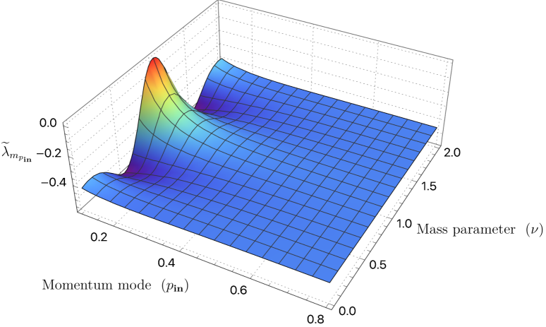
Refer to caption
(a) For fp𝐢𝐧=0subscript𝑓subscript𝑝𝐢𝐧0f_{p_{\bf in}}=0.
Refer to caption
(b) For small fp𝐢𝐧0subscript𝑓subscript𝑝𝐢𝐧0f_{p_{\bf in}}\neq 0.
Figure 6.2: Representative 3D plot of the eignenvalue of the partial transposed matrix with the mass parameter and the corresponding momentum mode associated with the computation. Here the partial transpose operation is taken with respect to the quantum vacuum state of the first Bunch Davies state which is characterizing the corresponding open chart of the global de Sitter space.
Refer to caption
(a) For fp𝐢𝐧=0subscript𝑓subscript𝑝𝐢𝐧0f_{p_{\bf in}}=0.
Refer to caption
(b) For small fp𝐢𝐧0subscript𝑓subscript𝑝𝐢𝐧0f_{p_{\bf in}}\neq 0.
Figure 6.3: Graphical behaviour of the of the eignenvalue of the partial transposed matrix with the mass parameter for given value of the momentum mode associated with the computation.
Refer to caption
(a) For fp𝐢𝐧=0subscript𝑓subscript𝑝𝐢𝐧0f_{p_{\bf in}}=0.
Refer to caption
(b) For small fp𝐢𝐧0subscript𝑓subscript𝑝𝐢𝐧0f_{p_{\bf in}}\neq 0.
Figure 6.4: Graphical behaviour of the of the eignenvalue of the partial transposed matrix with the momentum mode associated with the computation for the given value of mass parameter.
Refer to caption
(a) For fp𝐢𝐧=0subscript𝑓subscript𝑝𝐢𝐧0f_{p_{\bf in}}=0.
Refer to caption
(b) For small fp𝐢𝐧0subscript𝑓subscript𝑝𝐢𝐧0f_{p_{\bf in}}\neq 0.
Figure 6.5: Graphical behaviour of the of the logarithmic negativity computed from the negative eigenvalues of the partial transposed reduced density matrix with the mass parameter associated with the computation for the given value of momentum mode.
Refer to caption
(a) For fp𝐢𝐧=0subscript𝑓subscript𝑝𝐢𝐧0f_{p_{\bf in}}=0.
Refer to caption
(b) For small fp𝐢𝐧0subscript𝑓subscript𝑝𝐢𝐧0f_{p_{\bf in}}\neq 0.
Figure 6.6: Graphical behaviour of the of the logarithmic negativity computed from the negative eigenvalues of the partial transposed reduced density matrix with the momentum mode associated with the computation for the given value of mass parameter.

In figure (6.2(a)) and (6.2(b)), we have depicted the representative 3D plot of the eignenvalue of the partial transposed matrix with the mass parameter and the corresponding momentum mode associated with the computation. In these plots we have considered two possibilities, vanishing fp𝐢𝐧=0subscript𝑓subscript𝑝𝐢𝐧0f_{p_{\bf in}}=0 and a very small value but fp𝐢𝐧0subscript𝑓subscript𝑝𝐢𝐧0f_{p_{\bf in}}\neq 0. Here the partial transpose operation is taken with respect to the quantum vacuum state of the first Bunch Davies state which is characterizing the corresponding open chart of the global de Sitter space. The outcomes and the physical interpretation of these plots are very interesting which we are writing point-wise in the following:

  1. 1.

    In these plots we can clearly observe that the corresponding eignevalue that we have plotted for the mode having m𝐩𝐢𝐧=0subscript𝑚subscript𝐩𝐢𝐧0m_{\bf p_{in}}=0 gives negative contributions for both figure (6.2(a)) and (6.2(b)). This is a clear signature of having quantum mechanical entanglement in the biverse as well as well as the multiverse picture that we have theoretically constructed in this paper.

  2. 2.

    The other higher modes m𝐩𝐢𝐧>0subscript𝑚subscript𝐩𝐢𝐧0m_{\bf p_{in}}>0 gives positive contribution to the eigenvalue for which we have not incorporated those plots in this paper. Most importantly such contributions will not be in support of quantum entanglement in the present theoretical picture, so those solutions are not interesting in the present context.

  3. 3.

    Comparing both of these plots we can also observe that for fp𝐢𝐧=0subscript𝑓subscript𝑝𝐢𝐧0f_{p_{\bf in}}=0 we get less quantum entanglement compared to the case that we have studied for small fp𝐢𝐧0subscript𝑓subscript𝑝𝐢𝐧0f_{p_{\bf in}}\neq 0.

  4. 4.

    Also we have found that for heavy mass field which is governed by ν=i|ν|𝜈𝑖𝜈\nu=-i|\nu| or ν2<0superscript𝜈20\nu^{2}<0 the corresponding eigenvalue of the partial transposed version of the reduced density matrix is highly positive. Since this fact is not the desirable one, we have not included such plots in this paper. But it is strictly confirmed that to get high amount of entanglement heavy field is not desirable in the present prescribed framework. For this reason we have only shown the plots for massless or partially massless fields which can be studied using the solution for the branch ν>0𝜈0\nu>0.

  5. 5.

    From both of these plots we can clearly observe that for the values of the mass parameter ν=1/2𝜈12\nu=1/2 (conformal coupling) and ν=3/2𝜈32\nu=3/2 (massless case) there are two dips in the eigenvalue spectrum, which correspond to maximum entanglement from the theoretical set up under consideration. On the other hand, in both of these plots we see that at ν=1𝜈1\nu=1 there is minimum contribution from the quantum entanglement compared to the previously mentioned two values of the mass parameter ν𝜈\nu.

  6. 6.

    For any other values of the mass parameter lying within the window 0<ν<20𝜈20<\nu<2 we get the intermediate amount of quantum mechanical entanglement. Particularly, it is important to note that for ν=0𝜈0\nu=0 the amount of entanglement is larger than the amount of entanglement obtained for the value ν=2𝜈2\nu=2.

  7. 7.

    It seems like that the eigenvalue spectrum is distributed symmetrically around the value of the mass parameter ν=1𝜈1\nu=1. But actually this is not the case. Crucial observation suggests that the hight of the spectrum is lesser at ν=0𝜈0\nu=0 compared to ν=2𝜈2\nu=2.

  8. 8.

    In both of these plots we have restricted our parameter space within the region 0<p𝐢𝐧<0.80subscript𝑝𝐢𝐧0.80<p_{\bf in}<0.8 and 0<ν<20𝜈20<\nu<2, which we found the most suitable parameter space to get the negative contribution from the eigenvalue spectrum for the mode m𝐩𝐢𝐧=0subscript𝑚subscript𝐩𝐢𝐧0m_{\bf p_{in}}=0.

In figure (6.3(a)) and (6.3(b)), we have depicted the representative graphical behaviour of the of the eignenvalue of the partial transposed matrix with the mass parameter for given value of the momentum mode associated with the computation. In these plots we have considered two possibilities, vanishing fp𝐢𝐧=0subscript𝑓subscript𝑝𝐢𝐧0f_{p_{\bf in}}=0 and a very small value but fp𝐢𝐧0subscript𝑓subscript𝑝𝐢𝐧0f_{p_{\bf in}}\neq 0. In both of these plots we have fixed the value of the momentum mode within the region 0.2<p𝐢𝐧<0.50.2subscript𝑝𝐢𝐧0.50.2<p_{\bf in}<0.5 and have studied the behaviour of the eigenvalue spectrum with respect to mass parameter within the range 0<ν<20𝜈20<\nu<2. In our computation we found that this is the most desirable window of parameters within which one can get maximum contribution from the quantum entanglement in terms of getting maximum negative contribution from the eigenvalue.

Further, in figure (6.4(a)) and (6.4(b)), we have depicted the representative graphical graphical behaviour of the of the eignenvalue of the partial transposed matrix with the momentum mode associated with the computation for the given value of mass parameter. In these plots we have considered two possibilities, vanishing fp𝐢𝐧=0subscript𝑓subscript𝑝𝐢𝐧0f_{p_{\bf in}}=0 and a very small value but fp𝐢𝐧0subscript𝑓subscript𝑝𝐢𝐧0f_{p_{\bf in}}\neq 0. In both of these plots we have fixed the value of the mass parameter within the region 1<ν<7/41𝜈741<\nu<7/4 and have studied the behaviour of the eigenvalue spectrum with respect to momentum mode within the range 0.1<p𝐢𝐧<0.80.1subscript𝑝𝐢𝐧0.80.1<p_{\bf in}<0.8. We have found that for very small value of momentum mode with the mass parameter in the region ν<1𝜈1\nu<1 is not desirable in the present context as it gives very large positive eigenvalue. Also from this analysis we have found that for very large value of the momentum mode for any values of the mass parameter ν𝜈\nu the corresponding eigenvalue spectrum will saturate to a negative value. After comparing figure (6.4(a)) and (6.4(b)), we also have found that this asymptotic saturation value for small fp𝐢𝐧0subscript𝑓subscript𝑝𝐢𝐧0f_{p_{\bf in}}\neq 0 is larger compared to result obtained from fp𝐢𝐧=0subscript𝑓subscript𝑝𝐢𝐧0f_{p_{\bf in}}=0 case.

Next, in figure (6.5(a)) and (6.5(b)), we have depicted the representative graphical graphical behaviour of the the logarithmic negativity computed from the negative eigenvalues of the partial transposed reduced density matrix with the mass parameter associated with the computation for the given value of momentum mode. Finally, in figure (6.6(a)) and (6.6(b)), we have depicted the representative graphical graphical behaviour of the the logarithmic negativity with the momentum mode for the given value of mass parameter. In these plots we have considered two possibilities, vanishing fp𝐢𝐧=0subscript𝑓subscript𝑝𝐢𝐧0f_{p_{\bf in}}=0 and a very small value but fp𝐢𝐧0subscript𝑓subscript𝑝𝐢𝐧0f_{p_{\bf in}}\neq 0. The outcomes and the physical interpretation of these plots are very interesting which we are writing point-wise in the following:

  1. 1.

    From the figure (6.5(a)) and (6.5(b)), we have found that for fp𝐢𝐧=0subscript𝑓subscript𝑝𝐢𝐧0f_{p_{\bf in}}=0 logarithmic negativity vanishes at ν=1𝜈1\nu=1, but for small fp𝐢𝐧0subscript𝑓subscript𝑝𝐢𝐧0f_{p_{\bf in}}\neq 0 it is non zero but very small. It further implies that at the value of the mass parameter ν=1𝜈1\nu=1 we have almost negligible contribution from the quantum mechanical entanglement on large scales. Additionally it is important to note that, this particular outcome is obtained for a specific value of the momentum mode, p𝐢𝐧=0.2subscript𝑝𝐢𝐧0.2p_{\bf in}=0.2.

  2. 2.

    On the other hand, we have found that at ν=1/2𝜈12\nu=1/2 and ν=3/2𝜈32\nu=3/2 the obtained value of the logarithmic negativity from the present theoretical set up reach the maximum value, which further correspond to the maximum quantum mechanical entanglement or maximum correlation. This outcome is true for the momentum mode, p𝐢𝐧=0.2subscript𝑝𝐢𝐧0.2p_{\bf in}=0.2. One important thing here to mention that the large scale limit corresponds to the small value of the momentum mode p𝐢𝐧subscript𝑝𝐢𝐧p_{\bf in} in our present computation.

  3. 3.

    For the other values of momentum mode lying within the window 0.2<p𝐢𝐧<0.50.2subscript𝑝𝐢𝐧0.50.2<p_{\bf in}<0.5 we have found that the variation with respect to the mass parameter ν𝜈\nu is less compared to the case that we have studied for the momentum mode p𝐢𝐧=0.2subscript𝑝𝐢𝐧0.2p_{\bf in}=0.2. Comparing all the outcomes obtained for the different momentum modes within the mentioned range we have found that if we increase the value of p𝐢𝐧subscript𝑝𝐢𝐧p_{\bf in} then the corresponding variation is reduced and we get intermediate values of negativity, which corresponds to the intermediate amount of quantum mechanical entanglement for the system under consideration. This further implies the fact that lower values of the momentum mode for the prescribed analysis is more desirable as it is giving higher amplitude of logarithmic negativity, hence higher amount of quantum mechanical entanglement.

  4. 4.

    We have also found that the underlying quantum mechanical entanglement directly put impact on the shape of the spectrum of logarithmic negativity at the large scales which nearly equals or exceeds the mass parameter’s value ν3/2similar-to𝜈32\nu\sim 3/2.

  5. 5.

    Further, in figure (6.6(a)) and (6.6(b)), we have found out that for large values of the momentum mode p𝐢𝐧>0.5subscript𝑝𝐢𝐧0.5p_{\bf in}>0.5 the corresponding logarithmic negativity computed from the prescribed theoretical set up saturates to a constant non zero positive non negligible value. This further implies constant amount of quantum entanglement for any arbitrary positive real value of the mass parameter ν𝜈\nu. However, in this asymptotic limit one cannot distinguish the individual effect of the mass parameter in the present computation. This also implies that the low momentum modes are more desirable for the present analysis to distinguish the individual effects of the mass parameter ν𝜈\nu.

  6. 6.

    Last but not least, we have also found that except ν=3/2𝜈32\nu=3/2 for all other values of the mass parameter ν𝜈\nu we get a sharp changing behaviour in the specific value of the momentum mode.

6.6 Small scale limit of logarithmic negativity: Analytical study

In the small scale limit one needs to take the limit p𝐢𝐧subscript𝑝𝐢𝐧p_{\bf in}\rightarrow\infty to compute the logarithmic negativity from the present computational set up. In this limit we have:

Δ1=Δ11,Δ2=Δ20,Δ3,s=Δ3,s1,Δ4,s=Δ4,s0.formulae-sequencesubscriptΔ1subscriptsuperscriptΔ11subscriptΔ2subscriptsuperscriptΔ20subscriptΔ3𝑠subscriptsuperscriptΔ3𝑠1subscriptΔ4𝑠subscriptsuperscriptΔ4𝑠0\displaystyle\Delta_{1}=\Delta^{*}_{1}\rightarrow 1,\quad\Delta_{2}=\Delta^{*}_{2}\rightarrow 0,\quad\Delta_{3,s}=\Delta^{*}_{3,s}\rightarrow 1,\quad\Delta_{4,s}=\Delta^{*}_{4,s}\rightarrow 0. (6.87)

The following simplified formulas in the small scale limit are obtained after taking partial transposition with regard to the subsystem corresponding to the first Bunch Davies quantum vacuum state:

ρm𝐩𝐢𝐧T,𝐁𝐃𝟏subscriptsuperscript𝜌𝑇subscript𝐁𝐃1subscript𝑚subscript𝐩𝐢𝐧\displaystyle\rho^{T,{\bf BD_{1}}}_{m_{\bf p_{in}}} =\displaystyle= (1|γp𝐢𝐧|2)2(1+fp𝐢𝐧)|γp𝐢𝐧|2m𝐩𝐢𝐧{|0𝐩𝐨𝐮𝐭𝐁𝐃𝟏|m𝐩𝐢𝐧𝐋𝐁𝐃𝟏0|m𝐩𝐢𝐧|𝐋\displaystyle\frac{\left(1-|\gamma_{p_{\bf in}}|^{2}\right)}{2\left(1+f_{p_{\bf in}}\right)}|\gamma_{p_{\bf in}}|^{2m_{\bf p_{in}}}\Bigg{\{}|0_{\bf p_{out}}\rangle_{\bf BD_{1}}|m_{\bf p_{in}}\rangle_{{\bf L}^{{}^{\prime}}}\leavevmode\nobreak\ {}_{\bf BD_{1}}\langle 0|{}_{{\bf L}^{{}^{\prime}}}\langle m_{\bf p_{in}}| (6.88)
+m𝐩𝐢𝐧+1|1𝐩𝐨𝐮𝐭𝐁𝐃𝟏|m𝐩𝐢𝐧𝐋𝐁𝐃𝟏0|m𝐩𝐢𝐧+1|𝐋\displaystyle+\sqrt{m_{\bf p_{in}}+1}|1_{\bf p_{out}}\rangle_{\bf BD_{1}}|m_{\bf p_{in}}\rangle_{{\bf L}^{{}^{\prime}}}\leavevmode\nobreak\ {}_{\bf BD_{1}}\langle 0|{}_{{\bf L}^{{}^{\prime}}}\langle m_{\bf p_{in}}+1|
+m𝐩𝐢𝐧+1|0𝐩𝐨𝐮𝐭𝐁𝐃𝟏|m𝐩𝐢𝐧+1𝐋𝐁𝐃𝟏1|m𝐩𝐢𝐧|𝐋\displaystyle+\sqrt{m_{\bf p_{in}}+1}|0_{\bf p_{out}}\rangle_{\bf BD_{1}}|m_{\bf p_{in}}+1\rangle_{{\bf L}^{{}^{\prime}}}\leavevmode\nobreak\ {}_{\bf BD_{1}}\langle 1|{}_{{\bf L}^{{}^{\prime}}}\langle m_{\bf p_{in}}|
+(m𝐩𝐢𝐧+1)|1𝐩𝐨𝐮𝐭𝐁𝐃𝟏|m𝐩𝐢𝐧+1𝐋𝐁𝐃𝟏1|m𝐩𝐢𝐧+1|}𝐋,\displaystyle+(m_{\bf p_{in}}+1)|1_{\bf p_{out}}\rangle_{\bf BD_{1}}|m_{\bf p_{in}}+1\rangle_{{\bf L}^{{}^{\prime}}}\leavevmode\nobreak\ {}_{\bf BD_{1}}\langle 1|{}_{{\bf L}^{{}^{\prime}}}\langle m_{\bf p_{in}}+1|\Bigg{\}},

and

ρm𝐩𝐢𝐧,sT,𝐁𝐃𝟏subscriptsuperscript𝜌𝑇subscript𝐁𝐃1subscript𝑚subscript𝐩𝐢𝐧𝑠\displaystyle\rho^{T,{\bf BD_{1}}}_{m_{\bf p_{in}},s} =\displaystyle= fp𝐢𝐧22(1+fp𝐢𝐧)|Γp𝐢𝐧,s|2m𝐩𝐢𝐧{|0𝐩𝐨𝐮𝐭𝐁𝐃𝟏|s,m𝐩𝐢𝐧𝐋𝐁𝐃𝟏0|s,m𝐩𝐢𝐧|𝐋\displaystyle\frac{f^{2}_{p_{\bf in}}}{2\left(1+f_{p_{\bf in}}\right)}|\Gamma_{{p_{\bf in}},s}|^{2m_{\bf p_{in}}}\Bigg{\{}|0_{\bf p_{out}}\rangle_{\bf BD_{1}}|s,m_{\bf p_{in}}\rangle_{{\bf L}^{{}^{\prime}}}\leavevmode\nobreak\ {}_{\bf BD_{1}}\langle 0|{}_{{\bf L}^{{}^{\prime}}}\langle s,m_{\bf p_{in}}| (6.89)
+m𝐩𝐢𝐧+1|1𝐩𝐨𝐮𝐭𝐁𝐃𝟏|s,m𝐩𝐢𝐧𝐋𝐁𝐃𝟏0|s,(m𝐩𝐢𝐧+1)|𝐋\displaystyle+\sqrt{m_{\bf p_{in}}+1}|1_{\bf p_{out}}\rangle_{\bf BD_{1}}|s,m_{\bf p_{in}}\rangle_{{\bf L}^{{}^{\prime}}}\leavevmode\nobreak\ {}_{\bf BD_{1}}\langle 0|{}_{{\bf L}^{{}^{\prime}}}\langle s,(m_{\bf p_{in}}+1)|
+m𝐩𝐢𝐧+1|0𝐩𝐨𝐮𝐭𝐁𝐃𝟏|s,m𝐩𝐢𝐧+1𝐋𝐁𝐃𝟏1|s,m𝐩𝐢𝐧|𝐋\displaystyle+\sqrt{m_{\bf p_{in}}+1}|0_{\bf p_{out}}\rangle_{\bf BD_{1}}|s,m_{\bf p_{in}}+1\rangle_{{\bf L}^{{}^{\prime}}}\leavevmode\nobreak\ {}_{\bf BD_{1}}\langle 1|{}_{{\bf L}^{{}^{\prime}}}\langle s,m_{\bf p_{in}}|
+(m𝐩𝐢𝐧+1)|1𝐩𝐨𝐮𝐭𝐁𝐃𝟏|s,(m𝐩𝐢𝐧+1)𝐋𝐁𝐃𝟏1|s,(m𝐩𝐢𝐧+1)|}𝐋.\displaystyle+(m_{\bf p_{in}}+1)|1_{\bf p_{out}}\rangle_{\bf BD_{1}}|s,(m_{\bf p_{in}}+1)\rangle_{{\bf L}^{{}^{\prime}}}\leavevmode\nobreak\ {}_{\bf BD_{1}}\langle 1|{}_{{\bf L}^{{}^{\prime}}}\langle s,(m_{\bf p_{in}}+1)|\Bigg{\}}.

Let us express the above mentioned transposed version of the reduced density matrices computed from the complementary and particular integral part in square matrix form, which are given by the following expressions:

ρm𝐩𝐢𝐧T,𝐁𝐃𝟏subscriptsuperscript𝜌𝑇subscript𝐁𝐃1subscript𝑚subscript𝐩𝐢𝐧\displaystyle\rho^{T,{\bf BD_{1}}}_{m_{\bf p_{in}}} =\displaystyle= (1|γp𝐢𝐧|2)2(1+fp𝐢𝐧)|γp𝐢𝐧|2m𝐩𝐢𝐧(1m𝐩𝐢𝐧+1 0m𝐩𝐢𝐧+1(m𝐩𝐢𝐧+1) 00 0 0),1superscriptsubscript𝛾subscript𝑝𝐢𝐧221subscript𝑓subscript𝑝𝐢𝐧superscriptsubscript𝛾subscript𝑝𝐢𝐧2subscript𝑚subscript𝐩𝐢𝐧1subscript𝑚subscript𝐩𝐢𝐧1 0subscript𝑚subscript𝐩𝐢𝐧1subscript𝑚subscript𝐩𝐢𝐧1 00 0 0\displaystyle\frac{\left(1-|\gamma_{p_{\bf in}}|^{2}\right)}{2\left(1+f_{p_{\bf in}}\right)}|\gamma_{p_{\bf in}}|^{2m_{\bf p_{in}}}\left(\begin{array}[]{ccc}1&\leavevmode\nobreak\ \leavevmode\nobreak\ \leavevmode\nobreak\ \sqrt{m_{\bf p_{in}}+1}&\leavevmode\nobreak\ \leavevmode\nobreak\ \leavevmode\nobreak\ 0\\ \sqrt{m_{\bf p_{in}}+1}&\leavevmode\nobreak\ \leavevmode\nobreak\ \leavevmode\nobreak\ (m_{\bf p_{in}}+1)&\leavevmode\nobreak\ \leavevmode\nobreak\ \leavevmode\nobreak\ 0\\ 0&\leavevmode\nobreak\ \leavevmode\nobreak\ \leavevmode\nobreak\ 0&\leavevmode\nobreak\ \leavevmode\nobreak\ \leavevmode\nobreak\ 0\end{array}\right), (6.93)
ρm𝐩𝐢𝐧,sT,𝐁𝐃𝟏subscriptsuperscript𝜌𝑇subscript𝐁𝐃1subscript𝑚subscript𝐩𝐢𝐧𝑠\displaystyle\rho^{T,{\bf BD_{1}}}_{m_{\bf p_{in}},s} =\displaystyle= fp𝐢𝐧22(1+fp𝐢𝐧)|Γp𝐢𝐧,s|2m𝐩𝐢𝐧(1m𝐩𝐢𝐧+1 0m𝐩𝐢𝐧+1(m𝐩𝐢𝐧+1) 00 0 0),subscriptsuperscript𝑓2subscript𝑝𝐢𝐧21subscript𝑓subscript𝑝𝐢𝐧superscriptsubscriptΓsubscript𝑝𝐢𝐧𝑠2subscript𝑚subscript𝐩𝐢𝐧1subscript𝑚subscript𝐩𝐢𝐧1 0subscript𝑚subscript𝐩𝐢𝐧1subscript𝑚subscript𝐩𝐢𝐧1 00 0 0\displaystyle\frac{f^{2}_{p_{\bf in}}}{2\left(1+f_{p_{\bf in}}\right)}|\Gamma_{{p_{\bf in}},s}|^{2m_{\bf p_{in}}}\left(\begin{array}[]{ccc}1&\leavevmode\nobreak\ \leavevmode\nobreak\ \leavevmode\nobreak\ \sqrt{m_{\bf p_{in}}+1}&\leavevmode\nobreak\ \leavevmode\nobreak\ \leavevmode\nobreak\ 0\\ \sqrt{m_{\bf p_{in}}+1}&\leavevmode\nobreak\ \leavevmode\nobreak\ \leavevmode\nobreak\ (m_{\bf p_{in}}+1)&\leavevmode\nobreak\ \leavevmode\nobreak\ \leavevmode\nobreak\ 0\\ 0&\leavevmode\nobreak\ \leavevmode\nobreak\ \leavevmode\nobreak\ 0&\leavevmode\nobreak\ \leavevmode\nobreak\ \leavevmode\nobreak\ 0\end{array}\right), (6.97)

Next we compute the eigenvalue equation from the total partial transposed matrix after summing over source mode s𝑠s, which is given by the following expression:

λ~m𝐩𝐢𝐧2(λ~m𝐩𝐢𝐧(1|γp𝐢𝐧|2)2(1+fp𝐢𝐧)|γp𝐢𝐧|2m𝐩𝐢𝐧(m𝐩𝐢𝐧+2)fp𝐢𝐧22(1+fp𝐢𝐧)(m𝐩𝐢𝐧+2)gp𝐢𝐧)=0.subscriptsuperscript~𝜆2subscript𝑚subscript𝐩𝐢𝐧subscript~𝜆subscript𝑚subscript𝐩𝐢𝐧1superscriptsubscript𝛾subscript𝑝𝐢𝐧221subscript𝑓subscript𝑝𝐢𝐧superscriptsubscript𝛾subscript𝑝𝐢𝐧2subscript𝑚subscript𝐩𝐢𝐧subscript𝑚subscript𝐩𝐢𝐧2subscriptsuperscript𝑓2subscript𝑝𝐢𝐧21subscript𝑓subscript𝑝𝐢𝐧subscript𝑚subscript𝐩𝐢𝐧2subscript𝑔subscript𝑝𝐢𝐧0\displaystyle\widetilde{\lambda}^{2}_{m_{\bf p_{in}}}\left(\widetilde{\lambda}_{m_{\bf p_{in}}}-\frac{\left(1-|\gamma_{p_{\bf in}}|^{2}\right)}{2\left(1+f_{p_{\bf in}}\right)}|\gamma_{p_{\bf in}}|^{2m_{\bf p_{in}}}(m_{\bf p_{in}}+2)-\frac{f^{2}_{p_{\bf in}}}{2\left(1+f_{p_{\bf in}}\right)}(m_{\bf p_{in}}+2)g_{p_{\bf in}}\right)=0.\quad\quad\quad (6.98)

The non trivial root of the eigenvalue computed from the (m𝐩𝐢𝐧,m𝐩𝐢𝐧+1)subscript𝑚subscript𝐩𝐢𝐧subscript𝑚subscript𝐩𝐢𝐧1(m_{\bf p_{in}},m_{\bf p_{in}}+1) block in the small scale limit is given by:

λ~m𝐩𝐢𝐧subscript~𝜆subscript𝑚subscript𝐩𝐢𝐧\displaystyle\widetilde{\lambda}_{m_{\bf p_{in}}} =\displaystyle= (m𝐩𝐢𝐧+2)2(1+fp𝐢𝐧)[(1|γp𝐢𝐧|2)|γp𝐢𝐧|2m𝐩𝐢𝐧+fp𝐢𝐧2gp𝐢𝐧],subscript𝑚subscript𝐩𝐢𝐧221subscript𝑓subscript𝑝𝐢𝐧delimited-[]1superscriptsubscript𝛾subscript𝑝𝐢𝐧2superscriptsubscript𝛾subscript𝑝𝐢𝐧2subscript𝑚subscript𝐩𝐢𝐧subscriptsuperscript𝑓2subscript𝑝𝐢𝐧subscript𝑔subscript𝑝𝐢𝐧\displaystyle\frac{(m_{\bf p_{in}}+2)}{2\left(1+f_{p_{\bf in}}\right)}\Bigg{[}\left(1-|\gamma_{p_{\bf in}}|^{2}\right)|\gamma_{p_{\bf in}}|^{2m_{\bf p_{in}}}+f^{2}_{p_{\bf in}}g_{p_{\bf in}}\Bigg{]}, (6.99)

where we define:

gp𝐢𝐧:=s=0|Γp𝐢𝐧,s|2m𝐩𝐢𝐧.assignsubscript𝑔subscript𝑝𝐢𝐧subscriptsuperscript𝑠0superscriptsubscriptΓsubscript𝑝𝐢𝐧𝑠2subscript𝑚subscript𝐩𝐢𝐧\displaystyle g_{p_{\bf in}}:=\sum^{\infty}_{s=0}|\Gamma_{{p_{\bf in}},s}|^{2m_{\bf p_{in}}}. (6.100)

Then the logarithmic negativity from the present set up can be further computed as:

𝒩𝒩\displaystyle{\cal LN} =\displaystyle= ln(2λ~m𝐩𝐢𝐧<0λ~m𝐩𝐢𝐧+1)2subscriptsubscript~𝜆subscript𝑚subscript𝐩𝐢𝐧0subscript~𝜆subscript𝑚subscript𝐩𝐢𝐧1\displaystyle\ln\left(2\sum_{\widetilde{\lambda}_{m_{\bf p_{in}}}<0}\widetilde{\lambda}_{m_{\bf p_{in}}}+1\right) (6.101)
=\displaystyle= ln((m𝐩𝐢𝐧+2)(1+fp𝐢𝐧)[(1|γp𝐢𝐧|2)|γp𝐢𝐧|2m𝐩𝐢𝐧+fp𝐢𝐧2gp𝐢𝐧]+1).subscript𝑚subscript𝐩𝐢𝐧21subscript𝑓subscript𝑝𝐢𝐧delimited-[]1superscriptsubscript𝛾subscript𝑝𝐢𝐧2superscriptsubscript𝛾subscript𝑝𝐢𝐧2subscript𝑚subscript𝐩𝐢𝐧subscriptsuperscript𝑓2subscript𝑝𝐢𝐧subscript𝑔subscript𝑝𝐢𝐧1\displaystyle\ln\Bigg{(}\frac{(m_{\bf p_{in}}+2)}{\left(1+f_{p_{\bf in}}\right)}\Bigg{[}\left(1-|\gamma_{p_{\bf in}}|^{2}\right)|\gamma_{p_{\bf in}}|^{2m_{\bf p_{in}}}+f^{2}_{p_{\bf in}}g_{p_{\bf in}}\Bigg{]}+1\Bigg{)}.

We get a negative contribution from the eigenvalue if the following condition is satisfied for the small scale limiting situation:

[|γp𝐢𝐧|2m𝐩𝐢𝐧(1|γp𝐢𝐧|2)+fp𝐢𝐧2gp𝐢𝐧]<0.delimited-[]superscriptsubscript𝛾subscript𝑝𝐢𝐧2subscript𝑚subscript𝐩𝐢𝐧1superscriptsubscript𝛾subscript𝑝𝐢𝐧2subscriptsuperscript𝑓2subscript𝑝𝐢𝐧subscript𝑔subscript𝑝𝐢𝐧0\displaystyle\Bigg{[}|\gamma_{p_{\bf in}}|^{2m_{\bf p_{in}}}\left(1-|\gamma_{p_{\bf in}}|^{2}\right)+f^{2}_{p_{\bf in}}g_{p_{\bf in}}\Bigg{]}<0. (6.102)

Now from the previous analysis we have already found that m𝐩𝐢𝐧=0subscript𝑚subscript𝐩𝐢𝐧0m_{\bf p_{in}}=0 mode is most desirable one to obtain the negative contribution from the eigenvalue spectrum. In such a case using the well known Riemann zeta function regularization we can write the following result for m𝐩𝐢𝐧=0subscript𝑚subscript𝐩𝐢𝐧0m_{\bf p_{in}}=0:

gp𝐢𝐧:=s=01=1+s=11=1+(1+1+1+)=1+ζ(0)=112=12.assignsubscript𝑔subscript𝑝𝐢𝐧subscriptsuperscript𝑠011subscriptsuperscript𝑠1111111𝜁011212\displaystyle g_{p_{\bf in}}:=\sum^{\infty}_{s=0}1=1+\sum^{\infty}_{s=1}1=1+\left(1+1+1+\cdots\right)=1+\zeta(0)=1-\frac{1}{2}=\frac{1}{2}. (6.103)

which also suggests the following restriction on the small scale limiting circumstance:

|γp𝐢𝐧|>(1+fp𝐢𝐧22).subscript𝛾subscript𝑝𝐢𝐧1subscriptsuperscript𝑓2subscript𝑝𝐢𝐧2\displaystyle|\gamma_{p_{\bf in}}|>\sqrt{\Bigg{(}1+\frac{f^{2}_{p_{\bf in}}}{2}\Bigg{)}}. (6.104)

6.7 Massless limit of logarithmic negativity: Analytical study

In the massless limit one needs to take the limit ν=3/2𝜈32\nu=3/2 (exact masslessness) or ν=1/2𝜈12\nu=1/2 (conformal invariance) to compute the logarithmic negativity from the present computational set up. In this limit we have:

Δ1(A~D~γp𝐢𝐧)u,Δ20,Δ3,s(A~nD~nΓp𝐢𝐧,n)Un,Δ4,s0.formulae-sequencesubscriptΔ1~𝐴~𝐷subscript𝛾subscript𝑝𝐢𝐧𝑢formulae-sequencesubscriptΔ20formulae-sequencesubscriptΔ3𝑠subscript~𝐴𝑛subscript~𝐷𝑛subscriptΓsubscript𝑝𝐢𝐧𝑛subscript𝑈𝑛subscriptΔ4𝑠0\displaystyle\Delta_{1}\rightarrow\bigg{(}\widetilde{A}-\widetilde{D}\gamma_{p_{\bf in}}\bigg{)}u,\quad\Delta_{2}\rightarrow 0,\quad\Delta_{3,s}\rightarrow\bigg{(}\widetilde{A}_{n}-\widetilde{D}_{n}\Gamma_{{p_{\bf in}},n}\bigg{)}U_{n},\quad\Delta_{4,s}\rightarrow 0.\quad\quad\quad (6.105)

The partial transposition operation for the subsystem corresponding to the first Bunch Davies quantum vacuum state is given by the following formulas for the massless limiting situation:

ρm𝐩𝐢𝐧T,𝐁𝐃𝟏subscriptsuperscript𝜌𝑇subscript𝐁𝐃1subscript𝑚subscript𝐩𝐢𝐧\displaystyle\rho^{T,{\bf BD_{1}}}_{m_{\bf p_{in}}} =\displaystyle= (1|γp𝐢𝐧|2)2(1+fp𝐢𝐧)|γp𝐢𝐧|2m𝐩𝐢𝐧{|0𝐩𝐨𝐮𝐭𝐁𝐃𝟏|m𝐩𝐢𝐧𝐋𝐁𝐃𝟏0|m𝐩𝐢𝐧|𝐋\displaystyle\frac{\left(1-|\gamma_{p_{\bf in}}|^{2}\right)}{2\left(1+f_{p_{\bf in}}\right)}|\gamma_{p_{\bf in}}|^{2m_{\bf p_{in}}}\Bigg{\{}|0_{\bf p_{out}}\rangle_{\bf BD_{1}}|m_{\bf p_{in}}\rangle_{{\bf L}^{{}^{\prime}}}\leavevmode\nobreak\ {}_{\bf BD_{1}}\langle 0|{}_{{\bf L}^{{}^{\prime}}}\langle m_{\bf p_{in}}| (6.106)
+Δ1m𝐩𝐢𝐧+1|1𝐩𝐨𝐮𝐭𝐁𝐃𝟏|m𝐩𝐢𝐧𝐋𝐁𝐃𝟏0|m𝐩𝐢𝐧+1|𝐋\displaystyle+\Delta^{*}_{1}\sqrt{m_{\bf p_{in}}+1}|1_{\bf p_{out}}\rangle_{\bf BD_{1}}|m_{\bf p_{in}}\rangle_{{\bf L}^{{}^{\prime}}}\leavevmode\nobreak\ {}_{\bf BD_{1}}\langle 0|{}_{{\bf L}^{{}^{\prime}}}\langle m_{\bf p_{in}}+1|
+Δ1m𝐩𝐢𝐧+1|0𝐩𝐨𝐮𝐭𝐁𝐃𝟏|m𝐩𝐢𝐧+1𝐋𝐁𝐃𝟏1|m𝐩𝐢𝐧|𝐋\displaystyle+\Delta_{1}\sqrt{m_{\bf p_{in}}+1}|0_{\bf p_{out}}\rangle_{\bf BD_{1}}|m_{\bf p_{in}}+1\rangle_{{\bf L}^{{}^{\prime}}}\leavevmode\nobreak\ {}_{\bf BD_{1}}\langle 1|{}_{{\bf L}^{{}^{\prime}}}\langle m_{\bf p_{in}}|
+|Δ1|2(m𝐩𝐢𝐧+1)|1𝐩𝐨𝐮𝐭𝐁𝐃𝟏|m𝐩𝐢𝐧+1𝐋𝐁𝐃𝟏1|m𝐩𝐢𝐧+1|}𝐋,\displaystyle+|\Delta_{1}|^{2}(m_{\bf p_{in}}+1)|1_{\bf p_{out}}\rangle_{\bf BD_{1}}|m_{\bf p_{in}}+1\rangle_{{\bf L}^{{}^{\prime}}}\leavevmode\nobreak\ {}_{\bf BD_{1}}\langle 1|{}_{{\bf L}^{{}^{\prime}}}\langle m_{\bf p_{in}}+1|\Bigg{\}},

and

ρm𝐩𝐢𝐧,sT,𝐁𝐃𝟏subscriptsuperscript𝜌𝑇subscript𝐁𝐃1subscript𝑚subscript𝐩𝐢𝐧𝑠\displaystyle\rho^{T,{\bf BD_{1}}}_{m_{\bf p_{in}},s} =\displaystyle= fp𝐢𝐧22(1+fp𝐢𝐧)|Γp𝐢𝐧,s|2m𝐩𝐢𝐧{|0𝐩𝐨𝐮𝐭𝐁𝐃𝟏|s,m𝐩𝐢𝐧𝐋𝐁𝐃𝟏0|s,m𝐩𝐢𝐧|𝐋\displaystyle\frac{f^{2}_{p_{\bf in}}}{2\left(1+f_{p_{\bf in}}\right)}|\Gamma_{{p_{\bf in}},s}|^{2m_{\bf p_{in}}}\Bigg{\{}|0_{\bf p_{out}}\rangle_{\bf BD_{1}}|s,m_{\bf p_{in}}\rangle_{{\bf L}^{{}^{\prime}}}\leavevmode\nobreak\ {}_{\bf BD_{1}}\langle 0|{}_{{\bf L}^{{}^{\prime}}}\langle s,m_{\bf p_{in}}| (6.107)
+Δ3,sm𝐩𝐢𝐧+1|1𝐩𝐨𝐮𝐭𝐁𝐃𝟏|s,m𝐩𝐢𝐧𝐋𝐁𝐃𝟏0|s,(m𝐩𝐢𝐧+1)|𝐋\displaystyle+\Delta^{*}_{3,s}\sqrt{m_{\bf p_{in}}+1}|1_{\bf p_{out}}\rangle_{\bf BD_{1}}|s,m_{\bf p_{in}}\rangle_{{\bf L}^{{}^{\prime}}}\leavevmode\nobreak\ {}_{\bf BD_{1}}\langle 0|{}_{{\bf L}^{{}^{\prime}}}\langle s,(m_{\bf p_{in}}+1)|
+Δ3,sm𝐩𝐢𝐧+1|0𝐩𝐨𝐮𝐭𝐁𝐃𝟏|s,m𝐩𝐢𝐧+1𝐋𝐁𝐃𝟏1|s,m𝐩𝐢𝐧|𝐋\displaystyle+\Delta_{3,s}\sqrt{m_{\bf p_{in}}+1}|0_{\bf p_{out}}\rangle_{\bf BD_{1}}|s,m_{\bf p_{in}}+1\rangle_{{\bf L}^{{}^{\prime}}}\leavevmode\nobreak\ {}_{\bf BD_{1}}\langle 1|{}_{{\bf L}^{{}^{\prime}}}\langle s,m_{\bf p_{in}}|
+|Δ3,s|2(m𝐩𝐢𝐧+1)|1𝐩𝐨𝐮𝐭𝐁𝐃𝟏|s,(m𝐩𝐢𝐧+1)𝐋𝐁𝐃𝟏1|s,(m𝐩𝐢𝐧+1)|}𝐋.\displaystyle+|\Delta_{3,s}|^{2}(m_{\bf p_{in}}+1)|1_{\bf p_{out}}\rangle_{\bf BD_{1}}|s,(m_{\bf p_{in}}+1)\rangle_{{\bf L}^{{}^{\prime}}}\leavevmode\nobreak\ {}_{\bf BD_{1}}\langle 1|{}_{{\bf L}^{{}^{\prime}}}\langle s,(m_{\bf p_{in}}+1)|\Bigg{\}}.\quad

In this special case the factors Δ1subscriptΔ1\Delta_{1} and Δ3,ssubscriptΔ3𝑠\Delta_{3,s} can be further simplified as:

Δ1subscriptΔ1\displaystyle\Delta_{1} =\displaystyle= (A~D~γp𝐢𝐧)u~𝐴~𝐷subscript𝛾subscript𝑝𝐢𝐧𝑢\displaystyle\bigg{(}\widetilde{A}-\widetilde{D}\gamma_{p_{\bf in}}\bigg{)}u (6.108)
=\displaystyle= 1sinhπp𝐢𝐧[exp(πp𝐢𝐧)iexp(πp𝐢𝐧)(1+p𝐢𝐧)(1p𝐢𝐧)Γ(ip𝐢𝐧)Γ(ip𝐢𝐧)],1𝜋subscript𝑝𝐢𝐧delimited-[]𝜋subscript𝑝𝐢𝐧𝑖𝜋subscript𝑝𝐢𝐧1subscript𝑝𝐢𝐧1subscript𝑝𝐢𝐧Γ𝑖subscript𝑝𝐢𝐧Γ𝑖subscript𝑝𝐢𝐧\displaystyle\frac{1}{\sinh\pi p_{\bf in}}\Bigg{[}\exp(\pi p_{\bf in})-i\exp(-\pi p_{\bf in})\frac{(1+p_{\bf in})}{(1-p_{\bf in})}\frac{\Gamma(ip_{\bf in})}{\Gamma(-ip_{\bf in})}\Bigg{]},
Δ3,ssubscriptΔ3𝑠\displaystyle\Delta_{3,s} =\displaystyle= (A~sD~sΓp𝐢𝐧,s)Ussubscript~𝐴𝑠subscript~𝐷𝑠subscriptΓsubscript𝑝𝐢𝐧𝑠subscript𝑈𝑠\displaystyle\bigg{(}\widetilde{A}_{s}-\widetilde{D}_{s}\Gamma_{p_{{\bf in},s}}\bigg{)}U_{s} (6.109)
=\displaystyle= 1sinhπp𝐢𝐧,s[exp(πp𝐢𝐧,s)iexp(πp𝐢𝐧,s)(1+p𝐢𝐧,s)(1p𝐢𝐧,s)Γ(ip𝐢𝐧,s)Γ(ip𝐢𝐧,s)].1𝜋subscript𝑝𝐢𝐧𝑠delimited-[]𝜋subscript𝑝𝐢𝐧𝑠𝑖𝜋subscript𝑝𝐢𝐧𝑠1subscript𝑝𝐢𝐧𝑠1subscript𝑝𝐢𝐧𝑠Γ𝑖subscript𝑝𝐢𝐧𝑠Γ𝑖subscript𝑝𝐢𝐧𝑠\displaystyle\frac{1}{\sinh\pi p_{{\bf in},s}}\Bigg{[}\exp(\pi p_{{\bf in},s})-i\exp(-\pi p_{{\bf in},s})\frac{(1+p_{{\bf in},s})}{(1-p_{{\bf in},s})}\frac{\Gamma(ip_{{\bf in},s})}{\Gamma(-ip_{{\bf in},s})}\Bigg{]}.

Let us express the above mentioned transposed version of the reduced density matrices computed from the complementary and particular integral part in square matrix form, which are given by the following expressions for the massless case:

ρm𝐩𝐢𝐧T,𝐁𝐃𝟏subscriptsuperscript𝜌𝑇subscript𝐁𝐃1subscript𝑚subscript𝐩𝐢𝐧\displaystyle\rho^{T,{\bf BD_{1}}}_{m_{\bf p_{in}}} =\displaystyle= (1|γp𝐢𝐧|2)2(1+fp𝐢𝐧)|γp𝐢𝐧|2m𝐩𝐢𝐧(1m𝐩𝐢𝐧+1Δ1 0m𝐩𝐢𝐧+1Δ1 0 00 0 0),1superscriptsubscript𝛾subscript𝑝𝐢𝐧221subscript𝑓subscript𝑝𝐢𝐧superscriptsubscript𝛾subscript𝑝𝐢𝐧2subscript𝑚subscript𝐩𝐢𝐧1subscript𝑚subscript𝐩𝐢𝐧1subscriptsuperscriptΔ1 0subscript𝑚subscript𝐩𝐢𝐧1subscriptΔ1 0 00 0 0\displaystyle\frac{\left(1-|\gamma_{p_{\bf in}}|^{2}\right)}{2\left(1+f_{p_{\bf in}}\right)}|\gamma_{p_{\bf in}}|^{2m_{\bf p_{in}}}\left(\begin{array}[]{ccc}1&\leavevmode\nobreak\ \leavevmode\nobreak\ \leavevmode\nobreak\ \sqrt{m_{\bf p_{in}}+1}\Delta^{*}_{1}&\leavevmode\nobreak\ \leavevmode\nobreak\ \leavevmode\nobreak\ 0\\ \sqrt{m_{\bf p_{in}}+1}\Delta_{1}&\leavevmode\nobreak\ \leavevmode\nobreak\ \leavevmode\nobreak\ 0&\leavevmode\nobreak\ \leavevmode\nobreak\ \leavevmode\nobreak\ 0\\ 0&\leavevmode\nobreak\ \leavevmode\nobreak\ \leavevmode\nobreak\ 0&\leavevmode\nobreak\ \leavevmode\nobreak\ \leavevmode\nobreak\ 0\end{array}\right), (6.113)
ρm𝐩𝐢𝐧,sT,𝐁𝐃𝟏subscriptsuperscript𝜌𝑇subscript𝐁𝐃1subscript𝑚subscript𝐩𝐢𝐧𝑠\displaystyle\rho^{T,{\bf BD_{1}}}_{m_{\bf p_{in}},s} =\displaystyle= fp𝐢𝐧22(1+fp𝐢𝐧)|Γp𝐢𝐧,s|2m𝐩𝐢𝐧(1m𝐩𝐢𝐧+1Δ3,s 0m𝐩𝐢𝐧+1Δ3,s 0 00 0 0).subscriptsuperscript𝑓2subscript𝑝𝐢𝐧21subscript𝑓subscript𝑝𝐢𝐧superscriptsubscriptΓsubscript𝑝𝐢𝐧𝑠2subscript𝑚subscript𝐩𝐢𝐧1subscript𝑚subscript𝐩𝐢𝐧1subscriptsuperscriptΔ3𝑠 0subscript𝑚subscript𝐩𝐢𝐧1subscriptΔ3𝑠 0 00 0 0\displaystyle\frac{f^{2}_{p_{\bf in}}}{2\left(1+f_{p_{\bf in}}\right)}|\Gamma_{{p_{\bf in}},s}|^{2m_{\bf p_{in}}}\left(\begin{array}[]{ccc}1&\leavevmode\nobreak\ \leavevmode\nobreak\ \leavevmode\nobreak\ \sqrt{m_{\bf p_{in}}+1}\Delta^{*}_{3,s}&\leavevmode\nobreak\ \leavevmode\nobreak\ \leavevmode\nobreak\ 0\\ \sqrt{m_{\bf p_{in}}+1}\Delta_{3,s}&\leavevmode\nobreak\ \leavevmode\nobreak\ \leavevmode\nobreak\ 0&\leavevmode\nobreak\ \leavevmode\nobreak\ \leavevmode\nobreak\ 0\\ 0&\leavevmode\nobreak\ \leavevmode\nobreak\ \leavevmode\nobreak\ 0&\leavevmode\nobreak\ \leavevmode\nobreak\ \leavevmode\nobreak\ 0\end{array}\right). (6.117)

Next we compute the eigenvalue equation from the total partial transposed matrix after summing over source mode s𝑠s, which is given by the following expression:

λ~m𝐩𝐢𝐧(λ~m𝐩𝐢𝐧2A¯m𝐩𝐢𝐧λ~m𝐩𝐢𝐧+B¯m𝐩𝐢𝐧)=0.subscript~𝜆subscript𝑚subscript𝐩𝐢𝐧subscriptsuperscript~𝜆2subscript𝑚subscript𝐩𝐢𝐧subscript¯𝐴subscript𝑚subscript𝐩𝐢𝐧subscript~𝜆subscript𝑚subscript𝐩𝐢𝐧subscript¯𝐵subscript𝑚subscript𝐩𝐢𝐧0\displaystyle\widetilde{\lambda}_{m_{\bf p_{in}}}\left(\widetilde{\lambda}^{2}_{m_{\bf p_{in}}}-\overline{A}_{m_{\bf p_{in}}}\widetilde{\lambda}_{m_{\bf p_{in}}}+\overline{B}_{m_{\bf p_{in}}}\right)=0. (6.118)

where in the above mentioned expression we have introduced some shorthand redefined symbols which are given by the following expressions:

A¯msubscript¯𝐴𝑚\displaystyle\overline{A}_{m} =\displaystyle= 12(1+fp𝐢𝐧)[(1|γp𝐢𝐧|2)|γp𝐢𝐧|2m+fp𝐢𝐧2gp𝐢𝐧],121subscript𝑓subscript𝑝𝐢𝐧delimited-[]1superscriptsubscript𝛾subscript𝑝𝐢𝐧2superscriptsubscript𝛾subscript𝑝𝐢𝐧2𝑚subscriptsuperscript𝑓2subscript𝑝𝐢𝐧subscript𝑔subscript𝑝𝐢𝐧\displaystyle\frac{1}{2\left(1+f_{p_{\bf in}}\right)}\Bigg{[}\left(1-|\gamma_{p_{\bf in}}|^{2}\right)|\gamma_{p_{\bf in}}|^{2m}+f^{2}_{p_{\bf in}}g_{p_{\bf in}}\Bigg{]},\quad (6.119)
B¯msubscript¯𝐵𝑚\displaystyle\overline{B}_{m} =\displaystyle= (m𝐩𝐢𝐧+1)4(1+fp𝐢𝐧)2[(1|γp𝐢𝐧|2)2|γp𝐢𝐧|4m|Δ1|2+fp𝐢𝐧4s=0|Γp𝐢𝐧,s|4m|Δ3,s|2].subscript𝑚subscript𝐩𝐢𝐧14superscript1subscript𝑓subscript𝑝𝐢𝐧2delimited-[]superscript1superscriptsubscript𝛾subscript𝑝𝐢𝐧22superscriptsubscript𝛾subscript𝑝𝐢𝐧4𝑚superscriptsubscriptΔ12subscriptsuperscript𝑓4subscript𝑝𝐢𝐧subscriptsuperscript𝑠0superscriptsubscriptΓsubscript𝑝𝐢𝐧𝑠4𝑚superscriptsubscriptΔ3𝑠2\displaystyle-\frac{\left(m_{\bf p_{in}}+1\right)}{4\left(1+f_{p_{\bf in}}\right)^{2}}\Bigg{[}\left(1-|\gamma_{p_{\bf in}}|^{2}\right)^{2}|\gamma_{p_{\bf in}}|^{4m}|\Delta_{1}|^{2}+f^{4}_{p_{\bf in}}\sum^{\infty}_{s=0}|\Gamma_{{p_{\bf in}},s}|^{4m}|\Delta_{3,s}|^{2}\Bigg{]}.\quad\quad (6.120)

The non trivial roots of the eigenvalue computed from the (m𝐩𝐢𝐧,m𝐩𝐢𝐧+1)subscript𝑚subscript𝐩𝐢𝐧subscript𝑚subscript𝐩𝐢𝐧1(m_{\bf p_{in}},m_{\bf p_{in}}+1) block are given by:

λ~m𝐩𝐢𝐧±subscriptsuperscript~𝜆plus-or-minussubscript𝑚subscript𝐩𝐢𝐧\displaystyle\widetilde{\lambda}^{\pm}_{m_{\bf p_{in}}} =\displaystyle= 12[A¯m𝐩𝐢𝐧±A¯m𝐩𝐢𝐧24B¯m𝐩𝐢𝐧].12delimited-[]plus-or-minussubscript¯𝐴subscript𝑚subscript𝐩𝐢𝐧subscriptsuperscript¯𝐴2subscript𝑚subscript𝐩𝐢𝐧4subscript¯𝐵subscript𝑚subscript𝐩𝐢𝐧\displaystyle\frac{1}{2}\Bigg{[}\overline{A}_{m_{\bf p_{in}}}\pm\sqrt{\overline{A}^{2}_{m_{\bf p_{in}}}-4\overline{B}_{m_{\bf p_{in}}}}\Bigg{]}. (6.121)

Then the logarithmic negativity computed from the negative eigenvalue from the present set up can be written for the massless limit as:

𝒩𝒩\displaystyle{\cal LN} =\displaystyle= ln(2λ~m𝐩𝐢𝐧<0λ~m𝐩𝐢𝐧+1)=ln(A¯m𝐩𝐢𝐧+1A¯m𝐩𝐢𝐧24B¯m𝐩𝐢𝐧).2subscriptsubscript~𝜆subscript𝑚subscript𝐩𝐢𝐧0subscript~𝜆subscript𝑚subscript𝐩𝐢𝐧1subscript¯𝐴subscript𝑚subscript𝐩𝐢𝐧1subscriptsuperscript¯𝐴2subscript𝑚subscript𝐩𝐢𝐧4subscript¯𝐵subscript𝑚subscript𝐩𝐢𝐧\displaystyle\ln\left(2\sum_{\widetilde{\lambda}_{m_{\bf p_{in}}}<0}\widetilde{\lambda}_{m_{\bf p_{in}}}+1\right)=\ln\Bigg{(}\overline{A}_{m_{\bf p_{in}}}+1-\sqrt{\overline{A}^{2}_{m_{\bf p_{in}}}-4\overline{B}_{m_{\bf p_{in}}}}\Bigg{)}. (6.122)

Here it is important to note that the eigenvalue and the associated logarithmic negativity computed in this particular massless limiting situation with fp𝐢𝐧=0subscript𝑓subscript𝑝𝐢𝐧0f_{p_{\bf in}}=0 is similar to the case that is obtained for explaining the entanglement between an inertial and a non-inertial frame of reference for a free massless scalar degree of freedom in Minkowski flat space time as discussed in the reference [125]. Small difference appearing due to having separate thermal behaviour of the Minkowski space time and global de Sitter space time. Now this difference in the result is more prominent and significant once we consider the effect of source term in the effective axion potential with small fp𝐢𝐧0subscript𝑓subscript𝑝𝐢𝐧0f_{p_{\bf in}}\neq 0.

7 Conclusion

We conclude our discussion with the following points which we have found from our analysis performed in this paper:

  • Firstly, we have started with the basic discussion regarding the entanglement negativity and logarithmic negativity for a general quantum mechanical set up which is appearing in the context of quantum information theory. We have provided the technical details for the related computations from a general quantum mechanical set up. Further we have provided a proper physical justification that why the above mentioned two measures are physically relevant and significant for the computation we want to perform for the open chart of the global de Sitter space.

  • Then we have given a detailed justification of the factorization of the total Hilbert space in open chart to associate our computation in the region L and R, which is necessarily required to construct the reduced density matrix and to compute the above mentioned entanglement measures from the system under consideration.

  • Additionally, we have fully covered the specifics of the geometrical arrangement of the open chart of the de Sitter space, which is the platform on which we intend to carry out the remaining calculation. We have independently determined the metric’s structure in the area between L and R, which is a crucial piece of knowledge for determining how scalar modes would behave based on our calculations.

  • Next, we computed the explicit equation for the mode function using the string theory-derived axionic effective interaction, with which we created the Bunch Davies vacuum state and subsequently the expression for the reduced density matrix.

  • Further, we have computed the expressions for the entanglement negativity and logarithmic negativity for the mentioned axionic effective interaction in open chart. We have found that, the newly studied quantum information theoretic measures are more significant compared to the Von Neumann measure of entanglement entropy, which is commonly used to describe the impact of quantum entanglement.

  • The result that offers the most promise is that it enables us to compute and estimate the quantum entanglement between the inside and outside of a de Sitter bubble without the need for a boundary.

  • We also found that for the large mass the amount of the quantum entanglement decays exponential in the entanglement negativity vs mass parameter squared plots. On the other hand this decaying behaviour is slightly different when we consider the logarithmic negativity measure in this context.

  • We also have found that for the case of conformal coupling ν=1/2𝜈12\nu=1/2 and massless case ν=3/2𝜈32\nu=3/2 in the logarithmic negativity and entanglement negativity spectrum there are two consecutive peaks appear of equal hights. This is really an interesting feature we have found from the prescribed theoretical set up studied in this paper. Additionally we have found that apart from having two prominent peaks for the mentioned values of the mass parameter we have oscillation in the spectrum due to having small mass parameter of the axion field during the de Sitter expansion in the global coordinates. This oscillation becomes more rapid if the mass parameter is very small. On the other hand, the period of oscillation is larger and less rapid if the mass parameter is large.

  • Then, using the Bunch Davies quantum vacuum state, we expanded our computation to compute the formula for the logarithmic negativity between two causally independent patches of the open chart of the global de Sitter space. This is a scaled-down version of the well-known multiverse scenario and is known as the biverse picture. In order to perform this calculation, we presupposed a correct factorization of the Hilbert spaces in the two subspaces that are currently spanned by the modes of the Bunch Davies quantum vacuum states. We don’t need to be aware of the explicit content of the first subspace in order to apply our methodology to compute the quantum entanglement between two de Sitter spaces in the global coordinates. This is necessary because we need to take a partial trace over the first de Sitter space’s entire subspace content. However, the explicit sub factorization of the second subspace is crucial in this situation since it significantly affects the explicit content of the modes from the regions R and L.

  • The most important aspect of this particular computation is the maximally entangled state, which we used to build the reduced density matrix by extracting all the data from the initial Bunch Davies vacuum state. We have further used this result to compute the expression for the partial transposed version of the reduced density matrix. We have next found that the mode corresponding to m𝐩𝐢𝐧=0subscript𝑚subscript𝐩𝐢𝐧0m_{\bf p_{in}}=0 (ground state) correspond to the negative eigen value spectrum, using which we have numerically studied the behaviour of logarithmic negativity from the prescribed theoretical set up. We have found from our analysis that the mode corresponding to m𝐩𝐢𝐧=0subscript𝑚subscript𝐩𝐢𝐧0m_{\bf p_{in}}=0 can produce large measure of quantum entanglement due to having negative eigen value spectrum. For the other values of m𝐩𝐢𝐧subscript𝑚subscript𝐩𝐢𝐧m_{\bf p_{in}} we have found that the corresponding eigen values are largely positive which is not desirable to construct a biverse which can produce large effect of quantum mechanical entanglement at the end.

  • In the biverse construction we also have found conformally coupled case with ν=1/2𝜈12\nu=1/2 and the massless case with ν=3/2𝜈32\nu=3/2 are the two very special points in the entanglement spectrum where the amount of the quantum correlation is equal and high in amplitude. On the other hand, we have found that for the mass parameter ν=1𝜈1\nu=1 the amount of quantum correlation estimated from the corresponding picture reaches its minimum value. This is obviously a promising information which we have obtained after performing our analysis on the biverse picture and it is expected that it can be generalized to any multiverse scenario constructed out of the specific model that we have studied in this paper.

  • In the present context the global coordinates can be treated as the closed slicing from the point of view of FLRW cosmology. By performing coordinate coordinate transformation one can transform the global to static and then static to the flat slicing in the planer patch of de Sitter space. For this reason whatever results we have obtained in this paper for the global patch of the de Sitter space can be directly translated in the planer patch of the de Sitter space, which further implies that our derived results hold good for primordial cosmology.

Here we have some interesting immediate future direction on which one can extend our analysis:

  • We have restricted our analysis for the estimation of entanglement negativity and logarithmic negativity by considering the Bunch Davies quantum vacuum state. Immediately one can extend our analysis for a general non Bunch Davies vacua, such as α𝛼\alpha vacua. It is expected to have many interesting outcome if we extend our analysis for non Bunch Davies vacua because the quantum correlations and its various unknown applications will be known from this type of future analysis.

  • Since the global coordinates and planar coordinates of de Sitter space are connected via coordinate transformation, it is good to explicitly know how the present results can be explained within the framework of primordial cosmology. This possibility one can seriously think for future work to connect with observation.

  • One can further compute various other quantum information theoretic measures, like quantum discord, fidelity and many more interesting quantities from the present theoretical set up.

  • The direct connection between the higher point quantum correlations with the all of these possible quantum information theoretic measures, imprints of quantum entanglement in quantum correlations computed in the quantum field theory of de Sitter space and the primordial cosmological set ups are another interesting possibilities which one can study in future from the present set up that we have constructed in this paper.

  • Extending the present computation to study role quantum mechanical decoherence [25, 26, 126, 29, 127] and quantum diffusion [128] might be very useful for the future study which can explain various unknown facts from the present set up in global as well as in the planer patch of de Sitter space.

  • The construction of squeezed quantum mechanical states and its consequences is a common area of research in cosmological set up [129, 130, 33, 131, 132, 133, 134, 135, 136, 137, 138, 139, 140, 141]. It would be really good if we can able to construct a squeezed quantum state out of the present theoretical set up that we are considering in this paper. This will going to help to figure out various quantum information theoretic measures and its applications in various contexts. If the squeezed state construction is not possible then also one can study various other possibilities out of the present set up [142, 143, 144, 145].

  • Till now the computation is restricted to a quantum system which is completely adiabatic in nature, because we are considering closed quantum system. It would be really good if we can study the open quantum system version of the present set up within the framework of quantum field theory of de Sitter space [24, 146, 147, 34, 148, 149, 117, 150, 151, 152, 153, 154, 155, 156].

Acknowledgements

SC would like to thank the work friendly environment of The Thanu Padmanabhan Centre For Cosmology and Science Popularization (CCSP), Shree Guru Gobind Singh Tricentenary (SGT) University, Gurugram, Delhi-NCR for providing tremendous support in research and offer the Assistant Professor (Senior Grade) position. SC also thanks all the members of our newly formed virtual international non-profit consortium Quantum Aspects of the SpaceTime & Matter (QASTM) for elaborative discussions. Last but not least, we would like to acknowledge our debt to the people belonging to the various parts of the world for their generous and steady support for research in natural sciences.

References