QUIJOTE scientific results – IX. Radio sources in the QUIJOTE-MFI wide survey maps

Abstract

We present the catalogue of Q-U-I JOint TEnerife (QUIJOTE) Wide Survey radio sources extracted from the maps of the Multi-Frequency Instrument compiled between 2012 and 2018. The catalogue contains 786 sources observed in intensity and polarization, and is divided into two separate sub-catalogues: one containing 47 bright sources previously studied by the Planck collaboration and an extended catalogue of 739 sources either selected from the Planck Second Catalogue of Compact Sources or found through a blind search carried out with a Mexican Hat 2 wavelet. A significant fraction of the sources in our catalogue (38.7 per cent) are within the $|b|\leq 20^{\circ}$ region of the Galactic plane. We determine statistical properties for those sources that are likely to be extragalactic. We find that these statistical properties are compatible with currently available models, with a $\sim$1.8 Jy completeness limit at 11 GHz. We provide the polarimetric properties of (38, 33, 31, 23) sources with P detected above the $99.99\%$ significance level at (11, 13, 17, 19) GHz respectively. Median polarization fractions are in the $2.8$–$4.7$% range in the 11–19 GHz frequency interval. We do not distinguish between Galactic and extragalactic sources here. The results presented here are consistent with those reported in the literature for flat- and steep-spectrum radio sources.

1 Introduction

Cosmic Microwave Background (CMB) surveys provide not only a wealth of information about cosmological parameters and the conditions of the Universe near the epoch of recombination, but also a probe of Galactic and extragalactic foregrounds; that is, astrophysical processes of CMB photons along the line of sight. In particular, CMB experiments are sensitive to samples of extragalactic radio sources at much higher frequencies than traditional radio surveys. CMB surveys of extragalactic sources allow us to investigate the evolutionary properties of blazar populations, to study the earliest and latest stages of radio activity in galaxies, and to discover new phenomena including new transient sources and events (see, for example, De Zotti et al., 2010; De Zotti et al., 2019). Additionally, CMB experiments are providing some of the first direct source number counts in polarization above $\sim$10 GHz (Huffenberger et al., 2015; Planck Collaboration et al., 2016; Bonavera et al., 2017; Datta et al., 2019) that, together with other specific ground-based focused surveys (Jackson et al., 2010; Gawroński et al., 2010; Battye et al., 2011; Sajina et al., 2011; Galluzzi & Massardi, 2016; Galluzzi et al., 2018), are enabling for the first time a solid assessment to be made of the extragalactic source contamination of CMB maps. Moreover, this allows us to better understand the structure and intensity of magnetic fields, particle densities and structures of emitting regions inside radio sources.

Even if we were interested only in early-universe cosmology and not in extragalactic sources per se, it is still necessary either to subtract or mask the contamination due to point sources before addressing the statistical analysis of the CMB. As discussed by Tucci et al. (2005); Battye et al. (2011); Tucci & Toffolatti (2012); Puglisi et al. (2018), polarized point sources constitute a dominant foreground that can contaminate the cosmological B-mode polarization if the tensor-to-scalar ratio is $<0.05$, and they have to be robustly controlled to de-lens CMB B-modes on an angular scale of arc minutes (for the importance of de-lensing CMB B-modes see, for example, Seljak & Hirata, 2004). The importance, therefore, of detecting and characterizing the population of polarized point sources in the frequency range $\nu\geq 10$  GHz cannot be overlooked.

The QUIJOTE (Q-U-I JOint TEnerife) experiment (Rubiño-Martín et al., 2010) is a scientific collaboration between the Instituto de Astrofísica de Canarias, the Instituto de Física de Cantabria, the universities of Cantabria, Manchester and Cambridge, and the IDOM company. QUIJOTE is a polarimeter with the task of characterizing the polarization of the Cosmic Microwave Background, and other Galactic or extragalactic physical processes, including Galactic and extragalactic point sources that emit in microwaves in the frequency range 10–40 GHz. The experiment has been designed to reach the required sensitivity to detect a primordial gravitational wave component in the CMB, provided its tensor-to-scalar ratio is greater than $r\sim 0.05$, but to reach this goal it is necessary to characterize in detail the physical properties of the principal radio foregrounds (again, including point sources) in the frequency range covered by the experiment. The project consists of two telescopes equipped with three instruments: the Multi-Frequency Instrument (hereafter, MFI), operating at 10–20GHz, the Thirty-GHz Instrument (TGI) and the Forty-GHz Instrument (FGI).

The MFI consists of four horns that provide eight independent output channels in the range 10–20 GHz. Horns 1 and 3 contain 10–14 GHz polarimeters, and horns 2 and 4 contain 16–20 GHz polarimeters. Using frequency filters in the back-end of the instrument, each horn provides two output frequency channels, each one with a bandwidth of approximately $\Delta\nu=2$ GHz. In total, the MFI provides four frequency bands centred around 11, 13, 17 and 19 GHz, each band being covered by two independent horns. Although wide-survey maps made by horn 1 have been produced for internal consistency tests, they have not been used for this paper because they are significantly affected by systematic effects (see Rubiño-Martín et al., 2023, for more details). The approximate angular resolution, given in terms of the full width at half maximum, is 55 arcmin for the low-frequency bands at 11 and 13 GHz, and 40 arcmin for the 17 and 19 GHz channels. The technical details of the MFI are described in detail in Hoyland et al. (2012). A thorough description of the MFI data processing pipeline can be found in Génova-Santos et al. (2023).

The QUIJOTE Wide Survey is a shallow survey that covers all the sky visible from Teide Observatory with elevations greater than $30^{\circ}$. This was one of the main scientific objectives of QUIJOTE (Rubiño-Martín et al., 2012) and of the MFI instrument in particular, which was in operation between 2012 and 2018. A detailed description of the Wide Survey and its scanning strategy, sky coverage and maps can be found in Rubiño-Martín et al. (2023). The QUIJOTE Wide Survey provides a unique view of a large portion of the sky at a frequency range of utmost importance for the characterization of radio foregrounds for CMB science. The final sensitivity of the QUIJOTE MFI Wide Survey maps is in the range 65–200 $\mu$K per 1-degree beam in total intensity and 35–40 $\mu$K per 1-degree beam in polarization, depending on the horn and frequency, with the low-frequency channels having better sensitivity thanks to lower atmospheric noise. In this paper we focus on the identification and study of a comprehensive catalogue of compact radio sources observed both in temperature and polarization in the Wide Survey. Although the angular resolution of QUIJOTE is not ideal for point source studies (it was not designed for that purpose), it is still interesting to exploit the data and instrument capabilities to the full in order to make this study a part of the effort to characterize the radio foregrounds in this range of frequencies.

The structure of this paper is as follows. In Section 2 we describe the samples of radio sources that we shall study in this paper. In Section 3 we review the method that we use to study the linear polarization properties of our sample of radio sources. The main products are presented in Section 4, where we describe the catalogue of radio sources in intensity and polarization, and validate its internal consistency. In section 5 we perform a brief statistical analysis of the sources detected with the QUIJOTE-MFI Wide Survey between 11 and 19 GHz, and we describe the properties of the sources in the catalogue in both temperature and polarization. In Section 6 we study the variability of the sources that have been detected with high signal-to-noise ratio (SNR $\geq 5$) at 11 GHz. Finally, in Section 7 we discuss the results and give our conclusions.

2 Point source samples

In this paper we study the polarimetric properties of a total intensity-selected sample of point sources located in the QUIJOTE Wide Survey footprint. We follow a double sample selection strategy. On the one hand, we study a non-blind sample of bright sources previously studied at higher observing frequencies. This non-blind sample allows us to focus on interesting sources that might (or might not) be missed by a blind search because of the angular resolution and sensitivity of QUIJOTE. We also perform a blind search in the QUIJOTE Wide Survey temperature maps. With this blind sample we try to find objects (mainly steep-spectrum radio sources) that are observable at QUIJOTE MFI frequencies but are not included in the Planck source catalogues. As a flux-limited search, the blind sample will also be suitable for statistical analyses such as completeness limits, number counts, etc.

2.1 Non-blind input sample

We have selected two non-blind input samples for our study. The main sample (MS) consists of bright radio sources whose polarization has been measured at 30 GHz with statistical significance equal to or greater than $99.99\%$ in the Planck Second Catalogue of Compact Sources (PCCS2, Planck Collaboration et al., 2016). The PCCS2 contains 114 sources with polarization detected above the $99.99\%$ confidence limit. Among these 114 sources, 47 lie outside the region masked by this study. This mask is the QUIJOTE Wide Survey sat+NCP+lowdec mask proposed for analysis in Section 3.1 of Rubiño-Martín et al. (2023) that covers the unobserved and contaminated regions of the sky, and is represented in Figure 1 by the grey area. In order to minimize possible border effects during the filtering process to be described in Section 3, we extend the masking in the following way: we draw a five-degree radius circle around each target position. If such a circle has more than a quarter of the pixels excluded by the mask, we remove that position from our input catalogue. Out of the 47 sources that remain in our main sample, 33 lie near the Galactic plane band $|b|\leq 20^{\circ}$ band. This sample includes well-known sources such as Tau A, Virgo A, and radio sources 3C273, 3C286, 3C405 and 3C461. Figure 1 shows, in the top panel, the positions on the sky, in Galactic coordinates, of the 47 sources in our input Planck sample. This main sample provides the opportunity to check our polarimetry against Planck values (taking into consideration the differences in frequency and epoch of observation) and, where possible, to study the spectral energy distribution (SED) in both intensity and polarization of these sources between 11 and 30 GHz and/or variability of these sources.

Figure 1: Positions in the sky, in Galactic coordinates, of our point source samples, superimposed on the QUIJOTE Wide Survey 13 GHz sky. The grey area corresponds to our analysis mask, which is defined by the unobserved sky in the southern hemisphere, the region around declination zero degrees excluded owing to radio contamination from geostationary satellites, and the region around the north celestial pole with declinations above 70 degrees. (sat+NCP mask, see details in Rubiño-Martín et al. 2023). Top panel: positions of the 47 sources in our main Planck sample. Middle panel: positions on the sky, in Galactic coordinates, of the 725 sources in our extended Planck sample. Lower panel: positions of the $14$ MHW2 $5\sigma$ targets not present neither in our main nor our extended samples.

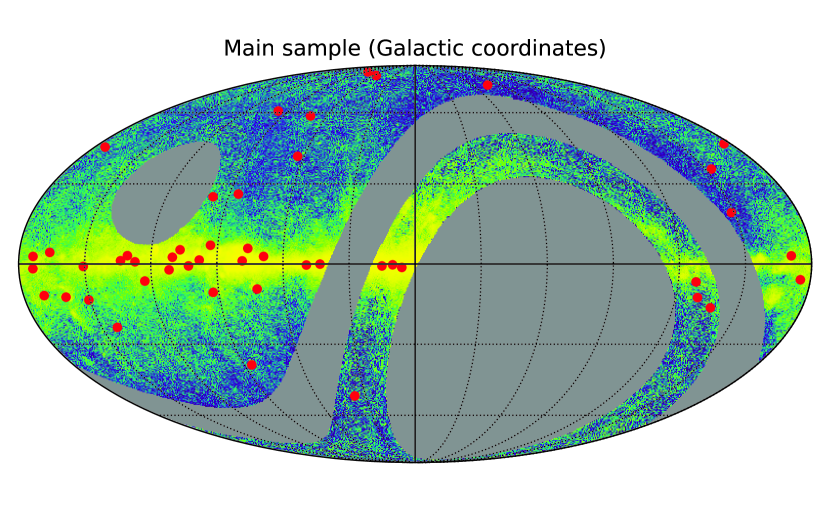
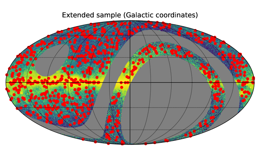
We also study a non-blind extended sample (ES) that includes the positions of the remaining PCCS2 sources detected by Planck at 30 GHz (Planck Collaboration et al., 2016) that lie in the area covered by the analysis mask proposed for the QUIJOTE MFI Wide Survey, and that are not in the main sample described above. We have used a search radius of one degree—slightly greater than the QUIJOTE FWHM at 11 GHz—to find and clean targets that may overlap at the QUIJOTE angular resolution. When a pair or group of possible repeated objects is found within this search radius, we keep only the one with the highest signal-to-noise ratio. After this cleaning procedure, we keep 725 PCCS2 targets not already included in our main sample. From these 725 sources, 145 ($20$ per cent) have Galactic latitude $|b|\leq 10^{\circ}$. We do not expect to provide high-significance polarization measurements for most of this sample; however, the total intensity measurements for these sources should be useful for filling a gap in the SEDs of many already known bright radio sources between low-frequency surveys such as the Parkes-MIT-NRAO Survey at 4.85 GHz (PMN, Wright et al., 1994), the Green Bank 6-cm radio source catalogue, also at 4.85 GHz (GB6, Gregory et al., 1996), CRATES at 8.4 GHz (Healey et al., 2007), the Owens Valley Radio Observatory (OVRO) blazar monitoring data at 15 GHz (Richards et al., 2011), or the Arcminute Microkelvin Imager (AMI) Large Array, also at 15 GHz (AMI Consortium et al., 2011), and higher frequency surveys such as the Australia Telescope 20 GHz Survey (AT20G, Murphy et al., 2010), and the WMAP (López-Caniego et al., 2007; Bennett et al., 2013) and Planck (Planck Collaboration et al., 2011, 2014, 2016, 2018) point source catalogues. The middle panel of Figure 1 shows the positions on the sky, in Galactic coordinates, of the 725 sources in the ES.

2.2 Blind search

For the blind search, sources were detected at each frequency and horn independently, using improved versions of the detection pipelines used to create the first and second Planck catalogues of compact sources (PCCS and PCCS2, Planck Collaboration et al., 2014, 2016). These pipelines are based on the Mexican Hat Wavelet 2 algorithm (MHW2, González-Nuevo et al., 2006; López-Caniego et al., 2006), which was also used to construct non-blind catalogues of sources from WMAP data (López-Caniego et al., 2007; González-Nuevo et al., 2008; Massardi et al., 2009). MHW2 is a cleaning and denoising algorithm used to convolve the maps, preserving the amplitude of the sources while greatly reducing the large-scale structures visible at these frequencies (e.g. diffuse Galactic emission) and small-scale fluctuations (e.g. instrumental noise) in the vicinity of the sources. The preservation of the amplitude of the sources after filtering with MHW2 allows us to use MHW2 not only as a detector, but as an unbiased photometric estimator of the flux density of the sources. In the following, we shall refer to this photometric estimator as MHW2 photometry.

The algorithm projects the QUIJOTE full-sky temperature maps onto square patches where the filtering and detection is performed. The sizes of the patches ($14.658\times 14.658$ deg²), and the overlap between patches has been chosen in such a way that the full sky is effectively covered. Sources above a fixed signal-to-noise ratio (SNR) threshold are selected and their positions are translated from patch to spherical sky coordinates. Because the patches overlap, multiple detections of the same object can occur; these must be found and removed, keeping the detection with the highest SNR for inclusion in the catalogue. Because the MFI instrument observes the sky at 17 and 19 GHz through two different horns, if a source is detected with both horns at those frequencies the MHW2 catalogues only keeps the detection of the horn with the higher SNR.

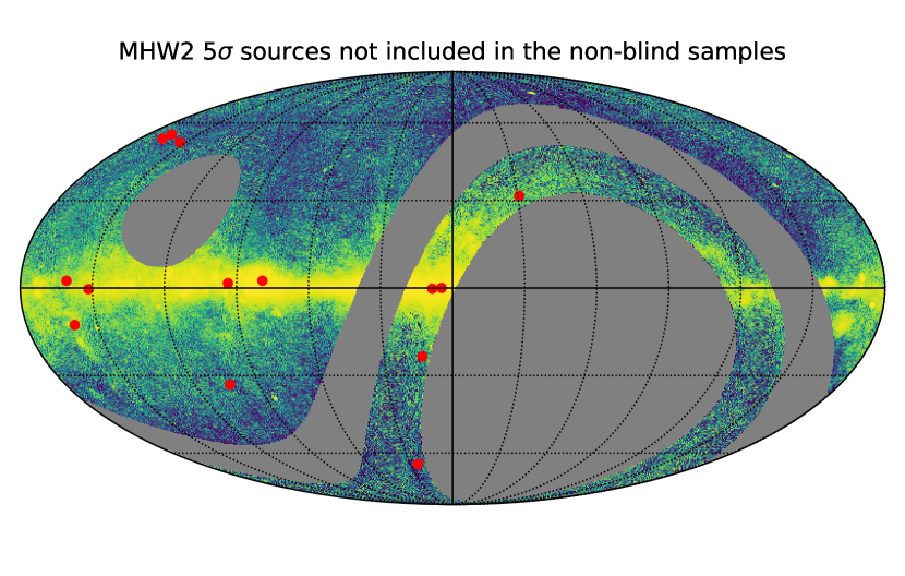
The number of sources with SNR$\geq 4$ detected by the MHW2 are 178, 179, 145, and 143 at 11, 13, 17, and 19 GHz respectively. For SNR$\geq 5$ the numbers drop to 118, 112, 74, and 50 sources at 11, 13, 17, and 19 GHz respectively. From those $5\sigma$ objects, 6, 4, 6, and 5 targets at 11, 13, 17, and 19 GHz respectively are not present in either the main sample or in the extended non-blind sample. Some of these detections correspond to the same source appearing above the $5\sigma$ level at different frequencies. In total, these 6+4+6+5 detections correspond to 14 distinct positions on the sky. The lower panel of Figure 1 indicates the positions on the sky of those 14 blind $5\sigma$ MHW2 targets. We keep their 14 unique coordinates as additional targets whose polarimetric properties will be studied with the technique described in Section 3 and that will be added to our extended sample of sources. These 14 sources may be targets not considered in the PCCS2 owing to the selection criteria followed by the Planck collaboration.

In total, we are left with 47 sources from the original main sample, 725 sources from the extended sample and 14 targets from the blind MHW2 sample, leading to 786 targets to be studied in this paper. Most of these targets have low signal-to-noise ratios in the MFI maps. Table 1 summarizes the number of sources detected in temperature (after filtering as described in Section 3.2) in our full sample (non-blind plus blind sources) above the $4\sigma$ and $5\sigma$ levels in the whole sky outside the $|b|\leq 20^{\circ}$ Galactic band.

	11 GHz	13 GHz	17 GHz	19 GHz
N($\geq 4\sigma$)	149 (83)	142 (81)	81 (22)	59 (12)
N($\geq 5\sigma$)	88 (42)	85 (38)	53 (12)	36 (8)

Table 1: Number of sources in our catalogue (blind + non-blind) detected in temperature above a given sigma level threshold in each of the MFI channels. Numbers between parenthesis indicate the number of sources above the same threshold that have Galactic latitude $b\geq 20^{\circ}$.

3 METHOD

Polarization of light is conveniently described in terms of the Stokes parameters $\mathrm{I}$, $\mathrm{Q}$, $\mathrm{U}$ and $\mathrm{V}$ (see Kamionkowski et al., 1997 for a review on CMB polarization). The parameter $\mathrm{I}$ is the total intensity of the radiation, whereas $\mathrm{Q}$ and $\mathrm{U}$ are the linear polarization parameters, and $\mathrm{V}$ indicates the circular polarization, Whereas $\mathrm{Q}$ and $\mathrm{U}$ depend on the orientation of the reference frame. The total polarization, defined as

$$\mathrm{P}\equiv\sqrt{\mathrm{Q}^{2}+\mathrm{U}^{2}},$$ (1)

is invariant with respect to the relative orientation of the receivers and the direction of the incoming signal, and therefore has a clear physical meaning. Although. properly speaking. $\mathrm{Q}$ and $\mathrm{U}$ are components of a $2\times 2$ symmetric trace-free tensor, in practice the quantity $\mathrm{P}$ can be treated as the modulus of a vector. Argüeso et al. (2009) studied the problem of the detection/estimation of a physical quantity that behaves as the modulus of a vector and is associated with a compact source embedded in stochastic noise. In particular, Argüeso et al. (2009) developed two techniques, one based on the Neyman-Pearson lemma (see, for example, Herranz & Vielva, 2010)—the Neyman-Pearson filter (NPF)—and another based on pre-filtering before fusion, the Filtered Fusion (FF), to deal with the problem of detection of the source and estimation of the polarization given two images corresponding to the $\mathrm{Q}$ and $\mathrm{U}$ components of polarization. When the source is embedded in white Gaussian noise, the NPF and the FF are both easy to implement and perform similarly well (Argüeso et al., 2009), but for non-white noises the FF technique is much easier to implement—as it basically consists of the application of two independent matched filters on the $\mathrm{Q}$ and $\mathrm{U}$ images—so for this paper we have opted to use the Filtered Fusion technique. All the results presented in the following sections have been obtained with a Python version of the IFCAPOL code, which implements the FF technique and is publicly available through the RADIOFOREGROUNDS portal. The FF method and IFCAPOL have already been used in the study of the polarization of WMAP (López-Caniego et al., 2009) and Planck (Planck Collaboration et al., 2016) sources.

3.1 Data model

Let us consider a pair of images $d_{\mathrm{Q}}$ and $d_{\mathrm{U}}$ containing a point source plus some amount of noise, where by ‘noise’ we mean any other physical or instrumental component apart from the point source itself (i.e. instrumental noise, Galactic and extragalactic foregrounds, CMB, etc.). The images could be all-sky spherical maps or local flat patches projected around a given celestial coordinate; in our experience, a local analysis helps to capture and to deal with the non-stationarity of Galactic emission, so we therefore prefer to work with flat images. Each image has been obtained through an instrument with an angular beam response $\tau_{y}(\mathbf{x})$, where $\mathbf{x})$ is the position on the sky and $y$ can take the values $\mathrm{I}$, $\mathrm{Q}$, $\mathrm{U}$ or, later on, $\mathrm{P}$ (note that the beam response does not need to be the same for the $\mathrm{I}$, $\mathrm{Q}$ and $\mathrm{U}$ images). Let us normalize the beam response so that $\tau_{y}(0)\equiv 1$, then for both images we may write

$$d_{y}(\mathbf{x})=A_{y}\tau_{y}(\mathbf{x})+n_{y}(\mathbf{x}),$$ (2)

$A_{y}$ being the amplitude of the compact source $y\in(Q,U)$ and $n_{y}(\mathbf{x})$ the corresponding noise in both components. Note that, in contrast to the situation for total intensity, where the amplitude is always positive, $A_{y}$ can have either sign depending on the polarization angle of the source.

3.2 Optimal filtering

If the noises $n_{y}$ are Gaussian (but not necessarily white) the optimal estimator for $A_{y}$ is the matched filter (Kay, 1998; Herranz & Vielva, 2010), which in Fourier space has the straightforward expression

$$\psi_{y}\left(\mathbf{k}\right)=\alpha_{y}\frac{\tau_{y}\left(\mathbf{k}\right)}{P_{y}(k)},$$ (3)

where $\mathbf{k}$ is the Fourier wave vector, $k\equiv|\mathbf{k}|$, $P_{y}(k)$ is the power spectrum of the noise $n_{y}(\mathbf{x})$ and $\alpha_{y}$ is an appropriate normalization. If we wish the filtered image to be an unbiased estimator of $A_{y}$ at the position of the source, we need

$$\alpha_{y}\equiv\left[\int d\mathbf{k}\,\frac{\tau_{y}^{2}\left(\mathbf{k}\right)}{P_{y}(k)}\right]^{-1}.$$ (4)

Equations (3) and (4) give the most frequently used version of the matched filter in CMB astronomy.

If $\tilde{d}_{\mathrm{Q}}(\mathbf{x})$ and $\tilde{d}_{\mathrm{U}}(\mathbf{x})$ are the filtered images for the $\mathrm{Q}$ and $\mathrm{U}$ Stokes parameters and we have a source located at $\mathbf{x}=0$, then $\tilde{d}_{\mathrm{Q}}(0)$ and $\tilde{d}_{\mathrm{U}}(0)$ are the optimal linear estimators of the amplitudes $A_{\mathrm{Q}}$ and $A_{\mathrm{U}}$, ‘optimal’ meaning here that

• $\tilde{d}_{y}(0)$ is an unbiased estimator of $A_{y}$; that is, $\langle\tilde{d}_{y}(0)\rangle=A_{y}$. The operator $\langle\cdot\rangle$ indicates an ensemble average.

• The ensemble variance $\sigma^{2}_{\tilde{d}}$ is minimum.

The first of these two properties means that the matched filter can be used as an unbiased photometric estimator of the flux density of the sources, both in temperature and in the Q and U Stokes parameters. The r.m.s. of the filtered image in an annulus around the position of the sources can be used as an estimator of the uncertainty of the matched filter photometry. Particular details about the size of the images and the annulus for this data set can be found in Section 3.5. Unless stated otherwise, all the I, Q and U values, and their corresponding uncertainties provided in this paper are obtained using matched filter photometry (MF photometry).

3.3 Estimation of $\mathrm{P}$

Once we have estimated the $\mathrm{Q}$ and $\mathrm{U}$ flux densities by means of the matched filters, we can construct a fusion-filtered map of $\mathrm{P}$ as

$$\tilde{d}_{\mathrm{P}}(\mathbf{x})=\sqrt{\tilde{d}^{2}_{\mathrm{Q}}(\mathbf{x})+\tilde{d}^{2}_{\mathrm{U}}(\mathbf{x})}.$$ (5)

For economy, let us change our notation a little so that

$$\tilde{\mathrm{Q}}\equiv\tilde{d}_{\mathrm{Q}}(0)$$ (6)

and

$$\tilde{\mathrm{U}}\equiv\tilde{d}_{\mathrm{U}}(0).$$ (7)

Then, over an ensemble of realizations, $\langle\tilde{\mathrm{Q}}\rangle=A_{\mathrm{Q}}$ and $\langle\tilde{\mathrm{U}}\rangle=A_{\mathrm{U}}$. It is straightforward to get the following estimator of $\mathrm{P}$:

$$\tilde{\mathrm{P}}\equiv\sqrt{\tilde{\mathrm{Q}}^{2}+\tilde{\mathrm{U}}^{2}}.$$ (8)

Unfortunately, this is a biased estimator of the amplitude of the polarization $A_{\mathrm{P}}$ of a source (see for example Montier et al., 2015). Argüeso et al. (2009) studied the bias of the FF estimator (8), showing that it is easy to control for detectable sources. For uncorrelated noises and assuming for simplicity that both images have the same r.m.s. noise level (for the QUIJOTE MFI Wide Survey maps this is a reasonable assumption), the relative bias can be shown to behave as

$$\frac{\tilde{\mathrm{P}}-A_{\mathrm{P}}}{A_{\mathrm{P}}}\simeq\frac{1}{\mathrm{SNR}_{\mathrm{Q}}^{2}+\mathrm{SNR}_{\mathrm{U}}^{2}},$$ (9)

where SNR_y is the signal-to-noise ratio of the source for the Stokes parameter $y$ after filtering. This means that if the source is detectable at the $3\sigma$ level in at least $\tilde{\mathrm{Q}}$ or $\tilde{\mathrm{U}}$ the relative bias should be less than or equal to $\sim$10%, and if at least one of them is at the $5\sigma$ level the relative bias would be $\leq 4\%$. In practice, the bias will be negligible for the brightest sources. In any case, the noise bias can be removed by subtracting the corresponding noise contributions $\sigma_{\tilde{\mathrm{Q}}}^{2}$ and $\sigma_{\tilde{\mathrm{U}}}^{2}$ from the filtered $\tilde{\mathrm{Q}}^{2}$ and $\tilde{\mathrm{U}}^{2}$ images . As noted by López-Caniego et al. (2009), this correction turns out to be negligible in most cases. We shall provide the debiased polarized flux density as

$$\tilde{\mathrm{P}}_{\mathrm{debiased}}=\sqrt{\tilde{\mathrm{P}}^{2}-\sigma_{\tilde{\mathrm{P}}}^{2}},$$ (10)

where $\sigma_{\tilde{\mathrm{P}}}$ is the error in $\tilde{\mathrm{P}}$ and is calculated by propagating the errors in $\tilde{\mathrm{Q}}$ and $\tilde{\mathrm{U}}$. The standard deviations $\sigma_{\tilde{\mathrm{Q}}}$ and $\sigma_{\tilde{\mathrm{U}}}$ are calculated as the local r.m.s. in an annulus around the source in the matched filtered $\tilde{\mathrm{Q}}$ and $\tilde{\mathrm{U}}$ maps. Then, under the assumption of no correlation:

$$\sigma_{\tilde{\mathrm{P}}}=\sqrt{\frac{\tilde{\mathrm{Q}}^{2}\,\sigma_{\tilde{\mathrm{U}}}^{2}+\tilde{\mathrm{U}}^{2}\,\sigma_{\tilde{\mathrm{Q}}}^{2}}{\tilde{\mathrm{Q}}^{2}+\tilde{\mathrm{U}}^{2}}}.$$ (11)

Even if the noises $n_{\mathrm{Q}}(\mathbf{x})$ and $n_{\mathrm{U}}(\mathbf{x})$ are Gaussian-distributed, the noise residual after the filtered fusion is not Gaussian. Rather than working with the usual signal-to-noise ratio, it is more appropriate to report the statistical significance of the detection of $\mathrm{P}$; that is, one minus the probability that a given estimated signal is the product of random noise fluctuations. We compute the statistical significance by obtaining histograms of the $\tilde{d}_{\mathrm{P}}$ values, as described in López-Caniego et al. (2009).

3.4 Estimation of the polarization angle

From the filtered $\mathrm{Q}$ and $\mathrm{U}$ images we can estimate the angle of polarization of a source located at $\mathbf{x}=0$ as

$$\tilde{\phi}=\frac{1}{2}\arctan\left[-\frac{\tilde{\mathrm{U}}}{\tilde{\mathrm{Q}}}\right].$$ (12)

The QUIJOTE MFI maps use the COSMO polarization convention. The minus sign in equation (12) is inserted to obtain the $\tilde{\phi}$ angle in the IAU convention, so that we can compare it with other experiments. Assuming no correlation between the errors in $\tilde{\mathrm{Q}}$ and $\tilde{\mathrm{U}}$,

$$\sigma_{\tilde{\phi}}=\frac{1}{2\left(\tilde{\mathrm{Q}}^{2}+\tilde{\mathrm{U}}^{2}\right)}\sqrt{\tilde{\mathrm{Q}}^{2}\,\sigma_{\tilde{\mathrm{U}}}^{2}+\tilde{\mathrm{U}}^{2}\,\sigma_{\tilde{\mathrm{Q}}}^{2}}.$$ (13)

3.5 Implementation

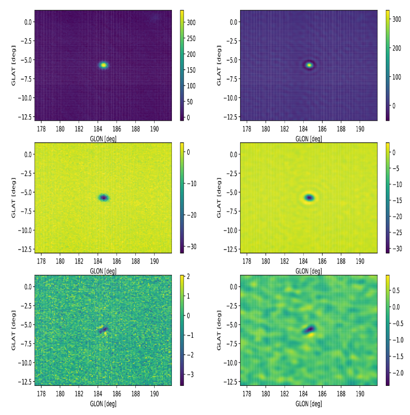
The IFCAPOL version used for this work produces flat patches of $128\times 128$ pixels using the Gnomonic projection integrated in the Python healpy package (Zonca et al., 2019) based on the HEALPix (Hierarchical Equal Area isoLatitude Pixelation of a sphere, Górski et al., 2005). For nside = 512 HEALPix maps, each pixel has an angular resolution of 6.87 arcmin; that is, each patch covers an area of $14.658\times 14.658$ deg². The FF uses an isotropic, non-Gaussian model of the beam response $\tau(\mathbf{x})$ obtained from the window functions described in Génova-Santos et al. (2023). The mean and r.m.s. values used for SNR calculations and $\tilde{\mathrm{P}}$ debiasing are calculated in rings with inner radius 2.5 times the nominal FWHM of the beam and with an outer radius equal to 6 degrees. The significance of $\tilde{\mathrm{P}}$ is calculated over all the pixels of the image, except for a 5-pixel band in the borders of the image (to avoid filtering border effects) and a mask that covers the $2.5\%$ fraction of brightest pixels of the image outside the area occupied by the source (in a similar way to López-Caniego et al., 2009, but with a more conservative criterion for masking bright pixels) to prevent contaminated pixels from being used in the calculation of the background distribution. This means that in the best case the reliability of a detection cannot be ascertained to a level higher than $99.993\%$. Figure 2 shows an example of a patch located around the Crab nebula in I, Q and U before (left panels) and after (right panels) filtering. Ringing effects around bright sources, such as those observed in the filtered Q map, are a side effect of filtering. For this reason, an annulus around the sources is used, as mentioned at the beginning of this section. The lobes in the U map is an instrumental effect associated with intensity-to-polarization leakage due to the difference between the two co-polar beams, as explained in section 9.3 of Rubiño-Martín et al. (2023). These are visible in this case because most of Crab polarized emission is contained in the Q direction in Galactic coordinates.

Figure 2: Intensity and polarization maps at 19 GHz centred on the position of the Crab nebula. The upper left- and right-hand panels show, respectively, the maps of $\mathrm{I}$ and $\tilde{\mathrm{I}}$ before and after filtering with the matched filter, while the middle panels show the analogous $\mathrm{Q}$ and $\tilde{\mathrm{Q}}$ maps. The lower panels show, for the same source, the maps of $\mathrm{U}$ and $\tilde{\mathrm{U}}$.

The polarization angle is calculated using Equation (12). Since the noise can easily change the sign of $\mathrm{Q}$ or $\mathrm{U}$, and hence $\hat{\phi}$, in cases of very low SNR sources, this implementation IFCAPOL tries automatically to homogenize the sign of $\tilde{\phi}$. It does this via the following ad hoc rule: for a given source, the sign of its polarization angle for all frequencies in the final catalogue is forced to be equal to the sign of the median value of the polarization angles at 11, 13, 17 and 19 GHz as calculated using Equation (12). This is a brute force solution; however, it is necessary since only four sources in the main sample have SNR $\geq 1.0$ in both $\mathrm{Q}$ and $\mathrm{U}$ at all frequencies. All these four sources have Galactic latitude $|b|<10^{\circ}$. These sources are listed in Table 2.

PCCS2 ID	Other ID	RA [deg]	DEC [deg]
PCCS2 030 G184.54-05.78	Crab	83.63	22.01
PCCS2 030 G130.72+03.08	3C058	31.40	64.82
PCCS2 030 G189.07+03.02	IC443	94.30	22.55
PCCS2 030 G068.83+02.80	CTB 80	298.31	32.92

Table 2: List of highly polarized sources in the main sample. These sources have SNR $\geq 1.0\sigma$ in $\mathrm{Q}$ and $\mathrm{U}$ at all MFI frequencies.

3.6 Spectral indexes

In order to obtain the estimates of the spectral indexes based on internal QUIJOTE MFI data only, it is important to include colour corrections in the analysis. Even though these are small corrections (of order of one per cent) they might bias the spectral index estimate given the small frequency range considered (11 to 19 GHz). The MFI procedure to obtain colour corrections is described in section 8.2 of Génova-Santos et al. (2023) and implemented by the fastcc (faster computation of the colour correction for a given spectral index) code (Peel et al., 2022). For point sources in this paper, we consider the spectral behaviour of bright radio sources to be well described by a single power law within the MFI frequency range. We follow an iterative procedure according to this scheme:

1. For each source, we take the four photometric points (I or P at 11, 13, 17 and 19 GHz) and their corresponding uncertainties as an initial estimate.

2. We then get an estimate of the spectral index by a weighted fitting of the points to a power law.

3. Using the estimated spectral index, we compute the colour correction factors for the four frequencies.

4. We apply these corrections to the non-colour-corrected I or P points and repeat the process from step ii. We iterate until the resulting spectral index stabilizes to within a $10^{-6}$ tolerance.

The process typically requires 5–7 iterations to achieve the requested tolerance on the spectral index. MFI colour corrections are typically small. For the Stokes parameter I, the largest effect occurs at 11 GHz, with corrections of up to $\sim$3% for sources with spectral indices between $-1$ and $+1$. This correction remains below $\sim$0.5% for 13 GHz and below $\sim$1% for 17 and 19 GHz, for the same spectral index range. Similar values are obtained for Q, U and P.

As a consistency check, we have implemented an independent method to fit for the spectral index, using a Bayesian approach that includes the simultaneous evaluation of the colour correction factors within the computation of the posterior distribution for the spectral index. As in our default methodology, flux densities are fitted to a power law, $S(\nu;A_{0},\alpha)=A_{0}\left(\nu/\nu_{0}\right)^{\alpha}$ (normalized at $\nu_{0}=$10 GHz). This approach is applied only to the intensity signal in order to validate the previous results (spectral indexes and colour correction factors). The posterior distribution for the spectral index is sampled using emcee, (Foreman-Mackey et al., 2013) following the methodology explained in Lopez-Caraballo et al. (2023). A uniform prior on $\alpha$ between $-$4 and 3 is adopted. For each source, the full posterior distribution function (PDF) is characterized with 32 chains and 10 000 iteration steps. Then, $\alpha$ and $A_{0}$ are estimated from the 50th percentile of the marginalized PDFs, while their uncertainties are estimated from the 16th and 84th percentiles. In addition, the full PDFs are a useful and complementary tool in the statistical description of our sources (see Sect. 10). The results of this second method (MCMC sampler) are virtually identical to those obtained with the iterative power-law fitting described above. Small differences arise from the parameter estimation methods, since the latter estimates the parameters as the best-fitting value (corresponding to the maximum of the PDF) while the former obtains them from the median. The mean difference between spectral indexes is $-0.07$ with a standard deviation of 0.08, where the biggest difference is $-0.47$. However, we note that the MCMC analysis generally provides greater uncertainties, which on average are a factor 2.57 higher.

Concerning the impact of colour correction on the estimation of the spectral indices of the sources, we find that the average difference between colour-corrected $\alpha$ and non-colour-corrected $\alpha$ is 0.06, which is smaller than the average $\alpha$ uncertainties of 0.39 (using the MCMC results). Although this effect is small, it may have a significant impact on the extrapolation of flux densities to lower or higher frequencies. The subsequent analysis will therefore be done using the colour-corrected flux densities.

4 Description and validation of the data products

4.1 Format of the data products

The QUIJOTE MFI Wide Survey point source catalogue is available from the RADIOFOREGROUNDS web site. It comprises two catalogue FITS files, one for our main sample, containing 47 targets, and other for our extended sample, containing 739 targets. We summarize here the catalogue contents:

• Source identification: a numerical identifier containing the string ‘MFI-PSCm’ for the main sample and ‘MFI-PSCe’ the extended sample.

• Position: GLON and GLAT contain the Galactic coordinates, and RA and DEC give the same position in equatorial coordinates (J2000).

• Stokes parameters: I, Q and U in Jy, and their associated uncertainties, for the four MFI frequencies (11, 13, 17 and 19 GHz). Values are not colour-corrected. Colour-corrections can be obtained using the public fastcc code (Peel et al., in preparation).

• Polarization: debiased P and its associated uncertainty in Jy for the four MFI frequencies (11, 13, 17 and 19 GHz). Values are calculated from the raw (non-colour-corrected) Stokes parameters.

• Polarization fraction and its associated uncertainty for the four MFI frequencies, as calculated from debiased P and I.

• Polarization angle: $\phi$ and its associated uncertainty, in degrees, for the four MFI frequencies (11, 13, 17 and 19 GHz). The polarization angles are defined as increasing anticlockwise (north through east) following the IAU convention; the position angle zero is the direction of the north Galactic pole.

• Statistical significance of the detection of the polarized signal, for the four MFI frequencies.

• Spectral index in intensity: column ALPHA_I gives the colour-corrected spectral index calculated as described in section 3.6. Its associated error is given in column ALPHA_I err.

• Spectral index in polarization: column ALPHA_P gives the colour-corrected spectral index calculated as described in section 3.6. Its associated error is given in column ALPHA_P err.

• Flag: source candidates with estimated $\mathrm{SN}R<0$ in at least one frequency are flagged with the number 1. For these sources, the corresponding I column has been set to NaN. The corresponding uncertainty is kept as it may be used as an upper flux density limit estimate. We do not provide spectral index estimates for these sources, as they are considered as only marginal detections. There are 14 of these sources in the extended catalogue and zero in the main catalogue. The rest of sources are flagged with the value 0.

• Cross-identifications: where possible, we give the name of possible cross-identifications, within a $30^{\prime}$ search radius around the position of each MFI source candidate, to the following surveys of radio sources:

  • PCCS2 ID: nearest matched source in the Planck Second Catalogue of Compact Sources (Planck Collaboration et al., 2016).

  • PNCT ID: nearest matched source in the Planck Catalogue of Non-Thermal Sources (Planck Collaboration et al., 2018).

  • Other IDs: for those cases where it is possible, we also give the nearest match, within a $30^{\prime}$ search radius, to the 3C (Bennett & Simth, 1962) and the Parkes-MIT-NRAO (PMN, Wright et al., 1994) surveys of radio sources.

4.2 Internal consistency

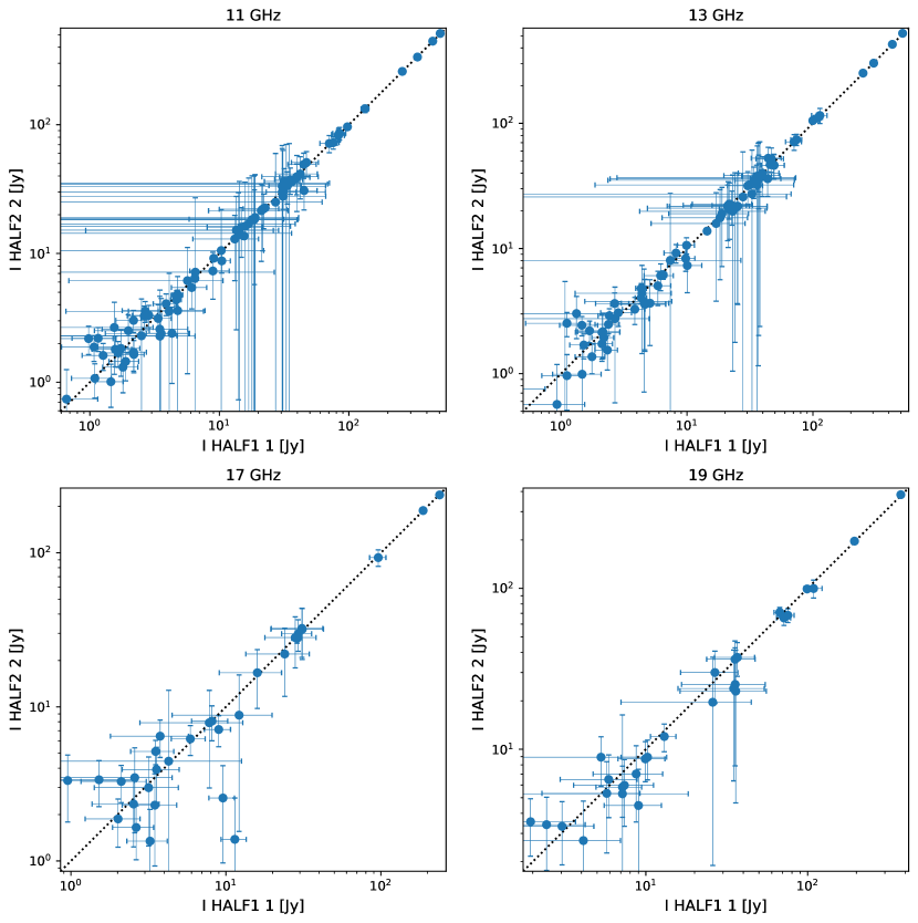
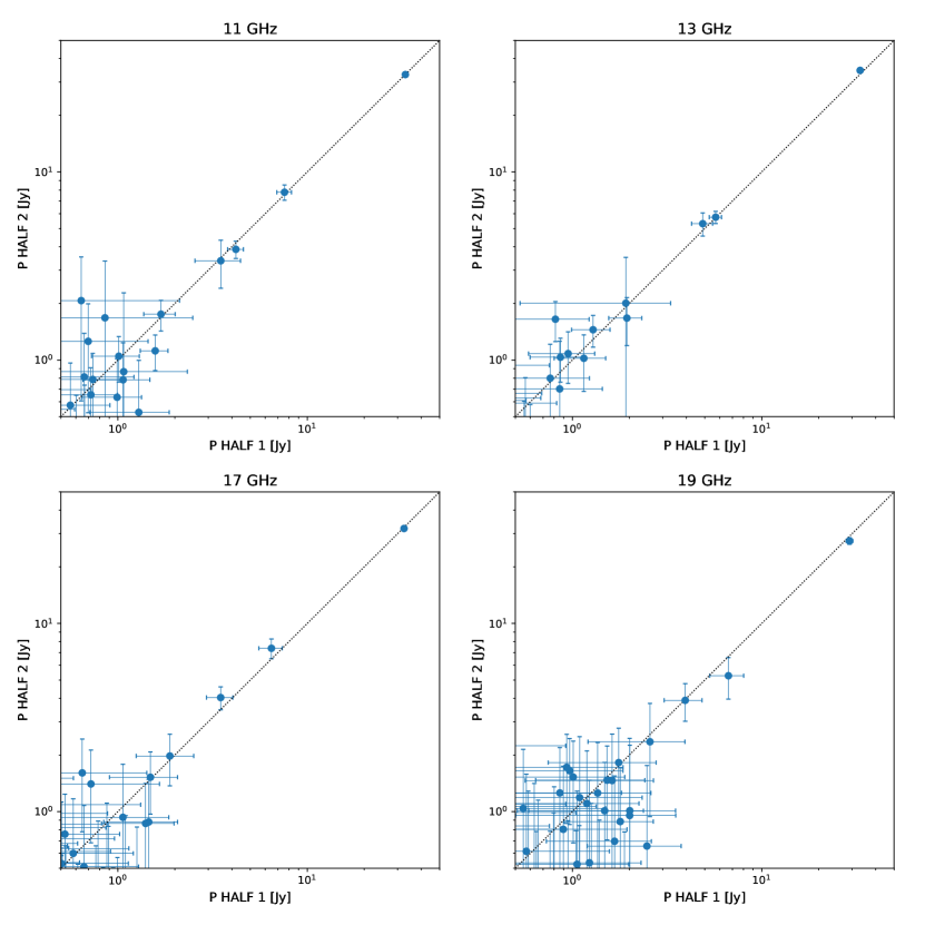
In order to check the self-consistency of IFCAPOL, as well as have at hand an additional means of testing the stability of QUIJOTE data and the map-making algorithm (see Gómez-Reñasco et al., 2012; Pérez-de-Taoro et al., 2016; Rubiño-Martín et al., 2023; Génova-Santos et al., 2023), we have conducted a series of jackknife tests comparing the estimation of the main photometric and polarimetric quantities ($\mathrm{I}$, $\mathrm{P}$ and $\phi$, but also $\mathrm{Q}$ and $\mathrm{U}$ individually) on two different maps, which have been produced by splitting the MFI wide survey data into two halves. The maps that we use are the so-called ‘half-mission maps’ and they are constructed by separating the individual observations (6 h each) according to the calendar date in each observing period (there are four in total, spread over 6 yr) and each telescope elevation (usually we have three or four observing elevations in each period). A more complete description of these maps is given in Rubiño-Martín et al. (2023). By construction, these maps are designed to have almost identical sky signal and sky coverage, but independent noise. Note that by design, the effective epoch of the two half-mission maps is almost identical. We use specific versions of these half-mission maps that have been generated with our map-making algorithm (PICASSO, Guidi et al., 2021) using the common baseline reconstruction as for the full map (Rubiño-Martín et al., 2023). This guarantees a better rejection of $1/f$ noise in the two halves, which benefits the analyses that are presented in this section.

Figures 3, 4 and 5 show how the two half-survey maps compare when we estimate $\mathrm{I}$, $\mathrm{P}$, and $\phi$ respectively. In order to reduce spurious scatter from the use of different horns, only values that have been obtained using the same MFI horn are used for the plots. An additional cut requiring that the measurement of P has statistical significance $\geq 0.68$ in the full map has been applied for the comparison. The numbers of sources satisfying the above requirements, and are therefore used for the fit, are 81, 75, 31 and 26 for 11, 13, 17 and 19 GHz respectively. A summary of the results of a linear fit between the estimates obtained with the first and the second half-survey is presented in Table 3. The I and P estimations show good concordance between the subsets used for this test. The 17 and 19 GHz channels have fewer samples and show a wider scatter than the lower frequencies, probably because steep-spectrum sources decrease quickly in flux density as the observation frequency increases. Both half-survey maps show similar sensitivities, as expected since each of them corresponds to the same number of samples. This is confirmed by the size of the error bars and by a quantitative analysis of these uncertainties, which shows no statistically significant discrepancies between both half-survey maps.

Freq [GHz]	I [Jy]	P [Jy]	$\phi$ [deg]
11	$(0.996\pm 0.008)x+(0.07\pm 0.13)$	$(0.99\pm 0.02)x-(0.00\pm 0.03)$	$(1.00\pm 0.01)x-(0.2\pm 0.8)$
13	$(1.002\pm 0.008)x+(0.08\pm 0.14)$	$(1.04\pm 0.02)x-(0.02\pm 0.04)$	$(1.00\pm 0.01)x+(0.0\pm 0.8)$
17	$(0.996\pm 0.014)x-(0.4\pm 0.4)$	$(0.89\pm 0.15)x+(0.02\pm 0.09)$	$(1.03\pm 0.05)x-(5.0\pm 3.0)$
19	$(1.015\pm 0.010)x-(0.4\pm 0.9)$	$(1.01\pm 0.04)x-(0.09\pm 0.14)$	$(1.21\pm 0.04)x+(16.0\pm 3.0)$

Table 3: Fit coefficients between the first and second half-survey maps for the total intensity, polarization and polarization angle of the main sample catalogue.

Figure 3: Comparison of $\mathrm{I}$ estimation in the two MFI Wide Survey half-surveys. The black dotted line indicates the equality $y=x$.

Figure 4: Comparison of $\mathrm{P}$ estimation in the two MFI Wide Survey half-surveys. The black dotted line indicates the equality $y=x$.

Figure 5: Comparison of the polarization angle estimation in the two MFI Wide Survey half-surveys, shown as a density plot.

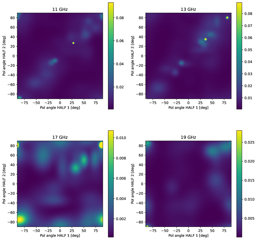
Regarding the polarization angle, the estimated angles show large error bars and, even after the homogeneization process described in Section 3.5, a significant scatter. Error-bar diagrams such as those shown in Figures 3 and 4 become very cluttered by the error bars and difficult to read. We have chosen instead to show a density diagram in Figure 5. For this diagram, each point has been substituted by a normalized Gaussian ellipsoid with semiaxis equal to the estimated polarization angle error. Well-determined polarization angles create dense knots in this diagram, whereas sources with a large uncertainty form very spread out clouds. There is a clear linear trend at 11, 13 and, to a lower extent, 17 GHz. There is a cluster of sources with switched angle in the upper left corner of the plot at 19 GHz. The reason for this is that when either $\mathrm{Q}$ or $\mathrm{U}$ is small, random noise fluctuations can change the sign or the semi-quadrant of $\tilde{\phi}$. This is particularly dangerous for sources with polarization angle near $\pm 90$ degrees. If we artificially force the signs of angles whose absolute value is larger than 80 degrees to agree, the 19 GHz fit becomes $\tilde{\phi}_{H2}=(0.95\pm 0.02)\tilde{\phi}_{H1}-(7.59\pm 2.04)$. Here the H1 and H2 subscripts denote the first and second half-mission maps respectively. In any case, Figure 5 indicates that polarization angle estimates at 17 and 19 GHz are less reliable than those at 11 and 13 GHz.

4.3 MF versus MHW2 photometry

As mentioned in Sections 2.2 and 3.5, both filters used for the non-blind (MF) and blind (MHW2) samples are, from a statistical point of view, detectors and estimators of the flux density of the sources at one and the same time. We use the MF photometry for all the products that come with this paper, except for the number-count analysis to be described in Section 5.1, where we have opted to keep the native MHW2 photometry of the blind sample for statistical consistency. It is still interesting to test whether the MHW2 and the MF photometries are compatible. We have fitted the MF estimated intensity versus the corresponding MHW2 photometry for all the matches between the blind and non-blind sources, taking into account the photometric uncertainties in both axes. Since all the detections are internal to the QUIJOTE MFI (we are not comparing with external catalogues), here we allow the matching radius to be roughly equal to the FWHM of the best-resolution MFI channel ($\sim$35 arcmin at 17 and 19 GHz). Table 4 shows the linear-fit parameters and their uncertainties for sources with $\mathrm{SNR}\geq 5$. The agreement is remarkable. Since both photometries have been obtained with two totally independent codes and the MHW2 has been well tested in other experiments such as WMAP and Planck, we take this result as an additional validation of our photometry.

Freq [GHz]	$a$	$b$ [Jy]
11	$1.01\pm 0.01$	$0.01\pm 0.07$
13	$1.00\pm 0.01$	$0.01\pm 0.07$
17	$1.02\pm 0.01$	$-0.42\pm 0.21$
19	$1.01\pm 0.01$	$-0.40\pm 0.43$

Table 4: Parameters of the fit $\mathrm{I}_{\mathrm{MHW2}}=a\,\mathrm{I}_{\mathrm{MF}}+b$ between the MHW2 photometry and the MF photometry, for all the sources in the blind sample that are matched within a 35 arc minutes search radius to a $\mathrm{SNR}\geq 5$ source in the non-blind sample.

4.4 Calibrators

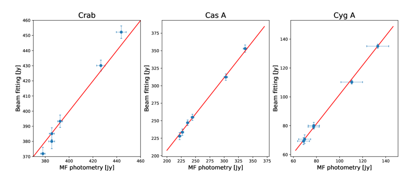
The main amplitude calibrator of the QUIJOTE MFI Wide Survey is the Crab supernova remnant (Tau A), while the supernova remnant Cassiopeia A (Cas A) and the radio galaxy 3C405 (Cygnus A) are used for consistency tests. This calibration is based on beam-fitting photometry, performed at either the time-ordered data or at the map level—see details in Rubiño-Martín et al. (2023), and a general description of the QUIJOTE MFI calibration in Génova-Santos et al. (2023). Comparison of the reference flux densities of these sources at the MFI frequencies, given by the external models that were used for calibration, is a very useful validation test of our methodology, which relies on a different and independent kind of photometry.

Figure 6 shows the photometric measurements used for this paper as compared to the prediction from the models that were used to calibrate the MFI real-space beam-fitting photometry in Rubiño-Martín et al. (2023) and Génova-Santos et al. (2023). The red line line shows the best linear $y=a\,x$ fit. The agreement to a linear law is good, particularly for Cas A and Cyg A. The linear fit gives slopes of $0.999\pm 0.005$, $1.039\pm 0.008$ and $1.015\pm 0.031$ for Crab, Cas A and Cyg A respectively. The compelling agreement for the Crab is not surprising, as this source has been used as our main calibrator (Génova-Santos et al., 2023). If we compute the percentage relative residuals between the two photometries as

$$r=100\left|\frac{I-I_{bf}}{I_{bf}}\right|,$$ (14)

where $I$ is the flux density estimated in this paper and $I_{bf}$ is the beam fitting photometry described in Génova-Santos et al. (2023), we get $1.05\%$ mean (from the four frequencies) relative errors for the Crab, $3.56\%$ for Cas A and $1.47\%$ for Cygnus A. The three values are below the $\sim$5 per cent calibration uncertainty of the MFI maps.

Figure 6: Comparison between the beam-fitting photometry used for the Wide Survey map calibration (Rubiño-Martín et al., 2023) and the MF photometry used in this paper for the six MFI detectors (corresponding to horns 2, 3 and 4) and for the three calibration sources Crab, Cassiopeia A and Cygnus A. The red line line shows the best linear $y=a\,x$ fit.

As an additional consistency test for the MF photometry, we have extended the same real-space beam-fitting procedure to the whole catalogue. We find agreements between the two photometries that are roughly similar to the agreement between the MF and the MHW2 estimates discussed in the previous section. As an example, at 11 GHz we find slope $a=1.05$ and intercept $b=-0.25$.

4.5 VLA observations

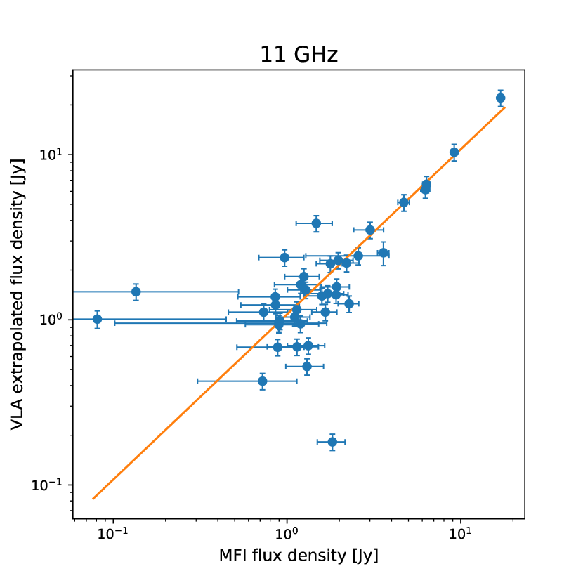
In parallel to the observation of the QUIJOTE-MFI Wide Survey, and as a part of the European Union’s Horizon 2020 RADIOFOREGROUNDS project, Perrott et al. (2021) observed a sample of 51 sources with the Very Large Array at 28–40 GHz. These sources are located in the QUIJOTE cosmological fields and are brighter than 1 Jy at 30 GHz in the Planck Point Source Catalogue. The observations were to characterize their high radio-frequency variability and polarization properties. The sources were observed with a custom correlator configuration that allowed simultaneous observations at two frequency bands, 28.5–32.4 and 35.5–39.4 GHz, which were divided into 32 spectral windows, each with 64 channels of width 2 MHz. Using this configuration, Perrott et al. (2021) measured the total intensity flux density and spectral index at $\sim$34 GHz of these 51 sources, as well as their polarimetric properties (polarization fraction and angle, rotation measure). Since those observations partially overlap in time with the QUIJOTE MFI Wide Survey observations, the VLA sample provides a good additional testbed for the MFI point source catalogues. There are 49 matches (within a 30^′ search radius) between the Perrott et al. (2021) VLA sample and the sum of our main and extended MFI catalogues. For this matching, we have considered only those VLA sources observed during the MFI Wide Survey observation campaign (May 2013 to June 2018). Five of the sources in our main+extended catalogue are resolved or have multiple images in the VLA maps (that is, they can be associated with more than one VLA source within the 30^′ matching radius). We have not included these sources in the following analysis. This leaves 39 matches between our catalogue and the VLA sample. Using the VLA 34 GHz estimated flux density and spectral index, we have extrapolated the total intensity flux density of these 39 matches to MFI frequencies, assuming a single power law frequency dependence. Figure 7 shows the comparison between the MFI (colour-corrected) flux density at 11 GHz $S_{\mathrm{MFI}}^{11}$ and the VLA-extrapolated flux density at the same frequency $S_{\mathrm{VLA}}^{11}$ for the 39 sources in the cosmological field studied by Perrott et al. (2021) that are in our catalogues. A fit to the law $S_{{\scriptscriptstyle\mathrm{VLA}}}^{11}=a\,S_{{\scriptscriptstyle\mathrm{MFI}}}^{11}$ gives $a=1.08\pm 0.04$. The agreement is remarkable considering the frequency gap between 11 and 34 GHz, the different systematics that affect the VLA and the QUIJOTE MFI, and source variability.

Figure 7: Comparison between the QUIJOTE MFI flux density at 11 GHz and the flux density extrapolated from VLA observations at 34 GHz for 39 sources in the QUIJOTE cosmological fields (Perrott et al., 2021). The orange solid line shows the best linear fit.

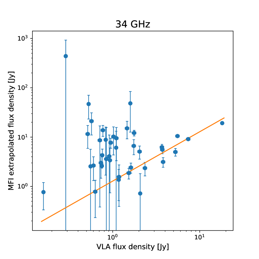
It is also interesting to repeat the same exercise in the opposite way. We have used the MFI flux densities at 11, 13, 17 and 19 GHz to fit an intensity and spectral index that we have used to predict the flux density of the sources at the VLA average frequency of 34 GHz. Figure 8 shows the results of this exercise. MFI predictions tend to overestimate the flux density at 34 GHz for sources below $\sim$10 Jy. The fit $S_{\scriptscriptstyle\mathrm{MFI}}^{34}=b\,S_{{\scriptscriptstyle\mathrm{VLA}}}^{34}$ gives $b=1.29\pm 0.04$. As expected, the VLA observations give more precise spectral index estimates than the MFI data owing to the difference in sensitivity.

Figure 8: Comparison between VLA observations at 34 GHz for 39 sources in the QUIJOTE cosmological fields (Perrott et al., 2021) and the predicted flux at the same frequency using spectral index fitted from the QUIJOTE MFI data at 11, 13, 17 and 19 GHz. The orange solid line shows the best linear fit.

5 Intensity and polarization properties of the sources

5.1 Number counts in total intensity

Figure 9: Differential source number counts (blue dots) for the MHW2 blind sample at 11, 13, 17 and 19 GHz. Only sources with $\sigma\geq 4.5$ and outside the Galactic mask have been used for this plot. As a comparison, the predicted radio source number counts from the De Zotti et al. (2005) model are also plotted (continuous orange line).

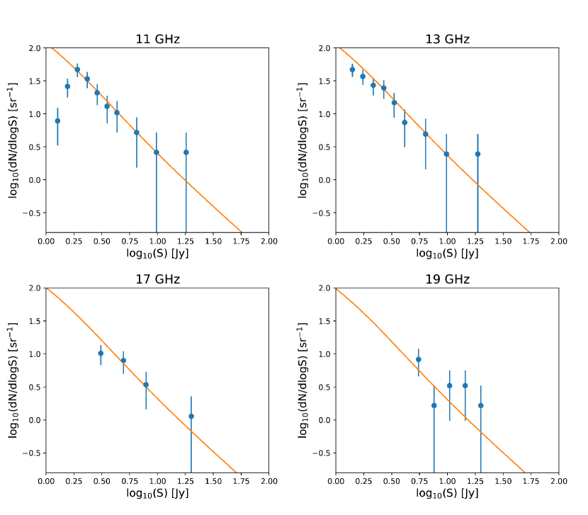
Counts of radio galaxies are one of the traditional ways of characterizing the evolutionary properties of this type of extragalactic object. However, to study properly the evolution of radio sources we would need to go to flux density limits that are well below QUIJOTE’s sensitivity. Nevertheless, number counts are still interesting as a means of checking the validity of our point source catalogue by comparing its number counts with well-known models. For this purpose the catalogue needs to be blind, so we focus on the MHW2 sources described in Section 2.2. We use the flux densities obtained by the MHW2, knowing that they are consistent with the MF photometry used in the rest of the paper (see Section 4.3). We have considered only bright sources (detected at the $\geq 4.5\sigma$ level in each channel) likely to be extragalactic (outside the GAL070 Planck Galactic mask). We have not applied any colour correction to these sources. The reason for this decision is that in order to compute colour corrections we need to estimate spectral indexes for the sources and this can be done only for the intersection of the single-frequency catalogues; this would further reduce the size of our sample, so we prefer to keep the full blind MHW2 catalogues at each frequency, Figure 9 shows the differential number counts for the sources satisfying the above conditions at 11, 13, 17 and 19 GHz (blue dots). The solid orange line shows the number count models by De Zotti et al. (2005) at these frequencies (the updated counts models by Tucci et al. (2011) are essentially identical to the De Zotti et al. (2005) models for frequencies below 30 GHz). At 11 and 13 GHz the agreement between the MFI MHW2 blind catalogue differential source number counts and the De Zotti et al. (2005) models is remarkably good and indicates a $4.5\sigma$ completeness limit $\sim 1.8$ Jy. At 17 and 19 GHz the agreement with the De Zotti et al. (2005) model is also reasonably good, but one must take into account that the number of $4.5\sigma$ sources outside the Galactic mask at these frequencies is too low to give reliable statistics. The number of sources used for the plots in Figure 9 are 67, 70, 21 and 13 for 11, 13, 17 and 19 GHz respectively.

5.2 Spectral indexes in total intensity

Figure 10: Spectral index distribution of sources in the extragalactic (red) and the Galactic (blue) sample. Extragalactic sources are located in the sky region observed by the Planck GAL040 Galactic mask (outside the masked area), while the Galactic sources are in the complementary area (inside the masked area). For each sample, the histogram and probability density function (dashed lines) are shown. The area under the histograms and the probability density functions integrate to 1 (normalized). The grey dotted line establishes the $\alpha=-0.5$ limit used to separate flat ($\alpha>-0.5$) and steep ($\alpha\leq-0.5$) spectrum sources.

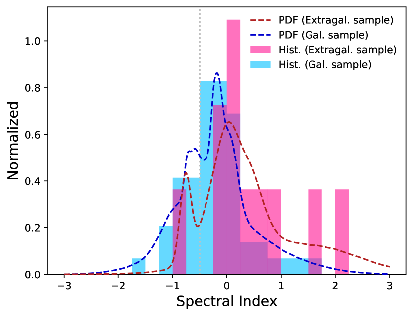
The distribution of spectral indexes is shown in Figure 10. We have considered the spectral indexes only for sources detected above the 3$\sigma$ level in all the frequencies simultaneously, which amounts to 69 sources. This means that only bright sources, $S\geq 1$ Jy at 11 GHz, are studied in Figure 10. In principle, we can distinguish between Galactic and extragalatic sources depending on whether they are inside or outside the masked area of the GAL40 Galactic mask respectively. The GAL40 mask is more restrictive than the GAL70 mask used in the previous section and therefore more likely to separate Galactic from extragalactic sources. We find 58 Galactic and 11 extragalactic sources, respectively. In Figure 10, we present the histogram of the spectral indexes for each subsample. In addition, we draw the probability density function generated as the mean of all marginalized posteriors of spectral indexes (dashed lines). The extragalactic sample appears to follow a bimodal distribution with a majority of flat radio sources ($\alpha\geq-0.5$, De Zotti et al., 2005) and a small portion of steep radio sources (only one source). This bimodal distribution of spectral indexes has been reported in other experiments at centimetre wavelengths (see, for example, Planck Collaboration et al., 2016, 2018). From the integration of the probability density function of the extragalactic sample, between $-\infty$ and $-0.5$, we find that $15\%$ are steep-spectrum sources. This result is near to the $\sim$20% of steep-spectrum radio sources above 1.5 Jy at 11 GHz predicted by the De Zotti et al. (2005) model, but we must remark that our sample size is very limited (only 11 sources satisfy the strict criteria we have imposed to be catalogued as extragalactic sources). Two sources show spectral indexes $\geq 1$. their PCCS2 IDs are PCCS2 030 G002.28+65.92 and PCCS2 030 G174.48+69.81 respectively. The first one corresponds to the WMAP source WMAP J141552+1324, with no known redshift measurement. It is probably associated with QSO B1413+135, a blazar at $z=0.2467$. The second one, PCCS2 030 G174.48+69.81, is probably associated with QSO B1128+385 at redshift $z=1.7404$. Both seem to be highly active, with recent ATels shown in the reference list in Simbad. If the QUIJOTE measurement caught them during a flare, the radio emission would be optically thick, thus explaining the rising spectrum.

5.3 Polarimetric properties

Figure 11: Density distribution of the polarization fraction of the $99.99\%$ s.l. sources in the main sample. Vertical dotted lines indicate the median polarization fraction. The large, thin bump around $\Pi\sim 6\%$ in the four panels corresponds to Tau A (the Crab nebula).

	11 GHz	13 GHz	17 GHz	19 GHz
N(s.l. $\geq 99.00\%$)	45 (22)	46 (27)	38 (14)	32 (12)
N(s.l. $\geq 99.99\%$)	38 (18)	33 (16)	31 (11)	23 (9)

Table 5: Number of sources with polarization estimated above a given significance level threshold at each of the MFI channels. Numbers between parenthesis indicate the number of sources above the same threshold that have Galactic latitude $b\geq 20^{\circ}$.

We have obtained polarization measurements with statistical significance level (s.l.) $\geq 99.99\%$ (see López-Caniego et al., 2009, for details) for $(17,15,10,9)$ sources at $(11,13,17,19)$ GHz in our main sample. For the extended sample, we have found $(21,18,21,14)$ $99.99\%$ s.l. sources at $(11,13,17,19)$ GHz. For further reference, Table 5 shows the number of sources in the total sample (main plus extended) with polarization measurements with statistical significance level $\geq 99.00\%$ and $\geq 99.99\%$ in the whole sky covered by our survey and above $|b|\geq 20^{\circ}$ (in parentheses). We provide I, Q, P and polarization angle and their associated estimated errors for these sources, as well as for the rest of the catalogue, but we remind readers that a high statistical significance level of the detection does not necessarily mean a small error in the determination of the polarimetric parameters. As seen in section 4.2, the design of the MFI was not optimized for the study of compact sources, and this makes it difficult to estimate the polarization angle of all but the brightest polarized sources. For this reason we do not attempt to extract information about the rotation measurement (RM) from this catalogue.

Frequency [GHz]	$\Pi_{\mathrm{med}}$ [%]	$\langle\Pi^{2}\rangle$
11	3.2	0.017
13	4.7	0.022
17	2.8	0.014
19	3.7	0.020

Table 6: Median polarization fraction, $\Pi_{\mathrm{med}}$, and mean value of the squared polarization fraction $\langle\Pi^{2}\rangle$ for sources in the main sample with polarization significance level $\geq 99.99\%$. The values have been calculated from the continuous density functions used in Figure 11.

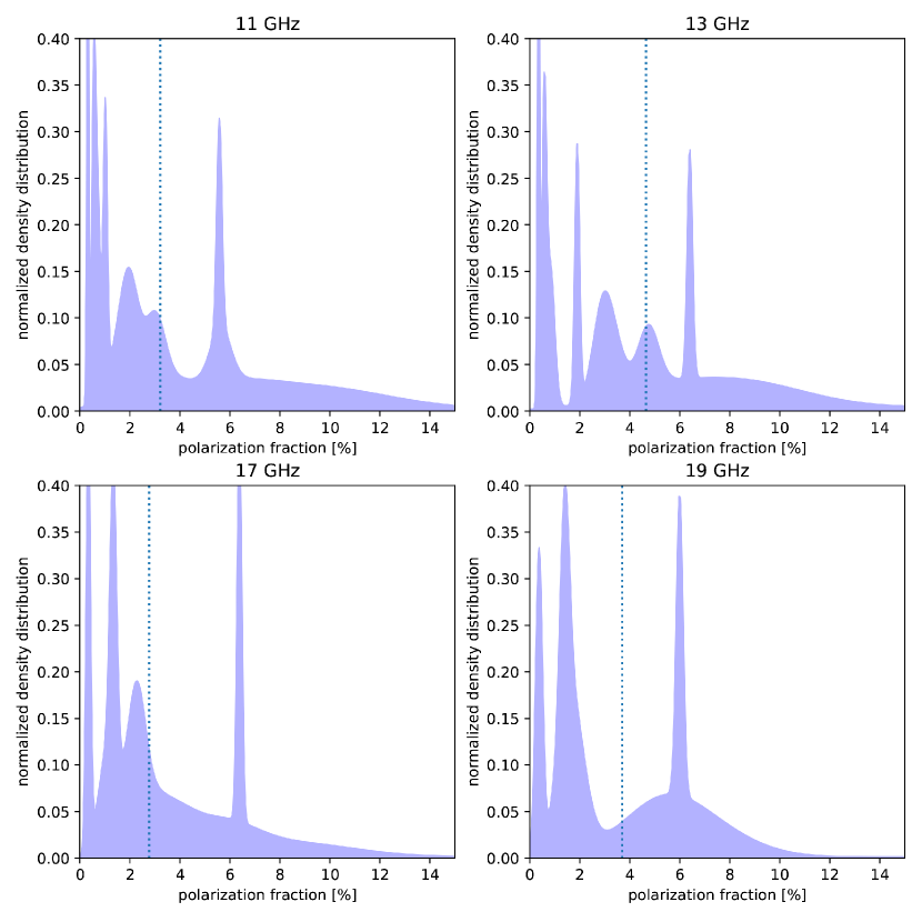
We have calculated the polarization fractions of the $99.99\%$ s.l. sources in our main sample (the 47 sources with polarization already measured by Planck). Figure 11 shows the density distribution of polarization fractions for these sources, assuming Gaussian uncertainties. Vertical lines indicate the median polarization fraction, which is $(3.2,4.7,2.8,3.7)\%$ at $(11,13,17,19)$ GHz. These median values have been computed from the cumulative density function (cdf) derived from the density distributions used for Figure 11. The advantage of using the density distributions instead of the discrete samples is that in this way it is possible easily to take into account the uncertainties in the estimation of the polarization fraction. The values obtained in this work are between median values reported in the literature for radio-flat sources (Sajina et al., 2011; Puglisi et al., 2018) and radio-steep sources (Murphy et al., 2010; Sajina et al., 2011; Puglisi et al., 2018) below $\nu<20$ GHz. The subsamples used for the calculation of the polarization fraction contain from $14\%$ at 13 GHz to $0\%$ at 17 and 19 GHz radio-steep sources. Table 6 shows the same median values and also the average value of the squared polarization fraction $\langle\Pi^{2}\rangle$. These values can be used in combination with the number counts to estimate the expected contribution from radio sources to the polarization power spectra of the QUIJOTE MFI data, as described in Lagache et al. (2020). The expected contribution is $\la 32,25,11,10$ $\mu$K.deg at 11, 13, 17 and 19 GHz respectively. These values are consistent with the predictions of Puglisi et al. (2018) and the best-fit results presented in Rubiño-Martín et al. (2023).

The same study for the extended sample gives significantly higher median polarization fractions: $\Pi_{\mathrm{med}}=(27.3,33.6,28.7,27.0)\%$ at $(11,13,17,19)$ GHz. The subsample of the extended catalogue used for the calculation of these polarization fractions is clearly dominated by steep sources (from a minimum value of $61\%$ steep sources found at 13 GHz to a maximum value of $85.7\%$ steep sources at 17 GHz). The high polarization fractions found for this subsample suggest that we may be overestimating the polarized flux density of the extended catalogue sources owing either to insufficient debiasing (equation 10) or to Eddington bias, even for high-significance sources.

6 Variability study

QUIJOTE-MFI data span a period of 6 yr, between November 2012 and August 2018, which allows for variability studies. These data have been separated in six different periods, with variable duration (2–22 months), which are calibrated independently (see Rubiño-Martín et al. (2023) and Génova-Santos et al. (2023) for details). The observations leading to the Wide Survey maps were taken during periods 1, 2, 5 and 6. Together with full-mission maps, maps per individual periods were also generated (see details in section 4.1.2 of Rubiño-Martín et al. (2023)). In order to identify variable sources (on time scales of $\gtrsim 6$ months), we have computed flux densities in total intensity for all sources having S/N $>5$ at 11 GHz in the four periods maps.

Flux densities extracted from maps of horns 2 and 4 are combined using appropriate weights (Rubiño-Martín et al., 2023) into one single measurement at both 16.8 GHz and 18.8 GHz. A correct estimate of the uncertainties associated with our flux density measurements is key to assessing variability. This estimate is based on error propagation from the scatter of the residuals of fits performed on individual-period maps from which we subtract the full map. We proceed in this way in order to eliminate the contribution from the sky background to the final error bar, which is common in all periods. Equally important is the estimate of the ‘effective observing date’. For each source we calculate this effective date as the weighted average of all the dates in which the source has been picked up by the telescope main beam (using the same weights that were used to weigh all the data lying in the same pixel when producing the final maps).

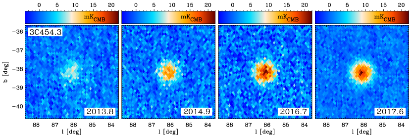
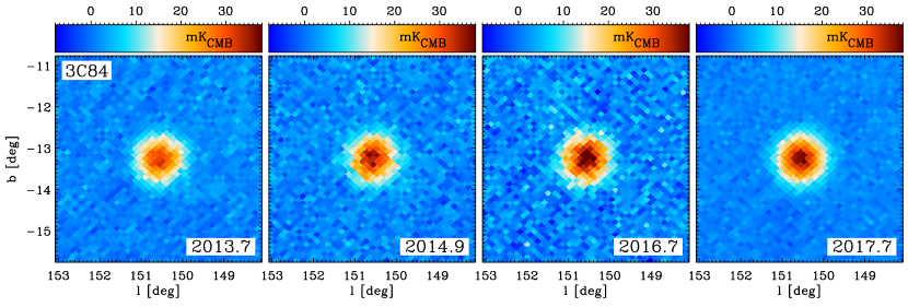
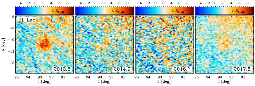
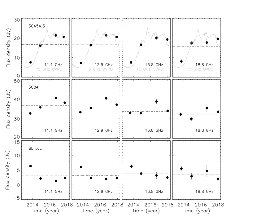
Figure 12 shows individual-period maps at $11.1$ GHz for three different sources. Variability can be seen by eye in these maps. It is also apparent that the map of period six is the most sensitive since it contains more data (22 months). For a better visualization of the variability trends, in Figure 13 we plot flux densities versus effective observing date for all four frequencies. Similar variability trends are observed for the four frequencies, despite the lower sensitivity of the two higher-frequency bands because of atmospheric contamination. It must be noted though that the noise in the two frequency pairs (11.1/12.9 GHz, and 16.8/18.8 GHz) is correlated to some extent, so those measurements cannot be considered as independent (although the lower- and higher-frequency measurements are). These variability trends are also similar to those traced by the 37 GHz data of the Metsähovi Radio Observatory.

Variability is assessed through a simple $\chi^{2}$ calculation to estimate the significance of the scatter of the 11 GHz flux densities (we use 11 GHz as a reference as it is the most sensitive band) over the four periods with respect to their weighted average (Chen et al., 2013). Table 7 shows the seven confirmed variable sources presenting the highest $\chi^{2}$. Note that the $\chi^{2}$ values at high frequencies are typically lower. This is a consequence of these data being noisier because they are more affected by atmospheric contamination. With three degrees of freedom, the $99\%$ confidence threshold is $\chi^{2}>11.3$, and all seven sources shown in Table 7 can therefore be considered as strongly variable (following the same criterion as Chen et al., 2013). These sources are the most compelling ones as they present similar variability trends in the four frequencies, which are also similar to the variability traced by the Metsähovi data. In total we detect 37 sources at 11.1 GHz with $\chi^{2}>11.3$. At lower confidence, we detect hints of variability consistent with Metsähovi in five other sources (4C39.25, PKS1502+106, 0642+449, 2201+315 and 0133+476). We have verified that sources that are found to be non-variable have $\chi^{2}$ per degree-of-freedom $\sim 1$, which bestows confidence on our error bar estimate.

This variability study has demonstrated the reliability of the internal gain calibration of the QUIJOTE-MFI Wide Survey data, whose accuracy is found to be better than $1\%$ (Rubiño-Martín et al., 2023; Génova-Santos et al., 2023). A more detailed and extended study of variability would entail binning the data on shorter timescales, which, even at the cost of less sensitivity may, reveal strongly variable sources over shorter periods. These and other studies (such as one on variability in polarization) will be presented in a future paper.

Figure 12: MFI maps at $11.1$ GHz per period (periods 1, 2, 5 and 6 from left to right) for three of the most variable sources identified in the survey: 3C454.3 (top), 3C84 (middle) and BL Lac (bottom). Effective observing date (in years) is shown in the bottom-right corner of each panel. For each source the colour scale of the maps has intentionally been normalized to the same values for all four periods. The change in the brightness of the source is appreciable by eye between the different periods.

Figure 13: Flux density as a function of time calculated on the individual-period maps at the four MFI frequencies (left to right) for three of the most variable sources (3C454.3, 3C84 and BL Lac). The horizontal dot-dashed lines depict densities extracted from the full map. For 3C454.3 we have overplotted the OVRO 15 GHz measurements.

$11.1$ GHz		$12.9$ GHz		$16.8$ GHz		$18.8$ GHz
Date	$S_{\nu}^{11}$ (Jy)	Date	$S_{\nu}^{13}$ (Jy)	Date	$S_{\nu}^{17}$ (Jy)	Date	$S_{\nu}^{19}$ (Jy)
3C454.3
2013.76	7.6$\pm$ 0.3	2013.77	7.2$\pm$ 0.3	2013.74	7.5$\pm$ 0.7	2013.73	8.1$\pm$ 0.9
2014.90	16.0$\pm$ 0.4	2014.91	16.3$\pm$ 0.4	2014.89	16.6$\pm$ 0.6	2014.91	17.4$\pm$ 1.1
2016.69	21.3$\pm$ 0.5	2016.69	21.3$\pm$ 0.5	2016.68	20.0$\pm$ 1.1	2016.68	17.7$\pm$ 1.6
2017.61	20.4$\pm$ 0.2	2017.90	20.5$\pm$ 0.2	2017.94	19.2$\pm$ 0.5	2017.95	19.5$\pm$ 0.7
$\chi^{2}$	1256		1520		205		102
3C84
2013.72	32.7$\pm$ 0.3	2013.70	33.3$\pm$ 0.3	2013.64	33.0$\pm$ 0.6	2013.65	32.2$\pm$ 0.9
2014.89	35.8$\pm$ 0.4	2014.91	35.4$\pm$ 0.4	2014.87	32.8$\pm$ 0.6	2014.89	29.9$\pm$ 1.0
2016.70	40.5$\pm$ 0.6	2016.69	40.4$\pm$ 0.5	2016.68	38.7$\pm$ 1.0	2016.68	35.4$\pm$ 1.7
2017.73	38.2$\pm$ 0.2	2017.91	37.2$\pm$ 0.2	2017.99	34.0$\pm$ 0.4	2017.99	33.6$\pm$ 0.6
$\chi^{2}$	352		216		27.1		12.9
Cas A
2013.80	356.6$\pm$ 0.4	2013.75	315.3$\pm$ 0.3	2013.83	249.0$\pm$ 1.0	2013.75	226.3$\pm$ 1.1
2014.90	350.5$\pm$ 0.8	2014.92	311.9$\pm$ 0.7	2014.88	250.4$\pm$ 0.5	2014.91	232.6$\pm$ 0.8
2016.70	350.4$\pm$ 0.4	2016.69	311.3$\pm$ 0.3	2016.67	251.2$\pm$ 0.9	2016.68	234.2$\pm$ 1.3
2017.94	348.8$\pm$ 0.3	2018.00	308.0$\pm$ 0.3	2018.11	243.3$\pm$ 0.7	2018.10	221.0$\pm$ 1.0
$\chi^{2}$	318		292		81.3		102
BL Lac
2013.76	6.4$\pm$ 0.3	2013.76	6.0$\pm$ 0.3	2013.78	6.2$\pm$ 0.6	2013.73	5.5$\pm$ 0.8
2014.93	2.1$\pm$ 0.4	2014.93	2.3$\pm$ 0.4	2014.90	3.8$\pm$ 0.6	2014.91	2.9$\pm$ 1.0
2016.71	1.2$\pm$ 0.5	2016.69	1.9$\pm$ 0.4	2016.68	3.2$\pm$ 1.0	2016.69	4.7$\pm$ 1.9
2017.77	2.3$\pm$ 0.2	2017.93	2.2$\pm$ 0.1	2017.95	2.5$\pm$ 0.4	2017.97	2.0$\pm$ 0.6
$\chi^{2}$	196		168		29.6		13.1
OJ287
2013.71	3.5$\pm$ 0.3	2013.67	3.7$\pm$ 0.3	2013.64	3.1$\pm$ 0.8	2013.64	2.1$\pm$ 1.9
2014.86	5.0$\pm$ 0.4	2014.89	5.2$\pm$ 0.4	2014.78	5.1$\pm$ 0.6	2014.85	4.1$\pm$ 1.2
2016.69	8.3$\pm$ 0.5	2016.70	7.7$\pm$ 0.6	2016.69	6.9$\pm$ 1.3	2016.69	5.7$\pm$ 2.0
2017.91	7.4$\pm$ 0.2	2017.98	8.0$\pm$ 0.2	2018.00	8.4$\pm$ 0.5	2018.00	8.5$\pm$ 0.7
$\chi^{2}$	127		137		40.6		18.1
Tau A
2013.63	454.0$\pm$ 0.6	2013.62	432.3$\pm$ 0.6	2013.54	391.3$\pm$ 1.0	2013.56	377.7$\pm$ 1.3
2014.88	451.5$\pm$ 0.9	2014.91	429.8$\pm$ 0.8	2014.86	380.8$\pm$ 0.9	2014.89	367.8$\pm$ 1.2
2016.70	450.4$\pm$ 0.7	2016.69	428.1$\pm$ 0.7	2016.69	386.9$\pm$ 1.4	2016.69	373.8$\pm$ 2.0
2017.84	449.6$\pm$ 0.4	2017.92	427.2$\pm$ 0.4	2018.09	384.1$\pm$ 0.6	2018.08	371.2$\pm$ 0.7
$\chi^{2}$	40.8		63.4		69.3		34.9
PKS1749+096
2013.77	3.5$\pm$ 0.3	2013.76	3.1$\pm$ 0.3	2013.85	2.2$\pm$ 0.6	2013.74	0.7$\pm$ 0.8
2014.90	5.0$\pm$ 0.4	2014.90	4.9$\pm$ 0.4	2014.87	4.2$\pm$ 0.6	2014.90	3.4$\pm$ 1.1
2016.69	3.4$\pm$ 0.5	2016.69	3.6$\pm$ 0.5	2016.70	3.8$\pm$ 1.2	2016.70	1.4$\pm$ 1.9
2017.67	2.2$\pm$ 0.2	2017.97	2.8$\pm$ 0.2	2018.04	3.2$\pm$ 0.3	2018.04	4.0$\pm$ 0.5
$\chi^{2}$	36.6		26.0		5.7		13.7

Table 7: Flux densities and effective observation dates of variable sources identified in the QUIJOTE-MFI survey. We show flux densities at the four MFI frequencies derived from maps of the four different periods, and the effective observation date (year). We also show $\chi^{2}$ values representing the scatter around the average value. The first three sources (3C454.3, 3C84, Cas A) are identified as strongly variable ($\chi^{2}>11.3$, with 3 degrees of freedom, corresponding to confidence $>99\%$). The other four, despite having a lower confidence, are known to be variable and show variability trends that are compatible with external datasets at similar frequencies.

7 Discussion and conclusions

In this paper, part of a series describing the data analysis and scientific results from the QUIJOTE MFI Wide Survey, we have studied 786 compact source candidates in the 11–19 GHz frequency range in both intensity and polarization. We have divided our sample into two catalogues: a main subsample containing 47 bright radio sources whose polarization has been measured by the Planck satellite (Planck Collaboration et al., 2016) and an extended subsample containing both 725 targets selected with flux density $\geq 1$ Jy at 30 GHz from the Second Planck Catalogue of Compact Sources (Planck Collaboration et al., 2016) and 14 additional SNR $\geq 4$ targets found by means of a blind search performed with the Mexican Hat Wavelet 2. In total, we have studied 786 targets which are being made public through the RADIOFOREGROUNDS web site.

The sources have been studied using a Python version of IFCAPOL, a software tool that implements a matched filter for the study of intensity and the Filtered Fusion (FF, Argüeso et al., 2009; López-Caniego et al., 2009) for the estimation of the polarimetric properties of the sources. For each of the targets we have estimated the (colour-corrected) I, Q and U Stokes parameters, the derived P and polarization angle measurements, and their associated uncertainties. We have also determined the statistical significance of the detection of the polarized signal as described in López-Caniego et al. (2009). For those sources with a clear detection, we have estimated the spectral index between 11 and 19 GHz (assuming a simple power-law emission) in both intensity and polarization.

We have performed a number of internal and external consistency tests. The internal consistency tests, using half-mission maps, have served to test both the stability of the instrument and the reliability of our photometry. We have also focused on three bright sources that have been used as calibrators (the Crab nebula, Cygnus A and Cassiopeia A) and checked that the photometry used in this paper is consistent with other photometric estimators (namely, aperture photometry and beam fitting) within the calibration uncertainty limit of the MFI maps. As an external consistency check, we have compared the photometry of 39 sources in our catalogues that have been observed during the same epoch with the VLA at $\sim$34 GHz. Though the comparison is difficult due to the frequency difference, the need to extrapolate using a simple power law, the difference in resolution and the variability of the sources, we find an overall good agreement between VLA and MFI observations. As an additional test, we have also studied the variability of a selected sample of sources in the MFI data and found it to be consistent with Metsähovi Radio Observatory observations.

We have also studied the statistical properties of our catalogue. A significant fraction of the sample is dominated by sources that are probably Galactic: 177 out of 786 (22.5%) sources have Galactic latitude $|b|\leq 10^{\circ}$. The number rises to 307 out of 786 (39.1%) if we allow $|b|\leq 20^{\circ}$. In spite of this, we have computed number counts (in total intensity only) with the sources that are likely to be extragalactic. Our results show good agreement with the De Zotti et al. (2005) model and suggest that our catalogue has a completeness limit at the $4.5\sigma$ level $\sim 1.8$ Jy at 11 GHz. We have also studied the distribution of colour-corrected spectral indexes in temperature for both Galactic and extragalactic sources. We find 15.2 per cent of steep sources outside the Galactic mask we have used, roughly consistent with the predictions of the De Zotti et al. (2005) model, but we must note that our statistics is very poor.

Finally, we have studied the polarimetric properties of (38, 33, 31, 23) sources with P detected with statistical significance $\geq 99.99\%$ at (11, 13, 17, 19) GHz respectively. MFI noise levels make it difficult to estimate the polarization angle of all but the brightest polarized sources. For this reason we do not attempt to extract information about the rotation measurement (RM) from this catalogue. For our main sample, we find median polarization fractions of $(3.2,4.7,2.8,3.7)\%$ at $(11,13,17,19)$ GHz. These values are between median values reported in the literature for radio flat sources (Sajina et al., 2011; Puglisi et al., 2018) and radio steep sources (Murphy et al., 2010; Sajina et al., 2011; Puglisi et al., 2018) below $\nu<20$ GHz. The median polarization fraction we find in our extended sample exceeds these values, which suggests that we may be overestimating the polarized flux density of the extended catalogue sources.

Data availability

All data products can be freely downloaded from the QUIJOTE web, as well as from the RADIOFOREGROUNDS platform. They include also an Explanatory Supplement describing the data formats. Maps will be submitted also to the Planck Legacy Archive (PLA) interface and the LAMBDA site. Any other derived data products described in this paper (half-survey maps, simulations, etc.) are available upon request to the QUIJOTE collaboration.

References

- AMI Consortium et al. (2011) AMI Consortium et al., 2011, MNRAS, 415, 2699
- Argüeso et al. (2009) Argüeso F., Sanz J. L., Herranz D., López-Caniego M., González-Nuevo J., 2009, MNRAS, 395, 649
- Astropy Collaboration et al. (2013) Astropy Collaboration et al., 2013, A&A, 558, A33
- Astropy Collaboration et al. (2018) Astropy Collaboration et al., 2018, AJ, 156, 123
- Battye et al. (2011) Battye R. A., Browne I. W. A., Peel M. W., Jackson N. J., Dickinson C., 2011, MNRAS, 413, 132
- Bennett & Simth (1962) Bennett A. S., Simth F. G., 1962, Monthly Notices of the Royal Astronomical Society, 125, 75
- Bennett et al. (2013) Bennett C. L., et al., 2013, ApJS, 208, 20
- Bonavera et al. (2017) Bonavera L., González-Nuevo J., Argüeso F., Toffolatti L., 2017, MNRAS, 469, 2401
- Chen et al. (2013) Chen X., Rachen J. P., López-Caniego M., Dickinson C., Pearson T. J., Fuhrmann L., Krichbaum T. P., Partridge B., 2013, A&A, 553, A107
- Datta et al. (2019) Datta R., et al., 2019, MNRAS, 486, 5239
- De Zotti et al. (2005) De Zotti G., Ricci R., Mesa D., Silva L., Mazzotta P., Toffolatti L., González-Nuevo J., 2005, A&A, 431, 893
- De Zotti et al. (2010) De Zotti G., Massardi M., Negrello M., Wall J., 2010, A&ARv, 18, 1
- De Zotti et al. (2019) De Zotti G., et al., 2019, Bulletin of the AAS, 51
- Foreman-Mackey et al. (2013) Foreman-Mackey D., Hogg D. W., Lang D., Goodman J., 2013, PASP, 125, 306
- Galluzzi & Massardi (2016) Galluzzi V., Massardi M., 2016, International Journal of Modern Physics D, 25, 1640005
- Galluzzi et al. (2018) Galluzzi V., et al., 2018, MNRAS, 475, 1306
- Gawroński et al. (2010) Gawroński M. P., et al., 2010, MNRAS, 406, 1853
- Génova-Santos et al. (2023) Génova-Santos R. T., Rubiño-Martín J. A., et al., 2023, MNRAS, in prep.
- Gómez-Reñasco et al. (2012) Gómez-Reñasco M. F., et al., 2012, in Millimeter, Submillimeter, and Far-Infrared Detectors and Instrumentation for Astronomy VI. p. 845234, doi:10.1117/12.926416
- González-Nuevo et al. (2006) González-Nuevo J., Argüeso F., López-Caniego M., Toffolatti L., Sanz J. L., Vielva P., Herranz D., 2006, MNRAS, 369, 1603
- González-Nuevo et al. (2008) González-Nuevo J., Massardi M., Argüeso F., Herranz D., Toffolatti L., Sanz J. L., López-Caniego M., De Zotti G., 2008, MNRAS, 384, 711
- Górski et al. (2005) Górski K. M., Hivon E., Banday A. J., Wandelt B. D., Hansen F. K., Reinecke M., Bartelmann M., 2005, ApJ, 622, 759
- Gregory et al. (1996) Gregory P. C., Scott W. K., Douglas K., Condon J. J., 1996, Astrophys. J. Suppl., 103, 427
- Guidi et al. (2021) Guidi F., et al., 2021, MNRAS, 507, 3707
- Harris et al. (2020) Harris C. R., et al., 2020, Nature, 585, 357–362
- Healey et al. (2007) Healey S. E., Romani R. W., Taylor G. B., Sadler E. M., Ricci R., Murphy T., Ulvestad J. S., Winn J. N., 2007, ApJS, 171, 61
- Herranz & Vielva (2010) Herranz D., Vielva P., 2010, IEEE Signal Processing Magazine, 27, 67
- Hoyland et al. (2012) Hoyland R. J., et al., 2012, in Millimeter, Submillimeter, and Far-Infrared Detectors and Instrumentation for Astronomy VI. p. 845233, doi:10.1117/12.925349
- Huffenberger et al. (2015) Huffenberger K. M., et al., 2015, The Astrophysical Journal, 806, 112
- Hunter (2007) Hunter J. D., 2007, Computing in Science Engineering, 9, 90
- Jackson et al. (2010) Jackson N., Browne I. W. A., A. B. R., D. G., Taylor A. C., 2010, MNRAS, 401, 1388
- Kamionkowski et al. (1997) Kamionkowski M., Kosowsky A., Stebbins A., 1997, Physical Review D, 55, 7368
- Kay (1998) Kay S. M., 1998, Fundamentals of Statistical Signal Processing, Volume 2: Detection Theory. Prentice Hall PTR, http://www.worldcat.org/isbn/013504135X
- Lagache et al. (2020) Lagache G., M. B., Montier L., Serra P., Tucci M., 2020, Astronomy and Astrophysics, 642, A232
- López-Caniego et al. (2006) López-Caniego M., Herranz D., González-Nuevo J., Sanz J. L., Barreiro R. B., Vielva P., Argüeso F., Toffolatti L., 2006, MNRAS, 370, 2047
- López-Caniego et al. (2007) López-Caniego M., González-Nuevo J., Herranz D., Massardi M., Sanz J. L., De Zotti G., Toffolatti L., Argüeso F., 2007, ApJS, 170, 108
- López-Caniego et al. (2009) López-Caniego M., Massardi M., González-Nuevo J., Lanz L., Herranz D., De Zotti G., Sanz J. L., Argüeso F., 2009, ApJ, 705, 868
- Lopez-Caraballo et al. (2023) Lopez-Caraballo C. H., et al., 2023, MNRAS, in prep.
- Massardi et al. (2009) Massardi M., López-Caniego M., González-Nuevo J., Herranz D., De Zotti G., Sanz J. L., 2009, MNRAS, 392, 733
- Montier et al. (2015) Montier L., Plaszczynski S., Levrier F., Tristram M., Alina D., Ristorcelli I., Bernard J. P., 2015, A&A, 574, A135
- Murphy et al. (2010) Murphy T., et al., 2010, MNRAS, 402, 2403
- Peel et al. (2022) Peel M. W., Genova-Santos R., Dickinson C., Leahy J. P., López-Caraballo C., Fernández-Torreiro M., Rubiño-Martín J. A., Spencer L. D., 2022, Research Notes of the American Astronomical Society, 6, 252
- Pérez-de-Taoro et al. (2016) Pérez-de-Taoro M. R., et al., 2016, in Ground-based and Airborne Telescopes VI. p. 99061K, doi:10.1117/12.2233225
- Perrott et al. (2021) Perrott Y. C., et al., 2021, MNRAS, submitted
- Planck Collaboration ES (2018) Planck Collaboration ES 2018, The Legacy Explanatory Supplement, https://wiki.cosmos.esa.int. ESA
- Planck Collaboration et al. (2011) Planck Collaboration et al., 2011, A&A, 536, A7
- Planck Collaboration et al. (2014) Planck Collaboration et al., 2014, A&A, 571, A28
- Planck Collaboration et al. (2016) Planck Collaboration et al., 2016, A&A, 594, A26
- Planck Collaboration et al. (2018) Planck Collaboration et al., 2018, A&A, 619, A94
- Puglisi et al. (2018) Puglisi G., et al., 2018, ApJ, 858, 85
- Richards et al. (2011) Richards J. L., et al., 2011, ApJS, 194, 29
- Rubiño-Martín et al. (2010) Rubiño-Martín J. A., et al., 2010, Astrophysics and Space Science Proceedings, 14, 127
- Rubiño-Martín et al. (2012) Rubiño-Martín J. A., et al., 2012, in Ground-based and Airborne Telescopes IV. p. 84442Y, doi:10.1117/12.926581
- Rubiño-Martín et al. (2023) Rubiño-Martín J. A., Guidi F., Génova Santos R. T., et al., 2023, MNRAS, accepted
- Sajina et al. (2011) Sajina A., Partridge B., Evans T., Stefl S., Vechik N., Myers S., Dicker S., Korngut P., 2011, ApJ, 732, 45
- Seljak & Hirata (2004) Seljak U., Hirata C. M., 2004, Phys. Rev. D, 69, 043005
- Tucci & Toffolatti (2012) Tucci M., Toffolatti L., 2012, Advances in Astronomy, 2012, 624987
- Tucci et al. (2005) Tucci M., Martínez-González E., Vielva P., Delabrouille J., 2005, MNRAS, 360, 935
- Tucci et al. (2011) Tucci M., Toffolatti L., De Zotti G., Martínez-González E., 2011, A&A, 533, A57
- Virtanen et al. (2020) Virtanen P., et al., 2020, Nature Methods, 17, 261
- Wright et al. (1994) Wright A. E., Griffith M. R., Burke B. F., Ekers R. D., 1994, ApJS, 91, 111
- Zonca et al. (2019) Zonca A., Singer L., Lenz D., Reinecke M., Rosset C., Hivon E., Gorski K., 2019, Journal of Open Source Software, 4, 1298