QUIJOTE Scientific Results – VII. Galactic AME sources in the QUIJOTE-MFI Northern Hemisphere Wide-Survey

Abstract

The QUIJOTE-MFI Northern Hemisphere Wide-Survey has provided maps of the sky above declinations $-30^{\circ}$ at 11, 13, 17 and 19 GHz. These data are combined with ancillary data to produce Spectral Energy Distributions in intensity in the frequency range 0.4–3 000 GHz on a sample of 52 candidate compact sources harbouring anomalous microwave emission (AME). We apply a component separation analysis at 1^∘ scale on the full sample from which we identify 44 sources with high AME significance. We explore correlations between different fitted parameters on this last sample. QUIJOTE-MFI data contribute to notably improve the characterisation of the AME spectrum, and its separation from the other components. In particular, ignoring the 10–20 GHz data produces on average an underestimation of the AME amplitude, and an overestimation of the free-free component. We find an average AME peak frequency of 23.6 $\pm$ 3.6 GHz, about 4 GHz lower than the value reported in previous studies. The strongest correlation is found between the peak flux density of the thermal dust and of the AME component. A mild correlation is found between the AME emissivity ($A_{\rm AME}/\tau_{250}$) and the interstellar radiation field. On the other hand no correlation is found between the AME emissivity and the free-free radiation Emission Measure. Our statistical results suggest that the interstellar radiation field could still be the main driver of the intensity of the AME as regards spinning dust excitation mechanisms. On the other hand, it is not clear whether spinning dust would be most likely associated with cold phases of the interstellar medium rather than with hot phases dominated by free-free radiation.

1 Introduction

A detailed knowledge of the sky emission properties in the frequency range $\sim$1–3 000 GHz, from low-frequency (LF) bands at which the Galactic synchrotron emission generally dominates, to high frequency (HF) bands at which the Galactic dust emission dominates, is crucial for a state-of-the art characterization of the Cosmic Microwave Background (CMB) radiation both in intensity and in polarization (e.g. Planck Collaboration et al., 2020; LiteBIRD Collaboration et al., 2022). Understanding the properties of the Galactic foregrounds is essential in order to measure a possibly intrinsic polarization signature in the CMB emission that could give insights about inflation scenarios. This task is considered to be a serious challenge by both the community of astronomers in quest of a B-mode detection (see Watts et al., 2015; POLARBEAR Collaboration et al., 2017; The Simons Observatory Collaboration et al., 2019; Aiola et al., 2020; The CMB-S4 Collaboration et al., 2022; Planck Collaboration et al., 2020; BICEP/Keck collaboration et al., 2021; The LSPE collaboration et al., 2021; Lee et al., 2021; LiteBIRD Collaboration et al., 2022; Hamilton et al., 2022) and the community of astronomers interested to understand the spatial and spectral variations of the Galactic emission (see Jones et al., 2018; Carretti et al., 2019; Rubiño-Martín et al., 2023).

In addition to synchrotron emission and thermal dust emission, the Galactic sky also emits thermal bremmstrahlung or free-free radiation, a radiation produced by deceleration of electrons, and supposedly unpolarized (Rybicki & Lightman, 1979; Trujillo-Bueno et al., 2002). Another type of radiation is the so-called Anomalous Microwave Emission (AME) that was discovered about twenty five years ago (see Leitch et al., 1997; Kogut, 1997; de Oliveira-Costa et al., 1998). The AME is a diffuse component showing a spectral bump detected over almost the full sky in the frequency range 10–60 GHz and peaking in flux density around a central frequency of $\sim$ 30 GHz. In this frequency range, the synchrotron and free-free emission can dominate over the AME emission while the thermal dust emission is expected to be negligible. The carriers and physical mechanisms producing AME are not conclusively known yet, however theoretical emission mechanisms have been proposed based on phenomenological interpretations of correlations found between the AME radiation and other Galactic template components. A review of these aspects and of the proposed models in the literature is given by Dickinson et al. (2018). The main current paradigm is that electric dipole emission from very small fast rotating spinning dust grains out of thermal equilibrium could be the origin of this emission (see Draine & Lazarian, 1998; Ali-Haïmoud et al., 2009; Hoang et al., 2010; Ysard & Verstraete, 2010). Recent advances on the development of another model, initially proposed by Jones (2009) and exploring the possibility that AME can be produced instead by thermal amorphous dust are discussed by Nashimoto et al. (2020a) and Nashimoto et al. (2020b). The majority of these models predict very low levels of polarisation for the AME, this being supported by observational data (López-Caraballo et al., 2011; Dickinson et al., 2011; Rubiño-Martín et al., 2012a; Génova-Santos et al., 2017).

Given its twofold role as a CMB contaminant and as a source of information about the physics of the ISM, it is important to make progress on the study of the observational properties of AME, and confronting them with theoretical models. Galactic candidate AME sources were intensively discussed in Planck Collaboration et al. (2014a) (herefater PIRXV). In that work the analysis of a sample of 98 compact candidate AME sources distributed over the full sky provides significant detection ($>5\sigma$) of AME for 42 sources, which reduces to safe detection of AME for 27 sources once the potential contribution of thick free-free emission from ultra compact H ii regions has been integrated to the analysis. In this work, we complete and revisit the sample of sources observable from the Northern hemisphere. For this we use the QUIJOTE-MFI wide-survey maps (Rubiño-Martín et al., 2023), which are crucial to pin down the AME spectrum at low frequencies, thence allowing a more reliable separation between the AME and free-free amplitudes (e.g., Poidevin et al., 2019) than previous works, which systematically have overestimated the free-free emission and underestimated the AME amplitude. Some of the sections in the present article closely follow those in PIRXV. In such cases we tried to use similar section names so that the reader can easily refer to the information provided by PIRXV and, as much as possible, we tried to avoid redundancy with their explanations. All the calculations made for our analysis are independent of those done by PIRXV.

The structure of the article is as follows: the data used for the analysis are presented in Section 2. The sample selection and fitting procedure used for the Spectral Energy Distribution (SED) analysis are detailed in Section 3. Consistency checks obtained from the comparison of our method with that used by PIRXV are also presented in that Section. The significance of the AME detection obtained from our analysis, potential contamination by UCH ii regions and robustness and validation of our method are discussed in Section 4. Statistics on the parameters characterizing the sample of regions that passed the validation tests are investigated in Section 5. A discussion is given in Section 6. Our results and conclusions are summarized in Section 7. Additional plots showing low Spearman rank correlation coefficients (SRCCs) between some of the parameters obtained from the modelling of the SEDs, and mentioned in some of the above sections, are presented in Appendix A. All the parameters estimates obtained from the modelling of the SEDs, and additional information, obtained on the full sample, are tabulated in Appendix B. All the plots of the SEDs and the multicomponents models are shown in Appendix C. Finally, a summary of the SRCCs obtained between all the pairs of parameters used to model the SEDs are given in Appendix D.

2 Data

The maps used in this analysis are listed in Table 1. Details about the maps are given in the following subsections.

Frequency	Wavelength	Telescope$/$	Angular Resolution	Original	Calibration	References
[GHz]	[mm]	survey	[′]	Units	Uncertaintiy [$\%$]
0.408	735.42	JB$/$Eff$/$Parkes	$\approx$ 60	[KRJ]	10	Haslam et al. (1982)
						Remazeilles et al. (2015)
0.820	365.91	Dwingeloo	72	[KRJ]	10	Berkhuijsen (1972)
1.420	211.30	Stockert/Villa-Elisa	36	[KRJ]	10	Reich (1982)
						Reich & Reich (1986)
						Reich et al. (2001)
11.1	28.19	QUIJOTE	55.4	[mKCMB]	5	Rubiño-Martín et al. (2023)
12.9	23.85	QUIJOTE	55.8	[mKCMB]	5	Rubiño-Martín et al. (2023)
16.8	18.24	QUIJOTE	38.9	[mKCMB]	5	Rubiño-Martín et al. (2023)
18.8	16.32	QUIJOTE	40.3	[mKCMB]	5	Rubiño-Martín et al. (2023)
22.8	13.16	WMAP 9-yr	$\approx$ 49	[mKCMB]	3	Bennett et al. (2013)
28.4	10.53	$Planck$ LFI	$32.29$	[KCMB]	3	Planck Collaboration et al. (2016a)
33.0	9.09	WMAP 9-yr	$\approx 40$	[mKCMB]	3	Bennett et al. (2013)
40.6	7.37	WMAP 9-yr	$\approx 31$	[mKCMB]	3	Bennett et al. (2013)
44.1	6.80	$Planck$ LFI	$27$	[KCMB]	3	Planck Collaboration et al. (2016a)
60.8	4.94	WMAP 9-yr	$\approx 21$	[mKCMB]	3	Bennett et al. (2013)
70.4	4.27	$Planck$ LFI	$13.21$	[KCMB]	3	Planck Collaboration et al. (2016a)
93.5	3.21	WMAP 9-yr	$\approx 13$	[mKCMB]	3	Bennett et al. (2013)
100	3.00	$Planck$ HFI	$9.68$	[KCMB]	3	Planck Collaboration et al. (2016a)
143	2.10	$Planck$ HFI	$7.30$	[KCMB]	3	Planck Collaboration et al. (2016a)
217	1.38	$Planck$ HFI	$5.02$	[KCMB]	3	Planck Collaboration et al. (2016a)
353	0.85	$Planck$ HFI	$4.94$	[KCMB]	3	Planck Collaboration et al. (2016a)
545	0.55	$Planck$ HFI	$4.83$	[MJy/sr]	6.1	Planck Collaboration et al. (2016a)
857	0.35	$Planck$ HFI	$4.64$	[MJy/sr]	6.4	Planck Collaboration et al. (2016a)
1249	0.24	COBE-DIRBE	$\approx 40$	[MJy/sr]	11.9	Hauser et al. (1998)
2141	0.14	COBE-DIRBE	$\approx 40$	[MJy/sr]	11.9	Hauser et al. (1998)
2998	0.10	COBE-DIRBE	$\approx 40$	[MJy/sr]	11.9	Hauser et al. (1998)

Table 1: List of surveys and maps used in our analysis.

2.1 QUIJOTE Data

The data used at frequencies 11, 13, 17 and 19 GHz come from the first release of the QUIJOTE wide survey maps (Rubiño-Martín et al., 2023). These maps were obtained from $9\,200$ h of data collected over 6 years of observations from 2012 to 2018 with the Multi-Frequency Instrument (MFI) on the first QUIJOTE telescope, from the Teide Observatory in Tenerife, Canary Islands, Spain at an altitude of $2\,400$ meters above sea level, at 28.3^∘ N and 16.5^∘ W. These observations were performed at constant elevations and with the telescope continuously spinning around the azimuth axis (the so-called “nominal mode”) to obtain daily maps of the full northern sky. After combination of all these data we obtained maps covering $\sim 70\%$ of the sky and with sensitivities in total intensity between 60 and 200 $\mu$K/deg, depending on the horn and frequency and sensitivites, down to $\sim 35\mu$K/deg, in polarisation. Full details on these maps, and multiple characterisation and validation tests, are given in Rubiño-Martín et al. (2023), while the general MFI data processing pipeline will be described in Génova-Santos et al. (2023).

The MFI consists of 4 horns, two of them (horns 1 and 3) covering a 10-14 GHz band with two outputs channels centred at 11 and 13 GHz, and two other ones (horns 2 and 4) covering the 16-20 GHz band with two output channels at 17 and 19 GHz (Génova-Santos et al., 2023). Due to a malfunctioning of horn 1 in polarization during some periods, all the scientific QUIJOTE papers associated with this release make use of horn 3 only at 11 and 13 GHz. Although this paper uses intensity data only, we follow the same criterion and use only horn 3, which is much better characterised. At 17 and 19 GHz we combine data from horns 2 and 4 through a weighted mean, using predefined constant weights (Rubiño-Martín et al., 2023). Finally, it must be noted that, due to the use of the same low-noise amplifiers, the noises from the lower and upper frequency bands of each horn are significantly correlated (see Section 4.3.3 in Rubiño-Martín et al., 2023). In principle this correlation should be accounted for in any scientific analysis that uses spectral information. However, we have checked that neglecting them introduces a small effect on the results presented in this paper. AME parameters are the most affected, and we have checked that accounting for this correlation introduces differences in these parameters that are typically below the 3% level. Therefore, for the sake of simplicity we decided to use the four frequency points (nominal frequencies 11.1, 12.9, 16.8 and 18.8 GHz) in the analysis as independent data points. We assume a 5% overall calibration uncertainty of the QUIJOTE MFI data, which is added in quadrature to the statistical error bar. There is compelling evidence that this $5\,\%$ value, which is driven by uncertainties in the calibration models, is sufficiently conservative (Génova-Santos et al., 2023; Rubiño-Martín et al., 2023).

2.2 Ancillary Data

2.2.1 Low frequency ancillary data

At low frequencies we use a destriped version (Platania et al., 2003) of the all-sky 408 MHz map of Haslam et al. (1982), the Dwingeloo survey map at 0.820 GHz of Berkhuijsen (1972), and the 1.420 GHz map of Reich (1982). Since our study is focused on compact candidate AME sources we prefer to use the all-sky 408 MHz destriped map of Haslam et al. (1982). The Platania et al. (2003) version of this map is used for consistency with previous QUIJOTE papers, but we have checked that the results are consistent with those obtained using the map provided by Remazeilles et al. (2015). The Jonas et al. (1998) map at 2.326 GHz, which was used in PIRXV, measures $I+Q$. Therefore it would lead to residuals in polarised regions, and we prefer not to use it.

Some of the considered sources are not well sampled or not included in the footprint of some of the ancillary maps. Therefore, for a given source a map is used only if all pixels within a circular region of $3^{\circ}$ radius are covered. We noted that, for a subset of compact sources, the map at 1.420 GHz shows a misscentering of the emission by more than half a degree with respect to other low-frequency maps. For that reason we prefer not to use that map in the analysis of G$059.42-00.21$, G$061.47+00.11$ and G$099.60+03.70$. The 1.420 GHz map is calibrated to the full beam, and therefore we apply the full-beam to main-beam recalibration factor of 1.55 for compact sources derived by Reich & Reich (1988). Overall, we assume a 10$\,\%$ uncertainty in the radio data at low frequency, which encompasses intrinsic calibration uncertainties as well as issues related with beam uncertainties and recalibration factors.

2.2.2 WMAP Maps

At frequencies of 23, 33, 41, 61, and 94 GHz, we use the intensity maps from the 9-year data release of the WMAP satellite (Bennett et al., 2013). All the maps were retrieved from the LAMBDA database. For all the maps we assume a 3$\%$ overall calibration uncertainty. The uncertainty in WMAP’s amplitude calibration is much better, however here we use 3$\%$ to account for other systematic effects like uncertainties in the beams or bandpasses (which in turn lead to uncertainties in the colour corrections) that will have a direct effect on our derived flux densities.

2.2.3 Planck Maps

Below 100 GHz intensity maps are available at frequencies 28, 44, and 70 GHz. They were obtained with the Low-Frequency Instrument (LFI) on board of the Planck satellite (Planck Collaboration et al., 2016a). We use the second public release version of the intensity maps as provided by the Planck Legacy Archive (PLA). Above 100 GHz we use the second data release version of the intensity maps obtained with the High-Frequency Instrument (HFI) on board the Planck satellite (Planck Collaboration et al., 2016a) at frequencies centred at 100, 143, 217, 353, 545, and 857 GHz. We have checked that using the third data release (PR3) leads to differences in the derived flux densities typically below $0.3\,\%$ for most of the frequencies and therefore have no impact in the final results presented in this paper. The Type 1 CO maps (Planck Collaboration et al., 2014b) were used to correct the 100, 217, and 353 GHz intensity maps for contamination introduced by the CO rotational transition lines (1-0), (2-1) and (3-2), respectively. We assume an overall calibration uncertainty of 3 $\%$ for the LFI data, and also for the HFI data at frequencies lower than or equal to 353 GHz, a value of 6.1$\%$ at 545 GHz, and a value of 6.4$\%$ at 857 GHz (Planck Collaboration et al., 2016b).

2.2.4 High frequency ancillary data

In the FIR range we use the Zodi-Subtracted Mission Average (ZSMA) COBE-DIRBE maps (Hauser et al., 1998) at 240 $\mu$m (1249 GHz), 140$\,\mu$m (2141 GHz), and 100$\,\mu$m (2997 GHz). We assume an 11.9$\%$ overall calibration uncertainty in the data at these frequencies.

3 Sample selection and SED fitting

In the following section we describe the process followed to build the sample of the candidate compact Galactic AME sources. Details about aperture photometry used to build the SEDs are given in Section 3.2. The modelling used to analyse the SED of each candidate AME source is detailed in Section 3.3. Finally, a consistency test is investigated and a comparison of our analysis, including the QUIJOTE maps, with the analysis obtained by Planck Collaboration et al. (2014a) on the sample of sources common to both studies is given in Section 3.4.

Source Name	Glon	Glat	Region Type	Other Name(a)	References	$\sigma_{\rm AME}$	$\sigma_{\rm AME}$
	$[^{\circ}]$	$[^{\circ}]$				PIRXV	This Work
G010.19$-$00.32	10.19	$-$0.32	SNR	Kes62. Synch. SNR9.9$-$0.8	1	3.4S	2.6SS
G010.84$-$02.59	10.84	$-$2.59	MC	GGD 27	2	…	4.8SS
G011.11$-$00.12	10.60	$-$0.12	MC	G011.11$-$0.12	2	…	2.5SS
G012.80$-$00.19	12.80	$-$0.19	SNR	W33	1	2.7	1.2LD
G015.06$-$00.69	15.06	$-$0.69	MC	M17	1	1.9	8.0S→SS
G017.00+00.85	17.00	0.85	MC	M16	1,2	5.3	6.0S
G037.79$-$00.11	37.79	$-$0.11	SNR	W47	1	3.4	7.6S→SS
G040.52+02.53	40.52	2.53	MC/HII	W45	1	0.2	12.9S→SS
G041.03$-$00.07	41.03	$-$0.07	MC	SDC G41.003$-$0.097	4	…	7.9S
G043.20$-$00.10	43.20	$-$0.10	MC	W49	1,3	5.3	8.3S→SS
G045.47+00.06	45.47	0.06	SNR	NRAO601	1	5.9	15.6S→SS
G049.14$-$00.60	49.14	$-$0.60	MC/HII	W51	2	…	22.9S→SS
G059.42$-$00.21	59.42	$-$0.21	MC/HII	W55	1	7.0	8.7S→SS
G061.47+00.11	61.47	0.11	MC/HII	HII LBN061.50+00.29. SH2$-$88	1	1.9	4.1SS
G062.98+00.05	62.98	0.05	MC	S89	1	7.5	6.1S→SS
G070.14+01.61	70.14	1.61	Cluster	NGC 6857	4	…	3.1BD
G071.59+02.85	71.59	2.85	MC/HII	s101	1	1.8	4.8SS
G075.81+00.39	75.81	0.39	MC/HII	HII GAL075.84+00.40. SH2$-$105. Cyg 2N	1	2.5	5.9S→SS
G076.38$-$00.62	76.38	$-$0.62	MC/HII	S106	1,3	…	3.9BD
G078.57+01.00	78.57	1.00	MC/HII	LDN 889	2,3	…	…BD
G081.59+00.01	81.59	0.01	MC/HII	DR23/DR21	1,2	1.3	17.9S
G084.68$-$00.58	84.68	$-$0.58	MC	DOBASHI 2732	4	…	18.8S
G085.00+04.20	84.90	3.80	MC/HII	LBN 084.97+04.21	4	…	21.1S
G093.02+02.76	93.02	2.76	MC/HII	HII GAL093.06+2.81	1	1.6	21.0S→SS
G094.47$-$01.53	94.47	$-$1.53	MC/HII	LDN 1059	1	0.6	4.1SS
G098.00+01.47	98.00	1.47	MC/HII	RNe GM1-12, DNe TGU H582	1	6.1	17.2S→SS
G099.60+03.70	99.60	3.70	MC	LDN1111	1	0.6	3.0SS
G102.88$-$00.69	102.88	$-$0.69	MC/HII	LDN1161/1163	1	2.5	10.9S
G107.20+05.20	107.20	5.20	MC	S140	1,2	9.9	27.8S→SS
G110.25+02.58	110.25	2.58	MC/HII	HII G110.2+02.5. LBN110.11+02.44	1	3.4	2.7SS
G111.54+00.81	111.54	0.81	Open Cluster	NGC 7538	2	…	10.8S→SS
G118.09+04.96	118.09	4.96	SNR	NGC 7822	1	…	14.2S
G123.13$-$06.27	123.13	$-$6.27	MC/HII	S184	2	…	25.2S→SS
G133.27+09.05	133.27	9.05	MC	LDN 1358/1355/1357	1	8.5S	11.1BD
G133.74+01.22	133.74	1.22	MC	W3	1	1.5	24.8S→SS
G142.35+01.35	142.35	1.35	MC	DNe TGU H942, DOBASHI 3984	1	9.5S	8.4S
G151.62$-$00.28	151.62	$-$0.28	MC/HII	HII SH2$-$209	1	1.5	11.4S→SS
G160.26-18.62	160.26	$-$18.62	MC	Perseus	1,2	17.4S	19.2S
G160.60$-$12.05	160.60	$-$12.05	MC	NGC 1499 (California nebula)	1	5.1S	12.6S
G173.56$-$01.76	173.56	$-$1.76	Open Cluster	NGC 1893	1	0.8	4.4SS
G173.62+02.79	173.62	2.79	Cluster	S235	1	5.6	15.5S→SS
G190.00+00.46	190.00	0.46	MC/HII	NGC 2174/2175	1	7.4	29.3S→SS
G192.34$-$11.37	192.34	$-$11.37	MC	LDN 1582/1584	1	12.3S	12.5BD
G192.60$-$00.06	192.60	$-$0.06	Cluster	S255	1	4.3	7.9S→SS
G201.62+01.63	201.62	1.63	MC	LDN 1608/1609	1	7.4S	27.3S
G203.24+02.08	203.24	2.08	MC/HII	LDN 1613	1,2	8.3S	15.8S
G208.80$-$02.65	208.80	$-$2.65	MC/HII	S280–LBN 970	1	2.0	1.9LD
G239.40$-$04.70	239.40	$-$4.70	MC	LDN 1667, HII LBN1059, V VY Cma	1	9.9S	16.5S
G351.31+17.28	351.31	17.28	MC/HII	HII LBN1105/1104	1	5.3S	32.9S
G353.05+16.90	353.05	16.90	MC	Rho Ophiuchi, AME-G353.05+16.901	1,3	29.8S	27.3S→SS
G353.97+15.79	353.97	15.79	MC	In Ophiuchus	1	10.9S	10.6S
G355.63+20.52	355.63	20.52	MC	In Rho Ophiuchus	1	13.3S	17.0BD

Table 2: List of sources. References: 1: Planck Collaboration et al. (2014a) (PIRXV), 2: Matthews et al. (2009), 3: Crutcher (1999), 4: Lee et al. (2016). Note: ^(a) information retrieved from the Simbad database (http://simbad.u-strasbg.fr/simbad//). Sources such that $\sigma_{\rm AME}$ from PIRXV are greater than $\sigma_{\rm AME}$ from this work are shown in bold. Superscript symbols in last two columns are ^S for “significant” AME detection, ^SS for “semi-significant” AME detection, ^S→SS for “significant” AME detection reclassified as “semi-significant” AME detection (see text for details), ^LD for low detection of AME and, ^BD for bad detection because of a bad fit of the AME, of the free-free or of the thermal dust component. See section 4.3 for details.

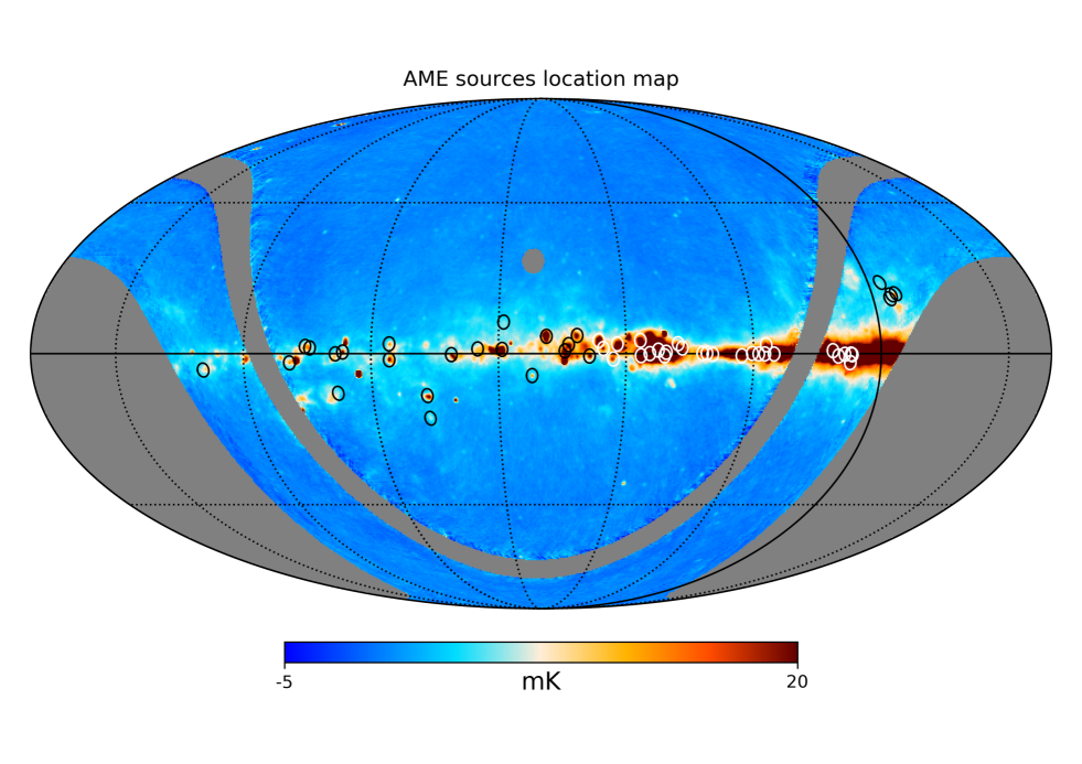
Figure 1: AME sources location in the Galaxy displayed on top of the QUIJOTE-MFI 11 GHz wide survey map at 1 degree resolution. Coordinates are listed in Table 2. The map is centred at position $(l,b)=(120^{\circ},0^{\circ})$.

3.1 AME sources sample

To build the sample of candidate AME sources, we use the list of sources selected and discussed in PIRXV as a reference. In their work, this list was obtained by using 3 different methods. One method was to identify sources already known from the literature and add them to a sample. Another method was to produce a 1^∘-smoothed map of residuals at 28.4 GHz, by subtracting off synchrotron, free-free, thermal dust, and CMB components. A 5^∘-smoothed version of this map was also created and subtracted from the 1^∘-map in order to minimise diffuse emission. Bright and relatively compact sources were then identified in that map. In a third method, an initial sample was built by using the SExtractor (Bertin & Arnouts, 1996) software to detect bright sources in the 70 GHz Planck CMB-subtracted map. This sample was cross-correlated with 28.4 GHz and 100 GHz catalogs obtained using the same technique. The output catalog was filtered to remove sources associated with radio galaxies, including a small number of known bright supernova remnants and planetary nebulae. Visual inspection was conducted on preliminary SEDs obtained from the 1^∘-smoothed maps in order to filter out the regions that were not showing a peak at 30 GHz on scales $\lesssim 2^{\circ}$ and to define the final sample of 98 candidate AME sources analysed and discussed in PIRXV.

Of these 98 sources, 42 are well observed at all QUIJOTE frequencies of the MFI wide survey and are therefore included in our sample. Additional sources that are not included in the sample analysed by PIRXV have been identified from catalogs and lists of molecular clouds regions available in the literature. This was done with the SCUPOL catalog that compiles thermal dust polarimetry information on small scales ($\approx 14{\arcsec}$) provided by Matthews et al. (2009), with the list of molecular clouds toward which Zeeman measurements provide magnetic field line-of-sight (LOS) estimates obtained by Crutcher (1999), and with the molecular cloud catalog of Lee et al. (2016). In this way 10 additional candidate AME sources have been identified. The maps of these sources that are not already included in PIRXV’s catalog were inspected by eye at all available frequencies between 0.4 GHz and 3000 GHz and preliminary SEDs were built in order to look for the presence of a bump in the frequency range 10 – 60 GHz. The location of the final sample of candidate AME regions selected for our analysis is shown superimposed on the QUIJOTE 11 GHz Galactic full sky map in Figure 1. Their names, coordinates and additional information are displayed in Table 2. The final sample contains a total of 52 sources. QUIJOTE-MFI intensity maps at 11, 13, 17 and 19  GHz and WMAP 22.7 GHz intensity maps are displayed in Figure 2 for a sample of sources. Each source clearly shows similar intensity distribution patterns across the different frequency survey.

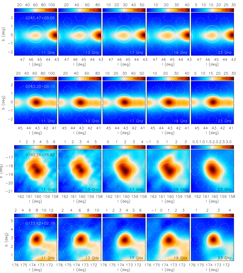
Figure 2: Subsample of $1^{\circ}$ smoothed intensity maps in Galactic coordinates. Fom left to right: QUIJOTE-MFI intensity maps at 11 GHz (horn 3), 13 GHz (horn 3), 17 GHz (horn 2 and 4), 19 GHz (horn 2 and 4), and WMAP intensity maps at 23 GHz. From top to bottom the sources shown are the well-known Galactic supernova remnant NRAO601 (G045.47+00.06), star forming region W49 (G043.20-00.10), Perseus molecular cloud (G160.26-18.62) and the cluster S235 (G173.62+02.79). In each plot the central circle shows the aperture used to obtain the density flux estimates. The eight dashed circles show the positions of the apertures used to calculate the uncertainties on these fluxes as explained in section 3.2.

3.2 Aperture photometry

In this work we conduct a component separation analysis of the various components in intensity contributing to the total emission of each source based on a SED analysis. In intensity this method consists in calculating the total emission of a given source at each frequency. Once a SED has been calculated one can use modelling to assess the fraction of the total intensity emission associated with the different components (synchrotron, free–free, thermal dust, and AME) at all frequencies. SED modelling analysis has been widely used in the literature (e.g., Watson et al., 2005; Planck Collaboration et al., 2011; López-Caraballo et al., 2011; Planck Collaboration et al., 2014a; Génova-Santos et al., 2015, 2017; Poidevin et al., 2019).

The maps of pixel size $N_{\mathrm{side}}=512$ in the HEALPix pixelization scheme (see Górski et al., 2005) are first smoothed to $1^{\circ}$. To calculate the total emission at each frequency, the maps in CMB thermodynamic units (K_CMB) are first converted to Rayleigh-Jeans (RJ) units (K_RJ) at the central frequency, then all the maps are converted to units of Jy pixel^-1 using $S=2k_{b}T_{\rm RJ}\Omega\nu^{2}/c^{2}$, where $k_{b}$ is the Boltzmann constant, $T_{\rm RJ}$, is the Rayleigh-Jeans temperature, $\Omega$ is the solid angle of the pixel, $\nu$ is the frequency and $c$ is the speed of light. The pixels are then summed in the aperture covering the region of interest to obtain an integrated flux density. An estimate of the background is subtracted using a median estimator of pixels lying in the region defined as the background region.

In Section 3.4 we provide some comparisons with the results obtained by PIRXV. To do so, we use the same apertures and annulus used in that paper, i.e. $r_{\rm APERTURE}=60^{\arcmin},r_{\rm ANNULUS(IN)}=80^{\arcmin}$ and $r_{\rm ANNULUS(OUT)}=100^{\arcmin}$. This method, also used in previous works, relies on the pixel-to-pixel scatter in the background annulus to obtain an estimate of the uncertainty in the flux density estimate. This technique is straightforward in the case of uncorrelated noise. However, in our case there is pixel-to-pixel correlated noise, due to instrumental 1/f noise and to beam-averaged sky background fluctuations, whose correlation function is not easy to be reliably characterised. We instead apply aperture photometry at the central position of each source in the standard manner, and then the calculations are repeated eight times such that we perform flux-density integrations on eight independent disks of radius $r_{\rm APERTURE}=30^{\arcmin}$ with central coordinates distributed along a circle with radius 2^∘ around the source (as shown in Figure 2). The final uncertainty is obtained from the scatter of these eight flux-density estimates. This procedure is used for all sources except for the California region for which the background structure is complex and was producing bad fits such that $\nu_{\rm AME}$= 60.0 $\pm$0.0 GHz, i.e. the prior upper limit. For that region we therefore use the same aperture and background annulus as in PIRXV and we expect our uncertainties on the fluxes of this region to be slightly underestimated.

3.3 Model fitting

For each source the flux density $S$ from the aperture photometry is fitted by a simple model consisting of the free-free, synchrotron (if appropriate), thermal dust, AME and CMB components:

$$S_{\rm total}=S_{\rm ff}+S_{\rm sync}+S_{\rm td}+S_{\rm AME}+S_{\rm CMB}.$$ (1)

The free–free spectrum shape is fixed and the free-free flux density, $S_{\rm ff}$, is calculated from the brightness temperature, $T_{\rm ff}$, using the expression:

$$S_{\rm ff}=\frac{2k_{b}T_{\rm ff}\Omega\nu^{2}}{c^{2}},$$ (2)

where $\Omega$ is the solid angle of our $60^{\arcmin}$ aperture. The brightness temperature is calculated with the expression:

$$T_{\rm ff}=T_{\rm e}(1-e^{-\tau_{\rm ff}}),$$ (3)

where, following Draine (2011) the optical depth, $\tau_{\rm ff}$, is given by

$$\tau_{\rm ff}=5.468\times 10^{-2}T_{\rm e}^{-1.5}\nu_{9}^{-2}\text{EM}g_{\rm ff},$$ (4)

where $T_{\rm e}$ is the electron temperature in Kelvin, $\nu_{9}$ is the frequency in GHz units, EM is the Emission Measure in units of pc cm^-6, and $g_{\rm ff}$ is the Gaunt factor, which is approximated as:

$$g_{\rm ff}=\rm ln(\exp[5.960-\frac{\sqrt{3}}{\pi}\rm ln({Z_{i}\nu_{9}}T_{\rm e,4}^{-3/2})]+e),$$ (5)

where the charge is assumed to be $Z_{i}=1$ (i.e., hydrogen plasma) and $T_{\rm e,4}$ is in units of $10^{4}$ K. Our best estimate for the electron temperature is the median value of the Commander template within the aperture used on each source (Planck Collaboration et al., 2016c). These values lie in the range 5 458–7 194 K. The only remaining free parameter associated with the free–free component is the free–free amplitude, which can be parameterized by the effective EM.

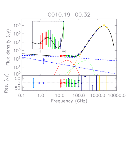
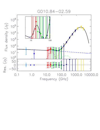
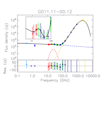
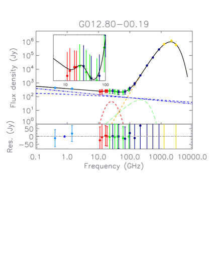
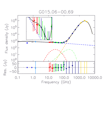
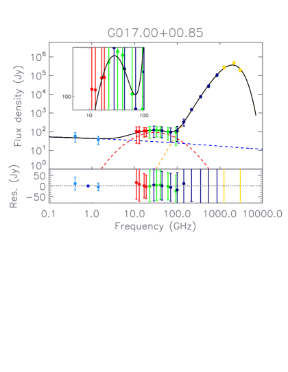
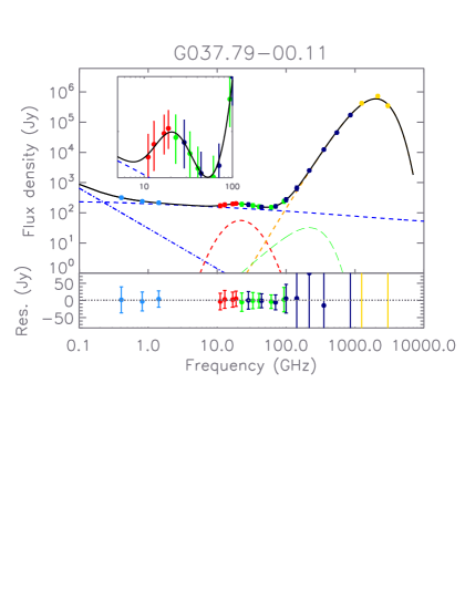
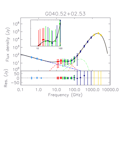
Figure 29: SED of the sample of regions discussed in this work. See caption of Figure 4 for symbols, lines and colours conventions.

Equation 4 tells that the turnover frequency that marks the transition between the optically-thick and optically-thin regimes ($\tau_{\rm ff}\approx 1$) depends on the emission measure (as EM^1/2) and on the electron temperature. In order to properly trace the degeneration between the free-free amplitude and the turnover frequency, instead of working with integrated quantities we would have to reconstruct EM along individual lines of sight inside each region and then integrate. Given the non-linear dependency of the flux density on EM, the two procedures are not equivalent, and this typically results in our fitted spectra having smaller turnover frequencies. For this reason, in cases where the data clearly shows the turnover frequency to be above 0.408 GHz (see e.g. G$015.06-00.69$ in Figure 29), in order to avoid the free-free (AME) amplitude to be biased low (high) we do not use in the fit the points with frequencies below 1.42 GHz (depicted in these cases by a blue asterisk in Figure 29).

The synchrotron component is fitted by a single power law given by:

$$S_{\rm sync}=S_{\rm synch,1GHz}\cdot\left(\frac{\nu}{\rm GHz}\right)^{\alpha_{\rm synch,int}},$$ (6)

where the two parameters that are fitted for are the spectral index, $\alpha_{\rm synch,int}$, and the amplitude at 1 GHz, $S_{\rm synch,1GHz}$. This synchrotron component is included in the fits only for a few sources (G$010.19-00.32$, G$012.80-00.19$, G$037.79-00.11$, G$040.52+02.53$, G$041.03-00.07$ and G$045.47+00.06$) as indicated in Table 7. This choice was based on the slope of the low-frequency flux densities. The first three and the last of these sources are SNRs, as listed in Table 2. There is yet another source classified as SNR in our sample, G$118.09+04.96$. However the low-frequency data do not show any hint of synchrotron emission in this source, and actually the addition of this component to the fit has no impact on the fitted AME spectrum.

The CMB is modelled using the differential of a blackbody at $T_{\rm CMB}$ = 2.7255 K (Fixsen, 2009):

$$S_{\rm CMB}=\eta\frac{2k_{b}\Omega\nu^{2}}{c^{2}}\Delta T_{\rm CMB},$$ (7)

where $\eta=x^{2}\cdot$exp$(x)/($exp$(x)-1)^{2}$ and $x=h\nu/(k_{b}T_{\rm CMB})$ is the conversion between thermodynamic and RJ brightness temperature, and $\Delta T_{\rm CMB}$ is the CMB fluctuation temperature in thermodynamic units.

Spinning dust models have many free parameters, which are extremely difficult to constrain jointly. As a result, using a phenomelogical model, which traces well the data and the typical spinning dust models, is common practice in the field. In this work the AME component is fitted by the phenomenological model consisting of an empirical log-normal approximation, first proposed by Stevenson (2014). The log-normal model is described by the following equation:

$$S_{\rm AME}=A_{\rm AME}\cdot\rm exp\left(-\frac{1}{2}\cdot\left[\frac{\rm ln(\nu/\nu_{\rm AME})}{W_{\rm AME}}\right]^{2},\right)$$ (8)

where the three free parameters are the width of the parabola $W_{\rm AME}$, the peak frequency $\nu_{\rm AME}$, and the amplitude of the parabola at the peak frequency $A_{\rm AME}$. Some previous works (e.g., Génova-Santos et al., 2017) have used a different phenomelogical model proposed by Bonaldi et al. (2007). However we note that in this model the AME peak frequency and the AME width are not independent parameters. Hence, we prefer to use the Stevenson (2014) model, which does not have this coupling.

The thermal dust emission is modelled by a single-component modified blackbody relation of the form,

$$S_{\rm td}=\tau_{250}(\nu/1200\rm GHz)^{\beta_{\rm dust}}\it B_{\nu}(T_{\rm dust}),$$ (9)

where $\tau_{250}$ is the averaged dust optical depth at 250$\,\mu$m, $\beta_{\rm dust}$ is the averaged thermal dust emissivity, and $B_{\nu}$ is the Planck’s law of the black-body radiation at the temperature, $T_{\rm dust}$, which is the averaged dust temperature.

The fit procedure includes priors on some of the parameters and consists of a minimization process using non-linear least-squares fitting in Interactive Data Language (IDL) with MPFIT (Markwardt, 2009). The errors on the fitted parameters in this method are computed from the input data covariance, and neither the goodness of the fit nor parameter degeneracies are taken into account. It must then be noted that parameter errors are sometimes underestimated. This is the case for instance when it is hard to separate the free-free and the spinning dust components. In those cases the errors on EM and $A_{\rm AME}$ will tend to be underestimated. A more reliable error estimate would require full sampling of the probability distribution and will be considered in future similar studies. Such a method should help to refine our results but would not change our main conclusions.

Flat priors are used on the following list of parameters: $T_{\rm dust}$, $\beta_{\rm dust}$, $\Delta T_{\rm CMB}$, $A_{\rm AME}$, $\nu_{\rm AME}$ and $W_{\rm AME}$. Dust temperatures, $T_{\rm dust}$, are allowed in the temperature range 10–35 K while dust index emissivities, $\beta_{\rm dust}$, are allowed in the range 1.2–2.5. Both priors are representative of average dust physical conditions in the diffuse interstellar medium (ISM) and molecular clouds. The CMB fluctuation temperatures, $\Delta T_{\rm CMB}$, are allowed to vary in the temperature range $\pm$125 K. This range of values is representative of the CMB fluctuation temperatures one can expect when operating aperture photometry including a background subtraction. The AME amplitude, $W_{\rm AME}$, is allowed to vary in the range 0–300 Jy. The AME frequency, $\nu_{\rm AME}$, is allowed to vary in the frequency range 10–60 GHz, and for the width parameter $W_{\rm AME}$, we use a prior 0.2–1.0. While spinning dust models computed for representative ISM environments (Draine & Lazarian, 1998; Ali-Haïmoud et al., 2009) typically have maximum widths corresponding to $W_{\rm AME}\approx 0.7$ we prefer not to be so strongly model constrained and allow for slightly wider AME spectra. More details on the effect of the priors used to model the AME are discussed in Section 4.3 and Table 3, in Section 5.1.5, and in Section 5.1.6.

Colour corrections for QUIJOTE, WMAP, Planck and DIRBE, which depend on the fitted spectral models, have been applied using an iterative procedure that involves calls to a specifically developed software package. This code, which will be described in more detail in Génova-Santos et al. (2023), uses as input the fitted spectral model in each iteration, which is convolved with the experiment bandpass. Colour corrections are typically $\lesssim 2\%$ for QUIJOTE, WMAP and Planck-LFI, and $\lesssim 10\%$ for Planck-HFI and DIRBE, which have considerably larger bandwidths. Colour corrections for low-frequency surveys, which have much narrower bandpasses, are not necessary.

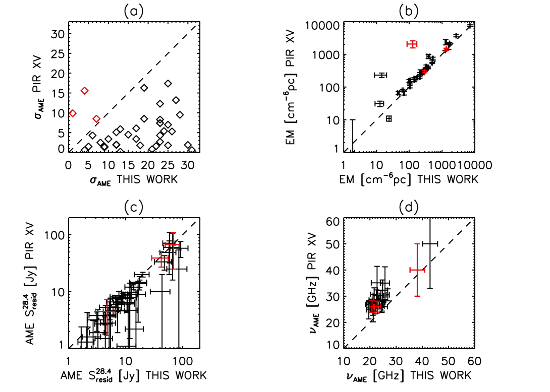
Figure 3: Comparison between the results obtained with our analysis and in PIRXV for the AME significance $\sigma_{\rm AME}$ defined as the ratio of the flux density of AME at the frequency peak position divided by the uncertainty on this estimate (a), the emission measure EM (b), the residual AME flux density at 28.4 GHz (c) and the AME peak frequency (d). Our analysis includes the QUIJOTE-MFI data. The data shown in red correspond to sources for which the significance of the AME detection is higher in PIRXV than in our analysis.

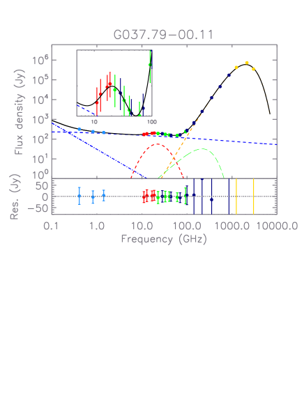
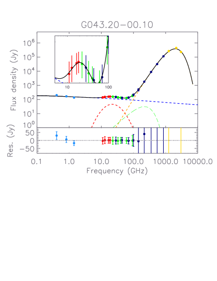
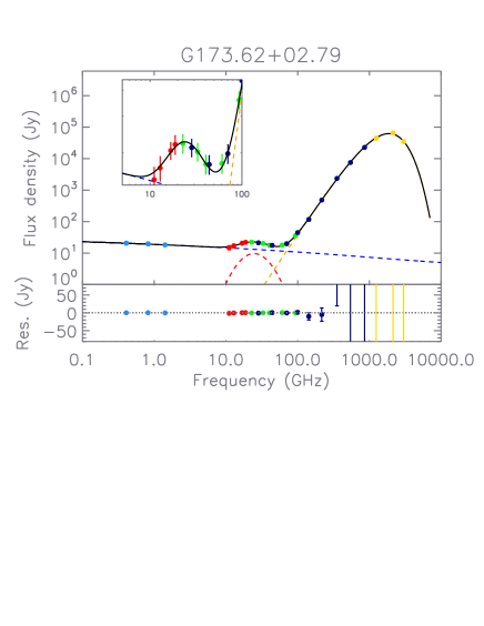
Figure 4: SED of the sample of regions shown in Figure 2. The QUIJOTE intensity flux densities are shown with red points, and the WMAP, Planck, and DIRBE intensity flux densities are shown with green, blue, and yellow< points, respectively. The low frequency points are shown in pale blue. The result of the multicomponent fit is illustrated by the continuous black curve. The fit to the AME component is shown with the dashed red line. The fit to the free–free component is shown with the dashed blue line. The fit to the thermal dust component is shown with the dashed yellow line. The fit to the CMB component is shown with the dashed green line. A zoom on the AME bump is shown in the subpanel. Residuals to the fits are shown in the bottom plots.

3.4 Comparison with AME sources previously characterized in Planck Intermediate Results XV

Before making an analysis of the full sample of 52 candidate AME sources displayed in Table 2 we first compare the results obtained with a multicomponent analysis of the SEDs calculated on the sample of 42 sources already studied by PIRXV. The AME model used by PIRXV assumes a spinning dust model corresponding to the warm ionized medium (WIM) with a peak at 28.1 GHz to give the generic shape for which only the amplitude of the peak and the peak frequency were fitted for. This horizontal shift in frequency is artificial, as the WIM model, with the parameters that have been used do produce that model, predicts a precise value for $\nu_{\rm peak}$. On the contrary, as explained before, the AME model used in our analysis is a phenomenological model with three parameters including one parameter to fit for the width of the bump of the AME.

To build the SEDs in the same way as PIRXV, as mentioned before, we use an aperture of radius $60\arcmin$ and an annulus of internal and external radii of sizes $80\arcmin$ and $100\arcmin$, respectively. For this comparison, we then use the parameters obtained by PIRXV on the CMB and thermal dust components as fixed input parameters and then we fit our model of AME, free-free and synchrotron (in the cases where the synchrotron was considered in the fits by PIRXV, i.e. on sources G$010.19-00.32$, G$012.80-00.19$, G$037.79-00.11$, G$045.47+00.06$ and G$118.09+04.96$). From these fits we calculate the AME significance ($\sigma_{\rm AME}$) as the ratio of the flux density of AME at the frequency peak position divided by the uncertainty on this estimate. The results are displayed in Figure 3 (a). Three points show a higher AME significance in PIRXV than in our analysis (data shown with red colour in the plots). Overall, however, our analysis shows that for most of the sources the AME amplitude, and its significance are higher once the QUIJOTE data are included (data shown with black colour in the plot). This trend can be explained by the level of free-free detection to be generally higher in the PIRXV analysis than in our component separation analysis as shown in Figure 3 (b). This point is also confirmed by the higher level of AME obtained with our analysis compared to the level of AME detected by PIRXV at a frequency of 28.4 GHz as displayed in Figure 3 (c). In this plot AME $S^{28.4}_{\rm resid}$ is the AME flux obtained from the modelling at 28.4 GHz. This general trend is consistent with the results obtained by Génova-Santos et al. (2017), by Poidevin et al. (2019) and by Fernandez-Torreiro et al. (2023), and confirms that the QUIJOTE-MFI data are crucial to help breaking the inevitable degeneracy between the AME and the free-free that occurs when only data above 23 GHz are used in regions with AME peak flux densities close to this frequency. From Fig. 3 (d) it is also clear that the inclusion of QUIJOTE data favours lower AME peak frequencies, which are found to be on average around 4 GHz smaller than in PIRXV. It is also worth stressing that the addition of QUIJOTE data clearly leads to a more precise characterisation of the emission models in the $10-60\,$GHz frequency range. We find on average errors smaller by $\approx 30\,\%$ on $EM$ and $A_{\rm AME}$, by $\approx 70\,\%$ on $W_{\rm AME}$, by $\approx 60\,\%$ on $\nu_{\rm AME}$ and even by $10\,\%$ on $\beta_{\rm dust}$ and $T_{\rm dust}$.

To test that our interpretation of the results is not model-dependent we repeated the analysis described above with the model proposed by Bonaldi et al. (2007). The final plots are very similar to those displayed in Figure 3 meaning that the higher level of detection of AME comes from the addition of the QUIJOTE maps at 10–20 GHz. In addition to this, our model should provide more reliable estimates of the AME peak frequency thanks to it being fully independent on the AME width.

4 Regions of AME

In the following sections we describe the level of detection of AME derived from the modelling analysis of the SEDs (Section 4.1) and their possible contamination by UCH ii regions (Section 4.2). From this analysis we define the final sample of candidate AME sources that will be used for further statistical studies. Additional calculations used to test the robustness and validate this sample are given in Section 4.3.

4.1 Significance of AME detections in our sample

In order to make a study of the detection of AME in the 52 sources from our sample we first produced a series of intensity maps at all available frequencies. The maps were inspected and removed if some pixels were showing no data in the aperture or annulus areas; this process affecting more specifically low frequency maps.

The component separation was operated by including fits for the free-free, the AME, the thermal dust and the CMB components. The synchrotron component was also included in the six sources indicated in Section 3.3. Each SED was then inspected by eye and it was found that most of the sources were showing the detection of a bump in the frequency range 10–60 GHz. Some examples of SEDs in intensity are shown in Figure 4.

The histogram displayed in Figure 5 shows the distribution of the significance of the AME detection, $\sigma_{\rm AME}$. Following PIRXV we define the sources with $\sigma_{\rm AME}>5$ as “significant AME sources”, the sources with $2<\sigma_{\rm AME}<5$ as “semi significant AME sources”, and the sources with $\sigma_{\rm AME}<2$ as “non AME detections”. Some of the “significant AME sources” are re-classified as “semi-significant AME sources” as will be discussed in the next section. The concerns regarding modelling problems and systematic errors for a few sources are discussed in Section 4.3.

Figure 5: Histogram of the AME significance values ($\sigma_{\rm AME}$) for the sample of 52 sources. The 5$\sigma$ limit is shown with the vertical dashed line. Sources that are significant and have a maximum contribution from UCH ii regions, $f^{\rm{UC}\sc{H\,II}}_{\rm max}<0.25$, are shown as the filled histogram.

4.2 Ultra-Compact Hii regions

Ultra-Compact H ii regions (UCH ii) could bias AME detections and change the free-free typical behaviour. It is therefore important to assess their possible impact on our analysis. UCH ii with EM $\gtrsim 10^{7}$ cm^-6pc are expected to produce optically thick free-free emission up to 10 GHz or higher (Kurtz, 2002, 2005). To take into account possible contamination of our sample by emission from arcsec resolution point sources (Wood & Churchwell, 1989a) that are not AME in nature we follow the method used in PIRXV as illustrated by their Figure 5. To this aim we catalog all the IRAS points sources retrieved from the IRAS Point Source Catalog (PSC) that lie inside the 2^∘ diameter circular apertures of our sample. These sources are classified as a function of their colour-colour index defined by the logarithm of flux ratios obtained in several bands. The PSC UCH ii potential candidates tend to have ratios log${}_{10}(S_{60}/S_{12})\geq 1.30$ and log${}_{10}(S_{25}/S_{12})\geq 0.57$ (Wood & Churchwell, 1989b). They are identified accordingly. Kurtz et al. (1994) measured the ratio of 100$\,\mu$m to 2 cm (15 GHz) flux densities and found it lies in the range 1000–400000, with no UCH ii regions having $S_{100\mu m}/S_{2\rm cm}<1000$. Following PIRXV we use this relation to put limits on the 15 GHz maximum flux densities that could be emitted by candidate UCH ii regions encountered in the apertures used for measuring the flux densities of our sample of sources. The fluxes at 100 $\mu$m of the PSC sources are summed up toward each aperture and then divided by 1000 to get an estimate of the the maximum UCH ii flux density at 15 GHz, $S_{\rm max}^{\rm UCHII}$, towards each candidate AME source. From the multicomponent fits, the flux densities at 15 GHz (or 2 cm) are calculated and compared to these maximum UCH ii flux densities. The distribution is shown in Figure 6 where the maximum UCH ii flux densities are plotted against the 15 GHz flux densities obtained with our analysis. If a candidate AME source detected with more than 5$\sigma$ has a residual AME flux density at 15 GHz lower than 25$\%$ of the maximum UCH ii flux density then it is re-classified as “semi-significant”, as indicated in Table 2. We believe that this is a very conservative approach, in a way that many of these re-classified sources are actually “significant” AME detections. UCH ii contributions to the 30 GHz excess have been recently investigated by Rennie et al. (2021) on a small sample of galactic H ii regions using data from the 5 GHz CORNISH catalog. The study rejects such regions as the cause of the AME excess.

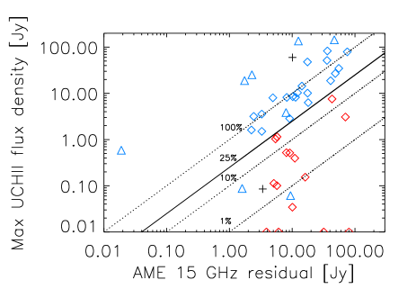
Figure 6: Estimated maximum contribution from UCH ii regions against 15 GHz AME residual flux density. The most significant AME sources ($\sigma_{\rm AME}>5$ and $S_{\rm 15}^{\rm residual}>0.25\times S_{\rm max}^{\rm UCHII}$) are shown as red diamond symbols, while non-AME regions ($\sigma_{\rm AME}<2$) are shown as dark cross symbols. “Semi-significant” AME sources ($\sigma_{\rm AME}=$2–5) are shown as blue triangle symbols. “Significant” AME regions that have a potentially large contribution from UCH ii ($S_{\rm 15}^{\rm residual}<0.25\times S_{\rm max}^{\rm UCHII}$) are re-classed as “semi-significant” and are highlighted by blue diamonds. The data shown with red diamond symbols are the “Significant” AME regions such that $S_{\rm 15}^{\rm residual}>0.25\times S_{\rm max}^{\rm UCHII}$, if this information is available. Regions with no matched UCH II regions are set to 0.01 for visualization and lie on the bottom of the plot. The dashed lines correspond to different maximum fractions of UCH ii flux density: 1, 10, 25 (solid line), and 100$\%$ of the 15 GHz residual flux density.

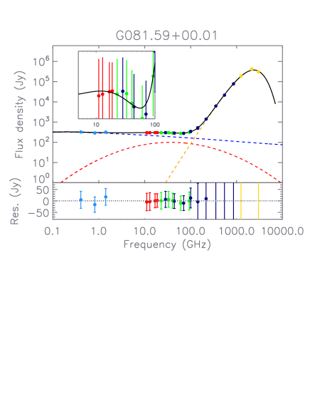
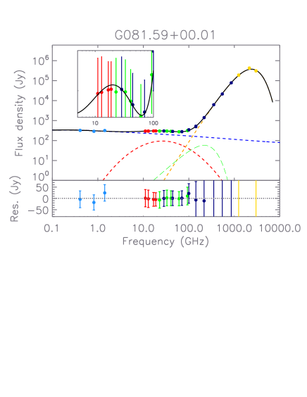
Figure 7: Two multicomponent fits of the DR23$/$DR21 region. Colours and symbols definitions are the same as in Figure 4. Left: fits obtained with priors on the AME parameters such that $10<\nu_{\rm AME}<60\,$ GHz, and $0.2<W_{\rm AME}<2.5$. Right: Same as left but with $0.2<W_{\rm AME}<1$. A discussion about the choice of priors is given in section 4.3. The AME and CMB components fit parameters obtained in each case are displayed in Table 3.

DR23/DR21	$A_{\rm AME}$	$\sigma_{\rm AME}$	$\nu_{\rm AME}$	$W_{\rm AME}$	$\Delta T_{\rm CMB}$	$A_{\rm AME}$ priors	$\nu_{\rm AME}$ priors	$W_{\rm AME}$ priors	$\chi^{2}_{\rm red}$
[G081.59+00.01]	[Jy]		[GHz]		[Jy]	[Jy]	[GHz]
See plot on Figure 7, left	99.4 $\pm$ 5.7	17.4	36.8 $\pm$40.5	1.8 $\pm$ 1.2	-1.2 $\pm$ 69.6	[0 , 300]	[10 , 60]	[0.2 , 2.5]	0.18
See plot on Figure 7, right	94.0 $\pm$ 5.2	18.1	26.3 $\pm$ 3.6	1.0	125.0	[0 , 300]	[10 , 60]	[0.2 , 1.0]	0.20

Table 3: Fit parameters of the AME and CMB components obtained with different priors on the AME width parameter, $W_{\rm AME}$. Note that in the case of stronger priors the best-fit values for $W_{\rm AME}$ and $\Delta T_{\rm CMB}$ are found in the border of the prior. The corresponding plots are shown in Figure 7.

4.3 Robustness and validation

The significance of AME detection, defined by the parameter $\sigma_{\rm AME}$, discussed in section 4.1, is an important indicator reflecting the ability of our analysis to detect and fit any excess of emission observed in the frequency range 10–60 GHz; whether such a bump is potentially dominated by UCH ii regions or not (Section 4.2). The significance of AME detection obtained on each source, though, is also dependent on the overall accuracy of the multicomponent fit obtained over the full frequency spectrum considered in the analysis.

In order to explore the stability of the fitting procedure we made a number of tests to check that our main results are not affected by our fitting method and assumptions. This includes relaxing the assumed calibration uncertainty and changing the sizes of the aperture and annulus radius. Overall we were able to fit all the 4 or 5 components on 46 sources from the 52 sources included in the initial sample, or in other words the multicomponent fit was converging on all the components considered to fit each of the 46 sources.

The SPDust2 models (see Ali-Haïmoud et al., 2009; Ali-Haimoud, 2010) for cold neutral medium, dark cloud, molecular cloud, warm ionized medium and warm neutral medium have widths lying in the range $[0.4-0.7]$ while in practice slightly wider distributions could be expected (see discussion in Section 3.3). To take this into account the uniform priors used on the AME parameters are: $10<\nu_{\rm AME}<60\,$ GHz, and $0.2<W_{\rm AME}<1.0$. Such assumptions on the values allowed to be taken by $W_{\rm AME}$ are important to keep realistic AME detections. An example of the effect of the priors is shown in Figure 7 where multicomponent fits obtained on the DR23$/$DR21 maps are displayed. The plot on the left shows the fit on the AME component with priors on $W_{\rm AME}$ such that $0.2<W_{\rm AME}<2.5$, while the plot on the right displays the AME fit component with priors on $W_{\rm AME}$ such that $0.2<W_{\rm AME}<1.0$. The AME fit parameters obtained in both cases are given in Table 3. In the case of loose priors on $W_{\rm AME}$ the AME component shows an excessively wide looking bump, even if the improvement in the goodness of the fit is marginal (see the values of the $\chi^{2}_{\rm red}$ in Table 3). Such a broad spectrum cannot be reproduced by spinning dust models for environments with reasonable physical parameters, so models like this might be deemed as physically unrealistic. This demonstrates the need for setting realistic priors on the fits to overcome the problem with fit degeneracies. Finally, as it was commented in Section 3.3, our methodology for error estimation do not properly grasp those parameter degeneracies, leading in some cases to an underestimation of the error (see the too small error of $\nu_{\rm AME}$ in the case of strong prior in Table 3).

As a final test we repeated the analyses with more stringent priors such that $0.4<W_{\rm AME}<0.7$ and 16 GHz $<\nu_{\rm AME}<$ 60 GHz, and found that this does not have a strong impact on the derived results. In particular, we found differences typically smaller than $5\,\%$ in $\nu_{\rm AME}$ and typically smaller than $20\,\%$ in $A_{\rm AME}$.

Our final sample follows the superscript symbols given in the last column in Table 2. A total of 6 sources (labelled as “BD”) considered as bad detections of AME because of a bad fit of the AME, of the free-free or of the thermal dust component, are not considered on a statistical basis. On the other hand, statistics are given for the sample which we refer to as the selected sample (46 sources). This data set includes sources with low or poor AME detection (2 sources, labelled as “LD”), with “semi-significant” AME detection (29 sources labelled as “SS”, including 20 “significant” AME sources reclassified as "semi-significant AME sources") and with “significant" AME detections (15 sources labelled as “S”). Statistics are also given on the sample of “semi-significant” AME detections and on the sample of “significant” AME detections. The selected sample includes a total of 7 sources with fits reaching the prior upper limit on $W_{\rm AME}$ and such that, the uncertainty on this parameter is, $\sigma_{W_{\rm AME}}=0$. These sources are included in the sample of AME well-detected 44 sources (i.e., the sample including “semi-significant” and “significant” AME detections).

5 Statistical study of AME sources

Along this section we study the statistical properties of the physical parameters of the sample discussed in the previous section, with the aim of better understanding the physical and environmental conditions of the AME sources, as well as to obtain insights about the nature of the carriers that cause the AME. The parameter values used to model the components estimated from the analysis of the SEDs in intensity are given in Tables 7 and 8. The method used to calculate the flux densities does not take into account the effect of the signal integration through the thickness of the clouds as well as across the area sustended by each telescope. This limitation will be taken into account, as much as possible, in the interpretation of the results.

5.1 Nature of the sources

In this section we focus our analysis on the parameters used to model the AME and some of the thermal dust component parameters. This includes the relative strength of the ISRF, which is estimated from the fitted thermal dust parameters.

5.1.1 AME fraction at 28.4 GHz

As a first step we investigate the fraction of the total flux density at 28.4 GHz that is produced by AME under the expectation that free-free and AME are the dominant sources of radiation at this frequency. For this we calculated the residual AME flux density at $28.4\,$GHz, $S^{28}_{\rm res}$, by subtracting to the measured flux density at this same frequency all the other components and propagating their uncertainties. The histogram of this quantity is plotted in Figure 8 and shows that regardless of whether the sources are classified as “significant” or “semi-significant”, the contribution of the AME flux density goes from a few per cent to almost 100 per cent of the total flux density. This result is different from that obtained by PIRXV who found that in their sample the sources classified as “significant” AME sources were mainly showing $S^{28}_{\rm res}/S^{28}>50\,\%$, while the remaining sources classified as “semi-significant” were lying in the lower part of the histogram such that $S^{28}_{\rm res}/S_{28}\lesssim 50\,\%$. All in all, the majority of the sources in our selected sample show $S^{28}_{\rm res}/S^{28}<50\,\%$. This result could come from the AME peak frequency distribution which is found to be about 4 GHz lower than by PIRXV. This result will be presented in Section 5.1.5.

Figure 8: Histogram of the AME fraction $S^{28}_{\rm res}/S_{28}$ at 28.4 GHz. The selected sample is shown as the unfilled histogram. The “significant” AME detection sample is shown with the hatched area.

5.1.2 Dust properties

The distribution of the thermal dust temperature, $T_{\rm dust}$, against the thermal dust emissivisity, $\beta_{\rm dust}$ obtained from the SEDs multicomponent fits are displayed in Figure 9. The expected anti-correlation that is discussed and analysed in many works (e.g., Paradis et al., 2014) is also seen in the plot.

An apparent sequence in the IRAS colours given by the $12\mu$m$/25\mu$m and $60\mu$m$/100\mu$m ratios can also be expected from previous studies of H ii regions (Chan & Fich, 1995; Boulanger et al., 1988), and external galaxies (Helou, 1986) showing an anti-correlation between the two ratios. The interpretation relates to the spatial distribution of different grain populations as a function of the Inter-Stellar Radiation Field (ISRF) intensity. This trend was obtained for the sample of sources discussed by PIRXV. We find a result similar to their analysis but our plots shown in Figure 10 presents a lower dynamic range of the colour ratio $60\,\mu\text{m}/100\,\mu\text{m}$ than the one from their analysis. Our sample probes line-of-sights (LOSs) with colour ratios $60\,\mu\text{m}/100\,\mu\text{m}$ lying in the range 0.2–0.7, which is the range in which PIRXV found most of their sources classified as “significant” AME detections and not expected to be dominated by UCH ii region emission.

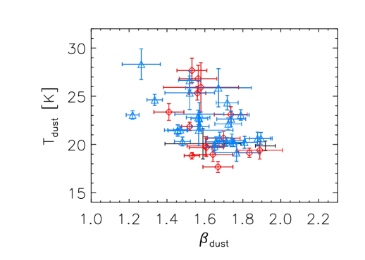
Figure 9: Distribution of the thermal dust temperature, $T_{\rm dust}$, against the thermal dust emissivisity, $\beta_{\rm dust}$ obtained from the SEDs multicomponent fits. The “significant” AME detection sample is shown with red diamonds. The “semi-significant” AME detection sample is shown with blue triangles. Low AME detections are shown in black.

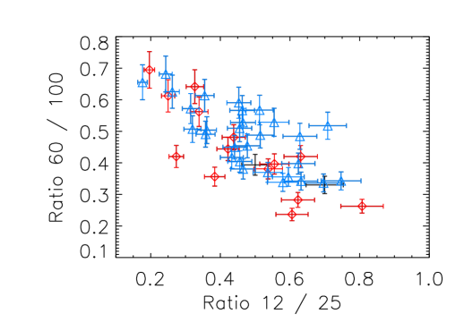
Figure 10: Colour–colour plot of IRAS $12\mu$m$/25\mu$m against $60\mu$m$/100\mu$m for the sample of sources. Symbols and colours definition are the same as in Figure 9.

5.1.3 Dust optical depth

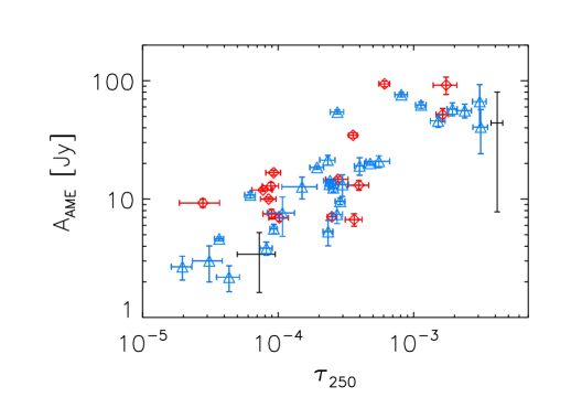
Figure 11: Distribution of the AME peak flux density A_AME against $\tau_{250}$. All selected data are displayed. Symbols and colours definition are the same as in Figure 9.

The sources of our sample are distributed across regions of different optical depths. In order to understand how this parameter could help us to build up a picture of the distribution of the parameters used to fit the AME components classified as “semi-significant” or “significant”, in Figure 11 we show the variations of the peak AME flux density, $A_{\rm AME}$, as a function of the thermal dust optical depth at 250 $\mu$m, $\tau_{250}$, obtained from the fits of the thermal dust components. One can see a clear trend showing an increase of the maximum AME flux density with the quantity of thermal dust matter encountered along the LOSs. The Spearman Rank Correlation Coefficient (SRCC) of that distribution is r${}_{\rm s}=0.80\pm 0.04$. This is not a surprise, as a strong spatial correlation was already observed between the AME and thermal dust, when AME was first detected (see Kogut, 1996; Leitch et al., 1997), and it is well established that the interstellar medium is pervaded by a complex non-uniform distribution of thermal dust material, a fraction of which spatially correlates with the spiral arms structure of the Galaxy (e.g. Marshall et al., 2006; Lallement et al., 2019) toward which many sources of our sample are located (see Figure 1). In addition, no correlation is observed between the AME peak frequencies and the thermal dust optical depths at 250$\,\mu$m, (see Figure 24). Similarily, no correlation is observed between the width of the parabola used to fit the AME and the thermal dust optical depth (see Figure 25). One can clearly see in that plot the cases for which the AME width reaches the upper limit of the prior $W_{\rm AME}=1$. These cases are not restrained to a specific range of the thermal dust optical depth parameter, which means that the AME detections with $W_{\rm AME}=1$ are not expected to depend on this parameter.

5.1.4 The interstellar radiation field: G₀

Another important parameter that is useful to describe the physics of the several environments towards AME regions is the relative strength of the ISRF, $G_{0}$ (see Mathis et al., 1983). AME carriers are believed to be tiny particles lying in the bottom part of the interstellar dust grain size spectrum ($a\lesssim 1$ nm) (possibly including Polycyclic Aromatic Hydrocarbons or PAHs). Their chemical properties, physical coherence and total charge could vary over time and from one environment to another, and therefore depend on the relative strength of the ISRF. Therefore, having our estimation of $G_{0}$ is very useful to explore possible relations with the parameters used to model the AME component detected at the SED level. An estimation of $G_{0}$ can be obtained from the equilibrium dust temperature of the big dust grains ($T_{\rm BG}$) compared to the average value of 17.5 K (see Mathis et al., 1983), with the relation:

$$G_{0}=\left(\frac{T_{\rm BG\it}}{17.5\rm{K}\it}\right)^{4+\beta_{\rm BG}},$$ (10)

where $\beta_{\rm BG}$ is the spectral index associated with the opacity of the big grains. In the following, we assume $T_{\rm BG}\approx T_{\rm dust}$, where $T_{\rm dust}$ is the averaged temperature of the thermal dust component obtained from the fit on each region. As in PIRXV, we also assume a constant value $\beta_{\rm BG}=2$. We note that using $\beta_{\rm BG}\approx\beta_{\rm dust}$ could also be considered, but would not change the conclusions of our analysis.

The correlation between the AME fraction at 28.4 GHz (defined as the residual AME flux density at 28.4 GHz divided by the total flux density at 28.4 GHz) and G₀ is shown in Figure 12. The data show a decrease of the AME fraction as a function of G₀. This trend is similar to the one obtained by PIRXV in their analysis and seems to be dependent of the considered subsets. In our analysis the slope of the “significant” AME detection data sample is of order $\gamma=-0.48$, while the slope of “semi-significant” AME detection data sample is of order $\gamma=-0.61$. We point out that the uncertainties of the values of the slopes we estimated are large, $\approx 0.8$ for both “significant” and “semi-significant” AME detections data points, which prevents a full and fair comparison with results from previous studies. Our slopes, though, can be compared to the slope of $\gamma=-0.11\pm 0.04$ obtained by PIRXV on their strongest AME sources sample (see their Figure 15 and section 5.1.4), and to the slope of $\gamma=-0.59\pm 0.11$ obtained on their semi-significant AME sources. All in all, our results agree with those of PIRXV within the uncertainties. Differences in the slopes estimates can be explained by the different sample sizes (half-sky versus full sky coverage) and by the introduction of the QUIJOTE data in our analysis.

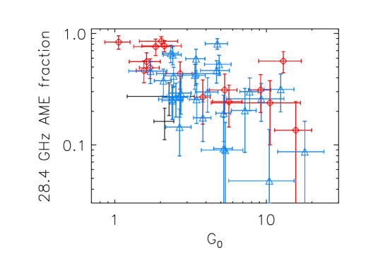
Figure 12: AME fraction at 28.4 GHz as a function of the estimated $G_{0}$. Symbols and colours definition are the same as in Figure 9.

5.1.5 Peak frequency of AME

Among the three parameters used to fit the AME components in our sample, one is the peak frequency, which is allowed to vary in the frequency range 10–60 GHz. Such a degree of freedom is important since it allows to get better final fits. It has also been shown in previous works that one can expect the frequency of AME to vary from one source to the other, or even within the same region (Cepeda-Arroita et al., 2021). The histogram of the AME peak frequency calculated for the selected sample is shown in Figure 13. The Gaussian fit to the distribution provides a mean frequency and dispersion given by 23.6 $\pm$ 3.6 GHz. The hashed histogram shows the distribution of the “significant” AME sources sample peaking around the weighted mean frequency. PIRXV found their sample of AME sources to peak in the range 20–35 GHz, with a weighted mean of 27.9 GHz, a bit higher than our mean value, the main reason of this difference being that flux densities in the frequency range 10–20 GHz were not available in their analysis. In fact, the addition of QUIJOTE-MFI data clearly helps reducing the uncertainty in the determination of $\nu_{\rm AME}$, thanks to allowing to trace the down-turn of the AME spectrum at low frequencies. Our average error on $\nu_{\rm AME}$ is 3.4 GHz, and when we repeat our analysis excluding QUIJOTE-MFI data we get an average error of 7.5 GHz (see also discussion in Section 6.3). On the other hand our analysis of G160.60-12.05 (the California nebula/NGC 1499) recovers an AME peak frequency at 49.1 $\pm$38.5 GHz, which is consistent with values obtained in previous analyses (Planck Collaboration et al., 2011, 2014a). The uncertainty on our estimate is quite large because the free-free dominates at $\nu<$100 GHz making the width of the AME bump poorly constrained and the fitted parameters strongly degenerated. On top of that the circular aperture that we use may not be optimal in this case where the emission is elongated and pretty extended.

Figure 13: Histogram of the AME peak frequency in bins of size 2 GHz. The selected sample is shown as the unfilled histogram. The “significant” AME detection sample is shown with the hashed area. A Gaussian fit to the histogram is shown with the dashed-line.

5.1.6 Width of the AME bump

In addition to the maximum flux density and peak frequency parameters, the third parameter used to fit the AME components is the width of the parabola, $W_{\rm AME}$ (see Equation 8). The allowed range in the fit was 0.2–1 and the initial value was $W_{\rm AME}=0.5$ for all sources, this value being the expected average value from the SPDust2 models. The histogram of our fitted values is displayed in Figure 14. As discussed previously, the multicomponent fits leading to output fit parameters of values $W_{\rm AME}=1$ and $\sigma_{W_{\rm AME}}=0$ are cases reaching the prior upper limit value, and this artificially leads to a higher number of sources lying in the last bin of the histogram. The selected sample is shown as the whole histogram. The single-dashed histogram shows the same distribution without the prior dominated AME detections. This distribution has a mean and dispersion given by, $W_{\rm AME}=0.58\pm 0.61$. The distribution looks rather flat, and far from Gaussian, which is reflected in the large error bar of the Gaussian fit. This in fact illustrates that $W_{\rm AME}$ is maybe the worst constrained parameter in our fit, due to large degeneracies with other parameters.

This result is obtained with a bin of size 0.1 and would need a higher sample for one to drive strong conclusions on a statistical basis. Indeed using a bin size of 0.2 the whole histogram looks rather like a normal distribution without any clear peak. Statistically, we find that $W_{\rm AME}$ does not correlate with the free-free component EM parameter. Neither do we find any correlation between $W_{\rm AME}$ and any of the thermal dust parameters. On the other hand we observe a mild correlation of $W_{\rm AME}$ with the AME emissivity ($A_{\rm AME}/\tau_{250}$). A detailed definition of the AME emissivity will be given in Section 6.2 where these results will be discussed.

Figure 14: Histogram of the width of the AME component parameterized by $W_{\rm AME}$ (see Equation 8) in bins of size 0.1. The selected sample is shown as the whole histogram. The “constrained” AME detections are shown with the unfilled histogram. The “significant” AME detection sample is shown with the double harshed area. The gaussian fit to the histogram is shown with the dashed-line.

5.1.7 Width of AME bump and peak frequency of AME

The three parameters describing the parabola used to fit the AME flux density bump (see Equation 8) are independent from each other. With this model any correlation found between the AME peak frequency and the parabola width parameter could therefore be indicative of the physics underlying the description of the AME carriers. We checked that neither a negative nor a positive correlation can be seen between the two parameters. As shown in Table 9, all the samples (selected, “semi-significant” and “significant”) are showing SRCCs consistent with a null correlation. These results show that the width and the peak frequency of the AME component are fully independent from each other, although this conclusion could be affected by the fact that, in some cases, $W_{\rm AME}$ seems to be poorly constrained in our analysis.

5.2 Dust correlations

In this section we focus on the thermal dust component with the aim to better understand its relation with the AME component. We also consider high frequency maps at 100$\,\mu$m, 60$\,\mu$m and 12$\,\mu$m, since these data have the potential to provide information about some of the candidate AME carriers (i.e., spinning dust, PAHs or fullerenes).

5.2.1 Dust flux densities at 100$\,\mu$m, 60$\,\mu$m, 25$\,\mu$m and 12$\,\mu$m

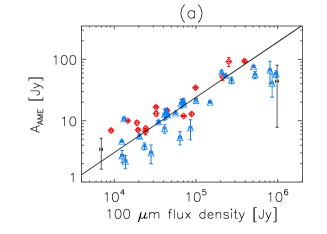
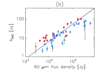
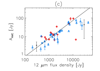
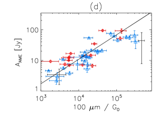
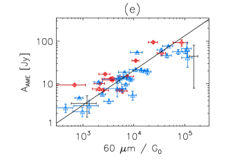
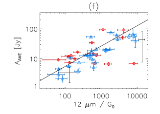
Figure 15: Top row: AME peak flux density as a function of the 100$\,\mu$m (panel a), 60$\,\mu$m (panel b) and 12$\,\mu$m (panel c) flux density. Bottom row: same as top row but after the infrared tracers of dust have been divided by $G_{0}$ (panel d, e and f, respectively). Symbols and colours definition are the same as in Figure 9. Power-law fits to the full set are shown with back solid lines. SRCCs are given in Table 4.

Wavelentgh	SRCC	SRCC	SRCC
	selected sample	AME significant	AME semi-significant
100$\,\mu$m	0.87$\pm$ 0.04 ( 0.84$\pm$ 0.05 )	0.86$\pm$ 0.02 ( 0.65$\pm$ 0.08 )	0.89$\pm$ 0.03 ( 0.88$\pm$ 0.05)
60$\,\mu$m	0.84$\pm$ 0.04 ( 0.86$\pm$ 0.05 )	0.82$\pm$ 0.03 ( 0.65$\pm$ 0.08 )	0.88$\pm$ 0.03 ( 0.90$\pm$ 0.05)
25$\,\mu$m	0.85$\pm$ 0.04 ( 0.81$\pm$ 0.05 )	0.65$\pm$ 0.03 ( 0.43$\pm$ 0.07 )	0.90$\pm$ 0.03 ( 0.90$\pm$ 0.05)
12$\,\mu$m	0.80$\pm$ 0.04 ( 0.70$\pm$ 0.05 )	0.39$\pm$ 0.04 ( 0.19$\pm$ 0.07 )	0.89$\pm$ 0.03 ( 0.85$\pm$ 0.06)

Table 4: Spearman rank correlation coefficients (SRCCs) between the AME maximum flux densities and the IR/submm flux densities. The values displayed between parentheses are the SRCCs obtained once the IR/submm flux densities are divided by the IRSFs estimates G₀.

Following the spatial correlation observed between AME and the thermal dust emission when AME was first discovered, many studies have explored and discussed the possibility that AME carriers are spinning dust grains in nature (e.g., Draine & Lazarian, 1998, 1999; Ali-Haïmoud et al., 2009), i.e., possibly a specific subclass of the dust grain population spectrum. A look to various dust grain emission templates should therefore be useful to explore if any specific correlation exists between the maximum AME flux densities and the flux densities of thermal dust observed at 100$\,\mu$m, 60$\,\mu$m, 25$\,\mu$m and 12$\,\mu$m. Such plots are shown in Figure 15 (top row) and the strength of the correlations described by their SRCCs are given in Table 4. We find very strong correlations between the AME flux densities and the thermal dust flux densities at 100$\,\mu$m, 60$\,\mu$m, 25$\,\mu$m and 12$\,\mu$m. This result is consistent with the one obtained by PIRXV from their analysis.

If the AME carriers are spinning dust grains, the AME component is expected to be quite insensitive to the ISRF relative strength, $G_{0}$ (Ali-Haïmoud et al., 2009; Ysard & Verstraete, 2010) while on the contrary the thermal dust grains population is expected to be sensitive to it, mainly because the UV radiation should control their temperature. If that was true one would expect better correlations between the maximum AME flux densities and the flux densities of thermal dust observed at 100$\,\mu$m, 60$\,\mu$m, 25$\,\mu$m and 12$\,\mu$m, once they are normalized by $G_{0}$. This has been discussed in some previous analysis (e.g., Ysard & Verstraete, 2010). The plots obtained once the thermal dust fluxes are normalized by $G_{0}$ are shown in Figure 15 (bottom row) and the strength of the correlations described by their SRCCs are given between parenthesis in Table 4. Contrary to what was found on their sample by PIRXV, normalizing the thermal dust templates by $G_{0}$ leads to less tight correlations. These results suggest that the AME carriers could be coupled to the thermal dust grain components rather than to a dust grain population relatively insensitive to $G_{0}$. On the other hand the dust grain size distribution is very sensitive to the ISRF, as well as to other parameters such as the dipole moments of PAHs (Ali-Haïmoud et al., 2009), meaning that the interpretation of the results obtained with plots such as those given in Figure 15 may be complicated. The role of $G_{0}$ will be discussed further in Section 5.4.

5.2.2 Thermal Dust peak flux densities

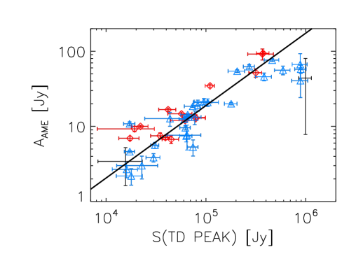
Figure 16: Maximum AME flux density versus maximum thermal dust flux density. Symbols and colours definition are the same as in Figure 9. The solid line represents a fitted power-law model to the data.

The size of the aperture used to build the SEDs could introduce a coupling between some of the thermal dust parameters $\tau_{250}$, $T_{\rm dust}$ and $\beta_{\rm dust}$ due to a possible range of degeneracy at the fit level between these parameters. In order to circumvent this problem, that could mislead the interpretation of some of the correlations discussed above, we looked at the distribution between the flux densities at the peak of the AME bumps and at the maximum of the thermal dust components. This is shown in Figure 16 where it can be seen a correlation between the two flux components at their maximum. The slope of a power-law fit to the selected sample is 0.96 and almost consistent with 1 as shown with the dark solid line on the plot. The SRRC between the two parameters is equal to 0.89 $\pm$ 0.05.

5.2.3 Thermal Dust radiance

The radiance of a component is defined as the integral of the flux density of that component over the full spectral range, $\Re=\int_{-\infty}^{+\infty}S(\nu)d\nu$. In this work, all radiances were calculated by integrating the fitted models between 0.4 and 3000 GHz, which is the frequency range where all the maps used in this analysis are available (see Table 1). Some studies have shown strong correlations between the dust radiance and the AME amplitude at the peak frequency (Hensley et al., 2016; Hensley & Draine, 2017). The distribution of both components for our sample is shown in Figure 17, (top). A good correlation is observed between the two variables of the selected sample, with a SRCC of 0.89 $\pm$ 0.05, and a power-law slope consistent with 1. This tight correlation suggests a strong coupling between the big dust grains expected to be the main contributors to the dust grain radiance considered here (i.e., in the wavelength range $\lambda>100\mu$m). Figure 17 (bottom) shows the distribution of the AME radiance $\Re_{\rm AME}$ as a function of the dust radiance $\Re_{\rm td}$. In that case a lower correlation is observed between the two parameters with a SRCC of 0.70 $\pm$ 0.06.

We believe that the reason why the AME amplitude correlates better than the AME radiance is because the latter is quite sensitive to $W_{\rm AME}$, and this parameter has large error bars due to not being very well constrained by our fit (see section 5.1.6). This said, these two correlations can be interpreted using two different views. A first one is that the AME model used to fit the data and designed to approximate the spectrum of the spinning dust emission is not fully appropriate to capture the contribution of the AME carriers, or that in some regions it is difficult to properly disentangle the AME contribution from the free-free and thermal dust contributions. Another view could be that if the AME model used to fit the data is good enough to capture the AME components accurately, then the dust radiance of PAHs and/or Very Small Grains (VSGs) could represent a relatively large contribution of the total dust radiance at wavelengths greater than 100$\,\mu$m.

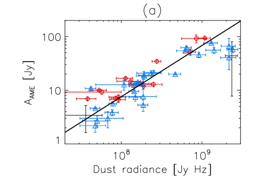
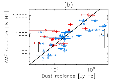
Figure 17: Top: AME flux density at peak frequency, $A_{\rm AME}$, as a function of the thermal dust radiance, $\Re_{\rm td}$. Bottom: AME radiance, $\Re_{\rm AME}$, as a function of thermal dust radiance, $\Re_{\rm td}$. Symbols and colours definition are the same as in Figure 9. The solid lines represent fitted power-law models to the data.

5.3 AME emissivity

As discussed above, strong spatial correlations were found between the AME emission and thermal dust emission when AME was first detected (see Kogut, 1996; Leitch et al., 1997). In order to build a picture of the distribution of the AME emission along the third spatial dimension (i.e., the line-of-sight, LOS), further works have defined the AME emissivity as the ratio between the AME intensity and the column density, for which the optical depth at a given wavelength is often used as a proxy (see Dickinson et al., 2018, and discussion and references therein). In order to make comparisons with results discussed in the literature we first show in Figure 18 the distribution of the AME flux density obtained by subtracting to the measured flux density at this same frequency all the other components (defined as the residual flux density at 28.4 GHz) normalized by the 100$\,\mu$m flux density ($S_{28.4{\rm GHz}}^{\rm res}/S_{100\mu{\rm m}}$), as a function of the AME detection significance. In this case the 100$\,\mu$m flux density is expected to be optically thin for a given dust temperature and composition and is used as a proxy to probe the column density of dust along the LOSs. $S_{28.4{\rm GHz}}^{\rm res}/S_{100\mu{\rm m}}$ is in the range $(0.05-9)\times 10^{-4}$ with a weighted mean of $(4.2\pm 0.3)\times 10^{-4}$ and an unweighted average of $(3.5\pm 1.6)\times 10^{-4}$ (significant AME sample). These values are consistent with each other. They are smaller than the unweighted average value of $(5.8\pm 0.7)\times 10^{-4}$ of PIRXV and than the $6.2\times 10^{-4}$ value of Davies et al. (2006) but are higher than the weighted average of $(2.5\pm 0.2)\times 10^{-4}$obtained in PIRXV and than the value of about $1.1\times 10^{-4}$ obtained by Todorović et al. (2010) on a sample of H ii regions. The differences between our estimates and those obtained by PIRXV could partially come from the different samples used in each study. Our sample only covers the North hemisphere sky while the analysis of PIRXV includes also sources in the Southern hemisphere. Different error treatment may also affect the weighted averages. Regardless of these issues, we have applied a one-to-one comparison between our flux density ratios and those reported in PIRXV in the subsample of 42 common sources. When we represent the former against the latter and fit the data to a straight line we find a slope of $0.76$, meaning that we find $\approx 30\%$ higher emissivities. This is a consequence of the increase of the AME amplitude as a result of the inclusion of QUIJOTE data (see Figure 3c and related discussion in section 6.3). A summary of these results is given in Table 5.

Sample	$S_{28.4{\rm GHz}}^{\rm res}/S_{100\mu{\rm m}}$ [$\times 10^{-4}$]
	unweighted mean	weighted mean
This work - selected sample	2.5 $\pm$ 1.7	3.7 $\pm$ 0.1
This work - semi-significant	2.1 $\pm$ 1.5	3.2 $\pm$ 0.1
This work - significant	3.5 $\pm$ 1.6	4.2 $\pm$ 0.3
PIRXV - significant	5.8 $\pm$ 0.7	2.5 $\pm$ 0.2
Todorović et al. (2010)	1.1 $\pm$ -	… $\pm$ …
Davies et al. (2006)	6.2 $\pm$ -	… $\pm$ …

Table 5: Comparison of the AME flux densities normalized by the 100$\,\mu$m flux densities obtained in this work and in previous studies.

The small range of values of the ratio of the AME residual flux density at 28.4 GHz to the flux density at 100$\,\mu$m suggests that a power-law index of order 1 could be expected between the two flux density distributions. This is indeed what the best-fitting power-law confirms as it yields a power-law index of $1.04\pm 0.21$ in tension with the power-law index of $0.67\pm 0.03$ obtained by PIRXV on their sample. Similarily, the best-fitting power-law index between the AME residual flux density at 28.4 GHz and the dust optical depth at a wavelength of 250 $\mu$m, $\tau_{250}$, yields a power-law index of $1.13\pm 0.22$ in agreement with the power-law index of $1.03\pm 0.03$ obtained by PIRXV. The results obtained by PIRXV were inferring an AME mainly proportional to the column density estimate, i.e., to the amount of material along the LOS. This is what we find whether we consider the 100 $\mu$m map or the $\tau_{250}$ parameters as proxies of the column density.

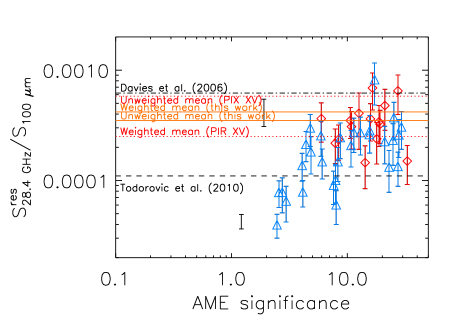
Figure 18: AME emissivity against AME significance. Symbols and their colours definition are the same as in Figure 9.

5.4 Role of the ISRF

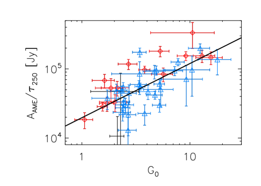
Figure 19: Variations of the AME emissivity with the relative strength of the ISRF, $G_{0}$. Symbols and colours definition are the same as in Figure 9. The power-law fit obtained on the selected sample is plotted with the black line.

The ISRF is strongly coupled to the nature of the various phases encountered in the ISM defined in terms of gas temperature and matter density. The UV light produced by the population of stars pervading the ISM is absorbed by the dust grain populations and re-radiated in the IR. The ISRF therefore plays an important dynamic role since it will affect the chemical composition of the ISM material, the dust grain distribution as well as the lifetime of the small dust grain and complex molecule populations (see Jones et al., 2013). It is therefore interesting to investigate the existence of possible relationships between the relative strength of the ISRF, $G_{0}$, and the parameters describing the AME component derived from the SEDs analysis. For this we looked at the distribution of the AME emissivity, now defined as $A_{\rm AME}/\tau_{250}$, the AME peak frequency, $\nu_{\rm AME}$, and the AME bump width parameter, $W_{\rm AME}$, as a function of $G_{0}$. The plots are shown in Figures 19, Figure 27 and Figure 28, respectively. We find poor correlations between $G_{0}$ and the AME parameters $\nu_{\rm AME}$ and $W_{\rm AME}$. On the other hand, we find a SRCC of r${}_{\rm s}=0.68\pm 0.08$ between the AME emissivity and $G_{0}$ parameters for the selected sample (Figure 19). This distribution can be fitted by a power-law of index of about 0.8 as shown with the black line in Figure 19. Since we derived the relative strength of the ISRF, $G_{0}$, by using the thermal dust grain temperature, $T_{\rm dust}$, obtained from the SED grey body fits, and by assuming a maximum and constant thermal dust emissivity, $\beta_{\rm dust}=2$ (see equation 10), the SRCCs obtained between the $A_{\rm AME}/\tau_{250}$ and $G_{0}$ parameter distributions and between the $A_{\rm AME}/\tau_{250}$ and $T_{\rm dust}$ parameter distributions are by construction identical. Similarly, the introduction of the SEDs fit estimates of $\beta_{\rm dust}$ in the calculation of $G_{0}$ only changes SRCCs values by less than one percent. This means that the AME flux densities obtained at the peak frequency are mainly correlated with the combination of the dust optical depth, $\tau_{250}$, and the thermal dust temperature $T_{\rm dust}$ parameters. This result is in agreement with the strong correlation obtained between the AME peak flux densities and $\tau_{250}$, and with the 100$\mu$m thermal dust fluxes discussed in the previous section.

In the above we have considered that a good proxy of the relative strength of the ISRF is given by $G_{0}$, which is a function of the thermal dust temperature, $T_{\rm dust}$. The EM is another interesting parameter associated with hot phases of the ISM, i.e., ionized regions. In our sample one can expect electron temperatures lying in the range 5 458–7 194 K as from the electron temperature map provided by Planck Collaboration et al. (2016c). Inside molecular clouds, the ionized regions produced by stellar radiation are expected to represent a fraction of the whole volume associated with the clouds. Not all the sources displayed in Table 2 are only molecular cloud regions in nature but they all have thermal dust along their LOSs, which is a component strongly correlated with the AME component. In this context we show in Figure 20 the distribution of the free-free EM parameter as a function of $G_{0}$. The plot shows only a poor correlation between the two parameters, this being also illustrated by the low correlation coefficient, SRCC$=0.30\pm 0.06$, found between the two parameters. This lack of correlation would indicate that the AME emissivity does not correlate significantly with the EM free-free emission parameter at Galactic scales.

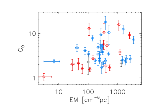
Figure 20: Free-free Emission Measure (EM) parameter as a function of the relative strength of the ISRF, $G_{0}$. Symbols and colours definition are the same as in Figure 9.

5.5 Free-Free correlations

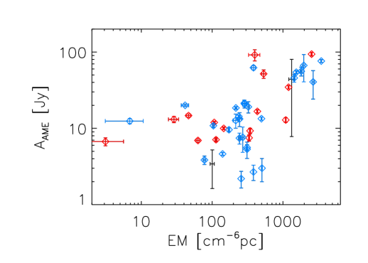
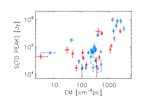
Figure 21: Top: AME flux at the peak frequency versus free-free emission measure. Bottom: Thermal dust flux at the peak frequency versus free-free emission measure. Symbols and colours definition are the same as in Figure 9.

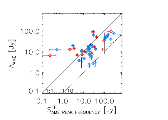
Figure 22: AME flux at the peak frequency versus free-free flux at the AME peak frequency. Symbols and colours definition are the same as in Figure 9. The one-to-one relation is displayed by the solid line and the one-to-ten relation is shown with the dashed line.

In our study the EM of the free-free does not correlate with the AME emissivity estimated by $A_{\rm AME}/\tau_{250}$. On the other hand, a mild correlation is observed between the amplitude of the AME at the peak frequency, $A_{\rm AME}$, and the EM. This is shown on the plot displayed at the top panel in Figure 21, with a SRCC between the two parameters of 0.66 $\pm$ 0.0.5. Since a strong correlation is observed between $A_{\rm AME}$ and the emission of the thermal dust at the peak frequency, $S_{\rm TD,PEAK}$, this also means that a correlation can be expected between EM and, $S_{\rm TD,PEAK}$. This is shown in the plot displayed in the bottom panel of Figure 21. In that case the SRCC between the two parameters of the selected dataset is 0.64 $\pm$ 0.04.

In the interpretation of these results it must be taken into account that our EMs are estimated directly from integrated flux densities, and given the non-linear dependency between the two, those estimates could not be representative of the real averaged EMs of each region, as it was already commented in section 3.3. This could indeed contribute to smear out any underlying real correlation. In addition, the fact that the correlation in the top panel of Figure 21 is only seen for the sources with highest AME amplitudes could be a hint that there could be a selection effect, in such a way that when the free-free is high the AME can only be detected when it is also very high. In order to better understand this, in Figure 22 we plot $A_{\rm AME}$ as a function of the flux density of the free-free at $\nu_{\rm AME}$. The one-to-one relation is displayed by the solid line while the one-to-ten relation is shown with the dashed line. Given that calibration uncertainties are of order $5-10\%$ the lack of sources below the one-to-ten line could in fact tell that the AME cannot be separated when it is less than $10\%$ of the free-free. On the contrary, the plot also shows that there are a few regions (like the Perseus and $\rho$ oph molecular clouds, respectively G160.26-18.62 and G353.05+16.90) with more AME than free-free.

It must also be taken into account that our SED multicomponent fit is subject to an anti-correlation between the AME and free-free amplitudes which may contribute to worsening the correlation observed in Figure 22. This parameter degeneracy, which upcoming 5 GHz data from the C-BASS experiment (Jones et al., 2018) will help to break, is clearly seen in MCMC analyses like those presented in Cepeda-Arroita et al. (2021) and in Fernandez-Torreiro et al. (2023).

6 Discussion

In this section we summarize our results suggesting that the AME carriers may be preferentially located in cold rather than in hot phases of the ISM. Some limitations of our modelling of the AME component are then discussed, followed by a comparisons of our results with those from previous works.

6.1 Does AME originate from the Cold ISM Phase ?

In the last sections we searched for correlations between some of the parameters obtained from the multicomponent fits of the AME component and ISM tracers including the flux densities obtained at 12, 25, 60 and 100$\,\mu$m. Interestingly, we find that the flux densities obtained at the peak frequency of the AME bumps show strong correlation with the flux densities at 100, 60 and 25 $\,\mu$m, with a small loss of correlation with the flux densities at 12 $\,\mu$m. On the other hand, once these four flux densities tracers are normalized by the relative strength of the ISRF, $G_{0}$, the correlations with $A_{\rm AME}$ are found to be about a few to ten percent lower in the high frequency bands. These results could discard tiny dust particles (PAHs or VSGs in nature) as AME carriers, if such particles are poorly sensitive to the relative strength of the ISRF. For this reason we explored in more detail possible relationships between the AME component parameters with dust modelling parameters, with $G_{0}$, as well as with the free-free component parameters. Table 6 gives a summary of some of the most relevant SRCCs obtained from the previous analysis in this respect. They could help to shed light on some existing physical relationships between the astrophysical components.

From spectral energy distribution analysis of the sample of 46 good candidate AME sources the strongest correlation is found between the maximum flux density of the thermal dust, $S_{\rm TD,peak}$, and of the AME peak, $A_{\rm AME}$ (Figure 16). A lower correlation is found between the AME emissivity, $A_{\rm AME}/\tau_{250}$, and the interstellar radiation field relative strength, $G_{0}$ (Figure 19), and a mild correlation is obtained between $A_{\rm AME}$ and the free-free EM (Figure 21, top). On the other hand no correlation is found between $A_{\rm AME}/\tau_{250}$ and $EM$ (see end of Section 5.4), and neither between the AME peak frequency, $\nu_{\rm AME}$, and $G_{0}$ (Figure 27). As discussed in the previous section, averaging effects in our estimates of EM, as well as a selection effect associated with only the brightest AME sources being detected above very high free-free amplitudes, could have an impact on the tentative correlation seen between EM and $A_{\rm AME}$. On the other hand the correlation found between $A_{\rm AME}$ and $S_{\rm TD,peak}$ is expected to be real since these two components are associated with distinct wavelength ranges with poor overlap between each other. Since there is a null correlation between $A_{\rm AME}/\tau_{250}$ and $EM$, this means that $A_{\rm AME}/\tau_{250}$, which also correlates with the dust grain emissivity, $S_{\rm TD,peak}/\tau_{250}$, is rather driven by $G_{0}$, which in turn is a function of the thermal dust temperature approximated by $T_{\rm dust}$ obtained from the modelling. In other words the interstellar radiation field still could be the main driver of the AME in terms of spinning dust excitation mechanisms, but the spinning dust could be more likely associated with cold phases of the ISM rather than to hot phases associated with free-free radiation.

Variable 1	Variable 2	SRCC	SRCC	SRCC	Power-Law Slope(a)	Figure
		selected sample	AME significant	AME semi-significant	selected sample
$A_{\rm AME}[\rm Jy]$	$S_{\rm TD,peak}[\rm Jy]$	0.88$\pm$ 0.05	0.82$\pm$ 0.07	0.91$\pm$ 0.04	0.96$\pm$1.56	16
$A_{\rm AME}[\rm Jy]$	$\Re_{\rm Dust}$	0.88$\pm$ 0.05	0.85$\pm$ 0.08	0.90$\pm$ 0.05	0.95$\pm$2.37	17 (top)
$W_{\rm AME}$	$A_{\rm AME}/\tau_{250}[\rm Jy]$	0.66$\pm$ 0.12	0.64$\pm$ 0.18	0.57$\pm$ 0.15	…	23
$A_{\rm AME}/\tau_{250}[\rm Jy]$	$G_{0}$ or Ttd	0.68$\pm$ 0.08	0.87$\pm$ 0.07	0.62$\pm$ 0.11	0.78$\pm$0.94	19
$S_{\rm TD,peak}[\rm Jy]$	EM [cm-6 pc]	0.64$\pm$0.03	0.50$\pm$ 0.08	0.64$\pm$ 0.04	0.43$\pm$0.16	21 (bottom)
$A_{\rm AME}[\rm Jy]$	EM [cm-6 pc]	0.59$\pm$ 0.05	0.65$\pm$ 0.11	0.55$\pm$ 0.03	1.42$\pm$0.89	21 (top)
$\Re_{\rm AME}$	$\Re_{\rm td}x10^{-4}$	0.70$\pm$ 0.14	0.66$\pm$ 0.23	0.73$\pm$ 0.17	1.57$\pm$4.32	17 (bottom)
$\nu_{\rm AME}[\rm GHz]$	$G_{0}$ or Ttd	0.40$\pm$ 0.12	0.21$\pm$ 0.22	0.60$\pm$ 0.15	-0.05$\pm$0.56	27
$G_{0}$ or Ttd	EM [cm-6 pc]	0.30$\pm$ 0.06	0.49$\pm$ 0.13	0.09$\pm$ 0.07	…	20
$W_{\rm AME}$	$G_{0}$ or Ttd	0.23$\pm$ 0.12	0.57$\pm$ 0.18	0.07$\pm$ 0.15	…	28
$\nu_{\rm AME}[\rm GHz]$	EM [cm-6 pc]	0.06$\pm$ 0.11	0.27$\pm$ 0.20	-0.24$\pm$ 0.14	…	…
$A_{\rm AME}/\tau_{250}[\rm Jy]$	EM [cm-6 pc]	0.01$\pm$ 0.07	0.46$\pm$ 0.14	-0.21$\pm$ 0.07	…	…
$A_{\rm AME}[\rm Jy]$	$G_{0}$ or Ttd	-0.16$\pm$ 0.06	0.26$\pm$ 0.10	-0.33$\pm$ 0.07	…	…

Table 6: Selection of Spearman rank correlation coefficients (SRCCs) between several model parameters in decreasing strength for the selected sample. ^(a): Slopes obtained from linear fits in log–log space.

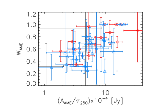
Figure 23: AME emissivity against the width of the AME parabola model, $W_{\rm AME}$. Symbols and colours definition are the same as in Figure 26.

6.2 AME components characterization

From the results obtained with the multicomponent fit analysis we tested the level of independency between the parameters used to fit the AME. This model is the analytical approximation of the spectrum of spinning dust emission proposed by Stevenson (2014). Indeed, we find null or very low correlations between parameters, $A_{\rm AME}$ and $\nu_{\rm AME}$, $\nu_{\rm AME}$ and $W_{\rm AME}$, and $W_{\rm AME}$ and $A_{\rm AME}$. On the other hand, we find a small correlation between $W_{\rm AME}$ and $A_{\rm AME}/\tau_{250}$. The distribution of these two parameters is shown in Figure 23. By definition, the AME emissivity depends on the total amount of material along the LOS as estimated by $\tau_{250}$, and this correlation means that, on average, $A_{\rm AME}/W_{\rm AME}$ is not directly proportional to $\tau_{250}$. Testing this result using a physical AME modelling is out of the scope of this work, but could be investigated in future analyses. On the other hand, in a previous section we discussed the strong correlation obtained between $A_{\rm AME}$ and the dust radiance, $\Re_{\rm Dust}$. Put all together these results favor a strong coupling between the peak AME flux densities and the total amount of dust probed at 250$\,\mu$m, but only a fraction of the total amount of material would be at the origin of the AME radiance.

6.3 Comparison with previous works

The main differences found in this work with respect to the results discussed in PIRXV have been discussed along the previous sections. Below we compare and discuss our results with those from other works.

Using hierarchical Bayesian inference and full dust spectral energy distribution (SED) modelling, Bell et al. (2019) argue that, on angular scales of approximately 1^∘, AME in $\lambda$ Orionis correlates more strongly with PAH mass than with total dust mass, giving support for a spinning PAH hypothesis within this region. Here, on similar angular scales, we find a better correlation with the 100$\,\mu$m dust template than with the 12$\,\mu$m dust template giving hints that, on Galactic scale, the dust grain components producing AME are more likely associated with the cold ISM. This hypothesis is also supported by the strong correlation we find between the maximum flux density of the AME components with the dust radiance obtained from the integration of the dust flux models at wavelengths lower than 100$\,\mu$m. This result may suffer the lack of modelling, in this work, at wavelengths shorter than 100$\,\mu$m though, but it suggests that the AME carriers are spatially closely associated with the thermal dust components.

Cepeda-Arroita et al. (2021) discuss AME spectral variations in the $\lambda$ Orionis region with mild correlation between the AME peak frequency and the free-free emission measure, and strong correlation between the thermal dust temperature and the free-free emission measure. Their results obtained at 1^∘-angular scale give an overall picture consistent with spinning dust where the local radiation field plays a key role. In our analysis we find mild and null correlations between the AME peak frequency distribution and the thermal dust temperature, or the free-free emission measure, respectively. At face value, our result obtained at similar angular scale tends to discard the free-free emission as the main driver of the excitation of the AME carriers. On the other hand, our analysis is obtained on a sample of sources distributed on a Galactic scale. This makes direct comparisons with results obtained on individual regions quite difficult. One should also bear in mind that some of the correlations obtained at low angular resolutions break down on finer angular scales. E.g. Casassus et al. (2006) discuss 31 GHz Cosmic Background Imager (CBI) observations of LDN 1622; Casassus et al. (2008) discuss similar observations of the $\rho$ Oph molecular cloud; Arce-Tord et al. (2020) discuss $\rho$ Oph 4.5 arcmin resolution observations at 31 GHz with CBI 2; and Casassus et al. (2021) discuss ATCA high resolution observations of the $\rho$ Oph West photo-dissociation region suggesting spectral variations that could be explained with two different cut offs on PAHs populations with the SPDust model. Actually, these studies demonstrate that finer angular resolution observations are important to identify the physical regions where spectral variations occur.

From another perspective, Bernstein et al. (2020) discuss fullerenes based modelling of AME in 14 different regions. The models are calibrated using the well studied LDN 1622 dark cloud physical conditions. The rotational temperatures are of the order of the dust grains temperatures for most of the regions, suggesting that in this scenario the AME carriers are associated with cold ISM phases. This result could support our discussion above (i.e. that AME emissivity correlates slightly with the dust temperature while not with EM). Our study is focused on high column density regions pervaded by molecular clouds, i.e., including cold neutral medium (CNM) phases, mainly located along the Galactic plane. Using a completely different method, Hensley et al. (2021) investigated the relationship between the CNM, the AME and the abundance of PAHs over large areas associated with diffuse ISM regions ($N_{\rm HI}<4\times 10^{20}$ cm^-2) at high Galactic latitudes ($\mid b\mid>30^{\circ}$). Their study shows that the CNM fraction strongly correlates with the fraction of dust in PAHs, and that PAHs preferentially reside in cold and relatively dense phases of the gas. If PAHs are indeed at the origin of the AME probed in our work, they could also preferentially be associated with cold phases of the ISM, i.e., with the CNM.

Finally, we point out that AME has been detected in other galaxies. The first detection of AME in another galaxy, namely, NGC 6946, was reported by Murphy et al. (2010). Detection of AME has also been reported by Murphy et al. (2018) in NGC 4725B using VLA data. In a following work Murphy et al. (2020) discussed complementary ALMA observations on NGC 4725B that show discrepancy with expected thermal dust component making the interpretation of the results quite puzzling. In our study we sampled the AME component over several AME candidate regions in our Galaxy. The results show a distribution of peak frequencies close to 25  GHz which is consistent with the average peak frequency observed by Battistelli et al. (2019) on M31. Here, the relatively low resolution used in our study allows to sample our galaxy at about kiloparsec scales or lower. This is an asset allowing more straightforward comparisons with results obtained on close-by galaxies sampled at kiloparsec scales (see for example Figure 1 in Murphy et al., 2010, for comparison with our Figure 1).

7 Summary

In this work we revisited the approach proposed by PIRXV and their analysis of the multicomponent parameters obtained on Galactic candidates AME sources on the full sky at 1^∘-angular scales. The main difference with their work comes from the inclusion of flux densities provided by the QUIJOTE-MFI wide survey maps at 11, 13, 17 and 19 GHz covering the northern hemisphere. These maps allow generally improved detections, a better separation of the AME and the free-free components and a better characterizations of the AME spectra observed between 10 GHz and 60 GHz on a sample of 46 sources. From our analysis we find the following:

• The distribution of the AME peak frequency has a weighted mean frequency and dispersion of 23.6 $\pm$ 3.6 GHz, about 4 GHz lower than the mean value obtained by PIRXV on their full-sky sample. Our result demonstrates the importance of using low frequency data in the range 10–20 GHz to properly characterize the AME bump turnover. The value is in agreement with estimates obtained on nearby spiral galaxies.

• The strongest correlations, of order 88$\%$, are found between the thermal dust peak flux density, and of the AME peak flux density, and between the AME peak flux density and the thermal dust radiance.

• Mild correlation coefficients of order 66-68 per cent are found between the AME emissivity (defined as $A_{\rm AME}/\tau_{250}$) and the width of the AME component, as well as between the AME emissivity and the interstellar radiation field relative strength.

• A mild correlation of order 59$\%$ is found between the AME peak flux density and the free-free EM, but this could be affected by averaging effects in the calculation of EM, as well as by the fact that only very bright AME sources would be clearly detected above strong free-free emission, whose determination is subject to uncertainties associated with calibration errors of order $10\%$.

• No correlation is found between the AME emissivity, $A_{\rm AME}/\tau_{250}$, and the free-free radiation EM.

• No significant correlation is observed between the peak frequencies of the AME and the thermal dust components as it has been reported in the case of Lambda Orionis in a previous study by Cepeda-Arroita et al. (2021).

From our analysis we conclude that the interstellar radiation field still can be the main driver of the intensity of the AME toward spinning dust excitation mechanisms, but it is not clear whether spinning dust would be most likely associated with cold phases of the interstellar medium rather than with hot phases dominated by free-free radiation. Future data over large sky fractions coming from projects currently under development like C-BASS (Jones et al., 2018), TFGI (Rubiño-Martín et al. (2012b), and see also the introduction in Rubiño-Martín et al. (2023)) and MFI2 (Hoyland et al., 2022) should help to clarify these aspects and to further refine similar statistical analyses.

Data Availability

The QUIJOTE nominal mode maps, are expected to be made publicly available in the first QUIJOTE data release. Other ancillary data employed in this work are publicly available and can be accessed online as detailed in the paper text.

Appendix A Additional Plots

A few more Figures, all showing a lack of correlation between some of the modelling parameters, are displayed in this appendix for the interested reader.

• Figure 24 shows the variations of the AME peak frequency, $\nu_{\rm AME}$, as a function of the proxy of the thermal dust material, $\tau_{250}$, as discussed in section 5.1.3. The distribution of $\nu_{\rm AME}$ seems to be independent of the quantity of matter along the LOSs.

• Figure 25 shows the Variations of the AME characteristic width, $W_{\rm AME}$, as a function of the proxy of the thermal dust material, $\tau_{250}$, as discussed in section 5.1.3. This AME parameter also seems to be independent of the quantity of matter along the LOSs.

• Figure 26 shows the Variations of the AME peak frequency, $\nu_{\rm AME}$, as a function of the width of the parabola, $W_{\rm AME}$, as discussed in section 5.1.7. As expected from the formalism used to model AME (see Stevenson, 2014), this plot confirms that the two parameters are independent from each other.

• Figure 27 and Figure 28 show the distribution of the AME peak frequency and of the AME parabola width parameter with the relative strength of the ISRF, $G_{0}$, respectively, as discussed in section 5.4. The two AME parameters show no dependence on $G_{0}$.

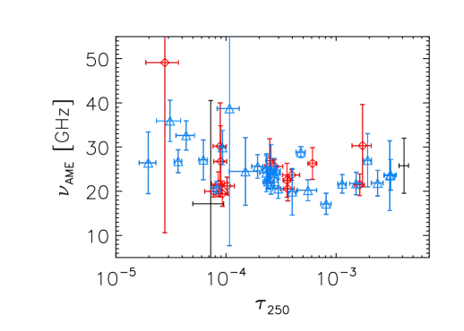
Figure 24: Distribution of the AME peak frequency $\nu_{\rm AME}$ against $\tau_{250}$. All selected data are displayed. Symbols and colours definition are the same as in Figure 9.

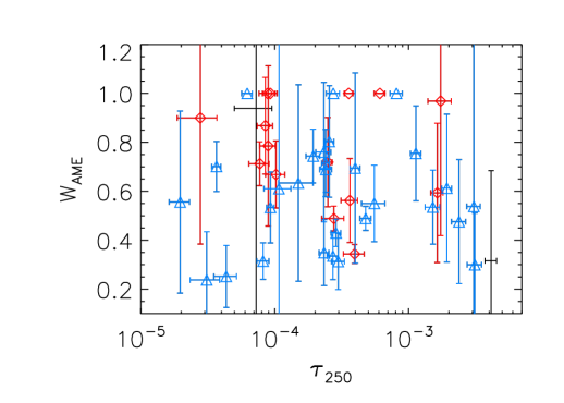
Figure 25: Distribution of the width of the AME $\rm W_{\rm AME}$ against $\tau_{250}$. All selected data are displayed. Symbols and colours definition are the same as in Figure 9.

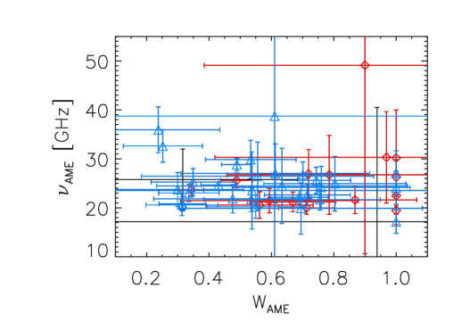
Figure 26: Variations of the AME peak frequency $\nu_{\rm AME}$ as a function of the width of the parabola, $\sigma_{\rm AME,\it\nu}$. Symbols and colours definition are the same as in Figure 9.

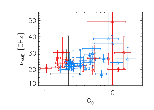
Figure 27: Variations of the AME peak frequency with the relative strength of the ISRF, $G_{0}$. Symbols and colours definition are the same as in Figure 9.

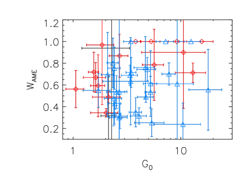
Figure 28: Variations of the AME parabola width parameter with the relative strength of the ISRF, $G_{0}$. Symbols and colours definition are the same as in Figure 9.

Appendix B SED MULTICOMPONENT FIT PARAMETERS

Source Name	$\alpha_{\rm synch,int}$	EM	$\tau_{250}$	$T_{\rm dust}$	$\beta_{\rm dust}$	G0	$\Delta T_{\rm CMB}$
		[cm-6 pc]	[$\times 10^{5}$]	[K]			[$\mu$K]
G010.19-00.32	-0.41 $\pm$ 0.27	1969.0 $\pm$ 86.8	307.0 $\pm$ 35.2	20.6 $\pm$ 0.6	1.90 $\pm$ 0.06	2.68 $\pm$ 0.48	125.0 (PUL)
G010.84-02.59	…	244.2 $\pm$ 17.1	29.8 $\pm$ 3.3	20.7 $\pm$ 0.6	1.68 $\pm$ 0.06	2.73 $\pm$ 0.46	7.3 $\pm$ 20.5
G011.11-00.12	…	2671.4 $\pm$ 111.7	312.3 $\pm$ 38.6	20.6 $\pm$ 0.7	1.88 $\pm$ 0.07	2.67 $\pm$ 0.51	-28.2 $\pm$ 115.6
G012.80-00.19	-0.22 $\pm$ 0.05	1328.8 $\pm$ 118.4	413.0 $\pm$ 41.1	19.9 $\pm$ 0.5	1.92 $\pm$ 0.05	2.13 $\pm$ 0.32	125.0 (PUL)
G015.06-00.69	…	7265.6 $\pm$ 63.8	193.1 $\pm$ 16.6	23.1 $\pm$ 0.5	1.79 $\pm$ 0.04	5.23 $\pm$ 0.74	125.0 (PUL)
G017.00+00.85	…	399.9 $\pm$ 72.9	173.7 $\pm$ 34.3	19.4 $\pm$ 0.9	1.89 $\pm$ 0.12	1.86 $\pm$ 0.53	-74.7 $\pm$ 151.9
G037.79-00.11	-1.33 $\pm$ 0.51	1812.5 $\pm$ 55.6	237.8 $\pm$ 28.9	20.2 $\pm$ 0.6	1.81 $\pm$ 0.07	2.38 $\pm$ 0.44	69.5 $\pm$ 72.9
G040.52+02.53	-0.62 $\pm$ 0.03	6.9 $\pm$ 3.8	25.5 $\pm$ 2.1	20.2 $\pm$ 0.4	1.75 $\pm$ 0.05	2.34 $\pm$ 0.28	69.3 $\pm$ 10.3
G041.03-00.07	-0.80 $\pm$ 0.14	534.3 $\pm$ 34.8	163.6 $\pm$ 17.1	19.1 $\pm$ 0.5	1.83 $\pm$ 0.06	1.71 $\pm$ 0.26	125.0 (PUL)
G043.20-00.10	…	1442.5 $\pm$ 40.2	151.6 $\pm$ 19.0	20.4 $\pm$ 0.7	1.74 $\pm$ 0.07	2.53 $\pm$ 0.48	67.5 $\pm$ 62.3
G045.47+00.06	-1.37 $\pm$ 0.18	383.9 $\pm$ 24.0	113.3 $\pm$ 10.1	20.3 $\pm$ 0.5	1.71 $\pm$ 0.05	2.41 $\pm$ 0.33	125.0 (PUL)
G049.14-00.60	…	3479.9 $\pm$ 35.5	81.1 $\pm$ 8.5	24.3 $\pm$ 0.8	1.72 $\pm$ 0.06	7.22 $\pm$ 1.34	42.2 $\pm$ 38.1
G059.42-00.21	…	286.9 $\pm$ 18.4	55.4 $\pm$ 11.0	19.2 $\pm$ 0.9	1.77 $\pm$ 0.12	1.72 $\pm$ 0.48	-60.4 $\pm$ 29.1
G061.47+00.11	…	311.4 $\pm$ 8.1	23.4 $\pm$ 2.0	21.9 $\pm$ 0.5	1.57 $\pm$ 0.05	3.81 $\pm$ 0.51	8.0 $\pm$ 10.6
G062.98+00.05	…	243.1 $\pm$ 8.2	27.2 $\pm$ 2.7	20.3 $\pm$ 0.5	1.66 $\pm$ 0.06	2.42 $\pm$ 0.37	5.2 $\pm$ 11.4
G070.14+01.61	…	272.4 $\pm$ 26.6	…	10.0 (PLL)	2.11 $\pm$ 2.99	0.03 (PLL)	65.8 $\pm$ 54.9
G071.59+02.85	…	215.4 $\pm$ 17.1	15.0 $\pm$ 4.3	21.5 $\pm$ 1.6	1.57 $\pm$ 0.18	3.42 $\pm$ 1.54	-12.8 $\pm$ 32.9
G075.81+00.39	…	324.7 $\pm$ 12.5	39.9 $\pm$ 3.4	19.8 $\pm$ 0.4	1.65 $\pm$ 0.05	2.09 $\pm$ 0.27	125.0 (PUL)
G076.38-00.62	…	…	11.3 $\pm$ 2.7	24.3 $\pm$ 1.7	1.78 $\pm$ 0.17	7.09 $\pm$ 2.93	56.5 $\pm$ 38.5
G078.57+01.00	…	1835.0 $\pm$ 74.2	32.4 $\pm$ 6.2	23.9 $\pm$ 1.3	1.46 $\pm$ 0.09	6.53 $\pm$ 2.19	-125.0 (PLL)
G081.59+00.01	…	2541.5 $\pm$ 44.1	60.9 $\pm$ 5.6	25.3 $\pm$ 0.7	1.56 $\pm$ 0.04	9.17 $\pm$ 1.54	125.0 (PUL)
G084.68-00.58	…	1201.3 $\pm$ 15.4	35.7 $\pm$ 2.6	21.9 $\pm$ 0.4	1.52 $\pm$ 0.04	3.81 $\pm$ 0.45	-1.3 $\pm$ 23.2
G085.00+04.20	…	435.2 $\pm$ 6.6	9.3 $\pm$ 1.1	23.1 $\pm$ 0.8	1.74 $\pm$ 0.09	5.30 $\pm$ 1.10	86.2 $\pm$ 11.0
G093.02+02.76	…	497.2 $\pm$ 6.6	24.0 $\pm$ 1.6	21.5 $\pm$ 0.4	1.47 $\pm$ 0.04	3.46 $\pm$ 0.37	-19.6 $\pm$ 9.7
G094.47-01.53	…	257.0 $\pm$ 3.7	4.3 $\pm$ 0.8	23.2 $\pm$ 1.2	1.57 $\pm$ 0.13	5.36 $\pm$ 1.64	-6.1 $\pm$ 5.6
G098.00+01.47	…	104.1 $\pm$ 3.5	6.2 $\pm$ 0.6	21.5 $\pm$ 0.5	1.46 $\pm$ 0.05	3.43 $\pm$ 0.50	-20.9 $\pm$ 6.4
G099.60+03.70	…	506.0 $\pm$ 7.6	3.1 $\pm$ 0.8	25.9 $\pm$ 2.0	1.67 $\pm$ 0.17	10.45 $\pm$ 4.80	-34.5 $\pm$ 9.1
G102.88-00.69	…	332.9 $\pm$ 5.9	8.9 $\pm$ 1.2	23.4 $\pm$ 0.9	1.41 $\pm$ 0.08	5.66 $\pm$ 1.25	-83.2 $\pm$ 11.7
G107.20+05.20	…	216.5 $\pm$ 5.6	19.4 $\pm$ 2.3	22.8 $\pm$ 0.8	1.56 $\pm$ 0.06	4.88 $\pm$ 0.97	-1.7 $\pm$ 11.8
G110.25+02.58	…	271.0 $\pm$ 12.9	10.8 $\pm$ 2.4	25.4 $\pm$ 1.7	1.52 $\pm$ 0.13	9.26 $\pm$ 3.81	-52.8 $\pm$ 30.4
G111.54+00.81	…	284.8 $\pm$ 13.8	23.3 $\pm$ 3.0	22.6 $\pm$ 0.8	1.74 $\pm$ 0.08	4.69 $\pm$ 1.02	117.3 $\pm$ 16.2
G118.09+04.96	…	1096.0 $\pm$ 10.6	8.9 $\pm$ 1.2	27.7 $\pm$ 1.3	1.53 $\pm$ 0.08	15.63 $\pm$ 4.30	18.2 $\pm$ 13.0
G123.13-06.27	…	140.4 $\pm$ 1.7	3.7 $\pm$ 0.3	24.6 $\pm$ 0.6	1.34 $\pm$ 0.04	7.76 $\pm$ 1.09	5.5 $\pm$ 3.4
G133.27+09.05	…	…	35.5 $\pm$ 6.1	15.4 $\pm$ 0.6	1.69 $\pm$ 0.09	0.46 $\pm$ 0.10	0.2 $\pm$ 13.1
G133.74+01.22	…	1546.5 $\pm$ 25.3	27.4 $\pm$ 3.1	26.6 $\pm$ 1.0	1.52 $\pm$ 0.06	12.44 $\pm$ 2.77	68.9 $\pm$ 25.9
G142.35+01.35	…	3.1 $\pm$ 2.5	36.4 $\pm$ 5.1	17.7 $\pm$ 0.6	1.67 $\pm$ 0.08	1.06 $\pm$ 0.20	25.6 $\pm$ 13.1
G151.62-00.28	…	311.3 $\pm$ 4.2	9.3 $\pm$ 0.6	23.1 $\pm$ 0.4	1.22 $\pm$ 0.03	5.23 $\pm$ 0.59	-12.5 $\pm$ 7.3
G160.26-18.62	…	46.4 $\pm$ 3.4	27.7 $\pm$ 5.2	19.8 $\pm$ 1.0	1.60 $\pm$ 0.10	2.12 $\pm$ 0.61	19.8 $\pm$ 16.1
G160.60-12.05	…	343.8 $\pm$ 6.4	2.8 $\pm$ 0.9	25.9 $\pm$ 2.6	1.58 $\pm$ 0.20	10.57 $\pm$ 6.25	-35.3 $\pm$ 8.5
G173.56-01.76	…	383.3 $\pm$ 5.9	2.0 $\pm$ 0.3	28.3 $\pm$ 1.6	1.26 $\pm$ 0.10	17.94 $\pm$ 6.07	-26.6 $\pm$ 7.6
G173.62+02.79	…	172.9 $\pm$ 4.3	28.7 $\pm$ 2.4	20.3 $\pm$ 0.5	1.48 $\pm$ 0.04	2.44 $\pm$ 0.33	-26.6 $\pm$ 8.6
G190.00+00.46	…	238.6 $\pm$ 4.7	24.1 $\pm$ 2.5	21.4 $\pm$ 0.6	1.46 $\pm$ 0.05	3.37 $\pm$ 0.58	5.1 $\pm$ 9.5
G192.34-11.37	…	…	11.0 $\pm$ 2.0	18.7 $\pm$ 0.8	1.79 $\pm$ 0.11	1.47 $\pm$ 0.39	12.6 $\pm$ 8.7
G192.60-00.06	…	77.9 $\pm$ 3.1	8.2 $\pm$ 0.9	22.1 $\pm$ 0.6	1.72 $\pm$ 0.07	4.09 $\pm$ 0.70	-13.4 $\pm$ 6.0
G201.62+01.63	…	145.7 $\pm$ 3.5	8.5 $\pm$ 1.1	20.6 $\pm$ 0.7	1.70 $\pm$ 0.09	2.70 $\pm$ 0.53	60.9 $\pm$ 6.4
G203.24+02.08	…	113.4 $\pm$ 3.6	24.9 $\pm$ 1.9	18.8 $\pm$ 0.3	1.53 $\pm$ 0.04	1.56 $\pm$ 0.17	-26.4 $\pm$ 8.1
G208.80-02.65	…	100.5 $\pm$ 6.7	7.3 $\pm$ 2.3	20.1 $\pm$ 1.6	1.59 $\pm$ 0.20	2.28 $\pm$ 1.07	15.5 $\pm$ 19.2
G239.40-04.70	…	63.0 $\pm$ 3.7	10.2 $\pm$ 1.7	19.0 $\pm$ 0.7	1.64 $\pm$ 0.10	1.62 $\pm$ 0.38	9.2 $\pm$ 7.7
G351.31+17.28	…	107.1 $\pm$ 3.1	7.7 $\pm$ 1.3	26.8 $\pm$ 1.4	1.56 $\pm$ 0.10	12.95 $\pm$ 4.05	1.7 $\pm$ 8.2
G353.05+16.90	…	41.5 $\pm$ 4.9	47.8 $\pm$ 4.5	22.7 $\pm$ 0.6	1.57 $\pm$ 0.04	4.75 $\pm$ 0.79	40.9 $\pm$ 12.7
G353.97+15.79	…	28.8 $\pm$ 4.7	39.5 $\pm$ 7.0	19.7 $\pm$ 0.9	1.61 $\pm$ 0.09	2.02 $\pm$ 0.57	-25.4 $\pm$ 17.1
G355.63+20.52	…	…	15.7 $\pm$ 2.8	17.6 $\pm$ 0.7	1.76 $\pm$ 0.11	1.05 $\pm$ 0.26	52.5 $\pm$ 8.1

Table 7: SEDs Fit parameters. ^(PUL): prior upper limit. ^(PLL): prior lower limit.

Source Name	$A_{\rm AME}$	$\sigma_{\rm AME}$	$\nu_{\rm AME}$	$W_{\rm AME}$	$S_{\rm resid}^{28.4}$	$\frac{S_{\rm resid}^{28.4}}{S_{100\mu\rm m}}$	$f_{\rm max}^{\rm UCHII}[15GHz]$	$\chi^{2}_{\rm red}$
	[Jy]		[GHz]	[log[GHz]]	[Jy]
G010.19-00.32	66.7 $\pm$ 26.0	2.6	23.5 $\pm$ 7.9	0.5 $\pm$ 0.7	62.8 $\pm$ 14.2	0.8 $\pm$ 0.2	3.073	0.4
G010.84-02.59	13.3 $\pm$ 2.7	4.8	20.6 $\pm$ 2.2	0.3 $\pm$ 0.1	7.8 $\pm$ 2.6	1.8 $\pm$ 0.7	0.482	0.0
G011.11-00.12	40.6 $\pm$ 16.4	2.5	23.7 $\pm$ 3.5	0.3 $\pm$ 0.2	33.9 $\pm$ 6.8	0.4 $\pm$ 0.1	10.818	0.4
G012.80-00.19	44.0 $\pm$ 36.2	1.2	25.8 $\pm$ 6.2	0.3 $\pm$ 0.4	42.0 $\pm$ 4.5	0.4 $\pm$ 0.1	5.904	0.3
G015.06-00.69	57.7 $\pm$ 7.2	8.0	27.0 $\pm$ 6.0	0.6 $\pm$ 0.3	57.5 $\pm$ 17.0	0.6 $\pm$ 0.2	2.275	0.2
G017.00+00.85	91.8 $\pm$ 15.4	6.0	30.3 $\pm$ 9.3	1.0 $\pm$ 0.5	91.6 $\pm$ 31.7	3.6 $\pm$ 1.4	0.044	0.3
G037.79-00.11	56.0 $\pm$ 7.4	7.6	21.8 $\pm$ 2.9	0.5 $\pm$ 0.3	48.1 $\pm$ 14.0	0.9 $\pm$ 0.3	0.458	0.4
G040.52+02.53	12.5 $\pm$ 1.0	12.9	24.9 $\pm$ 5.6	0.8 $\pm$ 0.2	12.3 $\pm$ 4.1	2.7 $\pm$ 1.0	0.831	0.0
G041.03-00.07	51.8 $\pm$ 6.6	7.9	21.5 $\pm$ 2.5	0.6 $\pm$ 0.3	46.3 $\pm$ 14.0	2.2 $\pm$ 0.8	0.175	0.2
G043.20-00.10	45.7 $\pm$ 5.5	8.3	21.7 $\pm$ 2.5	0.5 $\pm$ 0.2	40.4 $\pm$ 12.0	1.5 $\pm$ 0.5	1.437	0.4
G045.47+00.06	62.4 $\pm$ 4.0	15.6	21.7 $\pm$ 2.1	0.8 $\pm$ 0.2	58.5 $\pm$ 19.3	2.8 $\pm$ 1.1	0.628	0.2
G049.14-00.60	76.2 $\pm$ 3.3	22.9	17.2 $\pm$ 2.4	1.0 (PUL)	67.1 $\pm$ 24.6	1.3 $\pm$ 0.5	1.047	0.2
G059.42-00.21	20.9 $\pm$ 2.4	8.7	20.2 $\pm$ 2.3	0.6 $\pm$ 0.2	17.2 $\pm$ 5.4	2.5 $\pm$ 0.9	0.350	0.7
G061.47+00.11	5.3 $\pm$ 1.3	4.1	25.3 $\pm$ 2.8	0.3 $\pm$ 0.1	5.0 $\pm$ 1.1	0.8 $\pm$ 0.2	10.855	0.1
G062.98+00.05	7.4 $\pm$ 1.2	6.1	23.1 $\pm$ 1.8	0.3 $\pm$ 0.1	6.1 $\pm$ 1.6	1.5 $\pm$ 0.5	1.087	0.2
G070.14+01.61	11.0 $\pm$ 3.6	3.1	23.0 $\pm$ 29.3	1.0 (PUL)	10.8 $\pm$ 3.1	3.8 $\pm$ 1.2	2.820	1.7
G071.59+02.85	12.7 $\pm$ 2.7	4.8	24.5 $\pm$ 7.7	0.6 $\pm$ 0.4	12.4 $\pm$ 3.4	3.0 $\pm$ 1.0	0.007	0.3
G075.81+00.39	19.1 $\pm$ 3.2	5.9	19.9 $\pm$ 5.3	0.7 $\pm$ 0.4	16.8 $\pm$ 5.1	2.6 $\pm$ 0.9	0.575	0.1
G076.38-00.62	15.5 $\pm$ 4.0	3.9	24.5 $\pm$ 14.3	0.9 $\pm$ 0.9	15.2 $\pm$ 4.5	2.3 $\pm$ 0.8	1.195	0.1
G078.57+01.00	…	…	…	…	…	…	…	0.7
G081.59+00.01	94.0 $\pm$ 5.2	17.9	26.3 $\pm$ 3.6	1.0 (PUL)	93.7 $\pm$ 34.3	2.4 $\pm$ 1.0	0.000	0.2
G084.68-00.58	34.6 $\pm$ 1.8	18.8	22.5 $\pm$ 3.8	1.0 (PUL)	33.7 $\pm$ 12.1	3.4 $\pm$ 1.4	0.000	0.1
G085.00+04.20	16.7 $\pm$ 0.8	21.1	19.5 $\pm$ 2.9	1.0 (PUL)	15.5 $\pm$ 5.6	4.8 $\pm$ 1.9	0.010	0.1
G093.02+02.76	13.4 $\pm$ 0.6	21.0	22.6 $\pm$ 2.1	0.7 $\pm$ 0.1	12.7 $\pm$ 4.2	2.3 $\pm$ 0.8	0.724	0.1
G094.47-01.53	2.2 $\pm$ 0.5	4.1	32.6 $\pm$ 3.3	0.3 $\pm$ 0.1	1.9 $\pm$ 0.5	1.4 $\pm$ 0.4	31.097	0.1
G098.00+01.47	10.8 $\pm$ 0.6	17.2	27.1 $\pm$ 4.5	1.0 (PUL)	10.8 $\pm$ 4.0	8.2 $\pm$ 3.4	0.314	0.2
G099.60+03.70	3.0 $\pm$ 1.0	3.0	35.9 $\pm$ 4.7	0.2 $\pm$ 0.2	1.8 $\pm$ 0.6	0.7 $\pm$ 0.2	133.803	0.3
G102.88-00.69	7.5 $\pm$ 0.7	10.9	26.7 $\pm$ 8.1	0.8 $\pm$ 0.3	7.5 $\pm$ 2.5	3.1 $\pm$ 1.1	0.018	0.2
G107.20+05.20	18.5 $\pm$ 0.7	27.8	25.6 $\pm$ 2.7	0.7 $\pm$ 0.1	18.3 $\pm$ 6.1	2.6 $\pm$ 1.0	1.008	0.4
G110.25+02.58	7.6 $\pm$ 2.8	2.7	38.7 $\pm$ 31.0	0.6 $\pm$ 0.6	6.7 $\pm$ 2.1	0.8 $\pm$ 0.3	11.067	0.6
G111.54+00.81	21.4 $\pm$ 2.0	10.8	24.2 $\pm$ 4.3	0.8 $\pm$ 0.3	20.9 $\pm$ 6.7	2.1 $\pm$ 0.8	2.730	0.3
G118.09+04.96	12.9 $\pm$ 0.9	14.2	30.2 $\pm$ 9.8	1.0 (PUL)	12.9 $\pm$ 4.8	1.5 $\pm$ 0.6	0.003	0.3
G123.13-06.27	4.6 $\pm$ 0.2	25.2	26.8 $\pm$ 2.6	0.7 $\pm$ 0.1	4.6 $\pm$ 1.5	3.7 $\pm$ 1.4	0.459	0.1
G133.27+09.05	4.9 $\pm$ 0.4	11.1	21.9 $\pm$ 6.2	0.7 $\pm$ 0.3	4.6 $\pm$ 1.5	8.4 $\pm$ 3.1	0.055	1.3
G133.74+01.22	54.4 $\pm$ 2.2	24.8	24.1 $\pm$ 3.3	1.0 (PUL)	53.7 $\pm$ 19.6	2.3 $\pm$ 0.9	0.553	0.3
G142.35+01.35	6.7 $\pm$ 0.8	8.4	20.6 $\pm$ 2.7	0.6 $\pm$ 0.2	5.7 $\pm$ 1.8	2.4 $\pm$ 0.8	0.200	0.6
G151.62-00.28	5.6 $\pm$ 0.5	11.4	29.9 $\pm$ 3.9	0.5 $\pm$ 0.1	5.6 $\pm$ 1.7	2.7 $\pm$ 0.9	1.301	0.1
G160.26-18.62	14.7 $\pm$ 0.8	19.2	25.6 $\pm$ 1.5	0.5 $\pm$ 0.1	14.4 $\pm$ 4.2	3.2 $\pm$ 1.1	0.064	1.3
G160.60-12.05	9.3 $\pm$ 0.7	12.6	49.1 $\pm$ 38.5	0.9 $\pm$ 0.5	7.7 $\pm$ 3.7	4.1 $\pm$ 2.1	0.000	0.8
G173.56-01.76	2.7 $\pm$ 0.6	4.4	26.4 $\pm$ 7.0	0.6 $\pm$ 0.4	2.7 $\pm$ 0.7	2.1 $\pm$ 0.7	0.055	0.2
G173.62+02.79	9.6 $\pm$ 0.6	15.5	24.7 $\pm$ 1.1	0.4 $\pm$ 0.1	9.1 $\pm$ 2.5	2.6 $\pm$ 0.8	1.631	0.3
G190.00+00.46	14.3 $\pm$ 0.5	29.3	22.2 $\pm$ 1.4	0.7 $\pm$ 0.1	13.4 $\pm$ 4.4	3.1 $\pm$ 1.1	0.848	0.4
G192.34-11.37	9.1 $\pm$ 0.7	12.5	24.9 $\pm$ 4.0	0.7 $\pm$ 0.2	9.0 $\pm$ 2.9	9.1 $\pm$ 3.3	0.000	0.8
G192.60-00.06	3.8 $\pm$ 0.5	7.9	20.8 $\pm$ 1.4	0.3 $\pm$ 0.1	2.4 $\pm$ 0.8	1.0 $\pm$ 0.4	0.719	0.1
G201.62+01.63	10.0 $\pm$ 0.4	27.3	21.6 $\pm$ 2.8	0.9 $\pm$ 0.2	9.5 $\pm$ 3.3	6.5 $\pm$ 2.5	0.056	0.1
G203.24+02.08	7.1 $\pm$ 0.4	15.8	26.9 $\pm$ 5.0	0.7 $\pm$ 0.2	7.1 $\pm$ 2.3	3.6 $\pm$ 1.3	0.022	0.2
G208.80-02.65	3.4 $\pm$ 1.8	1.9	17.2 $\pm$ 23.4	0.9 $\pm$ 1.7	3.0 $\pm$ 0.7	4.3 $\pm$ 1.2	0.025	0.2
G239.40-04.70	6.9 $\pm$ 0.4	16.5	21.2 $\pm$ 2.0	0.7 $\pm$ 0.1	6.3 $\pm$ 2.1	6.9 $\pm$ 2.5	0.000	0.3
G351.31+17.28	12.0 $\pm$ 0.4	32.9	20.0 $\pm$ 1.3	0.7 $\pm$ 0.1	10.6 $\pm$ 3.6	1.5 $\pm$ 0.6	0.036	0.1
G353.05+16.90	20.0 $\pm$ 0.7	27.3	28.8 $\pm$ 1.2	0.5 $\pm$ 0.1	20.0 $\pm$ 6.0	1.3 $\pm$ 0.5	0.997	0.4
G353.97+15.79	13.1 $\pm$ 1.2	10.6	23.7 $\pm$ 1.2	0.3 $\pm$ 0.1	11.4 $\pm$ 3.1	3.5 $\pm$ 1.1	0.190	0.3
G355.63+20.52	8.1 $\pm$ 0.5	17.0	23.5 $\pm$ 1.2	0.5 $\pm$ 0.1	7.5 $\pm$ 2.2	7.7 $\pm$ 2.6	0.000	0.7

Table 8: SEDs Fit parameters. ^(PUL): prior upper limit.

The parameters obtained on each source from the multicomponent analysis are displayed in Table 7 and Table 8. The name of the sources are given in column one from each Table. The parameters used to model the synchrotron component, and the free-free component, are given in columns 2 and 3 from Table 7, respectively. Columns 4 to 6 of the same table give the parameters used to model the thermal dust grain component, while column 7 gives the relative strength of the ISRF derived using $T_{\rm dust}$ displayed in column 5. The parameter used to model the CMB component is found in the last column of Table 7. All the parameters related to the modelling of AME are given in Table 8. The maximum fraction of emission that could be attributed to UCH ii regions is given in column 8 of that table, while the reduced $\chi^{2}$ of the multicomponent fits are given in the last column.

Appendix C SEDs of the full sample

The plots of the SEDs obtained on each of the 52 candidate AME sources of the sample are displayed in Figures C1–C7. In each plot, the QUIJOTE intensity flux densities are shown with red filled circles, and the WMAP, Planck, and DIRBE intensity flux densities are shown with green, blue, and yellow opened diamonds, respectively. The low frequency points used to fit the models are shown in pale blue, and in blue if they were not included in the fitting procedure. The result of the multicomponent fit is illustrated by the continuous black curve. The fit to the AME component is shown with the dashed red line. The fit to the free–free component is shown with the dashed blue line. The fit to the thermal dust component is shown with the dashed yellow line. The fit to the CMB component is shown with the dashed green line.

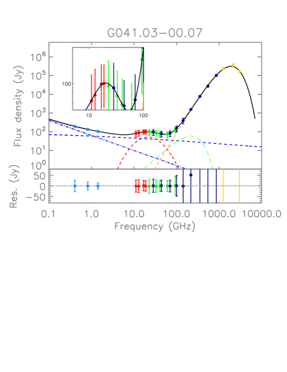
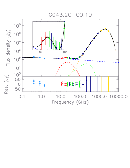
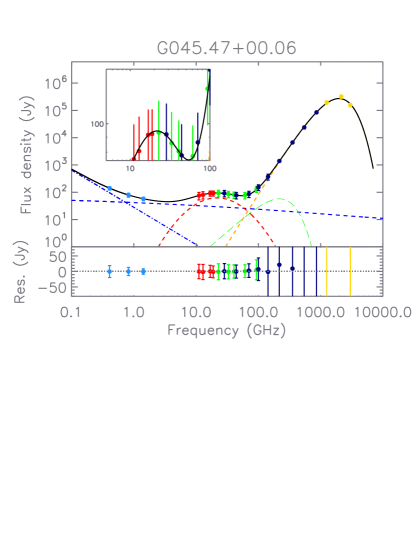
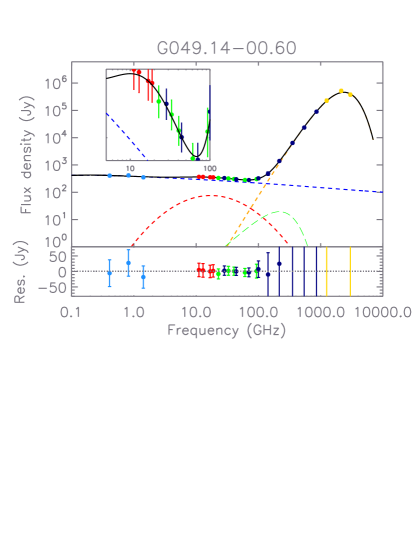
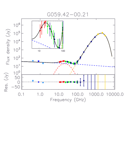
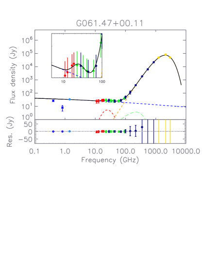
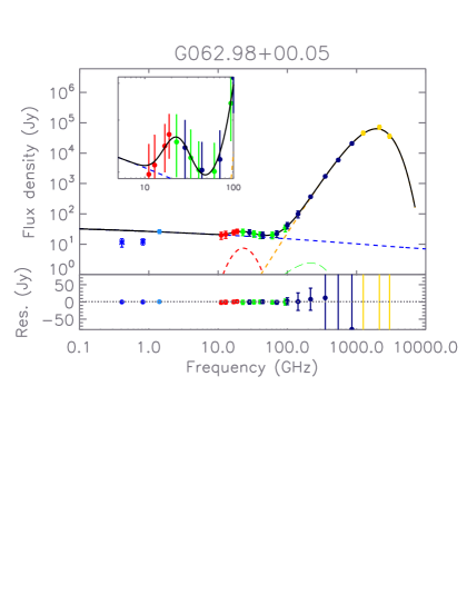
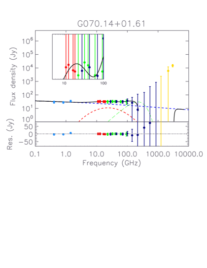
Figure 30: Same as Figure 29.

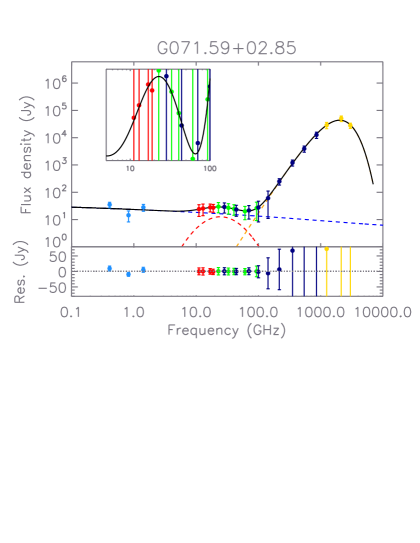
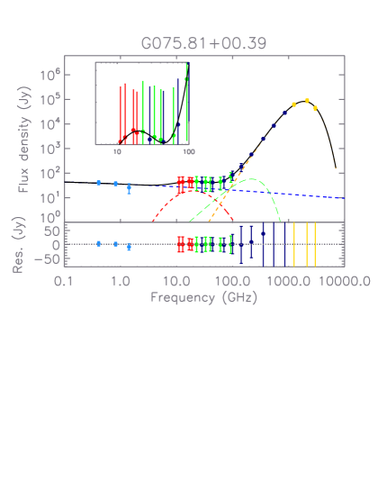
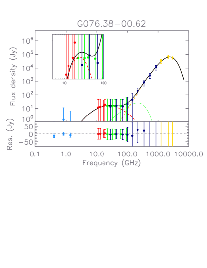
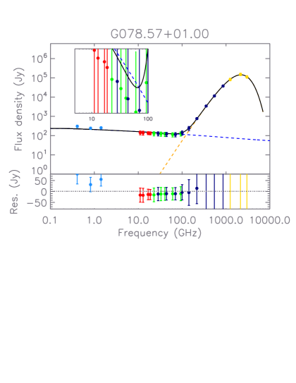
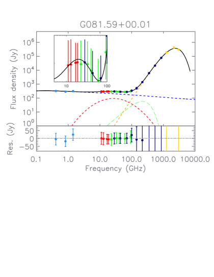
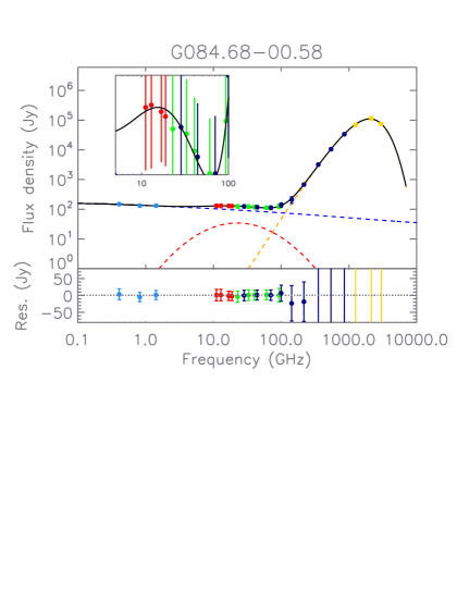
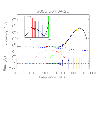
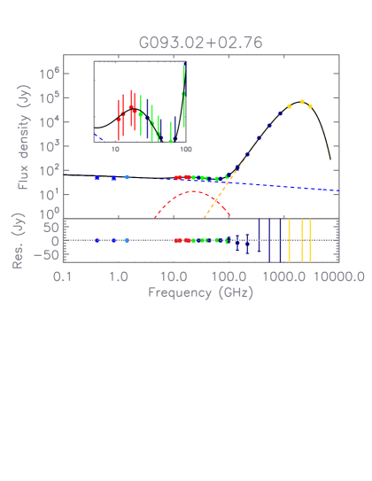
Figure 31: Same as Figure 29.

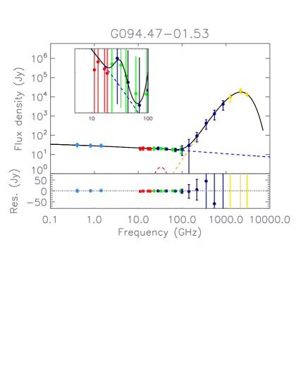
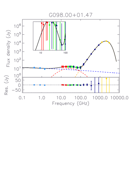
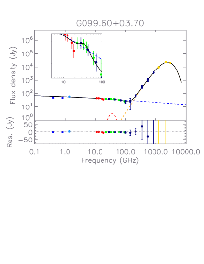
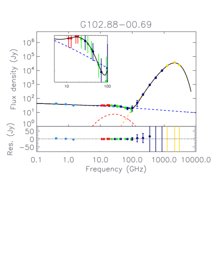
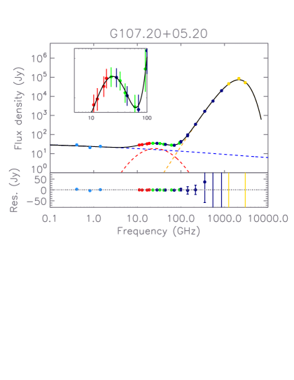
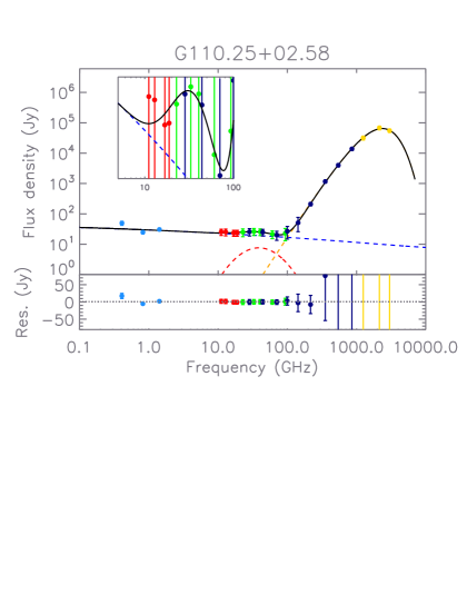
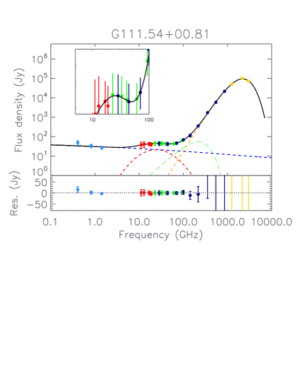
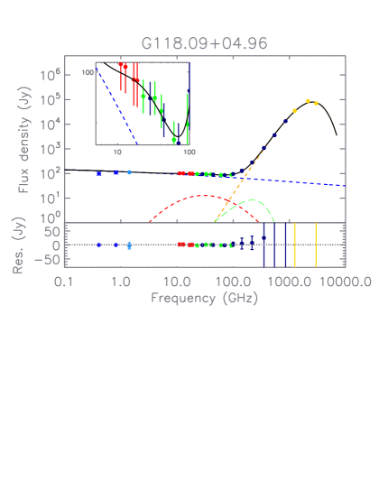
Figure 32: Same as Figure 29.

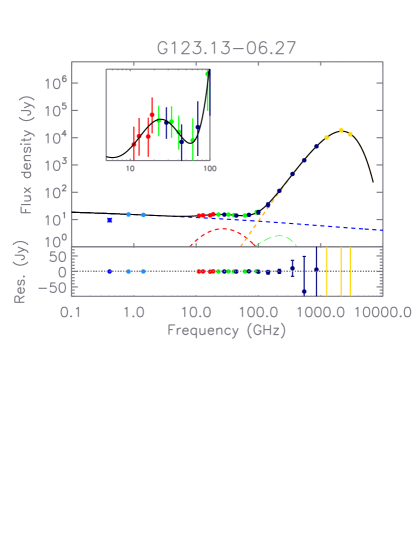
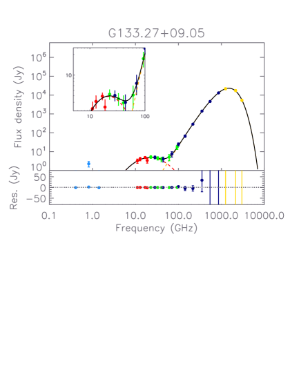
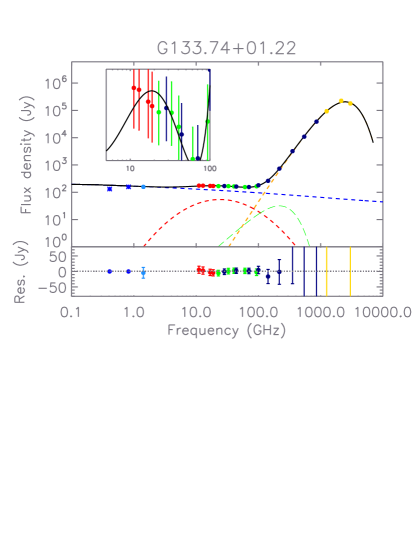
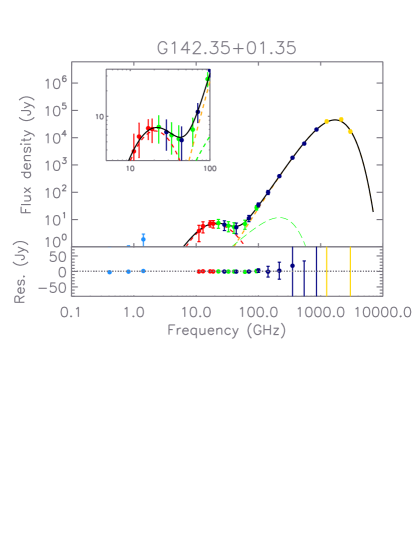
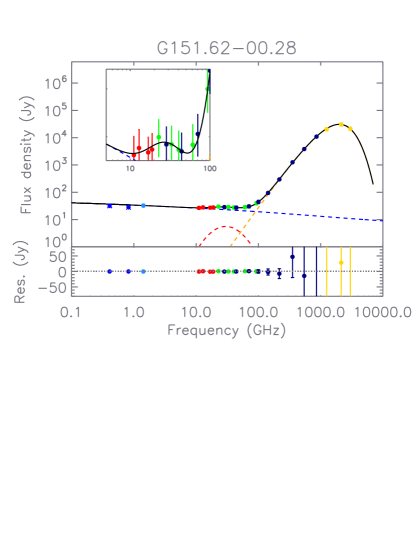
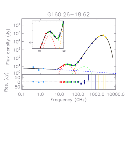
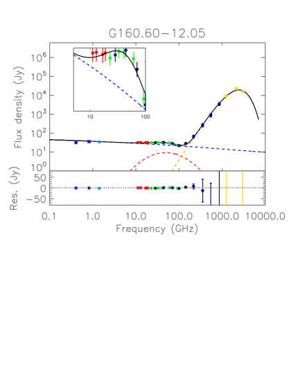
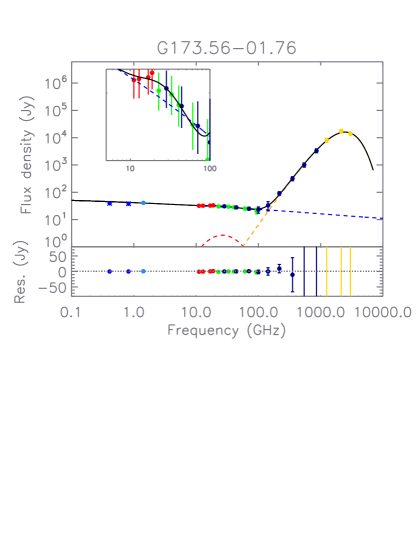
Figure 33: Same as Figure 29.

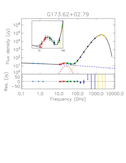
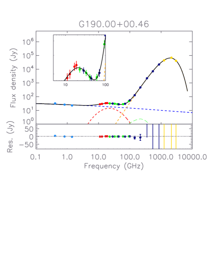
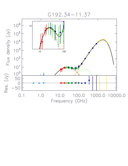
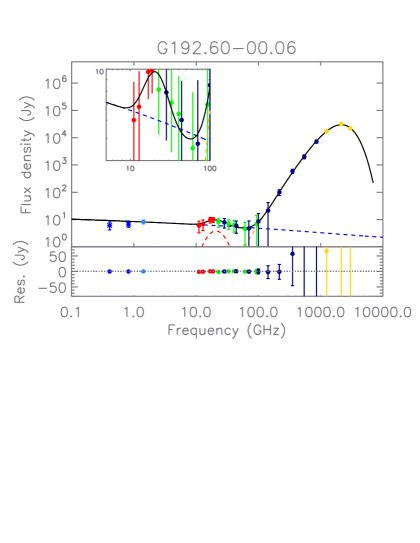
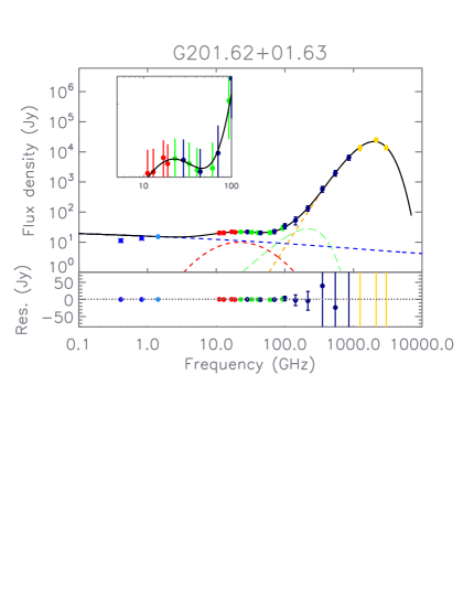
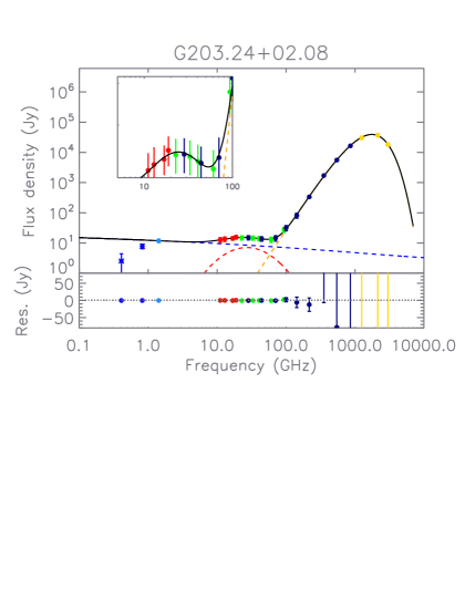
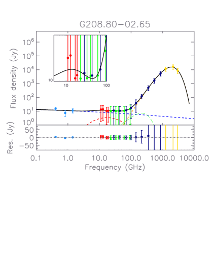
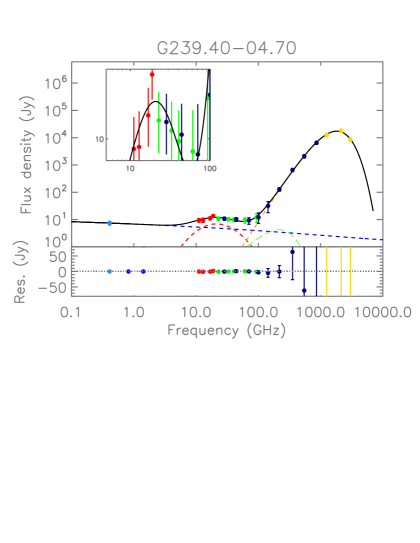
Figure 34: Same as Figure 29.

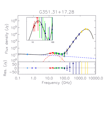
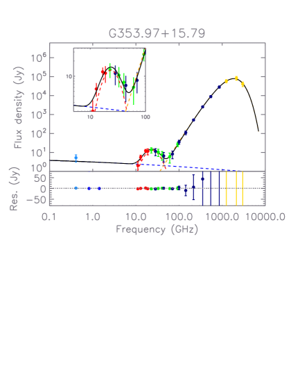
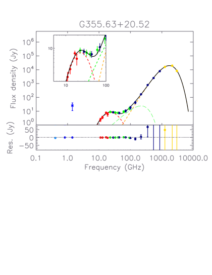
Figure 35: Same as Figure 29.

Appendix D Additional TABLES

All the SRCCs obtained between the several parameters used to model the free-free, AME, and thermal dust components are displayed in Tables D1–D5. In additional to several plots used to study correlations between some of the parameters, these tables have been used to systematically identify the parameters showing the most meaningful correlation factors, and guide our study.

Variable 1	Variable 2	SRCC	SRCC	SRCC
		selected sample	AME significant	AME semi-significant
$A_{\rm AME}[\rm Jy]$	$\nu_{\rm AME}[\rm GHz]$	$-$0.20$\pm$ 0.11	0.10$\pm$ 0.22	$-$0.52$\pm$ 0.13
$A_{\rm AME}[\rm Jy]$	$W_{\rm AME}$	0.27$\pm$ 0.12	0.39$\pm$ 0.20	0.40$\pm$ 0.14
$A_{\rm AME}[\rm Jy]$	$A_{\rm AME}/\tau_{250}[\rm Jy]$	$-$0.11$\pm$ 0.08	0.19$\pm$ 0.09	$-$0.27$\pm$ 0.10
$A_{\rm AME}[\rm Jy]$	$\Re_{\rm AME}$	0.88$\pm$ 0.15	0.77$\pm$ 0.27	0.91$\pm$ 0.22
$\nu_{\rm AME}[\rm GHz]$	$W_{\rm AME}$	$-$0.06$\pm$ 0.14	0.27$\pm$ 0.26	$-$0.12$\pm$ 0.17
$\nu_{\rm AME}[\rm GHz]$	$A_{\rm AME}/\tau_{250}[\rm Jy]$	0.18$\pm$ 0.13	0.02$\pm$ 0.22	0.31$\pm$ 0.16
$\nu_{\rm AME}[\rm GHz]$	$\Re_{\rm AME}$	$-$0.04$\pm$ 0.15	0.34$\pm$ 0.25	$-$0.33$\pm$ 0.20
$W_{\rm AME}$	$A_{\rm AME}/\tau_{250}[\rm Jy]$	0.66$\pm$ 0.12	0.64$\pm$ 0.18	0.57$\pm$ 0.15
$W_{\rm AME}$	$\Re_{\rm AME}$	0.60$\pm$ 0.15	0.75$\pm$ 0.27	0.67$\pm$ 0.20
$A_{\rm AME}/\tau_{250}[\rm Jy]$	$\Re_{\rm AME}$	0.19$\pm$ 0.15	0.43$\pm$ 0.26	$-$0.01$\pm$ 0.19

Table 9: Spearman rank correlation coefficients (SRCCs) between AME and AME parameters.

Variable 1	Variable 2	SRCC	SRCC	SRCC
		selected sample	AME significant	AME semi-significant
$A_{\rm AME}[\rm Jy]$	Ttd or $G_{0}$	$-$0.16$\pm$ 0.06	0.26$\pm$ 0.10	$-$0.33$\pm$ 0.07
$A_{\rm AME}[\rm Jy]$	$\beta_{\rm td}$	0.49$\pm$ 0.08	0.21$\pm$ 0.14	0.56$\pm$ 0.09
$A_{\rm AME}[\rm Jy]$	$\tau_{250}$	0.81$\pm$ 0.04	0.53$\pm$ 0.07	0.85$\pm$ 0.04
$A_{\rm AME}[\rm Jy]$	$S_{\rm TD,peak}[\rm Jy]$	0.88$\pm$ 0.05	0.82$\pm$ 0.07	0.91$\pm$ 0.04
$A_{\rm AME}[\rm Jy]$	$\nu_{\rm TD,peak}[\rm GHz]$	0.04$\pm$ 0.11	0.34$\pm$ 0.17	$-$0.07$\pm$ 0.15
$A_{\rm AME}[\rm Jy]$	$\Re_{\rm td}x10^{-4}$	0.88$\pm$ 0.05	0.85$\pm$ 0.08	0.90$\pm$ 0.05
$\nu_{\rm AME}[\rm GHz]$	Ttd or $G_{0}$	0.40$\pm$ 0.12	0.21$\pm$ 0.22	0.60$\pm$ 0.15
$\nu_{\rm AME}[\rm GHz]$	$\beta_{\rm td}$	$-$0.35$\pm$ 0.13	$-$0.35$\pm$ 0.26	$-$0.44$\pm$ 0.16
$\nu_{\rm AME}[\rm GHz]$	$\tau_{250}$	$-$0.25$\pm$ 0.12	0.01$\pm$ 0.23	$-$0.57$\pm$ 0.14
$\nu_{\rm AME}[\rm GHz]$	$S_{\rm TD,peak}[\rm Jy]$	$-$0.14$\pm$ 0.13	0.11$\pm$ 0.23	$-$0.47$\pm$ 0.14
$\nu_{\rm AME}[\rm GHz]$	$\nu_{\rm TD,peak}[\rm GHz]$	0.34$\pm$ 0.13	0.19$\pm$ 0.23	0.42$\pm$ 0.17
$\nu_{\rm AME}[\rm GHz]$	$\Re_{\rm td}x10^{-4}$	$-$0.11$\pm$ 0.13	0.11$\pm$ 0.21	$-$0.42$\pm$ 0.14
$W_{\rm AME}$	Ttd or $G_{0}$	0.23$\pm$ 0.12	0.57$\pm$ 0.18	0.07$\pm$ 0.15
$W_{\rm AME}$	$\beta_{\rm td}$	$-$0.24$\pm$ 0.13	$-$0.23$\pm$ 0.25	$-$0.21$\pm$ 0.16
$W_{\rm AME}$	$\tau_{250}$	$-$0.17$\pm$ 0.12	$-$0.18$\pm$ 0.23	$-$0.00$\pm$ 0.16
$W_{\rm AME}$	$S_{\rm TD,peak}[\rm Jy]$	$-$0.05$\pm$ 0.12	0.22$\pm$ 0.22	0.08$\pm$ 0.15
$W_{\rm AME}$	$\nu_{\rm TD,peak}[\rm GHz]$	0.18$\pm$ 0.13	0.68$\pm$ 0.19	0.00$\pm$ 0.17
$W_{\rm AME}$	$\Re_{\rm td}x10^{-4}$	$-$0.01$\pm$ 0.12	0.28$\pm$ 0.22	0.12$\pm$ 0.15
$A_{\rm AME}/\tau_{250}[\rm Jy]$	Ttd or $G_{0}$	0.68$\pm$ 0.08	0.87$\pm$ 0.07	0.62$\pm$ 0.11
$A_{\rm AME}/\tau_{250}[\rm Jy]$	$\beta_{\rm td}$	$-$0.52$\pm$ 0.09	$-$0.20$\pm$ 0.20	$-$0.64$\pm$ 0.10
$A_{\rm AME}/\tau_{250}[\rm Jy]$	$\tau_{250}$	$-$0.64$\pm$ 0.08	$-$0.64$\pm$ 0.09	$-$0.68$\pm$ 0.10
$A_{\rm AME}/\tau_{250}[\rm Jy]$	$S_{\rm TD,peak}[\rm Jy]$	$-$0.41$\pm$ 0.08	$-$0.13$\pm$ 0.13	$-$0.54$\pm$ 0.09
$A_{\rm AME}/\tau_{250}[\rm Jy]$	$\nu_{\rm TD,peak}[\rm GHz]$	0.54$\pm$ 0.11	0.88$\pm$ 0.12	0.40$\pm$ 0.15
$A_{\rm AME}/\tau_{250}[\rm Jy]$	$\Re_{\rm td}x10^{-4}$	$-$0.34$\pm$ 0.09	$-$0.01$\pm$ 0.15	$-$0.48$\pm$ 0.10
$\Re_{\rm AME}$	Ttd or $G_{0}$	0.04$\pm$ 0.16	0.45$\pm$ 0.27	$-$0.20$\pm$ 0.20
$\Re_{\rm AME}$	$\beta_{\rm td}$	0.31$\pm$ 0.14	0.05$\pm$ 0.26	0.36$\pm$ 0.18
$\Re_{\rm AME}$	$\tau_{250}$	0.54$\pm$ 0.14	0.19$\pm$ 0.23	0.65$\pm$ 0.17
$\Re_{\rm AME}$	$S_{\rm TD,peak}[\rm Jy]$	0.68$\pm$ 0.14	0.60$\pm$ 0.24	0.72$\pm$ 0.16
$\Re_{\rm AME}$	$\nu_{\rm TD,peak}[\rm GHz]$	0.20$\pm$ 0.16	0.60$\pm$ 0.28	$-$0.01$\pm$ 0.20
$\Re_{\rm AME}$	$\Re_{\rm td}x10^{-4}$	0.70$\pm$ 0.14	0.66$\pm$ 0.23	0.73$\pm$ 0.17

Table 10: Spearman rank correlation coefficients (SRCCs) between AME and Thermal Dust parameters.

Variable 1	Variable 2	SRCC	SRCC	SRCC
		selected sample	AME significant	free-free semi-significant
$A_{\rm AME}[\rm Jy]$	EM [cm${}^{-6}/$pc]	0.59$\pm$ 0.04	0.65$\pm$ 0.11	0.55$\pm$ 0.03
$\nu_{\rm AME}[\rm GHz]$	EM [cm${}^{-6}/$pc]	0.06$\pm$ 0.11	0.27$\pm$ 0.20	$-$0.24$\pm$ 0.14
$W_{\rm AME}$	EM [cm${}^{-6}/$pc]	0.12$\pm$ 0.10	0.84$\pm$ 0.13	$-$0.02$\pm$ 0.14
$A_{\rm AME}/\tau_{250}[\rm Jy]$	EM [cm${}^{-6}/$pc]	0.01$\pm$ 0.07	0.46$\pm$ 0.14	$-$0.21$\pm$ 0.07
$\Re_{\rm AME}$	EM [cm${}^{-6}/$pc]	0.59$\pm$ 0.14	0.90$\pm$ 0.24	0.42$\pm$ 0.17

Table 11: Spearman rank correlation coefficients (SRCCs) between AME and free-free parameters.

Variable 1	Variable 2	SRCC	SRCC	SRCC
		selected sample	AME significant	free-free semi-significant
Ttd or $G_{0}$	EM [cm${}^{-6}/$pc]	0.30$\pm$ 0.06	0.49$\pm$ 0.13	0.09$\pm$ 0.07
$\beta_{\rm td}$	EM [cm${}^{-6}/$pc]	0.28$\pm$ 0.07	$-$0.17$\pm$ 0.16	0.41$\pm$ 0.07
$\tau_{250}$	EM [cm${}^{-6}/$pc]	0.43$\pm$ 0.03	0.10$\pm$ 0.09	0.51$\pm$ 0.03
$S_{\rm TD,peak}[\rm Jy]$	EM [cm${}^{-6}/$pc]	0.64$\pm$ 0.03	0.50$\pm$ 0.08	0.64$\pm$ 0.04
$\nu_{\rm TD,peak}[\rm GHz]$	EM [cm${}^{-6}/$pc]	0.45$\pm$ 0.10	0.62$\pm$ 0.17	0.29$\pm$ 0.15
$\Re_{\rm td}x10^{-4}$	EM [cm${}^{-6}/$pc]	0.66$\pm$ 0.04	0.56$\pm$ 0.09	0.65$\pm$ 0.04

Table 12: Spearman rank correlation coefficients (SRCCs) between thermal dust and free-free parameters.

Variable 1	Variable 2	SRCC	SRCC	SRCC
		selected sample	AME significant	AME semi-significant
Ttd or $G_{0}$	$\beta_{\rm td}$	$-$0.47$\pm$ 0.09	$-$0.44$\pm$ 0.18	$-$0.47$\pm$ 0.10
Ttd or $G_{0}$	$\tau_{250}$	$-$0.52$\pm$ 0.05	$-$0.57$\pm$ 0.10	$-$0.58$\pm$ 0.07
Ttd or $G_{0}$	$S_{\rm TD,peak}[\rm Jy]$	$-$0.17$\pm$ 0.07	0.11$\pm$ 0.14	$-$0.32$\pm$ 0.08
Ttd or $G_{0}$	$\nu_{\rm TD,peak}[\rm GHz]$	0.92$\pm$ 0.08	0.97$\pm$ 0.12	0.85$\pm$ 0.13
Ttd or $G_{0}$	$\Re_{\rm td}x10^{-4}$	$-$0.07$\pm$ 0.07	0.22$\pm$ 0.14	$-$0.25$\pm$ 0.09
$\beta_{\rm td}$	$\tau_{250}$	0.60$\pm$ 0.08	0.34$\pm$ 0.18	0.69$\pm$ 0.09
$\beta_{\rm td}$	$S_{\rm TD,peak}[\rm Jy]$	0.54$\pm$ 0.08	0.06$\pm$ 0.17	0.68$\pm$ 0.09
$\beta_{\rm td}$	$\nu_{\rm TD,peak}[\rm GHz]$	$-$0.13$\pm$ 0.12	$-$0.31$\pm$ 0.22	0.01$\pm$ 0.16
$\beta_{\rm td}$	$\Re_{\rm td}x10^{-4}$	0.50$\pm$ 0.08	0.03$\pm$ 0.17	0.65$\pm$ 0.09
$\tau_{250}$	$S_{\rm TD,peak}[\rm Jy]$	0.90$\pm$ 0.04	0.69$\pm$ 0.10	0.92$\pm$ 0.04
$\tau_{250}$	$\nu_{\rm TD,peak}[\rm GHz]$	$-$0.31$\pm$ 0.11	$-$0.51$\pm$ 0.16	$-$0.29$\pm$ 0.14
$\tau_{250}$	$\Re_{\rm td}x10^{-4}$	0.85$\pm$ 0.05	0.61$\pm$ 0.13	0.88$\pm$ 0.05
$S_{\rm TD,peak}[\rm Jy]$	$\nu_{\rm TD,peak}[\rm GHz]$	0.06$\pm$ 0.12	0.18$\pm$ 0.19	$-$0.01$\pm$ 0.15
$S_{\rm TD,peak}[\rm Jy]$	$\Re_{\rm td}x10^{-4}$	0.99$\pm$ 0.05	0.99$\pm$ 0.11	0.99$\pm$ 0.05
$\nu_{\rm TD,peak}[\rm GHz]$	$\Re_{\rm td}x10^{-4}$	0.17$\pm$ 0.12	0.30$\pm$ 0.19	0.06$\pm$ 0.15

Table 13: Spearman rank correlation coefficients (SRCCs) between the thermal dust parameters.

References

- Aiola et al. (2020) Aiola S., et al., 2020, J. Cosmology Astropart. Phys., 2020, 047
- Ali-Haimoud (2010) Ali-Haimoud Y., 2010, SpDust/SpDust.2: Code to Calculate Spinning Dust Spectra (ascl:1010.016)
- Ali-Haïmoud et al. (2009) Ali-Haïmoud Y., Hirata C. M., Dickinson C., 2009, MNRAS, 395, 1055
- Arce-Tord et al. (2020) Arce-Tord C., et al., 2020, MNRAS, 495, 3482
- BICEP/Keck collaboration et al. (2021) BICEP/Keck collaboration et al., 2021, Phys. Rev. Lett., 127, 151301
- Battistelli et al. (2019) Battistelli E. S., et al., 2019, ApJ, 877, L31
- Bell et al. (2019) Bell A. C., Onaka T., Galliano F., Wu R., Doi Y., Kaneda H., Ishihara D., Giard M., 2019, PASJ, 71, 123
- Bennett et al. (2013) Bennett C. L., et al., 2013, ApJS, 208, 20
- Berkhuijsen (1972) Berkhuijsen E. M., 1972, A&AS, 5, 263
- Bernstein et al. (2020) Bernstein L. S., Shroll R. M., Quenneville J., Dickinson C., 2020, ApJ, 892, 69
- Bertin & Arnouts (1996) Bertin E., Arnouts S., 1996, A&AS, 117, 393
- Bonaldi et al. (2007) Bonaldi A., Ricciardi S., Leach S., Stivoli F., Baccigalupi C., de Zotti G., 2007, MNRAS, 382, 1791
- Boulanger et al. (1988) Boulanger F., Beichman C., Desert F. X., Helou G., Perault M., Ryter C., 1988, ApJ, 332, 328
- Carretti et al. (2019) Carretti E., et al., 2019, MNRAS, 489, 2330
- Casassus et al. (2006) Casassus S., Cabrera G. F., Förster F., Pearson T. J., Readhead A. C. S., Dickinson C., 2006, ApJ, 639, 951
- Casassus et al. (2008) Casassus S., et al., 2008, MNRAS, 391, 1075
- Casassus et al. (2021) Casassus S., Vidal M., Arce-Tord C., Dickinson C., White G. J., Burton M., Indermuehle B., Hensley B., 2021, MNRAS,