QUIJOTE scientific results – V. The microwave intensity and polarisation spectra of the Galactic regions W49, W51 and IC443

Abstract

We present new intensity and polarisation maps obtained with the QUIJOTE experiment towards the Galactic regions W49, W51 and IC443, covering the frequency range from 10 to 20 GHz at $\sim 1\,\text{deg}$ angular resolution, with a sensitivity in the range 35–79 $\mu\text{K}\,\text{beam}^{-1}$ for total intensity and 13–23 $\mu\text{K}\,\text{beam}^{-1}$ for polarisation. For each region, we combine QUIJOTE maps with ancillary data at frequencies ranging from 0.4 to 3000 GHz, reconstruct the spectral energy distribution and model it with a combination of known foregrounds. We detect anomalous microwave emission (AME) in total intensity towards W49 at $4.7\sigma$ and W51 at $4.0\sigma$ with peak frequencies $\nu_{\rm AME}=(20.0\pm 1.4)\,\text{GHz}$ and $\nu_{\rm AME}=(17.7\pm 3.6)\,\text{GHz}$ respectively; this is the first detection of AME towards W51. The contamination from ultra-compact HII regions to the residual AME flux density is estimated at 10% in W49 and 5% in W51, and does not rule out the AME detection. The polarised SEDs reveal a synchrotron contribution with spectral indices $\alpha_{\rm s}=-0.67\pm 0.10$ in W49 and $\alpha_{\rm s}=-0.51\pm 0.07$ in W51, ascribed to the diffuse Galactic emission and to the local supernova remnant respectively. Towards IC443 in total intensity we measure a broken power-law synchrotron spectrum with cut-off frequency $\nu_{\rm 0,s}=(114\pm 73)\,\text{GHz}$, in agreement with previous studies; our analysis, however, rules out any AME contribution which had been previously claimed towards IC443. No evidence of polarised AME emission is detected in this study.

1 Introduction

During the past two decades the study of the cosmic microwave background (CMB) anisotropies allowed to estimate cosmological parameters to the per cent precision level, and led to the establishment of the Lambda-Cold Dark Matter ($\Lambda$CDM) cosmology as the most widely accepted paradigm describing our Universe (Hinshaw et al., 2013; Planck Collaboration et al., 2020a). The most recent endeavors are focussing on the characterisation of CMB polarisation, in particular on the search for the inflationary B-mode anisotropies (Kamionkowski et al., 1997; Zaldarriaga & Seljak, 1997). However, to date only upper limits on the level of primordial B-modes anisotropies are available (Planck Collaboration et al., 2020b; BICEP/Keck Collaboration et al., 2021; Ade et al., 2021), as this signal is subdominant compared to other polarised Galactic and extra-Galactic emissions. An accurate modelling of these foregrounds becomes then of paramount importance, not only to produce clean CMB maps for their cosmological exploitation, but also to better characterise the physical properties of the interstellar medium (ISM).

In total intensity, the main foregrounds affecting any CMB observations are synchtrotron radiation generated by cosmic ray electrons spiralling in the Galactic magnetic field, free-free emission from electron thermal bremsstrahlung, thermal radiation from insterstellar dust, and the so-called anomalous microwave emission (AME, Planck Collaboration et al., 2016c); to this list of continuum emissions we can also add the contamination from molecular lines (mostly CO). While the mechanisms responsible for the first three continuum foregrounds are physically well understood, the nature of AME is still under debate (for a detailed review we redirect to Dickinson et al., 2018). This emission, first discovered in the mid-90s (Leitch et al., 1997), appears at frequencies $\sim$10–60 GHz as a dust-correlated signal that cannot be explained in terms of the other foreground components. The most accredited model explaining its origin is the dipole radiation from small, fast spinning dust grains in the ISM (Draine & Lazarian, 1998; Ali-Haïmoud et al., 2009; Hoang et al., 2010; Ysard & Verstraete, 2010; Silsbee et al., 2011; Ali-Haïmoud, 2013); this scenario is referred to as spinning dust emission (SDE). A different model known as magnetic dust emission (MDE) has also been proposed, according to which the thermal emission from magnetised ISM dust grains is the mechanism responsible for AME (Draine & Lazarian, 1999; Draine & Hensley, 2013). More recently, models based on thermal emission from amorphous dust grains proved effective in yielding the excess AME signal at microwave frequencies (Nashimoto et al., 2020). Many observational efforts have tackled the detection of AME in the attempt of better characterising its nature (de Oliveira-Costa et al., 1998; de Oliveira-Costa et al., 1999; Finkbeiner et al., 2002; Watson et al., 2005; Casassus et al., 2006; Davies et al., 2006; AMI Consortium et al., 2009; Dickinson et al., 2009; Murphy et al., 2010; Tibbs et al., 2010; Planck Collaboration et al., 2011; Vidal et al., 2011; Génova-Santos et al., 2011; Planck Collaboration et al., 2014a; Battistelli et al., 2015; Vidal et al., 2020). However, up to date the results are not clear; a promising way of distinguishing between different AME models is the observation of its polarisation.

Out of the aforementioned foregrounds, the free-free emission is known to be practically unpolarised (Rybicki & Lightman, 1979; Trujillo-Bueno et al., 2002), whereas synchrotron and thermal dust emissions yield respectively polarisation fractions $\Pi$ up to 40% and 20% in some regions of the sky (Kogut et al., 2007; Vidal et al., 2015; Planck Collaboration et al., 2016c; Planck Collaboration et al., 2020c; Planck Collaboration et al., 2020d). On the contrary, the polarisation properties of AME are still under debate. Theoretically, predictions have been made for the spinning dust model; although the dipole emission from an individual dust grain is expected to be linearly polarised, the presence of a detectable polarisation fraction in the observed SDE strongly depends on the spatial alignment of ISM grains. Studies of the conditions for grain alignment have been addressed in the literature (Lazarian & Draine, 2000; Hoang et al., 2013) and generally place upper limits for the SDE polarisation fraction at the per cent level. The work by Draine & Hensley (2016), however, suggests that at $\nu\gtrsim 10\,\text{GHz}$ quantum effects prevent the dissipation of the grain rotational energy, thereby erasing the alignment and resulting in negligible polarisation levels ($\Pi\ll 1\%$). The theoretical study of MDE polarisation has also been tackled: Draine & Lazarian (1999) and Draine & Hensley (2013) found that in the case of free-flying magnetized grains the resulting polarisation fraction can be as high as 30%; a more recent study described in Hoang & Lazarian (2016), however, set the upper limits for the polarised emission fraction from free-flying iron nanoparticles at $\sim 5\%$. Similar constraints were obtained in the case of magnetic inclusions within larger, non-magnetic grains (Draine & Hensley, 2013). The MDE is then expected to provide higher polarisation fractions compared to the SDE scenario. The amorphous dust models, finally, found that the AME polarisation is suppressed by the contribution from amorphous carbon dust, accounting for nearly half of the ISM grains (Nashimoto et al., 2020).

Observationally, there are no clear detections of AME in polarisation to date yet. Polarised AME has been searched for with dedicated observations towards a number of different environments, such as supernova remnants (SNRs), planetary nebulae or molecular clouds (Rubiño-Martín et al., 2012a). Battistelli et al. (2006) reported a tentative detection towards the Perseus molecular complex using the COSMOlogical Structures On Medium Angular Scales (COSMOSOMAS) experiment, with an observed polarisation fraction at $\Pi=3.4^{+1.5}_{-1.9}\%$ that could be proceeding from AME. Other works employing different facilites only determined upper limits, usually in the range $\Pi\lesssim 1$–6%  (Casassus et al., 2008; Mason et al., 2009; Macellari et al., 2011; López-Caraballo et al., 2011; Dickinson et al., 2011; Battistelli et al., 2015). These constraints agree in the observed lack of a strong polarised AME component, but are still too loose to clearly discriminate between the different AME models.

Table 1: Summary of the three sources considered in this study. For each one we report the effective central Galactic coordinates $(l_{\rm c},b_{\rm c})$, the possible substructures, the diametral angular size, the estimated distance and the age of the associated SNR. The last three columns quote the relevant quantities for the aperture photometry analysis described in Section 5, namely the radii of the chosen aperture ($r_{\rm ap}$) and of the internal ($r_{\rm int}$) and external ($r_{\rm ext}$) boundaries of the background annulus.

Source	($l_{\rm c}$,$b_{\rm c}$)	Substructures	Size	Distance	SNR age	$r_{\rm ap}$	$r_{\rm int}$	$r_{\rm ext}$
	[deg]		[arcmin]	[kpc]	[kyr]	[arcmin]	[arcmin]	[arcmin]
W49	(43.20, $-0.10$)	W49A (thermal), W49B (SNR)	30	$\sim 11$	1–4	60	80	100
W51	(49.20, $-0.35$)	W51A, W51B (thermal), W51C (SNR)	50	$\sim 5$	30	80	100	120
IC443	(189.06, 3.24)	-	45	$\sim 2$	3–30	70	90	110

This observational landscape emphasizes the need for accurate polarised sky surveys, in order to assess the foreground level of contamination to existing and future CMB observations. Polarised maps from the Wilkinson Microwave Anisotropy Probe (WMAP, Kogut et al., 2007) and Planck (Planck Collaboration et al., 2020a) have been used to derive dust and synchrotron polarised sky models over frequencies ranging from 22.7 GHz to 353 GHz (Krachmalnicoff et al., 2016). Ground-based facilities are capable of complementing this range with observations in the lower frequency portion of the microwave spectrum; for instance, the Cosmology Large Angular Scale Surveyor (CLASS) is designed to observe at 40, 90, 150 and 220 GHz (Watts et al., 2015), while the C-Band All Sky Survey (C-BASS, Irfan et al., 2015) is currently mapping the full sky at 5 GHz. This work focusses on data from the multi-frequency instrument (MFI), the first instrument of the Q-U-I JOint TEnerife (QUIJOTE) experiment (Rubiño-Martín et al., 2017), spanning the frequency range from 10 to 20 GHz. QUIJOTE-MFI data have already been used to characterise polarised foregrounds; Génova-Santos et al. (2015b) provided the constraints $\Pi<10.1\%$ at 12 GHz and $\Pi<3.4\%$ at 18 GHz for the AME polarisation fraction (95 per cent C.L.), using QUIJOTE data in combination with ancillary observations towards the Perseus molecular complex. A similar study conducted over the W43 molecular complex provided the tightest constraints on AME polarisation to date, $\Pi<0.39\%$ at 17 GHz and $\Pi<0.22\%$ at 41 GHz (95 per cent C.L.); these results are reported in Génova-Santos et al. (2017) together with the detection of AME in total intensity towards the molecular complex W47 and the modelling of the synchrotron polarised emission from the SNR W44. QUIJOTE data were also employed in Poidevin et al. (2019) for the characterisation of AME towards the Taurus molecular cloud and the L1527 dark cloud nebula, enabling to set upper limits for the polarised fraction at $\Pi<3.8\%$ and $\Pi<4.5\%$ (95 per cent C.L.) respectively at 28.4 GHz. Finally, Cepeda-Arroita et al. (2021) combined QUIJOTE and C-BASS data to study the morphology of AME emission in total intensity towards the $\lambda$ Orionis ring. As confirmed by these results, data already acquired by QUIJOTE represent a valuable addition to existing radio and microwave surveys when modelling both polarised and non-polarised foregrounds.

This work, the fifth in the series of QUIJOTE scientific papers, aims at characterising in intensity and polarisation the emission towards three Galactic regions: the SNRs with associated molecular clouds W49 and W51, and the SNR IC443. The goal is to provide a characterisation of the local synchrotron emission (in particular of its spectral index), and to investigate AME intensity and possible polarisation towards SNRs. This work is then intended as a continuation of the studies presented in Génova-Santos et al. (2015b, 2017) and Poidevin et al. (2019), dedicated to the characterisation of astrophysically relevant Galactic regions using QUIJOTE data.

This paper is outlined as follows. In Section 2 we describe the Galactic regions we consider for our study. Section 3 presents the new data obtained with the QUIJOTE experiment, describing the observations and discussing the resulting maps. In Section 4 we detail the ancillary data set that we employ in our analysis. Section 5 is dedicated to the measurement of the relevant quantities associated with the intensity and polarised emission proceeding from the three regions, while in Section 6 we discuss the modelling and physical interpretation of these findings in terms of the known foreground emission mechanisms. Finally, Section 7 presents the conclusions.

2 The Galactic regions W49, W51 and IC443

We dedicate this section to a description of the three Galactic regions considered in the current work. W49 and W51 are the first important complexes encountered east of the W47 region that was studied in the second QUIJOTE scientific paper (Génova-Santos et al., 2017). Both these regions host SNRs; it is then interesting to combine their analysis with IC443, which is a relatively more isolated SNR. This allows to assess the influence of molecular clouds and star forming regions on the AME signal towards SNRs. The position on the sky of these three sources is shown in Fig. 1, while in Table 1 we report a summary of their relevant information.

2.1 W49

W49 is a Galactic radio source discovered in the 22 cm survey of Westerhout (1958); it is located in Aquila on the plane of the Milky Way at Galactic coordinates $(l_{\rm eff},b_{\rm eff})=(43.2^{\circ},-0.1^{\circ})$, with an angular size of $\sim 30^{\prime}$. The radio emission from this region can be separated into a thermal component designated W49A, centred at $(l,b)=(43.17^{\circ},0.00^{\circ})$, and a non-thermal component labelled W49B, located at $(l,b)=(43.27^{\circ},-0.19^{\circ})$; this composite structure of W49 soon became evident from the results of high angular resolution continuum observations in the radio domain (Mezger et al., 1967).

W49A (G43.2+0.0) is one of the largest and most active sites of star formation in our Galaxy; it is embedded in a giant molecular cloud of estimated mass $10^{6}\,\text{M}_{\odot}$ over a total extension of 100 pc (Sievers et al., 1991; Simon et al., 2001; Galván-Madrid et al., 2013). Star formation is concentrated in a central region of $\sim 20\,\text{pc}$ extension, which hosts several ultra-compact HII (UCHII) regions. The W49A stellar population has been extensively studied using infrared (IR) observations (Wu et al., 2016; Eden et al., 2018), while observations in the radio domain have contributed to map the complex kinematics of the local gas (Brogan & Troland, 2001; Roberts et al., 2011; Galván-Madrid et al., 2013; De Pree et al., 2018; Rugel et al., 2019; De Pree et al., 2020); high-energy $\gamma$-ray emission towards the region has also been detected (Brun et al., 2011). From the proper motion of $\text{H}_{2}\text{O}$ masers, Gwinn et al. (1992) estimated the distance of this region from the Sun at $11.4\pm 1.2\,\text{kpc}$, which was later refined by Zhang et al. (2013) as $11.11^{+0.79}_{-0.69}\,\text{kpc}$. Because of its large distance, the region is optically obscured by intervening interstellar dust, which accounts for the lack of W49 optical observations. Given its total extension and gas mass, W49A is comparable to extra-Galactic giant star-forming regions, and as such it is the ideal environment to study massive star formation in starburst clusters, and the early evolution of HII regions (Wu et al., 2016; De Pree et al., 2018).

W49B (G43.3-0.2) is a young SNR which has also been extensively studied in the literature with observational data at different wavelengths. Pye et al. (1984) compared X-ray and radio observations of the region, revealing an anti-correlation between the corresponding morphologies: while the X-ray brightness profile is centrally peaked, the radio image is typical of a shell-like remnant with no indication of a central energy source. This morphology was confirmed by later studies (Rho & Petre, 1998; Hwang et al., 2000; Keohane et al., 2007) and ascribed to a jet-driven supernova triggered by the collapse of a supermassive Wolf-Rayet star, with subsequent interaction with the circumstellar medium (Lopez et al., 2013; González-Casanova et al., 2014; Siegel et al., 2020). The supernova event occurred in between 1 and 4 kyr ago (Hwang et al., 2000; Zhou et al., 2011); the distance of W49B from the Sun was set at $\sim 8\,\text{kpc}$ by Moffett & Reynolds (1994). However, radio observations by Brogan & Troland (2001) pointed out that the morphology of HI gas towards the southern edge of W49B suggests interaction with the nearby W49A molecular cloud, thus allowing for a distance range of 8 to 12 kpc. By using a combination of radio and IR data, Zhu et al. (2014) later suggested a distance of $\sim 10\,\text{kpc}$; in contrast, observations of H₂ emission lines pointed again towards a shorter distance of $7.5\,\text{kpc}$ (Lee et al., 2020). The more recent analysis presented in Sano et al. (2021), based on the observation of CO emission lines, finally favours the value $11.0\pm 0.4\,\text{kpc}$, ascribing the smaller value obtained with H₂ to the latter tracing only a small portion of the associated molecular cloud; as the H₂ is thermally shocked and accelerated, distance measurements based on its velocity are likely biased. Finally, emission in $\gamma$ rays proceeding from W49B has also been observed (Brun et al., 2011; H. E. S. S. Collaboration et al., 2018), confirming the nature of a SNR interacting with molecular clouds.

W49 has been considered as a possible candidate for AME in Planck Collaboration et al. (2014a), where an emission excess was indeed found at typical AME frequencies. However, W49 was finally discarded from the list of significant AME sources due to the presence of local UCHII regions, which could contribute to the observed excess.

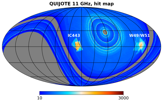
Figure 1: Map showing the number of hits per pixel (i.e., the number of $40\,\text{ms}$ samples in each $N_{\rm side}=512$ pixel) for the combined wide survey and raster scan data set (see Section 3.2 for details). The inclusion of raster scans determines a local increase in sensitivity towards the IC443 region and the area surrounding W49 and W51. The map is centred at Galactic coordinates $(l,b)=(180^{\circ},0^{\circ})$ to better display the source areas. This map is obtained using 11 GHz data in total intensity, but the hit maps for the other frequency bands are qualitatively similar.

2.2 W51

The W51 region is located on the Galactic plane east of W49, at central coordinates $(l_{\rm eff},b_{\rm eff})=(49.20^{\circ},-0.35^{\circ})$. It was also initially discovered in Westerhout (1958) radio survey, as another bright source in Aquila, and initially classified as an HII region. Subsequent radio observations identified the source as a molecular cloud (Penzias et al., 1971) and allowed to further separate the region into three main substructures (Kundu & Velusamy, 1967; Mufson & Liszt, 1979): W51A and W51B, responsible for the observed thermal emission, and a non-thermal component W51C (for a detailed review of W51 morphology see Ginsburg, 2017).

W51A and W51B are located at Galactic coordinates $(l,b)=(49.48^{\circ},-0.33^{\circ})$ and $(l_{\rm eff},b_{\rm eff})=(49.1^{\circ},-0.3^{\circ})$, respectively; these regions are embedded in a giant molecular cloud of $M>10^{6}\,\text{M}_{\odot}$ (Carpenter & Sanders, 1998), with W51A the main star-forming component. W51A is one of the most studied regions of massive star formation in our Galaxy; its rich morphology allows to distinguish two main components, named G49.5-0.4 and G49.4-0.3 (Wilson et al., 1970). These components are further resolved into several regions (Martin, 1972; Mehringer, 1994; Okumura et al., 2000), among which we can cite the protoclusters IRS1 and IRS2 (Ginsburg et al., 2016). Several hyper-compact HII regions have also been detected with radio data (Ginsburg et al., 2020; Rivera-Soto et al., 2020). This complex structure, combined with the local richness in gas and dust content, makes this region the ideal environment to study high-mass star formation (Saral et al., 2017; Ginsburg et al., 2017; Goddi et al., 2020). Despite all the observational endeavours, however, W51A stellar population is likely not completely catalogued (Binder & Povich, 2018); recent studies of W51A using IR observations can be found in Lim & De Buizer (2019) and Bik et al. (2019), who confirmed the complexity of the ongoing star formation processes. The region also shows a rich astrochemistry (Vastel et al., 2017; Watanabe et al., 2017), which has been the object of studies searching for prebiotic molecules in star-forming regions (Rivilla et al., 2016, 2017; Jacob et al., 2021). The parallax distance to this molecular cloud has been estimated from maser observations as $d=5.41^{+0.31}_{-0.28}\,\text{kpc}$ (Sato et al., 2010) and as $d=5.1^{+2.9}_{-1.4}\,\text{kpc}$ (Xu et al., 2009), depending on the considered subregion; these estimates place W51 in the Carina-Sagittarius arm.

W51B appears as a filamentary structure populated by UCHII regions; however, unlike W51A, most of the star formation in W51B seems to have already taken place, as suggested by the lower fraction of dense gas (Ginsburg et al., 2015).

W51C is an extended source of non-thermal radio emission located west of W51A and mostly south of W51B at $(l_{\rm eff},b_{\rm eff})=(49.2^{\circ},-0.7^{\circ})$, which has been identified as a SNR (Seward, 1990) with an estimated age of 30 kyr (Koo et al., 1995). This source has been extensively observed in radio wavelenghts (Zhang et al., 2017; Ranasinghe & Leahy, 2018), X-rays (Koo et al., 2005; Hanabata et al., 2013) and $\gamma$-rays (Abdo et al., 2009; Aleksić et al., 2012). The distance of this SNR was first placed at 4.1 kpc (Sato, 1973); later, Koo et al. (1995) estimated the distance to be $\sim 6\,\text{kpc}$, although with a high uncertainty given that this result is based on the association of the SNR with a molecular cloud which may extend over 1.5 kpc. Observations of the HI 21-cm line in absorption led to an estimated distance of 4.3 kpc (Tian & Leahy, 2013) which has been recently re-evaluated as 5.4 kpc (Ranasinghe & Leahy, 2018). The latter result is dictated by the observed interaction between W51C and W51B (Koo & Moon, 1997; Brogan et al., 2013), which constrains the SNR to be at the same distance as the other W51 HII regions.

Table 2: Summary of the information on the QUIJOTE-MFI observations centred on each source; the last column reports the mean fractional wide survey (WS) time contribution to the final maps, computed with respect to the total time obtained combining the selected raster data with the nominal mode data. See 3.1 for more details.

Source	Observation type	Observing dates	Covered area	Total observing time	Selected time fraction	WS time fraction
W49	193 drift scans (73 min)	June-August 2015	616 deg2	235.6 h	78%	20%
W51	170 drift scans (74 min)	October-December 2016	708 deg2	209.1 h	73%	20%
IC443	552 raster scans (29 min)	October 2014 – June 2015	474 deg2	269.1 h	66%	21%

Overall, W51 has a luminosity to mass ratio similar to W49 (Eden et al., 2018); it subtends a region with diameter $\sim 50^{\prime}$ on the sky (Bik et al., 2019). The search for AME in the region has been tackled by Demetroullas et al. (2015), where it is shown that a spinning dust component is not required for a proper modelling of W51 intensity spectrum. To our knowledge, no clear evidence of AME emission towards W51 has been reported in the literature.

2.3 IC443

IC443 (Index Catalogue 443) is a SNR located in the constellation of Gemini at Galactic coordinates $(l,b)=(189.06^{\circ},3.24^{\circ})$; it is therefore found close to the Galactic anticentre, with a lower emission from the neighbouring background compared to W49 and W51, which are much closer in projection to the Galactic bulge. This source has been extensively observed throughout the whole spectrum, including radio (Kundu & Velusamy, 1972; Green, 1986; Castelletti et al., 2011; Mitra et al., 2014; Planck Collaboration et al., 2016a; Egron et al., 2016, 2017), optical (Fesen, 1984; Ambrocio-Cruz et al., 2017), X-ray (Petre et al., 1988; Matsumura et al., 2017; Greco et al., 2018; Hirayama et al., 2019; Zhang et al., 2018) and $\gamma$-ray (Torres et al., 2003; Tavani et al., 2010) frequencies. IC443 angular size is $\sim 45^{\prime}$ (Green, 2014); the related supernova event occured in between 3 (Petre et al., 1988) and 30 kyr ago (Olbert et al., 2001), with more recent estimates favouring $\sim 20$ kyr (Lee et al., 2008). The distance to IC443 is still under debate; estimates range in between 0.7 and 1.5 kpc (Lozinskaya, 1981; Fesen, 1984), with the latter value being the most commonly used in the literature. A higher distance of 1.5-2 kpc has been proposed due to IC443 association with the HII region Sh2-249 (Gao et al., 2011, see also Fig. 4); a more recent estimate by Ambrocio-Cruz et al. (2017) locates IC443 at 1.9 kpc from the Sun.

At radio frequencies IC443 shows two roughly spherical sub-shells of synchrotron emission, with different centres and radii (Onić et al., 2017); the region appears brighter in its north-eastern limb in equatorial coordinates. These shells traditionally define the boundary of IC443; a fainter and larger shell has been detected, but it is not clear whether it is a different SNR, nor if it is actually interacting with IC443 (Lee et al., 2008). Radio thermal emission towards the region has also been observed, and ascribed to bremmstrahlung (Onić et al., 2012). X-ray observations, instead, reveal a centrally-filled profile, which makes IC443 a mixed-morphology or thermal-composite SNR (Rho & Petre, 1998; Rajwade et al., 2016). IC443 evolution and observed structure is the result of the interaction between the SNR and different phases of the surrounding interstellar medium (Lee et al., 2008; Ritchey et al., 2020; Koo et al., 2020; Ustamujic et al., 2021), with observational evidence of interaction with molecular gas in the southeast and northwest (Su et al., 2014; Yoshiike et al., 2017) and with an atomic cloud in the northeast (Kokusho et al., 2013). Observations in $\gamma$-rays towards IC443 are relevant for the study of Galactic cosmic rays; in particular, $\gamma$-ray emission deriving from the decay of pions (the “pion-decay bump”) has been detected by Ackermann et al. (2013). These pions are produced in collisions between accelerated cosmic-ray protons and interstellar material, so that the detection of the pion bump provides a direct evidence for the occurrence of proton acceleration in SNRs (Huang et al., 2020).

Finally, IC443 has already been a target in the search for AME. Onić et al. (2017) analised the radio and microwave spectrum of the region, reporting hints of AME detection and a bending of the synchrotron spectrum; however, they stressed that further data in the range 10 to 100 GHz are required to confirm these results. A similar conclusion was reached by Loru et al. (2019), who detected a clear bump in the range 20–70 GHz in IC443 intensity spectrum.

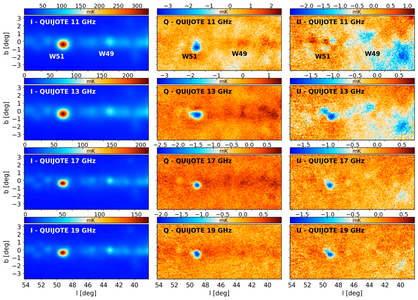
Figure 2: Intensity and polarisation destriped maps of the sky region including the sources W49 and W51, for the four QUIJOTE frequencies. All maps are shown here at their original resolution.

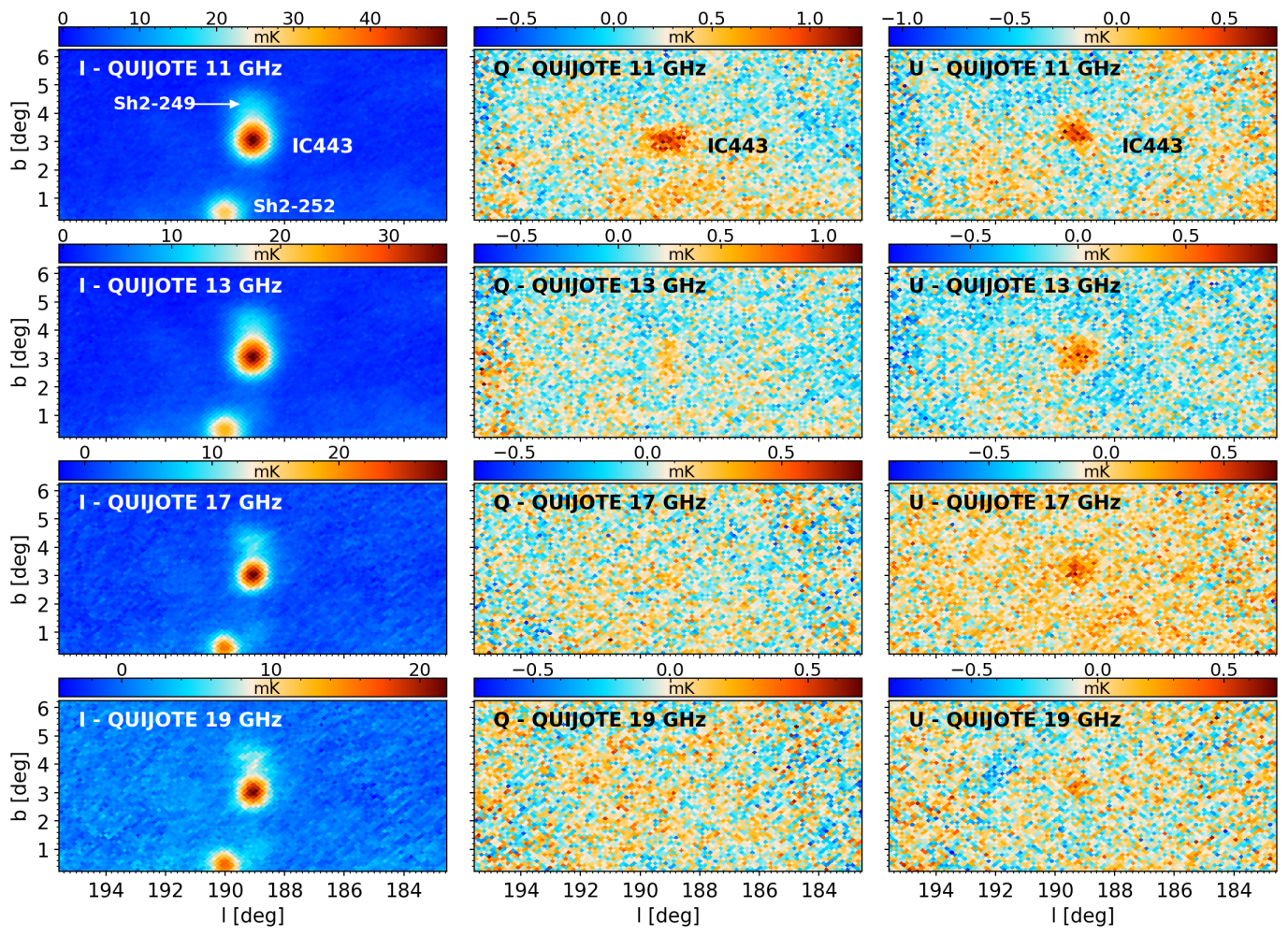
Figure 3: Same as in Fig. 2, but showing this time the IC443 region. The 11 GHz intensity map also marks the position of the two HII complexes surrounding the SNR.

3 QUIJOTE data

We present in this work data acquired with the QUIJOTE experiment (Génova-Santos et al., 2015a; Rubiño-Martín et al., 2017), a scientific collaboration aimed at characterising the polarisation of the CMB, and other Galactic and extra-Galactic physical processes, in the frequency range 10–40 GHz and at angular scales larger than 1 degree. QUIJOTE consists of two telescopes and three instruments, operating from the Teide Observatory (Tenerife, Spain), a site that provides optimal atmospheric conditions for CMB observations in the microwave range (Rubiño-Martín et al., 2012b).

The data used in this work were acquired with the QUIJOTE multi-frequency instrument (MFI, Hoyland et al., 2012), which consists of four conical corrugated feedhorns, each feeding a novel cryogenic on-axis polar modulator that can be rotated in steps of $22.5^{\circ}$. The output from each horn consists of eight channels carrying different linear combinations of the radiation Stokes parameters, which in turn are separated by the subsequent data analysis pipeline. Horns 1 and 3 both observe at frequency bands centred at 11 and 13 GHz, whereas horns 2 and 4 both observe at frequency bands centred at 17 and 19 GHz, all with a 2 GHz bandwidth. The full width at half-maximum (FWHM) is equal to 52 arcmin for the two low-frequency horns and to 38 arcmin for the two high-frequency horns. Overall, the MFI provides eight different maps of the sky in intensity and polarisation, and is primarily devoted to the characterisation of the Galactic emission. A full description of the MFI data reduction pipeline and map-making is provided in Génova-Santos et al. (2023).

3.1 Observations

The analysis presented in this paper is based on the combination of different QUIJOTE observations. We first consider data from the MFI wide survey, which covers more than $25,000\,\text{deg}^{2}$ including most of the northern sky, and as such encompasses the three regions targeted in this study. Observations were performed at fixed elevation by letting the telescope spin continuously in azimuth, and took place between May 2013 and June 2018 for a total observing time of $\sim 9200\,\text{h}$. The removal of bad data performed by the pipeline yields an effective total time of $\sim 8500\,\text{h}$ in intensity and in the range $\sim 4700\,\text{h}$ to $\sim 6800\,\text{h}$ in polarisation, depending on the chosen horn; the resulting data were used to produce the QUIJOTE wide survey legacy maps. An extensive description of the MFI wide survey and its associated data products can be found in Rubiño-Martín et al. (2023). On top of this large scale survey, we also consider a set of dedicated raster scan observations focussed on each region, which we describe in the following; we stress that the raster scan observations constitute the major source of data used in the current analysis. A summary of the related information is also reported in Table 2.

W49 was mapped in 193 dedicated observations performed between June and August 2015; these observations were drift scans in which the telescope elevation was maintained fixed and the pointing was switched back and forth in azimuth with an $\sim 18/\cos{(\text{EL})}$ deg amplitude for each scan; each observation took on average 73 min, and covered a final mean area of $408\,\text{deg}^{2}$ per horn on the sky. Notice that the MFI focal plane configuration determines a different pointing for each horn for the same observation, with separations up to $\sim 5^{\circ}$; this extends the sky area covered by W49 rasters to $616\,\text{deg}^{2}$. The total observing time is 235.6 h; after the inspection and removal of bad data, which is performed for each horn independently, the effective observing times for the four horns are 171.4, 194.1, 177.0 and 189.5 h, corresponding to a an average of $\sim 78\%$ of the total. After combining the good raster data with the nominal mode data, the latter account for 13.4%, 29.0%, 19.0% and 19.8% of the total observing time in each horn; on average, the wide survey fractional time contribution to the final maps in the W49 region is $\sim 20\%$.

W51 is located $\sim 6\,\text{deg}$ east of W49 on the Galactic plane, so it was also captured by the drift scans we just described. However, due to the different horn sky coverage, W51 was only partially mapped in several observations. For this reason it was decided to perform an independent set of observations centred on W51: they were conducted between October and December 2016, as a set of 170 fixed-elevation scans with a $\sim 20/\cos{(\text{EL})}$ deg azimuth amplitude, each lasting 74 min on average. The total observing time is 209.1 h, which after the good data selection amounts to 140.9, 152.7, 158.8 and 155.3 h for the four horns, corresponding to an average of $\sim 73\%$ of the total time. In this case, the nominal mode data contribute for 14.7%, 21.3%, 25.7% and 17.3% of the total observing time in each horn after combination with raster data; again, the mean wide survey time contribution to the final maps is $\sim 20\%$. Each horn covers on average $534\,\text{deg}^{2}$ on the sky, for a total $708\,\text{deg}^{2}$ mapped by the MFI with this set of observations. The overall sky area covered by the joint set of observations of W49 and W51 amounts to $891\,\text{deg}^{2}$, thus enabling an extended reconstruction of the Galactic plane region surrounding the two molecular complexes.

Finally, IC443 was targeted by 552 observations conducted between October 2014 and June 2015. In this case the observations consisted in raster scans with an amplitude of $\sim 12/\cos{(\text{EL})}$ deg in azimuth, with the telescope being stepped $\sim 0.1$ deg in elevation at the end of each scan, over a total $\sim 12$ deg range. Each observation lasted 29 min on average, for a total observing time of 269.2 h. The selection of good data yielded 174.3, 192.8, 187.6 and 159.5 h for the four horns, averaging at $\sim 66\%$ of the overall dedicated time. Out of the combination with nominal mode data, the latter account for 10.2%, 22.3%, 24.0% and 27.9% of each horn observing time, for an average time fraction of $\sim 21\%$. The mean area covered by each horn amounts to $360\,\text{deg}^{2}$, for a total $474\,\text{deg}^{2}$ mapped by the MFI in this region.

3.2 Maps

Time-ordered data from the raster scan observations are processed adopting the standard QUIJOTE pipeline described in Génova-Santos et al. (2023). Subsequently, these data are combined with data from the wide survey to produce the associated sky maps. The map-making is based on the PICASSO code (Guidi et al., 2021) with the same set of destriper parameters (noise priors and baseline length) adopted in Rubiño-Martín et al. (2023) when producing maps of the wide survey data alone. The resulting destriped map is provided using a HEALPix pixelisation (Górski et al., 2005) with $N_{\rm side}=512$, corresponding to a 6.9 arcmin pixel size; this resolution is enough given that the MFI beam FWHM values are larger than 0.5^∘. The code provides full sky maps, with increased sensitivities towards the relevant regions thanks to the inclusion of raster scan data; this is visible in the hit map shown in Fig. 1, where we can clearly distinguish two regions with higher integration time, one centred on the Galactic plane around W49 and W51, and one centred on IC443. In the following we will focus on sub-maps centred on these specific areas. We remind that the wide survey maps presented in Rubiño-Martín et al. (2023) are corrected for residual radio frequency interference contamination by subtracting the median value of pixels in rings of constant declination (FDEC correction, see Sec. 2.4.2 in the aforementioned reference). However, as in this analysis we will only perform aperture photometry measurements (Sec. 5), this correction is unnecessary and is not applied to our combined wide survey plus raster scan maps. A quantitative estimation of the impact of FDEC on aperture photometry measurements is presented in appendix B1 in Rubiño-Martín et al. (2023), and is well below the uncertainties associated with our measurements presented in Sec. 5.

Local maps for W49/W51 and IC443 are plotted in Fig. 2 and in Fig. 3 respectively, in the three Stokes parameters $I$, $Q$ and $U$, for the four MFI frequencies. Although in our subsequent analysis we will consider all maps smoothed to a common resolution of $1\,\text{deg}$, these plots show the maps in their original resolution. As two horns cover each frequency band, their individual maps are combined to yield the final map of the corresponding band. However, for the low frequency bands (11 and 13 GHz) the maps we employ are the ones obtained from horn 3 data alone; this is due to a fault in the polar modulator of horn 1, which has been fixed to the same position since September 2012, thus making data obtained with this horn not reliable. For the case of 17 and 19 GHz, instead, the maps we show are obtained from a linear combination of horn 2 and horn 4 maps, each weighted by a uniform weight computed from the white noise in the power spectrum of the associated wide survey map (for details see Rubiño-Martín et al., 2023).

Table 3: Results of the null test performed on QUIJOTE maps. For each frequency and Stokes parameter we compare the 1-degree beam rms obtained in the original map (Map) and in the null test map (NT). The last column reports the resulting MFI instantaneous sensitivity in polarisation.

Frequency	$\sigma_{I}$ [$\mu$K$\,\text{beam}^{-1}$]			$\sigma_{Q}$ [$\mu$K$\,\text{beam}^{-1}$]			$\sigma_{U}$ [$\mu$K$\,\text{beam}^{-1}$]			$\sigma_{Q,U}$ [mK$\,\text{s}^{1/2}$]
[GHz]	Map	NT		Map	NT		Map	NT		NT
W49/W51
11.0	617.4	53.8		25.8	22.5		21.9	21.3		1.4
13.0	489.8	34.6		18.9	16.2		15.9	15.1		1.2
17.0	300.7	57.5		14.1	13.1		13.8	13.2		1.4
19.0	252.9	71.7		15.9	12.8		15.3	14.6		1.4
IC443
11.0	71.1	59.8		21.2	19.6		21.1	20.0		1.1
13.0	52.2	44.7		20.1	18.4		18.4	19.0		1.0
17.0	80.9	62.4		16.0	15.3		19.2	15.8		1.2
19.0	100.1	79.3		18.8	17.6		19.2	17.1		1.4

In Fig. 2 we show the QUIJOTE maps for the Galactic plane region encompassing the sources W49 and W51. The Galactic plane is easily recognisable in the intensity maps, as a stripe of diffuse emission surrounding the compact objects; this diffuse emission is also visible in polarisation, with the expected imprint of positive $Q$ and nearly zero $U$. In intensity both W49 and W51 are clearly visible; at the western edge of the intensity maps it is possible to see the border of the source W47, which was studied in Génova-Santos et al. (2017). W51 appears particularly bright in these maps; it saturates the chosen colour scales in intensity, while in polarisation it shows a clear emission with both negative $Q$ and $U$, which makes it stand out from the diffuse Galactic plane polarisation signal. As commented in Section 2.2, W51 size is $\sim 50^{\prime}$, which means it is partially resolved with QUIJOTE beams; indeed, a mismatch is visible between the centres of the intensity and polarisation emissions, with $Q$ and $U$ peaks being slightly displaced towards the south-east. A possible explanation for this is that while the bulk of the intensity emission comes from the molecular cloud hosting W51A, the polarised emission is from the SNR W51C only. W49 appears fainter in intensity, and does not reveal a clear hint of polarised emission, although the diffuse Galactic plane polarisation shows an increment in positive $Q$ at the source position. Unlike W51, there is no particular internal structure visible for this source; its angular size of $\sim 30^{\prime}$ implies it is not resolved by QUIJOTE.

IC443 maps are shown in Fig. 3. As commented in Section 2.3, the source is located towards the Galactic anticentre and at a Galactic latitude of $\sim 3^{\circ}$, therefore the Galactic plane emission is not visible in these maps; its outskirts, however, still enter the maps as a background emission gradient that increases towards the south. In addition, two radio sources are visible in the vicinity of IC443: a bright source towards the southeast, which we can identify as the HII region Sh2-252 (also referred to as NGC2174, Bonatto & Bica, 2011) and a fainter feature just north of the SNR, which produces an apparent elongation of IC443 in that direction and can be ascribed to the HII region Sh2-249 (Dunham et al., 2010; Gao et al., 2011). The emission from these sources can affect the flux density estimates in this region; therefore, we apply to all IC443 maps an ad hoc mask built to block the contribution of the neighbouring objects. The details of the mask are visible in the right panel of Fig. 4. In the QUIJOTE intensity maps the source is clearly detected, although the background at 19 GHz is noisier compared to the maps obtained for W49 and W51; in polarisation the maps show a positive $U$ emission and hints of a positive $Q$ emission (with a more significant detection at 11 GHz) towards the source, which can be ascribed to synchrotron emission proceeding from the SNR.

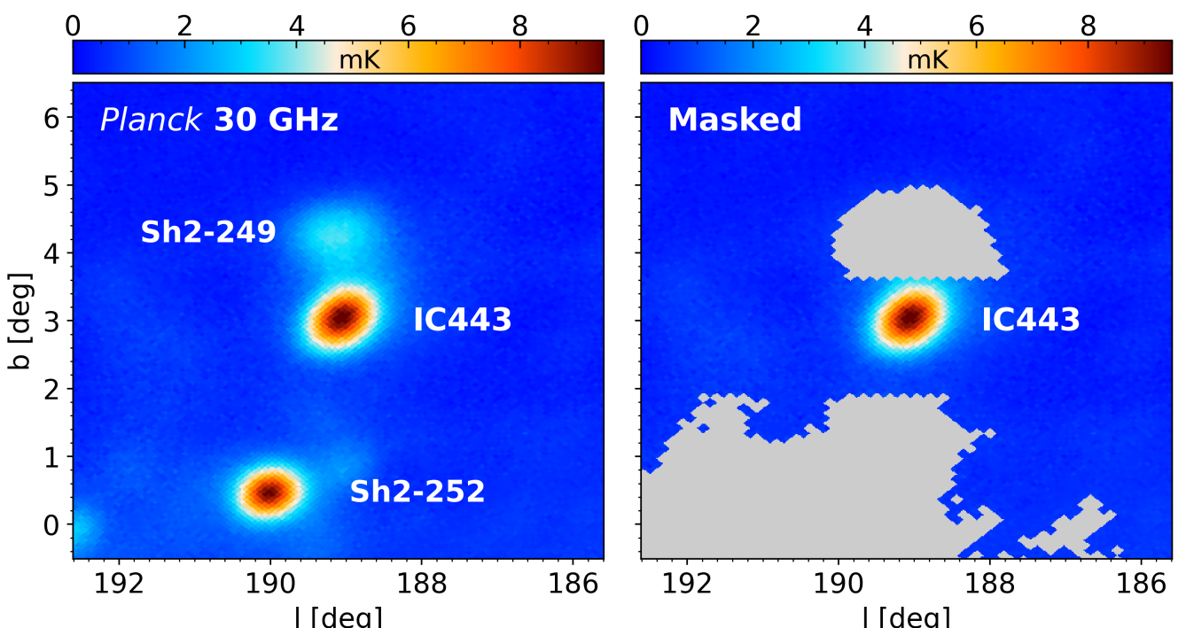
Figure 4: Left. The area surrounding IC443 shown on the Planck 30 GHz map (2015 data release). Right. The same area after applying a tailored mask which excises the contribution from the HII regions Sh2-249 and Sh2-252.

3.3 Null-test maps and noise levels

We use a null test map built from QUIJOTE data to evaluate the contribution of instrumental noise. For each observed region, we split the available data in two halves with the same number of observations, in such a way that each half has a sky coverage as similar as possible as the other; for the wide survey data we use the same halves as in Rubiño-Martín et al. (2023). In order to allow a proper reconstruction of the polarised signal from each half, care is taken to split observations in such a way that the distribution of observations in each polar modulator position is the same in both halves. For each half we then generate the corresponding maps adopting the same processing pipeline that was used for the full data set. We then obtain the null-test maps as:

$$M_{\rm NT}=\frac{1}{2}\left(M_{\rm H1}-M_{\rm H2}\right),$$ (1)

where $M_{\rm H1}$ and $M_{\rm H2}$ represent the first and second half maps. By construction, the resulting map $M_{\rm NT}$ should be free from the sky signal, which cancels out in the subtraction, and be representative of the instrumental contribution only. We compute the instrumental noise component as the rms of the pixel values found in a 1-degree radius aperture on each null map. The resulting quantity represents the rms of individual pixels; to be consistent with other QUIJOTE works, we convert it into the rms of a Gaussian beam with FWHM=$1^{\circ}$, by dividing the original rms by the square root of the number of pixels entering the beam solid angle. We place our aperture far from the sources, centred at $(l,b)=(46^{\circ},-2^{\circ})$ for the W49/W51 map, and at $(l,b)=(186^{\circ},2.5^{\circ})$ for the IC443 map; this choice allows us to compare this rms with the same quantity evaluated on the full data set maps. The two values of rms are directly comparable thanks to the factor $1/2$ in equation (1), which cancels the $\sqrt{2}$ factor coming from the linear combination of the two half-maps, and the additional $\sqrt{2}$ factor coming from the splitting of the available statistics, that increases the rms of each half-map. The comparison for the Stokes parameters $I$, $Q$ and $U$ is reported in Table 3 for both the W49/W51 and the IC443 maps.

We see that in polarisation the real maps and the null-test maps have similar rms values, which means that the main contribution to the polarisation maps used in this study is noise. For intensity, instead, the rms is considerably higher when evaluated in the full data maps than in the null-test maps. This is indicative of an important contribution from the sky emission in the estimation of the noise. The effect is stronger for the W49/W51 map due to the proximity of the regions to the Galactic plane, which introduces gradients in the background signal. The polarisation rms values quoted in Table 3 are about a factor 2 lower than the ones obtained from the wide survey maps only (Rubiño-Martín et al., 2023); this shows the improvement in the map quality achieved by including the dedicated raster scan observations towards our sources. In fact, the sensitivity in polarisation averages around $\sim 15\,\mu\text{K}/\text{beam}$, which is the deepest level reached by published QUIJOTE data so far.

The last column in Table 3 reports the instantaneous sensitivity of the maps in polarisation, computed by multiplying the quoted $Q$ and $U$ rms values per beam by the square root of the mean observing time per 1-degree beam; the results for $Q$ and $U$ are then averaged (in quadrature) to yield the values of $\sigma_{Q,U}$ reported in the table. In general, these estimates range from 1.0 to $1.4\,\text{mK}\,\text{s}^{1/2}$; this is expected, since the nominal instrument sensitivity in polarisation is $\sim 1\,\text{mK}\,\text{s}^{1/2}$. Our findings are consistent with previously reported values for the instantaneous sensitivity (Génova-Santos et al., 2015b, 2017). This test confirms the good quality of the polarisation maps, and that the instrumental noise contribution to the maps is controlled and within the expected limits.

Table 4: Summary of the ancillary data detailed in Section 4, which are used in combination with QUIJOTE data to broaden the considered frequency range. For each map we report the frequency, the reference telescope(s) or satellite, which Stokes parameters are available, the original map resolution and units, the applied calibration uncertainty and the reference in the literature.

Frequency	Facility	Stokes	Original resolution	Original	Calibration	Reference
$[\text{GHz}]$			[arcmin]	units	uncertainty [%]
0.408	Jodrell Bank MkI, MkIA-76 m,	$I$	51	K	10	Haslam et al. (1982); Platania et al. (2003)
	Bonn-100 m, Parkes-64 m
0.820	Dwingeloo-25 m	$I$	72	K	10	Berkhuijsen (1972)
1.410	DRAO-25.6 m	$Q,U$	36	mK	10	Wolleben et al. (2006)
1.420	Stockert-25 m, Villa-Elisa-30 m	$I$	36	K	10	Reich & Reich (1986); Platania et al. (2003)
2.326	HartRAO-26 m	$I$	20	K	10	Jonas et al. (1998); Platania et al. (2003)
4.800	Urumqi-25 m	$I,Q,U$	9.5	mK	10	Gao et al. (2010); Sun et al. (2011)
22.8	WMAP 9-yr	$I,Q,U$	50.7	mK	3	Bennett et al. (2013)
28.4	Planck-LFI	$I,Q,U$	32.29	K	3	Planck Collaboration et al. (2016b); Planck Collaboration et al. (2020e)
33.0	WMAP 9-yr	$I,Q,U$	38.8	mK	3	Bennett et al. (2013)
40.6	WMAP 9-yr	$I,Q,U$	30.6	mK	3	Bennett et al. (2013)
44.1	Planck-LFI	$I,Q,U$	27.00	K	3	Planck Collaboration et al. (2016b); Planck Collaboration et al. (2020a)
60.8	WMAP 9-yr	$I,Q,U$	20.9	mK	3	Bennett et al. (2013)
70.4	Planck-LFI	$I,Q,U$	13.21	K	3	Planck Collaboration et al. (2016b); Planck Collaboration et al. (2020a)
93.5	WMAP 9-yr	$I,Q,U$	14.8	mK	3	Bennett et al. (2013)
100	Planck-HFI	$I,Q,U$	9.68	K	3	Planck Collaboration et al. (2016b); Planck Collaboration et al. (2020a)
143	Planck-HFI	$I,Q,U$	7.30	K	3	Planck Collaboration et al. (2016b); Planck Collaboration et al. (2020a)
217	Planck-HFI	$I,Q,U$	5.02	K	3	Planck Collaboration et al. (2016b); Planck Collaboration et al. (2020a)
353	Planck-HFI	$I,Q,U$	4.94	K	3	Planck Collaboration et al. (2016b); Planck Collaboration et al. (2020a)
545	Planck-HFI	$I$	4.83	MJy/sr	6.1	Planck Collaboration et al. (2016b)
857	Planck-HFI	$I$	4.64	MJy/sr	6.4	Planck Collaboration et al. (2016b)
1249	COBE-DIRBE	$I$	37.1	MJy/sr	11.9	Hauser et al. (1998)
2141	COBE-DIRBE	$I$	38.0	MJy/sr	11.9	Hauser et al. (1998)
2998	COBE-DIRBE	$I$	38.6	MJy/sr	11.9	Hauser et al. (1998)

4 Ancillary data

In order to better characterise the emission from the Galactic regions considered in this study, we also employ ancillary data that extend the information provided by QUIJOTE observations to both lower and higher frequencies. We use all maps in a common HEALPix pixelisation of $N_{\rm side}=512$, and at a common angular resolution of $1\,\text{deg}$. With the exception of WMAP maps, which are already available at this angular resolution at the LAMBDA website, in all the other cases the smoothed maps are obtained by deconvolving the original beam (the nominal survey FWHM was used in each case and a Gaussian beam shape was assumed) and convolving with a 1 deg FWHM Gaussian beam. QUIJOTE maps are also degraded to this coarser resolution for the photometric analysis. The relevant properties of all the ancillary maps used in this study are summarised in Table 4.

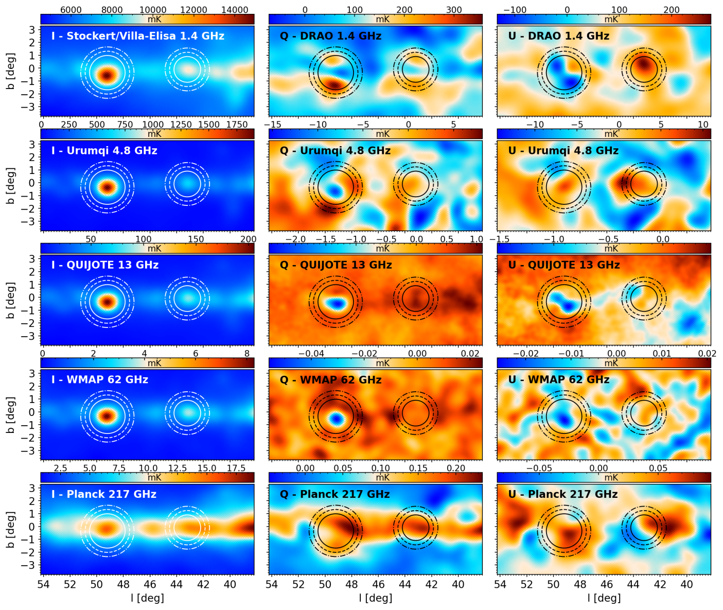
Figure 5: Sample intensity and polarisation maps of the sky region including the sources W49 and W51, degraded to a 1 deg resolution, across the frequency range employed for the SED study. The apertures and background annuli used for the aperture photometry analysis are overplotted to each panel.

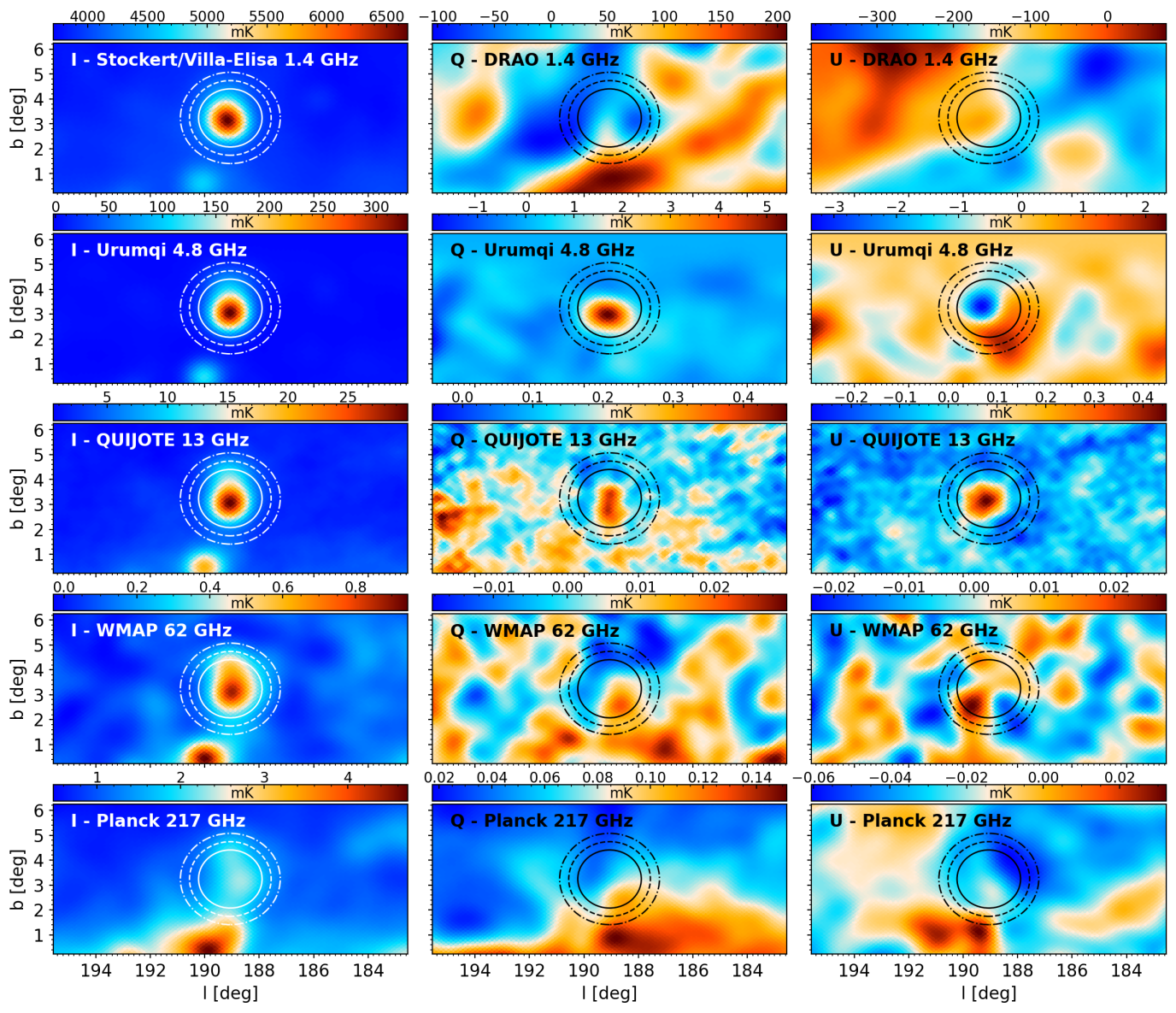
Figure 6: Same as in Fig. 5, but showing this time the IC443 region. The mask is not included to better show the evolution of the background with frequency.

4.1 Lower frequency ancillary data

In the radio and microwave domains we consider the map at 408 MHz from Haslam et al. (1982) survey, which covers the whole sky with observations from different facilities (Jodrell Bank MkI and MkIA-76 m, Bonn-100 m and Parkes-64 m telescopes), the Berkhuijsen (1972) map at 820 MHz, obtained from a survey with the Dwingeloo-25 m telescope, the Reich & Reich (1986) survey at 1420 MHz conducted with the Stockert-25 m and the Villa-Elisa-30 m telescopes, and the Jonas et al. (1998) survey at 2326 MHz obtained with the HartRAO-26 m telescope.

We actually use the 408, 1420 and 2326 MHz maps provided by Platania et al. (2003), which are corrected for the artifacts produced by observational strategy and instrumental gain drifts; the 820 MHz map is instead generated by projecting into HEALPix pixelisation the corresponding observational data retrieved from the MPIfR’s Survey Sampler. These radio maps only provide intensity data and are calibrated referring to the full-beam solid angle; as explained in Reich & Reich (1988), the sidelobe contribution would lead to an underestimation of the flux density for sources which are small compared to the main beam. This effect is particularly important for the Reich & Reich (1986) survey, and in the aforementioned reference it is argued that a correction factor of 1.55 can be used to account for the flux density loss. Since the FWHM for the Stockert telescope is $\sim 35^{\prime}$, this factor can be applied for W49, but not for W51 and IC443, whose angular sizes are larger than the survey beam; in these cases, we employed a more conservative value of 1.25. These multiplicative factors are employed to correct the flux densities extracted from the 1420 MHz map in the aperture photometry analysis described in Section 5. Although a similar issue affects the 2326 MHz map, we do not apply any explicit correction as the HartRAO beam is considerably smaller (20’) than the size of our sources. It is worth mentioning that the HartRAO map, which we use for the total intensity signal, actually carries the combination $I+Q$, and can consequently yield biased estimates of $I$ flux densities towards polarised regions. However, as it is clear from the photometric analysis results in section 5, the polarised flux density is typically $<2\%$ of the flux density in total intensity, and the conservative 10% calibration uncertainty adopted for the HartRAO measurement (see again Section 5) is enough to account for this bias.

In polarisation we consider the survey carried out by the Dominion Radio Astronomy Observatory (DRAO, Wolleben et al., 2006), which provides Stokes $Q$ and $U$ maps for the northern sky at 1.41 GHz. We stress that the DRAO maps are delivered7 following the IAU convention for the definition of the Stokes parameters; hence, we adapt it to the convention chosen in this work by flipping the sign of the $U$ map. Finally, we employ the intensity and polarisation maps from the Sino-German $6\,\text{cm}$ survey of the Galactic plane (Gao et al., 2010; Sun et al., 2011), conducted with the Urumqi-25 m telescope at 4.8 GHz.

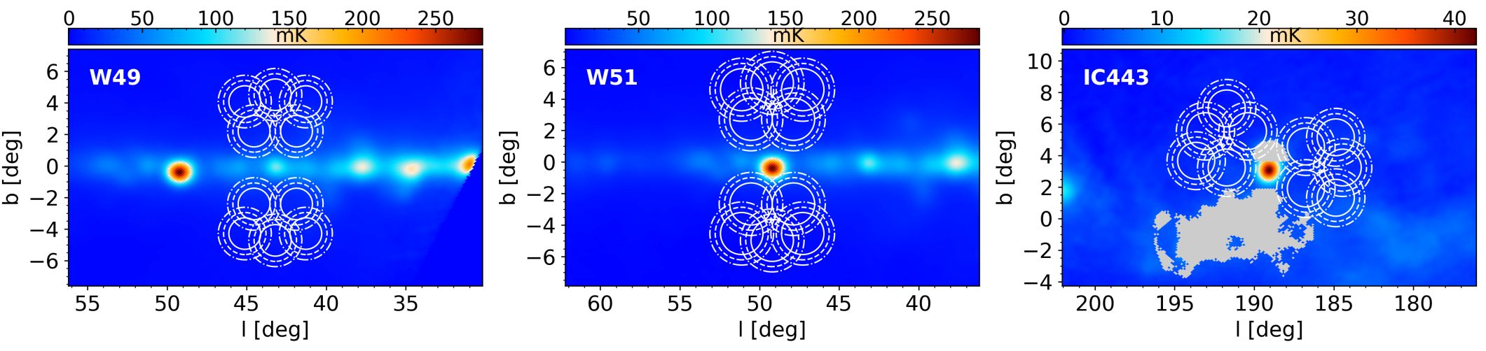
Figure 7: Random apertures employed to estimate the uncertainties on the source flux densities, overplotted for all three regions onto QUIJOTE 11 GHz maps smoothed to a 1 deg resolution. The IC443 tailored mask is also shown in the third panel. The size of the central apertures and the background annuli are the same as the ones used for measuring the source flux density.

4.2 Higher frequency ancillary data

In the microwave and far-infrared (FIR) range we employ data from the CMB satellite missions WMAP, Planck and COBE. We consider the five WMAP bands at 23, 33, 41, 61, and 94 GHz, using the corresponding maps in the Stokes parameters $I$, $Q$ and $U$ from the 9-year WMAP data release (Bennett et al., 2013), available at the LAMBDA data base.

As per the Planck data, we use the maps from the second data release (Planck Collaboration et al., 2016b), which are publicly available at the Planck Legacy Archive (PLA) webpage. The website provides the nine individual frequency survey maps in intensity, at 30, 44 and 70 GHz from the Low Frequency Instrument (LFI), and at 100, 143, 217, 353, 545 and 857 GHz from the High Frequency Instrument (HFI). The 100, 217 and 353 maps are contaminated by the CO rotational transition lines (1–0), (2–1) and (3–2) respectively, so these maps were first corrected using the Planck-released Type 1 CO maps (Planck Collaboration et al., 2014b), also available in the PLA webpage. In polarisation, instead, we use the available maps up to 353 GHz from the third data release (Planck Collaboration et al., 2020a), whose main improvement with respect to the second data release is precisely in the polarisation data. Since after a visual inspection of the maps we detected artifacts affecting the 30 GHz $U$ map towards W51, just for this frequency we adopt instead the polarisation maps obtained from the NPIPE pipeline (Planck Collaboration et al., 2020e).

Finally, we use the Zodi-Subtracted Mission Average maps from the DIRBE instrument on the COBE mission (Hauser et al., 1998) at 1249, 2141 and 2998 GHz; these maps are available in HEALPix format at the CADE data base. Maps for these frequencies are in total intensity only.

5 SED of sources

The characterisation of the emission from our sources is primarily achieved by analysing their spectral energy distribution (SED), i.e., the frequency dependence of the observed flux densities in intensity and polarisation. Flux densities are measured with the aperture photometry technique, following the implementation described in Génova-Santos et al. (2015b) and also adopted by Génova-Santos et al. (2017) and Poidevin et al. (2019) for the study of other compact sources. Apart from the previous QUIJOTE studies, aperture photometry has already been exploited for SED reconstruction in previous works (López-Caraballo et al., 2011; Dickinson et al., 2011; Génova-Santos et al., 2011; Rubiño-Martín et al., 2012a; Demetroullas et al., 2015; Planck Collaboration et al., 2016a). The technique consists in estimating the mean map temperature inside a suitable aperture centred on the source, and in removing a background level estimated as the median signal within a surrounding annulus; the result is then converted into flux density using the analytical conversion factor between temperature units and Jy, and the angular size subtended by the aperture. The sizes of the aperture and annulus depend on the considered source. We adopt the values reported in Table 1 which suit the different angular extents of the three regions; the table also reports the reference source position onto which all circles are centred. This choice is adopted for all the QUIJOTE and ancillary maps smoothed to a 1 deg resolution, and for measuring both the intensity and polarisation SEDs. The corresponding circles are overplotted to the intensity and polarisation maps shown in Figs 5 and 6. Notice that although in other works the background is estimated as the mean value of map pixels in the annulus, in our case the regions are close to the Galactic plane, implying that strong signal variation on scales comparable to our apertures may bias the estimation of the background level. The choice of the median of the annulus pixels is then made to minimize this effect, as discussed in Rubiño-Martín et al. (2012a).

Table 5: Summary table for the intensity and (when available) polarised flux densities obtained for W49 at different frequencies. Values for the Stokes parameters $I$, $Q$ and $U$ are extracted from the QUIJOTE and ancillary maps degraded at a 1 degree resolution, while the polarised intensity $P$, the polarised fraction $\Pi$ and the polarisation angle $\gamma$ are computed as detailed in Section 5. The last column reports the colour correction coefficients for intensity and polarisation, computed following the methodology described in Section 6.1; when polarisation data are not available we quote the colour correction in total intensity only.

W49
Survey	Freq.	$I$	$Q$	$U$	$P$	$\Pi$	$\gamma$	CC
	[GHz]	[Jy]	[Jy]	[Jy]	[Jy]	%	[deg]	$(I,P)$
Haslam	0.4	208$\pm$35	-	-	-	-	-	-
Berkhuijsen	0.8	167$\pm$23	-	-	-	-	-	-
Reich	1.4	134$\pm$16	-	-	-	-	-	-
DRAO	1.4	-	0.7$\pm$2.1	4.5$\pm$1.3	4.2$\pm$1.7	3.2${}^{+1.3}_{-1.4}$	-40.4$\pm$12.9	-
Jonas	2.3	105$\pm$13	-	-	-	-	-	-
Urumqi	4.8	150$\pm$16	2.6$\pm$7.8	3.6$\pm$7.8	$\lesssim$17.0	$\lesssim$11.2	-26.9$\pm$50.6	-
QUIJOTE	11.1	143$\pm$8	1.9$\pm$0.6	0.6$\pm$0.5	1.9$\pm$0.6	1.3${}^{+0.4}_{-0.5}$	-8.4$\pm$7.7	0.986, 0.974
QUIJOTE	12.9	148$\pm$8	1.3$\pm$0.6	0.2$\pm$0.3	1.2$\pm$0.4	0.8$\pm$0.3	-4.5$\pm$6.1	1.001, 0.998
QUIJOTE	16.8	158$\pm$9	1.2$\pm$0.3	0.2$\pm$0.2	1.2$\pm$0.3	0.7$\pm$0.2	-3.8$\pm$5.4	1.007, 1.019
QUIJOTE	18.8	160$\pm$9	1.2$\pm$0.3	0.2$\pm$0.2	1.2$\pm$0.3	0.8$\pm$0.2	-4.7$\pm$5.3	1.008, 1.012
WMAP	22.8	161$\pm$6	1.0$\pm$0.3	0.3$\pm$0.2	1.1$\pm$0.2	0.7$\pm$0.1	-7.8$\pm$4.8	0.973, 0.960
Planck-LFI	28.4	149$\pm$6	1.0$\pm$0.2	0.1$\pm$0.2	1.0$\pm$0.2	0.7$\pm$0.1	-2.9$\pm$4.1	1.006, 1.002
WMAP	33.0	144$\pm$5	0.8$\pm$0.3	0.1$\pm$0.2	0.8$\pm$0.3	0.5$\pm$0.2	-1.8$\pm$8.2	0.982, 0.978
WMAP	40.6	134$\pm$4	0.5$\pm$0.4	0.3$\pm$0.3	0.4${}^{+0.2}_{-0.4}$	$\lesssim$0.9	-16.7$\pm$16.1	0.994, 0.992
Planck-LFI	44.1	132$\pm$5	0.4$\pm$0.2	0.1$\pm$0.2	0.3$\pm$0.2	0.2${}^{+0.1}_{-0.2}$	-7.3$\pm$15.2	0.992, 0.991
WMAP	60.8	130$\pm$5	0.0$\pm$0.4	0.4$\pm$0.6	$\lesssim$1.2	$\lesssim$0.9	-42.4$\pm$33.8	0.977, 0.985
Planck-LFI	70.4	137$\pm$6	1.0$\pm$0.3	0.5$\pm$0.3	1.1$\pm$0.3	0.7${}^{+0.3}_{-0.2}$	-14.8$\pm$8.3	0.984, 0.985
WMAP	93.5	189$\pm$9	1.5$\pm$2.0	0.0$\pm$1.6	$\lesssim$4.3	$\lesssim$2.3	-0.7$\pm$31.3	0.993, 1.000
Planck-HFI	100.0	220$\pm$11	3.4$\pm$0.5	-0.1$\pm$0.3	3.4$\pm$0.4	1.5$\pm$0.2	1.1$\pm$2.4	0.965, 0.945
Planck-HFI	143.0	493$\pm$24	9.6$\pm$1.5	-0.2$\pm$0.9	9.6$\pm$1.2	1.9$\pm$0.3	0.6$\pm$2.7	0.984, 0.979
Planck-HFI	217.0	2021$\pm$109	43.2$\pm$6.5	5.7$\pm$4.2	43.2$\pm$5.2	2.1$\pm$0.3	-3.7$\pm$2.8	0.898, 0.896
Planck-HFI	353.0	9666$\pm$573	190.2$\pm$31.7	43.9$\pm$18.6	193.7${}^{+24.2}_{-24.3}$	2.0$\pm$0.3	-6.5$\pm$2.9	0.896, 0.900
Planck-HFI	545.0	(3.58$\pm$0.28) $\times 10^{4}$	-	-	-	-	-	0.887
Planck-HFI	857.0	(1.18$\pm$0.09) $\times 10^{5}$	-	-	-	-	-	0.961
DIRBE	1249.1	(2.66$\pm$0.32) $\times 10^{5}$	-	-	-	-	-	0.996
DIRBE	2141.4	(4.14$\pm$0.50) $\times 10^{5}$	-	-	-	-	-	1.075
DIRBE	2997.9	(2.13$\pm$0.26) $\times 10^{5}$	-	-	-	-	-	1.086

Table 6: Same as in Table 5, but for the W51 region.

W51
Survey	Freq.	$I$	$Q$	$U$	$P$	$\Pi$	$\gamma$	CC
	[GHz]	[Jy]	[Jy]	[Jy]	[Jy]	%	[deg]	$(I,P)$
Haslam	0.4	684$\pm$83	-	-	-	-	-	-
Berkhuijsen	0.8	653$\pm$71	-	-	-	-	-	-
Reich	1.4	411$\pm$43	-	-	-	-	-	-
DRAO	1.4	-	4.3$\pm$2.1	-6.3$\pm$1.9	7.4${}^{+2.0}_{-2.1}$	1.8${}^{+0.6}_{-0.5}$	27.8$\pm$7.7	-
Jonas	2.3	591$\pm$61	-	-	-	-	-	-
Urumqi	4.8	657$\pm$66	-3.0$\pm$8.4	2.7$\pm$8.4	$\lesssim$17.8	$\lesssim$2.7	-68.9$\pm$58.8	-
QUIJOTE	11.1	508$\pm$25	-4.4$\pm$0.8	-0.7$\pm$0.7	4.4$\pm$0.7	0.8${}^{+0.2}_{-0.1}$	85.3$\pm$4.4	0.982, 0.975
QUIJOTE	12.9	499$\pm$25	-5.6$\pm$0.6	-4.2$\pm$0.8	6.9$\pm$0.7	1.4$\pm$0.2	71.5$\pm$2.9	1.001, 0.998
QUIJOTE	16.8	502$\pm$25	-2.6$\pm$0.4	-3.4$\pm$0.5	4.3$\pm$0.4	0.8$\pm$0.1	64.0$\pm$2.8	1.008, 1.018
QUIJOTE	18.8	504$\pm$25	-3.2$\pm$0.5	-4.0$\pm$0.4	5.1$\pm$0.5	1.0$\pm$0.1	64.3$\pm$2.8	1.008, 1.011
WMAP	22.8	498$\pm$15	-3.2$\pm$0.2	-2.4$\pm$0.4	4.0$\pm$0.3	0.8$\pm$0.1	71.3$\pm$2.4	0.971, 0.963
Planck-LFI	28.4	470$\pm$14	-3.4$\pm$0.3	-1.8$\pm$0.3	3.8$\pm$0.3	0.8$\pm$0.1	76.4$\pm$2.5	1.006, 1.004
WMAP	33.0	466$\pm$14	-3.1$\pm$0.4	-1.6$\pm$0.4	3.5$\pm$0.4	0.7$\pm$0.1	76.2$\pm$3.2	0.982, 0.979
WMAP	40.6	435$\pm$13	-2.9$\pm$0.5	-1.4$\pm$0.4	3.2$\pm$0.5	0.7$\pm$0.1	77.4$\pm$3.8	0.995, 0.993
Planck-LFI	44.1	426$\pm$13	-2.9$\pm$0.2	-1.6$\pm$0.3	3.3$\pm$0.3	0.8$\pm$0.1	75.5$\pm$2.6	0.993, 0.991
WMAP	60.8	405$\pm$14	-2.1$\pm$0.9	-1.4$\pm$0.5	2.4$\pm$0.7	0.6$\pm$0.2	72.5$\pm$7.6	0.976, 0.972
Planck-LFI	70.4	406$\pm$14	-1.4$\pm$0.6	-1.2$\pm$0.5	1.7$\pm$0.5	0.4$\pm$0.1	70.2$\pm$8.1	0.985, 0.982
WMAP	93.5	481$\pm$23	-1.3$\pm$3.0	-1.1$\pm$1.9	$\lesssim$5.4	$\lesssim$1.1	69.7$\pm$41.1	0.988, 0.985
Planck-HFI	100.0	529$\pm$21	0.4$\pm$0.7	-1.9$\pm$0.4	1.8$\pm$0.6	0.3$\pm$0.1	39.0$\pm$10.8	0.976, 0.970
Planck-HFI	143.0	957$\pm$43	7.3$\pm$2.2	2.5$\pm$1.3	7.5$\pm$1.7	0.8$\pm$0.2	-9.5$\pm$5.4	0.986, 0.970
Planck-HFI	217.0	3545$\pm$197	39.3$\pm$9.2	15.1$\pm$4.7	41.6$\pm$6.6	1.2$\pm$0.2	-10.5$\pm$3.7	0.900, 0.870
Planck-HFI	353.0	(1.63$\pm$0.10) $\times 10^{4}$	159.5$\pm$43.1	93.0$\pm$19.9	182.3$\pm$29.3	1.1$\pm$0.2	-15.1$\pm$4.3	0.898, 0.870
Planck-HFI	545.0	(6.08$\pm$0.48) $\times 10^{4}$	-	-	-	-	-	0.887
Planck-HFI	857.0	(2.06$\pm$0.16) $\times 10^{5}$	-	-	-	-	-	0.958
DIRBE	1249.1	(4.82$\pm$0.59) $\times 10^{5}$	-	-	-	-	-	0.982
DIRBE	2141.4	(8.66$\pm$1.06) $\times 10^{5}$	-	-	-	-	-	1.081
DIRBE	2997.9	(5.60$\pm$0.68) $\times 10^{5}$	-	-	-	-	-	1.072

Table 7: Same as in Table 5, but for the IC443 region.

IC443
Survey	Freq.	$I$	$Q$	$U$	$P$	$\Pi$	$\gamma$	CC
	[GHz]	[Jy]	[Jy]	[Jy]	[Jy]	%	[deg]	$(I,P)$
Haslam	0.4	130$\pm$14	-	-	-	-	-	-
Berkhuijsen	0.8	132$\pm$13	-	-	-	-	-	-
Reich	1.4	81$\pm$8	-	-	-	-	-	-
DRAO	1.4	-	0.2$\pm$3.3	3.6$\pm$3.5	$\lesssim$8.9	$\lesssim$11.0	-43.4$\pm$26.4	-
Urumqi	4.8	88$\pm$8	1.6$\pm$1.0	-0.2$\pm$1.0	0.9${}^{+0.8}_{-0.9}$	$\lesssim$4.0	3.1$\pm$18.2	-
QUIJOTE	11.1	57$\pm$3	1.0$\pm$0.2	0.6$\pm$0.1	1.1$\pm$0.1	1.9$\pm$0.3	-15.8$\pm$3.5	0.977, 0.977
QUIJOTE	12.9	54$\pm$3	0.4$\pm$0.1	1.1$\pm$0.1	1.2$\pm$0.1	2.1$\pm$0.3	-36.2$\pm$3.6	1.000, 0.999
QUIJOTE	16.8	52$\pm$3	0.3$\pm$0.2	0.6$\pm$0.1	0.7$\pm$0.2	1.3${}^{+0.3}_{-0.4}$	-31.2$\pm$7.8	1.008, 1.017
QUIJOTE	18.8	51$\pm$3	0.1$\pm$0.3	0.4$\pm$0.4	$\lesssim$0.9	$\lesssim$1.8	-40.4$\pm$25.6	1.008, 1.011
WMAP	22.8	47$\pm$2	0.4$\pm$0.2	0.7$\pm$0.1	0.8$\pm$0.1	1.7$\pm$0.3	-29.6$\pm$4.9	0.966, 0.965
Planck-LFI	28.4	42$\pm$2	0.8$\pm$0.1	0.4$\pm$0.1	0.9$\pm$0.1	2.1$\pm$0.3	-13.8$\pm$3.5	1.005, 1.005
WMAP	33.0	40$\pm$2	0.4$\pm$0.3	0.6$\pm$0.2	0.7$\pm$0.2	1.7$\pm$0.6	-26.0$\pm$10.3	0.980, 0.981
WMAP	40.6	37$\pm$2	0.3$\pm$0.3	0.5$\pm$0.5	0.4${}^{+0.2}_{-0.4}$	$\lesssim$3.5	-31.8$\pm$15.1	0.994, 0.994
Planck-LFI	44.1	35$\pm$2	0.5$\pm$0.3	0.6$\pm$0.3	0.6${}^{+0.3}_{-0.4}$	1.8${}^{+0.9}_{-1.0}$	-24.5$\pm$12.5	0.992, 0.992
WMAP	60.8	33$\pm$5	0.5$\pm$1.4	0.8$\pm$1.3	$\lesssim$3.0	$\lesssim$9.3	-29.1$\pm$40.9	0.975, 0.973
Planck-LFI	70.4	33$\pm$5	-0.1$\pm$0.4	1.0$\pm$0.3	1.0$\pm$0.4	2.9${}^{+1.2}_{-1.4}$	-47.6$\pm$11.4	0.984, 0.984
WMAP	93.5	43$\pm$11	0.6$\pm$2.2	-0.4$\pm$2.7	$\lesssim$5.0	$\lesssim$11.6	15.3$\pm$102.5	0.989, 0.983
Planck-HFI	100.0	48$\pm$11	0.3$\pm$0.4	0.5$\pm$0.3	0.3$\pm$0.3	$\lesssim$2.8	-28.9$\pm$20.6	0.975, 0.988
Planck-HFI	143.0	80$\pm$23	0.5$\pm$0.6	1.0$\pm$0.7	0.9${}^{+0.5}_{-0.7}$	$\lesssim$3.4	-32.0$\pm$15.4	0.991, 0.987
Planck-HFI	217.0	282$\pm$84	3.7$\pm$3.4	2.9$\pm$2.6	2.8${}^{+2.3}_{-2.8}$	$\lesssim$4.2	-19.3$\pm$17.8	0.910, 0.893
Planck-HFI	353.0	1205$\pm$353	15.8$\pm$14.6	11.7$\pm$10.0	12.6${}^{+8.9}_{-12.6}$	$\lesssim$4.1	-18.2$\pm$17.2	0.907, 0.884
Planck-HFI	545.0	3934$\pm$1142	-	-	-	-	-	0.900
Planck-HFI	857.0	(1.09$\pm$0.31) $\times 10^{4}$	-	-	-	-	-	0.970
DIRBE	1249.1	(2.00$\pm$0.31) $\times 10^{4}$	-	-	-	-	-	1.013
DIRBE	2141.4	(2.54$\pm$0.40) $\times 10^{4}$	-	-	-	-	-	1.060
DIRBE	2997.9	(1.21$\pm$0.20) $\times 10^{4}$	-	-	-	-	-	1.088

The uncertainties on the measured flux densities can be computed as explained in Génova-Santos et al. (2015b), by using the rms of the pixels located in the background annulus (which is not biased by the source emission) and considering the contribution from the number of independent pixels in the aperture and in the annulus. We found that this method, although providing reasonable error estimates in total intensity, tends to underestimate the uncertainties in the $Q$ and $U$ flux densities. We then choose to compute the flux density errors, both in intensity and in polarisation, as the rms of the flux densities computed in 10 apertures randomly located around the source, in such a way as to avoid the diffuse emission from the Galactic plane region and other intervening compact sources. The chosen apertures are shown in Fig. 7 for all three regions; the radii for the central aperture and the background annulus are the same as the ones employed for computing the source flux densities. These error estimates capture the typical fluctuations of the background at the aperture scale, and represent therefore a more reasonable estimate for the flux density uncertainties.

We also include a calibration error a posteriori, which is taken as a fixed fraction of the measured flux density and added in quadrature to the rms of the random apertures. This additional component is chosen to include all possible systematics affecting our flux density measurements. We adopt a conservative calibration error equal to 10% of the flux density for all the low frequency points, from 408 MHz to 4.8 GHz; this choice is consistent with previous QUIJOTE studies, as in Génova-Santos et al. (2017) and Poidevin et al. (2019). Indeed, these points have a high statistical weight in the modelling of the source emission, since they anchor the total intensity level of synchrotron and free-free amplitudes at low frequencies, and as such affect the required level of AME in the microwave range. Similarly, the DRAO and Urumqi points are the only available low-frequency polarised flux densities, and their statistical weight is high in fixing the slope of the polarised synchrotron power law. However, these points are also affected by important systematic effects (for instance, the main-beam calibration issue described in Section 4.1), so that a significative calibration error is required to mitigate them. For the specific case of the Urumqi point we also consider an additional contribution to the error in the $Q$ and $U$ flux densities, taken as a fraction ($\sim$1%) of the measured flux density in total intensity; this is done in view of the irregular trend shown by Urumqi polarised maps in Figs 5 and 6, in order to account for possible intensity-to-polarisation leakages. Finally, following again a similar convention as in other QUIJOTE-MFI studies, we include conservative calibration uncertainties of 5% for QUIJOTE points, 3% for WMAP and Planck up to 353 GHz, 6.1% for 545 GHz, 6.4% for 857 GHz and 11.9% for DIRBE points (Planck Collaboration et al., 2011, 2014a; Poidevin et al., 2019; Cepeda-Arroita et al., 2021).

Apart from the Stokes parameters $Q$ and $U$, it is interesting to investigate the frequency dependence of the total polarised intensity $P$. The flux density for the latter can be evaluated as $P=(Q^{2}+U^{2})^{1/2}$, and the corresponding uncertainty $\sigma_{P}$ is obtained by propagating the uncertainties $\sigma_{Q}$ and $\sigma_{U}$ on the Stokes parameters, measured on the corresponding maps. We also consider the polarisation fraction, defined as $\Pi=P/I$, whose uncertainty is determined by propagating the errors on $I$ and $P$. It is important to notice that these definitions of $P$ and $\Pi$ result in their posterior distributions being non-Gaussian; as detailed in Rubiño-Martín et al. (2012a), this may result in the final polarisation estimates being positively biased, especially when the signal-to-noise ratio of the detection is low. Since studies of AME polarisation generally quote upper limit on $\Pi$, this issue is particularly relevant in our analysis. Hence, we apply a debiasing correction according to the methodology described in Rubiño-Martín et al. (2012a), whereby the most likely value for the polarised flux density and fraction is obtained by integrating the posterior distributions on $P$ and $\Pi$, respectively. The posterior distribution on $P$ has been derived analytically in the literature (Vaillancourt, 2006), and we adopt it to debias the polarisation flux densities. For the case of $\Pi$, instead, the posterior is reconstructed with a Monte Carlo approach, by drawing random values for $Q$ and $U$; values are sampled from a normal distribution whose width is given by the measured uncertainties on the Stokes parameters. The same approach was also adopted in Génova-Santos et al. (2017).

The measurements of the polarised Stokes parameters $Q$ and $U$ also allow to estimate the polarisation angle $\gamma$ for the three regions at different frequencies. We adopt the definition $\gamma=-0.5\arctan{(U/Q)}$, where it is understood that the arctangent is to be evaluated element-wise, taking into account the individual signs of $Q$ and $U$, in order to have the final angle defined in $[-\pi/2,\pi/2]$. Although we adopt the HEALPix convention for the sign of the Stokes parameters, this expression still ensures the angle is measured positive north through east.

Finally, we apply colour corrections (CC) to our flux density estimates, in order to account for the signal alteration due to the finite instrumental bandpass. This issue is particularly relevant for QUIJOTE, WMAP, Planck and DIRBE, whereas for the lower frequency surveys the bandwidth is typically narrow enough to make this correction unnecessary. Information on the bandpasses for the aforementioned satellite-based data was retrieved from the LAMBDA and PLA archives, whereas for QUIJOTE the measured instrumental bandpasses were employed (see Génova-Santos et al., 2023, for details). The CC computation requires the bandpass integration of a suitable model for the spectral dependence of the source flux density; for this we employ the model we fit on the data (Section 6) in an iterative procedure. The model initially fitted on the uncorrected flux densities is used to obtain a first CC estimation; these CCs are used to correct the initial flux densities and their uncertainties before repeating the fit. This procedure is repeated until convergence, which is always reached within the third iteration. The magnitude of the final colour corrections is typically $\lesssim 2\%$ for QUIJOTE, $\lesssim 3\%$ for WMAP, $\lesssim 1.5\%$ for Planck-LFI and $\lesssim 10\%$ for Planck-HFI and DIRBE.

The final estimates for the parameters $I$, $Q$, $U$, $P$, $\Pi$ and $\gamma$ are reported in Tables 5, 6 and 7 for the regions W49, W51 and IC443 respectively. Notice that the 2326 MHz point is not available for IC443 as the source is located outside the survey footprint. The DRAO polarised fraction $\Pi$ is computed using the total intensity value $I$ measured from the Reich & Reich (1986) map at the same frequency. Finally, the debiasing employed to compute $P$ can result in a final null flux density, especially when the signal-to-noise ratio for $Q$ and $U$ is low; in that case we quote the 95% confidence level as the upper limit for the polarised flux density. The same considerations apply to the polarisation fraction $\Pi$. Notice that the tables report the flux densities as they are obtained from the photometric measurements, prior to any colour correction; the CC coefficients are reported in the last column of each table. For all three regions, the corresponding SEDs in $I$ and $P$ are plotted in Fig. 8, while the frequency dependence of the polarisation angle is shown in Fig. 9. Unlike the tables, the plots show the final colour-corrected SEDs from the last iteration of the multi-component fit described in Section 6.1.

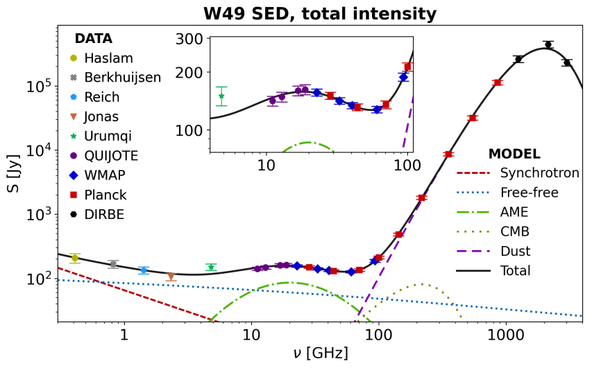
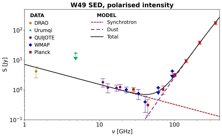
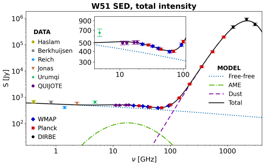
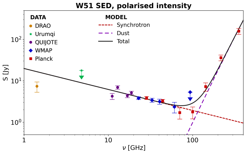
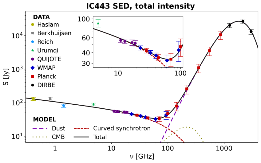
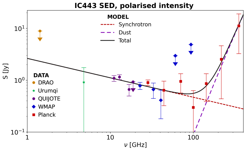
Figure 8: SEDs for W49, W51 and IC443, obtained from the combination of QUIJOTE and ancillary data, for the total intensity $I$ (left panels) and the total polarised intensity $P$ (right panels). The flux densities have been obtained via aperture photometry in a 1-degree radius aperture centred in the source, as detailed in Section 5, considering all maps smoothed at a 1 deg resolution. QUIJOTE points are the only available data for these regions covering the range between 10 and 20 GHz. Overplotted to the data point we show the best-fit models discussed in Section 6.2; the foregrounds considered for each fit are quoted in the plot legends. In total intensity the model plotted here for W49 is the one including a synchrotron component with a fixed spectral index (third column in Table 8), the model for W51 is the one with no synchrotron component (second column in Table 9), and for IC443 we show the model with a broken power-law synchrotron spectrum (last column of Table 10). When fitting for a dust component in the polarised SEDs, the dust temperature is always fixed to the value obtained in total intensity; for W51, the DRAO point was not included in the polarisation fit.

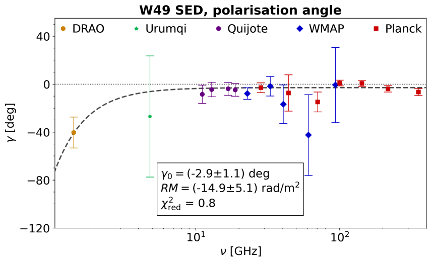
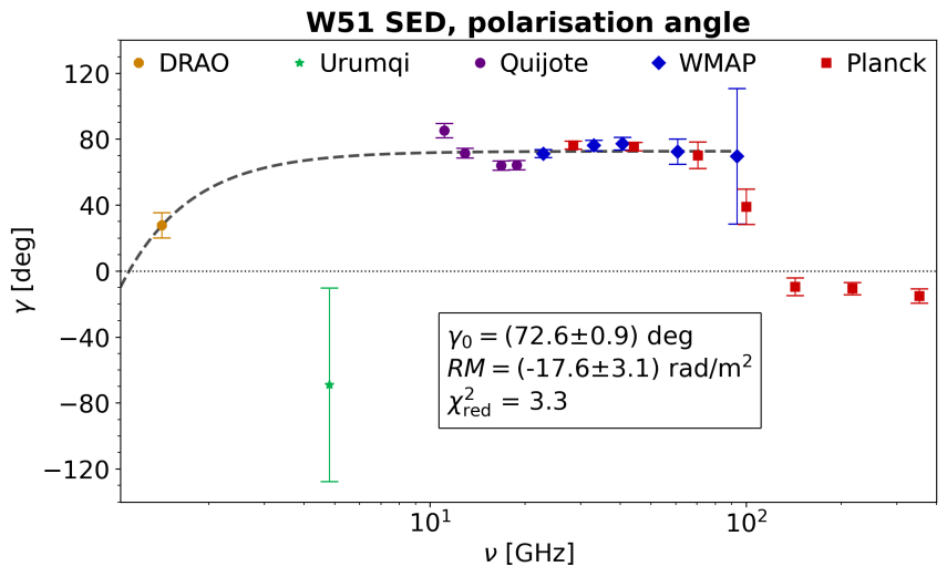
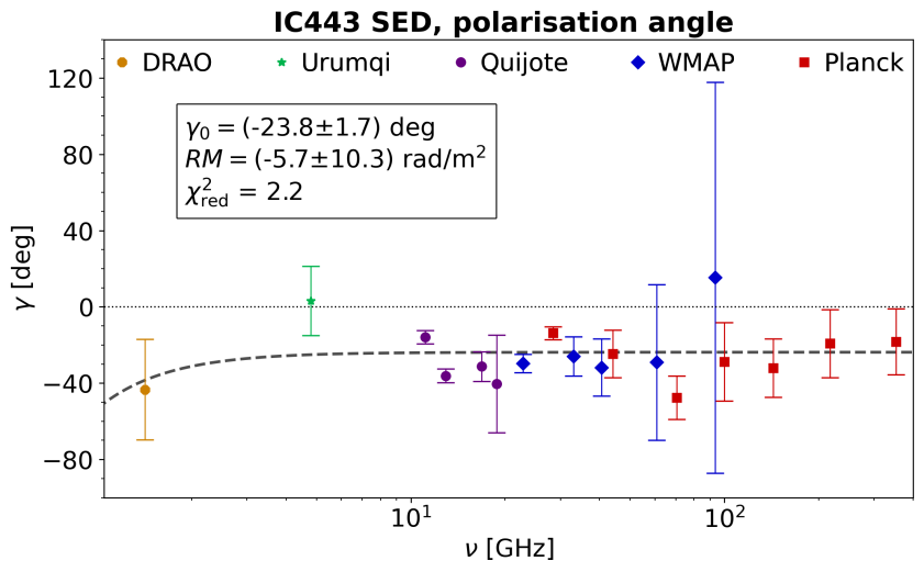
Figure 9: Polarisation angle $\gamma$ as a function of frequency, towards the three regions. We also overplot to the data points the best-fit Faraday rotation model from equation (9), and report the resulting parameter estimates in each panel.

6 Modelling the source emissions

This section is devoted to the physical interpretation of the flux densities measured towards the three sources considered in this work, taking into account both the total intensity and the polarisation SEDs.

6.1 Methodology

Our modelling of the source emissions considers the four continuum foreground mechanisms listed in Section 1. At low frequency, the contribution from the synchrotron emission is modelled with a power law:

$$S_{\rm sync}(\nu)=A_{\rm s}\left(\frac{\nu}{\nu_{\rm p}}\right)^{\alpha_{\rm s}},$$ (2)

with a pivot frequency $\nu_{\rm p}=1\,\text{GHz}$; we fit in this case for the synchrotron amplitude $A_{\rm s}$ at 1 GHz, and for the synchrotron spectral index $\alpha_{\rm s}$. We will consider the synchrotron contribution both in intensity and polarisation.

The free-free flux density as a function of frequency is given by (see for example Wilson et al., 2009):

$$S_{\rm ff}(\nu)=\frac{2k_{\rm B}\nu^{2}\Omega}{c^{2}}T_{\rm e}\left(1-e^{-\tau_{\rm ff}(\nu)}\right),$$ (3)

which is the radiation transfer equation for the free-free emission, with the first fraction representing the conversion factor between brightness temperature and flux density in the Rayleigh-Jeans limit; $k_{\rm B}$ is the Boltzmann constant, $c$ the speed of light, $T_{\rm e}$ the electron temperature and $\Omega$ the solid angle subtended by the chosen photometry aperture. All the information on the emission is encoded in the free-free opacity $\tau_{\rm ff}$, for which we adopt the parametrisation provided by Draine (2011):

$$\tau_{\rm ff}(\nu)=5.468\times 10^{-2}\left(\frac{T_{\rm e}}{\text{K}}\right)^{-1.5}\left(\dfrac{\nu}{\text{GHz}}\right)^{-2}\left(\frac{\text{EM}}{\text{pc}\,\text{cm}^{-6}}\right)g_{\rm ff}(\nu),$$ (4)

where the frequency $\nu$, the electron temperature $T_{\rm e}$ and the emission measure EM are expressed in convenient units, and $g_{\rm ff}$ is the Gaunt factor. For the latter we also choose the parametrisation given in Draine (2011), namely:

$$g_{\rm ff}(\nu)=$$

$$=\ln{\left[\exp{\left(5.960-\dfrac{\sqrt{3}}{\pi}\ln\left[Z\left(\dfrac{\nu}{\text{GHz}}\right)\left(\dfrac{T_{\rm e}}{10^{4}\,\text{K}}\right)^{-3/2}\right]\right)}+e\right]},$$ (5)

where $e$ is Napier’s constant and we set the charge number to $Z=1$ (hydrogen plasma). This modelling for the free-free emission is found to be more accurate than the conventional one (Wilson et al., 2009) over a broader frequency range, and was also employed in Planck Collaboration et al. (2014a). We want to fit for the value of the emission measure EM, which is defined as the squared electron density integrated along the line of sight and is generally adopted as an indicator of the strength of the free-free emission. Notice that it would not be possible to fit simultaneously for the emission measure and the electron temperature, given the strong degeneracy between the two parameters that is clear from equation (4). For the electron temperature we then adopt the values extracted from the public Planck COMMANDER free-free maps; more specifically, for each region we take the average of the $T_{\rm e}$ values found in the same aperture used to extract the flux density. We obtain the values $7000\,\text{K}$ for both W49 and W51, and $6861\,\text{K}$ for IC443.

The thermal emission from ISM dust grains is clearly evident in the FIR intensity SEDs for all regions. As customary, we model this emission as a modified blackbody, where in the optically thin regime the dust blackbody spectrum $B_{\nu}(T_{\rm dust})$ is weighted by the dust optical depth $\tau_{\text{dust}}$:

$$S_{\rm dust}(\nu) =\tau_{\text{dust}}(\nu)B_{\nu}(T_{\rm dust})\Omega=$$

$$=\tau_{\rm 250}\left(\frac{\nu}{1200\,\text{GHz}}\right)^{\beta_{\rm dust}}B_{\nu}(T_{\rm dust})\Omega.$$ (6)

In the second equality we expressed the frequency scaling for the dust opacity as a power law around a pivot frequency of 1200 GHz (or $250\,\mu\text{m}$). In this case we fit for the dust temperature $T_{\rm dust}$, emissivity $\beta_{\rm dust}$ and optical depth $\tau_{\rm 250}$ at $250\,\mu\text{m}$.

The AME emission is modelled phenomenologically as a parabola in the log-log plane (Stevenson, 2014):

$$S_{\rm AME}(\nu)=A_{\rm AME}\cdot\exp{\left\{-\frac{1}{2}\left[\frac{\ln({\nu/\nu_{\rm AME}})}{W_{\rm AME}}\right]^{2}\right\}}.$$ (7)

In this case we fit for the peak frequency $\nu_{\rm AME}$, the peak amplitude $A_{\rm AME}$ and the width of the parabola $W_{\rm AME}$. A similar form for the AME fitting function, although with a different meaning of the parameters, was proposed by Bonaldi et al. (2007), and employed in the previous QUIJOTE publications. Such a model, however, has the drawback of coupling the peak frequency and the width of the parabola (meaning that variations in $\nu_{\rm AME}$ would alter the value of $W_{\rm AME}$). The functional form from equation (7), instead, disentagles the parameters $\nu_{\rm AME}$ and $W_{\rm AME}$, which can now be varied independently.

Finally, we fit for a CMB contribution, expressed as the differential of the flux density with respect to the temperature times the CMB temperature fluctutation $\Delta T_{\rm CMB}$:

$$S_{\rm CMB}(\nu)=\dfrac{h^{2}\nu^{4}}{2k_{\rm B}T_{\rm CMB}^{2}c^{2}}\sinh^{-2}{\left(\dfrac{h\nu}{2k_{\rm B}T_{\rm CMB}}\right)}\,\Omega\,\Delta T_{\rm CMB},$$ (8)

where $h$ is the Planck’s constant and we adopt the reference CMB temperature $T_{\rm CMB}=2.7255\,\text{K}$ (Fixsen, 2009). In this case we fit for the value of $\Delta T_{\rm CMB}$.

The SED modelling is done with a Levenberg-Marquardt least-square fit (Markwardt, 2009) between our data points and the sum of the chosen foreground models, implemented via the Interactive Data Language (IDL) MPFITFUN function. As anticipated in Section 5, the model is used to compute colour correction coefficients for all frequencies above 10 GHz; these corrections are applied to the original flux densities and to their original uncertainties, and the fit is repeated, until convergence. The same procedure is adopted for both the intensity and polarisation SEDs. Before choosing the final model that best reproduces the SED of each source, we explore all different foreground combinations; this iterative correction process is applied consistently in each case.

Notice that the $\chi^{2}$ minimization performed in our fit assumes that all measurements are statistically independent. This is not entirely true for adjacent QUIJOTE frequencies belonging to the same horn, whose noise is correlated (see Rubiño-Martín et al., 2023, for a more complete discussion). We check for the effect this correlation can have on our source modelling in the following way. We combine the 11 and 13 GHz flux densities and errors into an effective 12 GHz measurement, using the correlation coefficients reported in Rubiño-Martín et al. (2023) when computing the effective uncertainty; the same procedure is repeated for the 17 and 19 GHz points, yielding and effective 18 GHz flux density estimate. When repeating the fit using this set of reduced QUIJOTE data, we find that the resulting best-fit parameters are compatible within their uncertainties with the full QUIJOTE data case. We therefore conclude that the existing noise correlations between adjacent QUIJOTE frequencies are negligible as far as our source modelling is concerned.

Information on the polarised emission can also be extracted from the frequency dependence of the polarisation angle shown in Fig. 9. Variations of $\gamma$ with frequency can be ascribed to Faraday rotation from the neighbouring ionised medium. The effect can be modelled, as a function of wavelength, as:

$$\gamma(\lambda)=\gamma_{0}+\text{RM}\,\lambda^{2},$$ (9)

where $\gamma_{0}$ is the polarisation angle for $\lambda=0$ (or $\nu\rightarrow\infty$) and RM is the rotation measure, which is proportional to the line-of-sight integral of the electron density times the parallel component of the magnetic field. We fit for $\gamma_{0}$ and RM over our measured $\gamma$ values, and report the best-fit estimates in each panel in Fig. 9. The resulting model for the polarisation angle is overplotted as a dashed line to the data.

6.2 Application to W49, W51 and IC443

The SEDs in total intensity shown in Fig. 8 can be modelled by a suitable combination of the four foregrounds mentioned in the beginning of this section. The contribution of thermal dust emission is clear in all the regions, producing the characteristic peak at FIR frequencies. The spectrum in the lowest frequency range shows a decrease which is due to either synchrotron or free-free emission, or a combination of the two. Any possible AME contribution would emerge in the microwave range as an excess signal with respect to the combination of synchrotron and the thermal emissions. The actual detection of AME towards these regions is then subject to a clear characterisation of the other foregrounds; this is particularly crucial for the low frequency points, where the free-free and synchrotron components are degenerate. For each region we will then repeat the fit by fixing the spectral index of the synchrotron power law to the value estimated from the polarised intensity SED, and fit only for its amplitude. We try different combinations of the four foreground emissions and finally quote the results that provide the best modelling of the measured SED; this is assessed evaluating both the resulting $\chi^{2}$ and the physical meaning of the best-fit parameter values. A summary of the fit results is reported in Tables 8, 9 and 10 for W49, W51 and IC443, respectively. The tables report the best-fit parameter values, the associated $\chi^{2}$ and the corresponding reduced chi-square defined as $\chi^{2}_{\rm red}=\chi^{2}/\text{dof}$, where the number of degree of freedom (dof) is computed as the number of fitted points minus the number of free parameters.

The polarised SEDs plotted in Fig. 8 show the joint contribution from a decaying component at low frequencies, and a raising component in the FIR range. The latter is to be ascribed to thermal dust emission, which is known to be polarised with fraction up to 20% in some regions of the sky (Planck Collaboration et al., 2020c); in our case the polarised flux densities suggest a low degree of polarisation, at the per cent level. The decaying part of the spectrum can be due either to free-free or to synchrotron. Although the former can yield a non-null residual polarisation fraction at the level $\lesssim 1\%$ (Trujillo-Bueno et al., 2002), as commented in Section 1 it is generally assumed a non-polarised foreground. The polarised signal observed towards our regions at low frequency is then most likely to be attributed to synchrotron emission.

In principle, we could adopt the functional forms from equations (2) and (6.1) and fit for a combination of the two foregrounds in polarisation. However, our FIR polarised flux densities only cover a portion of the rising dust spectrum, which is not effective in constraining the combination of the dust parameters. For this reason, we fix the dust temperature to the value obtained from the study of the corresponding SED in total intensity, and only fit for the dust emissivity and optical depth. Notice that we also considered a possible polarised AME contribution in our SED model, using the same functional form from equation (7). However, in all cases we found that the inclusion of a polarised AME component degrades the quality of the fit and yields non-physical values for the associated parameters. We conclude that there is no proof of any measurable AME polarised emission; as such, we decided not to include this foreground in the polarisation fit. The fit results for the three regions in polarisation are overplotted to the colour-corrected flux densities in the right panels of Fig. 8. In the fit we also kept the points that only provide upper limits on polarisation, by setting their flux density to zero and using their 1-$\sigma$ uncertainty.

6.2.1 W49

For W49, we find that the SED in intensity is best modelled by a combination of all the aforementioned components with the exception of synchrotron; the resulting best-fit parameter values are listed in Table 8. Our estimates for the free-free emission measure, the CMB temperature fluctuation and the thermal dust parameters are in agreement with those obtained in Planck Collaboration et al. (2014a). At low frequencies, the contribution from the free-free emission alone provides the best fit to the SED; when including a synchrotron component, the resulting best-fit spectral index is excessively steep ($\alpha_{\rm s}\simeq-1.3$) and its amplitude $A_{\rm s}$ is compatible with zero, so that we decided not to include a synchrotron contribution. Such a result can be understood, given that the bulk of the emission comes from the HII regions associated with W49A. The signal observed in polarisation towards W49 can be ascribed to the SNR W49B or, more likely, to the diffuse Galactic synchrotron emission; in any case, its contribution in total intensity is hindered by the brighter thermal bremmstrahlung coming from the star-forming regions. Hence, for simplicity, we decided not to include it in our source modelling; although we know that a synchrotron component is present, its inclusion yields non-physical results for its amplitude and spectral index, while only marginally changing the parameter values for the other emissions.

The situation is different when analysing the polarised SED, which clearly shows a decreasing spectrum at low frequencies that can be ascribed to synchrotron; we then fit the spectrum with a combination of synchrotron and thermal dust, fixing $T_{\rm dust}$ to the value obtained in total intensity. The resulting spectral index is $\alpha_{\rm s}=-0.67\pm 0.10$, which is consistent with the expected range for the synchrotron emission. It is then possible to try and fit for a synchrotron component in total intensity, fixing the spectral index to the value obtained in polarisation and only leaving the amplitude $A_{\rm s}$ as a free parameter. This time the synchrotron amplitude is detected at $2\,\sigma$, while the best-fit values for the free-free emission measure and the CMB temperature fluctuation have respectively a worse and better agreement with Planck Collaboration et al. (2014a); this can be expected as this reference does not include a synchrotron component in the source modelling, so that their free-free result accounts for the whole amplitude of the emission at low frequencies.

Table 8: Results of the multi-component fits for the W49 region. The table reports the best-fit values for different parameters when fitting the total intensity $I$ and the polarised intensity $P$. The table also reports the results of the fit in intensity when fixing the synchrotron spectral index to the value fitted in polarisation. When fitting for $P$ the dust temperature is always fixed to the value obtained in total intensity.

W49
Parameter	I	I (fixed $\alpha_{\rm s}$)	P
$A_{\rm s}$ [Jy]	-	65.3$\pm$31.3	7.2$\pm$2.2
$\alpha_{\rm s}$	-	-0.67	-0.67$\pm$0.10
EM [cm-6pc]	1315$\pm$84	774$\pm$283	-
$A_{\rm AME}$ [Jy]	55.0$\pm$7.2	85.9$\pm$17.6	-
$W_{\rm AME}$	0.6$\pm$0.1	0.9$\pm$0.2	-
$\nu_{\rm AME}$ [GHz]	21.0$\pm$1.4	20.0$\pm$1.4	-
$\Delta T_{\rm CMB}$ [$\mu$K]	98$\pm$67	174$\pm$88	-
$\tau_{250}\times 10^{3}$	1.52$\pm$0.26	1.53$\pm$0.27	0.03$\pm$0.01
$\beta_{\rm dust}$	1.75$\pm$0.09	1.75$\pm$0.10	1.64$\pm$0.13
$T_{\rm dust}$ [K]	20.4$\pm$0.9	20.4$\pm$0.9	20.4
$\chi^{2}$	12.3	8.9	16.8
$\chi^{2}_{\rm red}$	0.69	0.52	1.20

Still, the joint contribution of free-free, CMB and thermal dust is not enough to account for the microwave flux densities in total intensity, with QUIJOTE points clearly suggesting a downturn of the AME excess in this frequency range. We found that the inclusion of our AME functional form yields the best modelling with $\chi^{2}_{\rm red}=0.69$ without synchrotron and $\chi^{2}_{\rm red}=0.52$ when fixing $\alpha_{\rm s}$ (by comparison, a fit without AME would result in $\chi^{2}_{\rm red}=3.60$ and $\chi^{2}_{\rm red}=3.78$ respectively, with a flip in sign for the CMB temperature fluctuation). In the end, we can choose the modelling that includes the synchrotron with fixed spectral index as our reference model for W49, as it provides the best $\chi^{2}_{\rm red}$ value and yields physically reasonable values for all resulting parameters. The AME peak frequency is $\nu_{\rm AME}=20.0\pm 1.4\,\text{GHz}$, where it is detected with a significance of $\sim 4.7\sigma$ and accounts for $\sim 55\%$ of the observed intensity emission towards W49.

W49 does not appear in QUIJOTE maps as a strongly polarised source. In Fig. 2 it is visible in $Q$ as a local increase in the intensity of the polarised background, while there are only hints of positive $U$ towards the source. The flux densities quoted in Table 5 confirm this picture with most of the signal coming from positive $Q$. Since this polarised state is typical of the diffuse Galactic plane emission, the polarisation observed towards W49 may be produced by local intensification of the Galactic foreground, rather than by synchrotron emission proceeding specifically from the SNR W49B. The DRAO maps in Fig. 5 show a different configuration, in which the positive $Q$ towards the centre of the region is smeared, while $U$ shows a clear positive signal; this can be a result of Faraday rotation of the polarised direction showing up at the 21 cm wavelength. This observation is corroborated by the fact that the polarised intensity spectrum in Fig. 8 flattens at the lowest frequencies, suggesting a loss of polarised flux density (Faraday depolarisation). The $Q$ and $U$ flux densities in Table 5 show that this effect already begins to be important at the Urumqi 5 GHz frequency, although their high uncertainties only provide an upper limit for $P$, as shown in the SED plot. A more direct representation of this effect is provided by the spectral distribution of the polarisation angle in Fig. 9. While at $\nu\gtrsim 10\,\text{GHz}$ the angle is constantly close to zero, which means a mainly positive $Q$ state, the DRAO and Urumqi points show a deviation that can be fitted by our Faraday rotation model with a rotation measure $RM=(-14.9\pm 5.1)\,\text{rad}/\text{m}^{2}$. We stress that, although we measure a Faraday rotation effect, the associated synchrotron emission likely does not proceed from the SNR W49B, but rather from the diffuse Galactic polarised emission; as a further proof of this, we notice that the peak of the positive U emission in the DRAO map is shifted with respect to the position of W49. Nonetheless, as this polarised signal is captured by our aperture, it is worth showing the associated modelling in $P$ and $\gamma$ as part of our study of QUIJOTE data towards this region.

6.2.2 W51

For W51 the situation is very similar to W49: the local massive molecular clouds and associated HII regions are the main source of radio emission at low frequencies, where they mask the non-thermal emission from the SNR W51C. The SED is best fitted by a combination of free-free, AME, CMB and thermal dust, with the estimates on the parameters reported in Table 9; the CMB in this case shows a negative contribution, which however is compatible with zero. Our dust parameters are in reasonably good agreement with the ones reported in Demetroullas et al. (2015), considering that their fit includes a synchrotron component and does not include AME or CMB. In our fit, the inclusion of AME determines a considerably better agreement between the model and the data points, improving the $\chi^{2}_{\rm red}$ value from 2.06 to 1.23. The inclusion of a synchrotron component, instead, would make the free-free emission measure compatible with zero and yield non-physical values for the AME parameters; when keeping the synchrotron and removing the AME component we find again a free-free amplitude compatible with zero and a very flat synchrotron spectrum ($\alpha_{\rm s}\simeq-0.1$). We therefore decided not to include the synchrotron component in our intensity fit.

However, unlike W49, W51 clearly stands out against the Galactic plane as a bright polarised source, with both negative $Q$ and $U$. Among the three regions considered in this work, it is the one that provides the highest polarised flux densities; still, this increase in the polarised flux density is associated with an increase in the total intensity towards the source, so that the resulting polarisation fractions in Table 6 are at the same level as for the other regions. Also, for W51 the effect of Faraday depolarisation appears even stronger than in the case of W49: this can be seen already from the Urumqi and DRAO maps in Fig. 5. The screening effect is likely due to intervening ionised gas along the line of sight towards W51C, possibly associated with the HII regions from the neighbouring W51A. As reported in Table 6, at the Urumqi frequency the $U$ flux density is compatible with zero, while the polarised SED in Fig. 8 shows that the DRAO point flux density is at the same level as the lowest QUIJOTE frequencies. The spectral distribution of the polarisation angle shown in Fig. 9 once again confirms this picture, with a rather constant angle at microwave frequencies and a sharp decrease at $\nu\lesssim 10\,\text{GHz}$. The fit of our Faraday rotation model yields $RM=(-17.6\pm 3.1)\,\text{rad}/\text{m}^{2}$, which is higher in modulus than the estimate obtained for W49, confirming the effect is more relevant. Note that in this case we did not include the Planck-HFI points in the fit, as in the plot they show a break with the microwave trend; this is probably due to polarised dust contribution, either from the diffuse Galactic background or associated with the HII regions in W51. The effect is also quite evident from the bottom row panels in Fig. 5.

Table 9: Same as in Table 8, but for the W51 region.

W51
Parameter	I	I (fixed $\alpha_{\rm s}$)	P
$A_{\rm s}$ [Jy]	-	359.0$\pm$140.3	19.8$\pm$4.6
$\alpha_{\rm s}$	-	-0.51	-0.51$\pm$0.07
EM [cm-6pc]	2828$\pm$178	428$\pm$1071	-
$A_{\rm AME}$ [Jy]	105.6$\pm$26.3	359.3$\pm$121.7	-
$W_{\rm AME}$	0.9$\pm$0.3	1.7$\pm$0.4	-
$\nu_{\rm AME}$ [GHz]	17.7$\pm$3.6	15.8$\pm$3.0	-
$\Delta T_{\rm CMB}$ [$\mu$K]	-51$\pm$105	94$\pm$181	-
$\tau_{250}\times 10^{3}$	1.08$\pm$0.20	1.10$\pm$0.21	0.03$\pm$0.02
$\beta_{\rm dust}$	1.65$\pm$0.10	1.66$\pm$0.11	2.35$\pm$0.33
$T_{\rm dust}$ [K]	23.1$\pm$1.2	22.9$\pm$1.3	23.1
$\chi^{2}$	22.2	19.2	29.2
$\chi^{2}_{\rm red}$	1.23	1.13	2.25

Once again, the polarised SED is best fitted by a combination of a synchrotron and a thermal dust component alone. Including all our available points we obtain the values $\alpha_{\rm s}=-0.37\pm 0.05$ and $S_{\rm sync}^{\rm 1\,\text{GHz}}=12.7\pm 2.0$ with $\chi^{2}_{\rm red}=2.61$. Demetroullas et al. (2015) obtained the estimate $\alpha_{\rm s}=-0.58\pm 0.06$ when using CBI 31 GHz and Effelsberg 2.7 GHz data. Our flatter spectrum can be a result of Faraday depolarisation at the lowest frequencies, as explained. In fact, if we remove the DRAO point from the fit and only keep frequency points from 4.8 GHz upwards (the Urumqi point only providing an upper limit), we obtain the values reported in Table 9, with the compatible estimate $\alpha_{\rm s}=-0.51\pm 0.07$. We conclude that the Faraday depolarisation severely affects the DRAO point, in such a way that its inclusion in the fit would result in a biased estimation of the synchrotron spectral index. Hence, we keep the fit results obtained removing the DRAO point as our fiducial estimates.

Going back to the intensity SED, we still tried to include a synchrotron component by fixing its spectral index to the value $\alpha_{\rm s}=-0.51$ fitted in polarisation. Although the goodness of fit is maintained ($\chi^{2}_{\rm red}=1.13$) this modification in the modelling significantly alters the values of the emission measure (which is now compatible with zero), the CMB (again compatible with zero but positive) and the AME parameters, the latter showing an unphysically large value for $W_{\rm AME}$, and a very low value for the peak frequency. We also tried and fixed the synchrotron amplitude too, by assuming a polarisation fraction of 20%; from the polarisation best-fit modelling, this results in $A_{\rm s}=99\,\text{Jy}$. When fixing both the synchrotron amplitude and spectral index, compared to the case of no synchrotron, we obtain compatible best-fit parameters for the thermal dust, a slightly larger value for the emission measure $\text{EM}=(2246\pm 250)\,\text{pc}\,\text{cm}^{-6}$, a sign-flipped CMB contribution (still compatible with zero) $\Delta T_{\rm CMB}=(6\pm 121)\,\mu K$ and AME parameters equal to $A_{\rm AME}=(164\pm 36)\,\text{Jy}$, $W_{\rm AME}=1.2\pm 0.4$ and $\nu_{\rm AME}=(16.8\pm 3.4)\,\text{GHz}$, with $\chi^{2}_{\rm red}=1.15$. Although the AME width is still rather large, this example shows that the observed SED in intensity is in fact compatible with the inclusion of a synchrotron component at reasonable levels; however, we do not adopt this fit as our fiducial model for W51 due to the rather arbitrary value we assigned to the polarisation fraction. In conclusion, the intensity SED suggests that although a synchrotron component is present in the source emission, the observed low-frequency data are best modelled by a free-free component alone, which is by far the dominant foreground emission mechanism in this frequency range. The inclusion of the AME component, on the contrary, always improves the quality of this fit, changing the $\chi^{2}_{\rm red}$ from $2.17$ to $1.13$ (from $3.05$ to $1.15$ when the synchrotron amplitude is also fixed). For all these considerations, we fix the combination of free-free, AME, CMB and thermal dust, with no synchrotron, as the best model for W51 in total intensity. Towards this region AME is detected at the peak frequency $\nu_{\rm AME}=(17.7\pm 3.6)\,\text{GHz}$ with a significance of $\sim 4.0\,\sigma$, contributing to the observed intensity emission with a $\sim 21\%$ in flux density. Its relative significance, then, is lower compared to W49.

6.2.3 IC443

In total intensity IC443 shows a different combination of emission mechanisms compared to the other two sources. In this case, we find that the best-fit model consists of synchrotron (with spectral index $\alpha_{\rm s}=-0.29\pm 0.03$), free-free, CMB and thermal dust, with the parameters reported in the second column of Table 10 and a final $\chi^{2}_{\rm red}=0.73$. Any combination that does not include a synchrotron component would result in values of $\chi^{2}_{\rm red}>2$, non-physical values for most parameters and an overall bad agreement between the model and the points at low frequency. This proves that the bulk of the IC443 emission is non-thermal and proceeds from the local SNR. On the contrary, a model without a free-free component could be valid as well, yielding $\chi^{2}_{\rm red}=0.69$ and values for the other parameters compatible with those reported in the second column of Table 10. Thermal bremmstrahlung radiation from IC443 was initially claimed in Onić et al. (2012), although discarded by subsequent work; it is clear that free-free is a subdominant component in this region, but its presence cannot be discarded a priori. Since it is detected in our fit with reasonable values for the other parameters, it is worth including it in the source modelling. On the contrary, the inclusion of AME as an additional component would yield $\chi^{2}_{\rm red}=0.80$, with quite low values for the AME amplitude ($A_{\rm AME}=4.4\pm 3.8\,\text{Jy}$), width ($W_{\rm AME}=0.21\pm 0.19$) and peak frequency ($\nu_{\rm AME}=16.3\pm 2.7$); similar considerations hold when the CMB contribution is removed from the fit. We conclude that the measured SED in IC443 does not provide any compelling evidence for the presence of AME towards the region. We stress that dust emission towards IC443 is well-reconstructed, but its amplitude is at least one order of magnitude lower compared to W49 and W51. This suggests a limited presence of dust in the region; as AME is generally observed in association with dust, it is not likely to be observed towards IC443.

IC443 is detected in polarisation across our microwave frequencies as a positive $Q$ and $U$ source. The low dust amplitude in total intensity also results in very low flux densities in polarisation; even at lower frequencies, the flux densities in $Q$ and $U$ are often consistent with zero. In this case the debiasing employed to compute $P$ flux densities is important to prevent overestimating the polarised intensity. Still, although the microwave polarised flux densities are generally below 1 Jy, in this case the position of the source outside the Galactic plane allows the detection of its polarised emission with less confusion with the background. Most likely, this polarised signal is synchrotron emission from the SNR, and it is reasonable to fit for the corresponding power law on the polarised SED. At 1.4 GHz the source still yields a positive $U$ flux density, and a value of $Q$ consistent with zero; the DRAO maps in Fig. 6 show hints of positive polarisation signal towards the centre of the aperture, although being in general subdominant with respect to other background structures. At 5 GHz the source yields a strong positive $Q$ flux density, and a change of sign in $U$. These considerations may indicate that the two lowest frequency points are once again affected by Faraday rotation, although their error bars are too large to firmly establish it. In fact, looking at the SEDs plot in Fig. 8, there seems not to be a net flux density loss below 10 GHz, and the spectrum decays as expected for a synchrotron emission. As a further confirmation, we can see from Fig. 9 that in this case the variation of the polarisation angle at low frequency is very mild, and as a result our Faraday rotation fit yields a value of $RM=(-5.7\pm 10.3)\,\text{rad}/\text{m}^{2}$ for the rotation measure, which is compatible with zero and considerably lower in modulus than the one measured for W49 or W51. We thus conclude that, although we observe hints of Faraday rotation towards IC443, the effect is negligible as far as our analysis is concerned. We therefore proceed with a fit for the polarised SED using all available points, and modelling again the emission as a combination of synchrotron and dust; the resulting parameters are reported in the fourth column of Table 10, with a synchrotron spectral index of $\alpha=-0.37\pm 0.13$ and $\chi^{2}_{\rm red}=0.90$.

Going back to the SED in total intensity, when fixing the synchrotron spectral index to the value obtained in polarisation, we find the best-fit is obtained with the same model adopted when the synchrotron spectral index was left free, i.e. a combination of synchrotron, free-free, CMB and thermal dust. Compared to the case of free spectral index, the synchrotron amplitude decreases while the measurement of the free-free emission measure becomes more significant; the parameter values associated with CMB and thermal dust, instead, are only marginally affected (third column of Table 10). Once again, the inclusion of AME would yield non-physical values for the associated parameters, especially for its peak frequency ($\nu_{\rm AME}\simeq 6\,\text{GHz}$). The fact that the free-free amplitude is higher in this case can be the result of a steepening of the synchrotron spectrum at frequencies above a few GHz. In that case, because the synchotron is fitted in polarisation starting from $\sim 5\,\text{GHz}$ (the DRAO point really only provides an upper limit), we would expect the value of $\alpha_{\rm s}$ to be larger in modulus compared to the result fitted in total intensity. When forcing such a steep spectrum in the intensity SED, the fit better accommodates the lowest frequency points by lowering the synchrotron amplitude and including a flatter spectral contribution as is the one from the free-free emission. So, our detection of thermal emission in IC443 may simply be a result of an inaccurate modelling of the synchrotron spectrum across the frequency range we explore.

In order to better test this hypotesis, we also try and fit for a curved synchrotron model, which differs from the parametrisation in equation (2) for the inclusion of a cut-off frequency $\nu_{\rm 0,s}$:

$$S_{\rm sync}^{\rm curv}(\nu)=A_{\rm s}\left(\frac{\nu}{\nu_{\rm p}}\right)^{\alpha_{\rm s}}\,\exp{\left(-\dfrac{\nu}{\nu_{\rm 0,s}}\right)}.$$ (10)

With this model, we find that the best fit to the IC443 intensity spectrum is provided by a combination of synchrotron, CMB and thermal dust, with the best value of $\chi^{2}_{\rm red}=0.61$ obtained for this region and a spectral index which is lower in modulus than one obtained for a simple power-law synchrotron model (last column of Table 10). In this case the CMB component flips sign compared to the case of the simpler synchrotron model, although its amplitude is compatible with zero, confirming that it is a subdominant component in the SED. The inclusion of AME generally yields unphysical values for its parameters, and the inclusion of free-free results in too low a value for the synchrotron cut-off frequency (around 60 GHz). We then decided to fit IC443 as a combination of curved synchrotron, CMB and thermal dust; this is the model that is overplotted to the data points in Fig. 8, and the resulting parameters are quoted in the fifth column of Table 10.

Table 10: Same as in Table 8, but for the IC443 region. In this case, the additional last column reports the results of the fit which adopts a broken power-law synchrotron model, and which results in the best modelling for IC433 intensity SED.

IC443
Parameter	$I$	$I$ (fixed $\alpha_{\rm s}$)	$P$	$I$ (curv. s.)
$A_{\rm s}$ [Jy]	96.5$\pm$10.6	71.9$\pm$10.9	2.6$\pm$1.0	106.7$\pm$5.8
$\alpha_{\rm s}$	-0.29$\pm$0.03	-0.37	-0.37$\pm$0.13	-0.21$\pm$0.04
$\nu_{\rm 0,s}$ [GHz]	-	-	-	114$\pm$73
EM [cm-6pc]	69$\pm$60	235$\pm$39	-	-
$\Delta T_{\rm CMB}$ [$\mu$K]	-58$\pm$37	-65$\pm$35	-	29$\pm$54
$\tau_{250}\times 10^{3}$	0.09$\pm$0.03	0.09$\pm$0.03	0.002$\pm$0.006	0.11$\pm$0.04
$\beta_{\rm dust}$	1.31$\pm$0.25	1.28$\pm$0.23	2.12$\pm$1.49	1.51$\pm$0.29
$T_{\rm dust}$ [K]	20.6$\pm$2.0	20.7$\pm$1.9	20.0	19.4$\pm$1.9
$\chi^{2}$	13.1	13.8	12.7	11.0
$\chi^{2}_{\rm red}$	0.73	0.72	0.90	0.61

Previous works already tackled the modelling of IC443 spectrum from radio to FIR frequencies. As already mentioned, Onić et al. (2012) claimed the detection of free-free towards the region, accounting up to 57% of the observed emission at 1 GHz. Our model with a free spectral index results in a free-free amplitude of $\sim 10\,\text{Jy}$, or $\sim 10\%$ of the total, while the fixed spectral index model yields $\sim 36\,\text{Jy}$, or $\sim 33\%$ of the total; both these estimates are in agreement with the quoted result. We already stressed, however, how our finding could be simply the result of forcing too steep a synchrotron spectrum. In Planck Collaboration et al. (2016a) the existence of a thermal component was ruled out, and IC443 was modelled as a simple combination of synchrotron and thermal dust; for the latter, they quote $\beta_{\rm dust}=1.5$, in agreement with our finding, and $T_{\rm dust}=16\,\text{K}$, which is $\sim 2\sigma$ lower than our estimate (although the reference does not quote error bars, which makes an acutal comparison unreliable). As per the synchrotron, they favour $\alpha_{\rm s}=-0.36$, compatible with our estimate in polarisation, although they mention that for frequencies above 40 GHz the spectrum shows a steepening to $\alpha_{\rm s}=-1.5$. This observation corroborates our use of a curved synchrotron model. In Onić et al. (2017) the IC443 SED from 400 MHz to 143 GHz was fitted using a combination of synchrotron, thermal dust and AME (not favouring any free-free contribution). Their work also stressed the presence of a break in the synchrotron power law visible above $\sim 5\,\text{GHz}$, and they also considered a curved synchrotron model as in our equation 10. Different implementations pointed towards a cut-off frequency in the range $112\,\text{GHz}<\nu_{\rm 0,s}<152\,\text{GHz}$ and spectral index in the range $-0.39<\alpha_{\rm s}<-0.35$; their estimates for the dust temperature are in agreement with Planck results, while their emissivity results are slightly higher, in the range $1.97<\beta_{\rm dust}<2.345$. Most importantly, they detected an excess of emission at 30 GHz which they interpreted as AME. A very similar analysis was conducted in Loru et al. (2019), measuring a curved synchrotron with $\alpha_{\rm s}=-0.38$ and $\nu_{\rm 0,s}=(148\pm 23)\,\text{GHz}$, and claiming a detection of AME peaking at $\nu_{\rm 0,AME}=(28\pm 3)\,\text{GHz}$. The synchrotron cut-off frequency obtained in our analysis is consistent with these results.

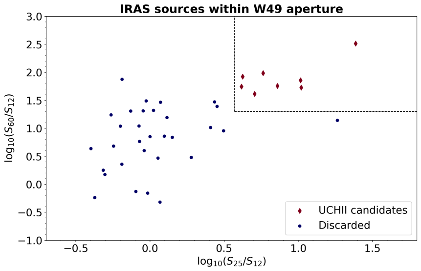
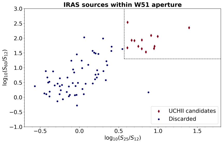
Figure 10: Extraction of candidate UCHII regions using IRAS data for both W49 (left panel) and W51 (right panel). Points represent IRAS galactic IR sources entering the aperture employed for the photometric study of each region, displayed in a colour-colour plot based on IRAS measured flux densities. UCHII regions are expected to yield ratios $\log_{10}{(S_{60}/S_{12})}\gtrsim 1.30$ and $\log_{10}{(S_{25}/S_{12})}\gtrsim 0.57$; the group of sources satisfying these condition is shown with red diamonds, with the dashed lines marking the flux density boundaries. In this way we select 8 sources for W49 and 13 sources for W51, and use them to estimate the contamination from UCHII to our AME detections. See Section 6.3.1 for details.

Although these previous works would agree in establishing the presence of AME towards IC443, there are some issues that should be pointed out. First of all, their analyses rely on the combination of flux density estimates coming from previous results in the literature, obtained using different types of radio observations, different angular resolutions and different analysis techniques. Although Onić et al. (2017) recognised the inherent risks of such an approach, which makes their study somehow qualitative, they still firmly established the need for an extra emission at microwave frequencies to account for the observed excess. Besides, both Onić et al. (2017) and Loru et al. (2019) adopted the microwave flux densities from Planck Collaboration et al. (2016a). Those flux densities were measured with aperture photometry, adopting a variable size of the aperture as a function of the considered frequency. The analysis in Planck Collaboration et al. (2016a) introduced a correction factor, equal to 1.4 for IC443, to account for the loss of flux density that is not captured inside their aperture due to the beam convolution. The authors did not applied this correction to well-resolved sources, defined as those with diameter 50% larger than the beam FWHM. As the Planck beam FWHM decreases with increasing frequency, this criterion implies that for IC443 the correction is applied at 30 and 44 GHz, but not from 70 GHz onwards. Their analysis adapted the size of the aperture at each frequency, in such a way that the same fraction of flux density should be retained inside the aperture; hence, these correction factors should be applied to all their frequency points, and not only to 30 and 44 GHz. This approach produces an artificial dip of the SED at 70 GHz, which the authors interpreted as the downturn of AME. We can also argue that this strategy for the flux density extraction is not appropriate in cases of significant background fluctuations, as it is the case for IC443; in fact, none of those works adopted any masking around IC443, so that the aperture photometry estimation of the flux density emission and/or the background level can be easily biased by the contribution from the neighbouring sources Sh2-249 and Sh2-252. The analysis we have presented in this paper, however, not only took care of the mask, but also measured the flux densities adopting a common angular resolution and a consistent methodology (with fixed apertures and background annuli) that is applied throughout the considered frequency range. In conclusion, we do believe that the available data set points towards an absence of AME emission towards IC443; at the very least, we can affirm that if an AME component is present, it is dominated by the uncertainties in our flux density measurements, and is certainly much fainter than the emission detected towards W49 and W51. Although we still observe a dip in the IC443 spectrum around 70 GHz, it can be more reasonably fitted with a curved synchrotron component, and is not sufficently compelling to justify the inclusion of AME at $\sim 30\,\text{GHz}$.

6.3 Further considerations on AME

We conclude our analysis by commenting some further aspects related to the detection of AME in W49 and W51. First of all, we have to stress that, because we are working with maps smoothed at a 1-degree angular resolution and we use apertures of typical radius of $\sim 1\,\text{deg}$, the measured flux densities may have a significant contribution from the region neighbouring each source. Therefore, although we detect AME towards W49 and W51, it is hard to assess whether the measured signal proceeds entirely from the sources or has an important contribution from the diffuse Galactic emission in their surroundings. Although in the rest of this section we will still discuss about AME emission from W49 and W51, it is important to acknowledge this possibility. Further discussion about this matter can be found in Appendix A.

6.3.1 Contribution from ultra-compact HII regions

UCHII regions are produced by recently formed massive stars which are still embedded in their molecular clouds; those with $\text{EM}\gtrsim 10^{7}\,\text{cm}^{-6}\text{pc}$ can have a significant optically thick free-free emission at frequencies up to 10 GHz or higher. This emission can produce an excess in the measured flux density at QUIJOTE frequencies, thus mimicking the effect of AME on the SEDs of W49 and W51. The goal of this section is to assess to what extent the contribution from UCHII can affect the significance of our AME detection.

At first we follow the procedure described in Planck Collaboration et al. (2014a) and also adopted by Poidevin et al. (2023), to which we redirect for a more detailed explanation and further references. This method is based on the extraction of candidate UCHII sources entering our chosen apertures and on the estimation of their total flux density at AME frequencies. For this we employ data from the IRAS Point Source Catalogue, which provides flux density measurements for point sources at 12, 25, 60, and 100$\,\mu\text{m}$. For both W49 and W51 we query the catalogue to extract the IR sources contained in the aperture employed for our photometric flux density measurements; in addition, we discard sources which are extragalactic or upper limits in either $25\,\mu\text{m}$ or $60\,\mu\text{m}$. We then place the retrieved IR sources on a $\log_{10}{(S_{25}/S_{12})}$–$\log_{10}{(S_{60}/S_{12})}$ plane as shown in Fig. 10, where $S_{x}$ denotes the IRAS measured flux density at wavelength $x$. UCHII sources are expected to have $\log_{10}{(S_{60}/S_{12})}\gtrsim 1.30$ and $\log_{10}{(S_{25}/S_{12})}\gtrsim 0.57$; as marked in Fig. 10, this leaves 8 IR sources in W49 and 13 sources in W51. IRAS data allow to evaluate the associated total flux density at 100 $\mu\text{m}$. For an UCHII region, the ratio between this flux density and the flux density at 15 GHz is found to lie in the range 1000-400000, which allows us to place both an upper and a lower limit to the expected UCHII contamination at QUIJOTE frequencies. The results are reported in Table 11, where they are compared with the residual AME amplitudes at the same frequency. We see that in the worst case scenario the contribution from UCHII sources can account for $\sim 55\%$ of the AME flux density towards W49, and for $\sim 32\%$ of the AME flux density towards W51. We stress that this not only is an upper limit, but according to Planck Collaboration et al. (2014a) it is also likely overestimated by a factor of a few. The corresponding lower limit estimate is completely negligible compared to the measured AME flux density, which confirms our detection of AME cannot be ruled out on the basis of this simple extrapolation.

In order to get an independent estimate of the possible contamination from UCHII regions, we consider data from the CORNISH continuum survey of the Galactic plane at 5 GHz with a 1.5 arcsec resolution (Purcell et al., 2013). CORNISH legacy data include a catalogue of identified UCHII regions, which we query to select the ones entering our apertures. We find 24 sources within the W49 aperture and 8 sources within the W51 aperture, contributing with the 5 GHz flux densities quoted in Table 11. Now, there is no standard way to extrapolate these flux densities to the peak frequency of our AME detection. Nonetheless, we can refer to the SEDs plotted in Kurtz et al. (1994) for several different UCHII regions, which were built using VLA integrated flux density measurements at 8.3 and 15 GHz in combination with IRAS flux densities and other ancillary data. The plots do not show any appreciable variation of the spectrum for frequencies $\lesssim 100\,\text{GHz}$. Hence, to a first approximation we can extrapolate our UCHII flux density measurements at 5 GHz to 15 GHz for a comparison with the corresponding AME residuals. We find that the contribution from UCHII amounts to $\sim 10\%$ of the AME amplitude in W49 and to $\sim 5\%$ in W51. We conclude that, although a non-negligible contribution from UCHII is entering our measured flux densities, it is not enough to account for the local SED excess amplitude and rule out the presence of AME. Novel, tailored observations to these regions are required to better constrain the UCHII contribution.

Table 11: Results for the contribution from UCHII regions in W49 and W51. We report the AME residual amplitude at 15 GHz, $S_{\rm 15GHz}^{\rm AME}$, the measured UCHII total flux at 100 $\mu$m from IRAS data, $S_{100\mu\text{m}}^{\rm IRAS}$, and its corresponding upper and lower limit extrapolations at 15 GHz, $S_{15\text{GHz}}^{\rm uplim}$ and $S_{15\text{GHz}}^{\rm lowlim}$. The last column reports the total UCHII flux measured with CORNISH data at 5 GHz.

Source	$S_{\rm 15GHz}^{\rm AME}$	$S_{100\mu\text{m}}^{\rm IRAS}$	$S_{15\text{GHz}}^{\rm uplim}$	$S_{15\text{GHz}}^{\rm lowlim}$	$S_{\rm 5GHz}^{\rm CORNISH}$
	[Jy]	[Jy]	[Jy]	[Jy]	[Jy]
W49	81.4	45098	45.1	0.1	8.5
W51	103.9	33368	33.4	0.1	5.3

Table 12: AME polarisation constraints from 16 to 61 GHz. For each frequency point we report the local residual AME amplitude $I_{\rm AME}$, the colour-corrected polarised flux $P$, the resulting polarisation fraction $P/I_{\rm AME}$ and the associated upper limit for the AME polarisation fraction $\Pi_{\rm AME}$, computed as the 95% confidence level upper boundary on the fraction $P/I_{\rm AME}$. When no uncertainty on $P/I_{\rm AME}$ is quoted it means the debiased $P$ flux is null and the reported upper limit is already the top boundary of the 95% confidence level.

W49
Freq.	$I_{\rm AME}$	$P$	$P/I_{\rm AME}$	$\Pi_{\rm AME}$
[GHz]	[Jy]	[Jy]	[%]	[%]
16.8	84.2$\pm$17.3	1.2$\pm$0.3	1.4$\pm$0.4	$\lesssim$2.3
18.8	85.7$\pm$17.5	1.2$\pm$0.3	1.5$\pm$0.4	$\lesssim$2.3
22.8	84.9$\pm$17.5	1.0$\pm$0.2	1.2$\pm$0.4	$\lesssim$1.9
28.4	79.2$\pm$17.2	1.0$\pm$0.2	1.3$\pm$0.4	$\lesssim$2.0
33.0	72.8$\pm$16.9	0.8$\pm$0.3	1.0$\pm$0.5	$\lesssim$2.0
40.6	61.7$\pm$16.6	0.4${}^{+0.2}_{-0.4}$	0.6${}^{+0.4}_{-0.7}$	$\lesssim$1.4
44.1	56.8$\pm$16.5	0.3$\pm$0.2	0.6${}^{+0.3}_{-0.4}$	$\lesssim$1.2
60.8	38.0$\pm$15.0	$\lesssim$1.2	$\lesssim$3.1	$\lesssim$3.1
W51
Freq.	$I_{\rm AME}$	$P$	$P/I_{\rm AME}$	$\Pi_{\rm AME}$
[GHz]	[Jy]	[Jy]	[%]	[%]
16.8	105.5$\pm$27.5	4.4$\pm$0.4	4.1$\pm$1.2	$\lesssim$6.4
18.8	105.4$\pm$28.0	5.1$\pm$0.5	4.9$\pm$1.4	$\lesssim$7.6
22.8	101.7$\pm$29.9	3.8$\pm$0.3	3.8$\pm$1.1	$\lesssim$6.0
28.4	92.7$\pm$32.1	3.9$\pm$0.3	4.2$\pm$1.5	$\lesssim$7.1
33.0	84.2$\pm$32.6	3.4$\pm$0.4	4.1$\pm$1.6	$\lesssim$7.3
40.6	70.6$\pm$32.0	3.2$\pm$0.5	4.5$\pm$2.1	$\lesssim$8.7
44.1	64.9$\pm$31.4	3.3$\pm$0.3	5.1$\pm$2.5	$\lesssim$10.1
60.8	43.4$\pm$27.6	2.3$\pm$0.7	5.4$\pm$3.8	$\lesssim$12.9

6.3.2 Constraints on AME polarisation

One of the driving goals of this analysis was the search for a possible polarised AME emission, which has not been detected to date and could shed light on the mechanism responsible for this foreground (Section 1). We have already commented that for both W49 and W51 the polarised SED is suitably modelled by a combination of synchrotron emission and dust emission alone. Although AME is not directly detected in our polarisation fits, we can proceed in a way similar to what was done in Génova-Santos et al. (2017) and Poidevin et al. (2019) to quote upper limits for the AME polarisation fraction.

We proceed as follows. We consider the frequency points where AME is most significant and less affected by other foregrounds, i.e. those in the frequency range from 17 GHz to 61 GHz. In this frequency range we generate a set of 1000 AME residual SEDs in intensity, computed using equation (7) and adopting random AME parameters; the latter are sampled from a Gaussian distribution centred on the best-fit estimates from Tables 8 and 9, and scattered according to their uncertainties. The dispersion of these realisations at the chosen frequency points allows to evaluate the uncertainty for the local AME intensity $I_{\rm AME}$. The resulting flux densities are quoted in Table 12, together with the polarised $P$ flux densities at the same frequencies. We then compute the associated polarisation fractions as $P/I_{\rm AME}$, which are reported in the fourth column of Table 12 in percent units.

Clearly, we know that at these frequencies an important polarised contribution comes from both the synchrotron and the dust emission. These fractions should therefore be interpreted as upper limits on the AME polarisation fraction. In fact, while the AME intensity peaks around 20 GHz, the polarised flux densities steadily decrease over the considered frequency range, and are most likely associated with synchrotron. For this reason, in the last column of Table 12 we report explicitly the upper limits on the AME polarisation fraction $\Pi_{\rm AME}$, which are computed as the 95% confidence level upper boundaries of the $P/I_{\rm AME}$ values. We can quote the tighest constraints $\Pi_{\rm AME}\lesssim 1.2\%$ for W49 at 44.1 GHz and $\Pi_{\rm AME}\lesssim 6.0\%$ for W51 at 22.8 GHz. The constraint for W51 is quite loose and does not allow to provide any strong claim on the nature of AME; the constraint for W49 is instead tighter, and favours the spinning dust model as the most plausible physical mechanism for AME. Follow up studies of W49 and W51 with higher resolution are required to better characterise their polarised emission, as the contamination from the observed polarised synchrotron is still the major factor hampering the measurement of a real AME polarised upper limit towards these region.

We conclude this section acknowledging that our polarisation fractions may be underestimated, as the integration of the Stokes parameters inside the apertures may result in depolarisation. To check for this effect, we can try and evaluate the level of possible aperture depolarisation effects on the dust flux densities; we consider the Planck 353 GHz map, where the dust polarisation flux densities are the highest. We then compute the (debiased) polarised intensity $P$ for individual pixels in the region surrounding W49 and W51, and obtain a new estimate on the polarisation of these sources by applying aperture photometry directly on the $P$-map. For clarity, we shall label these new polarised flux densities as $P^{\rm(pix)}$, to stress that they are obtained integrating the values of individual pixels, while we refer to the flux densities we employed up to now as $P^{\rm(ap)}$, as they are computed from the values of $Q$ and $U$ integrated over the apertures. Using the maps smoothed to a 1-degree resolution, and the same apertures as quoted in Table 1, we find $P^{\rm(pix)}=181\,\text{Jy}$ for W49 and $P^{\rm(pix)}=176\,\text{Jy}$ for W51, yielding respectively the polarisation fractions $\Pi^{\rm(pix)}=1.9\%$ and $\Pi^{\rm(pix)}=1.1\%$. These numbers are comparable with the estimates of $\Pi^{\rm(ap)}$ reported in Tables 5 and 6. Even when considering the Planck 353 GHz maps at their original resolution, we obtain $\Pi^{\rm(ap)}=1.0\%$ and $\Pi^{\rm(pix)}=1.0\%$ for W49, and $\Pi^{\rm(ap)}=1.2\%$ and $\Pi^{\rm(pix)}=1.1\%$ for W51 (in this case we are employing smaller apertures of $r_{\rm ap}=20\,\text{arcmin}$ for W49 and $r_{\rm ap}=30\,\text{arcmin}$ for W51, which are large enough to include the full extent of each source). Hence, integrating over our chosen apertures does not provide any evident depolarisation effect for the dust emission. If we make the reasonable assumption that the polarisation of AME, if present, would have the same orientation as the polarisation of dust, we conclude that beam depolarisation is not a major issue in our analysis.

Finally, we mention that also the mean orientation of the local magnetic field with respect to the plane of the sky affects the intrinsic level of dust polarisation (Planck Collaboration et al., 2020d), and is most likely the main reason for the low measured dust polarisation fractions towards W49 and W51. This effect may also result in a low AME polarisation in these particular sources. We then stress that the upper limits we quote in Table 12 could be a result of the geometrical configuration of the sources and the morphology of the local magnetic field, and cannot be used alone to infer a general property of AME polarisation. A general, physical modelling of this foreground emission goes beyond the scope of this work. The results from Table 12 refer specifically to measurements obtained towards W49 and W51 at the angular scales set by our apertures ($\sim 1$ deg). The main conclusion of our study still remains that AME polarisation is not detected towards W49 and W51 at this angular resolution, when considering the data set employed in this paper.

7 Conclusions

We have presented novel microwave intensity and polarisation data for the Galactic regions W49, W51 and IC443 obtained with the QUIJOTE experiment; data were acquired with the MFI instrument at 11, 13, 17 and 19 GHz. This study is part of the QUIJOTE survey of astrophysically relevant Galactic regions, with the aim of characterising the local foreground emission. In this case, the main goal was the assessment of the level of AME towards SNRs, and the estimate of the spectral index of synchrotron emission. The selected regions allow to compare different local environments: whereas IC443 is a relatively isolated SNR, W49 and W51 host SNRs in association with molecular clouds.

We described the observations performed with QUIJOTE and presented the resulting maps in the Stokes parameters $I$, $Q$ and $U$ towards the three regions. A null-test on the map allowed to confirm the good quality of these data products, as the computed sensitivity in polarisation is consistent with the instrument specifications. The sources are well detected in total intensity; hints of polarised emission are visible towards W49, with a much more significant detection towards W51 and IC443. The inclusion of dedicated raster scan observations allow to reduce the noise level in polarisation by a factor $\sim 2$ in the source areas compared to the wide survey maps only.

We combined the QUIJOTE maps with a set of ancillary data to study the source properties in the frequency range $[0.4,3000]\,\text{GHz}$. Flux densities for the Stokes parameters $I$, $Q$ and $U$ were measured on the maps with the aperture photometry technique, choosing aperture sizes suitable to each source angular extension and estimating the uncertainties as the rms of the flux densities from random apertures surrounding each source position. The polarisation $P$ and polarisation fraction $\Pi$ were obtained combining the $Q$ and $U$ values with a proper debiasing which ensures the final estimates are not overestimated. We also computed the polarisation angle $\gamma$ as a function of frequency.

The SEDs in total intensity were modelled with a multi-component fit including different combinations of synchrotron, free-free, AME, CMB and thermal dust emission. We performed a similar fit in the polarised SEDs, where we considered possible contributions from synchrotron, AME and thermal dust. The highest frequency available for polarisation data, 353 GHz, does not include the peak of the dust emission, implying the dust component would be poorly fitted; for this reason we fixed the dust temperature to the value obtained from the intensity SED prior to the fit.

For all three sources, the thermal dust component is well reconstructed in total intensity, with general agreement with the literature, while the synchrotron provides a good fit for the polarised SED, most likely proceeding from the local SNRs (or from diffuse Galactic emission in the case of W49). Still, we found that the total intensity SEDs for the sources W49 and W51 can be conveniently modelled without the inclusion of a synchrotron emission, confirming that the bulk of the local low-frequency emission is thermal; in W49, however, it is possible to accommodate a synchrotron component when fixing its spectral index to the value fitted on the polarised SED. We detected AME in these two regions, the QUIJOTE points proving crucial in confirming the downturn of AME emission at frequencies below 20 GHz. We employed IRAS and VLA data to assess the contribution of UCHII regions to the observed excess in the emission at microwave frequencies; this contamination is the main reason why W49 was discarded as a reliable AME source in Planck Collaboration et al. (2014a). We found that, although a measurable UCHII contribution is definitely present in our SEDs, its amplitude is not enough to account for the observed spectral bump at AME frequencies. We concluded that W49 and W51 host AME; this is the first time such claim is made for the W51 region (this result is also confirmed in Poidevin et al., 2023). However, we also acknowledged that, because our analysis has been conducted at a 1 deg resolution, it is not possible to assess whether AME proceeds indeed from the sources themselves, or enters our apertures from the neighbouring background. Still, our analysis confirms the presence of AME in total intensity towards these regions; tailored, higher resolution observations are required in order to better constrain its spatial origin.

We found that no AME contribution is required to improve the modelling of the polarised SEDs, thus confirming that polarised AME emission is not detected. We then derived conservative upper limits for the AME polarisation fraction towards the two regions, finding $\Pi_{\rm AME}\lesssim 1.2\%$ for W49 at 44.1 GHz and $\Pi_{\rm AME}\lesssim 6.0\%$ for W51 at 22.8 GHz. The upper limit for W49 is relatively tight and suggests a very low or possibly null AME polarisation; the upper limit for W51 is instead quite loose and non-informative in this sense. In reality, due to the confusion with the intervening polarised synchrotron emission, we expect both upper limits to be overestimated, thus favouring models of AME with a low degree of polarisation (SDE or amorphous dust models). We also stressed that aperture depolarisation may result in an actual underestimation of the AME polarisation fractions, although a test performed for the polarised dust emission on Planck 353 GHz maps suggests this issue should not be too relevant. The main conclusion is that AME polarisation is not detected in this study.

In the case of IC443, instead, we found that the intensity spectrum is best fitted by a combination of synchrotron, CMB and thermal dust, without any need for a free-free or AME contribution; the best modelling is achieved by introducing a break in the synchrotron spectrum. This result seems to confirm that AME is not naturally associated with SNRs, but more likely with dust-richer environments like molecular clouds; however, it is in tension with previous works that claimed an AME contribution is required to model the microwave spectrum of IC443. We discussed how such a claim could be the result of a systematic bias in the flux density measurements adopted in those works.

Data Availability Statement

The QUIJOTE raster scan data at the core of this study are proprietary of the QUIJOTE Collaboration, however they are available on reasonable request to the corresponding author. The QUIJOTE nominal mode maps, which are also used in this analysis, are expected to be made publicly available in the first QUIJOTE data release. Other ancillary data employed in this work are publicly available and can be accessed online as detailed in the paper text.

Appendix A Flux contribution from neighbouring areas

As already mentioned in the beginning of Sec. 6.3, given the common resolution of 1 degree that we adopt throughout the frequency range we explore, the AME signal we detect towards W49 and W51 may have a significant contribution coming from the Galactic emission that surrounds them. In this section we shall refer to the area surrounding each source, with the exclusion of the source itself, as the “region”. Although it is not possible to extract further information about the actual spatial distribution of the measured flux densities, we can still get a rough estimate of the level of the region contribution in our chosen apertures.

We repeat the measurement of the flux densities of W49 and W51, using this time the maps prior to the convolution with a 1-degree beam. We focus in particular on the maps with the highest original resolution, where the sources are better resolved; we set the threshold $\theta_{\rm FWHM}<10\,\text{arcmin}$, which selects the Urumqi map at low frequencies and the Planck-HFI maps at higher frequencies. This time we can choose a smaller aperture, in order to only encompass the source angular extent; we select an internal radius of $r_{\rm ap}=20\,\text{arcmin}$ for W49 and $r_{\rm ap}=30\,\text{arcmin}$ for W51. These values are chosen to ensure each source is completely encompassed by the aperture, and they are slightly larger than the nominal source diameters because even these smaller beams produce a broadening of the source signal to some extent. The background annulus is chosen in each case with a separation of $20\,\text{arcmin}$ from the aperture, and with a size of $20\,\text{arcmin}$ (i.e., $r_{\rm min}=r_{\rm ap}+20\,\text{arcmin}$ and $r_{\rm max}=r_{\rm min}+20\,\text{arcmin}$). The comparison of the flux densities computed this way and the ones computed on the 1-degree smoothed maps with the nominal apertures shown in Table 1, enables us to obtain information on the typical region contribution in our measurements.

The results are summarised in Table 13, where for each of the selected maps we report its original FWHM value, the flux densities $S_{\rm or}$ computed on the map at its parent angular resolution, and the flux densities $S_{\rm 1d}$ computed on the 1-degree smoothed map. The difference $S_{\rm 1d}-S_{\rm or}$ is our estimate of the flux proceeding from the region that makes it into our apertures; it is reported in Table 13 as a fractional contribution with respect to the 1-degree flux $S_{\rm 1d}$. In Fig. 11 we also show, for three sample frequencies, the comparison between the maps at their original resolution and the smoothed maps, together with the circles employed for the photometric analysis in each case.

We notice that the fractional region flux density in our apertures is in general larger than 50%. Now, because this is the total flux, which results from the combination of different emission mechanisms, we cannot say that this is the fraction of background AME that enters the apertures. In fact, the ratios tend to be larger at higher frequencies, where we are practically dominated by thermal dust emission and we expect indeed a significant contribution from the diffuse Galactic dust (Planck Collaboration et al., 2016c). On the contrary, at the Urumqi frequency, in these regions we are dominated by free-free emission, which is also a relevant component of the diffuse emission.

These results show that it is indeed likely that a contribution of the AME signal does not come from our sources; still, it is not possible to rule out the presence of AME in the molecular clouds associated with W49 and W51. As already mentioned, we are limited by the coarser resolution of most of the surveys we consider, and it is not possible to circumvent this issue. We stress in particular that similar analyses we have cited in the text are affected by the same type of uncertainty (e.g., Planck Collaboration et al., 2014a; Demetroullas et al., 2015; Planck Collaboration et al., 2016a). In our case, we ensured we acknowledge this issue when presenting our results.

Table 13: Evaluation of the region contribution in our apertures at different frequencies, towards W49 and W51. For each case we report the considered survey and frequency, the original map resolution, the flux density $S_{\rm or}$ from the original maps, the flux density $S_{\rm 1d}$ measured on the 1-degree smoothed maps, and the fractional contribution of the region flux density $\Delta S/S_{\rm 1d}$ to the reference measurement on the smoothed maps. For the measurement of the original resolution fluxes we adopt an aperture radius $r_{\rm ap}=20\,\text{arcmin}$ for W49 and $r_{\rm ap}=30\,\text{arcmin}$ for W51.

				W49				W51
Survey	Freq.	Reso.		$S_{\rm or}$	$S_{\rm 1d}$	$\Delta S/S_{\rm 1d}$		$S_{\rm or}$	$S_{\rm 1d}$	$\Delta S/S_{\rm 1d}$
	[GHz]	[arcmin]		[Jy]	[Jy]	[%]		[Jy]	[Jy]	[%]
Urumqi	4.8	9.5		90.1	150.5	40.1		473.6	657.9	28.0
Planck	100	9.7		90.4	220.5	59.0		322.3	530.0	39.2
Planck	143	7.3		150.9	493.8	69.4		431.8	957.7	54.9
Planck	217	5.0		510.1	2021.9	74.8		1244.6	3545.3	64.9
Planck	353	4.9		2326.0	9666.2	75.9		5300.1	(1.6) $\times 10^{4}$	67.4
Planck	545	4.8		8734.7	(3.6) $\times 10^{4}$	75.6		(2.1) $\times 10^{4}$	(6.1) $\times 10^{4}$	65.5
Planck	857	4.6		(3.0) $\times 10^{4}$	(1.2) $\times 10^{5}$	74.6		(7.5) $\times 10^{4}$	(2.1) $\times 10^{5}$	63.4

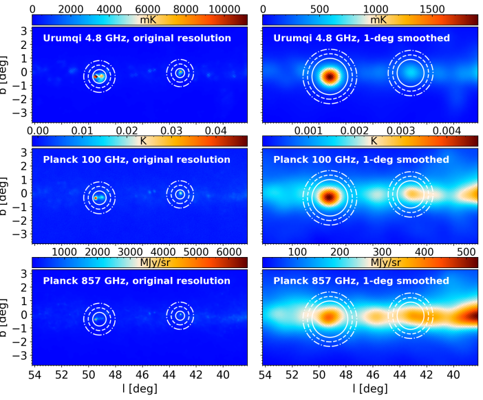
Figure 11: A comparison between the maps at their original resolution (left) and smoothed to a 1-degree beam (right) for three sample frequencies, in the area encompassing W49 and W51. The apertures employed to compute the flux densities reported in Table 13 are also shown.

References

- AMI Consortium et al. (2009) AMI Consortium et al., 2009, MNRAS, 400, 1394
- Abdo et al. (2009) Abdo A. A., et al., 2009, ApJ, 706, L1
- Ackermann et al. (2013) Ackermann M., et al., 2013, Science, 339, 807
- Ade et al. (2021) Ade P. A. R., et al., 2021, Phys. Rev. Lett., 127, 151301
- Aleksić et al. (2012) Aleksić J., et al., 2012, A&A, 541, A13
- Ali-Haïmoud (2013) Ali-Haïmoud Y., 2013, Advances in Astronomy, 2013, 462697
- Ali-Haïmoud et al. (2009) Ali-Haïmoud Y., Hirata C. M., Dickinson C., 2009, MNRAS, 395, 1055
- Ambrocio-Cruz et al. (2017) Ambrocio-Cruz P., Rosado M., de la Fuente E., Silva R., Blanco-Piñon A., 2017, MNRAS, 472, 51
- BICEP/Keck Collaboration et al. (2021) BICEP/Keck Collaboration et al., 2021, Phys. Rev. D, 103, 022004
- Battistelli et al. (2006) Battistelli E. S., Rebolo R., Rubiño-Martín J. A., Hildebrandt S. R., Watson R. A., Gutiérrez C., Hoyland R. J., 2006, ApJ, 645, L141
- Battistelli et al. (2015) Battistelli E. S., et al., 2015, ApJ, 801, 111
- Bennett et al. (2013) Bennett C. L., et al., 2013, ApJS, 208, 20
- Berkhuijsen (1972) Berkhuijsen E. M., 1972, A&AS, 5, 263
- Bik et al. (2019) Bik A., Henning T., Wu S. W., Zhang M., Brand ner W., Pasquali A., Stolte A., 2019, A&A, 624, A63
- Binder & Povich (2018) Binder B. A., Povich M. S., 2018, ApJ, 864, 136
- Bonaldi et al. (2007) Bonaldi A., Ricciardi S., Leach S., Stivoli F., Baccigalupi C., de Zotti G., 2007, MNRAS, 382, 1791
- Bonatto & Bica (2011) Bonatto C., Bica E., 2011, MNRAS, 414, 3769
- Brogan & Troland (2001) Brogan C. L., Troland T. H., 2001, ApJ, 550, 799
- Brogan et al. (2013) Brogan C. L., et al., 2013, ApJ, 771, 91
- Brun et al. (2011) Brun F., de Naurois M., Hofmann W., Carrigan S., Djannati-Ataï A., Ohm S., 2011, in Alecian G., Belkacem K., Samadi R., Valls-Gabaud D., eds, SF2A-2011: Proceedings of the Annual meeting of the French Society of Astronomy and Astrophysics. pp 545–548
- Carpenter & Sanders (1998) Carpenter J. M., Sanders D. B., 1998, AJ, 116, 1856
- Casassus et al. (2006) Casassus S., Cabrera G. F., Förster F., Pearson T. J., Readhead A. C. S., Dickinson C., 2006, ApJ, 639, 951
- Casassus et al. (2008) Casassus S., et al., 2008, MNRAS, 391, 1075
- Castelletti et al. (2011) Castelletti G., Dubner G., Clarke T., Kassim N. E., 2011, A&A, 534, A21
- Cepeda-Arroita et al. (2021) Cepeda-Arroita R., et al., 2021, MNRAS, 503, 2927
- Davies et al. (2006) Davies R. D., Dickinson C., Banday A. J., Jaffe T. R., Górski K. M., Davis R. J., 2006, MNRAS, 370, 1125
- de Oliveira-Costa et al. (1998) de Oliveira-Costa A., Tegmark M., Page L. A., Boughn S. P., 1998, ApJ, 509, L9
- de Oliveira-Costa et al. (1999) de Oliveira-Costa A., Tegmark M., Gutiérrez C. M., Jones A. W., Davies R. D., Lasenby A. N., Rebolo R., Watson R. A., 1999, ApJ, 527, L9
- De Pree et al. (2018) De Pree C. G., et al., 2018, ApJ, 863, L9
- De Pree et al. (2020) De Pree C. G., et al., 2020, AJ, 160, 234
- Demetroullas et al. (2015) Demetroullas C., et al., 2015, MNRAS, 453, 2082
- Dickinson et al. (2009) Dickinson C., et al., 2009, ApJ, 690, 1585
- Dickinson et al. (2011) Dickinson C., Peel M., Vidal M., 2011, MNRAS, 418, L35
- Dickinson et al. (2018) Dickinson C., et al., 2018, New Astron. Rev., 80, 1
- Draine (2011) Draine B. T., 2011, Physics of the Interstellar and Intergalactic Medium
- Draine & Hensley (2013) Draine B. T., Hensley B., 2013, ApJ, 765, 159
- Draine & Hensley (2016) Draine B. T., Hensley B. S., 2016, ApJ, 831, 59
- Draine & Lazarian (1998) Draine B. T., Lazarian A., 1998, ApJ, 508, 157
- Draine & Lazarian (1999) Draine B. T., Lazarian A., 1999, ApJ, 512, 740
- Dunham et al. (2010) Dunham M. K., et al., 2010, ApJ, 717, 1157
- Eden et al. (2018) Eden D. J., et al., 2018, MNRAS, 477, 3369
- Egron et al. (2016) Egron E., et al., 2016, in Supernova Remnants: An Odyssey in Space after Stellar Death. p. 18 (arXiv:1609.03882)
- Egron et al. (2017) Egron E., et al., 2017, MNRAS, 470, 1329
- Fesen (1984) Fesen R. A., 1984, ApJ, 281, 658
- Finkbeiner et al. (2002) Finkbeiner D. P., Schlegel D. J., Frank C., Heiles C., 2002, ApJ, 566, 898
- Fixsen (2009) Fixsen D. J., 2009, ApJ, 707, 916
- Galván-Madrid et al. (2013) Galván-Madrid R., et al., 2013, ApJ, 779, 121
- Gao et al. (2010) Gao X. Y., et al., 2010, A&A, 515, A64
- Gao et al. (2011) Gao X. Y., Han J. L., Reich W., Reich P., Sun X. H., Xiao L., 2011, A&A, 529, A159
- Génova-Santos et al. (2011) Génova-Santos R., Rebolo R., Rubiño-Martín J. A., López-Caraballo C. H., Hildebrandt S. R., 2011, ApJ, 743, 67
- Génova-Santos et al. (2015a) Génova-Santos R., Rubiño-Martín J. A., Rebolo R., 2015a, in Highlights of Spanish Astrophysics VIII. pp 207–212 (arXiv:1504.03514)
- Génova-Santos et al. (2015b) Génova-Santos R., Rubiño-Martín J. A., Rebolo R., 2015b, MNRAS, 452, 4169
- Génova-Santos et al. (2017) Génova-Santos R., et al., 2017, MNRAS, 464, 4107
- Génova-Santos et al. (2023) Génova-Santos R. T., Rubiño-Martín J. A., et al., 2023, MNRAS, in prep.
- Ginsburg (2017) Ginsburg A., 2017, arXiv e-prints, p. arXiv:1702.06627
- Ginsburg et al. (2015) Ginsburg A., Bally J., Battersby C., Youngblood A., Darling J., Rosolowsky E., Arce H., Lebrón Santos M. E., 2015, A&A, 573, A106
- Ginsburg et al. (2016) Ginsburg A., et al., 2016, A&A, 595, A27
- Ginsburg et al. (2017) Ginsburg A., et al., 2017, ApJ, 842, 92
- Ginsburg et al. (2020) Ginsburg A., et al., 2020, ApJS, 248, 24
- Goddi et al. (2020) Goddi C., Ginsburg A., Maud L. T., Zhang Q., Zapata L. A., 2020, ApJ, 905, 25
- González-Casanova et al. (2014) González-Casanova D. F., De Colle F., Ramirez-Ruiz E., Lopez L. A., 2014, ApJ, 781, L26
- Górski et al. (2005) Górski K. M., Hivon E., Banday A. J., Wandelt B. D., Hansen F. K., Reinecke M., Bartelmann M., 2005, ApJ, 622, 759
- Greco et al. (2018) Greco E., Miceli M., Orlando S., Peres G., Troja E., Bocchino F., 2018, A&A, 615, A157
- Green (1986) Green D. A., 1986, MNRAS, 221, 473
- Green (2014) Green D. A., 2014, Bulletin of the Astronomical Society of India, 42, 47
- Guidi et al. (2021) Guidi F., et al., 2021, MNRAS, 507, 3707
- Gwinn et al. (1992) Gwinn C. R., Moran J. M., Reid M. J., 1992, ApJ, 393, 149
- H. E. S. S. Collaboration et al. (2018) H. E. S. S. Collaboration et al., 2018, A&A, 612, A5
- Hanabata et al. (2013) Hanabata Y., Sawada M., Katagiri H., Bamba A., Fukazawa Y., 2013, PASJ, 65, 42
- Haslam et al. (1982) Haslam C. G. T., Salter C. J., Stoffel H., Wilson W. E., 1982, A&AS, 47, 1
- Hauser et al. (1998) Hauser M. G., et al., 1998, ApJ, 508, 25
- Hinshaw et al. (2013) Hinshaw G., et al., 2013, ApJS, 208, 19
- Hirayama et al. (2019) Hirayama A., Yamauchi S., Nobukawa K. K., Nobukawa M., Koyama K., 2019, PASJ, 71, 37
- Hoang & Lazarian (2016) Hoang T., Lazarian A., 2016, ApJ, 821, 91
- Hoang et al. (2010) Hoang T., Draine B. T., Lazarian A., 2010, ApJ, 715, 1462
- Hoang et al. (2013) Hoang T., Lazarian A., Martin P. G., 2013, ApJ, 779, 152
- Hoyland et al. (2012) Hoyland R. J., et al., 2012, in Millimeter, Submillimeter, and Far-Infrared Detectors and Instrumentation for Astronomy VI. p. 845233, doi:10.1117/12.925349
- Huang et al. (2020) Huang Y., Li Z., Wang W., Zhao X., 2020, MNRAS, 492, 4246
- Hwang et al. (2000) Hwang U., Petre R., Hughes J. P., 2000, ApJ, 532, 970
- Irfan et al. (2015) Irfan M. O., et al., 2015, MNRAS, 448, 3572
- Jacob et al. (2021) Jacob A. M., Menten K. M., Wiesemeyer H., Ortiz-León G. N., 2021, A&A, 650, A133
- Jonas et al. (1998) Jonas J. L., Baart E. E., Nicolson G. D., 1998, MNRAS, 297, 977
- Kamionkowski et al. (1997) Kamionkowski M., Kosowsky A., Stebbins A., 1997, Phys. Rev. D, 55, 7368
- Keohane et al. (2007) Keohane J. W., Reach W. T., Rho J., Jarrett T. H., 2007, ApJ, 654, 938
- Kogut et al. (2007) Kogut A., et al., 2007, ApJ, 665, 355
- Kokusho et al. (2013) Kokusho T., Nagayama T., Kaneda H., Ishihara D., Lee H.-G., Onaka T., 2013, ApJ, 768, L8
- Koo & Moon (1997) Koo B.-C., Moon D.-S., 1997, ApJ, 475, 194
- Koo et al. (1995) Koo B.-C., Kim K.-T., Seward F. D., 1995, ApJ, 447, 211
- Koo et al. (2005) Koo B.-C., Lee J.-J., Seward F. D., Moon D.-S., 2005, ApJ, 633, 946
- Koo et al. (2020) Koo B.-C., Kim C.-G., Park S., Ostriker E. C., 2020, ApJ, 905, 35
- Krachmalnicoff et al. (2016) Krachmalnicoff N., Baccigalupi C., Aumont J., Bersanelli M., Mennella A., 2016, A&A, 588, A65
- Kundu & Velusamy (1967) Kundu M. R., Velusamy T., 1967, Annales d’Astrophysique, 30, 59
- Kundu & Velusamy (1972) Kundu M. R., Velusamy T., 1972, A&A, 20, 237
- Kurtz et al. (1994) Kurtz S., Churchwell E., Wood D. O. S., 1994, ApJS, 91, 659
- Lazarian & Draine (2000) Lazarian A., Draine B. T., 2000, ApJ, 536, L15
- Lee et al. (2008) Lee J.-J., Koo B.-C., Yun M. S., Stanimirović S., Heiles C., Heyer M., 2008, AJ, 135, 796
- Lee et al. (2020) Lee Y.-H., Koo B.-C., Lee J.-J., 2020, AJ, 160, 263
- Leitch et al. (1997) Leitch E. M., Readhead A. C. S., Pearson T. J., Myers S. T., 1997, ApJ, 486, L23
- Lim & De Buizer (2019) Lim W., De Buizer J. M., 2019, ApJ, 873, 51
- López-Caraballo et al. (2011) López-Caraballo C. H., Rubiño-Martín J. A., Rebolo R., Génova-Santos R., 2011, ApJ, 729, 25
- Lopez et al. (2013) Lopez L. A., Ramirez-Ruiz E., Castro D., Pearson S., 2013, ApJ, 764, 50
- Loru et al. (2019) Loru S., et al., 2019, MNRAS, 482, 3857
- Lozinskaya (1981) Lozinskaya T. A., 1981, Soviet Astronomy Letters, 7, 29
- Macellari et al. (2011) Macellari N., Pierpaoli E., Dickinson C., Vaillancourt J. E., 2011, MNRAS, 418, 888
- Markwardt (2009) Markwardt C. B., 2009, in Bohlender D. A., Durand D., Dowler P., eds, Astronomical Society of the Pacific Conference Series Vol. 411, Astronomical Data Analysis Software and Systems XVIII. p. 251 (arXiv:0902.2850)
- Martin (1972) Martin A. H. M., 1972, MNRAS, 157, 31
- Mason et al. (2009) Mason B. S., Robishaw T., Heiles C., Finkbeiner D., Dickinson C., 2009, ApJ, 697, 1187
- Matsumura et al. (2017) Matsumura H., Tanaka T., Uchida H., Okon H., Tsuru T. G., 2017, ApJ, 851, 73
- Mehringer (1994) Mehringer D. M., 1994, ApJS, 91, 713
- Mezger et al. (1967) Mezger P. G., Schraml J., Terzian Y., 1967, ApJ, 150, 807
- Mitra et al. (2014) Mitra D., Green D. A., Rao A. P., 2014, in Ray A., McCray R. A., eds, IAU Symposium Vol. 296, Supernova Environmental Impacts. pp 376–377 (arXiv:1309.3078), doi:10.1017/S1743921313009903
- Moffett & Reynolds (1994) Moffett D. A., Reynolds S. P., 1994, ApJ, 437, 705
- Mufson & Liszt (1979) Mufson S. L., Liszt H. S., 1979, ApJ, 232, 451
- Murphy et al. (2010) Murphy E. J., et al., 2010, ApJ, 709, L108
- Nashimoto et al. (2020) Nashimoto M., Hattori M., Poidevin F., Génova-Santos R., 2020, ApJ, 900, L40
- Okumura et al. (2000) Okumura S.-i., Mori A., Nishihara E., Watanabe E., Yamashita T., 2000, ApJ, 543, 799
- Olbert et al. (2001) Olbert C. M., Clearfield C. R., Williams N. E., Keohane J. W., Frail D. A., 2001, ApJ, 554, L205
- Onić et al. (2012) Onić D., Urošević D., Arbutina B., Leahy D., 2012, ApJ, 756, 61
- Onić et al. (2017) Onić D., Urošević D., Leahy D., 2017, AJ, 153, 32
- Penzias et al. (1971) Penzias A. A., Jefferts K. B., Wilson R. W., 1971, ApJ, 165, 229
- Petre et al. (1988) Petre R., Szymkowiak A. E., Seward F. D., Willingale R., 1988, ApJ, 335, 215
- Planck Collaboration et al. (2011) Planck Collaboration et al., 2011, A&A, 536, A20
- Planck Collaboration et al. (2014a) Planck Collaboration et al., 2014a, A&A, 565, A103
- Planck Collaboration et al. (2014b) Planck Collaboration et al., 2014b, A&A, 571, A13
- Planck Collaboration et al. (2016a) Planck Collaboration Arnaud M., Ashdown M., Atrio-Barand ela F., Aumont J., 2016a, A&A, 586, A134
- Planck Collaboration et al. (2016b) Planck Collaboration et al., 2016b, A&A, 594, A1
- Planck Collaboration et al. (2016c) Planck Collaboration Ade P. A. R., Aghanim N., Alves M. I. R., Arnaud M., Ashdown M., Aumont J. e. a., 2016c, A&A, 594, A25
- Planck Collaboration et al. (2018) Planck Collaboration et al., 2018, A&A, 610, C1
- Planck Collaboration et al. (2020a) Planck Collaboration Aghanim N., Akrami Y., Arroja F., Ashdown M., Aumont J., Baccigalupi C. e. a., 2020a, A&A, 641, A1
- Planck Collaboration et al. (2020b) Planck Collaboration et al., 2020b, A&A, 641, A6
- Planck Collaboration et al. (2020c) Planck Collaboration et al., 2020c, A&A, 641, A11
- Planck Collaboration et al. (2020d) Planck Collaboration Aghanim N., Akrami Y., Alves M. I. R., Ashdown M., Aumont J., Baccigalupi C. e. a., 2020d, A&A, 641, A12
- Planck Collaboration et al. (2020e) Planck Collaboration Akrami Y., Andersen K. J., Ashdown M., Baccigalupi C., Ballardini M., Banday A. J. e. a., 2020e, A&A, 643, A42
- Platania et al. (2003) Platania P., Burigana C., Maino D., Caserini E., Bersanelli M., Cappellini B., Mennella A., 2003, A&A, 410, 847
- Poidevin et al. (2019) Poidevin F., et al., 2019, MNRAS, 486, 462
- Poidevin et al. (2023) Poidevin F., Génova Santos R. T., Rubiño-Martín J. A., et al., 2023, MNRAS, accepted
- Purcell et al. (2013) Purcell C. R., et al., 2013, ApJS, 205, 1
- Pye et al. (1984) Pye J. P., Becker R. H., Seward F. D., Thomas N., 1984, MNRAS, 207, 649
- Rajwade et al. (2016) Rajwade K., Seymour A., Lorimer D. R., Karastergiou A., Serylak M., McLaughlin M. A., Griessmeier J. M., 2016, MNRAS, 462, 2518
- Ranasinghe & Leahy (2018) Ranasinghe S., Leahy D. A., 2018, AJ, 155, 204
- Reich & Reich (1986) Reich P., Reich W., 1986, A&AS, 63, 205
- Reich & Reich (1988) Reich P., Reich W., 1988, A&AS, 74, 7
- Rho & Petre (1998) Rho J., Petre R., 1998, ApJ, 503, L167
- Ritchey et al. (2020) Ritchey A. M., Jenkins E. B., Federman S. R., Rice J. S., Caprioli D., Wallerstein G., 2020, ApJ, 897, 83
- Rivera-Soto et al. (2020) Rivera-Soto R., Galván-Madrid R., Ginsburg A., Kurtz S., 2020, ApJ, 899, 94
- Rivilla et al. (2016) Rivilla V. M., Fontani F., Beltrán M. T., Vasyunin A., Caselli P., Martín-Pintado J., Cesaroni R., 2016, ApJ, 826, 161
- Rivilla et al. (2017) Rivilla V. M., Beltrán M. T., Martín-Pintado J., Fontani F., Caselli P., Cesaroni R., 2017, A&A, 599, A26
- Roberts et al. (2011) Roberts H., van der Tak F. F. S., Fuller G. A., Plume R., Bayet E., 2011, A&A, 525, A107
- Rubiño-Martín et al. (2012a) Rubiño-Martín J. A., López-Caraballo C. H., Génova-Santos R., Rebolo R., 2012a, Advances in Astronomy, 2012, 351836
- Rubiño-Martín et al. (2012b) Rubiño-Martín J. A., et al., 2012b, in Ground-based and Airborne Telescopes IV. p. 84442Y, doi:10.1117/12.926581
- Rubiño-Martín et al. (2017) Rubiño-Martín J. A., et al., 2017, in Highlights on Spanish Astrophysics IX. pp 99–107
- Rubiño-Martín et al. (2023) Rubiño-Martín J. A., Guidi F., Génova Santos R. T., et al., 2023, MNRAS, accepted
- Rugel et al. (2019) Rugel M. R., et al., 2019, A&A, 622, A48
- Rybicki & Lightman (1979) Rybicki G. B., Lightman A. P., 1979, Radiative processes in astrophysics
- Sano et al. (2021) Sano H., et al., 2021, arXiv e-prints, p. arXiv:2106.12009
- Saral et al. (2017) Saral G., et al., 2017, ApJ, 839, 108
- Sato (1973) Sato F., 1973, PASJ, 25, 135
- Sato et al. (2010) Sato M., Reid M. J., Brunthaler A., Menten K. M., 2010, ApJ, 720, 1055
- Seward (1990) Seward F. D., 1990, ApJS, 73, 781
- Siegel et al. (2020) Siegel J., Dwarkadas V. V., Frank K. A., Burrows D. N., 2020, ApJ, 904, 175
- Sievers et al. (1991) Sievers A. W., Mezger P. G., Bordeon M. A., Kreysa E., Haslam C. G. T., Lemke R., 1991, A&A, 251, 231
- Silsbee et al. (2011) Silsbee K., Ali-Haïmoud Y., Hirata C. M., 2011, MNRAS, 411, 2750
- Simon et al. (2001) Simon R., Jackson J. M., Clemens D. P., Bania T. M., Heyer M. H., 2001, ApJ, 551, 747
- Stevenson (2014) Stevenson M. A., 2014, ApJ, 781, 113
- Su et al. (2014) Su Y., Fang M., Yang J., Zhou P., Chen Y., 2014, ApJ, 788, 122
- Sun et al. (2011) Sun X. H., Reich W., Han J. L., Reich P., Wielebinski R., Wang C., Müller P., 2011, A&A, 527, A74
- Tavani et al. (2010) Tavani M., et al., 2010, ApJ, 710, L151
- Tian & Leahy (2013) Tian W. W., Leahy D. A., 2013, ApJ, 769, L17
- Tibbs et al. (2010) Tibbs C. T., et al., 2010, MNRAS, 402, 1969
- Torres et al. (2003) Torres D. F., Romero G. E., Dame T. M., Combi J. A., Butt Y. M., 2003, Phys. Rep., 382, 303
- Trujillo-Bueno et al. (2002) Trujillo-Bueno J., Moreno-Insertis F., Sánchez F., eds, 2002, Astrophysical spectropolarimetry
- Ustamujic et al. (2021) Ustamujic S., Orlando S., Greco E., Miceli M., Bocchino F., Tutone A., Peres G., 2021, A&A, 649, A14
- Vaillancourt (2006) Vaillancourt J. E., 2006, PASP, 118, 1340
- Vastel et al. (2017) Vastel C., Mookerjea B., Pety J., Gerin M., 2017, A&A, 597, A45
- Vidal et al. (2011) Vidal M., et al., 2011, MNRAS, 414, 2424
- Vidal et al. (2015) Vidal M., Dickinson C., Davies R. D., Leahy J. P., 2015, MNRAS, 452, 656
- Vidal et al. (2020) Vidal M., Dickinson C., Harper S. E., Casassus S., Witt A. N., 2020, MNRAS, 495, 1122
- Watanabe et al. (2017) Watanabe Y., Nishimura Y., Harada N., Sakai N., Shimonishi T., Aikawa Y., Kawamura A., Yamamoto S., 2017, ApJ, 845, 116
- Watson et al. (2005) Watson R. A., Rebolo R., Rubiño-Martín J. A., Hildebrandt S., Gutiérrez C. M., Fernández-Cerezo S., Hoyland R. J., Battistelli E. S., 2005, ApJ, 624, L89
- Watts et al. (2015) Watts D. J., et al., 2015, ApJ, 814, 103
- Westerhout (1958) Westerhout G., 1958, Bulletin of the Astronomical Institutes of the Netherlands, 14, 215
- Wilson et al. (1970) Wilson T. L., Mezger P. G., Gardner F. F., Milne D. K., 1970, Astrophysical Letters, 5, 99
- Wilson et al. (2009) Wilson T. L., Rohlfs K., Hüttemeister S., 2009, Tools of Radio Astronomy, doi:10.1007/978-3-540-85122-6.
- Wolleben et al. (2006) Wolleben M., Landecker T. L., Reich W., Wielebinski R., 2006, A&A, 448, 411
- Wu et al. (2016) Wu S.-W., Bik A., Bestenlehner J. M., Henning T., Pasquali A., Brandner W., Stolte A., 2016, A&A, 589, A16
- Xu et al. (2009) Xu Y., Reid M. J., Menten K. M., Brunthaler A., Zheng X. W., Moscadelli L., 2009, ApJ, 693, 413
- Yoshiike et al. (2017) Yoshiike S., Fukuda T., Sano H., Fukui Y., 2017, in 6th International Symposium on High Energy Gamma-Ray Astronomy. p. 040039, doi:10.1063/1.4968943
- Ysard & Verstraete (2010) Ysard N., Verstraete L., 2010, A&A, 509, A12
- Zaldarriaga & Seljak (1997) Zaldarriaga M., Seljak U., 1997, Phys. Rev. D, 55, 1830
- Zhang et al. (2013) Zhang B., Reid M. J., Menten K. M., Zheng X. W., Brunthaler A., Dame T. M., Xu Y., 2013, ApJ, 775, 79
- Zhang et al. (2017) Zhang M. F., Tian W. W., Leahy D. A., Zhu H., Cui X. H., Shan S. S., 2017, ApJ, 849, 147
- Zhang et al. (2018) Zhang S., et al., 2018, ApJ, 859, 141
- Zhou et al. (2011) Zhou X., Miceli M., Bocchino F., Orland o S., Chen Y., 2011, MNRAS, 415, 244
- Zhu et al. (2014) Zhu H., Tian W. W., Zuo P., 2014, ApJ, 793, 95