Local consistency as a reduction between constraint satisfaction problems

Abstract.

We study the use of local consistency methods as reductions between constraint satisfaction problems (CSPs), and promise version thereof, with the aim to classify these reductions in a similar way as the algebraic approach classifies gadget reductions between CSPs. This research is motivated by the requirement of more expressive reductions in the scope of promise CSPs. While gadget reductions are enough to provide all necessary hardness in the scope of (finite domain) non-promise CSP, in promise CSPs a wider class of reductions needs to be used.

We provide a general framework of reductions, which we call consistency reductions, that covers most (if not all) reductions recently used for proving NP-hardness of promise CSPs. We prove some basic properties of these reductions, and provide the first steps towards understanding the power of consistency reductions by characterizing a fragment associated to arc-consistency in terms of polymorphisms of the template. In addition to showing hardness, consistency reductions can also be used to provide feasible algorithms by reducing to a fixed tractable (promise) CSP, for example, to solving systems of affine equations. In this direction, among other results, we describe the well-known Sherali-Adams hierarchy for CSP in terms of a consistency reduction to linear programming.

1. Introduction

Is it possible to find a mathematical invariant that characterises when one computational problem reduces to another by a polynomial-time (Karp) reduction? This question is far beyond our current understanding as it would imply a characterisation of polynomial-time solvable problems, possibly resolving the P vs. NP problem. The present paper is a contribution to the effort to provide a partial answer to this question by characterising certain well-structured efficient reductions between structured problems.

Though it is usually not described in these words, a characterisation of a subclass of polynomial-time (in fact log-space) reductions in terms of certain mathematical invariants of the problem is the core of a theory referred to as the algebraic approach to the constraint satisfaction problem. Development of this theory started with Jeavons, Cohen, and Gyssens [32] and Bulatov, Jeavons, and Krokhin [16]. The scope of this theory is the constraint satisfaction problem (CSP) which is a decision problem whose input consists of a list of variables, with each variable allowed to attain values from a finite domain, and a list of constraints each involving a tuple of variables. The goal is to decide if there is an assignment of values to variables that simultaneously satisfies all the constraints. By restricting the shape of the constraints allowed in a CSP one can encode a large family of computational problems, including SAT, graph $k$-colouring, or solving systems of linear equations. Many of these problems naturally arise in various settings. These CSPs possess great expressiveness power and, as proven by Feder and Vardi [26], finite-domain CSPs is one of the largest natural subclasses of NP, defined via syntactic prescriptions, that could exhibit a P vs. NP-complete dichotomy. Furthermore, CSPs are well-structured from a mathematical perspective since every CSP is parametrised by a single relational structure. Consequently, significant efforts have been devoted to classifying their computational complexity via the above mentioned algebraic approach, culminating with a celebrated dichotomy theorem of Bulatov [17] and Zhuk [48].

The essence of the algebraic approach is a characterisation of gadget reductions between constraint satisfaction problems in terms of invariants of the problem called polymorphisms. Loosely speaking, a gadget reduction replaces each variable of the input with a tuple of variables of a fixed length, and each constraint on the input with a gadget of constraints on the newly introduced variables (possibly introducing more new variables). A remarkable fact is that, in the realm of finite template CSPs, gadget reductions are enough to provide all necessary NP-hardness, i.e., a finite template CSP is NP-complete if all other finite template CSPs reduce to it via a gadget reduction, and in P otherwise. The tractability side of the CSP dichotomy is given by providing an efficient algorithm for solving all other CSPs. The algorithms of Bulatov [17] and Zhuk [48] were the last piece of the dichotomy to be proven, and both of them rely on a deep understanding of structural properties of CSP templates.

A recent popular direction of CSP research is focused on a more general version of CSPs, promise constraint satisfaction problems. In this promise version of the problem, each instance comes with two versions of each constraint, a stronger and a weaker one. The goal is then decide between two (disjoint, but not complementary) cases: all stronger constraints can be satisfied, or not even the weaker constraints can be satisfied. A prominent problem described in this scope is approximate graph colouring which asks, e.g., to decide between graphs that are 3-colourable and those that are not even 6-colourable. A systematic study of promise CSPs has been started by Austrin, Guruswami, and Håstad [4] which studied a certain promise version of SAT, and continued in a series of papers including generalisations of the algebraic approach to promise CSPs by Brakensiek and Guruswami [13] and Barto, Bulín, Krokhin, and Opršal [6].

While the extension of the algebraic approach for promise CPS has proven fruitful. There is a solid basis for an argument that any theory aiming to tackle a full classification of promise CSPs must incorporate a richer notion of reduction as, unlike in (classic) CSP, gadget reductions alone cannot adequately explain many of the existing NP-hardness results, e.g., those by Dinur, Regev, and Smyth [24]; Huang [31]; Austrin, Guruswami, and Håstad [4]; Krokhin and Opršal [36]; Ficak, Kozik, Olšák, and Stankiewicz [27]; Wrochna and Živný [47]; Brandts, Wrochna, and Živný [15]; Barto, Battistelli, and Berg [5]; Nakajima and Živný [40]. These hardness results usually rely on variations of the PCP theorem of Arora and Safra [2] which is better suited for a different, more analytical, approximation version of CSPs. Indeed, new reductions for promise CSPs have been called for in Barto, Bulín, Krokhin, and Opršal [6] and Barto and Kozik [9].

The primary objective of the present paper is to offer a novel perspective on the complexity landscape of CSPs and promise CSPs that is focused on reductions rather than algorithms, or algebraic hardness conditions. We aim to identify a class of efficient reductions that can potentially fulfil a similar role to that of gadget reductions in a broader framework of (promise) CSPs. To this end, the suggested class of reductions should have the following properties:

• robustness, informally meaning that the notion of reduction remains invariant under minor variations in its definition. In particular, it should be closed under composition. In the scope of (promise) CSPs, it is also natural to require that the reductions are monotone with respect to the homomorphism order, so that the structure of the problem is preserved.

• expressiveness, that is, it should significantly extend the capabilities of gadget reductions.

• characterisability, meaning that it must be possible to characterise, in some terms similar to the algebraic characterisation of gadget reductions, whether a given (promise) CSP reduces to another given (promise) CSP.

Our contributions

We introduce a new general class of reductions between (promise) CSPs, referred to as $k$-consistent reductions or Datalog^∪ reductions, and supplement it with a series of results that showcase the robustness and expressiveness of this family of reductions. Furthermore, we take initial steps towards its characterisability. A fully fledged theory for $k$-consistency reductions would have several overreaching consequences and, hence, it falls beyond the scope of the present paper, which aims solely to initiate it.

Robustness

We provide two alternative equivalent definitions of this class of reductions:

First, we describe our suggested class of reductions in the language of logic of Datalog programs endowed with a new operator that allows to take disjoint union of relations. These reductions, referred to as Datalog^∪ reductions, are loosely described as monotone logical interpretations in the logic of Datalog with disjoint unions.

Second, in a combinatorial language. We express the reductions as a combination of the local consistency algorithm for (promise) CSPs and gadget reductions. This construction depends, apart from the templates of the two (promise) CSPs involved, on a single parameter $k$. This motivates the choice of the terminology $k$-consistency reduction.

The three following theorems, stated in Section 3, constitute the core of the robustness of our class of reductions:

• We prove that every gadget reduction is expressible equivalently as a Datalog^∪ reduction (Theorem 3.12). This is an analogue of Theorem 5 of Atserias, Bulatov, and Dawar [3], which establishes that if a CSP is reducible to another CSP by a gadget reduction, it can also be reduced by a Datalog interpretation with parameters. Unlike the result of [3], our result applies in the promise setting.

• We show that the two above formalisms have the same power when used as reductions between promise CSPs (Theorem 3.18 and Corollary 3.19). Besides providing further evidence on the robustness of our reduction, this result has the following practical by-product: it allows to move freely between the two formalisms whenever one of them is more suitable for a given proof (e.g., our third theorem below). The proof of Theorem 3.18 is based on the well-known equivalence of local consistency checking and Datalog for solving CSPs. However, since now gadget reductions are an inherent part of $k$-consistency reductions, it is additionally necessary to understand how Datalog interacts with gadget reductions, and the proof uncovers an interesting interplay between Datalog and the algebraic theory of gadget reductions.

• Further, we show that Datalog^∪ reductions compose (Theorem 3.13). This theorem is relatively straightforward to prove in the logic formalism, and together with the previous theorem shows that $k$-consistency reductions compose (though the parameter $k$ does not need to remain constant). The latter has a few practical implications. It is worth mentioning that a weaker variant of $k$-consistency reductions, introduced by Barto and Kozik [9] to provide a simpler proof of some consequences of the PCP theorem in the promise CSP setting, does not compose.

Expressiveness

We provide a few examples to illustrate the power of $k$-consistency reductions.

First, note that it is consistent with the current understanding of complexity of promise CSPs that a promise CSP is NP-hard if and only if it allows a $k$-consistency reduction from an NP-hard CSP (e.g., graph 3-colouring). For example, the reductions of Barto and Kozik [9] are covered by $k$-consistency reductions, and consequently many results about NP-hardness of promise CSPs can be explained by a $k$-consistency reduction including the hardness of $5$ colouring $3$-colourable graphs [6] and the NP-hardness in [24; 4; 36; 27; 5; 40]. The NP-hardness of colouring $k$-colourable graphs with $\binom{k}{\lfloor k/2\rfloor}-1$ colours provided by Wrochna and Živný [47] (which is the current state-of-the-art for $k\geq 5$) is also obtained by a $k$-consistency reduction from a previous result of Huang [31].

Second, several well-known hierarchies of relaxation algorithms for promise CSPs fall within our framework. A comprehensive look at hierarchies is given in Section 4 where we describe several hierarchies in terms of $k$-consistency reductions to a fixed problem. This includes the bounded width hierarchy (i.e., the hierarchy of promise CSPs expressible by Datalog), and the Sherali-Adams hierarchy of linear programming for promise CSPs. Furthermore, we show that the Sherali-Adams hierarchy of (promise) CSPs coincides with the hierarchy of (promise) CSPs reducible to linear programming by a $k$-consistency reduction (Theorem 4.5). A different framework to study hierarchies of relaxations of algorithms was recently introduced by Ciardo and Živný [22]. The Ciardo-Živný hierarchy is always subsumed by the hierarchy of $k$-consistency reductions to a fixed problem, and in some cases, e.g., the Sherali-Adams hierarchy, both hierarchies align perfectly.

One of the new hierarchies is of particular interest to us — the hierarchy of problems that reduce via a $k$-consistency reduction to solving linear equations with integer coefficients. We provide several pieces of evidence for our belief that this hierarchy of relaxations might solve all finite-template CSPs solvable by algorithms of Bulatov [17] and Zhuk [48]. If true, this would yield a substantially simpler polynomial-time algorithm for such CSPs, and a new proof of the CSP dichotomy.

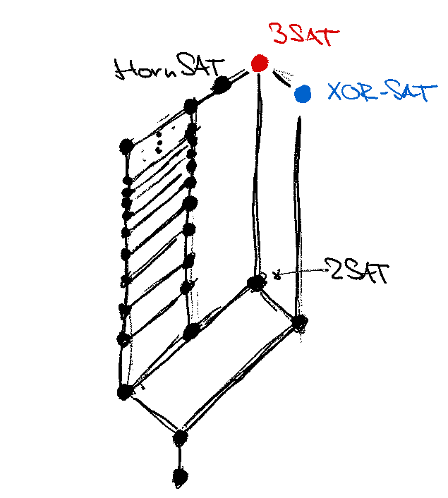
(a) gadget

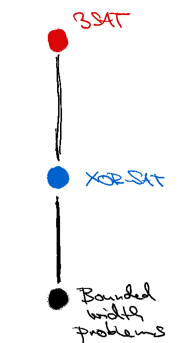
(b) Datalog^∪

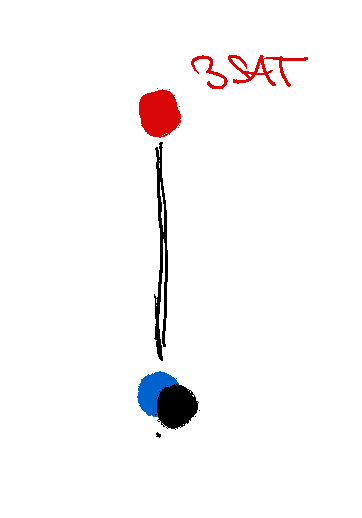
(c) polynomial-time

Figure 1. Boolean CSPs ordered by three classes of reductions with examples of problems belonging to some classes.

As a final example of the enhanced power of $k$-consistency reductions, see Figure 1 which shows all Boolean CSPs ordered by three types of reductions (Fig. 1(a) is due to Bodirsky and Vucaj [12]), and confirms our conjecture in the Boolean case.

Since consistency reductions contain, as a particular case, gadget reductions, it follows that any class of (promise) CSPs closed under consistency reductions can be, at least theoretically, described in terms of polymorphisms. This is a very desirable feature as polymorphisms lie at the heart of the algebraic approach. As a direct consequence of our findings it follows that both the class of promise CSPs solvable by local consistency and the class of promise CSPs solvable by some level of the Sherali-Adams relaxation are closed under gadget reductions. While the former result had previously been established in [6, Lemma 7.5] extending an analogous result for non-promise CSPs by Larose and Zádori [39], the latter result, in its full generality, is new. Prior to our work it had only been known for the particular case of non-promise CSPs where it can be derived by combining the results of Thapper and Živný [44] and Barto and Kozik [8].

Characterisability

As further evidence of a possible characterisability of Datalog^∪ reductions we describe a characterisation of a special case of $k$-consistency reduction, referred to as arc-consistency reduction (which is obtained by replacing enforcing $k$-consistency in the $k$-consistency reduction with the enforcing arc-consistency instead), in terms of a certain transformation of polymorphisms of the templates (see Theorem 5.11).

We present all results and proofs in a multisorted promise setting to provide wide applicability. The multisorted framework does not increase the complexity of the proofs, merely the complexity of notation. Moreover, as noted in [9, Section B.4], it provides a natural setting for the theory since it places (layered) label cover problem, whose promise version is used as an intermediate step in reductions (both in this paper and in the algebraic characterisation of gadget reductions [6, Theorem 3.12]), into the framework of CSPs. In addition, several of the key concepts introduced here (e.g., the extension of Datalog with disjoint unions) are more naturally expressed in the multisorted setting.

Organisation of the paper

We present basic definitions and notation in Section 2. This is followed by the definition of our framework and formulation of the basic theorems of our theory in Section 3. Section 4 describes several hierarchies in terms of $k$-consistency reductions, and discusses evidence for our conjecture about tractability of finite-template CSPs. In Section 5, we describe the characterisation of the arc-consistency reduction. And finally, in Section 6, we outline a few directions for future research, and possible applications of the theory developed in the present paper.

The appendices contain detailed proofs of claims made in the main part of the paper, further results, and several examples establishing wider context of consistency reductions. We present appendices in slightly different order from the sections of the main part to account for interdependencies. Appendices A, B, and C contain extended materials for Sections 3, 5, and 4, respectively.

2. Preliminaries

Many of constructions described in this paper can be defined using several different languages, e.g., an instance of a CSP can be viewed as a list of constraints, a logical formula, or a relational structure. In this paper, the structural perspective takes precedence.

Sets are generally denoted by capital letters, and integers by lower-case letters. We often do not explicitly specify that such symbols represent sets, or integers when it is clear from the context, e.g., when the symbol appears in an index.

We denote by $[n]$ the set of the first $n$ positive integers, i.e., $[n]=\{1,\dots,n\}$. We denote the set of all functions $f\colon X\to A$ by $A^{X}$, and for such a function $f$ and $Y\subseteq X$, we denote its restriction to $Y$ by $f|_{Y}\colon Y\to A$. For a function $\pi\colon X\to Y$ and $y\in Y$, we denote by $\pi^{-1}(y)$ the set of preimages of $y$ under $\pi$, i.e., the set $\{x\in X\mid\pi(x)=y\}$. We will denote entries in a tuple $a$ by lower indices, i.e., $a=(a_{1},\dots,a_{k})$, and occasionally view a tuple $a\in A^{k}$ as a function $a\colon[k]\to A$, and hence $a(i)$ is an alternative notation for $a_{i}$. Finally, we will write $f\circ g$ for the composition of $f$ and $g$ and $fg(x)$ for $(f\circ g)(x)$. We denote the identity mapping on a set $X$ by $1_{X}$.

2.1. Constraint satisfaction problems

To settle on the playing field, we formally define the constraint satisfaction problem, and its promise variant. We refer to Barto, Krokhin, and Willard [10] for a deeper exposition of the algebraic theory of CSPs, and to Krokhin and Opršal [37] for more background and examples of promise CSPs. We start with a definition of the uniform CSP, which we give to provide intuition for typed fixed-template CSPs. Further, throughout the paper will will exclusively work with a fixed-template CSP formulated as a homomorphism problem which we define below.

Definition 2.1.

The constraint satisfaction problem gets on input a list of variables with each variable $v$ assigned a finite domain $D_{v}$, and a list of constraints each of the form $(v_{1},\dots,v_{k})\in R$ where $R\subseteq D_{v_{1}}\times\dots\times D_{v_{k}}$ is given as a list of tuples (the number $k$ is called the arity of the constraint and the tuple $(v_{1},\dots,v_{k})$ is called the scope of the constraint). The goal is to decide if there is an assignment $s$ with $s(v)\in D_{v}$ for each variable $v$ that simultaneously satisfies all of the constraints, i.e., $(s(v_{1}),\dots,s(v_{k}))\in R$ for each constraint as above.

Commonly, instances are restricted in some way, e.g., we could insist that all constraints are of arity at most $m$ (i.e., $k\leq m$ in the definition above) for a fixed $m$ to get $m$-CSP. A 2-CSP where each constraint is a graph of a function, i.e., of the form $\pi(v_{1})=v_{2}$ for some $\pi\colon D_{v_{1}}\to D_{v_{2}}$ is called label cover. Another reasonable restriction is to limit the domains; we could fix a set $D$ and require that $D_{v}=D$ for each variable $v$ to get the more usual single-sorted definition of the CSP.

Let us move to the fixed-template CSP which we define as a homomorphism problem for typed (or multi-sorted) structures.

Definition 2.2.

A (finite) typed signature $\Sigma$ has two parts: (1) a finite set, the elements of which are called $\Sigma$-types and (2) a finite set of relation symbols, called $\Sigma$-symbols. Every $\Sigma$-symbol $R$ has associated an arity tuple $(t_{1},\dots,t_{k})$ of $\Sigma$-types, denoted by $ar_{R}$. The number $k$ is called the arity of $R$.

A typed relational structure of signature $\Sigma$ (or simply, a $\Sigma$-structure) $\mathbf{A}$ is an object with the following ingredients: a set $A_{t}$ for each $\Sigma$-type $t$, and a relation $R^{\mathbf{A}}\subseteq A_{t_{1}}\times\dots\times A_{t_{k}}$ for each $\Sigma$-symbol where $(t_{1},\dots,t_{k})=\operatorname{ar}_{R}$.

Such a structure $\mathbf{A}$ is said to be finite if all $A_{t}$’s are finite. Note that we denote the domains of some structure by the same letter, e.g., a structure $\mathbf{X}$ has domains $X_{t},X_{s},\dots$ where $t,s,\dots$ are types, and if the signature of $\mathbf{X}$ has only one type, we denote its domain simply by $X$.

One way to think about such structures is imagine them as a single-sorted structure whose domain is the disjoint union of the domains $A_{t}$, and each element has a given type (types can be also viewed as colours — having in mind that each element is coloured with exactly one colour). The relations then only relate elements of given types. In concordance with this interpretation we will call any $a\in A_{t}$ an element of $\mathbf{A}$ of type $t$. We do not consider two elements of $\mathbf{A}$ to be equal unless they have the same type. For example, if $\mathbf{A}$ has two domains $A_{t}=A_{s}=\{0,1\}$, we will view it as a structure with four elements. We will also use the symbol $A$ for the disjoint union of all $A_{t}$’s, and often write $x\in\mathbf{A}$ instead of $x\in A$. Throughout this paper we will often say structure instead of typed relational structure. We will usually not specify the signature explicitly, and assume that, e.g., if $\phi$ is a transformation on structures of certain signature, and $\mathbf{A}$ is a structure to which $\phi$ is applied, then the signature of $\mathbf{A}$ agrees with the signature required on the input. We will sometimes write a structure $\mathbf{A}$ as a tuple $(A_{t},A_{s},\dots;R^{\mathbf{A}},S^{\mathbf{A}},\dots)$; first listing its domains for all types $t,s,\dots$, and then listing its relations for all symbols $R,S,\dots$. When we use this notation the order is fixed for each signature $\Sigma$.

Loosely speaking, a homomorphism between two structures of the same signature is a mapping that maps elements of one structure to elements of the second structure that preserves types and all relations. Formally, we define a homomorphism as follows.

Definition 2.3.

Given two structures $\mathbf{A}$ and $\mathbf{B}$ of the same signature, a homomorphism from $\mathbf{A}$ to $\mathbf{B}$ is a collection of maps $f_{t}\colon A_{t}\to B_{t}$, one for each type $t$, such that for each relational symbol $R$ and $(a_{1},\dots,a_{k})\in R^{\mathbf{A}}$, we have

$$(f_{\operatorname{ar}_{R}(1)}(a_{1}),\dots,f_{\operatorname{ar}_{R}(k)}(a_{k}))\in R^{\mathbf{B}}.$$

Below, we will simply write $f(a)$ instead of $f_{t}(a)$ if $f$ is a collection of mappings as above, and the type $t$ of $a$ is clear from the context. We write $f\colon\mathbf{A}\to\mathbf{B}$ if $f$ is a homomorphism, and $\mathbf{A}\to\mathbf{B}$ if such a homomorphism exists (in particular, $\mathbf{A}$ and $\mathbf{B}$ have the same signature).

We say that two structures $\mathbf{A}$ and $\mathbf{B}$ are isomorphic if there are homomorphisms $f\colon\mathbf{A}\to\mathbf{B}$ and $g\colon\mathbf{B}\to\mathbf{A}$ such that $fg(b)=b$ for all $b\in B$ and $gf(a)=a$ for all $a\in A$.

Having settled on these definitions, we are ready to define a fixed-template CSP and its promise variant.

Definition 2.4.

Let $\mathbf{A}$ be a $\Sigma$-structure. The (typed) constraint satisfaction problem with template $\mathbf{A}$ is a decision problem whose goal is: given a $\Sigma$-structure $\mathbf{X}$, decide whether $\mathbf{X}\to\mathbf{A}$. We denote this problem by $\operatorname{CSP}(\mathbf{A})$.

Definition 2.5.

Let $\mathbf{A}$ and $\mathbf{A}^{\prime}$ be two $\Sigma$-structures such that $\mathbf{A}\to\mathbf{A}^{\prime}$. We define the (typed) promise constraint satisfaction problem with template $(\mathbf{A},\mathbf{A}^{\prime})$ as a promise problem whose goal is, on an input $\mathbf{X}$ which is a $\Sigma$-structure, to output yes if $\mathbf{X}\to\mathbf{A}$, and no if $\mathbf{X}\not\to\mathbf{A}^{\prime}$. We denote this problem by $\operatorname{PCSP}(\mathbf{A},\mathbf{A}^{\prime})$,

A pair of structures $\mathbf{A}$, $\mathbf{A}^{\prime}$ with $\mathbf{A}\to\mathbf{A}^{\prime}$ is called a promise template. We assume that $\mathbf{A}$ in a promise template is finite unless explicitly specified otherwise.

Note that in the promise version, the requirement that $\mathbf{A}\to\mathbf{A}^{\prime}$ ensures that the yes- and no-instances are disjoint. Alternatively, one could define a promise CSP as a promise search problem where the goal would be, given $\mathbf{X}$ that is promised to map to $\mathbf{A}$ via a homomorphism, to find a homomorphism $\mathbf{X}\to\mathbf{A}^{\prime}$. It is currently not known whether these two versions of promise CSPs are of equivalent complexity. This paper focuses on the decision version of promise CSP though a few results (mostly with some caveats) apply also to the search version. Finally, note that $\operatorname{CSP}(\mathbf{A})$ is $\operatorname{PCSP}(\mathbf{A},\mathbf{A})$, and therefore every result about promise CSPs is applicable to CSPs.

Every instance $\mathbf{X}$ of $\operatorname{CSP}(\mathbf{A})$, i.e., a structure $\mathbf{X}$ of the same signature as $\mathbf{A}$, can be interpreted as an instance of the uniform CSP in the following way: the variables are elements of $\mathbf{X}$, where each variable $v\in X_{t}$ is assigned the domain $A_{t}$, and constraints are of the form $(v_{1},\dots,v_{k})\in S$ where $(v_{1},\dots,v_{k})$ is a tuple in $R^{\mathbf{X}}$ and $S=R^{\mathbf{A}}$. We also note that every instance of the uniform CSP can be decoded into a pair $(\mathbf{X},\mathbf{A})$ of structures of the same signature, so that the instance is solvable if and only if $\mathbf{X}\to\mathbf{A}$. In the rest of the paper, we will only work with fixed-template CSPs, though we borrow the following terminology from the uniform CSP: A constraint of an instance $\mathbf{X}$ of $\operatorname{PCSP}(\mathbf{A},\mathbf{A}^{\prime})$ is an expression of the form $(v_{1},\dots,v_{k})\in R^{\mathbf{X}}$ which we formally view as a pair $((v_{1},\dots,v_{k}),R)$ where $v_{1},\dots,v_{k}$ are elements of $X$ and $R$ is a relational symbol such that the expression is satisfied. The tuple $(v_{1},\dots,v_{k})$ is called the scope of the constraint.

Let us finish this subsection with the definition of a power of a structure which is a standard construction that we will use on several occasions throughout the paper. We define powers with arbitrary sets as exponents.

Definition 2.6.

Let $X$ be a set, and $\mathbf{B}=(B_{t},B_{s},\dots;R^{\mathbf{B}},S^{\mathbf{B}},\dots)$ be a $\Sigma$-structure. The $X$-fold direct power of $\mathbf{B}$ is the $\Sigma$-structure

$$\mathbf{B}^{X}=(B_{t}^{X},B_{s}^{X},\dots;R^{\mathbf{B}^{X}},S^{\mathbf{B}^{X}},\dots),$$

where $B_{t}^{X}=(B_{t})^{X}$ and, for each $\Sigma$-symbol $R$, $R^{\mathbf{B}^{X}}$ contains all tuples $(b_{1},\dots,b_{k})$ of functions $b_{i}\colon X\to B_{\operatorname{ar}_{R}(i)}$, such that $(b_{1}(x),\dots,b_{k}(x))\in R^{\mathbf{B}}$ for all $x\in X$.

2.2. Label cover

The label cover problem mentioned above will play a key role in this paper, since many reductions will be either implicitly, or explicitly reductions between variants of label cover and other CSPs. Recall that the label cover is a binary CSP where each constraint is of the form $\pi(u)=v$ for some mapping $\pi\colon D_{u}\to D_{v}$. We can view this problem as a fixed-template CSP using the multi-sorted approach although we have to allow an infinite signature.

Definition 2.7.

(Label cover problem) The signature of label cover has a type $X$ for each finite set $X$. Further, for each pair of finite sets $X$, $Y$, and every mapping $\pi\colon X\to Y$ it has a relation symbol $E_{\pi}$ with arity tuple $(X,Y)$.

The label cover problem is $\operatorname{CSP}(\mathbf{P})$ where its template $\mathbf{P}$ is the structure with $P_{X}=X$ for each finite set $X$ and $E_{\pi}^{\mathbf{P}}=\{(x,\pi(x))\mid x\in X\}$ for each $\pi\colon X\to Y$.

We refine the definition of finite structure to account for infinite signatures, and encoding of a label cover instance in a finite amount of space. We say that a structure $\mathbf{D}$ in the above signature is finite if $D_{X}$ is non-empty and finite for finitely many types $X$, and empty for all other types. Note that this condition implies that $E_{\pi}^{\mathbf{D}}\neq\emptyset$ for finitely many relational symbols $E_{\pi}$. Such a structure can be then encoded as a finite list of all its elements and a finite list of all its non-empty relations. We will call such structures label cover instances.

We say that a signature $\Sigma$ is a finite reduct of the label cover signature if the types of $\Sigma$ consist of a finite list of label cover types, i.e., a finite list of sets, and relations of $\Sigma$ consist of finitely many relational symbols of label cover. We say that a $\Sigma$-structure $\mathbf{A}$ is a $\Sigma$-reduct of $\mathbf{B}$ if $A_{X}=B_{X}$ for each $\Sigma$-type $X$, and $E_{\pi}^{\mathbf{A}}=E_{\pi}^{\mathbf{B}}$ for each $\Sigma$-relation $E_{\pi}$.

Finally, let us mention that a promise version of (a reduct of) the label cover problem (denoted by $\operatorname{PMC}_{\mathscr{M}}$) was used to provide the generalisation of the algebraic approach to promise CSP, see [6, Definition 3.10 & Theorem 3.12]. We will also use similarly defined promise versions of label cover in the present paper, but postpone the definition until Appendix B.1.

2.3. Reductions

We formally define a notion of a reduction between two (promise) CSPs. A reduction between decision problems is a (usually efficiently computable) function that maps instances of one problem to instances of the other problem in such a way that the answer is preserved.

Definition 2.8.

Let $\mathbf{A},\mathbf{A}^{\prime}$ and $\mathbf{B},\mathbf{B}^{\prime}$ be two promise templates. We say that a mapping $\psi$ is a reduction from $\operatorname{PCSP}(\mathbf{A},\mathbf{A}^{\prime})$ to $\operatorname{PCSP}(\mathbf{B},\mathbf{B}^{\prime})$ if it maps structures $\mathbf{X}$ with the same signature as $\mathbf{A}$ to structures with the same signature as $\mathbf{B}$, in such a way that: (1) if $\mathbf{X}\to\mathbf{A}$ then $\psi(\mathbf{X})\to\mathbf{B}$, and (2) if $\mathbf{X}\not\to\mathbf{A}^{\prime}$ then $\psi(\mathbf{X})\not\to\mathbf{B}^{\prime}$.

The first item, preserving the yes instances, is usually referred to as completeness, and the second, preserving the no instances, as soundness. We will usually use and prove the soundness in its converse form: if $\psi(\mathbf{X})\to\mathbf{B}^{\prime}$ then $\mathbf{X}\to\mathbf{A}^{\prime}$. Note that, in the case of a reduction between the search version of (promise) CSPs, it would be necessary to additionally require that this converse is witnessed by an efficiently computable function that, given a homomorphism $\psi(\mathbf{X})\to\mathbf{B}^{\prime}$, outputs a homomorphism $\mathbf{X}\to\mathbf{A}^{\prime}$.

Reductions are more general than algorithms: every decision algorithm can be viewed as a reduction to a problem with two admissible instances yes and no where yes is the positive instance. In our setting, we use a specific CSP instead of this trivial problem, so that our reductions do not leave the scope of (promise) CSPs. The template of this ‘trivial CSP’ is a structure in a very degenerate signature which allows only two structures.

Definition 2.9.

Let $\Omega$ be a signature with no types and one nullary relational symbol $C$. We define $\bot$ as the structure where $C^{\bot}$ is the empty nullary relation. The trivial CSP is the CSP with template $\bot$.

There are only two $\Omega$-structures: $\bot$ and $\top$. The structure $\bot$ is defined above and $\top$ is the structure with the non-empty nullary relation. Note that $\bot\to\bot$ and $\top\not\to\bot$, hence $\bot$ is a positive instance and $\top$ is a negative instance of $\operatorname{CSP}(\bot)$.

We will also implicitly assume that all (promise) CSPs considered in this paper have negative instances — this can be always ensured by adding a nullary constraint that cannot be satisfied.

3. Local consistency reductions

We will define several classes of efficiently computable functions on relational structures: gadget reductions, Datalog interpretations, and (local) consistency reductions. Also, we will show that arbitrary composition of Datalog interpretations and gadget replacements are equivalent to consistency reductions in the sense that one reduction can be used in the place of the other when reducing between two (promise) CSPs; this statement is formalised in Corollary 3.19 below. While Datalog interpretations and gadgets have many parameters that could be adjusted, consistency has only one parameter, a width $k$, in this sense we can view local consistency as a canonical normal form of these reductions.

3.1. Gadget reductions

Gadget reductions are the more traditional reductions in the realm of finite-template CSPs and promise CSPs. They have been classified by the algebraic approach. We outline this classification briefly in Section 5 below, and refer to Barto, Bulín, Krokhin, and Opršal [6], Barto, Krokhin, and Willard [10], or Krokhin and Opršal [37] for a detailed exposition.

Note that, customarily, the algebraic approach focuses on the templates. That is, it aims to explore under which conditions on $\mathbf{A}$ and $\mathbf{B}$ there exists a gadget reduction from $\operatorname{CSP}(\mathbf{B})$ to $\operatorname{CSP}(\mathbf{A})$. This relationship between $\mathbf{A}$ and $\mathbf{B}$ is explained using pp-interpretations (which are a special case of Datalog interpretations that we define below). However, in the present paper, our focus shifts to understanding what the reduction does to an instance $\mathbf{X}$ of $\operatorname{CSP}(\mathbf{B})$? We start with giving a formal definition of a gadget.

Definition 3.1.

Let $\Pi$ and $\Sigma$ be relational signatures. A gadget $\gamma$ mapping $\Pi$-structures to $\Sigma$-structures has three ingredients: a $\Sigma$-structure $\mathbf{D}_{t}^{\gamma}$ for each $\Pi$-type $t$, a $\Sigma$-structure $\mathbf{R}^{\gamma}$ for each $\Pi$-symbol $R$, and a homomorphism $p_{R,i}^{\gamma}\colon\mathbf{D}_{\operatorname{ar}_{R}(i)}^{\gamma}\to\mathbf{R}^{\gamma}$ for each $\Pi$-symbol $R$ of arity $k$ and $i\in[k]$.

A gadget $\gamma$ induces a function, which we call gadget replacement and denote by the same symbol $\gamma$, mapping every $\Pi$-structure $\mathbf{A}$ to a $\Sigma$-structure $\gamma(\mathbf{A})$ defined as follows:

1. For each $a\in A_{t}$ of type $t$, introduce to $\gamma(\mathbf{A})$ a copy of $\mathbf{D}_{t}^{\gamma}$, whose elements will be denoted as $(a;d)$ where $d\in\mathbf{D}_{t}^{\gamma}$.

2. For each $R$ and $a\in R^{\mathbf{A}}$, introduce to $\gamma(\mathbf{A})$ a copy of $\mathbf{R}^{\gamma}$, whose elements will be denoted as $(a;e)$ for $e\in\mathbf{R}^{\gamma}$.

3. For each $R$ of arity $k$, $a\in R^{\mathbf{A}}$, $i\in[k]$, and $e\in\mathbf{D}_{\operatorname{ar}_{R}(i)}^{\gamma}$, add an equality constraint $(a;p_{R,i}(e))=(a_{i};e)$.

4. Collapse all equality constraints (i.e., identify all pairs of elements involved in one of the constraints introduced in the previous step). We denote by $[a;d]$ the class of an element $(a;d)$ after collapsing.

It is well-known that such a gadget replacement can be computed in log-space (the fact that collapsing equality constraints is in log-space is due to Reingold [42]).

Example 3.2.

We give an example of a gadget reduction from $\operatorname{CSP}(\mathbf{K}_{2})$ to $\operatorname{CSP}(\mathbf{K}_{\infty})$ where $\mathbf{K}_{\infty}$ is the countable clique. Since we are defining a graph to graph gadget $\gamma$, we need to provide two graphs $\mathbf{D}^{\gamma}$ and $\mathbf{E}^{\gamma}$ together with two homomorphisms $p_{E,1}^{\gamma},p_{E,2}^{\gamma}\colon\mathbf{D}^{\gamma}\to\mathbf{E}^{\gamma}$. We let $\mathbf{D}^{\gamma}=\mathbf{E}^{\gamma}=\mathbf{K}_{2}=(\{0,1\};{\neq})$, and define $p_{E,1}^{\gamma},p_{E,2}^{\gamma}$ to be the two distinct automorphisms of $\mathbf{K}_{2}$, e.g., $p_{E,1}^{\gamma}(x)=x$ and $p_{E,2}^{\gamma}(x)=1-x$.

The gadget replacement $\gamma$ then produces from a graph $\mathbf{G}$ another graph $\mathbf{H}$ in the following way:

1. Replace each vertex $v$ of $\mathbf{G}$ with a pair of vertices $(v;0)$ and $(v;1)$, which we will simply denote by $v_{0}$ and $v_{1}$, connected by an edge, i.e., replace each vertex with a copy $\mathbf{K}_{2}$.

2. Replace each edge $e=(u,v)$ of $\mathbf{G}$ with an edge between two new vertices $e_{0}$ and $e_{1}$ (again, we write $e_{i}$ instead of $(e;i)$). Introduce equality constraints $e_{0}=u_{0}=v_{1}$ and $e_{1}=u_{1}=v_{0}$, essentially identify the edges $(e_{0},e_{1})$, $(u_{0},u_{1})$ and $(v_{1},v_{0})$, in particular we identify the two edges introduced by replacing the two vertices in the reverse orientation.

3. Collapse all equality constraints as in Definition 3.1.

This gadget produces for each connected component of the input $\mathbf{G}$ either a loop, if the component contains an odd cycle, or an edge, if the component is bipartite. Armed with this observation, it is not hard to check that $\gamma$ is a valid reduction from $\operatorname{CSP}(\mathbf{K}_{2})$ to $\operatorname{CSP}(\mathbf{K}_{\infty})$.

An important example for us is the ability of gadget replacements to emulate disjoint unions. This construction allows us to construct a new structure by taking disjoint unions of some domains of the original structure and define new relations by unions of relations of suitable arity.

Example 3.3 (A union gadget).

We describe an example of a gadget that can be used if we aim to merge several domains, or relations into one. Let us for example consider a signature $\Pi$ consisting of several types $t,s,\dots$ and several binary relational symbols $R,S,\dots$. We construct a gadget $\gamma$ from $\Pi$ into digraphs (i.e., the signature with a single type and single binary relation $E$) whose application can be loosely described as ‘forgetting the types and names of relations’: Let $\mathbf{D}_{t}^{\gamma}$ be the digraph with 1 vertex (element) and no edges for each $\Pi$-type $t$, and let $\mathbf{R}^{\gamma}$ be the digraph consisting of a single oriented edge, i.e., $\mathbf{R}^{\gamma}=(\{0,1\};\{(0,1)\})$, for each $\Pi$-symbol $R$, and homomorphisms $p_{R,1}^{\upsilon}$ and $p_{R,2}^{\upsilon}$ map the unique vertex of $\mathbf{D}_{\operatorname{ar}_{R}(1)}$ and $\mathbf{D}_{\operatorname{ar}_{R}(2)}$, respectively, to the initial and terminal vertex of the edge.

Applying this gadget on a $\Pi$-structure $\mathbf{X}$ then yields a digraph whose domain (respectively edge-set) is the disjoint union of all domains (respectively relations) of $\mathbf{X}$. More concretely, the domain of $\gamma(\mathbf{X})$ is $\{(x;t)\mid x\in X_{t}\}$ and two vertices $(x;t)$ and $(y;s)$ are related in $\gamma(\mathbf{X})$ by an edge if there is a $\Pi$-symbol $R$ with $ar_{R}(1)=t$ and $\operatorname{ar}_{R}(2)=s$ such that $(x,y)\in R^{\mathbf{X}}$.

We will use similar gadgets in our extension of Datalog defined below (see Definition 3.10).

Let us describe a gadget that is used to reduce from label cover to any (promise) CSP [6, Theorem 3.12]. This gadget constructs the so-called indicator structure for a minor condition denoted by $\mathbf{I}_{\Sigma}(\mathbf{B})$ in [6, Section 3.3]. Here we will apply it on label cover instances instead of minor conditions and denote it by $\pi_{\mathbf{B}}$. The name comes from a universal property of this gadget, which we explicitly prove in Lemma A.17.

Definition 3.4 (Universal gadget).

Let $\mathbf{B}$ be a $\Sigma$-structure. The universal gadget for $\mathbf{B}$ is the gadget $\pi_{\mathbf{B}}$ from the label cover signature to $\Sigma$ defined as follows: $\mathbf{D}_{X}^{\pi_{\mathbf{B}}}=\mathbf{B}^{X}$ for all types $X$, and $\mathbf{E}_{\sigma}^{\pi_{\mathbf{B}}}=\mathbf{B}^{Y}$ for each $\sigma\colon X\to Y$; the corresponding maps are $p_{1,E_{\sigma}}(b)=b\circ\sigma$ and $p_{2,E_{\sigma}}(b)=b$.

3.2. Logical reductions

We first describe the class of reductions we consider in this paper in terms of logic, or more precisely Datalog. We start with introducing Datalog and some of its known properties.

Datalog is a language of logic programs without functional symbols. Let $\Pi$ be a relational signature. Since our signatures are multisorted this means that all logic formulae need to respect the types. This is formalized assuming that every variable $x_{1},x_{2},\dots$ has associated a type and defining an atomic $\Pi$-formula to be (1) $R(x_{1},\dots,x_{n})$ where $R$ is a $\Pi$-symbol, and the type of $x_{i}$ is $\operatorname{ar}_{R}(i)$ for every $i\in[k]$, or (2) an equality $x_{1}=x_{2}$ where $x_{1}$ and $x_{2}$ are of the same type.

A Datalog program $\phi$ with input signature $\Pi$ is constituted by a relational signature $\Delta$ satisfying $\Pi\subseteq\Delta$ (meaning that it has the same types as $\Pi$ and each symbol of $\Pi$ appears in $\Delta$ with the same arity) along with a finite collection of rules that are traditionally written in the form

$$t_{0}\leftarrow t_{1},\dots,t_{r}$$

where $t_{0}$, …, $t_{r}$ are atomic $\Delta$-formulae. In such a rule $t_{0}$ is called the head and $t_{1},\dots,t_{r}$ the body of the rule. Moreover, we require that neither the symbols in $\Pi$ nor the equality appear in the head of any rule. The symbols in $\Pi$ are called input symbols, or EDBs (standing for extensional database predicates, while all the other symbols would be IDBs, intensional database predicates). Furthermore, one of the $\Delta$-symbols is designed as output. A Datalog program receives as input a $\Pi$-structure $\mathbf{A}$ and produces a relation with the same arity of the output predicate using standard fix-point semantics. That is, let $\mathbf{B}$ be the $\Delta$-structure computed in the following way.

1. Start with setting $R^{\mathbf{B}}=R^{\mathbf{A}}$ if $R\in\Pi$ and $R^{\mathbf{B}}=\emptyset$ otherwise.

2. If there is a rule $t_{0}\leftarrow t_{1},\dots,t_{r}$ and some assignment $h\colon X\rightarrow A$, where $X$ are the variables occurring in the rule, such that all the atomic predicates hold in $\mathbf{B}$ then include $(h(x_{1}),\dots,h(x_{k}))$ in $R^{\mathbf{B}}$ where $t_{0}=R(x_{1},\dots,x_{k})$. Repeat until we get to a fixed point.

3. Output the relation $R^{\mathbf{B}}\subseteq A_{\operatorname{ar}_{R}(1)}\times\dots\times A_{\operatorname{ar}_{R}(k)}$ where $R$ is the output predicate.

We will denote the output of such a Datalog program by $\phi(\mathbf{A})$. Commonly in the context of CSPs, the output of a Datalog program is a nullary predicate, so that such a program outputs either true, or false — we call such Datalog programs Datalog sentences. The arity of a Datalog program is the arity of the output predicate, and the width of a Datalog program is the maximal number of variables in a rule.

We define Datalog interpretations as a particular case of logical interpretations. This definition hinges on interpretation of Datalog programs as logical formulae. More precisely, a Datalog program $\phi$ whose output is a relation with arity $k$ is seen as a formula with $k$ free variables, so that $\mathbf{A}\models\phi(a_{1},\dots,a_{k})$ if and only if $(a_{1},\dots,a_{k})\in\phi(\mathbf{A})$.

Definition 3.5.

Fix two relational signatures $\Sigma$ and $\Pi$. A Datalog interpretation $\phi$ mapping $\Pi$-structures to $\Sigma$-structures (usually referred to as a Datalog interpretation of $\Sigma$ into $\Pi$) consist of: a Datalog program $\phi_{t}$ with input signature $\Pi$ for each $\Sigma$-type $t$, and a Datalog program $\phi_{R}$ also with input signature $\Pi$ for each $\Sigma$-symbol $R$, such that, for each relational symbol $R$, the arity tuple of $\phi_{R}$ is the concatenation of the arity tuples of $\phi_{\operatorname{ar}_{R}(1)}$, …, $\phi_{\operatorname{ar}_{R}(k)}$ where $k$ is the arity of $R$. Such an interpretation is said to be of width at most $k$ if all $\phi_{t}$ and $\phi_{R}$ are of width at most $k$.

The application of such a Datalog interpretation $\phi$ to a $\Pi$-structure $\mathbf{A}$ produces the $\Sigma$-structure

$$\phi(\mathbf{A})=(\phi_{t}(\mathbf{A}),\phi_{s}(\mathbf{A}),\dots;\phi_{R}(\mathbf{A}),\phi_{S}(\mathbf{A}),\dots),$$

where, for each $\Sigma$-symbol $R$, $\phi_{R}(\mathbf{A})$ is interpreted as a relation of the required arity $k$ in the natural way, i.e., it consists of all tuples

$$((a_{11},\dots,a_{1j_{1}}),\dots,(a_{k1},\dots,a_{kj_{k}}))\in\phi_{\operatorname{ar}_{R}(1)}(\mathbf{A})\times\dots\times\phi_{\operatorname{ar}_{R}(k)}(\mathbf{A}),$$

where $j_{i}$ is the arity of $\phi_{\operatorname{ar}_{R}(i)}$, such that

$$\mathbf{A}\models\phi_{R}(a_{11},\dots,a_{1j_{1}},\dots,a_{k1},\dots,a_{kj_{k}}).$$

Unless there is a clash of notation (in which case we will specify the output predicate explicitly) we shall be using $D_{t}$ and $R$ as output predicate of $\phi_{t}$ and $\phi_{R}$ respectively.

We again note a difference to Datalog interpretations defined in [3, Section 2.3]: in the above definition we do not allow parameters. We do this to ensure that Datalog interpretations are monotone in the following sense.

Lemma 3.6.

Let $\phi$ be a Datalog interpretation, and $\mathbf{A}$ and $\mathbf{B}$ structures. If $\mathbf{A}\to\mathbf{B}$, then $\phi(\mathbf{A})\to\phi(\mathbf{B})$.

Datalog interpretations are powerful when used as reductions; they can reduce a substantial class of CSPs, including 2SAT and Horn-3SAT, to the trivial problem. As an example, we give a reduction from 2-colouring to the trivial problem.

Example 3.7.

We give an example of a Datalog reduction $\phi$ from $\operatorname{CSP}(\mathbf{K}_{2})$ to $\operatorname{CSP}(\bot)$ which is based on a classic example of a Datalog program that outputs true whenever a graph contains an odd cycle (see, e.g., [35, Section 4.1]). In order to provide such a Datalog interpretation, we need a Datalog sentence $\phi_{C}$. This sentence is defined by the following program:

$$P(x,y) \leftarrow E(x,y)$$

$$P(x,y) \leftarrow E(y,x)$$

$$P(x,w) \leftarrow P(x,y),P(y,z),P(z,w)$$

$$C \leftarrow P(x,x).$$

Note that the predicate $P(x,y)$ is derived if $x$ and $y$ are connected by a path of odd length.

The output of this Datalog interpretation given input $\mathbf{G}=(G;E^{\mathbf{G}})$ is either $\bot$ if $\mathbf{G}$ does not contain an odd cycle, or $\top$ if $\mathbf{G}$ contains an odd cycle — recall that $\bot$ denotes the positive instance of $\operatorname{CSP}(\bot)$ (i.e., the instance with no constraint) and $\top$ denotes the negative instance of the said CSP. Therefore, we have $\phi(\mathbf{G})\to\bot$ if and only if $\mathbf{G}$ does not contain an odd cycle, and hence $\phi$ is a valid reduction between the two problems.

A similar reduction is possible whenever $\operatorname{PCSP}(\mathbf{A},\mathbf{A}^{\prime})$ is expressible in Datalog, i.e., whenever there is a Datalog sentence which is true in all negative instances, and false in all positive instances of $\operatorname{PCSP}(\mathbf{A},\mathbf{A}^{\prime})$.

Example 3.8 (Arc-digraph construction).

The arc-digraph construction $\delta$, described below, was used by Wrochna and Živný [47] to provide hardness of some cases of approximate graph colouring. Wrochna and Živný obtained these results by iterating (i.e., composing) $\delta$ to reduce from $\operatorname{PCSP}(\mathbf{K}_{k},\mathbf{K}_{2^{\Omega(k^{1/3})}})$ for large enough $k$ (known to be NP-hard by a result of Huang [31]) to $\operatorname{PCSP}(\mathbf{K}_{k},\mathbf{K}_{b(k)})$, where $b(k)=\binom{k}{\lfloor k/2\rfloor}-1$, for all $k\geq 4$. This result improved the state-of-the-art for all $k>5$ and matched it for $k=5$. The same reduction is also used by Guruswami and Sandeep [29] to provide conditional hardness of approximate graph colouring under $d$-to-1 conjecture, and by Ciardo and Živný [21] to provide a negative result about solvability of approximate graph colouring by a certain polynomial-time algorithm (a hierarchy of LP+AIP).

The arc-digraph construction is a Datalog interpretation from digraphs to digraphs that changes the domain of an input digraph. It can be defined by a Datalog interpretation $\delta=(\delta_{V};\delta_{E})$ where $\delta_{V}$ is the program

$$V^{\prime}(x,y)\leftarrow E(x,y)$$

with output $V^{\prime}$, and $\delta_{E}$ is the program

$$E^{\prime}(x,y,y,z)\leftarrow E(x,y),E(y,z)$$

with output $E^{\prime}$. The application on digraph $\mathbf{G}$ then yields a digraph $\delta(\mathbf{G})$ whose vertices are edges of $\mathbf{G}$, and two such ‘vertices’ are connected by an edge if they are incident, i.e., of the form $(u,v)$ and $(v,w)$.

Example 3.9.

The tensor construction introduced by Ciardo and Živný [22] to define hierarchies of algorithms can be also expressed as a Datalog interpretation, and we return to this in Appendix C.1.

The monotone version of Datalog interpretations that we defined above cannot fully emulate gadget reductions. In particular, they cannot express taking disjoint unions of domains and relations (see Example 3.3). Atserias, Bulatov, and Dawar [3] use parameters in Datalog interpretations to express these disjoint unions up to a finite number of exceptions — we note that allowing parameters (or inequality) would yield reductions that are not monotone. Instead, we deal with this by extending Datalog interpretation with the operation of taking disjoint unions which we believe is a natural extension of the language, and is well-behaved with respect to possible applications in descriptive complexity. We formalise these disjoint unions in the following definition which is a generalisation of Example 3.3.

Definition 3.10.

Assume that $\Pi$ and $\Sigma$ are two relational signatures. A union gadget $\upsilon$ is defined by a pair of mappings $(d,r)$, where $d$ maps $\Pi$-types to $\Sigma$-types and $r$ maps $\Pi$-symbols to $\Sigma$-symbols, such that for each $\Pi$-symbol $R$, we have $\operatorname{ar}_{r(R)}=d\circ\operatorname{ar}_{R}$, i.e., the arity of $r(R)$ is the same as the arity of $R$ and the types agree with the opinion of $d$.

Such a union gadget can be then applied on a structure $\mathbf{A}$ with disjoint domains to produce a $\Sigma$-structure $\upsilon(\mathbf{A})$ whose $t$-th domain is the (disjoint) union of $A_{i}$’s with $d(i)=t$, and similarly, for a $\Sigma$-symbol $S$, $S^{\upsilon(\mathbf{A})}$ is the union of $R^{\mathbf{A}}$’s such that $r(R)=S$.

As we will show below, it is enough to consider compositions of Datalog interpretations with union gadgets in this specific order, so we define our extension of Datalog as follows.

Definition 3.11.

A Datalog^∪ reduction is a composition $\upsilon\circ\phi$ where $\upsilon$ is a union gadget and $\phi$ a Datalog interpretation. We write $\operatorname{PCSP}(\mathbf{A},\mathbf{A}^{\prime})\mathrel{\leq_{\text{Datalog}}}\operatorname{PCSP}(\mathbf{B},\mathbf{B}^{\prime})$ if there exists a Datalog^∪ reduction between the two problems.

Clearly, every Datalog interpretation is a Datalog^∪ reduction since we can take the trivial union gadget (both $d$ and $r$ being the identity map). We show that every gadget replacement can be also expressed as a Datalog^∪ reduction up to homomorphic equivalence (i.e., they produce homomorphically equivalent output on the same input) which is an alternative and a subtle generalisation of [3, Theorem 5] that is useful in the typed and the promise settings.

Theorem 3.12.

For every gadget $\gamma$ there is a Datalog^∪ reduction $\psi$ such that, for all $\mathbf{A}$, $\gamma(\mathbf{A})$ and $\psi(\mathbf{A})$ are homomorphically equivalent.

Next, we show that Datalog^∪ reductions compose. The significance of this statement is that (promise) CSPs are naturally partially ordered by an existence of a Datalog^∪ reduction. This is analogue of what is true for gadget reductions (which give a finer order) and polynomial-time reductions (which give a coarser order); see Figure 1.

Theorem 3.13.

Assume that $\phi$ and $\chi$ are two Datalog^∪ reductions such that the output signature of $\phi$ coincides with the input signature of $\chi$. Then there is a Datalog^∪ reduction $\psi$ such that $\psi(\mathbf{A})$ and $\chi\phi(\mathbf{A})$ are isomorphic for all structures $\mathbf{A}$.

An obvious consequence of the above theorem is the following corollary which justifies the notation $\mathrel{\leq_{\text{Datalog}}}$.

Corollary 3.14.

If $\operatorname{PCSP}(\mathbf{A},\mathbf{A}^{\prime})\mathrel{\leq_{\text{Datalog}}}\operatorname{PCSP}(\mathbf{B},\mathbf{B}^{\prime})$ and $\operatorname{PCSP}(\mathbf{B},\mathbf{B}^{\prime})\mathrel{\leq_{\text{Datalog}}}\operatorname{PCSP}(\mathbf{C},\mathbf{C}^{\prime})$, then $\operatorname{PCSP}(\mathbf{A},\mathbf{A}^{\prime})\mathrel{\leq_{\text{Datalog}}}\operatorname{PCSP}(\mathbf{C},\mathbf{C}^{\prime})$.

3.3. Combinatorial reductions

In this subsection, we describe the combinatorial counterpart of Datalog^∪ reductions — called consistency reductions. This reduction is based on the local consistency algorithm for CSPs and the universal gadget reduction. We also prove that, in the scope of promise CSPs, consistency reductions have the same power as Datalog^∪ reductions.

Consistency reductions are defined by the two templates and a single parameter $k$. Let us assume that we are trying to reduce $\operatorname{PCSP}(\mathbf{A},{*})$ to $\operatorname{PCSP}(\mathbf{B},{*})$; the second part of the templates are irrelevant for the definition of the reduction, but play an important role for the soundness which we do not characterise here.

The $k$-consistency reduction is composed of two steps: (1) enforcing $k$-consistency. This step is possibly the most intuitive approach to solving CSPs, and it is used in many CSPs algorithms (including, e.g., Zhuk’s polynomial-time algorithm [48]). We describe it as a procedure that given as input an instance $\mathbf{X}$ of a fixed $\operatorname{CSP}(\mathbf{A})$, outputs outputs a label cover instance. (2) the universal gadget replacement. The second step is the standard reduction from label cover to $\operatorname{CSP}(\mathbf{B})$ using the gadget $\pi_{\mathbf{B}}$ which we described in Definition 3.4. We start with describing the first step.

Let $\mathbf{X}$ and $\mathbf{A}$ be structures of the same signature and let $K\subseteq X$. A partial homomorphism from $K$ to $\mathbf{A}$ is a mapping $f\colon K\to A$ that preserves types and relations, i.e., it satisfies the definition of a homomorphism when all variables are quantified in $K$ instead of $X$. Intuitively, a partial homomorphism is simply a partial solution to the instance defined on the given set $K$.

Definition 3.15 ($k$-consistency enforcement).

Let $k\geq 1$ and let $\mathbf{A}$ be a structure (it is useful but not necessary to assume that $k\geq m$, where $m$ is the maximal arity of the relations, since the procedure below ignores all constraints of arity bigger than $k$). The $k$-consistency procedure with template $\mathbf{A}$, maps every structure $\mathbf{X}$ with the same signature as $\mathbf{A}$, to a label-cover instance in the following way. We denote by $\binom{X}{\leq k}$ the set of all at most $k$-element subsets of $X$.

• For each $K\in\binom{X}{\leq k}$, let $\mathcal{F}_{K}$ be the set of all partial homomorphisms from $K$ to $\mathbf{A}$.

• Ensure that for each $L\subset K\in\binom{X}{\leq k}$, the sets $\mathcal{F}_{K}$ and $\mathcal{F}_{L}$ are consistent, i.e., remove from $\mathcal{F}_{L}$ all $h\colon L\to A$ that do not extend to a $g\colon K\to A$, $g\in\mathcal{F}_{K}$, and remove from $\mathcal{F}_{K}$ all $g\colon K\to A$ whose restriction $g|_{L}$ is not in $\mathcal{F}_{L}$.

• Repeat step (C2), while anything changes.

• Output a label cover instance $\mathbf{Y}$ constructed as follows. The instance $\mathbf{Y}$ has a variable $v_{K}$ of type $\mathcal{F}_{K}$ for each $K\in\binom{X}{\leq k}$, i.e., we put $v_{K}\in Y_{\mathcal{F}_{K}}$. Further, we include a constraint $(v_{K},v_{L})\in E_{\pi}^{\mathbf{Y}}$ for each $L\subset K$, where $\pi(g)=g|_{L}$ (this constraint forces that in any solution $s\colon\mathbf{Y}\to\mathbf{P}$, $s(v_{K})|_{L}=s(v_{L})$).

We denote the output $\mathbf{Y}$ by $\kappa_{k}^{\mathbf{A}}(\mathbf{X})$.

We note here that steps (C1)–(C3) correspond to the standard formulation of the $k$-consistency algorithm as a winning strategy in the existential $k$-pebble game. The only non-standard part is step (C4) which transforms the output into a label cover instance. This transformation is convenient for our purposes since it allows us to apply a universal gadget to the output.

Enforcing $k$-consistency is turned into a decision algorithm for CSPs by outputting no if one of the sets $\mathcal{F}_{K}$ (and consequently each of them) is empty, and outputting yes if all $\mathcal{F}_{K}$’s are non-empty. The resulting algorithm coincides with [8, Algorithm 1 on p.5] though we are using a single parameter $k$ instead of two parameters $k$ and $l$. (Promise) CSPs solved by this algorithm are said to have bounded width.

Let us now describe how to turn the $k$-consistency enforcement into a reduction. The resulting reduction depends on the two structures $\mathbf{A}$ and $\mathbf{B}$, appearing in the templates of the promise CSPs involved, and the parameter $k$. The higher $k$ we chose, the better reduction we obtain, i.e., it will be a valid reduction from $\operatorname{PCSP}(\mathbf{A},\mathbf{A}^{\prime})$ to $\operatorname{PCSP}(\mathbf{B},\mathbf{B}^{\prime})$ for more choices of $\mathbf{A}^{\prime}$ and $\mathbf{B}^{\prime}$. The running time depends exponentially on $k$, and hence $k$ has to be fixed in order to obtain a polynomial-time algorithm. The $k$-consistency reduction produces, from a structure of the same signature as $\mathbf{A}$, a structure of the same signature as $\mathbf{B}$ by first applying $\kappa_{k}^{\mathbf{A}}$ followed by $\pi_{\mathbf{B}}$.

Definition 3.16 ($k$-consistency reduction).

Fix two relational structures $\mathbf{A}$ and $\mathbf{B}$ of signatures $\Pi$ and $\Sigma$ respectively, and an integer $k\geq 1$. The $k$-consistency reduction $\kappa_{k}^{\mathbf{A},\mathbf{B}}$ maps every $\Pi$-structure $\mathbf{X}$ to a $\Sigma$-structure according to the following two step construction:

$$\kappa_{k}^{\mathbf{A},\mathbf{B}}(\mathbf{X})=\pi_{\mathbf{B}}\kappa_{k}^{\mathbf{A}}(\mathbf{X}).$$

We say that $\operatorname{PCSP}(\mathbf{A},\mathbf{A}^{\prime})$ reduces to $\operatorname{PCSP}(\mathbf{B},\mathbf{B}^{\prime})$ by the $k$-consistency reduction, and write $\operatorname{PCSP}(\mathbf{A},\mathbf{A}^{\prime})\mathrel{\leq_{k\text{-cons}}}\operatorname{PCSP}(\mathbf{B},\mathbf{B}^{\prime})$ if $\kappa_{k}^{\mathbf{A},\mathbf{B}}$ is a reduction between these promise CSPs. If such a $k$ exists, we say that $\operatorname{PCSP}(\mathbf{A},\mathbf{A}^{\prime})$ reduces to $\operatorname{PCSP}(\mathbf{B},\mathbf{B}^{\prime})$ by a consistency reduction.

Example 3.17.

Barto and Kozik [9] provided a sufficient condition for an efficient reduction between two promise CSPs, which is a weaker version of the $k$-consistency reduction, and is applicable in many of the known NP-hard CSPs. For example, the approximate hypergraph colouring (first proved to be NP-hard by Dinur, Regev, and Smyth [24]) allows a $k$-consistency reduction from $\operatorname{CSP}(\mathbf{K}_{3})$ as shown by an argument of Wrochna [45]. The same approach can also provide the NP-hardness results in [4; 36; 27; 47; 15]. We return to this sufficient condition in detail in Appendix B.3.

The main result of this section is that Datalog^∪ reductions and consistency reductions have the same power in the scope of promise CSPs. In fact we prove a refined version of the statement that relates the parameters of the two reductions.

Theorem 3.18.

Fix $k\geq 1$ and let $\mathbf{A},\mathbf{A}^{\prime}$ and $\mathbf{B},\mathbf{B}^{\prime}$ be two promise templates. The following are equivalent:

1. There exists a Datalog interpretation $\phi$ of width $k$ and a gadget $\gamma$ such that $\gamma\circ\phi$ is a reduction from $\operatorname{PCSP}(\mathbf{A},\mathbf{A}^{\prime})$ to $\operatorname{PCSP}(\mathbf{B},\mathbf{B}^{\prime})$.

2. $\operatorname{PCSP}(\mathbf{A},\mathbf{A}^{\prime})\mathrel{\leq_{k\text{-cons}}}\operatorname{PCSP}(\mathbf{B},\mathbf{B}^{\prime})$.

We prove the theorem by showing that the $k$-consistency reduction is essentially a composition of a canonical Datalog interpretation and a universal gadget. This claim immediately gives one of the two implications. The other implication is proved by showing that both the canonical Datalog interpretation and the universal gadget have a certain universal property. Loosely speaking, the canonical Datalog interpretation of width $k$ can be used in place of any other Datalog interpretation of width $k$, and the universal gadget can be used in place of any other gadget. This general idea has a lot of subtle details that we deal with in the technical part of the paper, e.g., what if the output signatures of the Datalog interpretation does not agree with the output signature of the canonical Datalog program?

As a direct corollary of the above theorem, we get that $k$-consistency reductions are equivalent to Datalog reductions in the following sense.

Corollary 3.19.

$\operatorname{PCSP}(\mathbf{A},\mathbf{A}^{\prime})\mathrel{\leq_{\text{Datalog}}}\operatorname{PCSP}(\mathbf{B},\mathbf{B}^{\prime})$ if and only if there exists $k\geq 1$ such that $\operatorname{PCSP}(\mathbf{A},\mathbf{A}^{\prime})\mathrel{\leq_{k\text{-cons}}}\operatorname{PCSP}(\mathbf{B},\mathbf{B}^{\prime})$.

Proof 3.20.

By definition, every Datalog^∪ reduction is a composition of a Datalog interpretation $\phi$ and a union gadget $\upsilon$. Let $k\geq 1$ be the width of $\phi$. Theorem 3.18 now applies since $\upsilon$ is equivalently expressed as a gadget reduction and, hence, $\operatorname{PCSP}(\mathbf{A},\mathbf{A}^{\prime})\mathrel{\leq_{k\text{-cons}}}\operatorname{PCSP}(\mathbf{B},\mathbf{B}^{\prime})$.

For the other implication assume that $\operatorname{PCSP}(\mathbf{A},\mathbf{A}^{\prime})\mathrel{\leq_{k\text{-cons}}}\operatorname{PCSP}(\mathbf{B},\mathbf{B}^{\prime})$ for some $k\geq 1$. Then we get that there is a Datalog interpretation $\phi$ and a gadget $\gamma$ that together give a reduction. Since both $\phi$ and $\gamma$ are expressible as a Datalog^∪ reductions (the latter by Theorem 3.12), and Datalog^∪ reductions compose (by Theorem 3.13), we get $\operatorname{PCSP}(\mathbf{A},\mathbf{A}^{\prime})\mathrel{\leq_{\text{Datalog}}}\operatorname{PCSP}(\mathbf{B},\mathbf{B}^{\prime})$ as we wanted.

Example 3.21.

Building on Example 3.17, note that the NP-hardness of $\operatorname{PCSP}(\mathbf{K}_{3},\mathbf{K}_{5})$ follows by a $k$-consistency reduction from $\operatorname{CSP}(\mathbf{K}_{3})$ since

$$\operatorname{CSP}(\mathbf{K}_{3})\mathrel{\leq_{k\text{-cons}}}\operatorname{PCSP}(\mathbf{H}_{2},\mathbf{H}_{17480})\mathrel{\leq_{\text{Datalog}}}\operatorname{PCSP}(\mathbf{K}_{3},\mathbf{K}_{5})$$

where $\operatorname{PCSP}(\mathbf{H}_{2},\mathbf{H}_{17480})$ is the mentioned approximate hypergraph colouring problem. The first reduction is the one described in Example 3.17 (it is expressible as a Datalog^∪ reduction by the above corollary), and the second reduction is provided by a combination of [6, Theorem 6.5] and Theorem 3.12. Consequently, since Datalog^∪ reductions compose, we get that $\operatorname{CSP}(\mathbf{K}_{3})\mathrel{\leq_{\text{Datalog}}}\operatorname{CSP}(\mathbf{K}_{3},\mathbf{K}_{5})$.

4. Hierarchies and CSP algorithms

Several hierarchies of algorithms are studied for the tractability of CSPs and promise CSPs. The most prominent are arguably the local consistency hierarchy, the Sherali-Adams hierarchy [43], and the Lasserre hierarchy of semi-definite programming relaxations. Furthermore, Ciardo and Živný [22] introduced a framework to create more hierarchies through a tensor construction which we discuss in bigger detail in Appendix C.1. There is an ongoing research aiming to characterise which problems are solvable by some level of such a hierarchy (e.g., Ciardo and Živný [21]).

In this section we provide an alternative look at this hierarchies through the lenses of the $k$-consistency reduction. In particular, we can associate a hierarchy to every (promise) CSP, where the $k$-th level of the hierarchy consists of all (promise) CSPs that reduce to it by the $k$-consistency reduction. As we will show below, by choosing adequately the initial (promise) CSP, we recover several of the above hierarchies. In particular, the bounded width hierarchy is the ‘consistency hierarchy’ associated to trivial problem, and the Sherali-Adams hierarchy is the ‘consistency hierarchy’ associated to linear programming. One of the benefits of expressing hierarchies in this way is that, by Theorems 3.12 and 3.13, we immediately get that the consistency hierarchy of a fixed problem is closed under gadget reductions, which in particular means that there is a possibility to describe membership in this hierarchy by the means of polymorphisms.

Finally, we consider new hierarchies not previously studied, namely, the hierarchy associated to solving systems of linear equations over integers, or over a finite (Abelian) group. We find these hierarchies of particular interest since, currently, in all cases where we can show that one CSP is not reducible to another CSP by a Datalog^∪ reduction, there is a group $\mathbb{G}$, such that the problem of solving equations over $\mathbb{G}$ reduces to the first CSP by a Datalog^∪ reduction but does not reduce to the second CSP by such a reduction. Hence, these problems are typical obstructions for the existence of a Datalog^∪ reduction. This observation leads us to believe that every finite-template CSP that does not allow a reduction from solving equations over non-Abelian group, is reducible to solving systems of linear equations over integers by a Datalog^∪ reduction. This fact, if true, would provide an alternative to Bulatov’s and Zhuk’s algorithms [17; 48]. In this section, we will often work with infinite template CSPs, e.g., we express linear programming as a CSP with the domain $\mathbb{Q}$. This creates a practical problem with the $k$-consistency reduction since it produces infinite instances. Nevertheless, the infinite templates we consider here have a certain property that allows us to always produce an equivalent, but finite, instance.

4.1. Bounded width

As a warm-up, we start with hierarchy of promise CSPs with bounded width. This hierarchy corresponds to the smallest (easiest) class, w.r.t., Datalog^∪ reductions, of promise CSPs. In the above sense, it can be described as the $k$-consistency hierarchy associated to the trivial problem $\operatorname{CSP}(\bot)$. Traditionally, the problems belonging to this hierarchy are said to be of bounded width.

Definition 4.1 (bounded width).

We say that a $\operatorname{PCSP}(\mathbf{A},\mathbf{A}^{\prime})$ has width at most $k$ if every instance $\mathbf{X}$ that passes the $k$-consistency test for $\mathbf{A}$, i.e., such that the type of each element of $\kappa_{k}^{\mathbf{A}}(\mathbf{X})$ is a non-empty set, maps to $\mathbf{A}^{\prime}$. Such a problem is said to be of bounded width if there exists $k$ such that the problem has width at most $k$.

We note that a promise CSP has width at most $k$ if and only if it is expressible by a Datalog sentence of width $k$ (the arguments of Kolaitis and Vardi [34]; Feder and Vardi [26] apply to the promise setting). We show that this property is also equivalent to having a $k$-consistency reduction to the trivial problem.

Theorem 4.2.

$\operatorname{PCSP}(\mathbf{A},\mathbf{A}^{\prime})$ has width $k$ if and only if it reduces to $\operatorname{CSP}(\bot)$ by the $k$-consistency reduction.

Proof 4.3.

If $\operatorname{PCSP}(\mathbf{A},\mathbf{A}^{\prime})$ has width $k$, then it is expressible by a Datalog formula of width $k$, and hence there is Datalog interpretation $\phi$ of width $k$ that reduces from $\operatorname{PCSP}(\mathbf{A},\mathbf{A}^{\prime})$ to $\operatorname{PCSP}(\bot)$. Consequently, by Theorem 3.18, we get the required $k$-consistency reduction.

For the other implication, assume that $\operatorname{PCSP}(\mathbf{A},\mathbf{A}^{\prime})\mathrel{\leq_{k\text{-cons}}}\operatorname{CSP}(\bot)$. We show that the $k$-consistency test solves the problem. Let $\mathbf{X}$ be accepted by the $k$-consistency test, i.e., the type of each element $v_{K}$ of $\kappa_{k}^{\mathbf{A}}(\mathbf{X})$ is a non-empty set $\mathcal{F}_{K}$. Observe that this means that $\pi_{\bot}\kappa_{k}^{\mathbf{A}}(\mathbf{X})\to\bot$ since $\bot^{D}=\bot$ for any $D\neq\emptyset$. Consequently, we get that $\mathbf{X}\to\mathbf{A}^{\prime}$ by the soundness of the $k$-consistency reduction.

While the previous result is somewhat expected there is more than meets the eye as the “if” direction implies that bounded width promise CSP problems are closed under gadget reductions. Although this has been previously shown [6, Lemma 7.5], a direct proof, although not complicated, requires a bit of a case analysis.

We also note without a proof that this hierarchy corresponds to the $k$-consistency hierarchy associated to Horn-3SAT.

4.2. Sherali-Adams

There are several slightly different ways to define the Sherali-Adams (SA) relaxation for CSPs and promise CSPs, e.g., Thapper and Živný [44]; Ciardo and Živný [22]; Butti and Dalmau [19]; Barto and Butti [7]. Although they might differ in minor technical details, they are all based on the scheme introduced by Sherali and Adams [43] to generate increasingly tight relaxations of a linear program. In all cases, a CSP instance is turned into an instance of linear programming whose tightness can be adjusted using a parameter $k$.

Linear programming can be viewed as a fixed template CSP though with infinite domain and infinitely many relations: Namely, the domain is $\mathbb{Q}$, and the relations are all relations defined by affine inequalities, e.g., of the form

$$a_{1}x_{1}+\dots+a_{n}x_{n}\leq b$$

for some $a_{1},\dots,a_{n},b\in\mathbb{Q}$. In an instance of linear programming, the relations are usually given as the tuples of their coefficients. Nevertheless, all of these relations are in fact expressible (more precisely, definable by a primitive positive formula) using the following three types of inequalities: $x\leq y$, $x_{1}+x_{2}=y$, and $y=1$. This means that up to some simple gadget reductions, we can define the template of linear programming, denoted $\mathbf{Q}_{\text{conv}}$ as the structure with these three relations.

In this section we shall show that the Sherali-Adams hierarchy coincides with the $k$-consistency hierarchy associated to $\mathbf{Q}_{\text{conv}}$. While a weaker version of our results (where the hierarchies are only required to interleave) holds for any natural variant of the SA relaxation, we can additionally prove that both hierarchies align perfectly if we choose it suitably. Our definition agrees with the $(k-1,k)$-SA system of Thapper and Živný [44] assuming that $k$ is at least the maximal arity of the constraints.

In plain words, the goal of the $k$-th level of Sherali-Adams relaxation is to find a collection of probability distributions on partial solutions on each of the subsets of variables of size at most $k$ that have consistent marginals.

Definition 4.4 ($k$-th level of Sherali-Adams relaxation).

Fix $k\geq 1$ and a structure $\mathbf{A}$. The $k$-th level of Sherali-Adams relaxation with template $\mathbf{A}$ is the mapping that given a structure $\mathbf{X}$ of the same signature as $\mathbf{A}$ produces a linear program in the following way:

1. Create the following label cover instance $\mathbf{S}$:

   • for each $K\in\binom{X}{\leq k}$ introduce a variable $v_{K}\in\mathbf{S}$ of the type $\mathcal{F}_{K}$ which is the set of all partial homomorphisms from $K$ to $\mathbf{A}$;

   • for each $L\subset K\in\binom{X}{\leq k}$, introduce a constraint $(v_{K},v_{L})\in E_{\sigma}^{\mathbf{S}}$ where $\sigma\colon\mathcal{F}_{K}\to\mathcal{F}_{L}$ is defined as $\sigma(g)=g|_{L}$.

2. Encode the label cover instance into the following linear program with variables $x_{K,f}\in[0,1]$ for each $K\in\binom{X}{\leq k}$ and $f\in\mathcal{F}_{K}$:

   $$\sum_{f\in\mathcal{F}_{K}}x_{K,f} =1 K\in\textstyle\binom{X}{\leq k}$$ for all ,

   $$\sum_{f\in\mathcal{F}_{K},f|_{L}=g}x_{K,f} =x_{L,g} L\subset K\in\textstyle\binom{X}{\leq k} g\in\mathcal{F}_{L}$$ for all and .

We denote the $k$-th level of Sherali-Adams relaxation by $\operatorname{SA}^{k}(\mathbf{X})$.

Observe that $\operatorname{SA}^{k}(\mathbf{X})$ has a 0-1 solution if there is a homomorphism $h\colon\mathbf{X}\to\mathbf{A}$; assign $x_{f,K}=1$ if $f=h|_{K}$ and $x_{f,K}=0$ otherwise. This observation provides completeness of the Sherali-Adams relaxation. We say that the $k$-th level of the Sherali-Adams relaxation solves $\operatorname{PCSP}(\mathbf{A},\mathbf{A}^{\prime})$ if it is also sound in the sense that if $\mathbf{X}\not\to\mathbf{A}^{\prime}$, for some instance $\mathbf{X}$ of the promise CSP, then the $\operatorname{SA}^{k}(\mathbf{X})$ does not have a feasible solution. Having settled on the definition, we formulate the main theorem of this subsection.

Theorem 4.5.

$\operatorname{PCSP}(\mathbf{A},\mathbf{A}^{\prime})$ is solvable by the $k$-th level of the Sherali-Adams relaxation if and only if it reduces to $\operatorname{CSP}(\mathbf{Q}_{\text{conv}})$ by the $k$-consistency reduction.

Let us briefly sketch the proof. The theorem is proven by a step-by-step comparison of the two steps of the $k$-consistency reduction and the two steps of $\operatorname{SA}^{k}$. We first note that step (S1) is precisely equivalent to a restricted version of the $k$-consistency procedure where the consistency between the elements in $\mathcal{F}_{K}$ for $K\in\binom{X}{\leq k}$ is not enforced (i.e., steps (C2) and (C3) are omitted). We then show that these steps are not needed since any solution to the linear program constructed in step (S2) yields a consistent system; indeed, it is not hard to check that, at the end of step (S2),

$$\mathcal{F}^{\prime}_{K}=\{f\in\mathcal{F}_{K}\mid x_{K,f}>0\}$$

is a consistent system. This means that replacing (S1) with the $k$-consistency procedure does not change the output of $\operatorname{SA}^{k}$. Next, we show that we can safely replace (S2) with the universal gadget for linear programming without increasing (or decreasing) the power of the relaxation, i.e., we show that $\operatorname{SA}^{k}(\mathbf{X})$ has a feasible solution if and only if $\kappa_{k}^{\mathbf{A},\mathbf{Q}_{\text{conv}}}(\mathbf{X})\to\mathbf{Q}_{\text{conv}}$. For the ‘only if’ direction, we can construct, from a feasible solution of $\operatorname{SA}^{k}(\mathbf{X})$, a homomorphism $h\colon\kappa_{k}^{\mathbf{A},\mathbf{Q}_{\text{conv}}}(\mathbf{X})\to\mathbf{Q}_{\text{conv}}$ by letting

$$h([v_{K};q])=\sum_{f\in\mathcal{F}_{K}}x_{f,K}q(f)$$ (4.1)

where $K\in\binom{X}{\leq k}$ and $q\colon\mathcal{F}_{K}\to\mathbb{Q}$. It is relatively straightforward to check that $h$ is indeed a homomorphism. For the ‘if’ direction, starting with a homomorphism $h\colon\kappa_{k}^{\mathbf{A},\mathbf{Q}_{\text{conv}}}(\mathbf{X})\to\mathbf{Q}_{\text{conv}}$, we can define a solution to the Sherali-Adams system by

$$x_{K,f}=h([v_{K};e_{f}])$$ (4.2)

where $e_{f}\colon\mathcal{F}_{K}\to\mathbb{Q}$ is defined by $e_{f}(f)=1$ and $e_{f}(g)=0$ if $g\neq f$. Again, checking that the $x_{K,f}$’s, thus defined, is a feasible solution of $\operatorname{SA}^{k}(\mathbf{X})$ is rather straightforward.

In the detailed proof, we show a more general statement that uses abstract properties of linear programming and its polymorphisms rather than formalising the above argument directly. This argument can be generalised to provide analogues of Theorem 4.5 for other hierarchies. In particular, it can proven that the hierarchy of a conic minion $\mathscr{M}$ (introduced by Ciardo and Živný [22]) coincides with $k$-consistency hierarchy for the corresponding promise version of label cover (i.e., the problem $\operatorname{PMC}_{\!\mathscr{M}}$) assuming $k$ is greater or equal than the arity of any relation of the template. See Appendix C.1 for more details.

Finally, we have the following immediate corollary of Theorems 4.5, 3.12, and 3.18, which we believe has not been shown before in the scope of promise CSPs. The analogous statement in the non-promise setting follows from the characterisation of Sherali-Adams for CSPs [8; 44]. Again, the same can be proven for any hierarchy of a conic minion, and in particular for the Lasserre hierarchy.

Corollary 4.6.

Let $\mathbf{A},\mathbf{A}^{\prime}$ and $\mathbf{B},\mathbf{B}^{\prime}$ be two promise templates such that $\operatorname{PCSP}(\mathbf{A},\mathbf{A}^{\prime})$ reduces to $\operatorname{PCSP}(\mathbf{B},\mathbf{B}^{\prime})$ by a gadget reduction. If $\operatorname{PCSP}(\mathbf{B},\mathbf{B}^{\prime})$ is solvable by some level of Sherali-Adams hierarchy, then so is $\operatorname{PCSP}(\mathbf{A},\mathbf{A}^{\prime})$.

An important consequence of the above corollary is that a characterisation of the applicability of the Sherali-Adams algorithm in the scope of promise CSPs could be theoretically described by an algebraic condition on polymorphisms.

4.3. Hierarchies of groups

Solving systems of equations over a (finite) Abelian group is a well-known CSP that cannot be solved by neither the $k$-consistency nor the Sherali-Adams relaxations. We start with formally defining the problems.

Definition 4.7.

Let $\mathbb{G}$ be an Abelian group. We use $\operatorname{CSP}(\mathbb{G})$ to denote the following problem: given a systems of equations of the form

$$a_{1}x_{1}+\dots+a_{n}x_{n}=b$$ (4.3)

where $a_{1},\dots,a_{n}\in\mathbb{Z}$ and $b\in\mathbb{G}$, decide whether it has a feasible solution. Equivalently, it can be formulated as the CSP with the template $\mathbf{G}$, where the domain of $\mathbf{G}$ is the set of all elements of $\mathbb{G}$ and $\mathbf{G}$ has a relation $R_{a_{1},\dots,a_{n},b}^{\mathbf{G}}$ for each $n$, $a_{i}$’s, and $b$ as above defined by (4.3).

Assuming that $\mathbb{G}$ is finite (or at least finitely generated) then $\mathbf{G}$ can be taken to have a finite signature — it is not hard to check that all the relations $R_{a_{1},\dots,a_{n},b}^{\mathbf{G}}$ are expressible using only finitely many relations, namely $x_{1}+x_{2}=y$ and $y=b$ for each $b$ in some set of generators of $\mathbb{G}$.

Finally, if $\mathbb{G}$ is a finite non-Abelian group, we let $\operatorname{CSP}(\mathbb{G})$ to be the CSP with template $\mathbf{G}$ with domain as above and relations $x_{1}x_{2}=y$ and $y=b$ for each element $b$ of $\mathbb{G}$.

Since the scope of this paper is on finite template CSPs we will be mostly interested in finite groups. We will restrict our investigations to Abelian groups since solving systems of equations over a non-Abelian finite group $\mathbb{G}$, and hence $\operatorname{CSP}(\mathbb{G})$, has been shown to be NP-complete by Goldmann and Russell [28]. Further, we restrict to cyclic groups since every finite Abelian group $\mathbb{G}$ is a product of cyclic groups and, hence, $\operatorname{CSP}(\mathbb{G})$ can be ‘decomposed’ into several CSPs of cyclic groups. The cyclic infinite group $\mathbb{Z}$ is the only non-finite group considered. This is motivated by the fact that $\mathbb{Z}$ provides a uniform algorithm, the so-called basic affine integer relaxation, to solve $\operatorname{CSP}(\mathbb{G})$ for every finite Abelian group $\mathbb{G}$. In particular, for every finite Abelian group $\mathbb{G}$, $\operatorname{CSP}(\mathbb{G})$ is reducible via a gadget reduction to $\operatorname{CSP}(\mathbb{Z})$ since $\mathbf{G}$ has an alternating polymorphism [6, Section 7.3].

Assuming that $\mathbb{G}$ is a cyclic group generated by an element denoted by $1$ (i.e., it is either isomorphic to the group $\mathbb{Z}_{n}$ of addition modulo $n\in\mathbb{Z}$, or to $\mathbb{Z}$ itself) we introduce the following relaxation.

Definition 4.8.

($\mathbb{G}$-affine $k$-consistency relaxation) Fix $k\geq 1$, a cyclic group $\mathbb{G}$ generated by $1$, and a structure $\mathbf{A}$. The $\mathbb{G}$-affine $k$-consistency relaxation with template $\mathbf{A}$ is the mapping that given a structure $\mathbf{X}$ of the same signature than $\mathbf{A}$ produces a system of equations in the following way:

1. Enforce $k$-consistency as described in Definition 3.15 with the output being a label cover instance with variables $v_{K}$, $K\in\binom{X}{\leq k}$ where $v_{K}$ is of type $\mathcal{F}_{K}$.

2. Encode the resulting label cover instance into the following system of linear equations over $\mathbb{G}$ with variables $x_{K,f}$ for each $K\in\binom{X}{\leq k}$ and $f\in\mathcal{F}_{K}$:

   $$\sum_{f\in\mathcal{F}_{K}}x_{K,f} =1 K\in\textstyle\binom{X}{\leq k}$$ for all ,

   $$\sum_{f\in\mathcal{F}_{K},f|_{L}=g}x_{K,f} =x_{L,g} L\subset K\in\textstyle\binom{X}{\leq k} g\in\mathcal{F}_{L}$$ for all and .

Recall that it can be decided in polynomial time whether the resulting system of equations has a feasible solution. Also, it can be easily verified that it has a feasible solution whenever there is an homomorphism $h\colon\mathbf{X}\to\mathbf{A}$. In particular, the assignment $x_{K,h|_{K}}=1$ extends to a solution of the system by assigning $0$ to all other variables.

The following lemma shows that this relaxation is essentially the canonical $k$-consistency reduction to $\operatorname{CSP}(\mathbb{G})$.

Lemma 4.9.

Let $\mathbb{G}$ be a cyclic group. The ${\mathbb{G}}$-affine $k$-consistency relaxation solves $\operatorname{PCSP}(\mathbf{A},\mathbf{A}^{\prime})$ if and only if $\operatorname{PCSP}(\mathbf{A},\mathbf{A}^{\prime})$ reduces to $\operatorname{CSP}(\mathbb{G})$ by the $k$-consistency reduction.

Proof 4.10 (Proof sketch).

We only need to show that replacing step (G2) by the universal gadget does not yield a more powerful reduction. This is argued in a similar way as in the sketch of the proof of Theorem 4.5. Since $\mathbf{G}$ is either $\mathbb{Z}_{n}$, or $\mathbb{Z}$, we can assume a ring structure on $\mathbf{G}$. This allows us to use analogous definitions for $h$ and $x$ as in the case of linear programming above, i.e., as in Equations (4.1) and (4.2) replacing $\mathbb{Q}$ by $\mathbb{G}$ in both definitions.

Obstructions to consistency reductions and a conjecture

In this subsection we shall explore the role of group CSPs as ‘obstacles’ for $k$-consistency reductions. A seminal example is the fact that $k$-consistency does not solve $\operatorname{CSP}(\mathbb{G})$ for any non-trivial finite Abelian group $\mathbb{G}$ [26, Theorem 30], or equivalently, that $\operatorname{CSP}(\mathbb{G})\not\mathrel{\leq_{\text{Datalog}}}\operatorname{CSP}(\bot)$. It then follows that, e.g., $\operatorname{CSP}(\mathbf{K}_{3})\not\mathrel{\leq_{\text{Datalog}}}\operatorname{CSP}(\bot)$ since, say, $\operatorname{CSP}(\mathbb{Z}_{3})$ reduces to $\operatorname{CSP}(\mathbf{K}_{3})$ by a gadget reduction and Datalog^∪ reductions are transitive by Theorem 3.13. The following proposition allows us to push this approach a bit further.

Proposition 4.11.

$\operatorname{CSP}(\mathbb{Z}_{p})\not\mathrel{\leq_{\text{Datalog}}}\operatorname{CSP}(\mathbb{Z}_{q})$ for any distinct primes $p$ and $q$.

Proof 4.12.

We start with a $k$-consistent but unsolvable instance $\mathbf{X}$ of $\operatorname{CSP}(\mathbb{Z}_{p})$, i.e., with a system of equations modulo $p$ which is not solvable, but is accepted by the $k$-consistency test. Such a system is known to exist (see, e.g., [26; 3]). Observe that, after each step in the $k$-consistency procedure, the sets $\mathcal{F}_{K}$ are always affine subspaces of $\mathbb{Z}_{p}^{K}$ — since to begin with they are defined by linear equations, and in each step, we intersect with a projection of another affine subspace. Since the system is consistent, the subspaces are non-empty.

Further observe that the maps $\pi\colon\mathcal{F}_{K}\to\mathcal{F}_{L}$ defined by restriction to $L$ are affine, and hence the size of the preimage of an element $f\in\mathcal{F}_{L}$ under $\pi$ does not depend on $f$ — it only depends on the dimension of the kernel of $\pi$. Hence the uniform probability on $\mathcal{F}_{K}$, i.e., $\lambda\colon\mathcal{F}_{K}\to\mathbb{Q}$ defined as $\lambda(f)=1/p^{d}$ where $d$ is the dimension of $\mathcal{F}_{K}$, solves the corresponding Sherali-Adams linear program. Since $p$ and $q$ are coprime, we can interpret the expression $1/p^{d}$ as an element of $\mathbb{Z}_{q}$. Consequently, this assignment is a feasible solution of the $\mathbb{Z}_{q}$-affine $k$-consistency relaxation with input $\mathbf{X}$.

We note that the above proposition could be also proved by using the fact that $\operatorname{CSP}(\mathbb{Z}_{p})$ is not expressible in fixed-point logic with modulo $q$ rank operators (see, e.g., [30]) — though this proof requires either a refinement of [3, Theorem 3], or our Theorem 3.12. This alternative approach has been communicated to us by Anuj Dawar [23] and precedes the proof given here.

It follows from the previous proposition that $\operatorname{CSP}(\mathbf{K}_{3})\not\mathrel{\leq_{\text{Datalog}}}\operatorname{CSP}(\mathbb{Z}_{2})$. More generally, it was shown by Ciardo and Živný [21] that $\operatorname{CSP}(\mathbf{K}_{3})\not\mathrel{\leq_{\text{Datalog}}}\operatorname{CSP}(\mathbb{Z})$. Since $\operatorname{CSP}(\mathbf{K}_{3})$ allows a gadget reduction from any CSP with a finite template, we can view this lack of a reduction as witnessed by $\operatorname{CSP}(\mathbb{G})$ where $\mathbb{G}$ is a non-Abelian finite group.

This suggests the following intriguing question: Could it be that group CSPs constitute a complete set of obstructions for consistency reductions between finite-template CSPs? More concretely, is it true that for every finite structures $\mathbf{A}$ and $\mathbf{B}$, $\operatorname{CSP}(\mathbf{A})\mathrel{\leq_{\text{Datalog}}}\operatorname{CSP}(\mathbf{B})$ if and only if, for every finite group $\mathbb{G}$, $\operatorname{CSP}(\mathbb{G})\mathrel{\leq_{\text{Datalog}}}\operatorname{CSP}(\mathbf{A})$ implies $\operatorname{CSP}(\mathbb{G})\mathrel{\leq_{\text{Datalog}}}\operatorname{CSP}(\mathbf{B})$ or, alternatively, does every equivalence class of finite-template CSPs up to consistency reductions contain a group CSP? The positive verification in the particular case $\mathbf{B}=\bot$ is essentially the notorious bounded width conjecture of Larose and Zádori [39] confirmed by Barto and Kozik [8]. Although extending this proof to all $\mathbf{B}$ is currently out of reach, we believe that the answer will be affirmative. In particular, we conjecture the following.

Conjecture 4.13.

For every finite structure $\mathbf{A}$, either $\operatorname{CSP}(\mathbb{S}_{3})\mathrel{\leq_{\text{Datalog}}}\operatorname{CSP}(\mathbf{A})$, where $\mathbb{S}_{3}$ denotes the symmetric group on 3 elements, or $\operatorname{CSP}(\mathbf{A})\mathrel{\leq_{\text{Datalog}}}\operatorname{CSP}(\mathbb{Z})$.

The conjecture has an important consequence. If true, it would show that all CSPs tractable by the algorithms of Bulatov [17]; Zhuk [48] are solved by the $\mathbb{Z}$-affine $k$-consistency relaxation for some $k\geq 1$. Combining results of Section 3 and known results it follows that this algorithm solves correctly all CSPs solvable by the $k$-consistency algorithm as well as systems of linear equations over a finite Abelian group, i.e., it solves the two prime examples of tractable CSPs.

Let us note that another polynomial-time CSP algorithm coming from the algebraic approach, few subpowers, does not compare well with consistency reductions. In particular, the class of CSPs having few subpowers (i.e., the class of CSPs that are solved by this algorithm) contains all CSPs of Abelian groups, and hence infinitely many problems that are incomparable by consistency reductions. We believe that confirming (or disproving) the conjecture even in the case of CSPs with a Mal’cev polymorphism, which form a small subclass of few subpowers, would likely lead us close to a complete resolution.

We conclude by observing that several relaxation variants previously defined are at least as powerful as the $\mathbb{Z}$-affine $k$-consistency relaxation introduced here: the hierarchy of LP+AIP introduced by Brakensiek, Guruswami, Wrochna, and Živný [14], the hierarchy of CLAP introduced by Ciardo and Živný [20], and cohomological $k$-consistency introduced by Ó Conghaile [41]. The power of these relaxations is not yet well understood even in the case of CSPs. For example, the comparison of the power of cohomological $k$-consistency with respect to the hierarchy of LP+AIP is not clear. Note that our conjecture implies that all variants solve exactly the same CSPs, namely, all tractable ones (assuming $\text{P}\neq\text{NP}$).

5. Characterisation of the arc-consistency reduction

In this section we characterise the applicability of a special case of a Datalog^∪ reduction. Namely, a reduction that is obtained from the $k$-consistency reduction by replacing enforcing $k$-consistency with enforcing arc-consistency instead. We apply the characterisation together with a result of Barto and Kozik [9] to obtain a new sufficient condition for Datalog^∪ reductions (see Appendix B.3).

We start with describing the new ingredient of the reduction, the arc-consistency enforcement. We describe this step as a transformation of label cover instances. In the full reduction, this will be preceded by the standard reduction to label cover, and followed by the universal gadget reduction.

Definition 5.1 (arc-consistency enforcement).

Let $\mathbf{X}$ be a label cover instance.

1. For each variable $v\in X_{D}$, set $\mathcal{F}_{v}=D$.

2. Ensure that for each constraint $(v,w)\in E_{\pi}^{\mathbf{X}}$, the sets $\mathcal{F}_{v}$ and $\mathcal{F}_{w}$ are consistent, i.e., remove from $\mathcal{F}_{w}$ all $d$’s such that $\pi^{-1}(d)=\emptyset$, and remove from $\mathcal{F}_{v}$ all $d$ such that $\pi(d)\notin\mathcal{F}_{w}$.

3. Repeat Step 2, while anything changes.

4. Output the label cover instance $\mathbf{Y}$ with a variable $v\in Y$ of type $\mathcal{F}_{v}$ for each $v\in X$, and a constraint $(v,w)\in R^{\mathbf{Y}}_{\pi^{\prime}}$ for each constraint $(v,w)\in R^{\mathbf{X}}_{\pi}$ where $\pi^{\prime}\colon\mathcal{F}_{v}\to\mathcal{F}_{w}$ is the restriction of $\pi$.

We denote the resulting label cover instance by $\kappa_{\text{arc}}(\mathbf{X})$.

Compare the arc-consistency enforcement with the $k$-consistency enforcement described in Section 3.3. The only significant difference is the initialisation. We may describe the $k$-consistency enforcement as first creating a label cover instance by using steps (C1) and (C4), and then enforcing consistency, i.e., running steps (C2) and (C3). This enforcement in steps (C2) and (C3) is the same as enforcing arc-consistency. More precisely, if denote $\sigma_{k}^{\mathbf{A}}(\mathbf{X})$ the label cover obtained by using only steps (C1) and (C4) of the $k$-consistency we have that

$$\kappa_{k}^{\mathbf{A}}=\kappa_{\text{arc}}\circ\sigma_{k}^{\mathbf{A}}.$$

The full arc-consistency reduction is similar to the $k$-consistency reduction. The only difference is that we use a standard reduction to label cover, which we denote by $\rho^{\mathbf{A}}$, instead of $\sigma_{k}^{\mathbf{A}}$.

Definition 5.2.

Let $\Pi$ be a signature, and fix a $\Pi$-structure $\mathbf{A}$. We define a transformation $\rho^{\mathbf{A}}$ that maps every $\Pi$-structure $\mathbf{X}$ to a label cover instance $\rho^{\mathbf{A}}(\mathbf{X})$ in the following way. The instance $\rho^{\mathbf{A}}(\mathbf{X})$ has a variable $v$ of type $A_{t}$ for each variable $v\in X$ of type $t$, and a variable $r$ of type $R^{\mathbf{A}}$ for each $\Pi$-symbol $R$, and $r\in R^{\mathbf{X}}$. Further, for each $\Pi$-symbol $R$ of arity $k$, $i\in[k]$, and $r\in R^{\mathbf{X}}$, we add a constraint $(r,r_{i})\in P_{\pi}^{\mathbf{X}}$ where $\pi\colon R^{\mathbf{A}}\to A_{\operatorname{ar}_{R}(i)}$ is the $i$-th projection.

Definition 5.3 (arc-consistency reduction).

Let $\mathbf{A}$ and $\mathbf{B}$ be structures of signatures $\Pi$ and $\Sigma$ respectively. The arc-consistency reduction maps every $\Pi$-structure $\mathbf{X}$ to a $\Sigma$-structure according to the following 3-step construction:

$$\kappa_{\text{arc}}^{\mathbf{A},\mathbf{B}}=\pi_{\mathbf{B}}\circ\kappa_{\text{arc}}\circ\rho^{\mathbf{A}}.$$

We say that $\operatorname{PCSP}(\mathbf{A},\mathbf{A}^{\prime})$ reduces to $\operatorname{PCSP}(\mathbf{B},\mathbf{B}^{\prime})$ by the arc-consistency reduction, and write $\operatorname{PCSP}(\mathbf{A},\mathbf{A}^{\prime})\mathrel{\leq_{\text{arc-cons}}}\operatorname{PCSP}(\mathbf{B},\mathbf{B}^{\prime})$, if $\kappa_{\text{arc}}^{\mathbf{A},\mathbf{B}}$ is a valid reduction between these two problems.

In order to formulate the main theorem of this section, we need to recall the basics of the algebraic theory of gadget reductions.

5.1. Algebraic theory of gadget reductions

We characterise the arc-consistency reduction in terms of polymorphisms and minion homomorphisms in a similar way gadget reductions are characterised. Let us therefore introduce the necessary definitions and recall the main result of Barto, Bulín, Krokhin, and Opršal [6]. We start with a definition of a polymorphism of a promise template.

Definition 5.4.

Let $\mathbf{A},\mathbf{A}^{\prime}$ be a promise template, and $X$ a finite set. A polymorphism from $\mathbf{A}$ to $\mathbf{A}^{\prime}$ of arity $X$ is a homomorphism $f\colon\mathbf{A}^{X}\to\mathbf{A}^{\prime}$. The set of all $X$-ary polymorphisms from $\mathbf{A}$ to $\mathbf{A}^{\prime}$ is denoted by $\operatorname{Pol}^{(X)}(\mathbf{A},\mathbf{A}^{\prime})$, and the collection of all these sets is denoted by $\operatorname{Pol}(\mathbf{A},\mathbf{A}^{\prime})$. If $\mathbf{A}=\mathbf{A}^{\prime}$, we write $\operatorname{Pol}(\mathbf{A})$ instead of $\operatorname{Pol}(\mathbf{A},\mathbf{A})$.

We spell out the definition of polymorphisms more explicitly. For each relational symbol $R$ of arity $k$, and a tuple $(a_{1},\dots,a_{k})\in A_{\operatorname{ar}_{R}(1)}^{X}\times\cdots\times A_{\operatorname{ar}_{R}(k)}^{X}$ of functions from $X$, write the elements of these tuples into a $k\times\lvert X\rvert$ matrix by placing each $a_{i}$ onto its own row. The condition on $f$ being a polymorphism reads: if every column of this matrix is in the relation $R^{\mathbf{A}}$, then the $k$-tuple obtained by applying $f$ on each row is in $R^{\mathbf{A}^{\prime}}$.

Polymorphisms form an object that is called a minion. Minions, or more precisely function minions, are defined in [6, Definition 2.20]. Here we define an abstraction of this notion which is better suited in the setting of the present paper.

Definition 5.5.

An abstract minion is a functor from the category of finite sets to the category of sets, i.e., a mapping $\mathscr{M}$ that assigns to each finite set $X$ a set $\mathscr{M}^{(X)}$, and to each function $\pi\colon X\to Y$ between two finite sets $X$, $Y$, a function $\pi^{\mathscr{M}}\colon\mathscr{M}^{(X)}\to\mathscr{M}^{(Y)}$, such that $1_{X}^{\mathscr{M}}=1_{\mathscr{M}^{(X)}}$, and $\pi^{\mathscr{M}}\circ\sigma^{\mathscr{M}}=(\pi\circ\sigma)^{\mathscr{M}}$ for all $\pi$ and $\sigma$ where the composition makes sense. When the minion is clear from context, we write $f^{\pi}$ for $\pi^{\mathscr{M}}(f)$; the requirements above mean that $f^{1_{X}}=f$ and $(f^{\sigma})^{\pi}=f^{\pi\circ\sigma}$. We further require that every minion satisfies $\mathscr{M}^{(X)}=\emptyset$ if and only if $X=\emptyset$.

In this paper, the word minion stands for abstract minion. The polymorphisms of a template $\mathbf{A},\mathbf{A}^{\prime}$ form a minion, which we denote by the same symbol $\operatorname{Pol}(\mathbf{A},\mathbf{A}^{\prime})$. It is the minion $\mathscr{A}$ where $\mathscr{A}^{(X)}=\operatorname{Pol}^{(X)}(\mathbf{A},\mathbf{A}^{\prime})$, and, for $\pi\colon X\to Y$, the mapping $\pi^{\mathscr{A}}\colon\operatorname{Pol}^{(X)}(\mathbf{A},\mathbf{A}^{\prime})\to\operatorname{Pol}^{(Y)}(\mathbf{A},\mathbf{A}^{\prime})$ is defined by $\pi^{\mathscr{A}}(f)=f^{\pi}$ where $f_{t}^{\pi}(a)=f_{t}(a\circ\pi)$ for each type $t$. The polymorphism $f^{\pi}$ is said to be a ($\pi$-)minor of $f$. We briefly note that polymorphisms of a promise template satisfy that $\mathscr{A}^{(X)}=\emptyset$ if and only if $X=\emptyset$. The converse implication follows from our assumption that every promise CSP has a negative instance.

Example 5.6.

Define the abstract minion $\mathscr{H}$ to be the non-empty powerset functor, i.e., $\mathscr{H}^{(X)}=\{U\subseteq X\mid U\neq\emptyset\}$. The minor taking operation is then defined as

$$\pi^{\mathscr{H}}(U)=\{\pi(u)\mid u\in U\}.$$

It is not hard to observe that $\mathscr{H}$ is in fact isomorphic to the minion of polymorphisms of Horn-3SAT using a well-known characterisation of polymorphisms of Horn-3SAT (see, e.g., [10, Example 5]).

Next, we define the algebraic notion that, together with the notion of a polymorphism minion, characterises gadget reductions.

Definition 5.7.

A minion homomorphism is a mapping between two minions which preserves the minor taking operations. More precisely, a minion homomorphism from $\mathscr{M}$ to $\mathscr{N}$ is a natural transformation $\xi\colon\mathscr{M}\to\mathscr{N}$, i.e., a collection of maps $\xi_{X}\colon\mathscr{M}^{(X)}\to\mathscr{N}^{(X)}$, one for each finite set $X$, such that $\pi^{\mathscr{N}}\circ\xi_{X}=\xi_{Y}\circ\pi^{\mathscr{M}}$ for all $\pi\colon X\to Y$, i.e., $\xi_{X}(f)^{\pi}=\xi_{Y}(f^{\pi})$ for all $f\in\mathscr{M}^{(X)}$ and $\pi\colon X\to Y$.

We are ready to formulate the fundamental theorem of the algebraic approach. We give a modern formulation that is essentially [6, Theorem 3.1], though that theorem does not explicitly say that the log-space reduction that exists is a gadget reduction, and does not show the converse. The converse was folklore in the algebraic community, but it did not receive much attention in print until [38]. The theorem builds on a long line of refinements both in the scopes of CSPs and promise CSPs [32; 16; 11; 13]. Finally, none of the mentioned papers works with typed structures, thought the proofs, in particular those of [6], apply essentially verbatim to this case. See also [18] for an algebraic treatment of typed (multi-sorted) CSPs including a description of encoding such a CSP in a single-sorted one.

Theorem 5.8 (Theorem 3.1 in [6]).

Let $\mathbf{A},\mathbf{A}^{\prime}$ and $\mathbf{B},\mathbf{B}^{\prime}$ be two promise templates. $\operatorname{PCSP}(\mathbf{A},\mathbf{A}^{\prime})$ reduces to $\operatorname{PCSP}(\mathbf{B},\mathbf{B}^{\prime})$ via a gadget reduction if and only if there is a minion homomorphism $\operatorname{Pol}(\mathbf{B},\mathbf{B}^{\prime})\to\operatorname{Pol}(\mathbf{A},\mathbf{A}^{\prime})$.

Example 5.9.

A rather trivial, but important example of a minion is the minion of projections denoted by $\mathscr{P}$. As an abstract minion is it defined as the identity functor, i.e., $\mathscr{P}^{(X)}=X$, and $\pi^{\mathscr{P}}(x)=\pi(x)$ for each $\pi\colon X\to Y$ and $x\in X$.

The dichotomy theorem [17; 48] for finite-template CSPs can be phrased in terms of $\mathscr{P}$ and minion homomorphisms as follows: if $\operatorname{Pol}(\mathbf{A})\to\mathscr{P}$ then $\operatorname{CSP}(\mathbf{A})$ is NP-complete, otherwise $\operatorname{CSP}(\mathbf{A})$ is in P. Note that the NP-hardness is given by the above theorem since $\mathscr{P}$ is isomorphic to, for example, $\operatorname{Pol}(\text{3SAT})$. This is the reason why gadget reductions are enough to provide all NP-hardness in the scope of non-promise CSPs. Let us reiterate that there are many NP-complete promise CSPs with a template $\mathbf{A},\mathbf{B}$ such that there is no minion homomorphism $\operatorname{Pol}(\mathbf{A},\mathbf{B})\to\mathscr{P}$, e.g., $\operatorname{PCSP}(\mathbf{K}_{3},\mathbf{K}_{5})$ [6].

5.2. The characterisation

The characterisation of the arc-consistency reduction uses the notion of minion homomorphism together with the following transformation on minions.

Definition 5.10.

Let $\mathscr{M}$ be an abstract minion. Given a minion $\mathscr{M}$, we define a minion $\omega(\mathscr{M})$ as follows.

$$\omega(\mathscr{M})^{(X)}=\{(Y,f)\mid Y\subseteq X,f\in\mathscr{M}^{(Y)}\}$$

The minor-taking operation for $\pi\colon X\to Y$, is defined by $(Z,f)^{\pi}=(\pi(Z),f^{\pi|_{Z}})$ where $\pi(Z)=\{\pi(x)\mid x\in Z\}$.

Loosely speaking $\omega(\mathscr{M})^{(X)}$ is the disjoint union of $\mathscr{M}^{(Y)}$ for $X\subseteq Y$. The minor-taking operation is a bit more tricky. We define the $\pi$-minor where $\pi\colon X\to Y$ of an element $g\in\mathscr{M}^{(Z)}$ using the restriction of $\pi$ to $Z$ viewed as a function $\pi|_{Z}\colon Z\to\pi(Z)$, i.e., we choose the codomain $\pi(Z)$ to be the smallest possible set.

There are two natural homomorphisms from $\omega(\mathscr{M})$ to $\mathscr{M}$ and $\mathscr{H}$, respectively. First, $\omega(\mathscr{M})\to\mathscr{M}$ is defined by $\nu_{X}(Y,f)=f^{\iota}$ where $\iota\colon Y\hookrightarrow X$ is the inclusion mapping. Second, $\omega(\mathscr{M})\to\mathscr{H}$ (see Example 5.6 for the definition of $\mathscr{H}$). This is defined by $\eta(Y,f)=Y$. Note that if $\mathscr{M}=\operatorname{Pol}(\bot)$ then $\eta$ is an isomorphism. These connections to $\mathscr{H}$ are not accidental, they are related to the fact that arc-consistency test is characterised via gadget reductions to Horn-3SAT [6, Theorem 7.4]. We also note that $\nu\times\eta$, i.e., the mapping $x\mapsto(\nu(x),\eta(x))$, is an injective minion homomorphism $\omega(\mathscr{M})\to\mathscr{H}\times\mathscr{M}$.

Finally, we can formulate the characterisation of arc-consistency reduction.

Theorem 5.11.

Let $\mathbf{A},\mathbf{A}^{\prime}$ and $\mathbf{B},\mathbf{B}^{\prime}$ be two promise templates. Then $\operatorname{PCSP}(\mathbf{A},\mathbf{A}^{\prime})\mathrel{\leq_{\text{arc-cons}}}\operatorname{PCSP}(\mathbf{B},\mathbf{B}^{\prime})$ if and only if there is a minion homomorphism $\omega\operatorname{Pol}(\mathbf{B},\mathbf{B}^{\prime})\to\operatorname{Pol}(\mathbf{A},\mathbf{A}^{\prime})$.

Since the arc-consistency reduction is so close to the reductions obtained from Theorem 5.8, our characterisation relies on this theorem and its proof. The novel ingredient is Lemma 5.12 below which relates the arc-consistency enforcement with the transformation $\omega$.

In the lemma, we treat minions as infinite structures in the signature of the label cover in a natural way, i.e., $\mathscr{M}$ is understood as the structure $\mathbf{M}$ with $M_{X}=\mathscr{M}^{(X)}$ for each finite set $X$, and $P_{\pi}^{\mathbf{M}}=\{(f,f^{\pi})\mid f\in\mathscr{M}^{(X)}\}$ for $\pi\colon X\to Y$. Note that minion homomorphisms coincide with homomorphisms of these structures.

Lemma 5.12.

Let $\mathbf{X}$ be a label cover instance and $\mathscr{M}$ a minion. Then $\kappa_{\text{arc}}(\mathbf{X})\to\mathscr{M}$ if and only if $\mathbf{X}\to\omega(\mathscr{M})$.

Proof 5.13.

We denote the type of $f\in\mathbf{X}$ by $N_{f}$ and the type of the same symbol $f\in\kappa_{\text{arc}}(\mathbf{X})$ by $\mathcal{F}_{f}$. Let $h\colon\kappa_{\text{arc}}(\mathbf{X})\to\mathscr{M}$ be a homomorphism. We define a homomorphism $g\colon\mathbf{X}\to\omega(\mathscr{M})$ by

$$g(f)=(\mathcal{F}_{f},h(f)).$$

It is straightforward to check that $g$ is indeed a homomorphism.

For the other implication, assume that $g\colon\mathbf{X}\to\omega(\mathscr{M})$ is a homomorphism. Let $(G_{f},g_{f})=g(f)$. Observe that, for each constraint $(f,f^{\prime})\in E_{\pi}^{\mathbf{X}}$, we have $\pi(G_{f})=G_{f^{\prime}}$, and hence none of the elements of $G_{f}$’s are removed by enforcing arc-consistency. Consequently, $G_{f}\subseteq\mathcal{F}_{f}$, which allows us to define $h\colon\kappa_{\text{arc}}(\mathbf{X})\to\mathscr{M}$ by

$$h(f)=g_{f}^{\iota}$$

where $\iota\colon G_{f}\hookrightarrow\mathcal{F}_{f}$ is the inclusion mapping. Again, it is straightforward to check that $h$ is indeed a homomorphism.

The details of how is this lemma used to derive Theorem 5.11 can be found in Appendix B which also contains further results about arc-consistency reduction and several applications.

6. Conclusion

In the present paper, we introduced a general framework of well-structured polynomial computable reductions between (promise) CSPs. We see this theory as a foundational work for further study of the complexity of CSPs and promise CSPs. Apart from the obvious future goal of characterising Datalog^∪ reductions by the means of some mathematical invariants of the problems considered, we enclose a few concrete interesting research directions for future work.

Hierarchies of polynomial time algorithms

There are two open problems in complexity of the promise CSPs that has been resolved in the scope of non-promise CSPs: (1) a characterisation of promise CSPs of bounded width, and (2) a characterisation of promise CSPs solvable by some level of the Sherali-Adams hierarchy. Both of these classes are described as a $k$-consistency hierarchy of some problem, and hence it is plausible that our approach might be useful here.

For example, we have observed that $\operatorname{CSP}(\mathbb{G})$ is not solved by any level of the Sherali-Adams hierarchy for any non-trivial group $\mathbb{G}$, and hence no promise CSP that allows a Datalog^∪ reduction from one of these problems cannot be solved by some level of the Sherali-Adams hierarchy. Is the converse true, i.e., is $\operatorname{PCSP}(\mathbf{A},\mathbf{B})$ solved by some level of the Sherali-Adams hierarchy if and only if $\operatorname{CSP}(\mathbb{G})\not\mathrel{\leq_{\text{Datalog}}}\operatorname{PCSP}(\mathbf{A},\mathbf{B})$ for all non-trivial groups $\mathbb{G}$?

Fragments of Datalog^∪ reductions

We have aimed to define a class of reductions that is as expressive as possible while remaining polynomial-time computable. Nevertheless, there are fragments of our reductions that are worth studying for several reasons. Naturally, it is useful if this fragment is expressive enough to be able to emulate gadget reductions, and that it composes similarly to Datalog^∪ reductions.

For example, we could use a log-space computable fragment of Datalog, called symmetric Datalog, which has been introduced by Egri, Larose, and Tesson [25], and is able to express reflexive symmetric transitive closure which is the essential part of proving that gadget reductions are expressible as Datalog^∪ reductions. In view of the discussion in Section 8 of Kazda [33], these symmetric Datalog^∪ reductions could be a good approximation for all log-space reductions between (promise) CSPs.

Descriptive complexity of CSPs

We mentioned a few descriptive complexity results about CSPs above as well as in Section 4.3. Let us note here a question about expressibility of a CSP in the fixed-point logic with rank. We refer to Holm [30] for several results in this direction.

It can be verified that if a (promise) CSP is expressible in a logic that extends Datalog, then all the promise CSPs that reduce to it via a Datalog^∪ reduction are as well. For example, all the CSPs solvable by some level of the $\mathbb{Z}_{2}$-affine $k$-consistency relaxation are expressible in $\operatorname{\textsf{FPR}}_{2}$ (the fixed-point logic with rank modulo 2). Is the converse true? Could the converse be true in the scope of promise CSPs? Naturally, we can ask the same questions for any prime in place of $2$.

Appendix A Proofs omitted from Section 3

In this section, we prove three core theorems of the general theory of Datalog^∪ reductions, Theorems 3.12, 3.13, and 3.18. We present the proofs in a different order than the theorems are stated in, since the proof of Theorem 3.12 is slightly simpler if we allow ourselves to use Theorem 3.13. Apart from this, the proofs are practically disjoint and hence they can be read in arbitrary order.

A common trick that we will use below is a decomposition of a gadget reduction into two steps: the first step produces a structure with binary relations, or a label cover instance and can be easily described as a Datalog interpretation, the second step then places a restriction on the gadget that makes our subsequent proofs easier.

We use two slightly different constructions for the first step. One of them is described in Section 5 — it is the construction $\rho^{\mathbf{A}}$. The other is a slightly simpler variant which does not depend on the template $\mathbf{A}$, and we call it reification.

Definition A.1.

Assume $\mathbf{X}=(X_{t},X_{s},\dots;R^{\mathbf{X}},S^{\mathbf{X}},\dots)$ is a $\Pi$-structure. The reification of $\mathbf{X}$ is a structure $\rho(\mathbf{X})$ constructed as follows. The signature $\Pi^{*}$ of $\rho(\mathbf{X})$ consists of all the types of $\Pi$ together with a type $R$ for each $\Pi$-relation $R$, and a binary relation $P_{R,i}$ for each $\Pi$-symbol $R$ of arity $k$ and $i\in[k]$. We define $\rho(\mathbf{X})$ as

$$\rho(\mathbf{X})=(X_{t},X_{s},\dots,R^{\mathbf{X}},S^{\mathbf{X}},\dots;P_{R,i}^{\rho(\mathbf{X})},\dots)$$

where

$$P_{R,i}^{\rho(\mathbf{X})}=\{((a_{1},\dots,a_{k}),a_{i})\mid(a_{1},\dots,a_{k})\in R^{\mathbf{X}}\}$$

for each $\Pi$-symbol $R$ of arity $k$ and $i\in[k]$.

Reification is expressed as a Datalog interpretation $\rho$ as follows: The domains are defined in the obvious way, i.e., the $t$-th domain is defined by the program $\rho_{t}$ consisting of a single rule $D_{t}(x)\leftarrow x=x$ where $x$ is of type $t$ for each $\Pi$-type $t$, and the $R$-th domain is defined by the program $\rho_{R}$ consisting of a single rule $D_{R}(x_{1},\dots,x_{k})\leftarrow R(x_{1},\dots,x_{k})$ for each $\Pi$-symbol $R$ (which is then a $\Pi^{*}$-type). A relation $P_{R,i}$ is then defined by the program $\rho_{P_{R,i}}$ with a single rule

$$P_{R,i}(x_{1},\dots,x_{k},x_{i})\leftarrow R(x_{1},\dots,x_{k}).$$

The difference between $\rho$ and $\rho^{\mathbf{A}}$ is a change of signature. More precisely, $\rho^{\mathbf{A}}(\mathbf{X})$ can be also obtained from $\rho(\mathbf{X})$ by renaming type $t$ to $A_{t}$ for each $\Pi$-type $t$, type $R$ to $R^{\mathbf{A}}$ for each $\Pi$-symbol $R$, and a symbol $P_{R,i}$ to $E_{\pi}$ where $\pi\colon R^{\mathbf{A}}\to A_{\operatorname{ar}_{R}(i)}$ is the $i$-th projection.

While these two variants have very similar properties, each of them has some benefits that make it suitable for a certain use. Namely, reification does not need to know a template $\mathbf{A}$, while $\rho^{\mathbf{A}}$ produces a label cover instance.

The restriction on the gadgets in the second step is given by the following definition.

Definition A.2.

Let $\Sigma$ and $\Pi$ be relational signatures, and assume that each $\Pi$-symbol is binary. A projective gadget $\gamma$ (of $\Sigma$ into $\Pi$) has two ingredients: a $\Sigma$-structure $\mathbf{D}_{t}$ for each $\Pi$-type $t$, and a homomorphism $p_{R}\colon\mathbf{D}_{s}\to\mathbf{D}_{t}$ for each $\Pi$-symbol $R$ with $\operatorname{ar}_{R}=(t,s)$ — note that the order of $t$ and $s$ is reversed. In the same way as for a general gadget, a projective gadget $\gamma$ induces a function, which we will call (projective) gadget replacement and denote by the same symbol $\gamma$, mapping every $\Pi$-structure $\mathbf{A}$ to a $\Sigma$-structure $\gamma(\mathbf{A})$ defined as follows:

1. For each $a\in A_{t}$ introduce to $\gamma(\mathbf{A})$ a copy of $\mathbf{D}_{t}$, whose elements will be denoted as $(a;d)$ for $d\in\mathbf{D}_{t}$.

2. For each $R$ with $\operatorname{ar}_{R}=(t,s)$, $(a,b)\in R^{\mathbf{A}}$, and every $d\in\mathbf{D}_{s}$, add an equality constraint $(a;p_{R}(d))=(b;d)$.

3. Collapse all equality constraints (i.e., identify all pairs of elements involved in one of the constraints introduced in the previous step).

Example A.3.

The gadget from Example 3.2 is also expressible as a projective gadget: This projective gadget is defined by a graph $\mathbf{D}_{1}=\mathbf{K}_{2}=(\{0,1\};{\neq})$, and a map $p_{E}\colon\mathbf{K}_{2}\to\mathbf{K}_{2}$ that switches $0$ and $1$ (the non-trivial automorphism of $\mathbf{K}_{2}$).

Example A.4.

We remark that, for every structure $\mathbf{A}$, the universal gadget $\pi_{\mathbf{A}}$ (Definition 3.4) is naturally expressed as a projective gadget. Note that the input signature is the label cover signature (or its reduct), and hence it only contains binary symbols. The projective version of the gadget (which we denote by the same symbol $\pi_{\mathbf{A}}$) is composed of structures $\mathbf{D}_{X}^{\pi_{\mathbf{A}}}=\mathbf{A}^{X}$ for each finite set $X$, and a homomorphism $p_{E_{\sigma}}\colon\mathbf{A}^{Y}\to\mathbf{A}^{X}$ defined as $p_{E_{\sigma}}(a)=a\circ\sigma$ for each mapping $\sigma\colon X\to Y$.

As we mentioned before, we can decompose each gadget replacement as a reification followed by a projective gadget.

Lemma A.5.

For each gadget $\gamma$, there is a projective gadget $\gamma^{\prime}$ such that $\gamma(\mathbf{X})$ and $\gamma^{\prime}\rho(\mathbf{X})$ are isomorphic for all $\mathbf{X}$.

Proof A.6.

Let $\Pi$ be the input signature of $\gamma$. The projective gadget $\gamma^{\prime}$ is defined by the structures $\mathbf{D}_{t}^{\gamma^{\prime}}=\mathbf{D}_{t}^{\gamma}$ for each $\Pi$-type $t$ and $\mathbf{D}_{R}^{\gamma^{\prime}}=\mathbf{R}^{\gamma}$ for each $\Pi$-symbol $R$, together with maps $p_{P_{R,i}}^{\gamma^{\prime}}=p_{R,i}^{\gamma}$ for each symbol $R$ and $i$. It is straightforward to check that indeed $\gamma^{\prime}\rho(\mathbf{X})$ and $\gamma(\mathbf{X})$ are isomorphic for all $\mathbf{X}$.

We note that the same applies for the other flavour of reification $\rho^{\mathbf{A}}$, i.e., for every gadget $\gamma$ and a structure $\mathbf{A}$, there is a gadget $\gamma_{\mathbf{A}}$ with such that $\gamma(\mathbf{X})$ and $\gamma_{\mathbf{A}}\rho^{\mathbf{A}}(\mathbf{X})$ are isomorphic.

A.1. Datalog^∪ reductions compose

We prove Theorem 3.13, which claims that Datalog^∪ reductions compose, by showing that both Datalog interpretations and union gadgets compose, and that a union gadget and a Datalog interpretation can be permuted in the following sense.

Lemma A.7.

1. Let $\upsilon$ and $\upsilon^{\prime}$ be union gadgets such that the output signature of $\upsilon$ and the input signature of $\upsilon^{\prime}$ coincide. There is a union gadget $\mu$ such that, for all structures $\mathbf{A}$, $\mu(\mathbf{A})$ and $\upsilon^{\prime}\upsilon(\mathbf{A})$ are isomorphic.

2. Let $\phi$ and $\phi^{\prime}$ be Datalog interpretations such that the output signature of $\phi$ and the input signature of $\phi^{\prime}$ coincide. There is a Datalog interpretation $\psi$ such that, for all structures $\mathbf{A}$, $\psi(\mathbf{A})$ and $\phi^{\prime}\phi(\mathbf{A})$ are isomorphic.

3. Let $\upsilon$ be a union gadget and $\phi$ be a Datalog interpretation such that the output signature of $\upsilon$ and the input signature of $\phi$ coincide. There exist a union gadget $\upsilon^{\prime}$ and a Datalog interpretation $\phi^{\prime}$ such that, for all structures $\mathbf{A}$, $\upsilon^{\prime}\phi^{\prime}(\mathbf{A})$ and $\phi\upsilon(\mathbf{A})$ are isomorphic.

Proof A.8.

1. Let $\upsilon$ be defined by $(d,r)$ and $\upsilon^{\prime}$ by $(d^{\prime},r^{\prime})$. It is immediate that the union gadget defined by $(d^{\prime}\circ d,r^{\prime}\circ r)$ gives isomorphic outputs to $\upsilon^{\prime}\circ\upsilon$.

2. It is well-known that Datalog programs are closed under composition. We sketch how to extend it to Datalog interpretations. We construct a new Datalog interpretation $\psi$ as follows. For every Datalog program $\phi^{\prime}_{j}$ in $\phi^{\prime}$ we include a Datalog program $\psi_{j}$ in $\psi$ obtained from $\phi^{\prime}_{j}$ and $\phi$ as follows: Start with the union of all programs in $\phi$. For each symbol $R$ of arity $i_{1}\dots i_{k}$ in $\phi^{\prime}_{j}$, include in $\psi_{j}$ a new symbol $R^{\prime}$ whose arity is the concatenation of arities of $\phi_{i_{1}}$, …, $\phi_{i_{k}}$. Then, for each rule $r$ of $\phi^{\prime}_{j}$, include in $\psi_{j}$ a rule $r^{\prime}$ obtained from $r$ as follows. First, in every atomic formula in $r$ we replace its predicate $R$ by $R^{\prime}$ and replace every variable $x$ occurring in it by a tuple $(x_{j_{1}},\dots,x_{j_{k}})$ of fresh variables where $i$ is the type of $x$, $j_{1}\dots j_{k}=\operatorname{ar}_{S_{i}}$, and $S_{i}$ is the output symbol of $\phi_{i}$. It is immediate to verify that $\psi$ and $\phi^{\prime}\circ\phi$ give isomorphic outputs.

3. Let $\upsilon=(d,r)$ be a union gadget that maps $\Pi$-structures to $\Delta$-structures, and let $\phi$ be a Datalog interpretation that maps $\Delta$-structures to $\Sigma$-structures.

   We start with briefly sketching the idea of the proof. Generally, we would want to change the input signature of $\phi$ from $\Delta$ to $\Pi$ by adding into $\phi$ a rule

   $$S(x_{1},\dots,x_{k})\leftarrow R(x_{1},\dots,x_{k})$$

   for each $\Delta$-symbol $S$ and $\Pi$-symbol $R$ such that $S=r(R)$. These rules obviously compute the union of $R$’s with $r(R)=S$. Nevertheless, there is a formal problem with the rule above: the variables $x_{i}$ present in the rule are not properly typed (the type of $x_{i}$ on the left hand side is $\operatorname{ar}_{R}(i)$ but for distinct $R$ and $T$ with $r(R)=r(T)$, we could have $\operatorname{ar}_{R}(i)\neq\operatorname{ar}_{T}(i)$). We resolve this problem by adding a copy $S^{t}$ of each relational symbol $S$ appearing in $\phi$ for each tuple $t$ of $\Pi$-types such that $d\circ t=\operatorname{ar}_{S}$ (i.e., $d(t_{i})=\operatorname{ar}_{S}(i)$ for all $i$). Naturally, we will need to change the rules of $\phi$ accordingly. Moreover, the output predicate of a component $\phi_{*}$ of $\phi$ (where $*$ stands either for a $\Sigma$-type $t$, or a $\Sigma$-symbol $R$) is split to several copies as well. Consequently, we change the output signature of $\phi^{\prime}$ by creating several copies of each type and each relational symbol, one for each new copy $S^{t}$ of the output predicate $S$ of the corresponding component of $\phi$. The new union gadget $\upsilon^{\prime}$ then unites all these copies into one.

   More precisely, let us start with defining the output signature of $\phi^{\prime}$ which we denote by $\Sigma^{\prime}$. This signature has a type $s^{t}$ for each $\Sigma$-type $s$, and every tuple $q$ of $\Pi$ types such that the arity tuple of (the output predicate of) $\phi_{s}$ is equal to $d\circ q$, and similarly, $\Sigma^{\prime}$ has a symbol $S^{q}$ for each $\Sigma$-symbol $S$ and a tuple $q$ such that the arity tuple of $\phi_{S}$ is equal to $d\circ q$. The components of the interpretation are then defined as follows: Let $s^{q}$ be a $\Sigma^{\prime}$-type, i.e., $s$ is a $\Sigma$-type and $q$ is a tuple of $\Pi$-types satisfying the above condition. The program $\phi_{s^{q}}^{\prime}$ is defined from $\phi_{s}$: Replace each symbol $S$ in $\phi_{s}$ by symbols of the form $S^{t}$ where $t$ ranges over all the tuples of $\Pi$-types such that $d\circ t=\operatorname{ar}_{S}$. Replace each rule in $\phi_{s}$ with variables $x_{1},\dots,x_{n}$ of $\Delta$-types $p_{1},\dots,p_{n}$ with a copy of this rule for each $\Pi$-types $t_{1},\dots,t_{n}$ with $d(t_{i})=p_{i}$ for all $i\in[n]$ where each variable $x_{i}$ is given the $\Pi$-type $t_{i}$ (instead of $p_{i}$), and each atomic formula $S(x_{i_{1}},\dots,x_{i_{m}})$ is replaced by $S^{(t_{i_{1}},\dots,t_{i_{m}})}(x_{i_{1}},\dots,x_{i_{m}})$. Finally, add the rules of the form

   $$S^{\operatorname{ar}_{R}}(x_{1},\dots,x_{k})\leftarrow R(x_{1},\dots,x_{k})$$

   for each $\Delta$-symbol $S$ and each $\Pi$-symbol $R$ such that $S=r(R)$. Note that in this rule, we have $d\circ\operatorname{ar}_{R}=\operatorname{ar}_{S}$ since this is required by the definition of a union gadget. Finally, we designate $D_{s}^{q}$ to be the output predicate of $\phi_{s^{q}}^{\prime}$ where $D_{s}$ is the output predicate of $\phi_{s}$. The programs $\phi^{\prime}_{S^{q}}$ where $S^{q}$ is a $\Sigma^{\prime}$-symbol are defined by an analogous transformation of $\phi_{S}$.

   Finally, the union gadget $\upsilon^{\prime}$ is defined by $(d^{\prime},r^{\prime})$ where $d^{\prime}(s^{t})=s$ and $r^{\prime}(S^{t})=S$. It is immediate to verify that $\upsilon^{\prime}\circ\phi^{\prime}$ and $\phi\circ\upsilon$ give isomorphic outputs.

Example A.9.

To bring a little light to the proof of case (3), let us describe the construction of $\phi^{\prime}$ and $\upsilon^{\prime}$ in one particular case which is not fully general. We consider a union gadget $\upsilon$ falling into the scheme of Example 3.3, namely, a gadget whose input signature has two types named simply as $0$ and $1$, and four binary relations $R,S,T,U$ of arities $(0,0)$, $(0,1)$, $(1,0)$, and $(1,1)$, respectively. The output are digraphs, i.e., a signature with one type $v$ and one binary relation $E$. The mappings $d$ and $r$ then map everything to $v$ and $E$, respectively. For the Datalog interpretation $\phi$ let us take a rather trivial program from digraphs to the signature of the trivial CSP (i.e., with no types and a single nullary symbol $C$). The interpretation is given by the program $\phi_{C}$ with the rule

$$C\leftarrow E(x,x).$$

The Datalog interpretation $\phi^{\prime}$ has again just one component $\phi^{\prime}_{C}$ (since there is only one tuple $t$ of $\Sigma$ types such that $d\circ t$ is the empty tuple). The rules of $\phi^{\prime}_{C}$ are

$$E^{0,0}(x,y) \leftarrow R(x,y) E^{0,1}(x,y) \leftarrow S(x,y)$$

$$E^{1,0}(x,y) \leftarrow T(x,y) E^{1,1}(x,y) \leftarrow U(x,y)$$

$$C \leftarrow E^{0,0}(x,x) C \leftarrow E^{1,1}(x,x)$$

Naturally, this program simplifies to

$$C\leftarrow R(x,x)\qquad C\leftarrow U(x,x).$$

The union gadget $\upsilon^{\prime}$ is trivial in this case, i.e., both $d$ and $r$ are identity maps, since the output signature of $\phi^{\prime}$ agrees with the output signature of $\phi$.

Since a Datalog^∪ reduction is defined as a composition of a Datalog interpretation with a union gadget, Theorem 3.13 is a direct corollary of Lemma A.7.

A.2. Gadget reductions are Datalog^∪ reductions

The goal of this subsection is to prove Theorem 3.12 which claims that every gadget replacement is also expressible as a Datalog interpretation. We decompose a gadget reduction as a composition of the reification and a projective gadget using Lemma A.5. Since reification is a Datalog interpretation, and Datalog reductions compose, it is enough to prove the theorem for projective gadgets. For the rest of this subsection, we assume that $\gamma$ is a projective gadget mapping $\Pi$-structures to $\Sigma$-structures.

The first step is to prove that a Datalog program can ‘emulate’ a single relation in the $\gamma$-image in the sense of the following lemma. To simplify the statement, we assume that $\mathbf{D}_{t}^{\gamma}$’s are disjoint and denote by $\mathbf{D}^{\gamma}$ the (disjoint) union of $\mathbf{D}_{t}^{\gamma}$’s where $t$ ranges through $\Pi$-types.

Lemma A.10.

For each $\Sigma$-symbol $R$ of arity $k$, and each $k$-tuple $g\in(\mathbf{D}^{\gamma})^{k}$, there is a Datalog program $\phi_{R,g}$ such that: For every $\Pi$-structure $\mathbf{A}$ and every tuple $a\in A^{k}$, $a\in\phi_{R,g}(\mathbf{A})$ if and only if $([a_{1};g_{1}],\dots,[a_{k};g_{k}])\in R^{\gamma(\mathbf{A})}$.

In the statement above, we implicitly assume that, for each $i\in[k]$, the $\Sigma$-type of $g_{i}$ is $\operatorname{ar}_{R}(i)$ and that the $\Pi$-type type $t_{i}$ of $a_{i}$ is $t_{i}$ satisfies $g_{i}\in\mathbf{D}_{t_{i}}^{\gamma}$. Consequently, the arity of the program $\phi_{R,g}$ is $(t_{1},\dots,t_{k})$.

Proof A.11.

We construct the program $\phi_{R,g}$ with the required properties. In addition to all $\Pi$-symbols which are EDBs, $\phi_{R,g}$ has a binary IDB $I_{h_{1},h_{2}}$ for each $(h_{1},h_{2})\in\mathbf{D}^{\gamma}$, and an IDB $R_{g}$ of arity $k$, and $\operatorname{ar}_{R}(i)=t_{i}$ for all $i$, which is designated as output. Now, let us describe the rules of $\phi^{g}$.

1. For every $\Pi$-symbol $S$ and $h\in\mathbf{D}_{\operatorname{ar}_{2}(S)}^{\gamma}$, include the rule:

   $$I_{p_{S}(h),h}(x,y)\leftarrow S(x,y)$$

2. Include the rules:

   $$I_{h_{1},h_{1}}(x,x) \leftarrow x=x$$

   $$I_{h_{1},h_{2}}(x,y) \leftarrow I_{h_{2},h_{1}}(y,x)$$

   $$I_{h_{1},h_{3}}(x,z) \leftarrow I_{h_{1},h_{2}}(x,y),I_{h_{2},h_{3}}(y,z)$$

   for all $h_{1},h_{2},h_{3}\in\mathbf{D}^{\gamma}$.

3. Finally, add the rule:

   $$R_{g}(x_{1},\dots,x_{k})\leftarrow I_{g_{1},h_{1}}(x_{1},y),\dots,I_{g_{k},h_{k}}(x_{k},y)$$

   for each $h\in R^{\mathbf{D}^{\gamma}}$.

Let us show that $\phi_{R,g}$ has the required property. We start by observing that a relation $I_{h_{1},h_{2}}(x,y)$ is derived in $\mathbf{A}$ if and only if $[x;h_{1}]=[y;h_{2}]$—which follows since rules in item (1) introduce into $I$ the equality constraints of the gadget, and rules in item (2) compute the transitive symmetric reflexive closure of $I$. Observing this, it is straightforward to see that

$$([a_{1};g_{1}],\dots,[a_{k};g_{k}])\in R^{\gamma(\mathbf{A})}$$

if and only if there exist a $\Pi$-type $s$, $b\in A_{s}$, and $h\in R^{\mathbf{G}_{s}}$ such that $[b;h_{i}]=[a_{i};g_{i}]$ for all $i\in[k]$, which is equivalent to triggering the rule (3).

Example A.12.

Let us explain in detail, how to obtain programs $\psi_{E,(i,j)}$ (where $i,j\in\{0,1\}$) satisfying the claim of the above lemma for the relational symbol $E$ and the gadget replacement $\gamma$ described in Example 3.2. The programs $\phi_{E,(i,j)}$ are similar. All of them contain the following rules:

$$I_{0,1}(x,y) \leftarrow E(x,y)$$

$$I_{1,0}(x,y) \leftarrow E(x,y)$$

$$I_{i,i}(x,x) \leftarrow x=x$$

$$I_{i,j}(x,y) \leftarrow I_{j,i}(y,x)$$

$$I_{i,k}(x,z) \leftarrow I_{i,j}(x,y),I_{j,k}(y,z)$$

for all $i$, $j$, $k\in\{0,1\}$. Further, fixing $i$ and $j$, we add into $\phi_{E,(i,j)}$ the following two rules

$$E_{i,j}(x,y) \leftarrow I_{i,0}(x,z),I_{j,1}(y,z)$$

$$E_{i,j}(x,y) \leftarrow I_{i,1}(x,z),I_{j,0}(y,z)$$

where $E_{i,j}$ is the output predicate. To recall the intuition, $I_{i,j}(x,y)$ is derived if $x_{i}$ and $y_{j}$ were identified in the third step of application of $\gamma$.

Observe that $I_{0,1}(x,y)$ and $I_{1,0}(x,y)$ are derived in $\mathbf{G}$ if and only if $x$ and $y$ are connected by a path of odd length in $\mathbf{G}$, and $I_{0,0}(x,y)$ and $I_{1,1}(x,y)$ are derived if and only if $x$ and $y$ are connected by a path of even length. This exactly corresponds to when $x_{i}$ and $y_{j}$ are identified in the third step of application of $\gamma$. Consequently, we get that, if $i\neq j$, $E_{i,j}(x,y)$ is derived if and only if $x$ and $y$ are connected by a path of even length, and $E_{i,i}$ is derived if and only if $x$ and $y$ are connected by a path of odd length.

We are ready to prove Theorem 3.12. As mentioned above, it is enough to prove this theorem for projective gadgets, i.e., the following lemma.

Lemma A.13.

For every projective gadget $\gamma$ of $\Sigma$ into $\Pi$, there is a Datalog^∪ reduction $\psi$ such that, for all $\Pi$-structures $\mathbf{A}$, $\gamma(\mathbf{A})$ and $\psi(\mathbf{A})$ are homomorphically equivalent.

Proof A.14.

We construct a Datalog interpretation $\phi$ with output signature $\Sigma^{\prime}$ (which we define below) and a union gadget $\upsilon$; the required Datalog^∪ reduction $\psi$ is the composition of $\phi$ and $\upsilon$. As above, we assume that the structures $\mathbf{D}_{t}^{\gamma}$ are disjoint and that $\mathbf{D}^{\gamma}$ is their disjoint union.

The signature $\Sigma^{\prime}$ contains a type $g$ for each $g\in\mathbf{D}^{\gamma}$, and a symbol $R_{g}$ for each $\Sigma$-symbol $R$ of arity $k$ and $(g\in\mathbf{D}^{\gamma})^{k}$, where $g_{i}$ is of type $\operatorname{ar}_{R}(i)$ for all $i\in[k]$. The arity tuple of $R_{g}$ is $(t_{1},\dots,t_{k})$ where $g_{i}\in\mathbf{D}^{\gamma}_{t_{i}}$ for all $i\in[k]$. We define the Datalog interpretation $\phi$ using the following components: For each $\Pi$-type $t$ and $g\in\mathbf{G}_{t}$, $\phi_{g}$ is the Datalog program composed of the rule $D_{g}(x)\leftarrow x=x$, where $x$ is of type $t$. The relation $R_{g}$ is defined by the program $\phi_{R,g}$ as in Lemma A.10, i.e., we let $\phi_{R_{g}}=\phi_{R,g}$. The union gadget $\upsilon$ is defined by maps $(d,r)$ where $d$ maps $g$ to its $\Sigma$-type, and $r(R_{g})=R$.

Let us now prove that $\upsilon\phi(\mathbf{A})$ and $\gamma(\mathbf{A})$ are homomorphically equivalent. Observe that we have the following chain of equivalent statements for all $k$-ary $\Sigma$-symbols $R$, and $k$-tuples $a$ and $g$ (such that $g_{i}\in\mathbf{D}_{s_{i}}^{\gamma}$ where $s_{i}$ is the type of $a$, and the type of $g_{i}$ is $\operatorname{ar}_{R}(i)$):

$$([a_{1};g_{1}],\dots,[a_{k};g_{k}])\in R^{\gamma(\mathbf{A})}\Leftrightarrow a\in\phi_{R,g}^{\mathbf{A}}\Leftrightarrow\\ R_{g}^{\phi(\mathbf{A})}\Leftrightarrow((a_{1};g_{1}),\dots,(a_{k};g_{k}))\in R^{\upsilon\phi(\mathbf{A})}$$

where the first equivalence is by Lemma A.10 and the last equivalence follows from the definition of $\upsilon$. Hence, the mapping $f\colon\upsilon\phi(\mathbf{A})\to\phi(\mathbf{A})$ defined by $f(a;g)=[a;g]$ is a homomorphism, and any mapping $g$ such that $g(b)\in f^{-1}(b)$ is a homomorphism in the opposite direction.

We finish this subsection with two examples.

Example A.15.

Let us describe a Datalog^∪ reduction obtained from the projective gadget replacement $\gamma$ from Example A.3. The reduction is composed of a Datalog interpretation $\phi$ and a union gadget $\upsilon$. The signature $\Sigma^{\prime}$ from the above proof consists of two types, $0$ and $1$ (corresponding to the elements of $\mathbf{K}_{2}$), and binary relational symbols $E_{i,j}$ for $i,j\in\{0,1\}$. The interpretation $\phi$ is given by the tuple

$$(\phi_{0},\phi_{1};\phi_{E,(0,0)},\phi_{E,(0,1)},\phi_{E,(1,0)},\phi_{E,(1,1)})$$

where $\phi_{E,(i,j)}$ are the programs from Example A.12, and $\phi_{i}$, for $i\in\{0,1\}$, are programs with a single rule $D_{i}(x)\leftarrow x=x$. The union gadget $\upsilon$ is one of the constructions described in Example 3.3. In this particular instance, it is defined by mappings $(d,r)$ where $d$ maps both $0$ and $1$ to the only type of vertices of (di)graphs, and $r$ maps $E_{i,j}$ to $E$.

We claim that the composition $\upsilon\circ\phi$ produces homomorphically equivalent outputs to $\gamma$. To show that, let us assume for simplicity that the input is a connected unoriented graph $\mathbf{G}$. We distinguish two cases:

1. $\mathbf{G}$ is bipartite, and $\gamma(\mathbf{G})\simeq\mathbf{K}_{2}$. Since $\mathbf{G}$ is connected it splits to two parts $A$ and $B$ uniquely. Observe that $x$ and $y$ are in the same part if and only if $x$ and $y$ are connected by a path of even length, and they are in distinct parts if and only if $x$ and $y$ are connected by a path of odd length. Hence $\upsilon\phi(\mathbf{G})$ is the complete bipartite graph with parts $(A\times\{0\})\cup(B\times\{1\})$ and $(A\times\{1\})\cup(B\times\{0\})$. Clearly, it is homomorphically equivalent to $\mathbf{K}_{2}$.

2. $\mathbf{G}$ contains an odd cycle, and $\gamma(\mathbf{G})$ is a loop. In this case there is an odd path from $x$ to $x$ for each $x$. Hence all pairs of elements $x$ and $y$ are connected by both odd and even path. This implies that $\upsilon\phi(\mathbf{G})$ is a clique with all loops, and hence clearly homomorphically equivalent to a loop.

Consequently, we have that $\upsilon\circ\phi$ is a reduction from $\operatorname{CSP}(\mathbf{K}_{2})$ to $\operatorname{CSP}(\mathbf{K}_{\infty})$.

Example A.16.

We can connect the above example with a rather easy Datalog reduction from $\operatorname{CSP}(\mathbf{K}_{\infty})$ to $\operatorname{CSP}(\bot)$, which is defined by the Datalog interpretation $\psi$ where $\psi_{C}$ is the program with the rule $C\leftarrow E(x,x)$. Connecting these two reductions together, we get that

$$\operatorname{CSP}(\mathbf{K}_{2})\mathrel{\leq_{\text{Datalog}}}\operatorname{CSP}(\mathbf{K}_{\infty})\mathrel{\leq_{\text{Datalog}}}\operatorname{CSP}(\bot)$$

where the full reduction from left to right is $\psi\circ\upsilon\circ\phi$ where $\upsilon$ and $\phi$ are as in the example above. Theorem 3.13 asserts that $\operatorname{CSP}(\mathbf{K}_{2})\mathrel{\leq_{\text{Datalog}}}\operatorname{CSP}(\bot)$, i.e., that there is a Datalog interpretation $\phi^{\prime}$ and a union gadget $\upsilon^{\prime}$ such that $\upsilon^{\prime}\circ\phi^{\prime}$ gives homomorphically equivalent outputs to $\psi\circ\upsilon$. In fact, the union gadget $\upsilon^{\prime}$ is not needed in this case (due to a property of the structure $\bot$). Let us describe how to construct this $\phi^{\prime}$ from $\phi$, $\upsilon$, and $\psi$.

First, we switch the order of $\psi$ and $\upsilon$ in the same way as in Example A.9 (except that the binary relations have a different name). The Datalog interpretation $\psi^{\prime}$ has one component $\psi^{\prime}_{C}$ with rules

$$C\leftarrow E_{0,0}\qquad C\leftarrow E_{1,1}.$$

The Datalog interpretation $\phi^{\prime}$ obtained as a composition $\psi^{\prime}\circ\phi$ is a valid reduction from $\operatorname{CSP}(\mathbf{K}_{2})$ to $\operatorname{CSP}(\mathbf{K}_{\infty})$. The only component of $\phi^{\prime}$ is the Datalog program $\phi^{\prime}_{C}$ which is the union of $\phi_{E,(0,0)}$, $\phi_{E,(1,1)}$, and the two rules of $\psi^{\prime}_{C}$ above, i.e., the following program:

$$I_{0,1}(x,y) \leftarrow E(x,y) I_{i,k}(x,z) \leftarrow I_{i,j}(x,y),I_{j,k}(y,z)$$

$$I_{1,0}(x,y) \leftarrow E(x,y) E_{i,i}(x,y) \leftarrow I_{i,0}(x,z),I_{i,1}(y,z)$$

$$I_{i,i}(x,x) \leftarrow x=x E_{i,i}(x,y) \leftarrow I_{i,1}(x,z),I_{i,0}(y,z)$$

$$I_{i,j}(x,y) \leftarrow I_{j,i}(y,x) C \leftarrow E_{i,i}$$

where $i,j,k\in\{0,1\}$. Note that this $\psi^{\prime}_{C}$ decides whether the input has an odd cycle, or not. This program that we constructed by joining our proofs is a more verbose version of much simpler Datalog program solving $\operatorname{CSP}(\mathbf{K}_{2})$ described in Example 3.7.

Finally, let us remark that although we started with a projective gadget replacement $\gamma$ and a Datalog interpretation $\phi$ of width $1$ that does not use recursion (i.e., the graph whose vertices are relational symbols appearing in a program, and there is an edge from $R$ to $S$ if $S$ appears in the head of a rule which has $R$ in the body, does not have directed cycles), the program $\psi^{\prime}_{C}$ has width $3$. It can be shown, using [35], that this cannot be avoided: there is no Datalog program of width $2$ that could be used instead of $\psi^{\prime}_{C}$, and no Datalog program that does not use recursion that could be used instead of $\psi^{\prime}_{C}$.

A.3. The equivalence Datalog^∪ and $k$-consistency reductions

The goal of this section is to prove Theorem 3.18. Let us briefly outline the structure of the proof and the intuition behind it. We fix structures $\mathbf{A}$, $\mathbf{B}$, and a parameter $k\geq 1$. The theorem claims two implications about reductions from $\operatorname{PCSP}(\mathbf{A},\mathbf{A}^{\prime})$ to $\operatorname{PCSP}(\mathbf{B},\mathbf{B}^{\prime})$, namely that: (1) If $\phi$ is a Datalog interpretation of width $k$ and $\gamma$ a gadget, such that $\gamma\circ\phi$ is a reduction between the two promise CSPs, then so is $\kappa_{k}^{\mathbf{A},\mathbf{B}}$. (2) If $\kappa_{k}^{\mathbf{A},\mathbf{B}}$ is a reduction between the two promise CSPs then so is $\pi_{\mathbf{B}}\circ\psi^{k,\mathbf{A}}$, where $\pi_{\mathbf{B}}$ is the universal gadget, and $\psi^{k,\mathbf{A}}$ is a Datalog interpretation of width $k$ which is based on the canonical Datalog program, and we define it below.

A feature of the proof is that neither of the constructed reductions depends on the structures $\mathbf{A}^{\prime}$ and $\mathbf{B}^{\prime}$, which play a role in the soundness of reductions. We compare the two reductions without referring to these two structures, and show that in both implications the two involved reductions, let us denote them by $\phi$ and $\psi$, satisfy $\psi(\mathbf{X})\to\phi(\mathbf{X})$ for all instances $\mathbf{X}$. This relation can be then used to transfer the soundness of $\psi$ to the soundness of $\phi$. As usual, completeness is easier to show.

The proof leverages an algebraic intuition. First, we use a universal property of $\pi_{\mathbf{B}}$ which, loosely speaking, says that $\pi_{\mathbf{B}}$ is the ‘best gadget’ for a reduction from label cover to a $\operatorname{PCSP}(\mathbf{B},{*})$. More precisely, reading the proof of Theorem 5.8 in detail, we may observe that if a gadget $\gamma$ provides a reduction from $\operatorname{PCSP}(\mathbf{P},{*})$ to $\operatorname{PCSP}(\mathbf{B},{*})$, then $\pi_{\mathbf{B}}$ is also such a reduction. We will actually show that this statement is provided by a homomorphism $\gamma(\mathbf{X})\to\pi_{\mathbf{B}}(\mathbf{X})$ which exists whenever $\gamma(\mathbf{P})\to\mathbf{B}$, i.e., that the soundness of $\pi_{\mathbf{B}}$ can be derived from the soundness of $\gamma$ by the method we described above.

Second, in both implications, we will need to compare different instances of label cover whose types do not align well, e.g., the elements of $\kappa_{k}^{\mathbf{A}}(\mathbf{X})$ are of types $\mathcal{F}_{K}$, which is a subset of partial homomorphism from $K$ to $\mathbf{A}$ for some $K\in\binom{X}{\leq k}$, while the elements of $\psi^{k,\mathbf{A}}(\mathbf{X})$ are of types which correspond to relations $R\subseteq A^{m}$ for $m\leq k$. The set $\mathcal{F}_{K}$ and the relation $R$ can be compared using known facts about Datalog and consistency. Nevertheless, that these sets relate to each other is not enough to provide a homomorphism between the two label cover instances for formal reasons. Instead, we relax the notion of a homomorphism (again guided by an algebraic intuition) to a notion of a ‘weak homomorphism’. We express these ‘weak homomorphisms’ in combinatorial language as follows: ‘$\mathbf{S}$ maps weakly to $\mathbf{T}$’ if $\mathbf{S}\to\pi_{\mathbf{P}}(\mathbf{T})$; recall, that $\mathbf{P}$ denotes the template of the label cover problem. It turns out that the existence of this homomorphism is equivalent to existence of homomorphisms $\pi_{\mathbf{B}}(\mathbf{S})\to\pi_{\mathbf{B}}(\mathbf{T})$ for all structures $\mathbf{B}$. Consequently, we get that a ‘weak homomorphism’ is mapped by a universal gadget to a normal homomorphism which we will use in our proof. In this instance, we want to show that $\kappa_{k}^{\mathbf{A}}(\mathbf{X})\to\pi_{\mathbf{P}}\psi^{k,\mathbf{A}}(\mathbf{X})$ which is a straightforward technical exercise (using the connection between $\mathcal{F}_{K}$ and $R$ outlined above). Alternatively, we could again leverage the universality of $\pi_{\mathbf{P}}$ by observing that we can recover $\psi^{k,\mathbf{A}}(\mathbf{X})$ from $\kappa_{k}^{\mathbf{A}}(\mathbf{X})$ by application of a simple gadget reduction $\gamma$.

The soundness of $\kappa_{k}^{\mathbf{A},\mathbf{B}}$ in the other implication is obtained in a similar way. Let us recall that our goal is to show that $\gamma\phi(\mathbf{X})\to\kappa_{k}^{\mathbf{A},\mathbf{B}}$ where $\phi$ is a Datalog interpretation of width $k$ and $\gamma$ is a gadget. We would like to use ‘weak homomorphisms’ again to compare $\phi$ and $\kappa_{k}^{\mathbf{A}}$, but in order to do that, the output of $\phi$ needs to be a label cover instance. We reduce to that case by decomposing $\gamma\circ\phi$ as $\gamma_{\phi(\mathbf{A})}\circ\rho^{\phi(\mathbf{A})}\circ\phi$ using Lemma A.5, and hence we turn $\gamma\circ\phi$ into $\gamma^{\prime}\circ\phi^{\prime}$ where $\gamma^{\prime}=\gamma_{\phi(\mathbf{A})}$ and $\phi^{\prime}=\rho^{\phi(\mathbf{A})}\circ\phi$. We then prove that

$$\phi^{\prime}(\mathbf{X})\to\pi_{\mathbf{P}}\kappa_{k}^{\mathbf{A}}(\mathbf{X})$$ (A.1)

for all structures $\mathbf{X}$ with the same signature as $\mathbf{A}$. This statement is again proved by leveraging the known connection of Datalog and consistency. The proof of the implication is then concluded by the universality of $\pi_{\mathbf{B}}$.

Incidentally, the proof of (A.1) applies without any significant changes to the canonical Datalog program $\psi^{k,\mathbf{A}}$ in place of $\phi^{\prime}$. Consequently, the structures $\pi_{\mathbf{B}}\psi^{k,\mathbf{A}}(\mathbf{X})$ and $\kappa_{k}^{\mathbf{A},\mathbf{B}}(\mathbf{X})$ are homomorphically equivalent (in fact, with a bit more effort, it can be shown that they are isomorphic). This observation provides ground for saying that $k$-consistency reduction is a Datalog reduction (as opposed to only being equivalent to one). And we also use it to derive the completeness of $\pi_{\mathbf{B}}\circ\psi^{k,\mathbf{A}}$ from the completeness of $\kappa_{k}^{\mathbf{A},\mathbf{B}}$.

The rest of this appendix is a formalisation of the ideas described above. The proofs are presented in full technical detail. We start by introducing some notation, introducing the components of our reductions, and recalling known results.

A.3.1. Notation

We will extensively use a functional notation for tuples, i.e., we view $w\in X^{n}$ as a function $w\colon[n]\to X$. In particular, $\operatorname{im}w$ is the set of all entries of $w$, i.e., $\operatorname{im}w=\{w_{1},\dots,w_{n}\}$, and if $\pi\colon[m]\to[n]$ then $w\circ\pi=(w_{\pi(1)},\dots,w_{\pi(n)})$. We write $R\circ\pi$ for the $m$-ary relation $\{a\circ\pi\mid a\in R\}$. Finally, we will denote by $X^{\leq k}$ the set of all tuples of elements from $X$ of length at most $k$.

A.3.2. The universality of gadgets

Let us start with the universality of gadgets $\pi_{\mathbf{B}}$, i.e., the following lemma. Let us reiterate that the intuition is provided by [6] which implicitly claims that if a gadget reduction is a valid reduction from a reduct of label cover to $\operatorname{PCSP}(\mathbf{B},{*})$ then so is $\pi_{\mathbf{B}}$.

Fix a reduct of label cover signature $\Sigma$, and let $\mathbf{P}^{\Sigma}$ denote the $\Sigma$-reduct of the label cover template $\mathbf{P}$, and fix a structure $\mathbf{B}$.

Lemma A.17.

If $\gamma$ is a gadget such that $\gamma(\mathbf{P}^{\Sigma})\to\mathbf{B}$, then for every $\mathbf{S}$, $\gamma(\mathbf{S})\to\pi_{\mathbf{B}}(\mathbf{S})$.

Proof A.18.

Let $b\colon\gamma(\mathbf{P}^{\Sigma})\to\mathbf{B}$ be a homomorphism. Since $\gamma$ is not necessarily projective, we use the non-projective version of $\pi_{\mathbf{B}}$ as well (i.e., Definition 3.4). We define a homomorphism $h\colon\gamma(\mathbf{S})\to\pi_{\mathbf{B}}(\mathbf{S})$ by

$$h([x;g])=[x;d_{g}]$$

for each $x\in S_{X}$ and $g\in\mathbf{D}_{X}^{\gamma}$, or $x\in E_{\sigma}^{\mathbf{S}}$ and $g\in\mathbf{E}_{\sigma}^{\gamma}$, where $d_{g}$ is defined by $d_{g}(a)=b([a;g])$ in either case, i.e., both as a map $X\to B$ and $E_{\sigma}^{\mathbf{P}}\to B$. We need to show that $h$ is a well-defined homomorphism which is relatively straightforward.

Let us start with checking that $h$ preserves the equality constraints introduced to $\gamma(\mathbf{S})$ in step (3) of the gadget replacement. Assume that $(x;p_{E_{\sigma},i}^{\gamma}(g))=(x_{i};g)$ is one of these constraints, i.e., that $x\in E_{\sigma}^{\mathbf{S}}$, and $g\in\mathbf{D}_{\operatorname{ar}_{E_{\sigma}}(i)}$. For simplicity, we will write $p^{\gamma}$ instead of $p_{E_{\sigma},i}^{\gamma}$, and let us write $p_{i}\colon E_{\sigma}^{\mathbf{P}}\to P_{\operatorname{ar}_{R}(i)}$ for the $i$-th projection. Observe that, for all $a\in E_{\sigma}^{\mathbf{P}}$,

$$d_{g}p_{i}(a)=b([a_{i};g])=b([a;p^{\gamma}(g)])=d_{p^{\gamma}(g)}(a)$$

where the middle equality holds since $a\in E_{\pi}^{\mathbf{P}}$. From the definition of $\pi_{\mathbf{B}}$, we have that $[x;d_{g}\circ p_{i}]=[x_{i};d_{g}]$, which, together with the above, gives that $[x;d_{p(g)}]=[y;d_{g}]$ as we wanted to show.

To show that $h$ preserves relations, let

$$([x_{1};g_{1}],\dots,[x_{\ell};g_{\ell}])\in R^{\gamma(\mathbf{X})}.$$

Since $h$ is well-defined, we may assume without loss of generality that $x_{1}=\dots=x_{\ell}=x$ and that $(g_{1},\dots,g_{\ell})=g$ is in the $R$-relation of the corresponding component of $\gamma$. Furthermore, let us assume that $x$ is an element of type $X$, and $g\in R^{\mathbf{D}_{X}^{\gamma}}$ — the other case, when $x\in E_{\sigma}^{\mathbf{S}}$ for some $\sigma$ is analogous. Since $h([x;g_{i}])=[x;d_{g_{i}}]$, it is enough to prove that $(d_{g_{1}},\dots,d_{g_{\ell}})\in R^{\mathbf{B}^{X}}$ which is immediate from the definition of the power $\mathbf{B}^{X}$ since $g\in R^{\mathbf{D}_{X}^{\gamma}}$ and $b$ is a homomorphism.

The following is a direct corollary of the above.

Lemma A.19.

Let $\mathbf{S}$ and $\mathbf{T}$ be two label cover instances such that $\mathbf{S}\to\pi_{\mathbf{P}}(\mathbf{T})$. Then $\pi_{\mathbf{B}}(\mathbf{S})\to\pi_{\mathbf{B}}(\mathbf{T})$ for all structures $\mathbf{B}$.

Proof A.20.

Since $\pi_{\mathbf{B}}$ is monotone, we have that $\pi_{\mathbf{B}}(\mathbf{S})\to\pi_{\mathbf{B}}\pi_{\mathbf{P}}(\mathbf{T})$. Observe that $\pi_{\mathbf{X}}(\mathbf{P})\to\mathbf{X}$ for all $\mathbf{X}$ by mapping $[x,p]\mapsto p(x)$. Consequently, $\pi_{\mathbf{B}}\circ\pi_{\mathbf{P}}$ is a gadget such that $\pi_{\mathbf{B}}\pi_{\mathbf{P}}(\mathbf{P})\to\mathbf{B}$, and hence the previous lemma applies, and we get $\pi_{\mathbf{B}}\pi_{\mathbf{P}}(\mathbf{T})\to\pi_{\mathbf{B}}(\mathbf{T})$, and the desired by composing the two homomorphisms.

Let us also note that the converse of the lemma is true, though it is not necessary for our proof: If $\pi_{\mathbf{B}}(\mathbf{S})\to\pi_{\mathbf{B}}(\mathbf{T})$ for all $\mathbf{B}$, then in particular $\pi_{\mathbf{P}}(\mathbf{S})\to\pi_{\mathbf{P}}(\mathbf{T})$, and it is not hard to observe that $\mathbf{S}\to\pi_{\mathbf{P}}(\mathbf{S})$ (alternatively, we can argue that this homomorphism follows from the universality of $\pi_{\mathbf{P}}$ since the identity mapping is a gadget replacement), and therefore $\mathbf{S}\to\pi_{\mathbf{P}}(\mathbf{T})$.

A.3.3. Canonical Datalog interpretation

We define the canonical interpretation which is based on the canonical Datalog program $\psi$ of width $k$ for a structure $\mathbf{A}$. We define this Datalog program as a set of rules without an output predicate — the Datalog interpretation will use copies of this program with different output predicates as components.

Definition A.21.

Fix a structure $\mathbf{A}$ and $k\geq 1$. We denote by $\Delta^{k,\mathbf{A}}$ the set of all relations $R\subseteq A^{m}$, where $m\leq k$, that are definable in $\mathbf{A}$ by a Datalog program of width at most $k$, i.e., all relations $R$ of the form $R=\phi(\mathbf{A})$ where $\phi$ is a Datalog program of width at most $k$.

The signature of the canonical program $\psi$ for $\mathbf{A}$ of width $k$ consists (apart from the basic symbols of $\mathbf{A}$) of a symbol $R$ for each $R\in\Delta^{k,\mathbf{A}}$. We treat each such relation as an abstract symbol of the same arity as the Datalog program $\phi$ that defined it. The rules of the canonical Datalog are all the rules (with at most $k$ variables) that are satisfied in $\mathbf{A}$ when each rule is interpreted as an implication $t_{0}\leftarrow t_{1}\wedge\dots\wedge t_{r}$ where $t_{0}$ is the head and $t_{1},\dots,t_{r}$ is the body (and the basic symbols $R$ are interpreted as $R^{\mathbf{A}}$).

With this program at hand, we can construct the canonical Datalog interpretation.

Definition A.22.

Fix a structure $\mathbf{A}$ and $k\geq 1$. The canonical Datalog interpretation $\psi^{k,\mathbf{A}}$ is defined as follows. The output of $\psi^{k,\mathbf{A}}$ is a reduct of a label cover instance. More precisely, the output signature consists of a type $R$ for each $R\in\Delta^{k,\mathbf{A}}$ which is viewed as the set $R\subseteq A^{m}$, and a binary symbol $E_{\pi}$ for each $\pi\colon R\to S$ of the form $\pi(a)=a\circ p$ for some $p\colon[m_{S}]\to[m_{R}]$ where $m_{R}$ and $m_{S}$ denote the arity of $R$ and $S$, respectively.

The domains are defined by the Datalog programs $\psi^{k,\mathbf{A}}_{R}$ obtained from the canonical Datalog program by designing $R$ as the output. The relation $E_{\pi}$ where $\pi\colon R\to S$ is of the form $\pi(a)=a\circ p$ is defined by the program $\psi^{k,\mathbf{A}}_{E_{\pi}}$ obtained from the canonical program by adding the rule

$$E_{\pi}(x_{1},\dots,x_{n},x_{p_{\pi}(1)},\dots,x_{p_{\pi}(m)})\leftarrow R(x_{1},\dots,x_{n}).$$

Note that $\psi^{k,\mathbf{A}}_{R}(\mathbf{A})=R$ for each $R\in\Delta^{k,\mathbf{A}}$, and that $\psi^{k,\mathbf{A}}_{E_{\pi}}(\mathbf{A})=\{(a,a\circ p)\mid a\in R\}$. Hence $\psi^{k,\mathbf{A}}(\mathbf{A})$ is a reduct of $\mathbf{P}$ whose domains consist of all relations definable in $\mathbf{A}$ by a Datalog program of width $k$.

Let us recall a few known facts about the connection between the $k$-consistency algorithm and Datalog program of width $k$. This connection is well understood, and we refer to, e.g., Kolaitis and Vardi [34]; Feder and Vardi [26] for more details. We will use three lemmas which are either implicitly, or explicitly proved in [34] (see, e.g., [34, Theorem 4.8]).

Lemma A.23 ([34]).

Let $\mathbf{A}$ and $\mathbf{X}$ are structures with the same signature, $k\geq 1$, and $\mathcal{F}_{K}$ denote the sets output by the $k$-consistency enforcement applied on the instance $\mathbf{X}$, i.e., $\mathcal{F}_{K}$ is the type of the variable $v_{K}\in\kappa_{k}^{\mathbf{A}}(\mathbf{X})$. Let $w$ be a tuple such that $\operatorname{im}w\in\binom{X}{\leq k}$, and $R=\mathcal{F}_{\operatorname{im}w}\circ w$.

1. For each Datalog program $\phi$ of width at most $k$, if $w\in\phi(\mathbf{X})$, then $a\in\phi(\mathbf{A})$ for all $a\in R$.

2. If $w\in X^{\leq k}$, then $R$ is the smallest relation $S\in\Delta^{k,\mathbf{A}}$ (w.r.t., inclusion) such that $w\in S$.

3. If $w\in X^{\leq k}$, then $w\in\psi^{k,\mathbf{A}}_{R}(\mathbf{X})$.

A.3.4. Soundness

We fix structures $\mathbf{A}$ and $\mathbf{B}$, and a parameter $k\geq 1$. We first prove the implication claiming that if $\kappa_{k}^{\mathbf{A},\mathbf{B}}$ is a reduction then so is $\pi_{\mathbf{B}}\circ\psi^{k,\mathbf{A}}$. As outlined above, the first step is to provide the following homomorphism.

Lemma A.24.

For each structure $\mathbf{X}$ with the same signature as $\mathbf{A}$,

$$\kappa_{k}^{\mathbf{A}}(\mathbf{X})\to\pi_{\mathbf{T}}\psi^{k,\mathbf{A}}(\mathbf{X}).$$

Intuitively, the above homomorphism exists since $\kappa_{k}^{\mathbf{A}}(\mathbf{X})$ is essentially a substructure of $\psi^{k,\mathbf{A}}(\mathbf{X})$ if we were allowed to map a variable $v_{K}$ where $K=\{x_{1},\dots,x_{\ell}\}$ to a tuple $w=(x_{1},\dots,x_{\ell})\in\psi^{k,\mathbf{A}}_{R}(\mathbf{X})$ where $R=\mathcal{F}_{K}\circ w$ (which is Datalog definable by Lemma A.23(2)). The issue is that for a proper homomorphism, we would need that $R=\mathcal{F}_{K}$. Instead we provide a mapping $\kappa_{k}^{\mathbf{A}}(\mathbf{X})\to\pi_{\mathbf{P}}\psi^{k,\mathbf{A}}(\mathbf{X})$ by choosing a bijection between $K$ and $[\ell]$ which induces a bijection between $R$ and $\mathcal{F}_{K}$.

In the formal proof, we will use the following technical lemma.

Lemma A.25.

Assume that $\mathbf{S}$ is a label cover instance. For all $s\in S_{X_{s}}$, $t\in S_{X_{t}}$, $f_{s}\colon X_{s}\to Y_{s}$, $f_{t}\colon X_{t}\to Y_{t}$, $\sigma\colon X_{s}\to X_{t}$, and $\sigma^{\prime}\colon Y_{s}\to Y_{t}$ such that $\sigma^{\prime}\circ f_{s}=f_{t}\circ\sigma$, and $(s,t)\in E_{\sigma}^{\mathbf{S}}$, we have

$$([s,f_{s}],[t,f_{t}])\in E_{\sigma^{\prime}}^{\pi_{\mathbf{P}}(\mathbf{S})}.$$

Proof A.26.

First observe that $[t,f_{t}]=[s,f_{t}\circ\sigma]$ and $([s,f_{s}],[s,\sigma^{\prime}\circ f_{s}])\in E_{\sigma^{\prime}}^{\pi_{\mathbf{P}}(\mathbf{S})}$ follows directly from the definition of $\pi_{\mathbf{P}}(\mathbf{S})$. Using the assumption $\sigma^{\prime}\circ f_{s}=f_{t}\circ\sigma$, the former observation gives that $[t,f_{t}]=[s,\sigma^{\prime}\circ f_{s}]$. This equality together with the latter observation yields the desired.

Proof A.27 (Proof of Lemma A.24).

To simplify the notation, let us write $\kappa$ instead of $\kappa_{k}^{\mathbf{A}}$ and $\psi$ instead of $\psi^{k,\mathbf{A}}$.

To define a homomorphism $h\colon\kappa(\mathbf{X})\to\pi_{\mathbf{P}}\psi(\mathbf{X})$. Fix a bijection $w_{K}\colon[\lvert K\rvert]\to K$ for each $K\in\binom{X}{\leq k}$ and let $w_{K}^{-1}$ denote the inverse of this bijection. By Lemma A.23(3), $w_{K}\in\psi_{R_{K}}(\mathbf{X})$ where $R_{K}=\mathcal{F}_{K}\circ w_{K}$. Hence we may interpret $w_{K}$ as an element of type $R_{K}$ in $\psi(\mathbf{X})$. We define $h$ by

$$h(v_{K})=[w_{K},p_{K}]$$

where $p_{K}\colon R_{K}\to\mathcal{F}_{K}$ is defined by $p_{K}(a)=a\circ w_{K}^{-1}$. In the rest of the proof, we check that $h$ is indeed a homomorphism.

To show that $h$ preserves the relations, we need to show that if $(v_{K},v_{L})\in E_{\sigma}^{\kappa(\mathbf{X})}$, i.e., if $L\subset K$ and $\sigma(f)=f|_{L}$, then $([w_{K};p_{K}],[w_{L};p_{L}])\in E_{\sigma}^{\psi(\mathbf{X})}$. By Lemma A.25, it is enough to provide $\sigma^{\prime}\colon R_{K}\to R_{L}$ such that $p_{L}\circ\sigma^{\prime}=\sigma\circ p_{K}$, and $(w_{K},w_{L})\in E_{\sigma^{\prime}}^{\psi(\mathbf{X})}$. We let $p\colon[\lvert L\rvert]\to[\lvert K\rvert]$ to be the mapping $p=w_{K}^{-1}\circ w_{L}$, i.e., the mapping which for each $i$ returns the index of $w_{L}(i)$ in $w_{K}$, and define $\sigma^{\prime}$ by $\sigma^{\prime}(a)=a\circ p$. Clearly,

$$w_{K}\circ p=w_{K}\circ w_{K}^{-1}\circ w_{L}=w_{L},$$

and consequently, $(w_{K},w_{L})\in E_{\sigma^{\prime}}^{\psi(\mathbf{X})}$. Next, we check that $\sigma^{\prime}$ satisfies the equality above. Let $a\in R_{K}$, then

$$p_{L}\sigma^{\prime}(a)=a\circ p\circ w_{L}^{-1}=a\circ w_{K}^{-1}\circ w_{L}\circ w_{L}^{-1}=(a\circ w_{K}^{-1})|_{L}=\sigma p_{K}(a)$$

as we wanted to show.

The following corollary, which is enough to provide soundness of $\pi_{\mathbf{B}}\circ\psi^{k,\mathbf{A}}$ assuming soundness of $\kappa_{k}^{\mathbf{A},\mathbf{B}}$, follows directly from the above lemma and Lemma A.19.

Corollary A.28.

For every structure $\mathbf{X}$ with the same signature as $\mathbf{A}$,

$$\kappa_{k}^{\mathbf{A},\mathbf{B}}(\mathbf{X})\to\pi_{\mathbf{B}}\psi^{k,\mathbf{A}}(\mathbf{X})$$

We move onto proving soundness of $\kappa_{k}^{\mathbf{A},\mathbf{B}}$ assuming that there is a Datalog interpretation $\phi$ and a gadget $\gamma$ such that $\gamma\circ\phi$ is a valid reduction. The first step is the universality of $\kappa_{k}$ phrased in the following lemma in which we, again, leverage the connection of Datalog and $k$-consistency algorithm.

Lemma A.29.

Let $\phi$ be a Datalog interpretation of width at most $k$, then for every structure $\mathbf{X}$ with the same signature as $\mathbf{A}$,

$$\rho^{\phi(\mathbf{A})}\phi(\mathbf{X})\to\pi_{\mathbf{P}}\kappa_{k}^{\mathbf{A}}(\mathbf{X}).$$

Proof A.30.

Let us assume that $\Sigma$ is the output signature of $\rho^{\phi(\mathbf{A})}$, which is a reduct of the label cover signature, and that the domains of $\mathbf{A}$ are disjoint. First, we derive a few properties of the Datalog interpretation $\phi^{\prime}$ obtained as a composition $\rho^{\phi(\mathbf{A})}\circ\phi$ (see Lemma A.7(2)). Namely, $\phi^{\prime}$ is obtained as follows: For each type $t$, and each relational symbol $R$ (in the signature of $\phi(\mathbf{A})$), we let $\phi^{\prime}_{A_{t}}=\phi_{t}$ and $\phi^{\prime}_{R^{\mathbf{A}}}=\phi_{R}$. These programs define the domains of $\phi^{\prime}(\mathbf{X})$. The relation corresponding to $E_{\sigma}$, for a symbol $R$ of arity $\ell$, $i\in[\ell]$, and $\sigma\colon R^{\mathbf{A}}\to A_{\operatorname{ar}(i)}$ is the $i$-th projection, is defined by the program $\phi^{\prime}_{E_{\sigma}}$ which is obtained from $\phi_{R}$ by adding the rule

$$E_{\sigma}(x_{1},\dots,x_{m},x_{p_{\sigma}(1)},\dots,x_{p_{\sigma}(n_{i})})\leftarrow R(x_{1},\dots,x_{m})$$ (A.2)

where $n_{i}$ is the arity of $\phi_{\operatorname{ar}_{R}(i)}$ and $p_{\sigma}\colon[n_{i}]\to[m]$ is the mapping that selects the $n_{i}$ consecutive coordinates of $R$ that corresponds to the coordinates defining the $i$-th projection of $R$, i.e., $p_{\sigma}(x)=x+\sum_{j<i}n_{j}$ (see Definition 3.5), and changing the output predicate accordingly. Remark that $\phi^{\prime}$ is not necessarily of width $k$ — we will only use the fact that $\phi^{\prime}_{t}$ and $\phi^{\prime}_{R}$ are of width $k$ and that $\phi^{\prime}_{E_{\sigma}}$ is of the form above.

From now on we will we work with the interpretation $\phi^{\prime}$ instead of $\phi$, and write $\kappa$ instead of $\kappa_{k}^{\mathbf{A}}$. We define a homomorphism $h\colon\phi^{\prime}(\mathbf{X})\to\pi_{\mathbf{P}}\kappa(\mathbf{X})$. We have to be a bit careful, since the domains of $\phi^{\prime}(\mathbf{X})$ are not necessarily disjoint. To avoid confusion, we will define $h$ as a collection of mappings $h_{T}\colon\phi^{\prime}_{T}(\mathbf{X})\to\kappa(\mathbf{X})$ where $T$ is a $\Sigma$-type. Note that each such type corresponds to a domain of $\phi^{\prime}(\mathbf{A})$, i.e., $T$ is a Datalog definable relation in $\mathbf{A}$. By Lemma A.23(1), we have that $\mathcal{F}_{\operatorname{im}w}\circ w\subseteq\phi^{\prime}_{T}(\mathbf{A})=T$ for each $w\in\phi^{\prime}_{T}(\mathbf{X})$. This observation allows us to define $h_{T}$ as

$$h_{T}(w)=[v_{\operatorname{im}w};p_{w}]$$

where $p_{w}\colon\mathcal{F}_{K}\to T$ is defined by $p_{w}(f)=f\circ w$.

Let us prove that $h$ is indeed a weak homomorphism. We use Lemma A.25 to show that if $(w,w^{\prime})\in E_{\sigma}^{\phi^{\prime}(\mathbf{X})}$, then $([v_{\operatorname{im}w};p_{w}],[v_{\operatorname{im}w^{\prime}};p_{w^{\prime}}])\in E_{\sigma}^{\pi_{\mathbf{P}}\kappa(\mathbf{X})}$, i.e., we show that there is $\sigma^{\prime}$ such that $(v_{\operatorname{im}w},v_{\operatorname{im}w^{\prime}})\in E_{\sigma^{\prime}}^{\kappa(\mathbf{X})}$ and

$$p_{w^{\prime}}\circ\sigma^{\prime}=\sigma\circ p_{w}.$$ (A.3)

Note that $\sigma\colon R\to S$ is of the form $\sigma(a)=a\circ p_{\sigma}$ and $w^{\prime}=w\circ p_{\sigma}$ since $E_{\sigma}^{\phi^{\prime}(\mathbf{X})}$ is defined by the rule (A.2). Consequently $\operatorname{im}w^{\prime}\subseteq\operatorname{im}w$, hence $(\operatorname{im}w,\operatorname{im}w^{\prime})\in E_{\sigma^{\prime}}$ where $\sigma^{\prime}\colon\mathcal{F}_{\operatorname{im}w}\to\mathcal{F}_{\operatorname{im}w^{\prime}}$ is the restriction $\sigma^{\prime}(f)=f|_{\operatorname{im}w^{\prime}}$. Let us check the identity (A.3) by applying both sides to $f\in\mathcal{F}_{\operatorname{im}w}$:

$$p_{w^{\prime}}\sigma^{\prime}(f)=p_{w^{\prime}}(f|_{\operatorname{im}w^{\prime}})=f\circ w^{\prime}=f\circ w\circ p_{\sigma}=\sigma(f\circ w)=\sigma p_{w}(f).$$

This concludes the proof.

We now conclude the proof of the soundness of $\kappa_{k}^{\mathbf{A},\mathbf{B}}$ assuming soundness of $\gamma\circ\phi$ with the following corollary.

Corollary A.31.

Let $\phi$ be a Datalog interpretation of width at most $k$ and $\gamma$ be a gadget, such that $\gamma\phi(\mathbf{A})\to\mathbf{B}$. For every structure $\mathbf{X}$ with the same signature as $\mathbf{A}$,

$$\gamma\phi(\mathbf{X})\to\kappa_{k}^{\mathbf{A},\mathbf{B}}(\mathbf{X})$$

Proof A.32.

Decompose $\gamma$ as $\gamma_{\phi(\mathbf{A})}\circ\rho^{\phi(\mathbf{A})}$ using Lemma A.5. Consequently, we have

$$\rho^{\phi(\mathbf{A})}\phi(\mathbf{X})\to\pi_{\mathbf{P}}\kappa_{k}^{\mathbf{A}}(\mathbf{X})$$ (A.4)

by Lemma A.29. Observe that $\gamma_{\phi(\mathbf{A})}$ maps the corresponding reduct of the label cover template $\rho^{\phi(\mathbf{A})}\phi(\mathbf{A})$ to $\mathbf{B}$, which allows us to apply Lemma A.17 to get a homomorphism

$$\gamma\phi(\mathbf{X})=\gamma_{\phi(\mathbf{A})}\rho^{\phi(\mathbf{A})}\phi(\mathbf{X})\to\pi_{\mathbf{B}}\rho^{\phi(\mathbf{A})}\phi(\mathbf{X}).$$

Further, by Lemma A.19 and (A.4) we have that

$$\pi_{\mathbf{B}}\rho^{\phi(\mathbf{A})}\phi(\mathbf{X})\to\pi_{\mathbf{B}}\kappa_{k}^{\mathbf{A}}(\mathbf{X})=\kappa_{k}^{\mathbf{A},\mathbf{B}}(\mathbf{X})$$

which together with the above homomorphism gives the desired.

A.3.5. Completeness

Let us start with the completeness of the $k$-consistency reduction which can be proved by the following straightforward argument.

Lemma A.33.

If $\mathbf{X}\to\mathbf{A}$, then $\kappa_{k}^{\mathbf{A},\mathbf{B}}(\mathbf{X})\to\mathbf{B}$.

Proof A.34.

Let $g\colon\mathbf{X}\to\mathbf{A}$ be a homomorphism. First, we observe that, for each $K\in\binom{X}{\leq k}$, the restriction $g|_{K}$, satisfies $g|_{K}\in\mathcal{F}_{K}$: this is since the restrictions are locally consistent partial homomorphisms and will never be removed from $\mathcal{F}_{K}$. We use this observation to define a homomorphism $h\colon\kappa^{\mathbf{A},\mathbf{B}}_{k}(\mathbf{A})\to\mathbf{B}$. We define $h$ by

$$h([v_{K};b])=b(g|_{K})$$

where $K\in\binom{X}{\leq k}$ and $b\in B^{\mathcal{F}_{K}}$. We need to show that it is well-defined, i.e., that the value of $h$ does not depend on the choice of representative. It is enough to check that for pairs $(v_{K};b)$ and $(v_{L};b^{\prime})$ where $L\subset K$ and $b(f)=b^{\prime}(f|_{L})$. In that case, we have

$$h([v_{K};b])=b(g|_{K})=b^{\prime}((g|_{K})|_{L})=b^{\prime}(g|_{L})=h([v_{L};b^{\prime}]).$$

The fact that $h$ preserves relations is immediate.

The completeness of $\pi_{\mathbf{B}}\circ\psi^{k,\mathbf{A}}$ can be proved in several ways. First, observing that both reductions are monotone, it is enough to check that $\pi_{\mathbf{B}}\psi^{k,\mathbf{A}}(\mathbf{A})\to\mathbf{B}$, which can be done in two steps by checking that $\psi^{k,\mathbf{A}}(\mathbf{A})\to\mathbf{P}$ and that $\pi_{\mathbf{B}}(\mathbf{P})\to\mathbf{B}$. Alternatively, we may observe the following fact which follows from our proofs of soundness, and allows us to infer the completeness of $\pi_{\mathbf{B}}\circ\psi^{k,\mathbf{A}}$ from the completeness of $\kappa_{k}^{\mathbf{A},\mathbf{B}}$.

Lemma A.35.

For all structures $\mathbf{X}$ of the same signature as $\mathbf{A}$, $\pi_{\mathbf{B}}\psi^{k,\mathbf{A}}(\mathbf{X})$ and $\kappa_{k}^{\mathbf{A},\mathbf{B}}(\mathbf{X})$ are homomorphically equivalent.

Proof A.36.

A homomorphism $\kappa_{k}^{\mathbf{A},\mathbf{B}}(\mathbf{X})\to\pi_{\mathbf{B}}\psi^{k,\mathbf{A}}(\mathbf{X})$ is proved in Corollary A.28. A homomorphism $\psi^{k,\mathbf{A}}(\mathbf{X})\to\pi_{\mathbf{P}}\kappa_{k}^{\mathbf{A}}(\mathbf{X})$ is constructed during the proof of Lemma A.29: observe that the Datalog interpretation $\psi^{k,\mathbf{A}}$ has all the properties of $\phi^{\prime}$ that have been used in the proof of the lemma, and hence the same proof works here as well. Consequently, we get a homomorphism $\pi_{\mathbf{B}}\psi^{k,\mathbf{A}}(\mathbf{X})\to\kappa_{k}^{\mathbf{A},\mathbf{B}}(\mathbf{X})$ by Lemma A.19.

A.3.6. Putting everything together

We conclude this appendix with a formal proof of the theorem which we recall for convenience.

See 3.18

Proof A.37.

We start with the implication (1) $\to$ (2). We need to prove that $\kappa_{k}^{\mathbf{A},\mathbf{B}}$ is sound and complete reduction between the two promise CSPs. Completeness is proved in Lemma A.33, and the soundness follows from Corollary A.31 in the following way: Assume that $\kappa_{k}^{\mathbf{A},\mathbf{B}}(\mathbf{X})\to\mathbf{B}^{\prime}$ then by the corollary, we have that $\gamma\phi(\mathbf{X})\to\kappa_{k}^{\mathbf{A},\mathbf{B}}(\mathbf{X})\to\mathbf{B}^{\prime}$, and hence $\mathbf{X}\to\mathbf{A}^{\prime}$ since $\gamma\circ\phi$ is sound.

The implication (2) $\to$ (1) is proved in a similar way. We let $\phi=\psi^{k,\mathbf{A}}$ and $\gamma=\pi_{\mathbf{B}}$. Completeness follows from Lemmas A.35 and A.33, and the soundness follows from Corollary A.28 by the same argument as above.

Let us note that the proof does not assume that the templates involved are composed of finite structures; nevertheless the finiteness of $\mathbf{A}$ and $\mathbf{B}$ is useful to ensure that the reductions involved are computable in polynomial-time. No assumptions on finiteness of $\mathbf{A}^{\prime}$ and $\mathbf{B}^{\prime}$ are needed either way.

Appendix B More on arc-consistency reductions

We start this appendix with another preliminary section recalling more details of the algebraic approach to promise CSP [6].

B.1. Algebraic approach to the promise label cover problem

As we mentioned several times above, the label cover problem and its promise variant is often used in algebraic reductions between (promise) CSPs. A key advantage of our typed setting is that we can now express these reductions in the same language as gadget reductions.

Let us in particular reformulate the problem of promise satisfaction of minor conditions $\operatorname{PMC}_{\mathscr{M}}$ [6, Definition 3.10] in the language of promise label cover. This problem can be expressed as a promise CSP whose template is consists of the template of label cover $\mathbf{P}$ and a minion $\mathscr{M}$, which is treated as an infinite structure in the label cover signature as described in Section 5. The template of the label cover $\mathbf{P}$ (Definition 2.7) coincides with the minion $\mathscr{P}$ (see Example 5.9), hence we can use $\mathscr{P}$ instead of $\mathbf{P}$.

Definition B.1.

The promise label cover problem assigned to a minion $\mathscr{M}$, denoted simply as $\operatorname{PCSP}(\mathscr{P},\mathscr{M})$, is the problem whose input is a label cover instance $\mathbf{S}$, and the goal is to decide between the cases $\mathbf{S}\to\mathscr{P}$ and $\mathbf{S}\not\to\mathscr{M}$.

Though the templates in the problem $\operatorname{PCSP}(\mathscr{P},\mathscr{M})$ are infinite, the instances are finite. Often it is enough to work with a finite reduct of the signature of label cover, and hence the structures of the template will become finite assuming that the minion $\mathscr{M}$ is locally finite, i.e., that $\mathscr{M}^{(X)}$ is finite for all finite sets $X$ (which is true if $\mathscr{M}$ is a polymorphism minion of a finite promise template).

In this language, a core theorem of the algebraic approach [6, Theorem 3.12] states that $\operatorname{PCSP}(\mathbf{A},\mathbf{B})$ and $\operatorname{PCSP}(\mathscr{P},\mathscr{M})$ are interreducible by gadget reductions for any promise template $\mathbf{A},\mathbf{B}$ whose polymorphism minion is $\mathscr{M}$. More precisely, the theorem states the following.

Theorem B.2 (Theorem 3.12 of [6]).

Let $\mathbf{A},\mathbf{B}$ be a promise template, and $\mathscr{M}=\operatorname{Pol}(\mathbf{A},\mathbf{B})$.

1. There exists a gadget reduction from $\operatorname{PCSP}(\mathbf{A},\mathbf{B})$ to $\operatorname{PCSP}(\mathscr{P},\mathscr{M})$;

2. For every finite reduct $\Sigma$ of the label cover signature, there exists a gadget reduction from $\operatorname{PCSP}(\mathscr{P},\mathscr{M})$, with the inputs restricted to $\Sigma$-structures, to $\operatorname{PCSP}(\mathbf{A},\mathbf{B})$.

We note that this statement could be proven as a corollary of Theorem 5.8 since every minion $\mathscr{M}$ is isomorphic to $\operatorname{Pol}(\mathscr{P},\mathscr{M})$. Let us nevertheless warn the reader that this ‘alternative’ proof would be cyclic since Barto, Bulín, Krokhin, and Opršal [6] prove Theorem 5.8 [6, Theorem 3.1] using Theorem B.2 [6, Theorem 3.12].

Let us recall the two reductions used to prove Theorem B.2. The reduction in item (1) is the universal gadget $\pi_{\mathbf{A}}$, the correctness of this reduction is proven using the following lemma [6, Lemma 3.16 & Remark 3.17].

Lemma B.3.

Let $\mathbf{A},\mathbf{B}$ be a promise template. For all label cover instances $\mathbf{X}$, $\pi_{\mathbf{A}}(\mathbf{X})\to\mathbf{B}$ if and only if $\mathbf{X}\to\operatorname{Pol}(\mathbf{A},\mathbf{B})$.

Even though the above lemma is phrased in [6] with the assumption that the structures $\mathbf{A}$, $\mathbf{B}$, and $\mathbf{X}$ are finite, it holds for infinite structures as well (though the reduction $\pi_{\mathbf{A}}$ ceases to be polynomial-time computable). In particular, we have that for each minion $\mathscr{M}$, $\pi_{\mathbf{A}}(\mathscr{M})\to\mathbf{B}$ if and only if $\mathscr{M}\to\operatorname{Pol}(\mathbf{A},\mathbf{B})$. We note without a proof that the structure $\pi_{\mathbf{A}}(\mathscr{M})$ is in fact isomorphic to free structure of $\mathscr{M}$ generated by $\mathbf{A}$, usually denoted by $\operatorname{{\mathbf{F}}}_{\mathscr{M}}(\mathbf{A})$ [6, Definition 4.1] (see also [6, Lemma 4.4]).

The other reduction, from $\operatorname{PCSP}(\mathbf{A},\mathbf{B})$ to $\operatorname{PCSP}(\mathscr{P},\mathscr{M})$, is the reduction $\rho^{\mathbf{A}}$ which we introduced in Definition 5.2. The following lemma follows from [6, Lemmas 3.14 & 4.3, and Theorem 4.12].

Lemma B.4.

Let $\mathscr{M}$ be a minion, and $\mathbf{A}$, $\mathbf{X}$ be two structures of the same signature. Then $\rho^{\mathbf{A}}(\mathbf{X})\to\mathscr{M}$ if and only if $\mathbf{X}\to\pi_{\mathbf{A}}(\mathscr{M})$.

We note that Theorem B.2 (and consequently Theorem 5.8) can be proven directly using just Lemmas B.3 and B.4 and Theorem 4.11 of Krokhin, Opršal, Wrochna, and Živný [38].

B.2. Proof of Theorem 5.11

Let $\mathscr{A}=\operatorname{Pol}(\mathbf{A},\mathbf{A}^{\prime})$ and $\mathscr{B}=\operatorname{Pol}(\mathbf{B},\mathbf{B}^{\prime})$. First, we show that if there is a minion homomorphism $\xi\colon\omega(\mathscr{B})\to\mathscr{A}$ then $\operatorname{PCSP}(\mathbf{A},\mathbf{A}^{\prime})$ reduces to $\operatorname{PCSP}(\mathbf{B},\mathbf{B}^{\prime})$ via an arc-consistency reduction. The completeness of the arc-consistency reduction is straightforward and analogous to the proof of the completeness of the $k$-consistency reduction (see Lemma A.33). We focus on the soundness. Assume that $\pi_{\mathbf{B}}\kappa_{\text{arc}}\sigma^{\mathbf{A}}(\mathbf{X})\to\mathbf{B}^{\prime}$ with the aim to show that $\mathbf{X}\to\mathbf{A}^{\prime}$. First, we have that $\kappa_{\text{arc}}\sigma^{\mathbf{A}}(\mathbf{X})\to\mathscr{B}$ by Lemma B.3. Further, $\sigma^{\mathbf{A}}(\mathbf{X})\to\omega(\mathscr{B})$ by Lemma 5.12, and consequently $\sigma^{\mathbf{A}}(\mathbf{X})\to\mathscr{A}$. Finally, the latter implies that $\mathbf{X}\to\mathbf{A}^{\prime}$ [6, Lemma 3.14] (or Lemmas B.3 and B.4).

To show the other implication, assume that $\operatorname{PCSP}(\mathbf{A},\mathbf{A}^{\prime})\mathrel{\leq_{\text{arc-cons}}}\operatorname{PCSP}(\mathbf{B},\mathbf{B}^{\prime})$, and consider the structure $\pi_{\mathbf{A}}\omega(\mathscr{B})$. To obtain a minion homomorphism from $\omega(\mathscr{B})$ to $\mathscr{A}$, it is enough to show that $\pi_{\mathbf{A}}\omega(\mathscr{B})\to\mathbf{A}^{\prime}$ (Lemma B.3). We prove this by using the soundness of arc-consistency. Since $\pi_{\mathbf{A}}\omega(\mathscr{B})$ may be infinite, we may not invoke soundness directly. This can be dealt with by the standard compactness argument (see, e.g., [6, Remark 7.13]) — to show that a $\mathbf{F}$ maps homomorphically to a finite structure $\mathbf{A}^{\prime}$, it is enough to show that every finite substructure of $\pi_{\mathbf{A}}\omega(\mathscr{B})$ does. For the rest of the proof, we assume that $\mathbf{F}$ is an arbitrary finite substructure of $\pi_{\mathbf{A}}\omega(\mathscr{B})$. We have that: $\sigma_{\mathbf{A}}(\mathbf{F})\to\omega(\mathscr{B})$ (Lemma B.4), $\kappa_{\text{arc}}\sigma_{\mathbf{A}}(\mathbf{F})\to\mathscr{B}$ (Lemma 5.12), and $\pi_{\mathbf{B}}\kappa_{\text{arc}}\sigma_{\mathbf{A}}(\mathbf{F})\to\mathbf{B}^{\prime}$ (Lemma B.3). Since the last homomorphism witnesses that $\kappa_{\text{arc}}^{\mathbf{A},\mathbf{B}}(\mathbf{F})$ is not a negative instance of $\operatorname{PCSP}(\mathbf{B},\mathbf{B}^{\prime})$, we get that $\mathbf{F}\to\mathbf{A}^{\prime}$ by the soundness of the arc-consistency reduction as we wanted to show. ∎

We briefly note that the above proof can be adapted for the cases when $\mathbf{A}$, $\mathbf{A}^{\prime}$, $\mathbf{B}$, and $\mathbf{B}^{\prime}$ are not necessarily finite: The reverse implication (showing that arc-consistency is a valid reduction) holds unconditionally, though it might not always give an efficient reduction. The other implication (showing necessity of a minion homomorphism) uses only finiteness of $\mathbf{A}^{\prime}$. Alternatively, it can be proven under the assumption that $\pi_{\mathbf{A}}\omega(\mathscr{B})$ is finite, e.g., if $\mathbf{A}$ is finite and $\mathscr{B}$ is locally finite.

B.3. A sufficient condition for Datalog^∪ reductions

We combine Theorem 5.11 with results of Barto and Kozik [9] to provide a new sufficient condition for the existence of a Datalog^∪ reduction. Namely, we can connect the construction $\omega$ with the notion of minion $(d,r)$-homomorphisms [9, Definition 5.1].

Definition B.5.

A chain of minors in a minion $\mathscr{M}$ of length $r$ is a sequence $t_{0},\dots,t_{r}\in\mathscr{M}$ together with functions $\pi_{i,j}$ for $0\leq i<j\leq r$ such that $t_{j}=t_{i}^{\pi_{i,j}}$ and $\pi_{i,k}=\pi_{j,k}\circ\pi_{i,j}$ for all $i<j<k$.

Let $\mathscr{M}$ and $\mathscr{N}$ be two minions. A $(d,r)$-homomorphism from $\mathscr{M}$ to $\mathscr{N}$ is a mapping $\xi$ that assigns to each element of $\mathscr{M}$ a non-empty subset of $\mathscr{N}$ of size at most $d$ such that

1. for all $f\in\mathscr{M}$, every $g\in\xi(f)$ has the same arity as $f$.

2. for each chain of minors in $\mathscr{M}$ as above, there exist $i<j$ and $g_{i}\in\xi(t_{i})$, $g_{j}\in\xi(t_{j})$ such that $g_{j}=g_{i}^{\pi_{i,j}}$.

Corollary B.6.

Assume $\mathbf{A},\mathbf{A}^{\prime}$ and $\mathbf{B},\mathbf{B}^{\prime}$ are two promise templates. If there exist $d,r$ and a minion $(d,r)$-homomorphism from $\omega\operatorname{Pol}(\mathbf{B},\mathbf{B}^{\prime})$ to $\operatorname{Pol}(\mathbf{A},\mathbf{A}^{\prime})$, then $\operatorname{PCSP}(\mathbf{A},\mathbf{A}^{\prime})\mathrel{\leq_{\text{Datalog}}}\operatorname{PCSP}(\mathbf{B},\mathbf{B}^{\prime})$.

The proof is a combination of the proof of [9, Theorem 5.1] and the proof of Theorem 5.11. Loosely speaking, we have the following chain of reductions:

$$\operatorname{PCSP}(\mathbf{A},\mathbf{A}^{\prime})\mathrel{\leq_{\text{Datalog}}}\operatorname{PCSP}(\mathscr{P},\omega(\mathscr{B}))\mathrel{\leq_{\text{arc-cons}}}\operatorname{PCSP}(\mathbf{B},\mathbf{B}^{\prime})$$

where the Datalog^∪ reduction is given by [9, Theorem 5.1]. To make this proof formal, we need to phrase [9, Theorem 5.1] in the language of Datalog reductions. This could be done by a careful inspection of the proof. Nevertheless, we present a complete argument building on the proof of the said theorem assuming only the Combinatorial Gap Theorem [9, Theorem 2.1]. The core of the argument remains the same, though the argument is slightly simpler than in [9] due to the fact that the typed setting is more natural here, as noted in [7, Appendix B.4].

To formulate the Combinatorial Gap Theorem we need the following technical definition.

Definition B.7.

Let $\mathbf{X}$ be an instance of $\operatorname{CSP}(\mathbf{A})$ we say that a sequence $(\mathcal{I}_{0},\dots,\mathcal{I}_{r})$ is a consistent sequence of partial solution schemes of arities $k_{0}\geq\dots\geq k_{r}$ and a value $d>0$, if

• $\mathcal{I}_{i}$ assigns to each $U\in\binom{X}{\leq k_{i}}$ a set of at most $d$ partial solutions on $U$, and

• for every $U_{0}\supseteq\dots\supseteq U_{K}$ with $U_{i}\in\binom{X}{\leq k_{i}}$, there exists $i<j$ such that

  $$\mathcal{I}_{j}(U_{j})\cap(\mathcal{I}_{i}(U_{i})\circ\iota_{i,j})\neq\emptyset,$$

  where $\iota_{i,j}\colon U_{j}\hookrightarrow U_{i}$ is the inclusion mapping.

Theorem B.8 (Combinatorial Gap Theorem [9]).

For all positive integers $m$, any (possibly infinite) structure $\mathbf{D}$ whose relations are of arity not more than $m$, and $r,d\geq 1$, there exists a sequence $k_{0}\geq\dots\geq k_{r}$ such that every instance that allows a consistent sequence of partial solution schemes of arities $k_{0},\dots,k_{r}$ and value $d$ is solvable.

Using the above theorem, we can prove the corollary.

Proof B.9 (Proof of Corollary B.6).

Let $k_{0},\dots,k_{r}$ be as in the Combinatorial Gap Theorem for parameters $d$ and $r$ and template $\mathbf{A}^{\prime}$. We claim that $\operatorname{PCSP}(\mathbf{A},\mathbf{A}^{\prime})\mathrel{\leq_{k\text{-cons}}}\operatorname{PCSP}(\mathbf{B},\mathbf{B}^{\prime})$ for $k=k_{0}$. As usual, it is enough to prove soundness of the $k$-consistency reduction. Assume $\kappa_{k}^{\mathbf{A},\mathbf{B}}(\mathbf{X})\to\mathbf{B}^{\prime}$. Hence $\pi_{\mathbf{B}}\kappa_{\text{arc}}\sigma_{k}^{\mathbf{A}}(\mathbf{X})\to\mathbf{B}^{\prime}$ which implies that $\kappa_{\text{arc}}\sigma_{k}^{\mathbf{A}}(\mathbf{X})\to\operatorname{Pol}(\mathbf{B},\mathbf{B}^{\prime})$ (Lemma B.3). Consequently, $\sigma_{k}^{\mathbf{A}}(\mathbf{X})\to\omega\operatorname{Pol}(\mathbf{B},\mathbf{B}^{\prime})$ by Lemma 5.12. The rest of the proof is a rephrasing of the proof of Barto and Kozik [9, Theorem 5.1].

We claim that the instance $\mathbf{X}$ of $\operatorname{CSP}(\mathbf{A}^{\prime})$ allows a consistence sequence of partial assignment schemes of arities $k_{0}\geq\dots\geq k_{r}$. We let

$$\mathcal{I}_{i}(K)=\{g(\mathcal{F}_{K})\mid g\in\xi(f_{K})\}$$

where $g(\mathcal{F}_{K})\colon K\to\mathbf{A}^{\prime}$ denotes the component-wise application of $g$ to all the elements of $\mathcal{F}_{K}$. More precisely, we let $g(\mathcal{F}_{K})\colon x\mapsto g(e_{x})$ for each $x\in K$ where $e_{x}\colon\mathcal{F}_{K}\to A^{\prime}$ is the evaluation at $x$, i.e., $e_{x}(f)=f(x)$. Since each $f\in\mathcal{F}_{K}$ is a partial homomorphism from $K$ to $\mathbf{A}$ and $g$ is a polymorphism, $g(\mathcal{F}_{K})$ is a partial homomorphism from $K$ to $\mathbf{A}^{\prime}$. We get the consistency relation from the fact that $\xi$ is a $(d,r)$-homomorphism: if $K_{0}\supseteq\dots\supseteq K_{r}$, and $g_{i}\in\xi(f_{K_{i}})$, then for some $i<j$, $g_{i}^{\pi_{i,j}}=g_{j}$ where $\pi_{i,j}\colon\mathcal{F}_{K_{i}}\to\mathcal{F}_{K_{j}}$ is defined by $\pi_{i,j}(f)=f|_{K_{j}}$, and hence

$$g_{j}(\mathcal{F}_{K_{j}})(x)=g_{j}(e_{x})=g_{i}^{\pi_{i,j}}(e_{x})=g_{i}(e_{x}\circ\pi_{i,j})=g_{i}(e_{x})=g(\mathcal{F}_{K_{j}})(x)$$

for all $x\in K_{j}$. Above, we used $e_{x}$ to denote both a function from $\mathcal{F}_{K_{i}}$ as well as from $\mathcal{F}_{K_{j}}$; we have $e_{x}(f)=e_{x}(f|_{K_{j}})$ since $x\in K_{j}\subseteq K_{i}$. This concludes checking that the assumptions of the Combinatorial Gap Theorem are satisfied, and hence $\mathbf{X}\to\mathbf{A}^{\prime}$, as we wanted.

We note that the condition given in Corollary B.6 is sufficient but not necessary as is shown in the following example.

Example B.10.

We claim that there is no $(d,r)$-homomorphism from $\mathscr{H}$ to $\operatorname{Pol}(\mathbf{K}_{2})$ for any $d,r\geq 1$ while $\operatorname{CSP}(\mathbf{K}_{2})$ reduces to the trivial problem by the $3$-consistency reduction (as shown in Example 3.7).

The key observation is that $\operatorname{Pol}(\mathbf{K}_{2})$ contains no $f$ that satisfies $f^{\pi}=f$ for a permutation $\pi$ of order two without fixed points (i.e., with only cycles of length 2), while $\mathscr{H}$ contains an $f$ that satisfies $f^{\pi}=f$ for all such permutations on any fixed set. We use this $f\in\mathscr{H}$ to build a long chain of minors, and consequently force that some of the $d$ elements in the image of some $(d,r)$-homomorphisms satisfy $c_{1}^{\pi}=c_{2}$. If we manage to force enough of these relations, we will obtain a $c\in\chi(f)$ with $c^{\pi}=c$ which will yield a contradiction.

Fix $d$ and $r$, and let $n\geq(r+1)d$. We start with constructing a permutation group where all elements are of order two and have no fixed points. For that, we take the Cayley representation of $\mathbb{Z}_{2}^{n}$ — i.e., let $\mathbb{Z}_{2}^{n}$ act on its base set $N=\{0,1\}^{n}$ by left multiplication. We denote this permutation group by $\mathbb{G}$.

Now let $f\in\mathscr{H}^{(N)}$ be an element satisfying $f^{\pi}=f$ for all $\pi\in\mathbb{G}$, i.e., $f=N$. To construct a chain of minor we need to fix $\pi_{i,j}\in\mathbb{G}$ such that $\pi_{j,k}\circ\pi_{i,j}=\pi_{i,k}$. We pick $\epsilon_{0},\dots,\epsilon_{k-1}$ to be elements in $\mathbb{G}$ corresponding to a vector-space basis of $\mathbb{Z}_{2}^{k}$, and note that the product of $\prod_{i\in I}\epsilon_{i}$ is non-trivial for all $I\neq\emptyset$. Now, we can let

$$\pi_{i,j}=\prod_{\ell=i+1}^{j}\epsilon_{\ell}.$$

Indeed, we have that $f^{\pi_{i,j}}=f$, for all $i<j$, hence $f$ itself creates a chain of minors of length $(r+1)d$.

Assume that $\chi\colon\mathscr{H}\to\operatorname{Pol}(\mathbf{K}_{2})$ is a $(d,r)$-homomorphism. We consider a labelled graph $E$ with vertices $\chi(f)$ defined as follows: two vertices $u,v$ are connected by an edge labelled by a non-trivial element $\pi\in\mathbb{G}$ if $u^{\pi}=v$ (note that since $\pi$ is of order two, this condition is equivalent to $u=v^{\pi}$, hence the edges are unoriented). We use the long chain of minors to force edges into this graph to obtain a cycle: For all $k<d$, there exist $i,j$ with $(r+1)k\leq i<j<(r+1)(k+1)$ such that

$$\chi(f)^{\pi_{i,j}}\cap\chi(f^{\pi_{i,j}})\neq\emptyset.$$

Since $f^{\pi_{i,j}}=f$, this forces an edge into $E$ labelled by $\pi_{i,j}$. Hence the graph has at least $d$ edges. Moreover observe that any product of a subset of the labels of these edges is non-trivial. Since we have at least $d$ edges and only $d$ vertices, there is a cycle in $E$. Let $c_{0},\dots,c_{k}$ be such a cycle with labels $\lambda_{0}$, $\lambda_{1}$, etc. We claim that $c_{0}^{\pi}=c_{0}$ where $\pi$ is the product of all the labels of edges of the cycle. By induction, we get

$$c_{i+1}^{\prod_{j\leq i}\lambda_{j}}=(c_{i+1}^{\lambda_{i}})^{\prod_{j<i}\lambda_{j}}=c_{i}^{\prod_{j<i}\lambda_{j}}=c_{0}$$

where $c_{k+1}=c_{0}$. Since $\pi=\prod_{i\leq k}\lambda_{i}$ is non-trivial, we get that $c_{0}^{\pi}=c_{0}$ is in contradiction with $c_{0}$ being a polymorphism of $\mathbf{K}_{2}$.

Finally, let us note to the reader who is familiar with the reduction used in [9], described as $k$-reduction in [37, Section 4.2], that $\operatorname{CSP}(\mathbf{K}_{2})$ reduces to Horn-3SAT by 3-reduction, hence $(d,r)$-homomorphisms are not even necessary for this $k$-reduction.

B.4. Arc-consistency reductions are transitive

We argue that arc-consistency reductions compose by using the language of category theory that is incredibly elegant for this purpose. Essentially, this claim follows from an observation that $\omega$ is a comonad, and Theorem 5.11 which characterises the arc-consistency reduction in terms of co-Kleisli arrows of this comonad. Let us briefly outline the definitions. Although it is not the traditional way, we define these notions together to highlight their connection.

Definition B.11.

Assume $\eta$ is an endofunctor of some category, and $A,B$ are two objects. A co-Kleisli arrow is a morphism $f\colon\eta(A)\to B$. A functor $\eta$ is a comonad if its co-Kleisli arrows form a category with the same objects as the underlying category, i.e., if there is an associative binary operator $\circ_{\eta}$ that assigns to every pair of co-Kleisli arrows $f\colon\eta(A)\to B$ and $g\colon\eta(B)\to C$ a co-Kleisli arrow $g\mathbin{\circ_{\eta}}f\colon\eta(A)\to C$, and for each object $A$, there is a co-Kleisli arrow $\nu^{A}\colon\eta(A)\to A$ that acts as the identity w.r.t. $\circ_{\eta}$.

Lemma B.12.

$\omega$ is a comonad.

Proof B.13.

The unit $\nu^{\mathscr{M}}$ is the map $\nu\colon\omega(\mathscr{M})\to\mathscr{M}$ we mentioned above, i.e., $\nu^{\mathscr{M}}_{X}(Y,f)=f^{\iota}$ where $\iota\colon Y\hookrightarrow X$ is the inclusion mapping. To define the composition, it is easier to show how to get from a co-Kleisli arrow $\xi\colon\omega(\mathscr{M})\to\mathscr{N}$ a minion homomorphism $\xi^{\sharp}\colon\omega(\mathscr{M})\to\omega(\mathscr{N})$; this $\xi^{\sharp}$ is defined by $\xi_{Y}^{\sharp}(X,f)=(X,\xi_{X}(X,f))$ where $Y\supseteq X$ and $f\in\mathscr{M}^{(X)}$. The composition is then defined as

$$\xi\circ_{\omega}\zeta=\xi\circ\zeta^{\sharp}.$$

Checking that $\circ_{\omega}$ is associative and that $\nu^{\mathscr{M}}$ is the identity element of $\circ_{\omega}$ is straightforward.

Remark that, in the above proof, we showed that $\omega(\mathscr{M})\to\omega(\mathscr{N})$ if and only if $\omega(\mathscr{M})\to\mathscr{N}$. Finally, as an easy corollary of the above lemma and the fact that co-Kleisli arrows of a comonad compose, we get that arc-consistency reductions are transitive.

Corollary B.14.

If $\operatorname{PCSP}(\mathbf{A},\mathbf{A}^{\prime})\mathrel{\leq_{\text{arc-cons}}}\operatorname{PCSP}(\mathbf{B},\mathbf{B}^{\prime})$ and $\operatorname{PCSP}(\mathbf{B},\mathbf{B}^{\prime})\mathrel{\leq_{\text{arc-cons}}}\operatorname{PCSP}(\mathbf{C},\mathbf{C}^{\prime})$, then $\operatorname{PCSP}(\mathbf{A},\mathbf{A}^{\prime})\mathrel{\leq_{\text{arc-cons}}}\operatorname{PCSP}(\mathbf{C},\mathbf{C}^{\prime})$.

Appendix C Sherali-Adams is a $k$-consistency reduction to linear programming

In this appendix, we provide a detailed proof of the fact that Sherali-Adams hierarchy coincides with the $k$-consistency hierarchy of linear programming. The proof is a comparison of Sherali-Adams understood as a reduction to linear programming and the $k$-consistency reduction. It requires two key properties of linear programming, and its polymorphisms: firstly, that the linear system produced by the Sherali-Adams is as good as the universal gadget, and secondly, that the polymorphisms of linear programming allow a homomorphism $\operatorname{Pol}(\mathbf{Q}_{\text{conv}})\to\omega\operatorname{Pol}(\mathbf{Q}_{\text{conv}})$.

Let us start with recalling a description of the polymorphism minion of linear programming, see also [6, Section 7.2]. The minion $\operatorname{Pol}(\mathbf{Q}_{\text{conv}})$ is isomorphic to the minion $\mathscr{Q}_{\text{conv}}$ described as follows: $\mathscr{Q}_{\text{conv}}^{(X)}$ consists of all rational probability distributions $\lambda$ on $X$, i.e., $\lambda\colon X\to\mathbb{Q}$ with $\sum_{x\in X}\lambda(x)=1$ and $\lambda(x)\geq 0$ for all $x\in X$, and for $\pi\colon X\to Y$, we let $\lambda^{\pi}$ be the probability distribution of $\pi(x)$ when $x$ is sampled according to $\lambda$, i.e., $\lambda^{\pi}(x)=\sum_{y\in\pi^{-1}(x)}\lambda(y)$.

Lemma C.1.

The minions $\operatorname{Pol}(\mathbf{Q}_{\text{conv}})$ and $\mathscr{Q}_{\text{conv}}$ are isomorphic.

Proof C.2.

The key observation is that every polymorphism of $\mathbf{Q}_{\text{conv}}$ is of the form

$$f(x_{1},\dots,x_{n})=\sum_{i=1}^{n}\lambda_{i}x_{i}$$

for some $\lambda_{1},\dots,\lambda_{n}\geq 0$ such that $\sum_{i=1}^{n}\lambda_{i}=1$. Identifying such polymorphism with the probability distribution $\lambda\colon i\mapsto\lambda_{i}$ then yields the required isomorphism. It is not hard to check that minors are indeed taken accordingly.

The above isomorphism is implicitly used in characterisation of (promise) CSPs solved by the basic linear programming relaxation of CSPs [6, Theorem 7.9]. This basic linear programming relaxation of $\operatorname{CSP}(\mathbf{A})$ can be described as a composition $\lambda_{\text{conv}}\circ\rho^{\mathbf{A}}$, where $\lambda_{\text{conv}}$ is a gadget that produces from label cover instances to linear programs (i.e., structures similar to $\mathbf{Q}_{\text{conv}}$). It is the same construction as in step (S2) of the Sherali-Adams relaxation. For simplicity, we treat the output of $\lambda_{\text{conv}}$ as a linear program rather than a structure with the same signature as $\mathbf{Q}_{\text{conv}}$.

Definition C.3.

Let $\mathbf{S}$ be a label cover instance, $\lambda_{\text{conv}}(\mathbf{S})$ is the following linear program with variables $x_{s,i}$ for each type $X$, $s\in S_{X}$, and $i\in X$:

$$\sum_{i\in X}x_{s,i} =0 s\in\mathbf{S} X$$ for all of type , (C.1)

$$\sum_{i\in\pi^{-1}(j)}x_{s,i} =x_{t,j} \pi\colon X\to Y (s,t)\in E_{\pi}^{\mathbf{S}} j\in Y$$ for all , , and . (C.2)

It is not hard to check that $\lambda_{\text{conv}}$ can be described as a gadget replacement, and that the $k$-th level of the Sherali-Adams relaxation of an instance $\mathbf{X}$ of $\operatorname{CSP}(\mathbf{A})$ can be described as $\lambda_{\text{conv}}\sigma_{k}^{\mathbf{A}}(\mathbf{X})$. Recall that $\sigma_{k}^{\mathbf{A}}(\mathbf{X})$ denotes the label cover instance obtained from an instance $\mathbf{X}$ of $\operatorname{CSP}(\mathbf{A})$ by performing only steps (C1) and (C4) in the $k$-consistency enforcement, i.e., the label cover instance constructed in step (S1) of the Sherali-Adams relaxation.

The important property of $\lambda_{\text{conv}}$ is that it is ‘as good as the universal gadget’, i.e., that we can freely exchange $\lambda_{\text{conv}}$ and the universal gadget $\pi_{\mathbf{Q}_{\text{conv}}}$. We informally call this fact the short code property of linear programming.

Lemma C.4.

For every label cover instance $\mathbf{X}$, $\lambda_{\text{conv}}(\mathbf{X})\to\mathbf{Q}_{\text{conv}}$ if and only if $\pi_{\mathbf{Q}_{\text{conv}}}(\mathbf{X})\to\mathbf{Q}_{\text{conv}}$.

Proof C.5.

Observe that $\lambda_{\text{conv}}(\mathbf{X})\to\mathbf{Q}_{\text{conv}}$ if and only if $\mathbf{X}$ is satisfied in $\mathscr{Q}_{\text{conv}}$: the assignment $\lambda_{s}(i)=x_{s,i}$ gives the required probability distributions given that $x_{s,i}$ is a solution to $\lambda_{\text{conv}}(\mathbf{X})$, and vice-versa. We also have that $\pi_{\mathbf{Q}_{\text{conv}}}(\mathbf{X})\to\mathbf{Q}_{\text{conv}}$ if and only if $\mathbf{X}$ is satisfied in $\operatorname{Pol}(\mathbf{Q}_{\text{conv}})$ (Lemma B.3). Hence the statement follows from the isomorphism of the two minions (Lemma C.1).

We turn our attention to the minion $\mathscr{Q}_{\text{conv}}$. The following lemma implies that a (promise) CSP is reducible to linear programming by the arc-consistency reduction if and only if it is solved by the basic linear programming relaxation, i.e., the step enforcing consistency in the reduction can be skipped without any harm.

Lemma C.6.

There is a minion homomorphism

$$\mathscr{Q}_{\text{conv}}\to\omega(\mathscr{Q}_{\text{conv}}).$$

Proof C.7.

We define a minion homomorphism $\xi\colon\mathscr{Q}_{\text{conv}}\to\omega(\mathscr{Q}_{\text{conv}})$ by

$$\xi(\lambda)=(\operatorname{supp}(\lambda),\lambda|_{\operatorname{supp}(\lambda)})$$

where $\operatorname{supp}(\lambda)$ is the set of all values $x\in X$ that have a non-zero probability in $\lambda$.

Checking that $\xi$ is a minion homomorphism is straightforward: First, observe that $\operatorname{supp}(\lambda^{\pi})=\pi(\operatorname{supp}(\lambda))$ since $y$ has a non-zero probability according to $\lambda^{\pi}$ if only if there is $x$ with a non-zero probability in $\lambda$ such that $\pi(x)=y$. Further we have that

$$\lambda^{\pi}|_{\operatorname{supp}(\lambda^{\pi})}=(\lambda|_{\operatorname{supp}(\lambda)})^{\pi|_{\operatorname{supp}(\lambda)}}$$

since both are probability distributions of $\pi(x)$ when $x$ is sampled according to $\lambda$.

Let us now prove Theorem 4.5.

Proof C.8 (Proof of Theorem 4.5).

We prove the theorem by the comparison of the two reductions. Sherali-Adams accepts if and only if

$$\lambda_{\text{conv}}\sigma_{k}^{\mathbf{A}}(\mathbf{X})\to\mathbf{Q}_{\text{conv}}.$$ (C.3)

Compare this to when the $k$-consistency reduction to $\operatorname{CSP}(\mathbf{Q}_{\text{conv}})$ accepts, which is if and only if

$$\pi_{\mathbf{Q}_{\text{conv}}}\kappa_{\text{arc}}\sigma_{k}^{\mathbf{A}}(\mathbf{X})\to\mathbf{Q}_{\text{conv}}.$$ (C.4)

By Lemma C.4, the condition (C.3) is equivalent to $\sigma_{k}^{\mathbf{A}}(\mathbf{X})\to\mathscr{Q}_{\text{conv}}$ which is equivalent to $\kappa_{\text{arc}}\sigma_{k}^{\mathbf{A}}(\mathbf{X})\to\mathscr{Q}_{\text{conv}}$ by Lemmas C.6 and 5.12. The latter is equivalent to $\lambda_{\text{conv}}\kappa_{\text{arc}}\sigma_{k}^{\mathbf{A}}(\mathbf{X})\to\mathbf{Q}_{\text{conv}}$ which is equivalent to the condition (C.4) by Lemma C.4.

Intuitively, the proof claims that the two gadgets are equivalent, and that the step enforcing arc-consistency can be omitted since linear programming can emulate arc-consistency. The latter is a general property of promise CSPs whose polymorphism minion $\mathscr{M}$ admits a homomorphism $\mathscr{M}\to\omega(\mathscr{M})$, and hence the theorem and its proof can be generalised for several other hierarchies including a hierarchy that interweaves with the Lasserre hierarchy.

C.1. On tensor hierarchies

Finally, let us briefly comment on a comparison of our hierarchies to those of Ciardo and Živný [22]. These hierarchies are parametrised by a minion rather than a promise CSP, and moreover the paper deals only with single-sorted structures. Let us therefore for this section fix a template $\mathbf{A},\mathbf{A}^{\prime}$ whose signature contains only one type, and a minion $\mathscr{M}$. We restate the original definition of Ciardo and Živný [22] first as stated (without giving all the definition for which we refer to the cited paper), and then using the language of this paper.

Definition C.9 (Ciardo-Živný $k$-th tensor test).

Let $\mathscr{M}$ be a minion, $k\geq 1$. Assuming that $\mathbf{A}$ and $\mathbf{X}$ are $k$-enhanced structures in the same signature, the $k$-th tensor test of $\mathscr{M}$ accepts if $\mathbf{X}^{\otimes k}\to\mathbf{F}_{\mathscr{M}}(\mathbf{A}^{\otimes k})$, and rejects otherwise.

Instead of going through the definitions of the terms used above, let us paraphrase the test in the language of this paper. First, we will use the structure $\pi_{\mathbf{B}}(\mathscr{M})$ instead of the free structure $\mathbf{F}_{\mathscr{M}}(\mathbf{B})$. As we noted before, these structures are isomorphic. Their homomorphic equivalence, which is enough for our use, follows directly from Lemma B.4 and [6, Lemma 4.11]). Second, we describe the $k$-th tensor power together with the operation of $k$-enhancing a structure as a Datalog interpretation in the following definition.

Definition C.10.

Fix $k\geq 1$, and assume that the signature of $\mathbf{A}$ is $\Sigma$. We define a new signature $\Sigma_{k}$ as follows: it has a single type, a relational symbol $R_{k}$ of arity $m^{k}$ for each $\Sigma$-symbol $R$ of arity $m$, and a new relational symbol $T$ of arity $k^{k}$. The domain is defined by the Datalog program $\tau^{k}_{D}$ with the rule

$$D(x_{1},\dots,x_{k})\leftarrow x_{1}=x_{1},\dots,x_{k}=x_{k}.$$

The relations $R_{k}$ are defined by the Datalog program $\tau^{k}_{R_{k}}$ with the rule

$$R_{k}(x_{e_{m}(1)},\dots,x_{e_{m}(km^{k})})\leftarrow R(x_{1},\dots,x_{m})$$

where $e_{m}$ is a function $e_{m}\colon[k]\times[m]^{k}\to[m]$ defined by $e(i,f)=f(i)$ and we identify the set $[km^{k}]$ with $[k]\times[m]^{k}$ by ordering the latter lexicographically. And finally, $T$ is defined by a program $\tau^{k}_{T}$ with the rule

$$T(x_{e_{k}(1)},\dots,x_{e_{k}(k^{k+1})})\leftarrow x_{1}=x_{1},\dots,x_{k}=x_{k}$$

where $e_{k}\colon[k^{k+1}]\to[k]$ is as above.

Note that the width of $\tau^{k}$ is the maximum of $k$ and $m$ where $m$ ranges through arities of $\Sigma$-symbols. The $k$-th tensor test is then defined as follows.

Definition C.11 ($k$-th tensor test).

The $k$-th tensor test of a minion $\mathscr{M}$ accepts an instance $\mathbf{X}$ of $\operatorname{CSP}(\mathbf{A})$ if $\tau^{k}(\mathbf{X})\to\pi_{\tau^{k}(\mathbf{A})}(\mathscr{M})$, and rejects otherwise.

Using Lemma B.4, it is easy to observe that the test correctly solves $\operatorname{PCSP}(\mathbf{A},\mathbf{A}^{\prime})$ if and only if $\rho^{\tau^{k}(\mathbf{A})}\tau^{k}$ is a valid reduction from $\operatorname{PCSP}(\mathbf{A},\mathbf{A}^{\prime})$ to $\operatorname{PCSP}(\mathscr{P},\mathscr{M})$. As a simple corollary of Theorem 3.18, we get that this reduction is covered by the $k$-consistency reduction, assuming that $k\geq m$ where $m$ is the maximal arity of relations of $\mathbf{A}$.

Corollary C.12.

Let $\mathbf{A},\mathbf{A}^{\prime}$ be a promise template, $k\geq m$ where $m$ is the maximal arity of relations in $\mathbf{A}$, and $\mathscr{M}$ be a minion. If $\operatorname{PCSP}(\mathbf{A},\mathbf{A}^{\prime})$ is correctly solved by the $k$-th tensor test of $\mathscr{M}$, then it reduces to $\operatorname{PCSP}(\mathscr{P},\mathscr{M})$ by the $k$-consistency reduction.

Proof C.13.

The tensor test accepts if and only if

$$\rho^{\tau^{k}(\mathbf{A})}\tau^{k}(\mathbf{X})\to\mathscr{M}.$$

We also have that if $\mathbf{X}\to\mathbf{A}$, then $\tau^{k}(\mathbf{X})\to\tau^{k}(\mathbf{A})$ and $\rho^{\tau^{k}(\mathbf{A})}\tau^{k}(\mathbf{X})\to\mathscr{P}$. This means that if the test correctly solves the promise CSP, then $\rho^{\tau^{k}(\mathbf{A})}\circ\tau^{k}$ is a valid reduction from $\operatorname{PCSP}(\mathbf{A},\mathbf{A}^{\prime})$ to $\operatorname{PCSP}(\mathscr{P},\mathscr{M})$. Since $\rho^{\tau^{k}(\mathbf{A})}$ is expressible as a gadget replacement and $\tau^{k}$ is a Datalog interpretation of width $k$, we get the required by Theorem 3.18.

The converse can be proved under the assumption that $\mathscr{M}\to\omega(\mathscr{M})$ using the method of the previous subsection combined with a direct generalisation of an argument in [22] which shows that if a minion is conic then the $k$-th tensor test is able to find local homomorphisms on subsets of sizes at most $k$.

Acknowledgements

A part of this paper is based on a part of an unpublished note by Marcin Wrochna [46] which contains the characterisation of the arc-consistency reduction and several observations and statements that served as a ground for research presented in this paper. We are grateful to Marcin for allowing us to publish his results among ours. The second author would also like to thank Anuj Dawar, Joanna Ochremiak, Adam Ó Conghaile, and Antoine Mottet for inspiring discussions.

References

- [1]
- Arora and Safra [1998] Sanjeev Arora and Shmuel Safra. 1998. Probabilistic Checking of Proofs: A New Characterization of NP. J. ACM 45, 1 (1998), 70–122. https://doi.org/10.1145/273865.273901
- Atserias, Bulatov, and Dawar [2009] Albert Atserias, Andrei A. Bulatov, and Anuj Dawar. 2009. Affine systems of equations and counting infinitary logic. Theor. Comput. Sci. 410, 18 (2009), 1666–1683. https://doi.org/10.1016/j.tcs.2008.12.049
- Austrin, Guruswami, and Håstad [2017] Per Austrin, Venkatesan Guruswami, and Johan Håstad. 2017. (2+)-Sat Is NP-hard. SIAM Jounal on Computing 46, 5 (2017), 1554–1573. https://doi.org/10.1137/15M1006507
- Barto, Battistelli, and Berg [2021] Libor Barto, Diego Battistelli, and Kevin M. Berg. 2021. Symmetric Promise Constraint Satisfaction Problems: Beyond the Boolean Case. In 38th International Symposium on Theoretical Aspects of Computer Science, STACS 2021 (LIPIcs, Vol. 187). Schloss Dagstuhl – LZI, Saarbrücken, Germany, 10:1–10:16. https://doi.org/10.4230/LIPIcs.STACS.2021.10 arXiv:2010.04623
- Barto, Bulín, Krokhin, and Opršal [2021] Libor Barto, Jakub Bulín, Andrei Krokhin, and Jakub Opršal. 2021. Algebraic Approach to Promise Constraint Satisfaction. J. ACM 68, 4 (2021), 28:1–66. https://doi.org/10.1145/3457606
- Barto and Butti [2022] Libor Barto and Silvia Butti. 2022. Weisfeiler-Leman Invariant Promise Valued CSPs. In 28th International Conference on Principles and Practice of Constraint Programming, CP 2022, July 31 to August 8, 2022, Haifa, Israel (LIPIcs, Vol. 235). Schloss Dagstuhl – LZI, 4:1–4:17. https://doi.org/10.4230/LIPIcs.CP.2022.4
- Barto and Kozik [2014] Libor Barto and Marcin Kozik. 2014. Constraint Satisfaction Problems Solvable by Local Consistency Methods. J. ACM 61, 1 (2014). https://doi.org/10.1145/2556646
- Barto and Kozik [2022] Libor Barto and Marcin Kozik. 2022. Combinatorial Gap Theorem and Reductions between Promise CSPs. In Proceedings of the 2022 Annual ACM-SIAM Symposium on Discrete Algorithms (SODA). SIAM, Virtual Conference, 1204–1220. https://doi.org/10.1137/1.9781611977073.50
- Barto, Krokhin, and Willard [2017] Libor Barto, Andrei Krokhin, and Ross Willard. 2017. Polymorphisms, and How to Use Them. In The Constraint Satisfaction Problem: Complexity and Approximability, Andrei Krokhin and Stanislav Živný (Eds.). Dagstuhl Follow-Ups, Vol. 7. Schloss Dagstuhl – LZI, Dagstuhl, Germany, 1–44. https://doi.org/10.4230/DFU.Vol7.15301.1
- Barto, Opršal, and Pinsker [2018] Libor Barto, Jakub Opršal, and Michael Pinsker. 2018. The wonderland of reflections. Israel Journal of Mathematics 223, 1 (2018), 363–398. https://doi.org/10.1007/s11856-017-1621-9
- Bodirsky and Vucaj [2020] Manuel Bodirsky and Albert Vucaj. 2020. Two-element structures modulo primitive positive constructability. Algebra universalis 81, 2 (2020), 1–17.
- Brakensiek and Guruswami [2021] Joshua Brakensiek and Venkatesan Guruswami. 2021. Promise Constraint Satisfaction: Algebraic Structure and a Symmetric Boolean Dichotomy. SIAM Jounal on Computing 50, 6 (2021), 1663–1700. https://doi.org/10.1137/19M128212X
- Brakensiek, Guruswami, Wrochna, and Živný [2020] Joshua Brakensiek, Venkatesan Guruswami, Marcin Wrochna, and Stanislav Živný. 2020. The Power of the Combined Basic Linear Programming and Affine Relaxation for Promise Constraint Satisfaction Problems. SIAM J. Comput. 49, 6 (2020), 1232–1248. https://doi.org/10.1137/20M1312745
- Brandts, Wrochna, and Živný [2021] Alex Brandts, Marcin Wrochna, and Stanislav Živný. 2021. The Complexity of Promise SAT on Non-Boolean Domains. ACM Trans. Comput. Theory 13, 4 (2021). https://doi.org/10.1145/3470867
- Bulatov, Jeavons, and Krokhin [2005] Andrei Bulatov, Peter Jeavons, and Andrei Krokhin. 2005. Classifying the Complexity of Constraints using Finite Algebras. SIAM J. Comput. 34, 3 (2005), 720–742. https://doi.org/10.1137/S0097539700376676
- Bulatov [2017] Andrei A. Bulatov. 2017. A Dichotomy Theorem for Nonuniform CSPs. In 2017 IEEE 58th Annual Symposium on Foundations of Computer Science (FOCS). IEEE, Berkeley, CA, USA, 319–330. https://doi.org/10.1109/FOCS.2017.37
- Bulatov and Jeavons [2003] Andrei A. Bulatov and Peter Jeavons. 2003. An Algebraic Approach to Multi-sorted Constraints. In Principles and Practice of Constraint Programming – CP 2003, 9th International Conference, CP 2003, Kinsale, Ireland, September 29 – October 3, 2003, Proceedings (Lecture Notes in Computer Science, Vol. 2833), Francesca Rossi (Ed.). Springer, 183–198. https://doi.org/10.1007/978-3-540-45193-8_13
- Butti and Dalmau [2021] Silvia Butti and Victor Dalmau. 2021. The Complexity of the Distributed Constraint Satisfaction Problem. In 38th International Symposium on Theoretical Aspects of Computer Science, STACS 2021, March 16-19, 2021, Saarbrücken, Germany (LIPIcs, Vol. 187). Schloss Dagstuhl – LZI, 20:1–20:18. https://doi.org/10.4230/LIPIcs.STACS.2021.20
- Ciardo and Živný [2022] Lorenzo Ciardo and Stanislav Živný. 2022. CLAP: A New Algorithm for Promise CSPs. In Proceedings of the 2022 Annual ACM-SIAM Symposium on Discrete Algorithms (SODA). 1057–1068. https://doi.org/10.1137/1.9781611977073.46
- Ciardo and Živný [2023] Lorenzo Ciardo and Stanislav Živný. 2023. Approximate Graph Colouring and the Hollow Shadow. In Proceedings of the 55th Annual ACM Symposium on Theory of Computing, STOC 2023, Orlando, FL, USA, June 20–23, 2023. ACM, 623–631. https://doi.org/10.1145/3564246.3585112 arXiv:2211.03168
- Ciardo and Živný [2023] Lorenzo Ciardo and Stanislav Živný. 2023. Hierarchies of Minion Tests for PCSPs through Tensors. In Proceedings of the 2023 ACM-SIAM Symposium on Discrete Algorithms, SODA 2023, Florence, Italy, January 22-25, 2023. SIAM, 568–580. https://doi.org/10.1137/1.9781611977554.ch25 arXiv:2207.02277
- Dawar [2022] Anuj Dawar. 2022. Personal communication. (March 2022). Cambridge, UK.
- Dinur, Regev, and Smyth [2005] Irit Dinur, Oded Regev, and Clifford Smyth. 2005. The Hardness of 3-Uniform Hypergraph Coloring. Combinatorica 25, 5 (2005), 519–535. https://doi.org/10.1007/s00493-005-0032-4
- Egri, Larose, and Tesson [2007] László Egri, Benoît Larose, and Pascal Tesson. 2007. Symmetric Datalog and Constraint Satisfaction Problems in Logspace. In 22nd IEEE Symposium on Logic in Computer Science (LICS 2007), 10-12 July 2007, Wroclaw, Poland, Proceedings. IEEE Computer Society, 193–202. https://doi.org/10.1109/LICS.2007.47
- Feder and Vardi [1998] Tomás Feder and Moshe Y. Vardi. 1998. The Computational Structure of Monotone Monadic SNP and Constraint Satisfaction: A Study Through Datalog and Group Theory. SIAM J. Comput. 28, 1 (1998), 57–104. https://doi.org/10.1137/S0097539794266766
- Ficak, Kozik, Olšák, and Stankiewicz [2019] Miron Ficak, Marcin Kozik, Miroslav Olšák, and Szymon Stankiewicz. 2019. Dichotomy for symmetric Boolean PCSPs. In Proceedings of the 46th International Colloquium on Automata, Languages, and Programming (ICALP’19) (LIPIcs, Vol. 132). Schloss Dagstuhl – LZI, Wadern, 57:1–12. https://doi.org/10.4230/LIPIcs.ICALP.2019.57
- Goldmann and Russell [2002] Mikael Goldmann and Alexander Russell. 2002. The Complexity of Solving Equations over Finite Groups. Information and Computation 178, 1 (2002), 253–262. https://doi.org/10.1006/inco.2002.3173
- Guruswami and Sandeep [2020] Venkatesan Guruswami and Sai Sandeep. 2020. -To-1 Hardness of Coloring 3-Colorable Graphs with Colors. In 47th International Colloquium on Automata, Languages, and Programming, ICALP 2020 (LIPIcs). Schloss Dagstuhl–LZI, Dagstuhl, Germany, 62:1–62:12. https://doi.org/10.4230/LIPIcs.ICALP.2020.62
- Holm [2011] Bjarki Holm. 2011. Descriptive complexity of linear algebra. Ph. D. Dissertation. University of Cambridge, UK. http://bjarkiholm.com/publications/Holm_2010_phd-thesis.pdf
- Huang [2013] Sangxia Huang. 2013. Improved Hardness of Approximating Chromatic Number. In Approximation, Randomization, and Combinatorial Optimization. Algorithms and Techniques. APPROX/RANDOM 2013 (Berkeley, CA, USA) (Lecture Notes in Computer Science, Vol. 8096). Springer, 233–243. https://doi.org/10.1007/978-3-642-40328-6_17
- Jeavons, Cohen, and Gyssens [1997] Peter Jeavons, David A. Cohen, and Marc Gyssens. 1997. Closure properties of constraints. J. ACM 44, 4 (1997), 527–548. https://doi.org/10.1145/263867.263489
- Kazda [2018] Alexandr Kazda. 2018. -permutability and linear Datalog implies symmetric Datalog. Log. Methods Comput. Sci. 14, 2 (2018). https://doi.org/10.23638/LMCS-14(2:3)2018 arXiv:1508.05766
- Kolaitis and Vardi [1995] Phokion G. Kolaitis and Moshe Y. Vardi. 1995. On the Expressive Power of Datalog: Tools and a Case Study. J. Comput. System Sci. 51, 1 (1995), 110–134. https://doi.org/10.1006/jcss.1995.1055
- Kolaitis and Vardi [2000] Phokion G. Kolaitis and Moshe Y. Vardi. 2000. Conjunctive-Query Containment and Constraint Satisfaction. J. Comput. System Sci. 61, 2 (2000), 302–332. https://doi.org/10.1006/jcss.2000.1713
- Krokhin and Opršal [2019] Andrei Krokhin and Jakub Opršal. 2019. The complexity of 3-colouring -colourable graphs. In 2019 IEEE 60th Annual Symposium on Foundations of Computer Science (FOCS’19). IEEE, Baltimore, MD, USA, 1227–1239. https://doi.org/10.1109/FOCS.2019.00076
- Krokhin and Opršal [2022] Andrei Krokhin and Jakub Opršal. 2022. An invitation to the promise constraint satisfaction problem. ACM SIGLOG News 9, 3 (2022), 30–59. https://doi.org/10.1145/3559736.3559740 arXiv:2208.13538
- Krokhin, Opršal, Wrochna, and Živný [2023] Andrei A. Krokhin, Jakub Opršal, Marcin Wrochna, and Stanislav Živný. 2023. Topology and adjunction in promise constraint satisfaction. SIAM J. Comput. 52, 1 (2023), 38–79. https://doi.org/10.1137/20M1378223 arXiv:2003.11351
- Larose and Zádori [2007] Benoit Larose and László Zádori. 2007. Bounded width problems and algebras. Algebra universalis 56, 3 (2007), 439–466. https://doi.org/10.1007/s00012-007-2012-6
- Nakajima and Živný [2022] Tamio-Vesa Nakajima and Stanislav Živný. 2022. Boolean symmetric vs. functional PCSP dichotomy. (2022). https://doi.org/10.48550/arXiv.2210.03343 arXiv:2210.03343 Accepted to LICS 2023.
- Ó Conghaile [2022] Adam Ó Conghaile. 2022. Cohomology in Constraint Satisfaction and Structure Isomorphism. In 47th International Symposium on Mathematical Foundations of Computer Science (MFCS’22) (LIPIcs, Vol. 241). Schloss Dagstuhl – LZI, 75:1–75:16. https://doi.org/10.4230/LIPIcs.MFCS.2022.75
- Reingold [2008] Omer Reingold. 2008. Undirected Connectivity in Log-space. J. ACM 55, 4 (2008), 17:1–17:24. https://doi.org/10.1145/1391289.1391291
- Sherali and Adams [1990] Hanif D. Sherali and Warren P. Adams. 1990. A Hierarchy of Relaxations Between the Continuous and Convex Hull Representations for Zero-One Programming Problems. SIAM J. Discret. Math. 3, 3 (1990), 411–430. https://doi.org/10.1137/0403036
- Thapper and Živný [2017] Johan Thapper and Stanislav Živný. 2017. The Power of Sherali-Adams Relaxations for General-Valued CSPs. SIAM J. Comput. 46, 4 (2017), 1241–1279. https://doi.org/10.1137/16M1079245
- Wrochna [2022a] Marcin Wrochna. 2022a. A note on hardness of promise hypergraph colouring. (2022). https://doi.org/10.48550/arXiv.2205.14719
- Wrochna [2022b] Marcin Wrochna. 2022b. Notes on consistency (in minor conditions and minions). (March 2022). unpublished manuscript.
- Wrochna and Živný [2020] Marcin Wrochna and Stanislav Živný. 2020. Improved hardness for -colourings of -colourable graphs. In Proceedings of the Fourteenth Annual ACM-SIAM Symposium on Discrete Algorithms (SODA’20). SIAM, Salt Lake City, UT, USA, 1426–1435. https://doi.org/10.1137/1.9781611975994.86
- Zhuk [2020] Dmitriy Zhuk. 2020. A Proof of the CSP Dichotomy Conjecture. J. ACM 67, 5 (2020), 30:1–30:78. https://doi.org/10.1145/3402029