Incorporating time-dependent demand patterns in the optimal location of capacitated charging stations
Abstract
A massive use of electric vehicles is nowadays considered to be a key element of a sustainable transportation policy and the availability of charging stations is a crucial issue for their extensive use. Charging stations in an urban area have to be deployed in such a way that they can satisfy a demand that may dramatically vary in space and time. In this paper we present an optimization model for the location of charging stations that takes into account the main specific features of the problem, in particular the different charging technologies, and their associated service time, and the fact that the demand depends on space and time. To measure the importance of incorporating the time dependence in an optimization model, we also present a simpler model that extends a classical location model and does not include the temporal dimension. A worst-case analysis and extensive computational experiments show that ignoring the temporal dimension of the problem may lead to a substantial amount of unsatisfied demand.
Keywords: Facility location, Charging stations, Electric vehicles, Demand patterns, Time-dependent optimization.
1 Introduction
Sustainable transportation is one of the major challenges that modern countries are facing. Several sources indicate that the transportation sector generates the largest share of GreenHouse Gas (GHG) emissions. According to the United States Environmental Protection Agency111https://www.epa.gov/ghgemissions/sources-greenhouse-gas-emissions, in 2020 the transportation sector produced 27% of the total GHG emissions in the US, mostly generated from burning fossil fuels by cars, trucks, ships, trains, and planes. Domestic statistics issued by the UK government222https://www.gov.uk/government/statistics/transport-and-environment-statistics-autumn-2021/transport-and-environment-statistics-autumn-2021 confirm that the transportation sector generated 27% of the total GHG emission. The majority (91%) came from road transport vehicles, where the biggest contributors were cars and taxis. Furthermore, data provided by the European Environment Agency333https://www.eea.europa.eu/data-and-maps/data/data-viewers/eea-greenhouse-gas-projections-data-viewer highlight that in the EU more than 22% of the GHG emissions came from the transportation sector.
Despite technical advances have made available a range of options for sustainable mobility, there are still important obstacles that must be overcome for their mass adoption. Among such options, Electric Vehicles (EVs) are considered one of the major directions to reduce the environmental impact of people mobility and make urban areas more sustainable. In the 2021 edition of the Global EV Outlook 2021444https://www.iea.org/reports/global-ev-outlook-2021, the International Energy Agency pointed out that at the end of 2020 the global EVs stock hit 10 millions units, with 3 millions newly registered EVs. Europe was the fastest growing market, with a sales share equal to 10% and some leading countries, such as Norway, which registered a record high sales share of 75%. This trend was accelerated by many countries of the European Union through substantial financial incentives. However, the decision of potential EV buyers is still strongly affected by two major issues. On one hand, the purchase cost of an EV is still higher than that of a traditional internal combustion engine vehicle. On the other hand, the limited travel range of an EV and the long charging time are well-known to generate anxiety in the potential buyers (e.g., Pevec et al.,, 2020). In fact, the willingness of drivers to purchase an EV strongly depends on the availability of charging stations nearby their points of interests (e.g., home and work). As the number of charging stations is growing, thanks to public and private investments, the location problem of such stations has attracted much attention (see Section 2).
There are a number of factors that make the location of charging stations substantially different from other, more classical, location problems, in particular the choice of the charger to install (e.g., slow, quick, fast), and the characteristics of the charging demand.
The type of charger is a key factor to be taken into account, as it impacts the charging time. As of the end of 2021, there exist three main types of charger (see Moloughney,, 2021). Level 1 chargers, also referred to as slow chargers, use common 120-volt outlets, and can take up to 40 hours to raise the level of a standard battery EV (with a 60 kWh sized battery) from 10% to 80% of the capacity. These chargers are most suitable for private usage. Level 2 chargers, sometimes called quick chargers, can charge up to 10 times faster than a level 1 charger, and are the most commonly used types for daily EV charging (see Moloughney,, 2021). Given the same battery characteristics mentioned above, the charging time is about 4.5 hours. The level 3 or fast chargers can reduce the charging time to 40 minutes or even less. For a comprehensive study regarding the state of the art on charging stations, the interested reader can refer to Pareek et al., (2020). The type of charger demanded by EVs is affected by the urban layout. For example, slow chargers will be demanded in residential areas so that EVs can be recharged over the night at low cost (an interesting study of the factors influencing the charging demand is provided in Wolbertus et al.,, 2018).
In the classical location models a customer is characterized by the distance from any potential location and by a single quantity - a measure of the demand. The models do not consider a temporal dimension of the problem which basically corresponds to assuming that the demand is uniformly distributed over the time period of interest of the location decision. On the contrary, the charging demand of EVs fluctuates over time, with peaks of demand in periods of time where the traffic volume is high. Neglecting the demand dynamics may lead to solutions where the charging capacity deployed is not sufficient to satisfy the demand during the peak times.
In this paper, we study the problem of determining an optimal deployment of charging stations for EVs within an urban environment. Different types of chargers have to be located in pre-defined potential locations, modeled as nodes of a network. The urban area is partitioned in sections. A customer is associated with each section of the urban area. Its demand in a certain time interval is the number of EVs in that section that need to be recharged. The customer is located in the center of gravity of the section and is modeled as a node of the network. The urban area is also partitioned in zones (e.g., commercial, industrial, or residential) which have different needs in terms of minimum number of each type of charger deployed in the zone.
We have to determine, for each type of charger and each potential location, the number of chargers to be deployed. Two criteria have a key role in this location problem: the cost of installing the chargers and the distance the customers have to travel to be recharged.
We present, over a discretized time horizon, an optimization model that introduces a temporal dimension which, to the best of our knowledge, has never been introduced in the literature on location problems and captures the dynamics of the charging demand. Assuming that a charger can take more than one period to fully recharge an EV, the proposed multi-period formulation includes constraints to keep track of the usage of chargers across consecutive time periods and to ensure that no other vehicles are assigned to any occupied charger. This novel approach guarantees a correct sizing of the solution, in terms of number of stations opened and number of chargers installed, and ensures that the demand is completely satisfied in all time periods. In order to assess the value of introducing the temporal dimension in the location problem, which makes the optimization model more complex, we present a single-period optimization model that captures the same specificities of the problem but ignores the temporal aspect. In both models, the objective is the minimization of a convex combination of two terms: the total cost of deploying the charging stations and installing the chargers, and the average distance traveled by the customers to reach the assigned charging station. The two optimization models turn out to be Mixed Integer Linear Programming (MILP) problems. We compare the two models through a theoretical and a computational analysis. We show, through worst-case analysis, that a solution to the single-period model may fail to satisfy a large portion of the charging demand. Extensive computational experiments are run on different classes of randomly generated instances. The results confirm the importance of explicitly considering the dependence on time of the demand. In fact, the single-period model is based on the common assumption that the charging demand is uniformly distributed across the planning horizon. In an application context such as the one at hand, where the demand fluctuates significantly during the day and across different zones of the same urban area, the single-period model produces solutions that are not capable of serving a large portion of the charging demand, especially in those time periods where the demand is prominently concentrated. The computational experiments also include a parametric analysis of the relative weight assigned to the objective function components.
Structure of the paper. The remainder of the paper is organized as follows. In Section 2, the literature most closely related to our research is reviewed and the contribution of this paper is highlighted. In Section 3, after the presentation of the single-period extension of a classical location model, we provide the multi-period mathematical formulation. In Section 4, we analyze the worst-case performance of the single-period model in terms of portion of unsatisfied charging demand. Section 5 reports extensive computational experiments conducted on instances generated to resemble demand dynamics frequently observed in different zones of a city. Finally, some concluding remarks are outlined in Section 6.
2 Literature review
The problem of determining an optimal location and size of charging stations for EVs has recently attracted an increasing academic attention. Recent overviews of the main modeling and algorithmic approaches employed in this research area are available in Deb et al., (2018), Zhang et al., (2019), and Kchaou-Boujelben, (2021). For a general introduction on location problems the interested reader can refer to Laporte et al., (2019). In the following, we focus on the papers that are most closely related to our research, and refer the interested reader to the above-mentioned surveys and the references cited therein.
A first broad classification of the literature is based on the type of network considered (cf. Deb et al.,, 2018). When only the distribution network is considered, the optimal location of charging stations must consider the potential adverse effects on the power grid, as an inappropriate placement of charging stations can be a threat to the power system security and reliability. On the other hand, when only the transportation network is taken into account, the main issue is to determine an optimal location of charging stations over a road network. This paper lies in the latter category. Within this category, the related literature can be further classified into two main streams of models called flow-based and node-based demand models (e.g., see Kchaou-Boujelben,, 2021). In the literature, the majority of the research efforts are devoted to the flow-based demand models, whereas the number of papers adopting a node-based approach is still relatively limited. To the best of our knowledge, Anjos et al., (2020) are the only authors that integrated, within the same optimization model, both a node-based and a flow-based approach. The flow-based demand models are best suited for modeling long-haul (e.g., inter-urban) journeys where accounting for the limited driving range of EVs is important (cf. Anjos et al.,, 2020). Contributions to this line of research can be found, for example, in Kuby and Lim, (2005), MirHassani and Ebrazi, (2013), Yıldız et al., (2016), and Hosseini et al., (2017). The present paper adopts a node-based demand model.
In the class of node-based demand models, drivers demanding to charge their EVs are associated with one/few fixed locations, which represent, for instance, their residence, workplace or specific service facilities (such as commercial activities). This approach is best suited for urban settings. In fact, in such case EVs do not move much from the location where they need to be charged and their limited driving range can be neglected (cf. Anjos et al.,, 2020). The most common modeling approaches applied in the literature are based on the extension of classic discrete location models (e.g., location-allocation as in Zhu et al., (2016), set covering as in Huang et al., (2016), and maximum coverage problems as in Dong et al., (2019)) to incorporate technical constraints specific to EVs.
Characteristics of the charging demand (such as the population size, the penetration rate of EVs, the type of zone, and the time of the day) are known to have a crucial impact on the optimal location of charging stations. To position the present paper within the literature, we classify the mathematical formulations into single-period and multi-period. In single-period optimization models all the decision variables are time independent. Although the spatial-temporal distribution of the charging demands is described by different authors (e.g., see Yi et al.,, 2020, and the references cited therein), only few authors have proposed multi-period optimization models where the allocation of the demand to the charging stations is time-dependent. The related stream of literature can be classified according to the length of the planning horizon considered. A long planning horizon is considered by some authors. The basic rationale of these models is that locating charging stations is a long-term strategic decision. As a consequence, during these long periods of time the technology available, as well as the charging demand, may change significantly. Along this line of research, we mention the paper by Anjos et al., (2020) where it is assumed that the locating decisions taken in a period have an impact on the charging demand in the subsequent periods. In fact, potential EV buyers are influenced by the availability of charging opportunities. Some papers have proposed multi-period optimization models that consider a short horizon, usually a day, divided in time periods, usually hours. Our research belongs to this category of papers.
To the best of our knowledge, Cavadas et al., (2015) are the first authors to recognize the importance of incorporating into an optimization model the dynamics of the charging demand across the day. The aim of the proposed multi-period model is the maximization of the total demand served, subject to a constraint on the budget available. The authors consider only one type of charger (i.e., a slow type) and the sizing of the charging stations is not part of the optimization. In the model we present in this paper, we address these shortcomings by considering multiple types of chargers and optimizing the quantities installed in each opened station. Rajabi-Ghahnavieh and Sadeghi-Barzani, (2017) estimate the charging demand of EVs in different zones of a city and at different hours. The authors consider the deployment of an unlimited number of fast chargers only and propose a non-linear optimization model that includes three cost components: the total opening cost, the total cost for the drivers to reach the assigned charging stations, and the cost of connecting the charging stations to the electric grid substations. The variability of the demand across the day is taken into consideration when determining the number of chargers to install. Nevertheless, the variables assigning EVs to stations are not time-dependent, and, hence, drivers demanding to charge their EVs at different hours are all assigned to the same station. In our paper, we allow the demand arising from the same location during the day to be assigned to different stations, depending on the evolution of the overall demand and the available cherging resources. Moreover, we consider different types of chargers. Both short-term and long-term decisions are considered in Quddus et al., (2019). The main long-term decisions are related to the year, the location, and the type of charging stations to open. The short-term decisions are mainly related to the amount of power (provided by different sources, such as electric grid and renewable sources) to satisfy the hourly charging demand at a given location. Compared to our research, the drivers are, indirectly, pre-assigned to a charging station and, hence, the assignment is not part of the optimization model. The authors cast the problem as a two-stage stochastic programming model. Li and Jenn, (2022) present an optimization model based on the concept of charging opportunities, which is measured through the time an individual stays at a given location within a day. The authors separate the charging opportunities into home and non-home (i.e., public) categories, and allow the same individual to charge the EV multiple times at different locations. The proposed optimization model determines the number of home and non-home chargers to install, as well as the times and locations for each individual to charge the EV. The model aims at minimizing the sum of the annual electricity cost for charging the EVs and the total cost of locating the home and non-home chargers. The number of chargers that can be installed in each location (called region by the authors) is unlimited.
Finally, we mention the growing body of literature that addresses the problem of determining an optimal location of charging stations for EVs in car-sharing systems (e.g., cf. Brandstätter et al.,, 2017, 2020; Bekli et al.,, 2021). Although such problem has some characteristics in common with ours, it includes some operational characteristics that make it considerably different, for example the decisions about the number of EVs to acquire, the relocation of the EVs among stations, and the assumption that charging occurs only between two consecutive trips.
Contributions of the paper. The contributions of this paper to the literature can be summarized as follows.
-
✓
We present a node-based multi-period optimization model for the location of charging stations that captures the dependence on time of the charging demand;
-
✓
the multi-period model takes into account several characteristics of the real problem: multiple types of chargers (each with its own charging speed and installation cost), the capacitated nature of the charging stations (in terms of maximum number of chargers that can be installed), a minimum number of chargers to be installed in different zones (e.g., commercial, residential, industrial);
-
✓
the multi-period model is compared to a single-period model through a worst-case analysis;
-
✓
extensive computational experiments are presented that show, in particular, the importance of incorporating the dependence on time of the charging demand.
3 Problem definition and mathematical formulations
In this section, we first provide a general description of the location problem along with the notation that is common to the two optimization models that will follow. Then, the single-period MILP model is presented, together with the notation that is specific for the model, followed by the multi-period formulation.
We consider the problem of determining, in an urban area, an optimal location of charging stations for EVs, along with the type and number of chargers to deploy in each station. A maximum number of chargers, of each type and in total, can be deployed in each station. The location for any station can be selected from a pre-defined set of potential locations. We introduce a complete bipartite network , where is the set of demand nodes and is the set of potential locations for the stations. Let be the travel distance from demand node to station .
A fixed opening cost is associated with each station . The opening cost does not include the cost of the chargers. We denote as the set of types of chargers considered, and as the cost of installing one charger of type in location . Let be the maximum number of chargers of type that can be installed in station . Similarly, denotes the maximum number of chargers that can be installed in total in station . The latter two parameters define, implicitly, the maximum charging capacity of station .
Each node is the center of gravity of a section of the urban area where the demand of the section is measured as the number of EVs that need to be recharged. We will introduce later, for each of the two optimization models, the planning horizon and the notation for the demand of a customer. For the sake of brevity, hereafter we refer to each potential location simply as station . The demand must be entirely satisfied by the chargers that will be deployed.
To take into account that different parts of the urban area have different needs in terms of type of charger desired, the urban area is partitioned in zones (e.g., commercial, residential, industrial). We denote by the set of zones. We assume that, based on some preliminary analysis, in each zone a minimum percentage of chargers of type must be deployed. Each station belongs to a zone as well as each customer . Thus, the zones imply a partition of both the stations and the demand points. This partition does not restrict the allocation of demand to stations, i.e., a demand point located in a zone can be assigned to a station located in a different zone.
Two criteria have a key role in this location problem: the cost of opening the stations and installing the chargers and the distance the customers have to travel to be recharged. The objective function we consider, to be minimized, is a convex combination of these two criteria. The optimization problem is aimed at determining, for each type of charger and each station, the number of chargers to be deployed in such a way that the objective function is minimized.
Both MILP models include the following decision variables. Let , with , be a binary variable that takes value 1 if station is opened, and 0 otherwise. Let , with and , be an integer variable that represents the number of chargers of type installed in station .
3.1 A single-period location model
This section presents a single-period model for the location of the charging stations. The MILP formulation, denoted as SP-CFL, is an extension of a classical CFL model. Hereafter, we introduce the notation needed for the formulation, in addition to the one introduced above.
We consider a single planning period of length and denote as the total demand in , that is, the total number of EVs demanding to be recharged in during . Let denote the average number of EVs fully recharged by one charger of type during time period . For the sake of simplicity, we assume that does not depend on the type of EV.
The SP-CFL model also makes use of the following decision variables. Let , with , , and , be the fraction of the demand of node assigned to a charger of type in station . Then, the SP-CFL model can be stated as the following MILP:
| (1) |
| (2) |
| (3) |
| (4) |
| (5) |
| (6) |
| (7) |
| (8) |
The objective function in (1) comprises two terms. The first one represents the average distance traveled by the EVs to reach the assigned station. The second term is the total cost of opening the stations and installing the chargers. The two terms represent criteria of a substantially different nature: the first measures the quality of the service provided by the deployed stations and chargers to the drivers, whereas the second the cost of the service. The two criteria are weighted by the trade-off parameter , which is used to balance their importance.
Constraints (2) and (3) limit the number of chargers that can be installed in station . The former set bounds the number of chargers of type to be lower than or equal to , whereas the second set of constraints bounds the total number of chargers to be lower than or equal to . Both sets of constraints (2) and (3) impose that no charger can be installed if station is not open (i.e., ). Constraints (4) ensure that the demand of each node is entirely satisfied. Constraints (5) guarantee that the number of EVs assigned to the chargers of type deployed in station is not greater than the charging capacity available (i.e., ). They also impose that no EV can be assigned to a type of chargers in station if no charger of that type is available (i.e., ). Inequalities (6), which are redundant in this formulation, are well-known to yield a tighter Linear Programming (LP) relaxation than the equivalent formulation without them (e.g., see Filippi et al.,, 2021). Constraints (7) guarantee that the number of chargers of type installed in zone is at least equal to the minimum percentage . Finally, constraints (8) define the domain of the decision variables.
3.2 A multi-period location model
This section presents the MILP formulation for the multi-period model, henceforth denoted as the MP-CFL model, for the problem defined at the beginning of this section.
The planning period of the single-period model is here partitioned into a number of time periods. For example, if is a day, we may partition the day in hours. Let denote the set of time periods. We denote as the number of consecutive time periods needed to completely recharge a car using a charger of type . Note that, similar to for the SP-CFL model, does not depend on the type of EV but only on the type of charger. Furthermore, parameters and are strictly related, as the latter is determined by dividing the length of the time horizon by , i.e. .
The demand of each node is no longer identified by a single value ( in the SP-CFL model) but by a time-dependent profile. Let denote the demand of node at the beginning of time period . A more detailed discussion about the demand profiles can be found in Section 5.1.1. We assume that the demand of a time period must be served in that time period, i.e., it cannot be postponed to a later time. We say that a node is served by a charger of type at time if a charger is available at time to start the charging which will occupy the charger for a total of time periods. The capacity installed in each station must be sufficient to serve the charging demand assigned to that station in a time period and the demand assigned to the station in a previous time period that has not yet completed the charging. Finally, let , with , , , and , be the fraction of the charging demand of node to be served at time that is assigned to a charger of type in station .
The MP-CFL model is formulated as follows:
[MP-CFL]
| (9) |
| (10) |
| (11) |
| (12) |
| (13) |
| (14) |
The objective function in (9) is the multi-period extension of function (1). For each node , constraints (10) ensure that the charging demand arising in each time period is fully satisfied. Akin to the objective function, also inequalities (11) are the multi-period extension of constraints (6).
Constraints (12) and (13) guarantee that the number of EVs that are charging in time period at a charger of type in station is smaller than or equal to the number of available chargers of that type (i.e., ). Note that the second sum in (12) and (13) is used to keep track of the EVs that started to recharge in a previous time period but have not completed the charging in . Constraints (12) are defined for the first time periods in the planning horizon (such that ), whereas (13) are defined for the remaining time periods. Finally, constraints (14) define the domain of the decision variables.
4 Worst-case analysis
In this section, we analyze the worst-case performance of the SP-CFL model in terms of the demand that cannot be satisfied if the optimal solution produced is implemented in a context where the demand fluctuates over time. In fact, in this case if an optimal solution to the SP-CFL model is implemented, there is no guarantee that all the charging demand is satisfied. As the SP-CFL model implicitly assumes that the charging demand is uniformly distributed across the planning horizon, when the demand fluctuates over time, there may be peak time periods where the chargers installed are not sufficient.
Theorem 1
When an optimal solution of the SP-CFL model is implemented, the fraction of the demand that does not find an available charger to be served may be up to , where is the number of time periods of the planning horizon. This bound is tight.
Proof To prove the theorem, we build the following instance.
Recalling constraint (4) and summing up all constraints (5), the following chain of inequalities holds:
| (15) |
for any feasible solution to the SP-CFL model.
Consider an instance where the travel distances are all negligible compared to the fixed opening and installing cost. In this situation, the SP-CFL model would open the minimum number of charging stations and install the minimum number of chargers that are strictly necessary to satisfy the total demand. As a consequence, the value of the right-hand side of the rightmost inequality in (15) would be as small as possible.
Additionally, suppose there is a single type of charger (i.e., ) and that the total demand is a multiple of . Recall that the latter parameter represents the number of EVs fully recharged by one charger during the planning horizon. Note that it can be determined by dividing the number of time periods by the number of consecutive time periods needed to completely recharge an EV (i.e., ). Hence, at optimality, the inequality in (15) can be reformulated as follows:
| (16) |
Thus, the total number of chargers deployed is , which, assuming that , becomes .
Consider an extreme situation where the whole demand arises in one time period, say , whereas it is zero in the remaining periods. The demand that can be satisfied in such time period is equal to the number of chargers installed (i.e., ). Given the assumptions above, this value is also equal to . Thus, the amount of demand that does not find an available charger is equal to:
The statement follows. Figure 1 illustrates the construction for the special case where , which implies that . The whole demand, equal to , arises in time period (green bar), whereas it is zero in the remaining periods. The SP-CFL model assumes that such demand is uniformly distributed across the planning horizon (pink bars), and hence it opens one station equipped with one charger. As a consequence, the charging demand that is not satisfied is or, in percentage, .

5 Experimental Analysis
This section is devoted to the presentation and discussion of the computational experiments. They were conducted on a Workstation HP Intel(R)-Xeon(R) at 3.5GHz with 64 GB RAM (Win 10 Pro, 64 bits). The processor is equipped with 6 physical cores, and all threads were used while solving each instance. The MILP models were implemented in Java, compiled within Apache NetBeans 12.3, and solved by means of CPLEX 20.1. Each instance was solved with a CPU time limit of 3,600 seconds. All other CPLEX parameters were set at their default values.
The section is organized as follows. First, we present the testing environment we used in our experiments, then we compare the optimal solutions for two illustrative examples generated according to two different urban structure models, and finally we provide detailed computational results comparing the solutions produced by the single-period and the multi-period models.
5.1 Testing environment
The generation of the charging demand and potential station locations follows the procedure described in Section 5.1.1. All the remaining parameters defining the testing environment are detailed in Section 5.1.2.
5.1.1 Spatial and temporal charging demand generation
As far as the urban structure is concerned, we considered two classic models, the concentric zone model and the sector model. The concentric zone model was proposed in 1925 by sociologist Ernest Burgess on the base of his human ecology theory, and was initially applied to the city of Chicago (cf. Burgess,, 2008). It is, perhaps, the first theoretical model used to explain urban social structures. The model depicts urban land usage as concentric rings: the business district is located in the center, whereas the remainder of the city is expanded in rings, each corresponding to a different land usage (such as industrial or residential). The sector model was proposed in 1939 by land economist Homer Hoyt (see Hoyt,, 1939). It is a modification of the Burgess’ model where the city zones devoted to a specific land usage (e.g., business, residential, and productive) develop in sectors expanding from the original city center. Though the actual structure of modern cities can hardly be captured by models as simple as Burgess’ and Hoyt’s, they are the basis of more complex structures (Hall and Barrett,, 2012) and, on the other hand, can simplify the interpretation of the results. For these reasons, we considered two classes of instances, each associated with one urban model. Hereafter, the two classes are referred to as the concentric ring (COR) instances and the sector (SEC) instances. In both cases, we assume the urban structure comprises three possible zones: commercial, residential, industrial. With a little abuse of notation, we denote the set of zones as , where , , and refer to the commercial, residential, and industrial zones, respectively. Each zone is characterized by a different pattern of the charging demand during the planning horizon, as it will be detailed later. We consider as planning horizon a day, discretized into hours (i.e., the time periods).
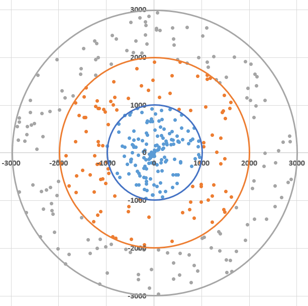
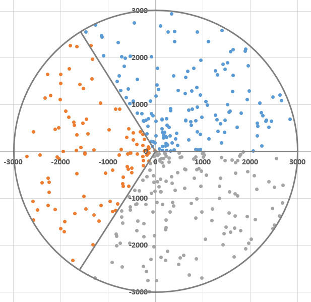
In the COR instances, we assume the commercial zone is the central circle with ray 1000, the residential zone is a ring in the middle around the commercial zone with outer ray 2000, and the industrial zone is a most outer ring around the residential zone with outer ray 3000. In the SEC instances, we assume that commercial, residential, and industrial zones correspond to three slices of identical size that partition a circle of ray 3000.
Then, for each zone, we uniformly generate the same number of demand nodes. More exactly, given the total number of demand nodes to be generated, such value is divided by three to obtain, after an integer rounding whenever necessary, the number of demand nodes to generate in each zone. Figure 2 gives an example.
Both in COR and SEC instances, a given number of potential stations is uniformly generated over the total area (i.e., the circle with ray 3000).
For each pair of demand node and potential station , parameter is computed as the Euclidean distance between the two nodes.
Concerning the demand pattern, this is specific for each zone. In the commercial zone we assume there is a high density of offices, shops, pubs, restaurants, and hotels. Hence, we expect a high demand with two peaks, the first one at the beginning of the working day and the second one in the afternoon, higher than the first peak and slowly decreasing in the evening hours. In the industrial zone, we expect a high demand in the morning with one peak around lunch time and an almost null demand during the night. Finally, in the residential zone, we assume the presence of a high density of private houses, with a comparatively low demand in the morning and a peak in the evening and early night hours. These assumptions are consistent with several studies regarding the spatial-temporal distribution of the charging demands observed in urban areas (see, e.g., Yi et al.,, 2020; Straub et al.,, 2021).
To generate the charging demand according to these patterns, we proceed as follows. We first generate three basic profiles of demand that mimic the patterns described above for the commercial, industrial, and residential zones, respectively. Such basic profiles are built according to the four standard demand levels shown in Table 1. The resulting basic demand profiles are depicted in Figure 3.
| Level | 0 | 1 | 2 | 3 |
|---|---|---|---|---|
| Demand | null | low | medium | high |
For each and , we randomly generate an initial demand value from a Poisson distribution with mean (and variance) equal to the standard level assigned to and in the corresponding basic profile. For example, if is in the commercial zone and , then is a realization of a Poisson with mean 2, cf. Figure 3(a). We then set:
where denotes the nearest integer rounding operator. In this way, we obtain that: (1) the total daily demand from each demand node is around 10; (2) the total demand in each zone is consistent with the corresponding basic demand profiles shown in Figure 3.


5.1.2 Remaining parameters
We generated a set of instances by varying the number of demand nodes , of potential stations , and of the maximum number of chargers to install in each station . All the remaining parameters take the same value across all instances. The name of each instance is , where:
-
✓
: The number of demand nodes ranges according to the following values: , 100, 150, 200, 250, and 500.
-
✓
: The number of potential stations ranges according to the following values: , 20, 30, 40, and 50.
-
✓
: The maximum number of chargers to install is equal across all the stations, and ranges according to the following values: , 20, and 30.
For example, instance 50_20_30 comprises 50 demand nodes, 20 potential stations, and parameter is equal to 30. Note that the latter parameter is equal for each potential station . We made this choice to simplify the interpretation of the results. For the same reason, we decided to set , for each and .
Each instance in our testbed has the following common characteristics:
-
✓
The planning horizon considered is 1 day, discretized in time periods of one hour length. Consequently, .
-
✓
The cost of opening one charging station is 100,000.
-
✓
Two types of chargers are considered. Therefore, , where 1 denotes quick chargers, and 2 stands for fast chargers.
-
✓
The cost of installing each type of chargers is and 25,000 for quick and fast chargers, respectively.
-
✓
Quick chargers need hours to fully recharge an EV, whereas fast chargers require hour. Parameter for the SP-CFL model is determined as: .
-
✓
The minimum percentage of chargers of each type to deploy in each zone is the following:
-
–
Commercial zone: at least 20% of quick chargers (), and at least 40% of fast chargers ().
-
–
Residential zone: at least 50% of quick chargers (), and at least 20% of fast chargers ().
-
–
Industrial zone: at least 25% of quick chargers (), and at least 25% of fast chargers ().
-
–
Note that, in both MILP models, the two components in the respective objective function can take very different values, differing even by orders of
magnitude. In our experiments we scaled the two components to make them
comparable in value.
We initially considered all possible combinations of the values mentioned above for , , and . Subsequently, we ruled out each instance that
turned out to be infeasible for both MILP models. This situation happened especially for the largest numbers of the demand nodes, the
smallest numbers of potential stations, and the smallest values of parameter . In such cases, the maximum charging capacity, obtained opening all
potential stations and deploying chargers in each station , turned out not to be sufficient to serve the total charging demand.
All together, we analyzed 67 instances.
5.2 A comparison between COR and SEC instances
To illustrate the solutions obtained by the two MILP models on the COR and SEC instances, we discuss the results obtained on two small instances. In both instances, the number of demand nodes is equal to 21, equally divided among the three zones. The number of potential stations is 5. We assumed that the planning horizon comprises 8 time periods, and that the demand profile in each zone is the one depicted in Figure 4. These profiles are the same for both the COR and SEC instance.


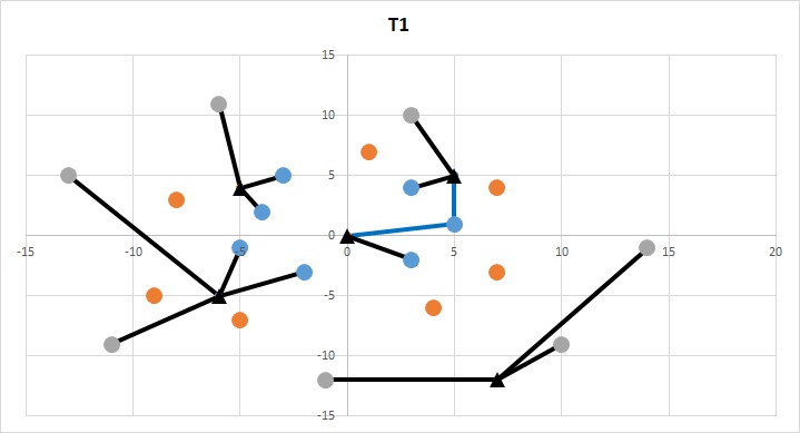
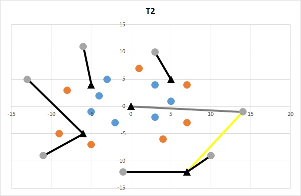
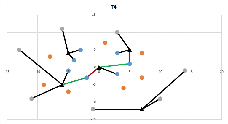
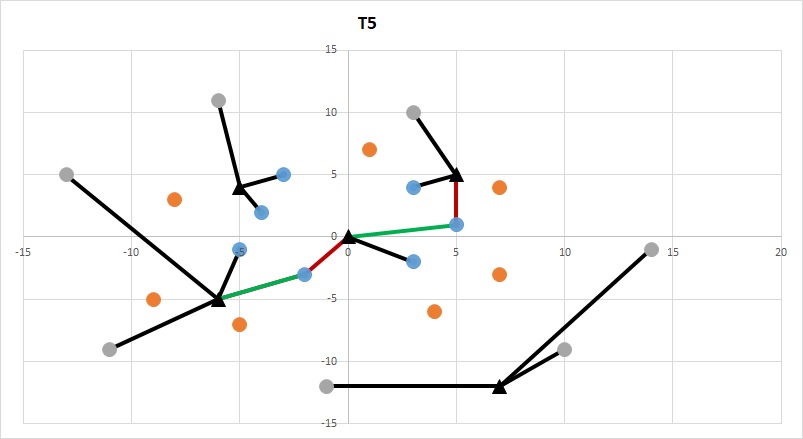
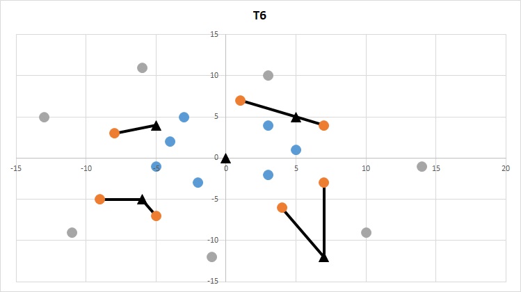
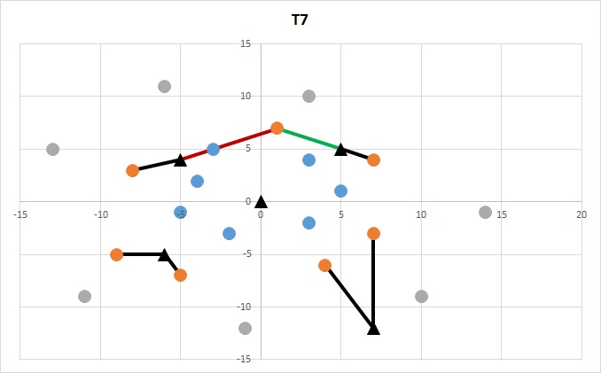
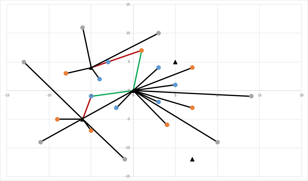
An optimal solution produced by the MP-CFL model for the COR instance is depicted in Figure 5, where demand nodes are colored circles (blue for the commercial zone, orange for the residential zone, grey for the industrial zone) and potential locations are black triangles. Moreover, the color of the edge connecting a demand node to a black triangle represents the fraction of the charging demand assigned to the station thereby opened (black = 100% of the demand, yellow 75%, red 66%, blue 50%, green 33% and gray 25%). Note that Figure 5 shows the assignments concerning only the significant time periods. In other words, the assignments in time periods 3 and 8 are not reported, the former since there is no demand in that time period, the latter because it is identical to time period 7. Figure 6 displays an optimal solution to the SP-CFL model for the same instance.
The optimal solutions found by the two MILP models for the SEC instance are shown in Figures 7 and 8.
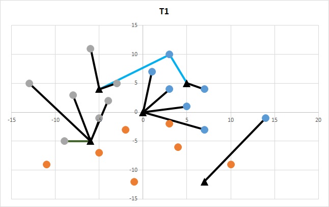
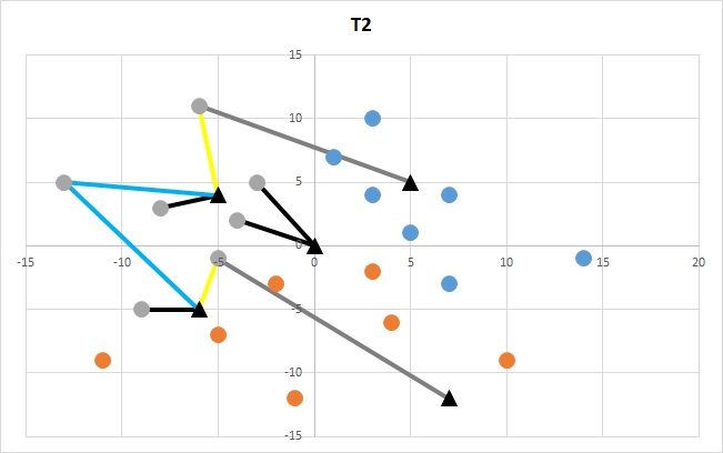
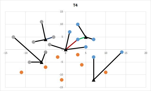
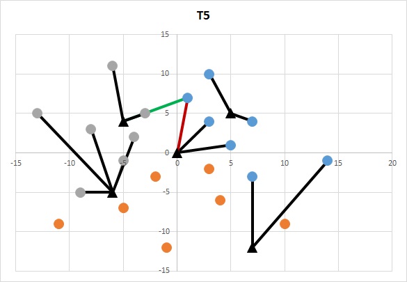
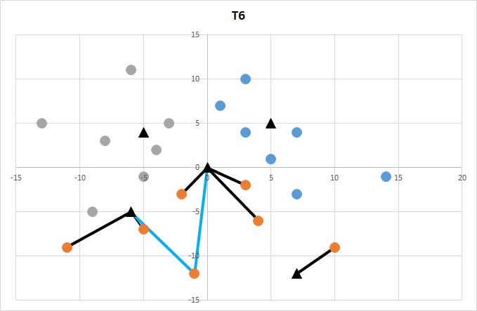
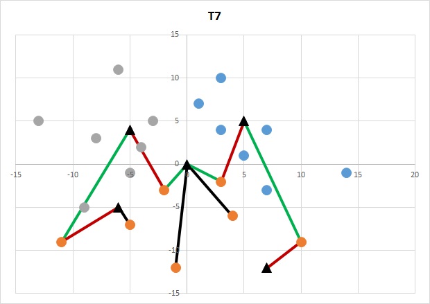
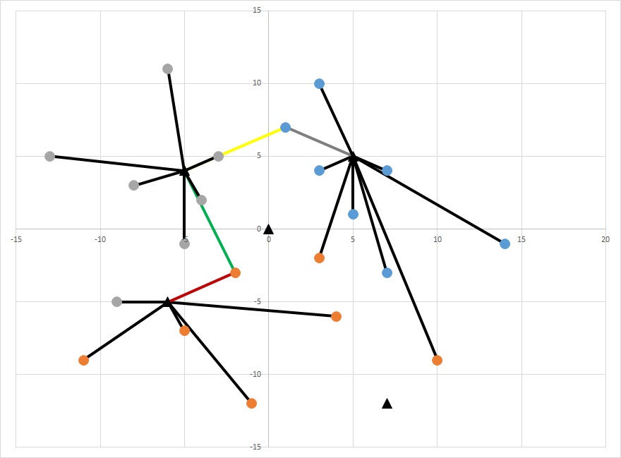
Comparing the optimal solutions for the COR instance obtained by the MP-CFL and the SP-CFL models (see Figures 5 and 6, respectively), one can notice that in the former all the potential stations are open and the charging demand is assigned, in the majority of the cases, to the nearest station. The solution found by the SP-CFL model opens only three stations. This small example highlights the limits of the latter model: it neglects that the charging demand is concentrated in few peak time periods, and, consequently, underestimates the charging need in those time periods. In fact, most of the demand is assigned to the charging station located in the central position (coordinates (0,0)), but the chargers deployed there are not sufficient to serve all the EVs during the peak hours. Due to the lower number of stations opened (3 against 5) and the number of chargers approximately 40% lower (30 against 52), we observe that 17.04% of customers cannot be served by the solution to SP-CFL.
Similar conclusions can be drawn observing the optimal solutions for the SEC instance produced by the MP-CFL and the SP-CFL models (see Figures 7 and 8, respectively). As expected, there is no remarkable difference between the computational time on the COR and SEC instances. To keep a reasonable length of the paper, we conducted the extensive experiments on the COR instances only.
5.3 Computational results
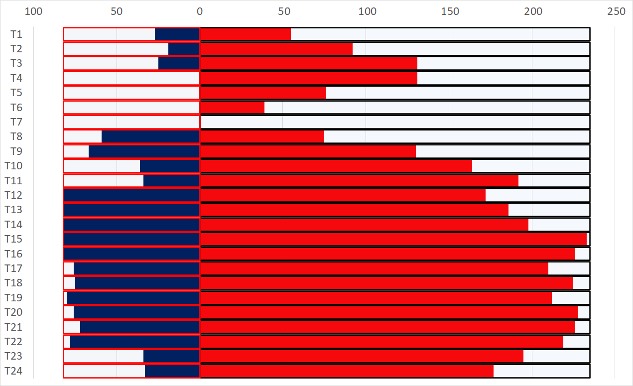
This section is devoted to the illustration and comment of the computational results. Before entering into the details of the results, we illustrate the solutions produced by the two MILP models for instance 200_30_30 and . Figure 9 depicts, for each time period, the charging capacity installed and the demand satisfied by an optimal solution to model MP-CFL for instance 200_30_30. For each time period (vertical axis), the tornado diagram shows as bordered bars the number of chargers of each type deployed: the red bordered bars (left) are the fast chargers, whereas the black bordered bars (right) are the quick chargers. The solid bars represent the assignment of the charging demand. For each time period and type of charger, the bar indicates the total number of chargers assigned to EVs. Recall that quick chargers need multiple time periods to fully charge an EV. Hence, an EV assigned to a quick charger will use it for multiple consecutive time periods. From Figure 9, one can notice that the demand assigned to each type of chargers in each time period does not violate the charging capacity deployed. Note also that in several time periods the demand approaches the capacity installed, and these two quantities are sometimes even equal (see the fast chargers in time periods 12 through 16).
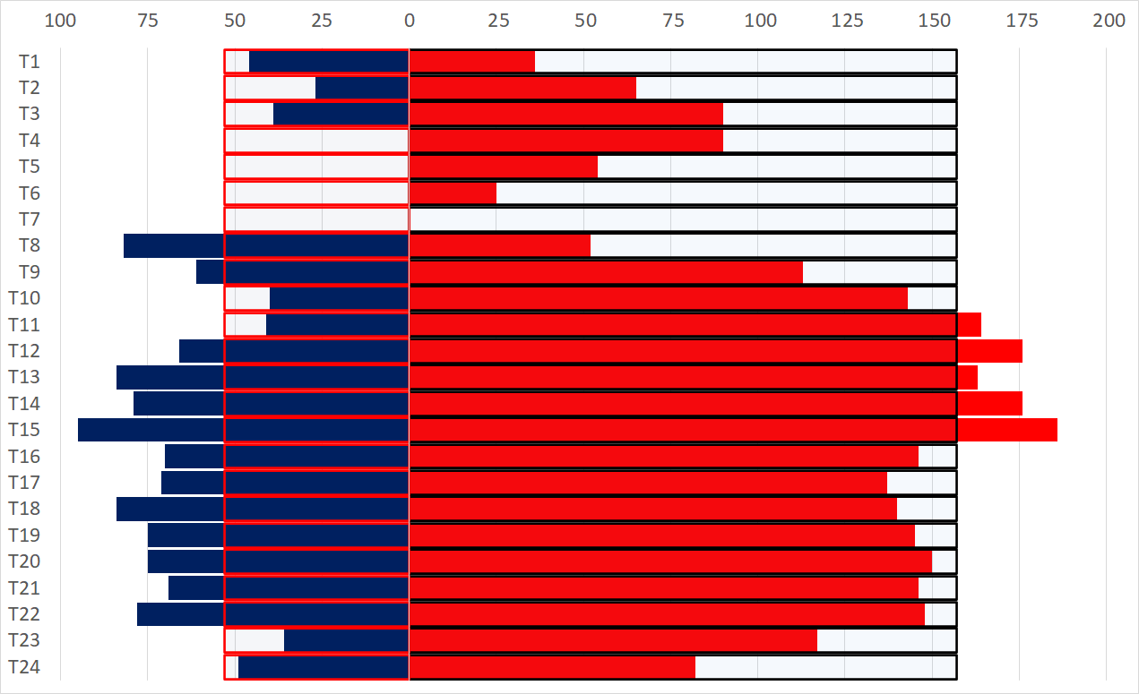
The limits of the solution produced by the SP-CFL model are evident from Figure 10. The solution found by the SP-CFL model assigns, in several time periods, more EVs than the chargers actually available. For the fast chargers, this happens in time periods 8, 9, and from 12 to 22. On the other hand, for the quick chargers, this occurs in time periods 11 through 15. We observed this outcome for the majority of the instances tested.
We now analyze more thoroughly the solutions produced by the two MILP models. To gain some insights about the two components of the objective functions, each instance is solved by each model for several values of the trade-off parameter . We tested the following values: (maximum weight on the minimization of the total opening and installing costs), 0.25, 0.5, 0.75, and 0.9999 (maximum weight on the minimization of the average distance traveled by the EVs).
Table 5.3 provides, in the first three groups of columns, a summary of the charging capacity deployed by the solutions found by the two MILP models. For each group of instances and each model, Table 5.3 shows the average number of stations open (columns with header “Stations”), as well as the average number of quick and fast chargers installed. For each value of , we reported in bold the average value of each of the former statistics for the MP-CFL model, along with the average deviation from the latter value for the SP-CFL model. The last group of three columns provides some statistics about the solution of the SP-CFL model. In fact, the statistics refer to a modified solution obtained as follows. The deployed capacity remains unchanged. However, as the solution assigns the demand to open stations that may be overloaded in some peak periods of time, we modified the assignment of the demand to the stations with the goal of increasing the percentage of demand satisfied by the charging capacity deployed by the solution to the SP-CFL model.
The procedure to modify the solution to the SP-CFL model iteratively considers one time period at a time, from 1 to , and, for a given time period , examines each demand node , from 1 to . The procedure checks whether the demand of node could be served in time period according to the assignment indicated by the values of variables . In this context, being served means that there is a number of vacant chargers in station greater than or equal to .
| Stations | Quick | Fast | SP-CFL | |||||||
|---|---|---|---|---|---|---|---|---|---|---|
| MP-CFL | SP-CFL | MP-CFL | SP-CFL | MP-CFL | SP-CFL | Reall% | Lost% | Max Lost% | ||
| 0.0001 | 50 | 4.33 | 2.67 | 53.33 | 33.00 | 23.33 | 15.00 | 6.37% | 21.00% | 60.23% |
| 100 | 8.20 | 5.00 | 101.07 | 60.53 | 45.87 | 30.40 | 9.82% | 21.07% | 58.33% | |
| 150 | 10.87 | 7.53 | 141.40 | 91.93 | 60.73 | 45.93 | 10.95% | 20.88% | 58.03% | |
| 200 | 14.64 | 9.71 | 186.00 | 126.50 | 94.14 | 61.00 | 10.41% | 21.10% | 58.60% | |
| 250 | 17.75 | 12.00 | 239.42 | 153.93 | 115.08 | 77.36 | 11.24% | 21.28% | 58.19% | |
| 500 | 31.25 | 21.64 | 418.56 | 300.18 | 198.78 | 154.82 | 13.24% | 21.82% | 55.89% | |
| Average | 12.90 | -28.93% | 171.01 | -30.32% | 80.46 | -25.87% | 10.19% | 21.16% | 58.32% | |
| 0.25 | 50 | 4.80 | 3.80 | 55.47 | 35.60 | 22.80 | 14.13 | 12.23% | 21.15% | 55.90% |
| 100 | 8.13 | 5.33 | 95.00 | 61.73 | 47.07 | 29.93 | 12.12% | 20.90% | 58.43% | |
| 150 | 11.07 | 7.73 | 137.00 | 90.13 | 68.57 | 46.07 | 11.66% | 20.98% | 57.90% | |
| 200 | 14.14 | 9.79 | 170.14 | 120.64 | 97.93 | 62.14 | 12.17% | 21.11% | 57.73% | |
| 250 | 17.50 | 11.79 | 227.58 | 143.21 | 117.75 | 79.79 | 12.54% | 21.35% | 54.93% | |
| 500 | 30.38 | 21.27 | 393.44 | 287.27 | 229.75 | 159.00 | 14.56% | 21.79% | 54.95% | |
| Average | 12.82 | -26.74% | 162.39 | -29.14% | 85.00 | -28.74% | 12.46% | 21.19% | 56.73% | |
| 0.50 | 50 | 6.93 | 6.60 | 62.67 | 36.60 | 23.20 | 14.40 | 18.38% | 19.64% | 54.65% |
| 100 | 8.67 | 7.60 | 97.73 | 73.67 | 46.20 | 27.00 | 14.02% | 20.56% | 62.05% | |
| 150 | 11.07 | 8.80 | 131.86 | 97.87 | 69.93 | 44.53 | 13.55% | 20.58% | 59.55% | |
| 200 | 14.21 | 10.71 | 166.71 | 126.29 | 98.86 | 60.86 | 13.93% | 20.82% | 58.03% | |
| 250 | 17.75 | 12.50 | 219.67 | 150.29 | 119.58 | 78.00 | 14.41% | 21.06% | 57.80% | |
| 500 | 30.88 | 21.55 | 441.50 | 285.73 | 230.50 | 158.82 | 16.00% | 21.69% | 54.80% | |
| Average | 13.44 | -19.64% | 163.51 | -26.20% | 85.68 | -30.81% | 14.86% | 20.68% | 57.95% | |
| 0.75 | 50 | 12.13 | 12.20 | 78.60 | 37.47 | 31.07 | 15.20 | 26.82% | 17.09% | 51.54% |
| 100 | 12.20 | 11.40 | 120.60 | 70.27 | 50.20 | 28.53 | 19.83% | 19.71% | 60.30% | |
| 150 | 13.64 | 12.80 | 152.93 | 103.73 | 73.14 | 43.00 | 18.00% | 20.06% | 60.58% | |
| 200 | 15.21 | 13.50 | 173.36 | 137.07 | 97.14 | 58.14 | 16.34% | 20.59% | 59.90% | |
| 250 | 18.00 | 14.79 | 223.25 | 156.71 | 120.58 | 76.43 | 16.13% | 20.88% | 58.69% | |
| 500 | 30.63 | 21.91 | 428.25 | 285.36 | 233.75 | 157.91 | 17.78% | 21.66% | 54.67% | |
| Average | 15.77 | -10.69% | 175.14 | -29.15% | 88.72 | -33.95% | 19.02% | 19.90% | 57.71% | |
| 0.9999 | 50 | 21.20 | 21.20 | 96.87 | 40.53 | 41.27 | 17.00 | 31.11% | 12.33% | 47.73% |
| 100 | 27.20 | 27.20 | 160.20 | 74.67 | 77.60 | 31.40 | 26.57% | 16.04% | 52.02% | |
| 150 | 29.71 | 28.40 | 212.93 | 104.33 | 113.86 | 46.87 | 24.51% | 16.62% | 57.10% | |
| 200 | 30.93 | 30.07 | 245.50 | 141.43 | 146.00 | 61.86 | 23.28% | 17.41% | 57.54% | |
| 250 | 33.58 | 30.79 | 276.00 | 165.29 | 158.29 | 79.43 | 22.05% | 17.92% | 57.05% | |
| 500 | 38.75 | 34.55 | 429.38 | 285.45 | 375.25 | 165.27 | 19.59% | 19.90% | 52.74% | |
| Average | 29.33 | -3.25% | 218.95 | -41.67% | 132.99 | -53.23% | 24.80% | 16.53% | 54.02% | |
If such demand cannot be completely served, the unserved demand is reallocated among the vacant chargers of any type different from available at the same station , if any. Then, the procedure attempts to reallocate the remaining unserved demand among the other stations. If there are vacant chargers among multiple stations, priority is given to the one nearest to . If at the station there are vacant chargers of multiple types, priority is given to the type that has the largest number of vacant units. Let be the demand arising in node at time period that the procedure has reallocated. Eventually, the procedure computes the fraction of the total demand that has been reallocated, in percentage, producing statistic “Reall%”. For each instance, the fraction of the total demand reallocated is computed as .
If, after the reallocation procedure, a portion of the demand is not served, the fraction of the total demand that remains unserved is computed, in percentage, producing statistic “Lost%”. For each instance, the latter is computed as , where is the demand arising in node at time period that is not served. Finally, the procedure computes statistic “Max Lost%” as the maximum fraction of demand not served across all time periods. The latter is computed for each instance as .
From Table 5.3 we can gain the following insights:
-
✓
the charging capacity deployed in the solutions to the SP-CFL model is significantly smaller than the capacity installed according to the MP-CFL model, both in terms of stations open and chargers installed (see statistics “Stations”, “Quick”, and “Fast”);
-
✓
reducing the weight of the opening and installing costs (i.e., increasing the value of ), the average deviation between the solutions to the two models in terms of stations open decreases steadily, from -28.93% for to -3.25% for . Nevertheless, the average number of chargers installed (of each type) in the solutions found by the SP-CFL model is always remarkably smaller compared to those produced by the MP-CFL model;
-
✓
given a value of , for both models the greater the number of demand nodes, the greater the number of stations open and chargers installed (see statistics “Stations”, “Quick”, and “Fast”);
-
✓
the larger the value of , the larger the values of “Stations”, “Quick”, and “Fast”. This is an expected outcome, as more importance is given to the average distance term in the objective functions. In other words, the reduction of the average distance traveled can only be achieved by increasing the number of stations opened and chargers deployed;
-
✓
due to the cheaper installation cost, both models install a larger number of quick compared to fast chargers.
Before entering into the details of the statistics computed to measure the limits of the SP-CFL model, it is worth pointing out that in every solution found by the latter model, a part of the demand was reallocated, and a part was lost. The main insights we can gain from the three rightmost columns of Table 5.3 are the following:
-
✓
“Reall%” takes, on average, large values. It ranges from 6.37% (see and ) to 31.11% (see and );
-
✓
“Lost%” takes, on average, large values as well. It ranges from 12.33% (see and ) to 21.82% (see and );
-
✓
“Max Lost%” takes, on average, extremely large values, always larger than 47%.
The statistics confirm that the SP-CFL model is not capable of capturing the characteristics of the problem and tends to underestimate the charging capacity to deploy.
Further insights that can be obtained from Table 5.3 on the limits of the SP-CFL model are as follows:
-
✓
for values of smaller than or equal to 0.25, the average value of “Reall%” tends to increase with the number of demand nodes;
-
✓
for values of greater than or equal to 0.75, the average value of “Reall%” tends to decrease with the number of demand nodes;
-
✓
the larger the value of , the larger the average value of “Reall%”, and the smaller tends to be the value of “Lost%”. This behavior can be explained by observing that increasing the value of , the number of stations opened and chargers installed increases as well, making it easier to find vacant chargers, and thereby reducing the unserved demand. of “Max Lost%” slightly decreases as the value of increases.
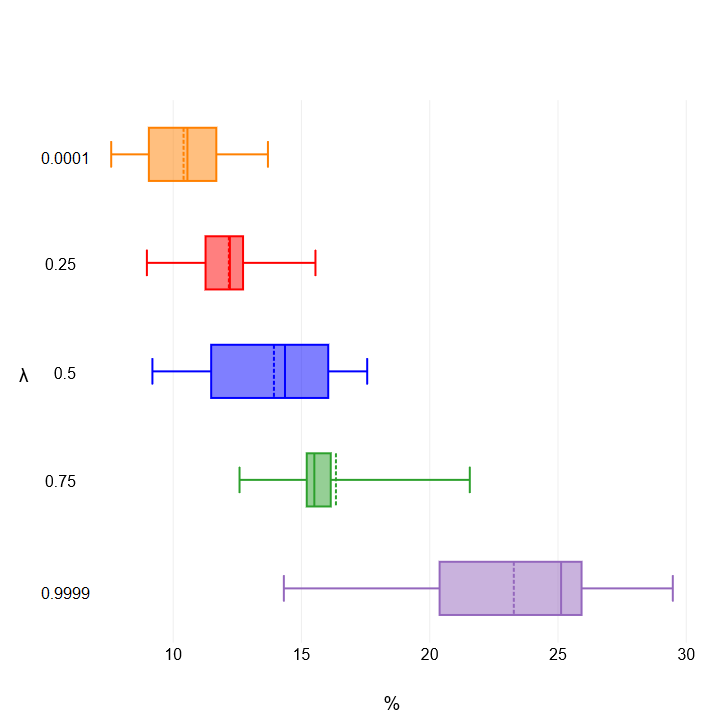
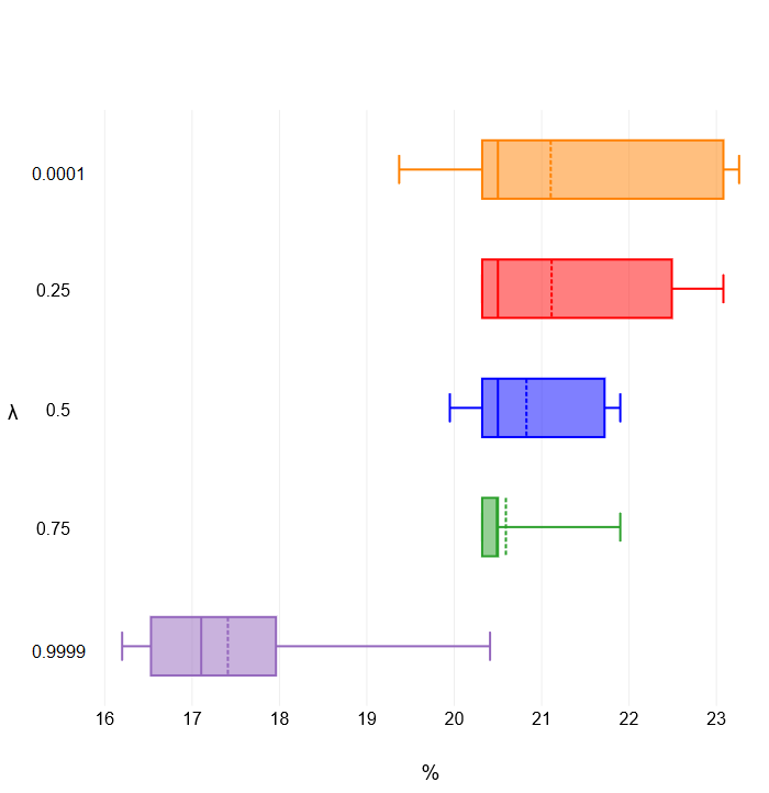
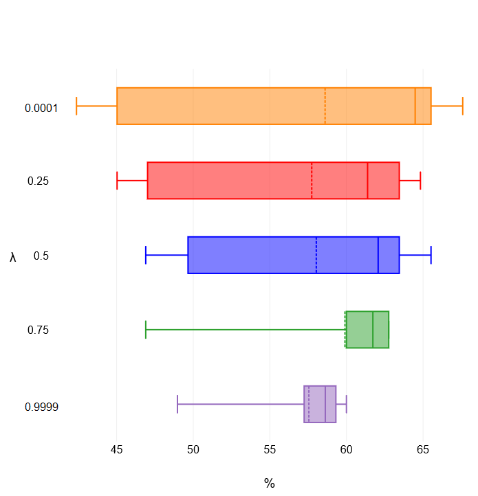
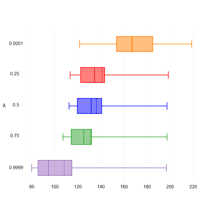
The box-and-whisker plots depicted in Figure 5.3 show the distribution of the values of the three statistics computed to determine the reallocated demand, and the unserved demand, for all the instances with solved for different values of . The box-and-whisker plots confirm the insights previously drawn. When the main term in the objective function of the SP-CFL model is the opening and installing cost - i.e, for small values of - the charging capacity installed is small and little can be done to reallocate the unserved demand. As a consequence, large percentages of the charging demand are unserved. By increasing the weight given to the average distance traveled - i.e., for large values of - the charging capacity installed increases. Consequently, the percentage of the demand that can be reallocated increases, and, thereby, the percentage of the demand that is unserved becomes smaller. Nevertheless, the latter percentages always remain quite large (the values are always greater than 16%, and often greater than 20%). The performance is even worse if we analyze the distribution of “Max Lost%”. Its average value ranges from approximately 56% to roughly 60% (see the dotted lines inside the boxes). Similar conclusions can be drawn observing the results obtained when solving the instances with a different number of demand nodes. For the sake of readability, such results are not reported here.
The results discussed above clearly show that the solutions found by the SP-CFL model, if implemented, would lead to a very poor quality of service provided to the EV drivers. Moreover, the results on demand reallocation imply that the objective function of SP-CFL would underestimate the total travel distance covered by the EV drivers to reach a free charging station.
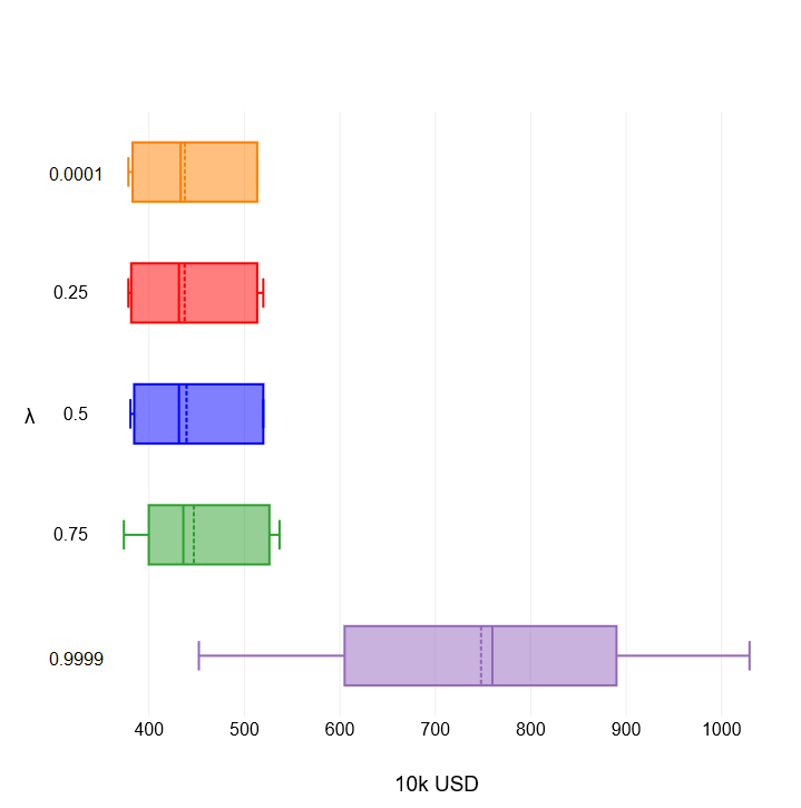
The following analysis is focused only on the solutions of the MP-CFL model. Figure 12 illustrates the distributions of the values of the average distance traveled (first term in the objective function) and the opening and installing cost (second term), for all the instances with solved for different values of .
From Figure 12, we can draw the following main insights:
-
✓
as expected, the larger the value of , the smaller the average distance traveled by an EV to reach the assigned charger;
-
✓
besides its largest value, increasing the value of produces only slight increases in the values of the total cost.
In fact, we expected a sharper increase of the values of the total cost when less importance is given to the second term of the objective function. On the contrary, and neglecting the extreme case with , when the value of is increased the solutions obtained by the MP-CFL model significantly improved the average traveling distance, at the cost of only a small deterioration of the total opening and installing cost.
We conclude our analysis by considering the computational burden required to solve each MILP model. Recall that each instance is solved with a time limit of 3,600 seconds. Table 3 summarizes the computational performance of the two MILP models. For each value of , the instances are clustered in groups according to the number of potential locations . For each group of instances and each model, Table 3 provides the average CPU time (in seconds) spent to find the optimal (or best) solution (columns with header “CPU Time (secs.)”), the average optimality gap (“Gap%”) and the worst optimality gap (“Max Gap%”).
The main insights that we can gain from Table 3 are as follows:
-
✓
the solution to the MP-CFL model is, in general, more computationally expensive compared to the SP-CFL model (see the average values of “CPU Time (secs.)”, and the average values of “Gap%”);
-
✓
the optimality gaps, for both models, are on average very small. In the majority of the cases, the solver found an optimal solution, or a solution very close to the optimum;
-
✓
the worst gaps, for both models, are also very small. In only few instances, statistic “Max Gap%” took a value greater than 1%;
-
✓
as expected, for a given value of , computing times for both models increase with the number of potential locations;
-
✓
the computational burden required to solve each MILP model decreases as the value of increases.
In summary, while the MP-CFL model requires on average more computational time than the SP-CFL model, the additional time needed by the MP-CFL model is marginally small.
| CPU Time (secs.) | Gap% | Max Gap% | |||||
|---|---|---|---|---|---|---|---|
| MP-CFL | SP-CFL | MP-CFL | SP-CFL | MP-CFL | SP-CFL | ||
| 0.0001 | 10 | 1,456.48 | 820.60 | 0.13% | 0.09% | 0.45% | 0.76% |
| 20 | 2,775.72 | 2,404.48 | 0.61% | 0.46% | 1.85% | 1.87% | |
| 30 | 3,308.19 | 2,759.82 | 1.03% | 1.08% | 2.90% | 3.69% | |
| 40 | 3,515.42 | 3,142.17 | 0.94% | 1.23% | 2.90% | 3.69% | |
| 50 | 3,513.11 | 3,330.17 | 1.08% | 1.43% | 2.90% | 3.69% | |
| Average | 3,037.11 | 2,568.85 | 0.81% | 0.90% | |||
| 0.25 | 10 | 660.83 | 259.72 | 0.03% | 0.01% | 0.17% | 0.11% |
| 20 | 2,133.02 | 922.11 | 0.12% | 0.04% | 0.60% | 0.37% | |
| 30 | 2,923.03 | 1,320.37 | 0.31% | 0.13% | 0.92% | 0.82% | |
| 40 | 3,156.36 | 1,790.20 | 0.45% | 0.19% | 1.19% | 1.07% | |
| 50 | 3,406.24 | 2,120.10 | 0.55% | 0.18% | 1.77% | 0.84% | |
| Average | 2,614.44 | 1,335.04 | 0.32% | 0.11% | |||
| 0.50 | 10 | 263.90 | 2.43 | 0.00% | 0.00% | 0.00% | 0.00% |
| 20 | 1,135.25 | 338.01 | 0.01% | 0.01% | 0.06% | 0.17% | |
| 30 | 2,544.90 | 1,334.12 | 0.19% | 0.07% | 0.67% | 0.66% | |
| 40 | 2,739.82 | 2,051.00 | 0.34% | 0.09% | 1.06% | 0.58% | |
| 50 | 2,978.22 | 2,145.28 | 0.97% | 0.10% | 6.85% | 0.49% | |
| Average | 2,094.62 | 1,238.01 | 0.34% | 0.06% | |||
| 0.75 | 10 | 6.45 | 2.51 | 0.00% | 0.00% | 0.00% | 0.00% |
| 20 | 376.49 | 1,183.04 | 0.00% | 0.01% | 0.02% | 0.13% | |
| 30 | 1,678.43 | 1,984.19 | 0.04% | 0.05% | 0.41% | 0.22% | |
| 40 | 2,449.72 | 2,298.07 | 0.06% | 0.07% | 0.37% | 0.24% | |
| 50 | 2,926.84 | 2,312.06 | 0.40% | 0.06% | 4.28% | 0.22% | |
| Average | 1,648.46 | 1,629.29 | 0.11% | 0.04% | |||
| 0.9999 | 10 | 2.80 | 1.97 | 0.00% | 0.00% | 0.00% | 0.00% |
| 20 | 966.18 | 1,488.73 | 0.00% | 0.00% | 0.00% | 0.00% | |
| 30 | 1,575.65 | 2,581.28 | 0.00% | 0.00% | 0.00% | 0.00% | |
| 40 | 1,864.13 | 3,243.86 | 0.00% | 0.00% | 0.00% | 0.00% | |
| 50 | 2,569.15 | 2,957.01 | 0.00% | 0.00% | 0.00% | 0.00% | |
| Average | 1,528.78 | 2,152.78 | 0.00% | 0.00% | |||
6 Conclusions
In this paper, we studied the role of temporal and spatial distributions of charging demand in determining an optimal location of charging stations for electrical vehicles in an urban setting. This is an application context where the daily demand is well-known to be very dynamic and concentrated at some peak hours, and where the demand pattern is known to depend also upon the city zone.
To highlight the need of considering explicitly the daily demand patterns, we presented a multi-period optimization model, that captures the variability over time of the demand, and compared it with a single-period optimization model. By means of a worst-case analysis, we theoretically proved that the single-period model may produce solutions where a large portion of the demand cannot be served. Extensive computational experiments confirm the limits of the single-period model. The goal of the optimization models is to balance two objectives: the total cost of deploying the infrastructure and the average distance traveled by the customers to reach a charging station.
The limits pointed out for the single-period model go beyond the specific application considered in this paper, and suggest the importance of incorporating time-dependency in location decisions when the demand fluctuations are remarkable during the planning horizon.
Future developments of the research may concern the objective function. Since the two objectives considered are not homogeneous, a thorough analysis of the trade-off between infrastructure cost and drivers traveling distance may be of interest to a decision-maker. Moreover, we expect that replacing the average traveling distance with some equity measures may produce solutions that are more satisfactory for the customers, at the cost of a little increase in the infrastructure cost. Finally, to solve larger instances, in particular when an equity measure is considered, a heuristic approach would deserve to be studied.
Acknowledgements
This study has been made in the framework of the MoSoRe@UniBS (Infrastrutture e servizi per la Mobilità Sostenibile e Resiliente) Project 2020-2022 of Lombardy Region, Italy (Call-Hub ID 1180965; bit.ly/2Xh2Nfr, https://ricerca2.unibs.it/?page id=8548).
References
- Anjos et al., (2020) Anjos, M. F., Gendron, B., and Joyce-Moniz, M. (2020). Increasing electric vehicle adoption through the optimal deployment of fast-charging stations for local and long-distance travel. European Journal of Operational Research, 285(1):263–278.
- Bekli et al., (2021) Bekli, S., Boyacı, B., and Zografos, K. G. (2021). Enhancing the performance of one-way electric carsharing systems through the optimum deployment of fast chargers. Transportation Research Part B: Methodological, 152:118–139.
- Brandstätter et al., (2017) Brandstätter, G., Kahr, M., and Leitner, M. (2017). Determining optimal locations for charging stations of electric car-sharing systems under stochastic demand. Transportation Research Part B: Methodological, 104:17–35.
- Brandstätter et al., (2020) Brandstätter, G., Leitner, M., and Ljubić, I. (2020). Location of charging stations in electric car sharing systems. Transportation Science, 54(5):1408–1438.
- Burgess, (2008) Burgess, E. W. (2008). The growth of the city: An introduction to a research project. In Urban Ecology, pages 71–78. Springer.
- Cavadas et al., (2015) Cavadas, J., de Almeida Correia, G. H., and Gouveia, J. (2015). A MIP model for locating slow-charging stations for electric vehicles in urban areas accounting for driver tours. Transportation Research Part E: Logistics and Transportation Review, 75:188–201.
- Deb et al., (2018) Deb, S., Tammi, K., Kalita, K., and Mahanta, P. (2018). Review of recent trends in charging infrastructure planning for electric vehicles. Wiley Interdisciplinary Reviews: Energy and Environment, 7(6):e306.
- Dong et al., (2019) Dong, G., Ma, J., Wei, R., and Haycox, J. (2019). Electric vehicle charging point placement optimisation by exploiting spatial statistics and maximal coverage location models. Transportation Research Part D: Transport and Environment, 67:77–88.
- Filippi et al., (2021) Filippi, C., Guastaroba, G., and Speranza, M. G. (2021). On single-source capacitated facility location with cost and fairness objectives. European Journal of Operational Research, 289(3):959–974.
- Hall and Barrett, (2012) Hall, T. and Barrett, H. (2012). Urban Geography. Routledge.
- Hosseini et al., (2017) Hosseini, M., MirHassani, S. A., and Hooshmand, F. (2017). Deviation-flow refueling location problem with capacitated facilities: Model and algorithm. Transportation Research Part D: Transport and Environment, 54:269–281.
- Hoyt, (1939) Hoyt, H. (1939). The structure and growth of residential neighborhoods in American cities. US Government Printing Office.
- Huang et al., (2016) Huang, K., Kanaroglou, P., and Zhang, X. (2016). The design of electric vehicle charging network. Transportation Research Part D: Transport and Environment, 49:1–17.
- Kchaou-Boujelben, (2021) Kchaou-Boujelben, M. (2021). Charging station location problem: A comprehensive review on models and solution approaches. Transportation Research Part C: Emerging Technologies, 132:103376.
- Kuby and Lim, (2005) Kuby, M. and Lim, S. (2005). The flow-refueling location problem for alternative-fuel vehicles. Socio-Economic Planning Sciences, 39(2):125–145.
- Laporte et al., (2019) Laporte, G., Nickel, S., and Saldanha-da Gama, F. (2019). Introduction to location science. In Laporte, G., Nickel, S., and Saldanha-da Gama, F., editors, Location science, pages 1–21. Springer.
- Li and Jenn, (2022) Li, X. and Jenn, A. (2022). An integrated optimization platform for spatial-temporal modeling of electric vehicle charging infrastructure. Transportation Research Part D: Transport and Environment, 104:103177.
- MirHassani and Ebrazi, (2013) MirHassani, S. and Ebrazi, R. (2013). A flexible reformulation of the refueling station location problem. Transportation Science, 47(4):617–628.
- Moloughney, (2021) Moloughney, T. (2021). What are the different levels of electric vehicle charging? https://www.forbes.com/wheels/advice/ev-charging-levels/ (Last accessed: 15th November 2022).
- Pareek et al., (2020) Pareek, S., Sujil, A., Ratra, S., and Kumar, R. (2020). Electric vehicle charging station challenges and opportunities: A future perspective. In 2020 International Conference on Emerging Trends in Communication, Control and Computing (ICONC3), pages 1–6. IEEE.
- Pevec et al., (2020) Pevec, D., Babic, J., Carvalho, A., Ghiassi-Farrokhfal, Y., Ketter, W., and Podobnik, V. (2020). A survey-based assessment of how existing and potential electric vehicle owners perceive range anxiety. Journal of Cleaner Production, 276:122779.
- Quddus et al., (2019) Quddus, M. A., Kabli, M., and Marufuzzaman, M. (2019). Modeling electric vehicle charging station expansion with an integration of renewable energy and Vehicle-to-Grid sources. Transportation Research Part E: Logistics and Transportation Review, 128:251–279.
- Rajabi-Ghahnavieh and Sadeghi-Barzani, (2017) Rajabi-Ghahnavieh, A. and Sadeghi-Barzani, P. (2017). Optimal zonal fast-charging station placement considering urban traffic circulation. IEEE Transactions on Vehicular Technology, 66(1):45–56.
- Straub et al., (2021) Straub, F., Streppel, S., and Göhlich, D. (2021). Methodology for estimating the spatial and temporal power demand of private electric vehicles for an entire urban region using open data. Energies, 14(8):2081.
- Wolbertus et al., (2018) Wolbertus, R., Kroesen, M., Van Den Hoed, R., and Chorus, C. (2018). Fully charged: An empirical study into the factors that influence connection times at EV-charging stations. Energy Policy, 123:1–7.
- Yi et al., (2020) Yi, T., Zhang, C., Lin, T., and Liu, J. (2020). Research on the spatial-temporal distribution of electric vehicle charging load demand: A case study in China. Journal of Cleaner Production, 242:118457.
- Yıldız et al., (2016) Yıldız, B., Arslan, O., and Karaşan, O. E. (2016). A branch and price approach for routing and refueling station location model. European Journal of Operational Research, 248(3):815–826.
- Zhang et al., (2019) Zhang, Y., Liu, X., Zhang, T., and Gu, Z. (2019). Review of the electric vehicle charging station location problem. In Wang, G., Bhuiyan, M. Z. A., De Capitani di Vimercati, S., and Ren, Y., editors, Dependability in Sensor, Cloud, and Big Data Systems and Applications, DependSys 2019, CCIS 1123, pages 435–445, Singapore. Springer Singapore.
- Zhu et al., (2016) Zhu, Z.-H., Gao, Z.-Y., Zheng, J.-F., and Du, H.-M. (2016). Charging station location problem of plug-in electric vehicles. Journal of Transport Geography, 52:11–22.