Chemical kinetics and stochastic differential equations

Abstract

We propose a general stochastic formalism for describing the evolution of chemical reactions involving a finite number of molecules. This approach is consistent with the statistical analysis based on the Chemical Master Equation, and provides the formal setting for the existing algorithmic approaches (Gillespie algorithm). Some practical advantages of this formulation are addressed, and several examples are discussed pointing out the connection with quantum transitions (radiative interactions).

All the chemical physical processes involve, in an atomistic perspective, a stochastic description of the events, be them reactive or associated with a change of phase (for instance adsorption) chemfluct . Nonetheless, in the overwhelming majority of the cases of practical and laboratory interest, the number of molecules involved is so large to justify a mean field approach, essentially based on the Boltzmannian hypothesis of molecular chaos (the “stosszahlansatz”) boltzmann . The mean field formulation represents the backbone of the classical theory of chemical reaction kinetics chemkin1 ; chemkin2 .

It is well known that, in all the cases where the number of molecule is small (and this occurs in subcellular biochemical reactions, in nanoscale systems, or in the growth kinetics of microorganisms bio1 ; bio2 ; bio3 ), the effects of fluctuations become significant, motivating a stochastic description of chemical kinetic processes, involving the number of molecules present in the system, thus explicitly accounting for due to their finite number mcquarrie ; stoca ; stoca1 ; stoca2 . The statistical theory of chemical kinetics in these conditions is grounded on the Chemical Master Equation (CME) gillespierigorous ; cme3 , expressing the evolution equation for the probabilities $p({\bf N},t)$ of all the possible number-configurations ${\bf N}(t)=(N_{1}(t),\dots,N_{s}(t))$, where $N_{h}(t)$ is the number of molecules of the $h$-th reacting species at time $t$, $h=1,\dots,s$. However, apart from a handful of simple cases, for which the CME can be solved analytically cmecpl , numerical methods should be applied to it in order to compute mean values and higher-order moments. But also this choice reveals itself to be unfeasible in most of the situations of practical and theoretical interests, due to the extremely large number of configurations involved, making the multi-index matrix $p({\bf N},t)$ so huge to exceed reasonable computational facilities.

In order to solve this problem, Gillespie proposed an algorithmic solution to the numerical simulation of stochastic reacting systems, based on the Markovian nature of the reactive events gillespiegeneral ; gillespieexamples . The original Gillespie algorithm has been extended and improved over time, providing a variety of slightly different computational alternatives. A common denominator of the first family of the Gillespie algorithms (namely those based on the direct method, the first reaction method or their derivates ff1 ; ff2 ; ff3 ) is to associate to every time step the occurrence of just one reaction. This formulation comes directly from the assumption that, if the time step is small enough, the probability that more than one reaction will occur is negligible. While correct, this choice brings to significant computational costs for complex reaction schemes. This problem has been highlighted several times, from the Gillespie group itself, as stiffness in stochastic chemical reacting systems stiffness . A brilliant way to overcome this limit originates the famous tau-leaping method, which, unfortunately, requires to check that the propensity functions remain almost constant at each iteration and can be applied just if this condition is verified tau1 ; tau2 . The algorithmic solution associated with the formalism here introduced combines the accuracy of the first SSA with the computational advantages of the $\tau$-leaping method.

There is, moreover, a missing link between the CME theory and the Gillespie algorithm, consisting in the straight mathematical formulation of the stochastic differential equations associated with a chemical reacting system, the statistical description of which would correspond to the CME. To clarify this issue, consider the conceptually analogous problem of particle diffusion over the real line, the statistical description of which is expressed by the parabolic equation $\partial p(x,t)/\partial t=D\,\partial^{2}p(x,t)/\partial x^{2}$, for the probability density $p(x,t)$ of finding a particle at position $x$ at time $t$. Setting $x_{n}=x(n\,\Delta t)$, an algorithm describing this process can be simply expressed by the discrete evolution equation $x_{n+1}=x_{n}+\sqrt{2\,D\,\Delta t}\,r_{n+1}$, where $r_{h}$, $h=1,2,\dots$ represent independent random variables sampled from a normal distribution (with zero mean, and unit variance) diffusion . This represents an efficient algorithmic solution of the problem, whenever the time resolution $\Delta t$ is small enough. Nevertheless, the mere algorithmic approach cannot be considered physically satisfactory, in a comprehensive formulation of transport theory embedded in a continuous space-time (in which both position $x$ and time $t$ are real valued). In point of fact, only with the mathematical formulation due to K. Ito of stochastic differential equations driven by the increments $dw(t)$ of a Wiener process (Langevin equations) ito , namely $dx(t)=\sqrt{2\,D}\,dw(t)$ the theory of diffusive motion has found a proper mathematical physical setting.

A similar situation applies to the case of stochastic models of chemical reaction kinetics, and the present Letter is aimed at filling this gap. The basic idea is that any reactive process corresponds to a system of elementary events (the single reaction) possessing a Markovian transitional structure, and, consequently, amenable to a description by means of the increments of counting processes (Poisson processes, in the Markovian case). This topic has been also pointed out in closed1 in terms of Poisson measures, although the latter formulation is much less simple and physically intuitive than the approach proposed in the present Letter.

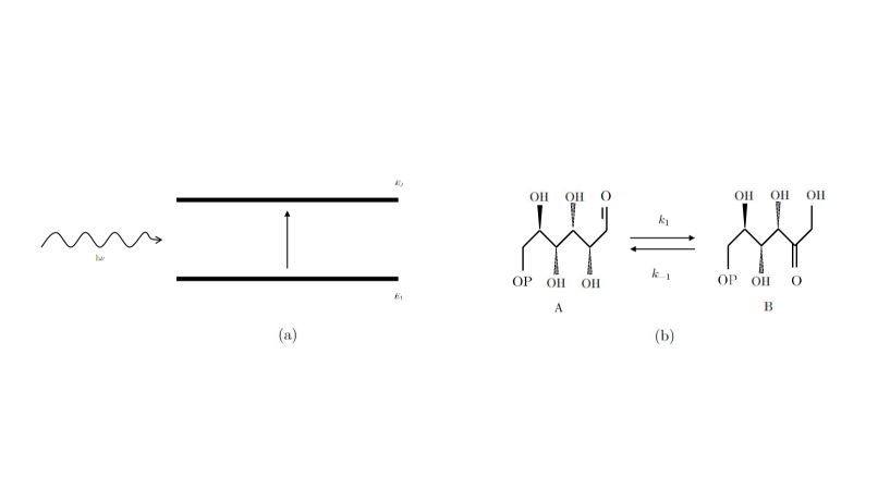
To begin with, consider the simple case of a first-order chemical reaction $A\underset{k_{-1}}{\stackrel{{\scriptstyle k_{1}}}{{\rightleftharpoons}}}B$ (for instance, an isomerization). This model is perfectly analogous to the radiative transition of a molecule possessing two energy states, due to emission and adsorption of an energy quantum (figure 1). Let $N_{A}(0)+N_{B}(0)=N_{g}$ the total number of molecules at time $t=0$. The state of the system is characterized by the state functions $\sigma_{h}(t)$, $h=1,\dots,N_{g}$ for each molecule, attaining values $\{0,1\}$, and such that $\sigma_{h}(t)=0$ if the energy state at time $t$ is $E_{0}$ (or equivalently if the molecule finds itself in the state $A$), and $\sigma_{h}(t)=1$ in the opposite case (energy state $E_{1}$, or isomeric state $B$).

Figure 1: Schematic representation of the analogy between a two-level quantum system and a first-order chemical kinetics, such as an isomerization.

Let $\{\chi_{h}^{(1)}(t,k_{1}),\chi_{h}^{(2)}(t,k_{-1})\}_{h=1}^{N_{g}}$ be two systems of independent Poisson processes, characterized by the transition rates $k_{1}$, and $k_{-1}$, respectively. The evolution of $\sigma_{h}(t)$ can be expressed via the stochastic differential equation

$$\frac{d\sigma_{h}(t)}{dt}=\left(1-\sigma_{h}(t)\right)\,\frac{d\chi_{h}^{(1)}(t,k_{1})}{dt}-\sigma_{h}(t)\,\frac{d\chi_{h}^{(2)}(t,k_{-1})}{dt}$$ (1)

$h=1,\dots,N_{g}$, where $d\chi(t,\lambda)/dt$ is the distributional derivative of the Poisson process $\chi(t,\lambda)$, corresponding to a sequence of unit impulsive functions at the transition instants $t_{i}^{*}$, $i=1,2,\dots$, $0<t_{i}^{*}<t_{i+1}^{*}$, where for $\varepsilon>0$, $\lim_{\varepsilon\rightarrow 0}\int_{t_{i}^{*}-\varepsilon}^{t_{i}^{*}+\varepsilon}d\chi(t,\lambda)=1$. Summing over $h=1,\dots N_{g}$, and observing that $N_{A}(t)=\sum_{h=1}^{N_{g}}\left(1-\sigma_{h}(t)\right)$, $N_{B}(t)=\sum_{h=1}^{N_{g}}\sigma_{h}(t)$, we have

$$\frac{dN_{B}(t)}{dt}=\sum_{h=1}^{N_{A}(t)}\frac{d\chi_{h}^{(1)}(t,k_{1})}{dt}-\sum_{h=1}^{N_{B}(t)}\frac{d\chi_{h}^{(2)}(t,k_{-1})}{dt}$$ (2)

and $dN_{A}(t)/dt=-dN_{B}(t)/dt$, representing the evolution equation for $N_{A}(t)$ and $N_{B}(t)$, attaining integer values. The stochastic evolution of the number of molecules $N_{A}(t)$, $N_{B}(t)$ is thus expressed as a differential equation with respect to the continuous physical time $t\in{\mathbb{R}}^{+}$, over the increments of a Poisson process. Intepreted in a mean-field way, if $c_{\rm tot}$ is the overall concentration of the reactants at time $t=0$, then the concentrations $c_{\alpha}(t)$ at time $t$ can be recovered from eq. (2) as

$$c_{\alpha}(t)=c_{\rm tot}\,\frac{N_{\alpha}(t)}{N_{g}}\,,\qquad\alpha=A,B$$ (3)

representing the calibration relation connecting the stochastic description in terms of number of molecules $N_{\alpha}(t)$ and the concentrations $c_{\alpha}(t)$, $\alpha=A,\,B$ entering the mean-field description.

The analytical formulation of a stochastic differential equation for chemical kinetics, expressed in terms of the number of molecules of the chemical species involved, rather than an algorithm defined for discretized times, permits to develop a variety of different numerical strategies, that naturally perform a modified tau-leaping procedure, as the occurrence of several distinct reactive events in any elementary time step $\Delta t$ is intrinsically accounted for. This can be easily seen by considering the simple reaction defined by the evolution equation (2). In terms of increments, eq. (2) can be written as $dN_{B}(t)=\sum_{h=1}^{N_{A}(t)}d\chi^{(1)}(t,k_{1})-\sum_{h=1}^{N_{B}(t)}d\chi^{(2)}(t,k_{-1})$. If $\Delta t$ is the chosen time step, it follows from this formulation, a simple numerical approximation for eq. (2), namely,

$$\Delta N_{B}(t)=N_{B}(t+\Delta t)-N_{B}(t)=\sum_{h=1}^{N_{A}(t)}\xi_{h}^{(1)}(k_{1}\,\Delta t)-\sum_{h=1}^{N_{B}(t)}\xi_{h}^{(2)}(k_{-1}\,\Delta t)$$ (4)

where $\xi^{(1)}(k_{1}\,\Delta t)$, $\xi_{h}^{(2)}(k_{-1}\,\Delta t)$ $h=1,2,\dots$, are two families of independent binary random variables, where

$$\xi^{(\alpha)}_{h}(p)=\left\{\begin{array}[]{lll}1&&\mbox{with probability}\;p\\ 0&&\mbox{otherwise}\end{array}\right.$$ (5)

$\alpha=1,2$, $h=1,2,\dots$. The time step $\Delta t$, can be chosen in eq. (4) from the condition

$$K\,\Delta t<1\,,\qquad K=\max\{k_{1},k_{-1}\}$$ (6)

In practice, we choose $\Delta t=0.1/K$. As can be observed, the choice of $\Delta t$ is limited by the intrinsic rates of the process. The advantage of deriving different algorithmic schemes for solving numerically the stochastic kinetic equations becomes more evident in dealing with bimolecular reactions (addressed below). Due to the intrinsic limitations of this communication, a thorouh discussion of this issue is postponed to a future more extensive article PG_next .

The same approach can be extended to include amongst the elementary events not only the reactive steps, but also feeding conditions, thus representing the evolution of chemically reacting systems with a finite number of molecules in a perfectly stirred open reactor. This is the case of the tank-loading problem, in which a tracer is injected in an open vessel assumed perfectly mixed, for which, in the absence of chemical reactions, the mean field equation for the concentration of the tracer reads

$$\frac{dc(t)}{dt}=D\,\left(c_{0}-c(t)\right)$$ (7)

where $c_{0}$ is the inlet concentration and $D$ the dilution rate (reciprocal of the mean retention time), and $c(0)=0$. Fixing $N_{g}$ so that $c(t)=c_{0}\,N(t)/N_{g}$, the corresponding stochastic differential equation for the integer $N(t)$ involves, also in this case, two families of counting processes, one for the loading at constant concentration $c_{0}$, and the other for tracer discharge in the outlet stream, characterized by the same transition rate $D$,

$$\frac{dN(t)}{dt}=\sum_{h=1}^{N_{g}}\frac{d\chi_{h}^{(1)}(t,D)}{dt}-\sum_{k=1}^{N(t)}\frac{d\chi_{h}^{(2)}(t,D)}{dt}$$ (8)

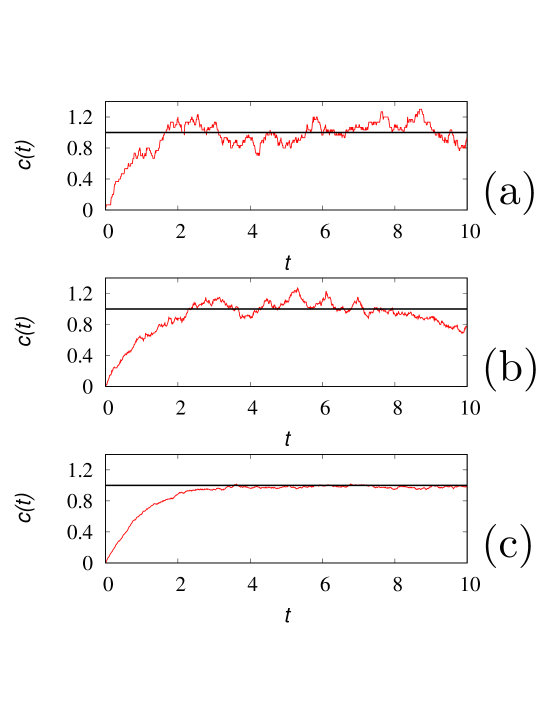
starting from $N(0)=0$. Figure 2 depicts several realizations of the tank-loading process, obtained by discretizing eq. (8) with a time step $\Delta t=10^{-3}$.

Figure 2: $c(t)=N(t)/N_{g}$ vs $t$ from a single realization of the tank-loading process eq. (8) with $D=1$, $c_{0}=1$ a.u.. Panel (a): $N_{g}=30$, panel (b) $N_{g}=100$, panel (c) $N_{g}=1000$. The solid horizontal lines represent the steady-state value $c^{*}=1$.

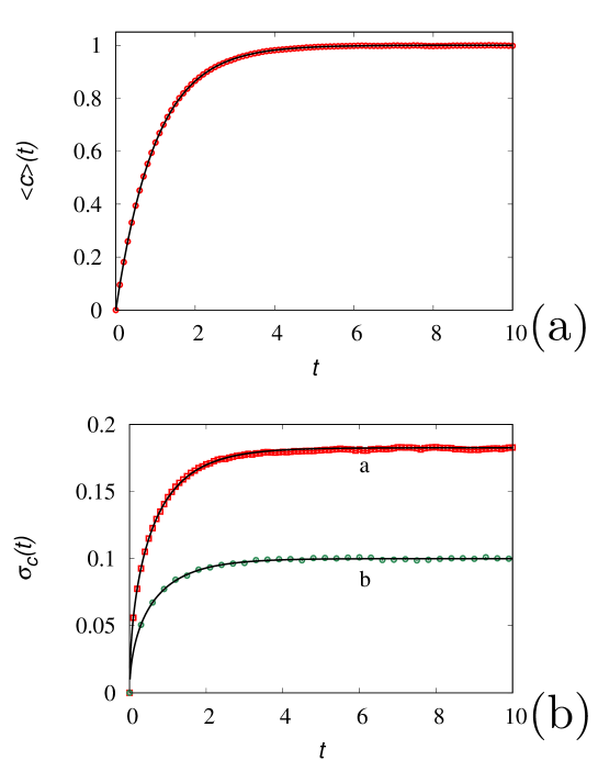
Despite the simplicity of the process, this example permits to highlight the role of $N_{g}$, that can be referred to as the granularity number, and the way stochastic models of chemical reactions can be fruitfully applied. Indeed, there is a two-fold use of the stochastic formulation of chemical kinetic schemes. The first refers to a chemical reacting system involving a small number of molecules, and in this case $N_{g}$ represents the effective number of molecules present in the system. The other is to use stochastic algorithms for simulating reacting systems in an alternative (and sometimes more efficient way) with respect to the solution of the corresponding mean-field equations. In the latter case, the granularity number $N_{g}$ represents essentially a computational parameter, tuning the intensity of the fluctuations. Two choices are then possible: (i) it can be chosen large enough, in order to obtain from a single realization of the process an accurate approximation of the mean-field behavior, or (ii) it can be chosen small enough in order, to deal with extremely fast simulations of a single realization of the process, that could be averaged over a statistically significant number of realizations in due time. These two choices are depicted in figure 2 (panel c), choosing $N_{g}=10^{3}$, and in figure 3 panel (a) obtained for $N_{g}=30$. Of course, the latter approach is valid as long as the low-granularity (low values of $N_{g}$) does not influence the qualitative properties of the kinetics.

Figure 3: Panel (a): $\langle c\rangle(t)$ vs $t$ at $N_{g}=30$ (symbols) averaged over $[10^{6}/N_{g}]$ realizations of the tank-loading process with $D=1$, $c_{0}=1$ a.u. Here, $[\cdot]$ indicates the integer part of its argument. The solid line represents the mean-field result $\langle c\rangle(t)=1-e^{-t}$. Panel (b): Variance $\sigma_{c}(t)$ vs $t$ for the tank-loading process. Symbols are the results of stochastic simulations of eq. (8) averaged over $[10^{6}/N_{g}]$ realizations, lines the solutions of eq. (10). Line (a) refers to $N_{g}=30$, line (b) to $N_{g}=100$.

The second (computational) use of stochastic simulations of chemical kinetics requires a further discussion. At a first sight, it may appear that any stochastic simulation would be computationally less efficient than the solution of the corresponding mean-field equations. This is certainly true for classical chemical reaction schemes in a perfectly mixed system, for which the mean-field model reduces to a system of ordinary differential equations for the concentrations of the reactants. But there are kinetic problems e.g., associated with the growth of microorganisms and eukaryotic cell lines in bioreactors (these growth phenomena, are indeed amenable to a description in terms of equivalent chemical reactions), the mean-field model of which is expressed in the form of higher-dimensional nonlinear integro-differential equations . For this class of problems, the use of stochastic simulations is the most efficient, if not the only way to achieve a quantitative description of the process, in those cases where the number $n_{p}$ of internal parameters describing the physiological state of an eukaryotic cell becomes large enough, $n_{p}\geq 3$. This issue is addressed in detail in PBGbio . This case is altogether similar to some transport problems, such as Taylor-Aris dispersion for high Péclet numbers or the analysis of microfluidic separation processes (DLD devices) for which the stochastic simulation of particle motion is far more efficient that the corresponding solution of the corresponding mean-field model expressed in the form of advection-diffusion equations taris ; dld .

To complete the analysis of the tank-loading problem, the associated CME reads

$$\frac{dp(n,t)}{dt}=D\,N_{g}\,\left[p(n-1,t)\,\eta_{n-1}-p(n,t)\right]+D\left[(n+1)\,p(n+1,t)-n\,p(n,t)\right]$$ (9)

where $\eta_{h}=1$ for $h\geq 0$ and $\eta_{h}=0$ otherwise. It follows that $\langle c\rangle(t)=c_{0}\sum_{n=1}^{\infty}n\,p(n,t)/N_{g}$ satisfies identically the mean-field equation (due to the linearity of the problem), while the variance $\sigma_{c}(t)$, with $\sigma_{c}^{2}(t)=c_{0}^{2}\sum_{n=1}^{\infty}n^{2}\,p(n,t)/N_{g}^{2}-\left(c_{0}\sum_{n=1}^{\infty}n\,p(n,t)/N_{g}\right)^{2}$, satisfies the equation

$$\frac{d\sigma_{c}^{2}}{dt}=-2\,D\,\sigma_{c}^{2}+D\,\left(\frac{1}{N_{g}}+\frac{\langle c\rangle}{N_{g}}\right)$$ (10)

Figure 3 panel (b) compares the results of stochastic simulations against the solutions of eq. (10) for two values of $N_{g}$.

The above approach can be extended to any system of nonlinear reaction schemes involving unimolecular and bimolecular reaction, and in the presence of slow/fast kinetics. The structure of the reaction mechanism can be arbitrarily complicated without adding any further complexity (other than purely notational) in the formulation of the stochastic evolution expressed in terms of number of molecules. The only practical issue, is that the number of different families of stochastic processes grows with the number of elementary reactive processes considered. For instance, in the case of the subtrate-inhibited Michaelin-Menten kinetics

$$E+S\underset{k_{-1}}{\stackrel{{\scriptstyle k_{1}}}{{\rightleftharpoons}}}ES$$

$$ES\overset{k_{2}}{\rightarrow}E+P$$ (11)

$$ES+S\underset{k_{-3}}{\stackrel{{\scriptstyle k_{3}}}{{\rightleftharpoons}}}ESS$$

there are five reactive processes (five channels in the language of the Gillespie algorithm) and consequently five families of counting processes $\{\chi_{i_{h}}^{(h)}(t,\cdot)\}$, $h=1,\dots,5$, should be introduced, so that the formulation of the discrete stochastic dynamics reads

$$\frac{dN_{S}(t)}{dt} = -\sum_{i=1}^{N_{S}(t)}\frac{d\chi_{i}^{(1)}(t,\widetilde{k}_{1}\,N_{E}(t))}{dt}+\sum_{j=1}^{N_{ES}(t)}\frac{d\chi_{j}^{(2)}(t,k_{-1})}{dt}$$

$$\frac{dN_{E}(t)}{dt} = -\sum_{i=1}^{N_{S}(t)}\frac{d\chi_{i}^{(1)}(t,\widetilde{k}_{1}\,N_{E}(t))}{dt}+\sum_{j=1}^{N_{ES}(t)}\frac{d\chi_{j}^{(2)}(t,k_{-1})}{dt}+\sum_{h=1}^{N_{ES}(t)}\frac{d\chi_{h}^{(3)}(t,k_{2})}{dt}$$

$$\frac{dN_{ES}(t)}{dt} = \sum_{i=1}^{N_{S}(t)}\frac{d\chi_{i}^{(1)}(t,\widetilde{k}_{1}\,N_{E}(t))}{dt}-\sum_{j=1}^{N_{ES}(t)}\frac{d\chi_{j}^{(2)}(t,k_{-1})}{dt}-\sum_{h=1}^{N_{ES}(t)}\frac{d\chi_{h}^{(3)}(t,k_{2})}{dt}-\sum_{k=1}^{N_{S}(t)}\frac{d\chi_{k}^{(4)}(t,\widetilde{k}_{3}\,N_{ES}(t))}{dt}$$ (12)

$$+ \sum_{l=1}^{N_{ESS}(t)}\frac{d\chi_{l}^{(5)}(t,k_{-3})}{dt}$$

$$\frac{dN_{ESS}(t)}{dt} = \sum_{k=1}^{N_{S}(t)}\frac{d\chi_{k}^{(4)}(t,\widetilde{k}_{3}\,N_{ES}(t))}{dt}-\sum_{l=1}^{N_{ESS}(t)}\frac{d\chi_{l}^{(5)}(t,k_{-3})}{dt}$$

$$\frac{dN_{P}(t)}{dt} = \sum_{h=1}^{N_{ES}(t)}\frac{d\chi_{h}^{(3)}(t,k_{2})}{dt}$$

equipped with the initial conditions $c_{S}(0)=c_{S,0}$, $c_{E}(0)=c_{E,0}$, $c_{ES}(0)=c_{ESS}(0)=c_{P}(0)=0$. Observe that for the bimolecular steps we have used a number-dependent rate coefficient. This is just one possibility, out of other fully equivalent alternatives, of defining bimolecular reacting processes, and out of tem a numerical algorithm for solving them. This issue, and its computational implications will be addressed elsewhere PG_next . The granularity number $N_{g}$ can be fixed, so that

$$N_{S}(0)=[c_{S,0}\,N_{g}]\,,\qquad N_{E,0}=[c_{E,0}\,N_{g}]$$ (13)

where $[\xi]$ indicates the integer part of $\xi$, thus defining the relation betwen $N_{\alpha}(t)$ and $c_{\alpha}(t)$, namely $c_{\alpha}(t)=N_{\alpha}(t)/N_{g}$, $\alpha=S,\,E,\,ES,\,ESS,\,P$. This implies also that the effective rate parameters entering the discrete stochastic evolution equation (12), and associated with the two bimolecular reactive steps, are given by $\widetilde{k}_{1}=k_{1}/N_{g}$, and $\widetilde{k}_{3}=k_{3}/N_{g}$.

Consider the case $k_{-1}=k_{2}=k_{3}=k_{-3}=1$, $c_{S,0}=4$, $c_{E,0}=0.1$. In this case the quasi steady-state approximation of the $c_{ES}$-$c_{S}$ curve (representing the slow manifold of the kinetics takes the expression

$$c_{ES}=\frac{c_{E,0}\,c_{S}}{K_{M}+c_{S}+\beta\,c_{S}^{2}}\,,\qquad K_{M}=\frac{k_{-1}+k_{2}}{k_{1}}\,,\quad\beta=\frac{k_{-3}}{k_{3}}$$ (14)

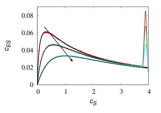
Figure 4 depicts the $c_{ES}$-$c_{S}$ graph obtained from a single realization of the stochastic process eq. (11) at several values of $k_{1}$ so as to modify the Michaelis-Menten constant $K_{M}$ for a value $N_{g}=10^{6}$ of the granularity number.

Apart from the initial transient giving rise to an overshot in the values of $c_{ES}$ near $c_{S}\simeq c_{S,0}$, the dynamics rapidly collapses towards the slow manifold and the stochastic simulations at high $N_{g}$-value provide a reliable description of the mean-field behavior starting from a single stochastic realization.

Figure 4: $c_{ES}$ vs $c_{S}$ plot of the substrate-inhibited enzymatic kinetics discussed in the main text. Symbols (in color) are the results of stochastic simulations of a single realization of the process eq. (11), (black) solid lines the graph of the quasi steady-state approximation. The arrow indicates increasing values of $K_{M}$, i.e. decreasing values of $k_{1}=20,\,6,\,2$.

To conclude, we want to point out some advantages and extensions of the present approach:

• it shows a direct analogy between chemical reaction kinetics, radiative processes and stochastic formulation of open quantum systems, thus, paving the way for a unified treatment of the interpaly between these phenomena, that is particularly important in the field of photochemistry, and in the foundation of statistical physics PGradia ; petruccione ;

• it can be easily extended to semi-Markov transition. This is indeed the case of the growth kinetics of eukaryotic microorganisms, the physiological state of which can be parametrized with respect to internal (hidden) parameters such as the age, the cytoplasmatic content, etc.;

• it can be easily extended to include transport phenomena. In point of fact, the occurrence of Markovian or semi-Markovian transitions in modeling chemical kinetics is analogous to the transitions occurring in the direction of motion (Poisson-Kac processes, Lévy flights, Extended Poisson-Kac processes) or in the velocity (linearized Boltzmannian schemes) GPK ; EPK ; Levy .

• it is closely related to the formulation of stochastic differential equations for the thermalization of athermal system athermo1 , in which the classical mesoscopic description of thermal fluctuations, using the increments of a Wiener process, is replaced by a dynamic model involving the increments of a counting process.

Due to the limitations of a Letter, all these issues will be addressed in forthcoming works. But apart for these extensions and improvements, the proposed formulation indicates that the stochastic theory of chemical reactions can be built upon a simple and consistent mathematical formalism describing the elementary reactive events as Markovian or semi-Markovian counting processes semimarkovcounting , that perfectly fits with the description of molecular non reactive events (molecular collisions), providing an unifying stochastic formalism of elementary (classical and quantum) molecular events.

References

- (1) P. L. Krapivsky, S. Redner, E. Ben-Naim, A Kinetic View to Statistical Physics, Cambridge University Press, Cambridge (2010).
- (2) L. Boltzmann, Weitere Studien ber das Wrmeglichgenicht unter Gas-moleklen, Sitzungsberichte Akademie der Wissenschaften 66 (1872) 275-370.
- (3) G. B. Marin, G. S. Yablonsky, D. Constales, Kinetics of chemical reactions: decoding complexity, John Wiley & Sons, New York, (2019).
- (4) O. Levenspiel, Chemical Reaction Engineering, J. Wiley & Sons (1998).
- (5) Z. Wang, Z. Hou, H. Xin, Internal noise stochastic resonance of synthetic gene network, Chemical Physics Letters, 401 (1-3) (2005) 307-311.
- (6) M. Perc, M. Gosak, and M. Marhl, From stochasticity to determinism in the collective dynamics of diffusively coupled cells, Chemical Physics Letters, 421 (1-3) (2006) 106–110.
- (7) G. Lente, A binomial stochastic kinetic approach to the michaelis–menten mechanism, Chemical Physics Letters, 568 (2013) 167–169.
- (8) D. A. McQuarrie, Stochastic approach to chemical kinetics, Journal of Applied Probability, 4 (3) (1967) 413-478.
- (9) D. T. Gillespie, Stochastic simulation of chemical kinetics, Annual Review of Physical Chemistry 58 (1) (2007) 35-55.
- (10) M. Delbrück, Statistical fluctuations in autocatalytic reactions, The Journal of Chemical Physics 8 (1) (1940) 120-124.
- (11) A. F. Bartholomay, A stochastic approach to statistical kinetics with application to enzyme kinetics, Biochemistry 1 (2) (1962) 223-230.
- (12) D. T. Gillespie, A rigorous derivation of the chemical master equation, Physica A 188 (1-3) (1992) 404-425.
- (13) J. Keizer, On the necessity of using the master equation to describe the chemical reaction , Chemical Physics Letters, 10 (4) (1971) 371–374.
- (14) B. J. Gaynor, R. G. Gilbert, K. D. King, Solution of the master equation for unimolecular reactions, Chemical Physics Letters, 55 (1) (1978) 40-43.
- (15) D. T. Gillespie, A general method for numerically simulating the stochastic time evolution of coupled chemical reactions, Journal of Computational Physics 22 (4) (1976) 403-434.
- (16) D. T. Gillespie, Exact stochastic simulation of coupled chemical reactions, The Journal of Physical Chemistry 81 (25) (1977) 2340-2361.
- (17) M. A. Gibson, J. Bruck, Efficient exact stochastic simulation of chemical systems with many species and many channels, The Journal of Physical Chemistry A 104 (9) (2000) 1876-1889.
- (18) L. Lok , R. Brent, Automatic generation of cellular reaction networks with Moleculizer, Nature Biotechnology 23 (2005) 131–36
- (19) Y. Cao, H. Li,L. R. Petzold, Efficient formulation of the stochastic simulation algorithm for chemically reacting systems, The Journal of Chemical Physics 121 (2004) 4059–67.
- (20) M. Rathinam, L. R. Petzold, Y. Cao, D. T. Gillespie, Stiffness in stochastic chemically reacting systems: The implicit tau-leaping method, The Journal of Chemical Physics, 119 (24) (2003) 12784-12794.
- (21) C. Yang, D. T. Gillespie, L. R. Petzold, Efficient step size selection for the tau-leaping simulation method, The Journal of Chemical Physics 124 (4) (2006) 044109.
- (22) C. Yang, D. T. Gillespie, L. R. Petzold, Adaptive explicit-implicit tau-leaping method with automatic tau selection, The Journal of Chemical Physics 126 (22) (2007) 224101.
- (23) D. C. Venerus and H. C. Öttinger, A modern Course in Transport Phenomena, Cambridge University Press, Cambridge (2018).
- (24) K. Ito and H. P. McKean Jr., Diffusion Processes and their Sample Paths, Springer, Berlin (1974).
- (25) F. Campillo, M. Chebbi, S. Toumi, Stochastic modeling for biotechnologies Anaerobic model AM2b, Revue Africaine de la de la Recherche en Informatique et Mathématiques Appliqués, INRIA 28 (2018 - 2019), Mathematics for Biology and the Environment 13-23.
- (26) C. Pezzotti, M. Giona, Stochastic chemical reactions: from algorithmic approaches to stochastic differential models, in preparation (2022).
- (27) C. Pezzotti, G. Procopio, A. Brasiello, M. Giona, Stochastic simulations of bioreactors in the presence of biomass heterogeneity and structured eukaryotic populations, in preparation (2022).
- (28) R. Aris, ”On the dispersion of a solute in a fluid flowing through a tube, Proceedings of the Royal Society of London A (235) (1956) 67-77.
- (29) S. Cerbelli, M. Giona, F. Garofalo, Quantifying dispersion of finite-sized particles in deterministic lateral displacement microflow separators through Brenner’s macrotransport paradigm, Microfluidics and nanofluidics 15 (2013) 431-449.
- (30) C. Pezzotti and M. Giona, Particle-photon radiative interactions and thermalization, in preperation (2022).
- (31) H.-P. Breuer, F. Petruccione, The Theory of Open Quantum Systems, Clarendon Press, Oxford (2002).
- (32) M. Giona, A. Brasiello, S. Crescitelli, Stochastic foundations of undulatory transport phenomena: Generalized Poisson–Kac processes—Part I basic theory, Journal of Physics A (50) (2017) 335002.
- (33) M. Giona, A. Cairoli, R. Klages, Extended Poisson-Kac theory: A unifying framework for stochastic processes with finite propagation velocity, Physical Review X (12) (2022) 021004.
- (34) K.-I. Sato, Lévy processes and infinitely divisible distributions, Cambridge University Press, Cambridge (1999).
- (35) K. Kanazawa, Statistical Mechanics for Athermal Fluctuation, Springer Nature, Singapore (2017).
- (36) D. Cocco, M. Giona, Generalized Counting Processes in a Stochastic Environment. Mathematics 9 (2021) 25-73.