Synchronization transitions on connectome graphs with external force

Abstract

We investigate the synchronization transition of the Shinomoto-Kuramoto model on networks of the fruit-fly and two large human connectomes. This model contains a force term, thus is capable of describing critical behavior in the presence of external excitation. By numerical solution we determine the crackling noise durations with and without thermal noise and show extended non-universal scaling tails characterized by $2<\tau_{t}<2.8$, in contrast with the Hopf transition of the Kuramoto model, without the force $\tau_{t}=3.1(1)$. Comparing the phase and frequency order parameters we find different transition points and fluctuations peaks as in case of the Kuramoto model. Using the local order parameter values we also determine the Hurst (phase) and $\beta$ (frequency) exponents and compare them with recent experimental results obtained by fMRI. We show that these exponents, characterizing the auto-correlations are smaller in the excited system than in the resting state and exhibit module dependence.

I Introduction

The critical brain hypothesis has been confirmed experimentally many times since the pioneering electrode experiments in Beggs and Plenz (2003). Power law (PL) distributed neuronal avalanches were shown in neuronal recordings (spiking activity and local field potentials, LFPs) of neural cultures in vitro Mazzoni et al. (2007); Pasquale et al. (2008); Friedman et al. (2012), LFP signals in vivo Hahn et al. (2010), field potentials and functional magnetic resonance imaging (fMRI) blood-oxygen-level-dependent (BOLD) signals in vivo Shriki et al. (2013); Tagliazucchi et al. (2012), voltage imaging in vivo Scott et al. (2014), $10$–$100$ and single-unit or multi-unit spiking and calcium-imaging activity in vivo Priesemann et al. (2014); Bellay et al. (2015); Hahn et al. (2017); Seshadri et al. (2018). Furthermore, source reconstructed magneto- and electroencephalographic recordings (MEG and EEG), characterizing the dynamics of ongoing cortical activity, have also shown nonuniveral PL scaling in neuronal long-range temporal correlations Palva et al. (2013); Fuscà et al. (2022). Optical methods, like light-sheet microscopy with GCaMP zebrafish larvae Ponce-Alvarez et al. (2018) or calcium imaging recordings of dissociated neuronal cultures Yaghoubi et al. (2018) also show PL scaling.

From a theoretical point of view the hypothesis is also very attractive as critical systems possess optimal computational capabilities as well as provide efficient long range communications, memory and sensitivity Chialvo and Bak (1999); Chialvo (2004, 2006, 2007); Chialvo et al. (2008); Fraiman et al. (2009); Expert et al. (2011); Fraiman and Chialvo (2012); Deco and Jirsa (2012); Deco et al. (2014); Senden et al. (2017); Muñoz (2018).

Homogeneous critical systems exhibit universal scaling behavior and many experiments claim indeed a mean-field class behavior of the branching process Plenz et al. (2021); Kinouchi and Copelli (2006) generated by self-organized criticality Bak et al. (1987). However, neural systems are very non-homogeneous, thus it is natural to expect non-universal behavior, known in statistical physics within the field of quenched disordered models Vojta (2006); Ódor et al. (2021). Indeed some experiments Palva et al. (2013); Fuscà et al. (2022); Yaghoubi et al. (2018) show that the measured exponents are not universal, significantly different from the mean-field class ones of the branching process.

Furthermore, external sources can move the system away from criticality Fosque et al. (2021) or tune it to other classes like the isotropic percolation Yaghoubi et al. (2018); Korchinski et al. (2021) or tricritical points Almeira et al. (2022). More complex models than the two-state branching process, can also exhibit hybrid type of phase transitions, like threshold models Ódor and de Simoni (2021), models with inhibitory nodes Corral López et al. (2022) or models with oscillatory units Buendía et al. (2021). Subsystems can also show different scaling behavior and may be within different distances from criticality Morales et al. (2022).

For quenched disordered models it has recently been shown Ye and Vojta (2022); Ódor (2019), that even for weak time dependence the semi-critical, dynamical scaling, which occurs in an extended control parameter region of criticality, in the so called Griffihts Phases Griffiths (1969) (GP), remains stable. Furthermore, even when the network dimension is high, one does not find the usual mean-field behavior, but in the presence of modules a GP Moretti and Muñoz (2013); Ódor et al. (2015); Cota et al. (2018); Ódor and de Simoni (2021); Korchinski et al. (2021); Buendí a et al. (2022) or Griffihts effects  Cota et al. (2016) and a different, sometimes logarithmically slow scaling at the critical point  Vojta (2006).

The big advantage of critical universality is that more realistic models for the brain, like the integrate and fire models Burkitt (2006), can also show the same criticality as simpler ones like in a recent work  Liang et al. (2020), which derives Hopf bifurcation criticality or in a more experimental study Orlandi et al. (2013) of neural cultures agreement with isotropic percolation avalanche size distributions is obtained. But of course the directed percolation criticality Janssen (1981); Grassberger (1982), which occurs in branching processes Beggs and Plenz (2003) is the main example for the universality principle Ódor (2008). Therefore, the study of simpler models, for which numerical analysis can be done are very useful for the brain science Muñoz (2018); Ódor et al. (2021).

Recently threshold models and Kuramoto type of models have been analyzed on different, available connectome networks and GP behavior was reported Ódor (2016, 2019); Ódor and Kelling (2019); Ódor et al. (2021, 2022, 2021). This behavior is also called as frustrated synchronization Villegas et al. (2014, 2016); Millán et al. (2018) and has been analyzed within the framework of a Kuramoto like models, albeit lacking quenched self-frequencies.

From the experimental directions the different behavior in modules of brains of the mouse Morales et al. (2022), by phenomenological renormalization-group analysis of the spectrum of electrode spikes, and humans Ochab et al. (2022), via Hurst and $\beta$ exponents analysis of fMRI; quasi-critical (off-critical) scaling like behavior has been shown. Here we attempt to model this using the Shinomoto–Kuramoto (SK) model on connectomes of the fruit-fly (FF) and humans. This is an extension of the Kuramoto model Kuramoto (2012), which itself does not have an external source, that can describe the resting state critical behavior at the Hopf transition towards a model with a periodic external driving force, thus may be appropriate to characterize criticality with an excitation Buendía et al. (2021).

II Models and methods

In this Section we introduce the synchronization model, followed by an overview of different connectome graphs, on which we run the numerical analysis. Finally we discuss the method of local synchronization to dig into the details of the spatio-temporal simulations of these brain systems.

II.1 The Shinomoto–Kuramoto (SK) model

We consider an extension of the Kuramoto model Kuramoto (2012) of interacting oscillators sitting at the nodes of a network, whose phases $\theta_{j}(t)$, $j=1,2\dots,N$ evolve according to the following set of dynamical equations

$$\dot{\theta}_{j}(t) = \omega_{j}^{0}+K\sum_{k}W_{jk}\sin[\theta_{k}(t)-\theta_{j}(t)]$$

$$+ F\sin(\theta_{j}(t))+\epsilon\eta_{j}(t)\ .$$

Here, $\omega_{j}^{0}$ is the so-called self-frequency of the $j$th oscillator, which is drawn from a Gaussian distribution with zero mean and unit variance. The summation is performed over adjacent nodes, coupled by the $W_{jk}$ matrix. Up to this point we have the classical Kuramoto model Kuramoto (2012). In the Shinomoto extension Shinomoto and Kuramoto (1986), we have a Gaussian annealed noise term $\eta_{j}(t)$, with an amplitude $\epsilon$, and to describe excitation, a site dependent periodic force term, proportional to a coupling $F$.

Sakaguchi Sakaguchi (1988) was the first to study the periodically forced Kuramoto model. In numerical simulations, however, he found that the state of forced entrainment was not always attained: macroscopic fractions of the system self-synchronized at a different frequency from that of the drive, indicating that this sub-population had broken away and established its own collective rhythm. Analytically improvements were provided in Antonsen et al. (2008); Ott and Antonsen (2008); Childs and Strogatz (2008) and found a rich phase space of the SK model.

Recently, in Buendía et al. (2021) the avalanche behavior of the full equation was investigated, albeit with site independent self-frequencies $\omega_{j}^{0}=\omega$. The authors explored the phase diagram, besides the forceless Hopf transition a so-called saddle node invariant cycle (SNIC) and a hybrid type of bifurcation was compered. In a very recent publication Buendí a et al. (2022) this numerical analysis has been continued on Erdős–Rényi (ER) and hierarchical modular networks, motivated by brain research. Considering quenched $\omega_{j}^{0}$-s with bi-modal frequency distributions the authors claim the emergence of Griffiths effects by the broadening of the synchronization transition region.

Here we study the SK model using quenched $\omega_{j}^{0}$-s with and without annealed noise $\eta_{j}(t)$ on real connectomes. In particular we test if the chaoticity, generated by the quenched $\omega_{j}^{0}$-s generates the same phase transition behavior and avalanches as with the presence of the stochastic noise. We measured the Kuramoto phase order parameter:

$$z(t)=r(t)\exp{i\theta(t)}=1/N\sum_{j}\exp{[i\theta_{j}(t)}]\ ,$$ (2)

by increasing the sampling time $\delta t=0.01$. Here $0\leq r(t)\leq 1$ gauges the overall coherence and $\theta(t)$ is the average phase. The set of equations (II.1) was solved by the steppers Runge–Kutta-4 (RK4), for the noisy, or by the Bulrisch–Stoer P. (1983); Hairer et al. (1987) (BS) for the noiseless cases, because in the presence of noise the adaptive BS fails to work. Here and in earlier studies Ódor et al. (2021) we found that the stronger stochastic noise makes the results non-reliable, while application of other steppers slow down the numerical solution. For the noisy cases we also tried the Euler–Maruyama solver Maruyama (1955), which has a stronger mathematical foundation for stochastic differential equations. This had to be restricted to testing purposes only, as this first-order solver is orders of magnitude slower than the RK4 for the same precision.

We integrated the set of equations numerically for $10^{3}-10^{4}$ independent initial conditions, by different $\omega_{j}^{0}$-s and sample averages of the phases

$$R(t)=\langle r(t)\rangle$$ (3)

and of the variance of the frequencies

$$\Omega(t)=\frac{1}{N}\sum_{j=1}^{N}(\overline{\omega}(t)-\omega_{j}^{2}(t))$$ (4)

were determined, where $N$ denotes the number of nodes.

In the steady state, which we determined by visual inspection of $R(t)$ and $\Omega(t)$, we measured their half values and the standard deviations: $\sigma(R(t))$, $\sigma(\Omega(t))$ in order to locate the transition points. Note, that $\sigma(R(t))$ is just a version of the SK order parameter employed by Lima Dias Pinto and Copelli (2019) for discrete version of oscillatory models. In case of the Kuramoto equation the fluctuations of both order parameters show a peak, albeit at different $K^{\prime}_{c}$ (for phases) and $K_{c}$ (for frequency) values in the case of the KKI-18 connectome. For graph dimensions $3<d<4$ a crossover transition is expected for $R$ and phase transition for $\Omega$. In the case of the FF, having $d>5$ we found $K_{c}\simeq K^{\prime}_{c}$, which is expected for real phase transitions at large sizes, where both order parameters converge to a finite value in the infinite size limit Ódor et al. (2022).

II.2 Connectome graphs

The connectome is defined as the structural network of neural connections in the brain Sporns et al. (2005). For the fruit-fly connectome, we used the hemibrain data-set (v1.0.1) from dow (2020), which has $N_{FF}=21\,662$ nodes and $L_{FF}=3\,413\,160$ edges, out of which the largest single connected component contains $N=21\,615$ and $L=3\,410\,247$ directed and weighted edges. The number of incoming edges varies between $1$ and $2708$. The weights are integer numbers, varying between $1$ and $4299$. The average node degree is $\langle k\rangle=315.129$ (for the in-degrees it is: $157.6$), while the average weighted degree is $\langle w\rangle=628$. The adjacency matrix, visualized in  Ódor et al. (2022) where one can see a rather homogeneous, almost structureless network, however it is not random. For example, the degree distribution is much wider than that of a random ER graph and exhibits a fat tail. The analysis in Ódor et al. (2022) found a weight distribution $p(w)$ with a heavy tail, assuming a PL form, an exponent $-2.9(2)$ could be fitted for the $w>100$ region.

The human brain has $\approx 10^{11}$ neurons, which current imaging techniques cannot comprehensively resolve at the scale of single neurons. We used graphs on the coarse-grained, level with $\approx 10^{6}$ nodes obtained by diffusion tensor imaging Landman et al. (2011). This method has generally been found to be in good agreement with ground-truth data from histological tract tracing Delettre et al. (2019). Inferred networks of structural connections were made available by the Open Connectome Project and previously analyzed by Gastner and Ódor (2016). These graphs are symmetric, weighted networks, where the weights measure the number of fiber tracts between nodes. The network topology study found a certain level of universality in the topological features of the ten large human connectomes investigated: degree distributions, graph dimensions, clustering and small world coefficients. These can be observed in Tables 3 and 4 of Gastner and Ódor (2016). Therefore, two networks, called KKI-18, and KKI-113 were selected to be the representatives in further studies. The graphs, downloaded in 2015 from the Open Connectome project repository OCP (2015), were generated via the MIGRAINE pipeline Gray Roncal et al. (2013), publicly available from m2g . KKI-18 comprises a large component with $N=804\,092$ nodes connected via $41\,523\,908$ undirected edges and several small disconnected sub-components, which were ignored in the modeling. Similarly, the extracted largest connected component of KKI-113 contains $799\,133$ nodes connected by $48\,096\,500$ undirected and weighted edges. The large number of nodes is because of other parcellations closer to voxel resolution being used. For instance, there are approximately 1.8 million voxels in the brain mask of a 1 mm resolution standard-aligned MRI. The graphs exhibit a hierarchical modular structure, because they are constructed from cerebral regions of the Desikan–Killany–Tourville parcellations, which is standard in neuroimaging Desikan et al. (2006); Klein and Tourville (2012) providing (at least) two different scales.

The modularity quotient of a network is defined by Newman (2006)

$$Q=\frac{1}{N\langle{k}\rangle}\sum\limits_{ij}\left(A_{ij}-\frac{k_{i}k_{j}}{N\langle{k}\rangle}\right)\delta(g_{i},g_{j}),$$ (5)

the maximum of this value characterizes how modular a network is, where $A_{ij}$ is the adjacency matrix, $k_{i}$, $k_{j}$ are the node degrees of $i$ and $j$ and $\delta(g_{i},g_{j})$ is $1$ when nodes $i$ and $j$ were found to be in the same community, or $0$ otherwise. However, this value is not independent of the community detection method. If our detection method produces lower modularity than the maximum achieved, it means our algorithm has fallen behind others. Community detection algorithms based on modularity optimization will get the closest to the actual modular properties of the network. We calculated the modularity using community structures detected by the Louvain method Blondel et al. (2008), the results for each network were: $Q_{FF}\approx 0.631,Q_{KKI-18}\approx 0.913,Q_{KKI-113}\approx 0.915$. The FF is a small-world network, according to the definition of the coefficient Humphries and Gurney (2008):

$$\sigma^{W}=\frac{C^{W}/C_{r}}{L/L_{r}}\ ,$$ (6)

because $\sigma_{FF}=9.5$ is much larger than unity. Here $C^{W}$ denotes the Watts clustering coefficient, and $L$ the average path length. $C_{r}$ and $L_{r}$ are the reference values of random networks with the same sizes and average degrees. The same is true for the human connectomes, as their $\sigma^{W}$ is in the range between $400$ and $1000$  Gastner and Ódor (2016).

The effective graph (topological) dimension, obtained by the breadth-first search algorithm is $d=5.4(5)$. This is defined by $N(r)\sim r^{d}$, where the number of nodes $N(r)$ with chemical distance $r$ or less from the seeds are counted and averages are calculated over the many trials. For the Open Connectome data, power-law fits in the range $1\leq r\leq 5$ suggest topological dimensions between $d=3$ and $d=4$ Gastner and Ódor (2016).

As these structural connectome graphs exhibit heavy-tailed weight distributions, probably as a result of learning, there exist hubs, which could fully determine the behavior of neighboring nodes and suppress the occurrence of critical behavior in the models Ódor (2016). In reality, on top of the structural weights, there exist inhibition/excitation mechanisms, which control the dynamics of the neural system and provide a local homeostasis. As we do not know the details of these mechanisms, in earlier studies Ódor (2016, 2019); Ódor and Kelling (2019); Ódor et al. (2021, 2022, 2021), the weight normalization scheme

$$W^{\prime}_{jk}=W_{jk}/\sum_{k}W_{jk}$$ (7)

was applied to achieve this artificially. This way we equalize the sensitivity of nodes to the incoming excitation. We do the same in the simulations presented here.

II.3 Analysis of the local synchronization

As the connectomes are very heterogeneous, built up from modules we also measured the local Kuramoto order parameter $R_{i}(t)$, defined as the partial sum of phases for the neighbors of node $i$

$$R_{i}(t)=\frac{1}{N_{\mathrm{i.neigh}}}\left|\sum_{j}^{N_{\mathrm{i.neigh}}}A_{ij}e^{i\theta_{j}(t)}\right|\ ,$$ (8)

and the local $\Omega_{i}(t)$ defined as

$$\Omega_{i}(t)=\frac{1}{N_{\mathrm{i.neigh}}}\left|\sum_{j}^{N_{\mathrm{i.neigh}}}(\overline{\omega}(t)-\omega_{j}(t))^{2}\right|\ .$$ (9)

The local Kuramoto order parameter was initially suggested by Restrepo et al. (2005); Schröder et al. (2017) to quantify the local synchronization of nodes, which allows us to follow the synchronization process by mapping the solutions on the connectome graphs.

The necessity of storing the states of the system at each time step requires large amount of hard drive storage. Thus we analyzed the local order parameters in a time period of $50$ time-steps as stop time with time increment of $dt^{\prime}=0.1$ , in the steady state. To study it in more detail we also separated the networks into communities. Although, these communities should be separated according to anatomical and/or functional properties Sanchez-Rodriguez et al. (2021), we chose as a first approximation a community detection method based on global optimization of the modularity Blondel et al. (2008). This method yielded 9 modules in FF network, 130 communities in KKI-113 and 134 modules in the giant component of KKI-18. For detecting community structure that is closer to the real anatomical functional communities just by using the network topology, one might require other algorithms, which analyze the network with more depth, or even using fuzzy clustering methods Deritei et al. (2014); Lázár et al. (2017).

We studied the long-term persistence of the local order parameters with the Hurst and $\beta$ exponents. The Hurst exponent measures the degree of self-similarity of a time series, based on the assumption of an Ornstein–Ulenbeck process, that the measured values will go back to its average in just a few time-steps. The Hurst exponent is defined as follows:

$$\mathbb{E}\left[\frac{Z(n)}{S(n)}\right]=Cn^{H},$$ (10)

where $\mathbb{E}$ is the expectation value of the rescaled range $Z/S$ and $Z(n)$ is the cumulative deviate of the series until the first number of $n$ data points ($n=(t_{max}-t_{0})/dt^{\prime}$), while $S(n)$ is the sum of the standard deviations until that point. We averaged the first local parameter values within the communities and calculated the Hurst exponent over the $n$ points in the time period $t$, where $S_{j}(n)=\sum_{i}^{M_{j,comm}}R_{i}(t)$ are community averages and $M_{j,comm}$ is the number of nodes in the community. We calculated the Hurst exponents for all communities.

Similarly the power spectral scaling exponent, $\beta$, is used for quantifying long range correlations in time series. The power spectral density is the modulus of the Fourier transform, if the spectrum of the process satisfies a power-law scaling relation:

$$S(f)=\left|\sum_{j=0}^{N}\Omega_{j}(t)e^{-2\pi if_{j}/N}\right|^{2}\approx 1/f^{\beta},$$ (11)

where $f_{j}=\sum_{j}^{M_{i,comm}}\Omega_{i}(t)$ and $\beta$ must be obtained by using a linear fit to the logarithmic axes of the Fourier transform periodigram Ochab et al. (2022).

III Force driven synchronization transition

First we determined the synchronization transition behavior of the Shinomoto–Kuramoto model on different connectomes by calculating the global order parameters $R$ and $\Omega$ as well as their fluctuations as the function of the force control parameter, which mimics the external excitation of the system. After that we measured the crackling noise distributions within the neighborhood of these transitions

III.1 Global order parameters

We started the numerical analysis of SK on the fruit-fly connectome at the global coupling value $K=1.3$, which was found to be asynchronous without a force in Ódor et al. (2022). For each $F$ value we determined the steady state by following the evolution of the control parameters starting from random initial $\theta$-s via visual inspection. Averaging was done over many independent samples, corresponding to different initial $\omega_{j}$ self-frequencies. The transient regimes were short, in the range of 10-100 time steps and we could not see PL growth as in case of the Hopf transition of the Kuramoto model. But the Kuramoto order parameter curves exhibit $R(t)\propto\ln(t)^{x(K)}$ type of growth (see upper inset of Fig. 1), as in case of activated scaling in disordered systems Vojta (2006).

To locate the transition we plotted the steady state values of $R$ and $\Omega$ and their fluctuations on Fig. 1. The half values provide estimates: $F^{\prime}_{c}\simeq 0.22$ and $F_{c}\simeq 0.35$. One can see smooth fluctuation peaks of $\sigma(R)$ at $F^{\prime}\simeq 0.04$ and of $\sigma(\Omega)$ at $F\simeq 0.2$. Thus, the two different order parameters seem to exhibit different synchronization points. The frequency fluctuation peak agrees roughly with $F^{\prime}_{c}\simeq 0.22$, but the phase fluctuation peak occurs at a much lower value. This, in contrast with the Hopf transition of FF and the random network, where fluctuation peaks were roughly the same position, where we knew that the dimension is $d>4$.

As $\sigma(R)$ is also called SK order parameter, which characterizes the transition in excitable systems, its approach to zero as $F$ increases agrees with the SNIC transition result of Buendía et al. (2021), albeit that was obtained in the synchronous phase. We have also run SK in the synchronous phase of FF, using $K=2$, and we found similar results as in the asynchronous phase.

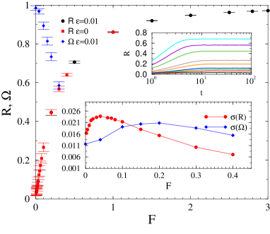
Figure 1: Order parameter dependence on $F$ for the fruit-fly connectome for the noisy (black bullet) and the noiseless (red boxes) cases at $K=1.3$. The blue diamonds show the steady-state $\Omega$ values with noise. Lower inset: Variances of $R$ and $\Omega$ for the noisy case. Upper inset: Time dependence of the noisy $R(t)$, for $F=$ 0, 0.02, 0.03, 0.04, 0.07, 0.1, 0.2, 0.3, 0.4 (bottom to top curves).

Results with and without a small noise with amplitude $\epsilon=0.01$ did not show observable differences, so the chaotic noise from the quenched disorder is capable to compete with the ordering effect of the force.

As the next step we performed the same analysis of the human connectomes at $K=1$, which is in the asynchronous phase without a force  Ódor and Kelling (2019). Figure 2 shows the steady state values both for $R$ and $\Omega$ in case of $K=1$ for KKI-113. Again the annealed noise does not modify the results and seems to be unnecessary to produce a synchronization transition. We estimated: $F^{\prime}_{c}\simeq 0.4$ and $F_{c}\simeq 0.55$ by the half values or $R$ and $\Omega$ respectively. The fluctuation peaks of the two order parameters are again far away from each other: $F^{\prime}\simeq 0.05$ versus $F\simeq 0.4$. Again the fluctuation peak of $\Omega$ is close to $F^{\prime}_{c}\simeq 0.4$.

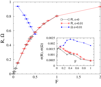
Figure 2: Order parameter dependence on $F$ for the KKI-113 for the noisy and the noiseless cases at $K=1$. Inset: Variances of $R$ and $\Omega$ for the noisy case.

For the connectome KKI-18 we enlarged the fluctuation peak results on Figure 3. The smeared synchronization ’peaks’ happen at similar values as for KKI-113: $F^{\prime}\simeq 0.05$ and $F\simeq 0.5$ within numerical precision. The transition points, estimated by the half values of $R$ is $F^{\prime}c\simeq 0.4$ and of $\Omega$ is $F_{c}\simeq 0.55$. Again, the $\sigma(R)$ peaks are much lower than the other transition point estimates.

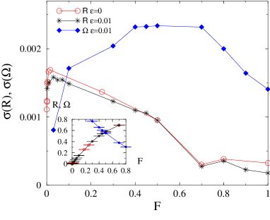
Figure 3: Fluctuations of $R$ and $\Omega$ as the function of $F$ for the KKI-18, for the noisy and the noiseless cases at $K=1$. Inset: Order parameters for the noisy and noiseless cases..

III.2 Avalanche durations

We investigated avalanches similarly to the local field potential experiments and as it was done in simulations of spike-like events Buendía et al. (2021). However, we did not threshold individual variables $\theta(t)_{i}$, but the global order parameter $R(t)$, which is a sum of them. This has the advantage of a much faster algorithm, allowing to consider larger statistics and the lack of ambiguity in avalanche definitions  Touboul and Destexhe (2010); Villegas et al. (2019); Dalla Porta and Copelli (2019). The disadvantage is that spatially independent avalanches overlapping in time accidentally may be unified, thus the duration times can be larger and we do not have information on the spatio-temporal sizes, thus on the exponent $\tau$. Still, we think that investigating this coarse-grained description of avalanches, which has also been measured in experiments, as a kind of crackling noise Sethna et al. (2001) in the case of zebrafish larvae Ponce-Alvarez et al. (2018), describes a possible critical behavior. Results of local characterization of the synchronization will be shown in Sects. 8, III.4, IV.2.

As in Buendía et al. (2021) here we also found that the choice of threshold $T(F)$ value did not change the scaling behavior of the duration distributions if it was chosen within the fluctuation range $R_{\mathrm{min}}<T(F)<R_{\mathrm{max}}$ corresponding to $F$, that was determined numerically after several runs on different initial conditions. For thresholds we used the mean value of $R(t)$, obtained in the steady state by sample and time averaging up to $t_{max}=10^{4}$. By the integration we used uniform random distributions $\theta_{i}(0)\in(0,2\pi)$ and the initial frequencies were set to be $\dot{\theta_{i}}(0)=\omega_{i}^{0}$. Following measurements of the avalanche duration $\Delta(t)=t_{i}-t_{i^{\prime}}$, defined between subsequent crossing of an up event: $R(t_{i})>T$ and a down one: $R(t_{i}^{\prime})<T$, we applied a histogramming to determine the probability distributions $p(\Delta(t))$.

Fig. 4 shows the pdf-s $p(\Delta(t))$ results for the fruit-fly in case of $K=1.3$, $\epsilon=0.01$ and different forces. We can see $F$ dependent extended PL tails, with continuously changing exponents: $2.1<\alpha<2.8$, which are somewhat smaller, but close to the experimental values for the zebrafish: $\alpha=3.0(1)$ Ponce-Alvarez et al. (2018).

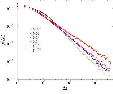
Figure 4: Avalanche duration distributions on the fruit-fly connectome for different forces, shown by the legends and at $K=1.3$, $\epsilon=0.01$. Dashed lines are PL fits for $\Delta t>100$.

Similar results are obtained in case of the two human connectomes as shown on Figs.4,5. Furthermore, the results do not change without the additive noise, or in case of a force in the synchronized phase (see graphs in the Appendix).

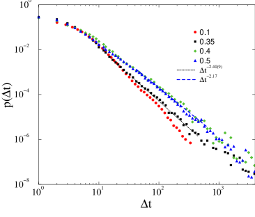
Figure 5: Avalanche duration distributions on the KKI-113 connectome for different forces, shown by the legends and at $K=1$, $\epsilon=0.01$. Dashed lines are PL fits for $\Delta t>20$.

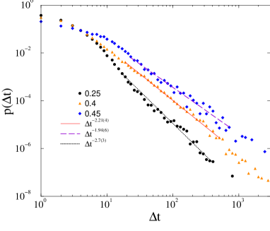
Figure 6: Avalanche duration distributions on the KKI-18 connectome for different forces, shown by the legends and at $K=1$, $\epsilon=0.01$. Dashed lines are PL fits for $\Delta t>20$.

III.3 Local order parameters snapshots

We have plotted with Wolfram Mathematica Research (2022) snapshots of the local order parameters of the FF at different force values in increasing order for the average local parameters (see Fig. 7). The giant component of the graph was plotted with $21\,615$ nodes, however with a very few $75\,657$ edges for better visualization, where we sorted the links of each node by their weights in a decreasing manner and then randomly chose the first $n_{r}$ links, where $n_{r}$ is a random integer between 1 and $n_{m}=6$. Since the graph is a modular small-world graph, this kind of representation can be a close visual representation of the actual network. The color coding on the figure is a logarithmic ($\log_{3}$) binned scale between $0$ and $1$ (0.01, 0.03, 0.09, 0.27, 0.81, 1.) representing the $R_{i}$ values of each node at time step, indicated on the top left of each figure.

Top row plots are results without force, second row at $F=0.04$, third row at $F=0.1$ and last row is at $F=1.0$. Similarly to the $\beta$ exponent’s case, we notice that the average local parameter $R$ is not increasing linearly with the force at the same time-step. There is a maximum around $0.1$, thus it does not have a linear correlation with the force. Without force the steady state has more fluctuations and the communities are more observable through visualization. By increasing the force every node comes into the same local state.

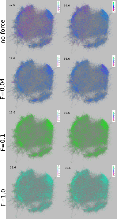
Figure 7: Here we see the evolution of the local order parameters of a sub-graph of the fruit-fly connectome at different time steps: $t=12.6,36.6$. The upper row shows $R_{i}$ map without a force, the lowest one with $F=1.0$.

III.4 Hurst and $\beta$ exponent results

The $H$ and $\beta$ exponents measure the self-similarity of a time series, when power-law behavior (10), (11) can be observed. $H$ and $\beta$ values lower than $0.5$ describe anti-correlated signals. On the other hand, values between $0.5$ and $1$ mean signals with long range correlations in time.

First, we separated the communities in all FF, KK-18, KKI-113 connectomes with the Louvain modularity optimizing algorithm. Then, we calculated the $H$ and $\beta$ exponents for each community for the local parameters. In case of the FF the results (see Fig. 8 with force could similarly be differentiated from the results without force as in the  Ochab et al. (2022) experiments with rest and task driven measures. Simulation results without force seem to have longer correlations in time, resembling to the fMRI measurements at the rest phase.

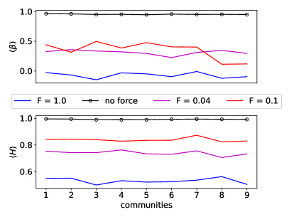
Figure 8: Hurst and beta exponents of all fruit-fly connectome communities. In the forceless case at the critical Hopf transition coupling, the $H$ exponent is the largest for every community. With forces these values drop for each community. This shows a resemblance with the rest and non-rest studies of different brain areas in Ochab et al. (2022), showing $\langle H\rangle\approx 1.0$ at resting state and $\langle H\rangle\approx 0.7$ at task driven states.

The same conclusion however cannot be found in the case of the human connectomes (see Fig. 9). It appears that even with a relatively high force the exponents remain close to each other and close to those of the “rest" phase. In the case of FF higher force led to less “rest" in the system resembling more like task driven behaviour.

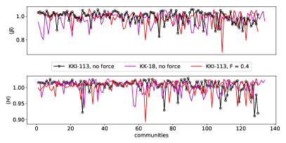
Figure 9: Hurst and $\beta$ exponents of all human connectomes’ communities. KKI-113 is presented with and without force terms and KK-18 without the force terms.

IV Hopf synchronization transition without force

We have rerun this analysis for the fruit-fly connectome using the standard Kuramoto equation for different couplings, i.e. near the Hopf synchronization transition discussed in Ódor et al. (2022).

IV.1 Crackling noise analysis

Earlier mean-field type of phase transition was found at $K_{c}\simeq 1.7(2)$. As we can see on Fig. 10 the crackling noise duration analysis results in faster than PL decays of $p(\Delta t)$ for $K<1.4$ and an inflection point with up veering decays for $K\geq 1.65$ couplings. At $K=1.5$ we can observe a PDF, with PL decay for $30<t<300$, which can be fitted by the exponent $\alpha=3.03(3)$.

As in Ódor et al. (2022) we do not find an extended scaling region with non-universal exponents suggesting a GP. So, the crackling noise exponent, presumably the mean-field class exponent of the Hopf transition, describing the resting state, should be this value. This is a rather large exponent and is difficult to reproduce by simulations, because large systems are needed to see the scaling region before an exponential cutoff. We assume that this was not seen in Buendía et al. (2021), where $N=500$ nodes were used. Another reason might be that in Buendía et al. (2021) an annealed Kuramoto model was simulated, lacking the quenched self-frequencies. Or perhaps because Buendía et al. (2021) used thresholds of the $\theta_{i}(t)$ variables and identified avalanches by estimating the spatio-temporal size of the activity avalanches.

But indeed the scaling region we observe is rathernarrow, even though we know that the Kuramoto model exhibits a critical synchronization transition here.

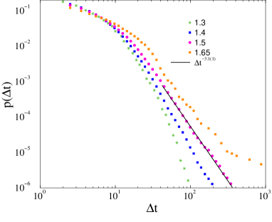
Figure 10: Avalanche duration distributions on the fruit-fly connectome without force for $K$ different couplings.

IV.2 Hurst and $\beta$ analysis of local variables

We cannot exclude the possibility that doing the avalanche analysis on the local angles $\theta_{i}(t)$, would lead to a lack of PL-s as it was claimed in  Buendía et al. (2021). Since identification of avalanches of local variables is a rather difficult and ambiguous task, requiring careful binning, to check the scaling of local phase and frequency data we performed auto-correlation measurements and estimated the Hurst and $\beta$ exponents as before.

The "no-force" result on Figs. 8 and  9 show strong auto-correlations, indications of criticality as in the brain experiments  Ochab et al. (2022). In fact the exponents are larger (close to 1), than in case of the Shinomoto–Kuramoto model calculations. This suggests that the external excitation results in a less correlated scaling behavior of the neural systems than in the resting state. These results are in agreement with the experimental findings of  Ochab et al. (2022).

V Conclusions

In conclusion our numerical analysis of synchronization models on different connectome graphs show that in the case of excitation we can find PL scaling of duration of the crackling noise of the activity, defined by thresholds of $R$. By solving the Shinomoto-Kuramoto model numerically we concluded that even without the additive noise we can find similar synchronization transition as with the full Langevin equation.

The observed PL tails exhibit some dependence on the amplitude of the force, which may be related to GP heterogeneity effects, but can also arise as the consequence of quasi-critical, scaling like behavior reported in the discrete models of Ref. Fosque et al. (2021). We estimated the extension of the synchronization transition region by the fluctuations of $R$ and $\Omega$ and found an extended, smeared transition region. This makes it difficult to define the transition points. We attempted it in two different ways: half values and fluctuation peaks of the order parameters in the steady state. The $F^{\prime}_{c}$ from the $R$ half values are somewhat smaller than the $F_{c}$ of $\Omega$-s and agree with the frequency fluctuation peaks. While the phase fluctuations peaks were found to be much smaller both for the FF and the human connectomes. This is very different from the Kuramoto Hopf transition results Ódor et al. (2022).

However, $\sigma(R)$ describes a transition of the SK order parameter, introduced for excitable systems. In the case of the synchronized transition in FF the addition of force results in a quick decay of the SK order parameter like in the SNIC transition. We have not reached a region, showing hybrid phase transition reported in Buendía et al. (2021), possibly by the lack of strong noise. We avoided to apply strong noise, because that makes the numerical solution less precise or very slow. A systematic finite-size scaling study of this transition would be necessary to settle this issue.

In case of initial conditions with random phase variables the $R(t)$ curves at the transition point do not show PL growth as in case of the Kuramoto model, but a logarithmic growth, similar to strong random fixed points of models of statistical physics.

We also investigated the local order parameters and found frustrated synchronization with Chimera like states, coexistence of synchronized and asynchronous domains. Performing auto-correlation analysis on the local order parameters we found strong auto-correlation in the resting (Kuramoto) state at criticality and somewhat weaker ones in presence of an external force. In the latter case the $H$ and $\beta$ exponents take their maximal values, where the fluctuations of $R(t)$ are maximal, i.e at the transition.

We also investigated the module dependence of $H$ and $\beta$ by decomposing the connectomes via community detection algorithms. We observed variations amongst the communities suggesting different levels of criticality, but the identification of communities with real brain regions is a further task to be completed. Our simulated $H$ and $\beta$ exponents are in agreement with recent experimental findings Ochab et al. (2022).

Appendix

Here we show avalanche duration PDF-s without noise in case of the KKI-113 connectome on Fig. 11. One see only a slight variation of the PL tail exponents around $-2.2$, but they are close to the noisy case results.

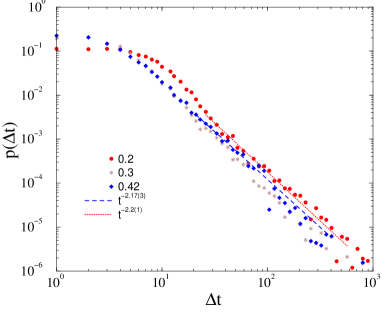
Figure 11: Avalanche duration distributions on the KKI-113 connectome for different forces, shown by the legends and at $K=1$, without noise. Dashed lines are PL fits for $\Delta t>20$.

Similarly, in case of the FF with the application of force in the synchronized phase, i.e. $K=2$ the PL tails fitted for $t>20$ do not differ to much, they can be characterized by an exponent $-2.21(1)$ as one can see on Fig. 12. The inset shows the rapid drop of the SK order parameter as the function of the force and the maximum both of $\sigma(R)$, $\sigma(\Omega)$ are at $F\simeq 0$

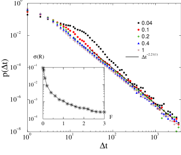
Figure 12: Avalanche duration distributions on the fruit-fly connectome for different forces, shown by the legends and at $K=2$, $\epsilon=0.01$. Dashed lines are PL fits for $\Delta t>100$. The inset shows $\sigma(R)$ by increasing $F$.

References

- Beggs and Plenz (2003) J. Beggs and D. Plenz, J. Neuroscience 23, 11167 (2003).
- Mazzoni et al. (2007) A. Mazzoni, F. D. Broccard, E. Garcia-Perez, P. Bonifazi, M. E. Ruaro, and V. Torre, PLOS ONE 2, 1 (2007).
- Pasquale et al. (2008) V. Pasquale, P. Massobrio, L. Bologna, M. Chiappalone, and S. Martinoia, Neuroscience 153, 1354 (2008).
- Friedman et al. (2012) N. Friedman, S. Ito, B. A. W. Brinkman, M. Shimono, R. E. L. DeVille, K. A. Dahmen, J. M. Beggs, and T. C. Butler, Phys. Rev. Lett. 108, 208102 (2012).
- Hahn et al. (2010) G. Hahn, T. Petermann, M. N. Havenith, S. Yu, W. Singer, D. Plenz, and D. Nikolić, Journal of Neurophysiology 104, 3312 (2010), pMID: 20631221.
- Shriki et al. (2013) O. Shriki, J. Alstott, F. Carver, T. Holroyd, R. N. Henson, M. L. Smith, R. Coppola, E. Bullmore, and D. Plenz, Journal of Neuroscience 33, 7079 (2013).
- Tagliazucchi et al. (2012) E. Tagliazucchi, P. Balenzuela, D. Fraiman, and D. Chialvo, Frontiers in Physiology 3, 15 (2012).
- Scott et al. (2014) G. Scott, E. D. Fagerholm, H. Mutoh, R. Leech, D. J. Sharp, W. L. Shew, and T. Knöpfel, Journal of Neuroscience 34, 16611 (2014).
- Priesemann et al. (2014) V. Priesemann, M. Wibral, M. Valderrama, R. Pröpper, M. Le Van Quyen, T. Geisel, J. Triesch, D. Nikolić, and M. H. J. Munk, Frontiers in Systems Neuroscience 8, 108 (2014).
- Bellay et al. (2015) T. Bellay, A. Klaus, S. Seshadri, and D. Plenz, Elife 4, e07224 (2015).
- Hahn et al. (2017) G. Hahn, A. Ponce-Alvarez, C. Monier, G. Benvenuti, A. Kumar, F. Chavane, G. Deco, and Y. Frégnac, PLOS Computational Biology 13, 1 (2017).
- Seshadri et al. (2018) S. Seshadri, A. Klaus, D. Winkowski, and et al., Transl Psychiatry 8 (2018).
- Palva et al. (2013) J. Palva, A. Zhigalov, J. Hirvonen, O. Korhonen, K. Linkenkaer-Hansen, and S. Palva, Proceedings of the National Academy of Sciences of the United States of America 110, 3585 (2013).
- Fuscà et al. (2022) M. Fuscà, F. Siebenhühner, S. H. Wang, V. Myrov, G. Arnulfo, L. Nobili, J. M. Palva, and S. Palva, bioRxiv (2022).
- Ponce-Alvarez et al. (2018) A. Ponce-Alvarez, A. Jouary, M. Privat, G. Deco, and G. Sumbre, Neuron 100, 1446 (2018).
- Yaghoubi et al. (2018) M. Yaghoubi, T. De Graaf, J. Orlandi, F. Girotto, M. Colicos, and J. Davidsen, Scientific Reports 8 (2018).
- Chialvo and Bak (1999) D. Chialvo and P. Bak, Neuroscience 90, 1137 (1999).
- Chialvo (2004) D. R. Chialvo, Physica A: Statistical Mechanics and its Applications 340, 756 (2004), complexity and Criticality: in memory of Per Bak (1947–2002).
- Chialvo (2006) D. R. Chialvo, Nature Physics 2, 301 (2006).
- Chialvo (2007) D. R. Chialvo, AIP Conference Proceedings 887, 1 (2007), eprint https://aip.scitation.org/doi/pdf/10.1063/1.2709580.
- Chialvo et al. (2008) D. R. Chialvo, P. Balenzuela, and D. Fraiman, AIP Conference Proceedings 1028, 28 (2008), eprint https://aip.scitation.org/doi/pdf/10.1063/1.2965095.
- Fraiman et al. (2009) D. Fraiman, P. Balenzuela, J. Foss, and D. R. Chialvo, Phys. Rev. E 79, 061922 (2009).
- Expert et al. (2011) P. Expert, R. Lambiotte, D. R. Chialvo, K. Christensen, H. J. Jensen, D. J. Sharp, and F. Turkheimer, Journal of The Royal Society Interface 8, 472 (2011).
- Fraiman and Chialvo (2012) D. Fraiman and D. Chialvo, Frontiers in Physiology 3, 307 (2012).
- Deco and Jirsa (2012) G. Deco and V. K. Jirsa, Journal of Neuroscience 32, 3366 (2012).
- Deco et al. (2014) G. Deco, A. Ponce-Alvarez, P. Hagmann, G. Romani, D. Mantini, and M. Corbetta, Journal of Neuroscience 34, 7886 (2014).
- Senden et al. (2017) M. Senden, N. Reuter, M. P. van den Heuvel, R. Goebel, and G. Deco, NeuroImage 146, 561 (2017).
- Muñoz (2018) M. A. Muñoz, Rev. Mod. Phys. 90, 031001 (2018).
- Plenz et al. (2021) D. Plenz, T. L. Ribeiro, S. R. Miller, P. A. Kells, A. Vakili, and E. L. Capek, Frontiers in Physics 9, 365 (2021).
- Kinouchi and Copelli (2006) O. Kinouchi and M. Copelli, Nature Physics 2, 348 (2006).
- Bak et al. (1987) P. Bak, C. Tang, and K. Wiesenfeld, Phys. Rev. Lett. 59, 381 (1987).
- Vojta (2006) T. Vojta, Journal of Physics A: Mathematical and General 39, R143 (2006).
- Ódor et al. (2021) G. Ódor, M. T. Gastner, J. Kelling, and G. Deco, Journal of Physics: Complexity 2, 045002 (2021).
- Fosque et al. (2021) L. J. Fosque, R. V. Williams-García, J. M. Beggs, and G. Ortiz, Phys. Rev. Lett. 126, 098101 (2021).
- Korchinski et al. (2021) D. J. Korchinski, J. G. Orlandi, S.-W. Son, and J. Davidsen, Phys. Rev. X 11, 021059 (2021), URL https://link.aps.org/doi/10.1103/PhysRevX.11.021059.
- Almeira et al. (2022) J. Almeira, T. S. Grigera, D. R. Chialvo, and S. A. Cannas, Phys. Rev. E 106, 054140 (2022), URL https://link.aps.org/doi/10.1103/PhysRevE.106.054140.
- Ódor and de Simoni (2021) G. Ódor and B. de Simoni, Phys. Rev. Research 3, 013106 (2021).
- Corral López et al. (2022) R. Corral López, V. Buendía, and M. A. Muñoz, Phys. Rev. Research 4, L042027 (2022), URL https://link.aps.org/doi/10.1103/PhysRevResearch.4.L042027.
- Buendía et al. (2021) V. Buendía, P. Villegas, R. Burioni, and M. A. Muñoz, Phys. Rev. Research 3, 023224 (2021), URL https://link.aps.org/doi/10.1103/PhysRevResearch.3.023224.
- Morales et al. (2022) G. B. Morales, S. Di Santo, and M. A. Muñoz, bioRxiv (2022).
- Ye and Vojta (2022) X. Ye and T. Vojta, Phys. Rev. E 106, 044102 (2022), URL https://link.aps.org/doi/10.1103/PhysRevE.106.044102.
- Ódor (2019) G. Ódor, Physical Review E 99, 012113 (2019).
- Griffiths (1969) R. B. Griffiths, Phys. Rev. Lett. 23, 17 (1969).
- Moretti and Muñoz (2013) P. Moretti and M. A. Muñoz, Nature Communications 4, 2521 (2013).
- Ódor et al. (2015) G. Ódor, R. Dickman, and G. Ódor, Scientific Reports 5, 14451 (2015).
- Cota et al. (2018) W. Cota, G. Ódor, and S. C. Ferreira, Scientific Reports 8, 9144 (2018).
- Buendí a et al. (2022) V. Buendí a, P. Villegas, R. Burioni, and M. A. Muñoz, Philosophical Transactions of the Royal Society A: Mathematical, Physical and Engineering Sciences 380 (2022), URL https://doi.org/10.1098%2Frsta.2020.0424.
- Cota et al. (2016) W. Cota, S. C. Ferreira, and G. Ódor, Phys. Rev. E 93, 032322 (2016).
- Burkitt (2006) A. N. Burkitt, Biological Cybernetics 95, 1 (2006), ISSN 1432-0770, URL https://doi.org/10.1007/s00422-006-0068-6.
- Liang et al. (2020) J. Liang, T. Zhou, and C. Zhou, Frontiers in Systems Neuroscience 14 (2020), ISSN 1662-5137.
- Orlandi et al. (2013) J. G. Orlandi, J. Soriano, E. Alvarez-Lacalle, S. Teller, and J. Casademunt, Nature Physics 9, 582 (2013).
- Janssen (1981) H. K. Janssen, Z. Phys. B 42, 151 (1981).
- Grassberger (1982) P. Grassberger, Z. Phys. B 47, 365 (1982).
- Ódor (2008) G. Ódor, Universality in nonequilibrium lattice systems: Theoretical foundations (World Scientific, 2008).
- Ódor (2016) G. Ódor, Phys. Rev. E 94, 062411 (2016).
- Ódor and Kelling (2019) G. Ódor and J. Kelling, Scientific Reports 9, 19621 (2019).
- Ódor et al. (2021) G. Ódor, J. Kelling, and G. Deco, J. Neurocomputing 461, 696 (2021).
- Ódor et al. (2022) G. Ódor, G. Deco, and J. Kelling, Phys. Rev. Research 4, 023057 (2022), URL https://link.aps.org/doi/10.1103/PhysRevResearch.4.023057.
- Villegas et al. (2014) P. Villegas, P. Moretti, and M. Muñoz, Scientific Reports 4 (2014).
- Villegas et al. (2016) P. Villegas, J. Hidalgo, P. Moretti, and M. Muñoz (2016), pp. 69–80.
- Millán et al. (2018) A. Millán, J. Torres, and G. Bianconi, Scientific Reports 8 (2018).
- Ochab et al. (2022) J. K. Ochab, M. Wątorek, A. Ceglarek, M. Fafrowicz, K. Lewandowska, T. Marek, B. Sikora-Wachowicz, and P. Oświęcimka, Scientific Reports 12, 17866 (2022), ISSN 2045-2322, URL https://doi.org/10.1038/s41598-022-21375-1.
- Kuramoto (2012) Y. Kuramoto, Chemical Oscillations, Waves, and Turbulence, Springer Series in Synergetics (Springer Berlin Heidelberg, 2012), ISBN 9783642696893.
- Shinomoto and Kuramoto (1986) S. Shinomoto and Y. Kuramoto, Progress of Theoretical Physics 75, 1105 (1986), ISSN 0033-068X.
- Sakaguchi (1988) H. Sakaguchi, Progress of Theoretical Physics 79, 39 (1988).
- Antonsen et al. (2008) T. M. Antonsen, R. T. Faghih, M. Girvan, E. Ott, and J. Platig, Chaos: An Interdisciplinary Journal of Nonlinear Science 18, 037112 (2008).
- Ott and Antonsen (2008) E. Ott and T. M. Antonsen, Chaos: An Interdisciplinary Journal of Nonlinear Science 18, 037113 (2008).
- Childs and Strogatz (2008) L. M. Childs and S. H. Strogatz, Chaos: An Interdisciplinary Journal of Nonlinear Science 18, 043128 (2008).
- P. (1983) D. P., Numerische Mathematik 41, 399 (1983).
- Hairer et al. (1987) E. Hairer, S. P. Norsett, and G. Wanner, Solving Ordinary Differential Equations I. Nonstiff Problems., vol. 8 of Springer Series in Comput. Mathematics (Springer-Verlag, 1987), 2nd ed.
- Maruyama (1955) G. Maruyama, Rendiconti del Circolo Matematico di Palermo 4, 48 (1955), ISSN 1973-4409, URL https://doi.org/10.1007/BF02846028.
- Lima Dias Pinto and Copelli (2019) I. Lima Dias Pinto and M. Copelli, Phys. Rev. E 100, 062416 (2019).
- Sporns et al. (2005) O. Sporns, G. Tononi, and R. Kötter, PLOS Computational Biology 1, e42 (2005).
- dow (2020) The hemibrain dataset (v1.0.1) (2020), URL https://storage.cloud.google.com/hemibrain-release/neuprint/hemibrain_v1.0.1_neo4j_inputs.zip.
- Landman et al. (2011) B. A. Landman, A. J. Huang, A. Gifford, D. S. Vikram, I. A. L. Lim, J. A. D. Farrell, J. A. Bogovic, J. Hua, M. Chen, S. Jarso, et al., NeuroImage 54, 2854 (2011).
- Delettre et al. (2019) C. Delettre, A. Messé, L.-A. Dell, O. Foubet, K. Heuer, B. Larrat, S. Meriaux, J.-F. Mangin, I. Reillo, C. de Juan Romero, et al., Network Neuroscience 3, 1038 (2019).
- Gastner and Ódor (2016) M. T. Gastner and G. Ódor, Scientific Reports 6, 27249 (2016).
- OCP (2015) Neurodata, https://neurodata.io (2015).
- Gray Roncal et al. (2013) W. Gray Roncal, Z. H. Koterba, D. Mhembere, D. M. Kleissas, J. T. Vogelstein, R. Burns, A. R. Bowles, D. K. Donavos, S. Ryman, R. E. Jung, et al., in 2013 IEEE Global Conference on Signal and Information Processing (2013), pp. 313–316.
- (80) neurodata / m2g.
- Desikan et al. (2006) R. S. Desikan, F. Ségonne, B. Fischl, B. T. Quinn, B. C. Dickerson, D. Blacker, R. L. Buckner, A. M. Dale, R. P. Maguire, B. T. Hyman, et al., NeuroImage 31, 968 (2006).
- Klein and Tourville (2012) A. Klein and J. Tourville, Frontiers in Neuroscience 6, 171 (2012).
- Newman (2006) M. E. J. Newman, Proc Natl Acad Sci U S A 103, 8577 (2006).
- Blondel et al. (2008) V. D. Blondel, J.-L. Guillaume, R. Lambiotte, and E. Lefebvre, Journal of Statistical Mechanics: Theory and Experiment 2008, P10008 (2008).
- Humphries and Gurney (2008) M. D. Humphries and K. Gurney, PLOS ONE 3, e0002051 (2008).
- Restrepo et al. (2005) J. G. Restrepo, E. Ott, and B. R. Hunt, Physical Review E 71, 036151 (2005).
- Schröder et al. (2017) M. Schröder, M. Timme, and D. Witthaut, Chaos: An Interdisciplinary Journal of Nonlinear Science 27, 073119 (2017).
- Sanchez-Rodriguez et al. (2021) L. M. Sanchez-Rodriguez, Y. Iturria-Medina, P. Mouches, and R. C. Sotero, NeuroImage 225, 117431 (2021), ISSN 1053-8119, URL https://www.sciencedirect.com/science/article/pii/S1053811920309162.
- Deritei et al. (2014) D. Deritei, Z. I. Lázár, I. Papp, F. Járai-Szabó, R. Sumi, L. Varga, E. R. Regan, and M. Ercsey-Ravasz, New Journal of Physics 16, 063007 (2014), URL https://dx.doi.org/10.1088/1367-2630/16/6/063007.
- Lázár et al. (2017) Z. I. Lázár, I. Papp, L. Varga, F. Járai-Szabó, D. Deritei, and M. Ercsey-Ravasz, Phys. Rev. E 95, 022306 (2017), URL https://link.aps.org/doi/10.1103/PhysRevE.95.022306.
- Touboul and Destexhe (2010) J. Touboul and A. Destexhe, PloS one 5, e8982 (2010).
- Villegas et al. (2019) P. Villegas, S. Di Santo, R. Burioni, and M. A. Muñoz, Physical Review E 100, 012133 (2019).
- Dalla Porta and Copelli (2019) L. Dalla Porta and M. Copelli, PLoS computational biology 15, e1006924 (2019).
- Sethna et al. (2001) J. P. Sethna, K. A. Dahmen, and C. R. Myers, Nature 410, 242 (2001).
- Research (2022) W. Research, Graph, https://reference.wolfram.com/language/ref/Graph.html (2022).