Modeling adaptive forward-looking behavior in epidemics on networks

Abstract

The course of an epidemic can be drastically altered by changes in human behavior. Incorporating the dynamics of individual decision-making during an outbreak represents a key challenge of epidemiology, faced by several modeling approaches siloed by different disciplines. Here, we propose an epi-economic model including adaptive, forward-looking behavioral response on a heterogeneous networked substrate, where individuals tune their social activity based on future health expectations. Under basic assumptions, we show that it is possible to derive an analytical expression of the optimal value of the social activity that matches the traditional assumptions of classic epidemic models. Through numerical simulations, we contrast the settings of global awareness – individuals only know the prevalence of the disease in the population – with local awareness, where individuals explicitly know which of their contacts are infected. We show that behavior change can flatten the epidemic curve by lowering the peak prevalence, but local awareness is much more effective in curbing the disease early with respect to global awareness. Our work bridges classical epidemic modeling with the epi-economic approach, and sheds light on the effects of heterogeneous behavioral responses in curbing the epidemic spread.

1 Introduction

Behavioral adaptation in response to infectious disease outbreaks is one of the key factors that shape the course of an epidemic [1]. Individual choices regarding the adoption of self-protective measures, such as wearing masks, avoiding close social contacts, or vaccinating, contribute to reducing disease transmission in the population. In turn, such choices depend on the perceived severity of the epidemic, the available information about it, and individual risk perception, thus they vary over time as the epidemic progresses. As the epidemic fades out, behavioral responses may relax, with the consequence of leading to disease resurgence. Self-initiated behavioral responses have been observed across all kinds of epidemics, from small-scale outbreaks, involving few individuals, such as the 2015 Middle East respiratory syndrome outbreak in South Korea [2], to worldwide pandemics, such as the 1918 pandemic [3], the 2009 A/H1N1 pandemic [4, 5, 6], as well as the current COVID-19 pandemic [7].

Incorporating the dynamics of individual decision-making during an outbreak represents a key challenge of epidemic modeling [8]. To this aim, a wide variety of mathematical epidemic models that capture the effects of behavioral changes have been proposed [9, 10, 11]. Generally speaking, these models can be classified into three broad classes. In the simplest case, classical compartmental models have been expanded to consider additional behavioral classes in the population, characterized by different behavioral responses to the disease prevalence, whose transmission parameters do not change over time [12, 13]. The second class of models includes those that aim at capturing the interplay between individual adaptation and individual knowledge of the disease, often represented as two coupled dynamical processes [14, 15]. Information about the disease can be local or global, and sometimes it is assumed to spread through the population [16]. Finally, a distinct class of models aims to explicitly describe the individual decision-making process using approaches of behavioral economics, where individuals evaluate their payoffs and adopt the behavior that optimally increases the payoff [17, 18]. These “epi-economic" models simulate the process by which people choose the best course of action by adjusting to the current epidemic state and seeking the best possible future outcome via an optimization process [19, 20, 21, 22]. Such optimization processes typically rely on numerical methods.

The COVID-19 pandemic reopened the debate on how human behavior should be included in epidemic models, with researchers with many different backgrounds contributing to the modeling effort, including for instance game-theoretical models [23, 24]. However, different approaches have often been siloed within the boundaries of the related discipline and consequent limitations. On the one hand, agent-based models with additional behavioral classes require a behavioral response to be defined a-priori. On the other hand, epi-economic models do consider an adaptive response but generally rely on the homogeneous mixing hypothesis, under which all susceptible individuals have an equal chance of contracting the infection. The great degree of heterogeneity in human behavior [25, 26, 27, 28] makes it clear that different individuals have varying chances of contracting the disease. As a consequence, heterogeneous behavioral responses in the population should arise also under the epi-economic approach.

In this work, we try to fill this gap by proposing an epi-economic model including adaptive, forward-looking behavioral response on a heterogeneous networked substrate. Individuals choose their social activity to maximize their future expected utility, by balancing the risk of being infected in the future while maintaining the highest possible social activity. We rely on some simplifying yet realistic assumptions that allow us to describe the optimal behavior by an analytical expression depending on the epidemic conditions (prevalence and disease parameters) and the behavior of the population itself. We explicitly contrast the cases of global awareness, in which individuals have a bird-eye view of the epidemic unfolding on the whole population, with a local awareness setting, where individuals only know which of their contacts are infected. The latter case triggers a highly heterogeneous behavioral response. We show that behavior change can flatten the epidemic curve by lowering the peak prevalence, thus potentially reducing the load on the health system at the epidemic peak. However, local awareness is much more effective in curbing early the disease with respect to global awareness, thus shrinking the overall number of infections.

2 Results

2.1 A model of forward-looking adaptive behavior

We propose an analytically tractable epidemic model including a feedback loop between the social activity of individuals and the spreading of the epidemic. To this aim, we consider a SIR model in which individuals change their behavior, reducing or increasing their social activity, depending on the prevalence of the disease. Crucially, susceptible individuals tune their social activity with a forward-looking approach, i.e., they balance the risk of being infected in the future while maintaining the highest possible social activity.

The base of our model will be the SIR model [29] in discrete time steps. We consider a population of $N$ individuals, each one belonging to one of three compartments: susceptible ($S$), infected ($I$), or recovered ($R$). A $S$ individual who is in contact with a $I$ individual has a probability $\beta$ of becoming infected in a day. Each $I$ individual has a probability $\mu$ of recovering. $R$ individuals can not be infected anymore.

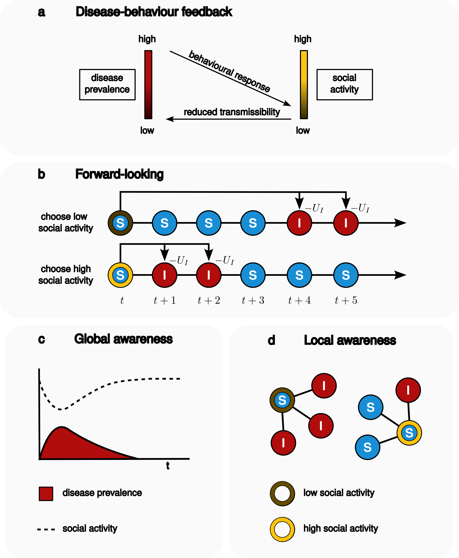
Next, we specify how changing behavior affects the probability of infection. Inspired by Ref. [21], we define a time-dependent social activity $a_{t}$ for individuals, representing their propensity of engaging in social interactions with peers. Social activity is bounded ${0\leq a_{t}\leq 1}$, with ${a=1}$ corresponding to normal behavior in absence of the disease, and ${a=0}$ corresponding to a situation in which disease transmission is not possible, equivalent to quarantine. We assume that disease transmission between individuals depends on their social activity. If a $S$ individual with social activity $a_{t}^{S}$ comes into contact at time $t$ with an $I$ individual with social activity $a_{t}^{I}$, we assume the probability of the $S$ individual getting infected to depend linearly on both $a_{t}^{S}$ and $a_{t}^{I}$, so that the $S$ individual gets infected with probability ${\beta a_{t}^{S}a_{t}^{I}}$. We note that the social activity $a_{t}$ can have multiple interpretations as long as they result in a decreased probability of disease transmission. For instance, a lower social activity could represent less frequent contacts with other individuals or it could represent the adoption of prophylactic measures, such as the use of face masks in the case of airborne disease ([30]), that limit the probability of infection on contact without actually reducing the contact rate. Intuitively, individuals limit their social activity in order to reduce the probability to be infected: when the prevalence is high, they will adopt prudent behavior. The feedback loop between the disease spread and social activity is illustrated in Figure 1 (a).

Following the epi-economic approach, we model the dynamics of $a_{t}$ as an optimization process in which $S$ individuals balance the risk of infection and the benefits of social activity, which are represented by a utility function. At each time step, each individual is assigned a score, named utility, based on their behavior and health status. Adopting a behavior that reduces the probability of infection (i.e. lower social activity) results in lower utility, but also reduces the probability of getting infected which would also result in a penalty. At each time step, each individual deals with this trade-off by choosing the behavior that maximizes its future expected utility (objective function), see Fig. 1 (b). A common strategy to approach this problem is dynamic programming, which can be solved via the Bellman Equation [19, 31, 32]. Here, we make a series of simplifying assumptions that allow us to find an analytical expression for the optimal value of the social activity.

Figure 1: Schematic illustration of the model. (a) Feedback loop involving epidemic spreading and social activity. If the prevalence is high, individuals can decrease their social activity, which in turn reduces the transmissibility of the disease, decreasing prevalence. With low prevalence, individuals can choose high levels of social activity, increasing the prevalence. (b) Individuals choose their social activity to maximize their future expected utility. They can choose a low value of social activity to delay the expected infection (and the expected penalty $U_{I}$), or benefit from high social activity at a higher infection risk. Awareness and behavioral response can be of two kinds. Global awareness (c): individuals know the prevalence of the disease in the population but do not know who is infected, so social activity is homogeneous across the population. Local awareness (d): individuals know which of their contacts are infected, resulting in different values of social activity for each individual.

Our first simplifying assumption is that all individuals optimize social activity in the same way. This is equivalent to assuming that individuals ignore their health status. We stress that this does not necessarily mean that all individuals behave in the same way. For instance, prophylactic measures that are taken by $I$ individuals regardless of the current state of the epidemic (i.e. behavior that is not adaptive), such as always wearing a face mask when in public or reducing their contact by a fixed amount by not going to work, can be modeled by changing the value of $\beta$. Also, the behavior of $R$ individuals does not affect the dynamics of the disease in our model. Second, we assume individuals to believe that current conditions (i.e. the sizes of the $S$, $I$, and $R$ compartments, as well as their social activity $a_{t}$ and that of the rest of the population) will remain unchanged. The validity of these assumptions is discussed in Section 2.4 (Model calibration).

2.2 Utility function

We assume the utility function to be the sum of two terms $U_{a}$ and $U_{H}$: the first one depends only on social activity and the second one depends only on the health status ${H=\{S,I,R\}}$. We choose the state-dependent term $U_{H}$ of the utility function to correspond to a fixed penalty of magnitude $U_{I}$ for each time step in the infected state and to be ${U_{H}=0}$ otherwise (${H\neq I}$):

$$U_{H}(t)=\begin{cases}-U_{I}&(\text{if }H=I\text{ at time t})\\ 0&(\text{otherwise}).\end{cases}$$ (1)

To determine the functional form of the utility function related to social activity, $U_{a}$, we use the following argument. On the one hand, decreasing social activity should require a higher cost in terms of utility when social activity is already low, so we assume the derivative of $U_{a}$ with respect to $a$ to be inversely proportional to $a$. On the other hand, increasing social activity also comes with a cost, otherwise, there would be no finite optimal value of social activity (which we assumed to be $a=1$) when there is no risk of getting infected. The simplest hypothesis that we can make about this cost is that it does not depend on social activity, so we add a constant term to the derivative of $U_{a}$ with respect to $a$, resulting in $\frac{dU_{a}}{da}=\frac{A}{a}-B$, which has solution $U_{a}=A\log(a)-Ba+C$. Requiring that $a=1$ is a maximum of $U_{a}$ results in $A=B$. Since we are only interested in the position of the maximum and not in the actual value of $U_{a}$, we can fix $A=B=C=1$ without loss of generality. From which follows that at time $t$ individuals with social activity $a_{t}$ get a utility score equal to:

$$U_{a}(t)=\log(a_{t})-a_{t}+1.$$ (2)

We note that this choice of a concave form for the utility function is common in the economic literature, as well as in epi-economic models [21].

The optimal value of social activity at each time $t$ is then given by the maximum with respect to $a_{t}$ of the following objective function:

$$J(t)=\mathbb{E}\sum_{\Delta t=0}^{\infty}\ \delta^{\Delta t}\left[U_{a}(t+\Delta t)+U_{H}(t+\Delta t)\right].$$ (3)

The objective function in Eq. (3) represents the expected value, over all possible future health states, starting from the $S$ state at time $t$, of the utility function, in which utility corresponding to $\Delta t$ days into the future gets discounted by a factor ${\delta^{\Delta t}}$, where $\delta$ is the discount factor. The discount factor ${0<\delta<1}$ implies that behavior resulting in high values of utility in the near future is preferred to behavior that pays off in the distant future. It also ensures that the series in Eq. (3) converges.

Under our assumptions, it is possible to express the objective function at time $t$, Eq. (3), associated with a choice of social activity $a_{t}$ in a closed-form, see Methods:

$$J(t)=\frac{1}{1-\delta}\left[U_{a}(t)-\alpha\delta P_{I}(t)\right],$$ (4)

where the first term represents the benefits of social activity and the second term represents the risk of getting infected. The strength of the behavioral response to the infection risk is determined by the probability of becoming infected at time $t$, $P_{I}(t)$, the discount factor $\delta$, and the average utility loss caused by an infection, $\alpha$. The larger the average infection cost $\alpha$, the infection probability $P_{I}$, or the discount factor $\delta$, the stronger the behavioral response. The probability of infection depends on the choice of the underlying network substrate, and it will be discussed in the next Section. The parameter $\alpha$ instead can be calculated (see Methods) as

$$\alpha=\frac{U_{I}}{1-\delta(1-\mu)}.$$ (5)

The average cost of infection is proportional to the penalty $U_{I}$ and it becomes smaller for increasing discount factor $\delta$ (the duration of the infection is discounted by $\delta$) and the recovery rate $\mu$ (the larger $\mu$, the shorter the duration of the infection).

The optimal value of the social activity can be determined as the maximum with respect to $a$ of the objective function in Eq. (4). In particular, if the behavioral component of the utility function is given by Eq. (2), then the optimal value of social activity at time $t$ is:

$$a^{*}_{t}=\frac{1}{1+\alpha\delta\frac{\partial P_{I}(t)}{\partial a^{*}_{t}}}.$$ (6)

Therefore, individuals will adopt the optimal value of social activity $a^{*}_{t}$ at each time step $t$, depending on the constant parameters $\alpha$ and $\delta$, and on the probability of becoming infected at time $t$, $P_{I}(t)$. Note that the infection probability does depend on the underlying network’s structure and on the optimal social activity chosen by the involved individuals. From now on, we will always refer to the optimal social activity, therefore, for the sake of simplicity, we will denote it as $a_{t}$ in the remainder of the paper.

2.3 Local vs global awareness

Next, we specify the substrate over which the disease spreads. We assume that disease transmission is mediated through social interactions, represented by a contact network where nodes represent individuals and links represent contacts between them. We assume that each active link connecting a $S$ node (labelled $i$) to a $I$ neighbor (labelled $j$) can carry the disease in the unit time with probability ${\beta a_{i}a_{j}}$, where $a_{i}$ and $a_{j}$ are the social activities of the two nodes (we omit the time dependence here). By assuming independent infection processes for each active link, the probability of the $S$ node being infected by any of its $I$ neighbors is ${P_{I}=1-\prod_{j}(1-\beta a_{i}a_{j})}$, where the product runs on the infected neighbors of node $i$. If we neglect terms of order $\beta^{2}$, we obtain ${P_{I}=\beta a_{i}\sum_{j}a_{j}}$, which means that the optimal social activity (Eq. (6)) is:

$$a_{i,t+1}=\frac{1}{1+\alpha\delta\beta\sum_{j}a_{j,t}},$$ (7)

where $a_{i,t}$ is the social activity of the node $i$ at time $t$ and the sum is on the infected neighbors of the node $i$. This approach, which we refer to as local awareness (Fig. 1c), requires detailed knowledge of the health state of each node and thus can only be used in an individual-based approach in which contagion occurs on a quenched network [33]. According to Eq. (7), individuals update their social activity depending on the infection cost $\alpha$, the discount factor $\delta$, their local prevalence and the social activity of their neighbors.

We can simplify the expression for $P_{I}$ if we adopt a degree-based mean-field approach (annealed network) [34]. Within this formalism, all nodes with the same degree $k$ (where $k_{i}$ represents the number of contacts of node $i$) are considered statistically equivalent. Under this assumption a susceptible node with degree $k$ (labelled $S_{k}$) has a probability of becoming infected ($I_{k}$) given by $P_{I_{k}}=\beta ka_{k}\theta$, where $a_{k}$ is the social activity of nodes with degree $k$ (they will all make the same choice for social activity). Furthermore, we defined the “weighted density of infected neighbors" as ${\theta=\sum_{k^{\prime}}a_{k^{\prime}}(k^{\prime}-1)p_{k^{\prime}}i_{k^{\prime}}/\langle k\rangle}$, where the prevalence in the degree class $k$ is weighted by their social activity $a_{k}$. Here, we indicate by $p_{k}$ the fraction of nodes with degree $k$, by $i_{k}$ ($s_{k}$, $r_{k}$) the fraction of nodes with degree $k$ that are in the $I$ ($S$,$R$) health state, while $\langle k\rangle$ is the average degree of the network, $\langle k\rangle=\sum_{k}kp_{k}$ [35]. If $a_{k}=1$ for all $k$ (no behavioral change), then $\theta$ becomes the fraction of the neighbors of any node that are in the infected state (assuming no degree correlations in the contact network).

This results in the following set of equations describing the heterogenous mean-field (HMF) model:

$$s_{k,t+1}=s_{k,t}-\beta ka_{k,t}s_{k,t}\theta_{t}$$ (8a)

$$i_{k,t+1}=i_{k,t}+\beta ka_{k,t}s_{k,t}\theta_{t}-\mu i_{k,t}$$ (8b)

$$r_{k,t+1}=r_{k,t}+\mu i_{k,t}$$ (8c)

$$a_{k,t+1}=\frac{1}{1+\alpha\delta\beta k\theta_{t}}$$ (8d)

$$\theta_{t}=\sum_{k^{\prime}}\frac{a_{k^{\prime},t}(k^{\prime}-1)p_{k^{\prime}}i_{k^{\prime},t}}{\langle k\rangle},$$ (8e)

where we added the time dependency to the state prevalence $s_{k,t}$, $i_{k,t}$ and $r_{k,t}$, social activity $a_{k,t}$, and weighted density of infected neighbors $\theta_{t}$. Note that each individual can only act on their social activity, therefore $\theta_{t}$ should be considered constant during the optimization performed at time $t$. We refer to this approach as global awareness because social activity only depends on the epidemic conditions in the whole population. Eq. (8d) is the equivalent of Eq. (7) for global awareness: at each time step $t$, individuals with degree $k$ choose their optimal social activity depending on the weighted density of infected neighbors $\theta_{t}$. Note that highly-connected individuals (large degree $k$) will adopt a smaller social activity, other conditions being equal, than individuals with few social interactions (small degree $k$).

Figure 2: Optimal value of the social activity $a_{t}$ (Eq. 9d) as a function of the weighted density of infected neighbors $\theta_{t}$. We consider $\delta=0.9$, $\mu=0.1$, $\beta=0.017$ and $\langle k\rangle=17.4$ (i.e. $\beta\langle k\rangle=0.3$). Different colors correspond to different choices of $\alpha$.

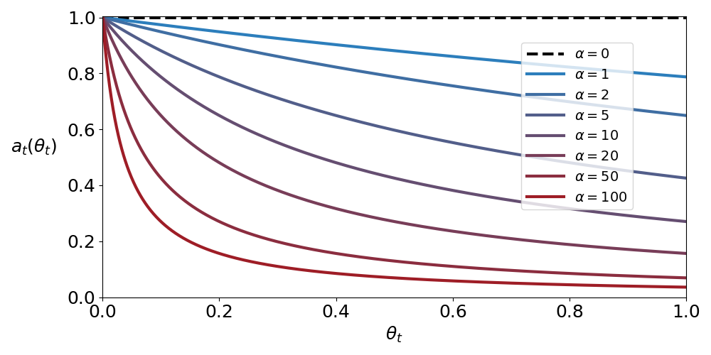
Fig. 2 shows the optimal social activity as a function of the weighted density of infected neighbors $\theta$, for different choices of the parameter $\alpha$. One can see that optimal social activity always decreases as the weighted density of infected neighbors increases, but its functional form depends on $\alpha$: optimal social activity decreases slowly or more abruptly when the average cost of the infection is small or large, respectively. In particular, when $\alpha$ is small, the optimal social activity decreases linearly with $\alpha$. We also tested the effect of the discount factor $\delta$ (not shown), which, in the range of values we consider for $\delta$ (see next Section) is negligible.

Finally, one can assume a homogeneous mixing hypothesis, meaning that all nodes are equal and one can approximate the degree of each node with the average degree of the network $\langle k\rangle$. Under this assumption, all individuals adopt the same social activity $a_{t}$ and the weighted density of infected neighbors becomes $\theta_{t}=a_{t}i_{t}$ where $i_{t}$ is the fraction of infected individuals in the population (prevalence) at time $t$. The homogeneous mean-field (MF) model is summarized by the following set of equations:

$$s_{t+1}=s_{t}-\beta\langle k\rangle a^{2}_{t}s_{t}i_{t}$$ (9a)

$$i_{t+1}=i_{t}+\beta\langle k\rangle a^{2}_{t}s_{t}i_{t}-\mu i_{t}$$ (9b)

$$r_{t+1}=r_{t}+\mu i_{t}$$ (9c)

$$a_{t+1}=\frac{1}{1+\alpha\delta\beta\langle k\rangle\theta_{t}}$$ (9d)

$$\theta_{t}=a_{t}i_{t}$$ (9e)

Again, Eq. (9d) is the equivalent of Eqs. (7) and (8d) in the homogeneous mixing hypothesis: at each time step $t$, individuals choose their optimal social activity depending only on the prevalence and other individuals’ social activity.

Therefore, we consider three different scenarios of awareness: i) In the homogeneous mixing case, individuals know the fraction of infected individuals in the population, ii) in the global (heterogeneous mean-field) case, individuals know how likely an individual is to be infected based on their degree, and iii) in the local awareness (quenched network) case, individuals know which of their contacts are infected on a per-individual basis.

2.4 Model calibration

We consider a time step to be equal to one day. We calibrate the MF model on a disease having basic reproduction number $R_{0}=3$ in absence of any mitigation measure, implying that a single infection case is expected, on average, to generate three new cases in a population of fully susceptible individuals. We set $\mu=1/10$, thus assuming an average infectious period equal to 10 days. The choices of $R_{0}$ and $\mu$ imply, for the MF model, a value of the infection rate $\beta=0.3/\langle k\rangle$, where $\langle k\rangle$ represents the average number of contacts per day. We fix $\langle k\rangle=17.4$ (see Methods for more information on network generation), thus obtaining $\beta=0.017$. The choice of the discount factor $\delta$ is more challenging and will be addressed later in this Section, after discussing the two main simplifying assumptions of our model in detail. Our choice for the epidemiological parameters is compatible with estimates of $R_{0}$ and $\mu$ for SARS-CoV-2 [36, 37, 38], and, more in general, with a typical rapidly transmitted respiratory infection, such as influenza [39].

A first simplifying assumption is to consider behavior to be homogeneous across all health states. While this assumption may not be realistic, other choices are also problematic. For instance, one could assume that infected individuals would always choose a maximum social activity $a=1$, since they can no longer get infected. Our assumption of considering that $S$ and $I$ individuals optimize in the same way their behavior is compatible with either individuals not knowing their health state (a concrete possibility in case of asymptomatic infections), or altruistic behavior. We also stress that assuming $a_{t}$ to be the same for all individuals does not necessarily mean that all individuals behave in the same way. Finally, we remark that the behavior of $R$ individuals is irrelevant since they do not participate in active links.

Second, individuals believe that current conditions (i.e. the sizes of the $S$, $I$ and $R$ compartments and the present value of $a_{t}$) will remain unchanged when planning. One might argue that this assumption is only realistic in the near future, however, in our model, the future utility gets exponentially discounted because of the term $\delta^{\Delta t}$ in Eq. (3). So although predictions are based on conditions that might not be valid in the distant future, they have less and less impact as they get further apart in time. On the other hand, assuming that individuals predict the future prevalence of the disease (for instance by means of the SIR model itself, [21]) can be equally unrealistic, since they may not know, for instance, the transmission and recovery rates.

Moreover, it seems unlikely that individuals take extended periods of time into account when planning. Some models address this issue by fixing a finite planning horizon, i.e. choosing the number of future days that are taken into account when planning [40]. However, this choice has two drawbacks: i) it adds another parameter to the model (the planning horizon), making it more difficult to fit with empirical data, and ii) it implies that future expected utility abruptly drops to zero when the planning horizon is reached. Instead, the discount factor $\delta$ ensures that future expected utility gradually decreases over time. Also, we emphasize that, since we consider an infinite planning horizon, in our model behavioral response is ultimately caused by discounting. In fact, if there was no discounting, limiting social activity would delay the infection, but the cost of infection would not change with time, so there would be no incentive to react to the spread of the disease.

This assumption has thus an impact on the plausible values of the discount factor $\delta$, which we choose to be rather small with respect to previous modeling approaches [19, 21, 32]. Note that in our model the discount factor includes both the standard economic discounting of the future and the expectations for a cure or a vaccine. In general, we set $\delta=0.9$, and test the robustness of the model in the range $\delta\in[0.8,0.95]$, observing no qualitative changes. With $\delta=0.9$, the utility one week from now weighs about 48% of today’s utility, this becomes 23% after two weeks and 4% after a month. This choice ensures that the planning horizon of individuals is actually finite so that they do not speculate about the distant future.

Figure 3: Equivalent social activity $a_{eq}$ corresponding to different values of $\alpha$ (dashed line). The dashed line represents the solution of Eq. (10). We set $\delta=0.9$. The color gradient is based on the values of $a_{eq}$ on the y-axis.

Finally, we address the issue of interpretability of the $\alpha$ parameter, which currently lacks a scale to be compared to (i.e. we have not yet determined which values of $\alpha$ should be associated with minor illnesses and which with more serious ones). To this aim, we define the equivalent social activity $a_{eq}$ as the value of the social activity for which the utility lost in one day due to the reduction of social activity $U_{a}(a_{eq})$ (given by Eq. (2)) is equal to $U_{I}$. To put it in other terms, $a_{eq}$ is the value of social activity for which there is no preferable choice in terms of utility between getting infected and spending a period corresponding to the average infectious period with social activity $a_{eq}$. This means that, with our choice of the utility function, $a_{eq}$ can be determined numerically as the root of the equation ${log(a_{t})-a_{t}+1+U_{I}=0}$. By using Eq. (5), we can express the previous equation in terms of $\alpha$, obtaining

$$log(a_{t})-a_{t}+1+\left[1-\delta(1-\mu)\right]\alpha=0.$$ (10)

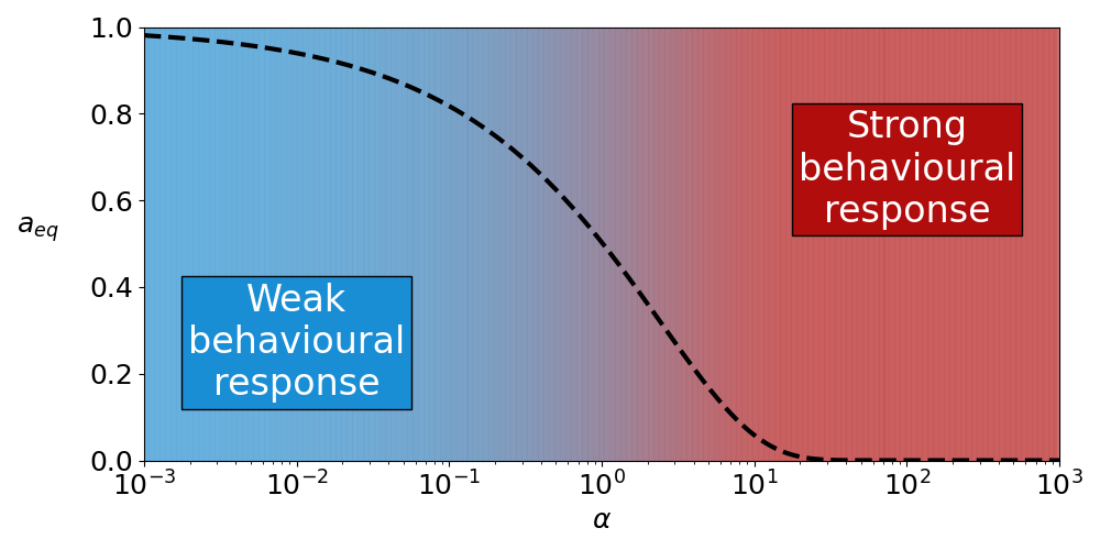
Fig. 3 shows the equivalent social activity corresponding to different values of $\alpha$ with $\delta=0.9$. Intuitively, $a_{eq}$ decreases as the average infection cost increases: individuals are not willing to reduce their social activity if the infection cost is small. However, it is interesting to note that the dependency on $\alpha$ is weak, due to the choice of the logarithmic form of the utility function. Individuals are not willing to significantly decrease their social activity for $\alpha\lessapprox 10^{-2}$, regardless of the infection probability (prevalence). They gradually decrease their social activity as a function of $\alpha$, until they are willing to reduce it to almost zero for $\alpha\gtrapprox 10$. For these values of $\alpha$, individuals consider becoming infected as serious as having virtually no social activity. We stress that this does not necessarily mean that individuals will choose to isolate (i.e., choose zero social activity) to avoid infection since the probability of getting infected is usually small ($P_{I}\ll 1$).

Here, we are interested in the regime for which there is a strong behavioral response (highlighted in red in Fig. 3), since behavior only becomes relevant when $a_{eq}\ll 1$. Also, we observe that only for high values of $\alpha$ (about $\alpha\simeq 100$ in the simulations presented in the next section) behavioral response based on local awareness is strong enough to prevent the epidemic from spreading. Therefore we will focus on the range ${0.1<\alpha<100}$.

2.5 Numerical simulations

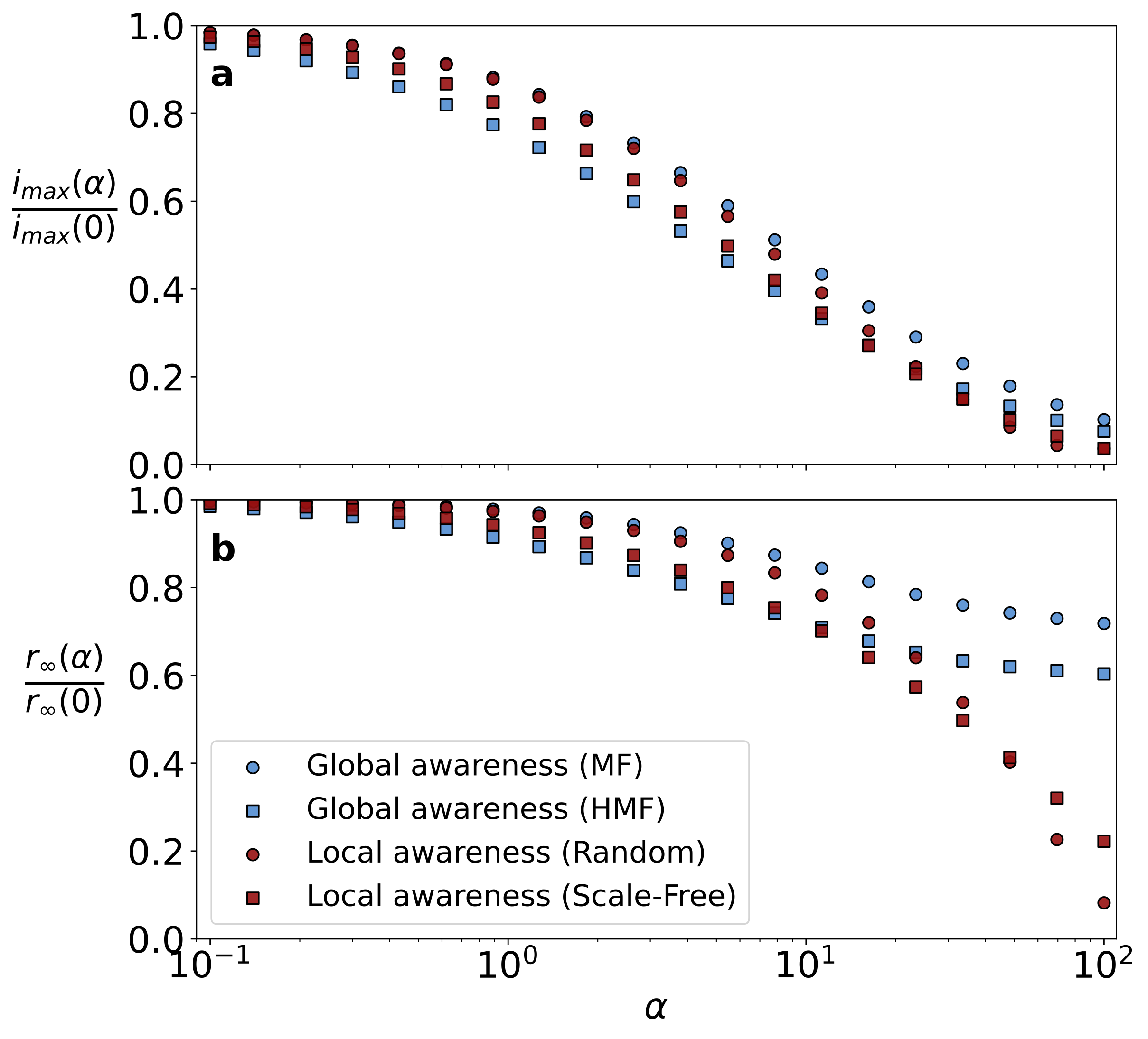
We will now show the results of numerical simulations of the model. We will consider the following four settings for the substrate of the epidemic: homogeneous mean-field (MF), heterogeneous mean-field (HMF) on a scale-free network, quenched random networks, and quenched scale-free networks, see Methods for details of the numerical simulations. The former two cases (annealed networks) represent global awareness, and the latter two cases (quenched networks) stand for local awareness.

Figure 4: Ratio between the peak prevalence $i_{max}$ (a) or the final attack rate $r_{\infty}$ (b) obtained for a given value of $\alpha$ and that corresponding to $\alpha=0$ (no behavioral response). We set $\delta=0.9$. Error bars are calculated as the standard error of the mean, not shown as smaller than points in the plot.

We quantify the outcome of the epidemic spread by two key quantities: the peak prevalence $i_{max}$, corresponding to the maximum number of infected individuals at the same time, and the final attack rate $r_{\infty}$, which corresponds to the limit $t\to\infty$ of the fraction of recovered individual $r_{t}$ and represents the total fraction of the population that has been infected by the disease. Notice that the peak prevalence can be related to the maximum capacity of the health system at the peak of the epidemic, while the final attack rate can be directly related to the number of deceased individuals. Since we will consider the ratio between different settings (corresponding to different values of $\alpha$), our results can be directly interpreted in this sense.

The main effect of behavioral change is to flatten the epidemic curve, lowering the peak prevalence and delaying the moment when the peak is reached. This effect is clearly shown in Fig. 4(a), in which we plot the peak prevalence $i_{max}$ as a function of $\alpha$. One can see that with a stronger behavioral response (larger $\alpha$) the peak prevalence decreases, thus indicating that behavioral responses flatten the epidemic curve. We also note no significant differences between global and local awareness.

In Fig. 4(b) we plot how the final attack rate $r_{\infty}$ changes with $\alpha$, showing that for both global and local awareness, $r_{\infty}$ decreases as the infection cost increases. However, the effects of behavioral change on $r_{\infty}$ are much stronger for the quenched case (local awareness) than the mean-field one (global awareness). The effect is particularly evident in the regime of strong behavioral response (large $\alpha$ for which $a_{eq}\ll 1$)), where the epidemic is almost suppressed when the awareness is local, while if individuals have only global awareness of the prevalence, the reduction in the final attack rate is relatively small.

The stronger effect for local awareness can be attributed to the more fine-grained behavioral response: individuals in direct contact with local outbreaks reduce their social activity, hampering early disease propagation. Therefore, even when the prevalence is low in the population and localized in a few individuals, the behavioral response of the neighbors of the infected individuals is sufficient to curb the disease spreading. In contrast, within the global setting, the prevalence has to grow enough in the population (in a specific degree class in the HMF case) in order to trigger a behavioral response from individuals. The possible presence of clusters (groups of highly-connected nodes) in the quenched networks acts similarly: when the behavioral response is strong (large $\alpha$ regime), the epidemic can not escape from the cluster where it started, but it dies out after exhausting the reservoir of susceptible individuals inside the cluster. The difference between local and global awareness instead disappears when the behavioral response is weak (small $\alpha$ values). In this regime, indeed, it is necessary that a considerable fraction of nodes is infected before triggering the behavioral response, so that many susceptible individuals will likely be in contact with several infected ones, a situation similar to the annealed network scenario.

3 Discussion

Our study aimed at bridging classical epidemic modelling, in which the transmission rate is modulated by some nonlinear function of the prevalence, and epi-economic models. These two approaches have been reported to largely operate in isolation and even to display, to some extent, a lack of consensus [41, 42]. We adopt the epi-economic framework, in which behavior is adopted by following a forward-looking approach, but we made some simplifying assumptions that allow us to describe the optimal behavior (i.e., the optimal degree of social activity) by analytical expressions. Crucially, we go beyond the homogeneous mixing hypothesis usually assumed in epi-economic models and test different degrees of heterogeneity in the population: local and global (degree-based) awareness.

We show that, if individuals expect current conditions to be stationary when planning, it is possible to find an analytical expression for the optimal social activity $a_{t}$ (Eq. (6)), that depends on the infection cost $\alpha$, the discount factor $\delta$, and infection probability $P_{I}(t)$. We note that the functional form of $a_{t}$ is not surprising. In fact, behavioral change models based on prevalence-dependent transmission rates have been using transmission rates of the form $A/(1+Bi_{t})$ for decades [43, 44]. However, in our model, the social activity does not depend solely on prevalence, but also on the current behavioral choices of the population, so changes in the prevalence are more relevant when collective behavior favors disease transmission ($a_{t}\simeq 1$) and become less and less relevant as behavior changes limiting the probability of infection ($a_{t}\ll 1$).

Moreover, we operationalize the infection probability in three different settings, local, global (HMF case), and homogeneous behavioral responses. We provide a simple interpretation for the infection cost $\alpha$ in terms of an equivalent social activity $a_{eq}$, defined as the acceptable social activity equivalent to the risk of infection. Such equivalence allows us to distinguish regimes of weak and strong behavioral responses. Finally, we quantify the effect of behavior change on the final attack rate of the disease in the regime of strong behavioral response, showing that local awareness allows for a much stronger outbreak reduction than global awareness.

Our model is not exempt from limitations. We discuss the validity of our two simplifying assumptions (homogeneous behavior across all health states and individuals believing current epidemic conditions will remain unchanged) in Section 2.4 (Model calibration). Furthermore, we assume that individuals are immediately aware of the health status of their peers (the global heterogeneous case or local prevalence). This is certainly unrealistic since some delay is to be expected between the moment an individual gets infected and the moment other individuals learn about it. However, we do not expect this to be particularly relevant for the mean-field versions of the model as that would just result in a different value of the weighted density of infected $\theta$. On the other hand, we believe that in a quenched setting the introduction of a delay between the moment a node gets infected and the moment its neighbors discover it would have a far stronger effect. In fact, since behavior is determined on a per-individual basis for simulations on a quenched network, nodes would not immediately limit their social activity when one of their neighbors gets infected, potentially resulting in nodes whose local prevalence is still low not reacting in time to the new infection even if global prevalence had already been high for a while. While the effects of delayed information in an epi-economic model that assumes homogeneous mixing have already been studied [45], future work could be devoted to investigating the effects of delayed information in a quenched setting.

Finally, we do not calibrate our model with empirical data. During the COVID-19 pandemic, a vast amount of empirical measurements of human behavior has become accessible, especially through mobile phone data [46]. These have been often used to incorporate human behavior into epidemic models in an effective manner, that is, by retrospectively integrating the observed changes in behavior, for instance, the reduction in movements, into disease dynamics [37, 47, 48]. However, epi-economic models would require rather different, and more granular, empirical measures of human behavior, aimed at quantifying individual future expectations and their heterogeneity in a population. Previous studies including game-theoretic behavioral changes have typically explored different scenarios, relying on assumed values for the parameters that regulate the behavioral responses [24, 21]. However, empirical measurements for these parameters, such as the expected cost of infection, remain scarce.

Our model depends only on two key parameters, the infection cost $\alpha$ and the discount factor $\delta$, which makes our model very parsimonious in terms of parameterization needs. To this aim, thanks to the equivalence between infection cost $\alpha$ and social activity we developed, the former could be estimated by means of surveys, by asking individuals how many days they would accept to isolate in order to avoid the infection [32]. The discount factor $\delta$ could be more difficult to estimate since it includes the expectations for a future cure. Previous studies have assumed standard values of $\delta$ but more work is needed to understand how $\delta$ may vary across epidemic scenarios, depending on the severity of the disease. In general, we remark that data quality is crucial to assess parameters of epidemiological models even in very simple settings, such as the basic reproduction number $R_{0}$ [49].

In conclusion, our study provides the description of a simple, yet a realistic model of forward-looking behavior that can be integrated into large-scale network epidemic models [50], contributing an additional layer of realism to models used to inform policymakers.

4 Methods

4.1 Derivation of closed-form objective function

In this section, we will present the derivation of the closed-form expression of the objective function $J$, defined in Eq. (3). The objective function is composed of two terms. The term involving $U_{a}$ depends neither on time (we assumed individuals to believe current conditions to persist in the future) nor on the health state (we assumed social activity to be homogeneous across all health states), so it is just a geometric series:

$$\mathbb{E}\sum_{\Delta t=0}^{\infty}\delta^{\Delta t}U_{a}(t)=\frac{U_{a}(t)}{1-\delta}$$ (11)

Let’s now focus on the term involving $U_{H}$. First, we will calculate the average cost of infection, which we indicate by $\alpha$. Considering an individual that has just transitioned from the $S$ state to the $I$ state, for each day spent in the infected state the individual gets a penalty of magnitude $U_{I}$, as for Eq. (1). Each day they recover from the disease with probability $\mu$, meaning that the probability of being still infected after $\Delta t$ days is $(1-\mu)^{\Delta t}$. Since after $\Delta t$ days the utility gets discounted by a factor $\delta^{\Delta t}$, the average total loss of utility caused by an infection is:

$$\alpha\equiv U_{I}\sum_{\Delta t=0}^{\infty}[\delta(1-\mu)]^{\Delta t}=\frac{U_{I}}{1-\delta(1-\mu)}.$$ (12)

The average cost of infection (here defined positive, to be subtracted in the expected utility) is thus proportional to the penalty $U_{I}$ and it becomes smaller for increasing discount factor $\delta$ and recovery rate $\mu$.

Let’s now consider an $S$ individual that is evaluating their expected utility loss because of the risk of infection at time $t$. If an $S$ individual gets infected $\Delta t$ days from $t$, the expected penalty (given by Eq. (12)) gets discounted by a factor $\delta^{\Delta t}$. The remaining term to close the calculation is the probability of becoming infected after $\Delta t$ time steps. Let $P_{I}(t)$ be the probability of becoming infected in one time step at time $t$ (the time in which the expected utility is evaluated), which is assumed to remain constant in the future (since individuals believe the current prevalence, as well as other individuals’ social activity, will persist). The probability of becoming infected after $\Delta t$ time steps is thus equal to $P_{I}(t)(1-P_{I}(t))^{\Delta t-1}$ (individuals must not have already been infected for the first $\Delta t-1$ time steps). Therefore, the expected utility loss due to the risk of infection is equal to the average loss for infection $\alpha$, multiplied by the probability it happens after $\Delta t$ time steps, and thus discounted by $\delta^{\Delta t}$:

$$\mathbb{E}\sum_{\Delta t=0}^{\infty}\delta^{\Delta t}U_{H}(t)=-\delta P_{I}(t)\sum_{\Delta t=1}^{\infty}[\delta(1-P_{I}(t))]^{\Delta t-1}\alpha.$$ (13)

By solving the geometric series and assuming that the probability of an $S$ individual getting infected at time $t$ is small, $P_{I}(t)\ll 1$, one obtains

$$\mathbb{E}\sum_{\Delta t=0}^{\infty}\delta^{\Delta t}U_{H}(t)=-\frac{\alpha\delta}{1-\delta}P_{I}(t).$$ (14)

Combining Eq. (11) and Eq. (14) into Eq. (3), the closed-form expression for $J$ is obtained:

$$J(t)=\frac{1}{1-\delta}\left[U_{a}(t)-\alpha\delta P_{I}(t)\right].$$ (15)

4.2 Details of numerical simulations

Here we provide details about how we carried numerical simulations out. Simulations on quenched networks (both the random and the scale-free case) are performed by looping over infected nodes and their neighbors and choosing whether transitions happen or not based on the generation of a random variable. At each time step contagion occurs in each connected pair of one $S$ node and $I$ node with probability $\beta$ and each $I$ individual has a probability $\mu$ of recovery. Mean-field simulations are based on equations 8a - 8e (HMF) and 9a - 9d (MF).

All simulations whose results are presented in Fig. 4 are performed with $\beta\langle k\rangle=0.3$, $\mu=0.1$, and initial conditions ${i_{0}=0.01}$ and $a_{i,0}=1$ for all nodes. For simulations on quenched networks, results correspond to ensemble averages over $10^{3}$ simulations (and thus $10^{3}$ quenched networks). All networks have $N=10^{5}$ nodes. Scale-free networks are generated using the configuration model [51] implemented in the NetworkX Python package [52] with minimum degree $k_{min}=5$, maximum degree ${k_{max}\simeq\sqrt{N}=316}$ and exponent $\gamma=2.1$. The resulting expected average degree is $\langle k\rangle=17.4$. The same value of $\langle k\rangle$ is used for random networks too.

5 Funding

This work did not receive any funding.

6 Author contributions statement

L.A.N.F. developed the epidemic model, performed analytical and numerical experiments, interpreted the results, and wrote the initial draft of the manuscript. M.S. and M.T. conceived and designed the study, supervised the research, interpreted the results, and wrote the manuscript. All authors read and approved the final version of the manuscript.

7 Code availability

The code to reproduce the results of the manuscript is available at https://github.com/lorenzoamir/EpiNetworkPaper

References

- [1] Neil M. Ferguson. Capturing human behaviour. Nature, 446:733–733, 2007.
- [2] Chansung Kim, Seung Hoon Cheon, Keechoo Choi, Chang-Hyeon Joh, and Hyuk-Jin Lee. Exposure to fear: Changes in travel behavior during mers outbreak in seoul. KSCE Journal of Civil Engineering, 21(7):2888–2895, 2017.
- [3] Alfred W. Crosby. America’s Forgotten Pandemic: The Influenza of 1918. Cambridge University Press, 2 edition, 2003.
- [4] G. James Rubin, Richard Amlôt, Lisa A. Page, and Simon Wessely. Public perceptions, anxiety, and behaviour change in relation to the swine flu outbreak: cross sectional telephone survey. The BMJ, 339, 2009.
- [5] James Jones and Marcel Salathé. Early assessment of anxiety and behavioral response to novel swine-origin influenza a(h1n1). PloS one, 4:e8032, 12 2009.
- [6] Ymir Vigfusson, Thorgeir A Karlsson, Derek Onken, Congzheng Song, Atli F Einarsson, Nishant Kishore, Rebecca M Mitchell, Ellen Brooks-Pollock, Gudrun Sigmundsdottir, and Leon Danon. Cell-phone traces reveal infection-associated behavioral change. Proceedings of the National Academy of Sciences, 118(6):e2005241118, 2021.
- [7] Nicola Perra. Non-pharmaceutical interventions during the covid-19 pandemic: A review. Physics Reports, 913:1–52, 2021.
- [8] Sebastian Funk, Shweta Bansal, Chris T Bauch, Ken TD Eames, W John Edmunds, Alison P Galvani, and Petra Klepac. Nine challenges in incorporating the dynamics of behaviour in infectious diseases models. Epidemics, 10:21–25, 2015.
- [9] Sebastian Funk, Marcel Salathé, and Vincent Jansen. Modelling the influence of human behaviour on the spread of infectious diseases: A review. Journal of the Royal Society Interface, 7:1247–56, 09 2010.
- [10] Frederik Verelst, Lander Willem, and Philippe Beutels. Behavioural change models for infectious disease transmission: A systematic review (2010-2015). Journal of The Royal Society Interface, 13, 12 2016.
- [11] Piero Manfredi and Alberto D’Onofrio. Modeling the interplay between human behavior and the spread of infectious diseases. Springer Science & Business Media, 2013.
- [12] Nicola Perra, Duygu Balcan, Bruno Gonçalves, and Alessandro Vespignani. Towards a characterization of behavior-disease models. PloS one, 6(8):e23084, 2011.
- [13] Valeria d’Andrea, Riccardo Gallotti, Nicola Castaldo, and Manlio De Domenico. Individual risk perception and empirical social structures shape the dynamics of infectious disease outbreaks. PLoS Computational Biology, 18(2):e1009760, 2022.
- [14] Clara Granell, Sergio Gómez, and Alex Arenas. Dynamical interplay between awareness and epidemic spreading in multiplex networks. Phys. Rev. Lett., 111:128701, Sep 2013.
- [15] Joshua M Epstein, Jon Parker, Derek Cummings, and Ross A Hammond. Coupled contagion dynamics of fear and disease: mathematical and computational explorations. PloS one, 3(12):e3955, 2008.
- [16] Sebastian Funk, Erez Gilad, Chris Watkins, and Vincent AA Jansen. The spread of awareness and its impact on epidemic outbreaks. Proceedings of the National Academy of Sciences, 106(16):6872–6877, 2009.
- [17] Piero Poletti, Marco Ajelli, and Stefano Merler. Risk perception and effectiveness of uncoordinated behavioral responses in an emerging epidemic. Mathematical Biosciences, 238(2):80–89, 2012.
- [18] Piero Poletti, Marco Ajelli, and Stefano Merler. The effect of risk perception on the 2009 h1n1 pandemic influenza dynamics. PloS one, 6(2):e16460, 2011.
- [19] Eli P. Fenichel, Carlos Castillo-Chavez, M. G. Ceddia, Gerardo Chowell, Paula A. Gonzalez Parra, Graham J. Hickling, Garth Holloway, Richard Horan, Benjamin Morin, Charles Perrings, Michael Springborn, Leticia Velazquez, and Cristina Villalobos. Adaptive human behavior in epidemiological models. Proceedings of the National Academy of Sciences, 2011.
- [20] David Aadland, David C. Finnoff, and Kevin X.D. Huang. Syphilis cycles. The B.E. Journal of Economic Analysis & Policy, 13(1):297–348, 2013.
- [21] Maryam Farboodi, Gregor Jarosch, and Robert Shimer. Internal and external effects of social distancing in a pandemic. Journal of Economic Theory, 196:105293, 2021.
- [22] Alberto Bisin and Andrea Moro. Spatial-SIR with Network Structure and Behavior: Lockdown Policies and the Lucas Critique. Journal of Economic Behavior & Organization, 198:370–388, June 2022.
- [23] Kathinka Frieswijk, Lorenzo Zino, Mengbin Ye, Alessandro Rizzo, and Ming Cao. A mean-field analysis of a network behavioral–epidemic model. IEEE Control Systems Letters, 6:2533–2538, 2022.
- [24] Mengbin Ye, Lorenzo Zino, Alessandro Rizzo, and Ming Cao. Game-theoretic modeling of collective decision making during epidemics. Physical Review E, 104(2):024314, 2021.
- [25] Peter Bearman, James Moody, and Katherine Stovel. Chains of affection: The structure of adolescent romantic and sexual networks. American Journal of Sociology, 110, 07 2004.
- [26] James Jones and Mark Handcock. An assessment of preferential attachment as a mechanism for human sexual network formation. Proceedings. Biological sciences / The Royal Society, 270:1123–8, 06 2003.
- [27] Fredrik Liljeros, Christofer Edling, Luís Amaral, H. Stanley, and Yvonne Aberg. The Web of Human Sexual Contacts. Nature, 411, 06 2001.
- [28] Lauren Ancel Meyers, Babak Pourbohloul, Mark EJ Newman, Danuta M Skowronski, and Robert C Brunham. Network theory and sars: predicting outbreak diversity. Journal of theoretical biology, 232(1):71–81, 2005.
- [29] William Ogilvy Kermack, A. G. McKendrick, and Gilbert Thomas Walker. A contribution to the mathematical theory of epidemics. Proceedings of the Royal Society of London. Series A, Containing Papers of a Mathematical and Physical Character, 115(772):700–721, 1927.
- [30] Raghavendra Tirupathi, Kavya Bharathidasan, Venkataraman Palabindala, Sohail Abdul Salim, and Jaffar A Al-Tawfiq. Comprehensive review of mask utility and challenges during the covid-19 pandemic. Infez Med, 28(suppl 1):57–63, 2020.
- [31] Eli P. Fenichel. Economic considerations for social distancing and behavioral based policies during an epidemic. Journal of Health Economics, 32(2):440–451, 2013.
- [32] Martin F. Quaas, Jasper N. Meya, Hanna Schenk, Björn Bos, Moritz A. Drupp, and Till Requate. The social cost of contacts: Theory and evidence for the first wave of the covid-19 pandemic in germany. PLOS ONE, 16(3):1–29, 03 2021.
- [33] Sergio Gómez, Alexandre Arenas, Javier Borge-Holthoefer, Sandro Meloni, and Yamir Moreno. Discrete-time markov chain approach to contact-based disease spreading in complex networks. EPL (Europhysics Letters), 89(3):38009, 2010.
- [34] Marián Boguná, Claudio Castellano, and Romualdo Pastor-Satorras. Langevin approach for the dynamics of the contact process on annealed scale-free networks. Physical Review E, 79(3):036110, 2009.
- [35] Albert-László Barabási. Network Science. Cambridge University Press, 2016.
- [36] Stephen A Lauer, Kyra H Grantz, Qifang Bi, Forrest K Jones, Qulu Zheng, Hannah R Meredith, Andrew S Azman, Nicholas G Reich, and Justin Lessler. The incubation period of coronavirus disease 2019 (covid-19) from publicly reported confirmed cases: estimation and application. Annals of internal medicine, 172(9):577–582, 2020.
- [37] Nicolò Gozzi, Michele Tizzoni, Matteo Chinazzi, Leo Ferres, Alessandro Vespignani, and Nicola Perra. Estimating the effect of social inequalities on the mitigation of covid-19 across communities in santiago de chile. Nature communications, 12(1):1–9, 2021.
- [38] Andrew William Byrne, David McEvoy, Aine B Collins, Kevin Hunt, Miriam Casey, Ann Barber, Francis Butler, John Griffin, Elizabeth A Lane, Conor McAloon, et al. Inferred duration of infectious period of sars-cov-2: rapid scoping review and analysis of available evidence for asymptomatic and symptomatic covid-19 cases. BMJ open, 10(8):e039856, 2020.
- [39] Justin Lessler, Nicholas G Reich, Derek AT Cummings, New York City Department of Health, and Mental Hygiene Swine Influenza Investigation Team. Outbreak of 2009 pandemic influenza a (h1n1) at a new york city school. New England Journal of Medicine, 361(27):2628–2636, 2009.
- [40] Luis G Nardin, Craig R Miller, Benjamin J Ridenhour, Stephen M Krone, Paul Joyce, and Bert O Baumgaertner. Planning horizon affects prophylactic decision-making and epidemic dynamics. PeerJ, 4:e2678, 2016.
- [41] Michael E. Darden, David Dowdy, Lauren Gardner, Barton H. Hamilton, Karen Kopecky, Melissa Marx, Nicholas W. Papageorge, Daniel Polsky, Kimberly A. Powers, Elizabeth A. Stuart, and Matthew V. Zahn. Modeling to inform economy-wide pandemic policy: Bringing epidemiologists and economists together. Health Economics, 31(7):1291–1295, 2022.
- [42] Eleanor J. Murray. Epidemiology’s Time of Need: COVID-19 Calls for Epidemic-Related Economics. Journal of Economic Perspectives, 34(4):105–20, November 2020.
- [43] Vincenzo Capasso and Gabriella Serio. A generalization of the kermack-mckendrick deterministic epidemic model. Mathematical Biosciences, 42(1):43–61, 1978.
- [44] W. Wang. Modeling adaptive behavior in influenza transmission. Mathematical Modelling of Natural Phenomena, 7(3):253–262, 2012.
- [45] Ronan F. Arthur, James H. Jones, Matthew H. Bonds, Yoav Ram, and Marcus W. Feldman. Adaptive social contact rates induce complex dynamics during epidemics. PLOS Computational Biology, 17(2):1–17, 02 2021.
- [46] Nuria Oliver, Bruno Lepri, Harald Sterly, Renaud Lambiotte, Sébastien Deletaille, Marco De Nadai, Emmanuel Letouzé, Albert Ali Salah, Richard Benjamins, Ciro Cattuto, et al. Mobile phone data for informing public health actions across the covid-19 pandemic life cycle, 2020.
- [47] Pierre Nouvellet, Sangeeta Bhatia, Anne Cori, Kylie EC Ainslie, Marc Baguelin, Samir Bhatt, Adhiratha Boonyasiri, Nicholas F Brazeau, Lorenzo Cattarino, Laura V Cooper, et al. Reduction in mobility and covid-19 transmission. Nature communications, 12(1):1–9, 2021.
- [48] Laura Di Domenico, Giulia Pullano, Chiara E Sabbatini, Pierre-Yves Boëlle, and Vittoria Colizza. Impact of lockdown on covid-19 epidemic in île-de-france and possible exit strategies. BMC medicine, 18(1):1–13, 2020.
- [49] Michele Starnini, Alberto Aleta, Michele Tizzoni, and Yamir Moreno. Impact of data accuracy on the evaluation of covid-19 mitigation policies. Data & Policy, 3:e28, 2021.
- [50] Serina Chang, Emma Pierson, Pang Wei Koh, Jaline Gerardin, Beth Redbird, David Grusky, and Jure Leskovec. Mobility network models of covid-19 explain inequities and inform reopening. Nature, 589(7840):82–87, 2021.
- [51] M. E. J. Newman. The structure and function of complex networks. SIAM Review, 45(2):167–256, 2003.
- [52] Aric A. Hagberg, Daniel A. Schult, and Pieter J. Swart. Exploring network structure, dynamics, and function using networkx. In Gaël Varoquaux, Travis Vaught, and Jarrod Millman, editors, Proceedings of the 7th Python in Science Conference, pages 11 – 15, Pasadena, CA USA, 2008.