Rationality and Parametrizations of Algebraic Curves under Specializations

Abstract.

Rational algebraic curves have been intensively studied in the last decades, both from the theoretical and applied point of view. In applications (e.g. level curves, linear homotopy deformation, geometric constructions in computer aided design, etc.), there often appear unknown parameters. It is possible to adjoin these parameters to the coefficient field as transcendental elements. In some particular cases, however, the curve has a different behavior than in the generic situation treated in this way. In this paper, we show when the singularities and thus the (geometric) genus of the curves might change. More precisely, we give a partition of the affine space, where the parameters take values, so that in each subset of the partition the specialized curve is either reducible or its genus is invariant. In particular, we give a Zariski-closed set in the space of parameter values where the genus of the curve under specialization might decrease or the specialized curve gets reducible. For the genus zero case, and for a given rational parametrization, a better description is possible such that the set of parameters where Hilbert’s irreducibility theorem does not hold can be isolated, and such that the specialization of the parametrization parametrizes the specialized curve. We conclude the paper by illustrating these results by some concrete applications.

1. Introduction

The study and analysis of the behavior of algebraic or algebraic-geometric objects under specializations is of great interest from a theoretical, computational or applied point of view. For instance, some techniques for computing resultants, gcds, or polynomial factorizations, rely on Hensel’s lemma or the Chinese remainder theorem (see e.g. [11], [39]). From a more theoretical point of view, also computational, it is important to control, for instance, when a resultant, or more generally a Gröbner basis with parameters, specializes properly (see e.g. [6], [17]). The question whether a given irreducible polynomial over $\mathbb{K}(a_{1},\ldots,a_{n})$ remains irreducible when the parameters are replaced by values in a field $\mathbb{K}$ was studied intensively by Hilbert [8] and Serre [31] and is the defining property of “Hilbertian fields”. The work of Serre can be seen in a more general context. With respect to applications, there is a vast amount of applications of algebraic curves involving parameters: level curves of surfaces [2], linear homotopy deformation of curves (see Section 7), curve recognition [34], geometric constructions in computer aided design, like offsets, conchoids, cissoids etc, where the final object depends on the distance, the focus, etc.; see e.g. [3], [4], [16], [19], [24]. Another type of applications is the computation with meromorphic functions in linear algebra (see [25]) or the rational solutions of functional algebraic equations (see Section 7).

In this work we study algebraic curves $\mathcal{C}(F)$ given as the zero-set of a polynomial

(1.1) $$F(x,y)=0~{}\text{ with }~{}F\in\mathbb{K}(a_{1},\ldots,a_{n})[x,y]$$

where $\mathbb{K}$ is a computable field of characteristic zero, $a_{1},\ldots,a_{n}$ are a set of parameters, and $F$ is irreducible over the algebraic closure of the coefficient field $\mathbb{K}(a_{1},\ldots,a_{n})$, denoted by $\overline{\mathbb{K}(a_{1},\ldots,a_{n})}$. In this paper, we focus on the problem that for certain values of the parameters $a_{1},\ldots,a_{n}$ the algebraic properties of the resulting curve do not coincide with the generic properties of $\mathcal{C}(F)$. More precisely, we define several Zariski-closed sets in the space of parameter values where non-generic behavior may appear. Of particular interest are the singularities, their multiplicities and their character. This leads to a partition of the affine space, where the parameters take values, so that in each subset of the partition the specialized curve is either reducible or its (geometric) genus is invariant. When the generic curve has genus zero, for a given rational parametrization can be given a better description. In particular, the set of parameters where Hilbert’s irreducibility theorem does not hold can be isolated. Moreover, the proper specialization of the rational parametrization is guaranteed.

In [30, 37] and references therein are studied algebraic curves and their rationality. The problem of finding rational parametrizations of plane curves is a classical problem and has already been studied by Hilbert [9], and more recently in [13], [21], [27],[28]. In addition, for evaluating the parameters, it is important to control field extensions which might be necessary for computing parametrizations. Optimal fields of parametrizations have been studied in [13] and [28]. When introducing parameters in the coefficients, new phenomena have to be considered and lead to Tsen’s study of finding solutions in a minimal field [7].

The structure of the paper is as follows. In Section 2 we present notations, preliminaries on algebraic curves and rational parametrizations. Of particular interest is the computation of the genus and a rational parametrization, if it exists. Some of the details are attached in the appendix A. In Section 3, we introduce the unspecified parameters and their specialization. The computation of the genus and rational parametrizations is followed to define several computable Zariski-open subsets $\Omega$ where the specialized curve behaves, up to irreducibility, as in the generic case. The actual computation of the genus is presented in Section 4. In Theorem 4.2 is shown that the genus of the specialized curve, where the parameters take values in $\Omega_{\mathrm{singOrd}}$, is less or equal to the generic genus or the defining polynomial is reducible. A direct corollary of that is that specialized curves of rational curves are also rational or reducible (Corollary 4.3). For values in a smaller set $\Omega_{\mathrm{genusOrd}}$, it is shown that the genus of the curve remains exactly the same, again up to irreducibibility, see Theorem 4.8. Section 5 is devoted to the case where the generic curve is rational; in this frame the irreducibility can be guaranteed. For some of the parameter values the genus may remain the same but an evaluation of the parametrization is not possible. In Theorem 5.5, however, is presented an open set where the specialization is possible and results in a parametrization of the specialized curve. These open sets can be recursively used for decomposing the whole parameter space as it is explained in Section 6. Applications as described above are presented by using illustrative examples in Section 7.

This manuscript is a self-contained work on the computation of the genus and rational parametrizations of algebraic curves involving parameters. Results from various mathematical disciplines are combined for this purpose and presented in a coherent way. A rigorous construction of such computable Zariski-open sets were, up to our knowledge, missing in the literature. The theorems mentioned in the previous paragraph are novel and can be directly applied in several interesting problems involving parametric curves.

2. Preliminaries and notation

Throughout this paper, the following notation will be used. $\mathbb{K}$ is a computable field of characteristic zero. We denote by $\mathbf{a}$ a tuple of parameters, and we represent by $\mathbb{L}$ the field extension $\mathbb{L}:=\mathbb{K}(\mathbf{a})$. In addition, we consider an algebraic element $\gamma$ over $\mathbb{L}$. Let $\mathbb{F}$ be the field $\mathbb{F}:=\mathbb{L}(\gamma)$. Furthermore, $K$ represents any field extension of $\mathbb{K}$. We denote by $\overline{K}$ the algebraic closure of $K$, similarly for any field appearing in the paper. $\mathbb{S}$ is the affine space

(2.1) $$\mathbb{S}=\overline{\mathbb{K}}^{\,\#(\mathbf{a})}$$

where $\mathbf{a}$ will take values.

For $G\in K[x,y]\setminus K$, we denote by $\mathcal{C}(G)$ the plane affine algebraic curve

$$\mathcal{C}(G)=\{p\in\overline{K}^{2}\,|\,G(p)=0\}.$$

We denote by $G^{h}(x,y,z)$ the homogenization of $G$, and by $G_{x},G_{y}$ (similarly for $G^{h}_{x},G^{h}_{y},G^{h}_{z}$) the partial derivative of $G$ w.r.t. $x$ and $y$ respectively. For a homogeneous polynomial $M\in K[x,y,z]\setminus\{0\}$, $\mathcal{C}(M)$ denotes the projective plane curve

$$\mathcal{C}(M)=\{p\in\mathbb{P}^{2}(K)\,|\,M(p)=0\}.$$

For polynomials $f,g$ in the variable $t$, and coefficients in an integral domain, we denote by $\mathrm{res}_{t}(f,g)$ the resultant of $f$ and $g$ w.r.t. $t$.

Let $\{f_{1},\ldots,f_{k}\}\subset K[\overline{v}]$, where $\overline{v}$ is a tuple of variables. We denote by $\mathbb{V}(f_{1},\ldots,f_{k})$ the zero set, over $\overline{K}$, of the polynomials $\{f_{1},\ldots,f_{k}\}$; similarly for $\mathbb{V}(\mathrm{I})$ where $\mathrm{I}$ is an ideal in $K[\overline{v}]$.

2.1. Rational Curves

Throughout this section, let $G\in K[x,y]\setminus K$ be irreducible over $\overline{K}$. A rational (affine) parametrization of the irreducible affine plane curve $\mathcal{C}(G)$ is a pair of rational functions $\mathcal{P}(t)\in\overline{K}(t)^{2}\setminus\overline{K}^{2}$ such that $G(\mathcal{P}(t))=0$. A rational (projective) parametrization of $\mathcal{C}(G^{h})$ is of form $\mathcal{Q}(h,t)=(p_{1}(h,t):p_{2}(h,t):p_{3}(h,t))$ where $p_{i}$ are homogeneous co-prime polynomials of the same degree over $\overline{K}$, not all zero, such that $G^{h}(\mathcal{Q})=0$. We observe that the degree, the irreducibility and the rationality of $\mathcal{C}(G)$ and $\mathcal{C}(G^{h})$ are equivalent. Moreover the parametrizations of $\mathcal{C}(G)$ and $\mathcal{C}(G^{h})$ relate each other by means of homogenizing and dehomogenizing. So, in the following we will focus on affine parametrizations.

The parametrization $\mathcal{P}(t)$ is called birational or proper if the map $\overline{K}\dashrightarrow\mathcal{C}(G);t\mapsto\mathcal{P}(t)$ is injective in a non–empty open Zariski subset of $\overline{K}$ (see e.g. [30] for further details). Curves admitting a rational parametrization are called rational, and they correspond to those of genus zero; note that the genus of $\mathcal{C}(G)$ is defined as the genus of $\mathcal{C}(G^{h})$. There exist algorithmic methods to compute the genus of an algebraic curves and to determine, when the genus is zero, a rational parametrization of the curve (see e.g. [13], [27], [28], [30]). In Appendix A we summarize the adjoint curves based method for parametrizing curves. Some of the ideas in this paper will use those methods.

In general, if one computes a parametrization $\mathcal{P}(t)$ of $\mathcal{C}(G)$, the ground field $K$ has to be extended (see e.g. Sections 4.7. and 4.8. in [30]). A subfield $\mathbb{E}$ of $\overline{K}$ is called a parametrizing field or field of parametrization of $\mathcal{C}(G)$ if there exists a parametrization of $\mathcal{C}(G)$ with coefficients in $\mathbb{E}$.

2.2. Fields of Parametrization

In this section, we work with the field $\mathbb{L}:=\mathbb{K}(\mathbf{a})$. Let $G\in\mathbb{L}[x,y]$ be an irreducible (over $\overline{\mathbb{L}}$) non-constant polynomial, and let us assume $\mathcal{C}(G)$ is a rational curve. We analyze the fields of parametrization of $\mathcal{C}(G)$.

$\overline{\mathbb{L}}$ is always a field of parametrization of $\mathcal{C}(G)$. Nevertheless, in [28] (see also Chapter 5 in [30]), the optimality of the fields of parametrization is analyzed and, as a consequence of Hilbert-Hurwitz Theorem (see [9]), there always exists a field extension of $\mathbb{L}$, of degree at most $2$, being a field of parametrization of $\mathcal{C}(G)$. Indeed, this field extension, of degree at most two, is the field extension used in Step (4), of the parametrization computation (see Subsection A.2), to express the simple point utilized in the parametrization of either the conic or the line.

We observe that if the two degree field extension is $\mathbb{L}(\alpha)$, with minimal polynomial $t^{2}+bt+c\in\mathbb{L}[t]$, then $\mathbb{L}(\alpha)=\mathbb{L}(\beta)$ where $\beta=\alpha+b/2$ which minimal polynomial is $t^{2}+c-b^{2}/4$. Therefore, the following holds.

Theorem 2.1.

1. If $\deg(\mathcal{C}(G))$ is odd then $\mathbb{L}$ is a field of parametrization.

2. If $\deg(\mathcal{C}(G))$ is even then either $\mathbb{L}$ is a field of parametrization or there exists $\delta\in\overline{\mathbb{L}}$ algebraic over $\mathbb{L}$, with minimal polynomial $t^{2}-\alpha\in\mathbb{L}[t]$, such that $\mathbb{L}(\delta)$ is a field of parametrization of $\mathcal{C}(G)$.

Remark 2.2.

Observe that the previous result is valid taking $\mathbb{L}$ as any field extension of $\mathbb{K}$.

The case where $\mathbf{a}$ contains a single element admits a particular treatment because of Tsen’s Theorem; we refer to [7] for this topic.

Corollary 2.3.

If $\#(\mathbf{a})=1$, then $\mathbb{L}$ is a field of parametrization of $\mathcal{C}(G)$.

Proof.

By Hilbert-Hurwitz Theorem (see e.g. Theorem 5.8. in [30] or Subsection A.2), $\mathcal{C}(G)$ is $\mathbb{L}$–birationally equivalent to either a line or a conic. So, fields of parametrization are preserved. In the line case, the result is clear. In the conic case, the result follows from Tsen’s Theorem (see e.g. Corollary 1.11. in [32]). ∎

Remark 2.4.

The proof of Tsen’s Theorem provides a method for computing an $\mathbb{L}$-simple point on the conic. An alternative approach for computing this point can be found in [12] and [33].

Remark 2.5.

In the following section we will work with $G\in\mathbb{K}[\mathbf{a},\gamma][x,y]$ where $\gamma$ is algebraic over $\mathbb{K}(\mathbf{a})$. In the case where $\#(\mathbf{a})=1$, we can view $\gamma$ as the only parameter and write $\mathbf{a}$ in terms of $\gamma$. More precisely, let $M(\mathbf{a},c)\in\mathbb{K}(\mathbf{a})[c]$ be the minimal polynomial of $\gamma$. We can view $M$ as rational expression in $\mathbf{a}$ and consider $H(a):=\operatorname{num}(M)(\mathbf{a}=a,c=\gamma)\in\mathbb{K}(\gamma)[a]$ as polynomial in $a$ with the root $\mathbf{a}$. Thus, $\mathbb{K}(\gamma,\mathbf{a}):\mathbb{K}(\gamma)$ is a field extension of degree $d\leq\deg_{c}(M)$. If $d=1$, by Corollary 2.3, $\mathbb{K}(\gamma)$ is a field of parametrization of $\mathcal{C}(G)$.

Remark 2.6.

In Corollary 2.3, we have seen that if $\#(\mathbf{a})=1$ then $\mathbb{L}$ is a field of parametrization. The following example shows that if $\#(a)>1$, in general, $\mathbb{L}$ is not a field of parametrization. We consider the conic defined by $F:=a_{1}x^{2}+a_{2}y^{2}-1$, and we see that it does not have a parametrization over $\mathbb{C}(a_{1},a_{2})$. Let us assume that $\mathbb{C}(a_{1},a_{2})$ is a field of parametrization of $\mathcal{C}(F)$, then $\mathcal{C}(F)$ has infinitely many point in $\mathbb{C}(a_{1},a_{2})^{2}$. $\mathcal{C}(F)$ can be properly parametrized by

$$\mathcal{P}:=\left(\sqrt{a_{1}}\,\frac{1-t^{2}}{t^{2}+1},\sqrt{a_{2}}\,\frac{2t}{t^{2}+1}\right),$$

which inverse is

$$\mathcal{P}^{-1}(x,y)=\frac{\sqrt{a_{2}}\,\left(\sqrt{a_{1}}+x\right)}{\sqrt{a_{1}}\,y}.$$

So, there are infinitely many points in $\mathcal{C}(F)\cap\mathbb{C}(a_{1},a_{2})^{2}$ that are injectively reachable, via $\mathcal{P}$, for $t\in\mathbb{C}(\sqrt{a_{1}},\sqrt{a_{2}})$. Indeed, note that all points of $\mathcal{C}(F)$, with the exception of $(-\sqrt{a_{1}},0)$, are reachable by $\mathcal{P}$. Let $t_{0}\in\mathbb{C}(\sqrt{a_{1}},\sqrt{a_{2}})\setminus\{0,\pm\mathrm{i}\}$ be one of these parameter values; say $\mathcal{P}(t_{0})=(x_{0},y_{0})\in\mathbb{C}(a_{1},a_{2})^{2}$. Then $t_{0}^{2}=(\sqrt{a_{1}}+x_{0})/(\sqrt{a_{1}}-x_{0})\in\mathbb{C}(\sqrt{a_{1}},a_{2}).$ For $x_{0}\neq 0$, it holds that $\sqrt{a_{1}}+x_{0}$, $\sqrt{a_{1}}-x_{0}$ are coprime (seen as polynomials in $\sqrt{a_{1}}$) and $t_{0}=\pm\sqrt{\tfrac{\sqrt{a_{1}}+x_{0}}{\sqrt{a_{1}}-x_{0}}}\notin\mathbb{C}(\sqrt{a_{1}},\sqrt{a_{2}})$, a contradiction. For $x_{0}=0$ we have the curve-points $(x_{0},y_{0})=(0,\pm 1/\sqrt{a_{2}})$ which are not in $\mathbb{C}(a_{1},a_{2})$.

3. Specializations

Throughout the paper, we will specialize the tuple of parameters $\mathbf{a}$ taking values in $\mathbb{S}$ (see (2.1)). We will write $\mathbf{a}^{0}$ to emphasize that the parameters in $\mathbf{a}$ have been substituted by elements in $\overline{\mathbb{K}}$. In the following we discuss different aspects on the specializations.

3.1. General statements

The elements in $\overline{\mathbb{K}}(\mathbf{a})$ are assumed to be represented in reduced form; that is, the numerator and denominator are assumed to be coprime. Then, for $f:=p/q\in\overline{\mathbb{K}}(\mathbf{a})$, where by assumption $\gcd(p,q)=1$, and for $\mathbf{a}^{0}\in\mathbb{S}$ (see (2.1)) such that $q(\mathbf{a}^{0})\neq 0$, we denote by $f(\mathbf{a}^{0})$ the $\overline{\mathbb{K}}$–element $p(\mathbf{a}^{0})/q(\mathbf{a}^{0})$.

We may need to work in the finite field extension $\mathbb{F}=\mathbb{L}(\gamma)$. Let $p(\mathbf{a},t)\in\mathbb{K}(\mathbf{a})[t]$, of degree $k$ in $t$, be the minimal polynomial of $\gamma$. We might simply write $p(t)$ instead of $p(\mathbf{a},t)$ and express it as

(3.1) $$p(t)=t^{k}+\frac{N_{k-1}(\mathbf{a})}{D_{k-1}(\mathbf{a})}\,t^{k-1}+\cdots+\frac{N_{0}(\mathbf{a})}{D_{0}(\mathbf{a})},\,\,N_{i},D_{i}\in\mathbb{K}[\mathbf{a}]$$

where $\gcd(N_{i},D_{i})=1$. Then, for $\mathbf{a}^{0}\in\mathbb{S}$ such that all $D_{i}(\mathbf{a}^{0})\neq 0$, we denote by $\gamma^{0}$ the algebraic element, over $\mathbb{K}(\mathbf{a}^{0})$, defined by an irreducible factor of

$$p(\mathbf{a}^{0},t)=t^{k}+\frac{N_{k-1}(\mathbf{a}^{0})}{D_{k-1}(\mathbf{a}^{0})}\,t^{k-1}+\cdots+\frac{N_{0}(\mathbf{a}^{0})}{D_{0}(\mathbf{a}^{0})}\in\mathbb{K}(\mathbf{a}^{0})[t]\subset\overline{\mathbb{K}}[t].$$

For an element $f\in\mathbb{F}$, specialized at $\mathbf{a}^{0}\in\mathbb{S}$, we might simply write $f(\mathbf{a}^{0})$ instead of $f(\mathbf{a}^{0},\gamma^{0})$.

Definition 3.1.

We define the open subset $\Omega_{\gamma}:=\mathbb{S}\setminus\mathbb{V}(D)$ where $D:=\operatorname{lcm}(D_{0},\ldots,D_{n-1})$.

Clearly for $\mathbf{a}^{0}\in\Omega_{\gamma}$, $\gamma(\mathbf{a}^{0})$ is well–defined. The elements in $\mathbb{F}$ are assumed to be expressed in canonical form; that is, $f\in\mathbb{F}$ is expressed as

(3.2) $$f=\sum_{i=0}^{k-1}\dfrac{U_{i}(\mathbf{a})}{W(\mathbf{a})}\gamma^{i}$$

where $U_{i},W\in\mathbb{K}[\mathbf{a}]$ and $\gcd(U_{1},\ldots,U_{k-1},W)=1$. In addition, the coefficients of polynomials in $\mathbb{F}[\overline{v}]$, w.r.t. to the tuple of variables $\overline{v}$, are also supposed to be written in canonical form. Moreover, for $f$ as in (3.2), we denote by $\mathrm{Norm}(f)$ the $\mathbb{L}$–field element

$$\mathrm{Norm}(f):=\prod f(\mathbf{a},\gamma_{i})\in\mathbb{L}$$

where the product is taken over all roots $\gamma_{i}$ in $\overline{\mathbb{L}}$ of $p(\mathbf{a},t)$ (see (3.1)). Note that $\mathrm{Norm}(f)=\mathrm{res}_{t}(f(\mathbf{a},t),p(\mathbf{a},t))$.

Lemma 3.2.

Let $f$ be as in (3.2). Let $\mathbf{a}^{0}\in\mathbb{S}$ be such that $D(\mathbf{a}^{0})W(\mathbf{a}^{0})\neq 0$ (see Def. 3.1). If $f(\mathbf{a}^{0})=0$, then $\mathrm{Norm}(f)(\mathbf{a}^{0})=0$.

Proof.

Since $D(\mathbf{a}^{0})W(\mathbf{a}^{0})\neq 0$, then $\gamma(\mathbf{a}^{0})$, $f(\mathbf{a}^{0})$.Then $\mathrm{Norm}(f)(\mathbf{a}^{0})=\prod f(\mathbf{a}^{0},\gamma_{i}(\mathbf{a}^{0}))$ is well-defined and, since one of the factors on the right hand side is equal to $f(\mathbf{a}^{0},\gamma(\mathbf{a}^{0}))=0$, we obtain $\mathrm{Norm}(f)(\mathbf{a}^{0})=0$. ∎

Definition 3.3.

Let $H\in\mathbb{F}[\overline{v}]$, where $\overline{v}$ is a tuple of variables. Let $S$ be the set of all non-zero coefficients of $H$ w.r.t. $\overline{v}$. Let

$$\mathcal{D}(H):=\operatorname{lcm}(\{\mathrm{denom}(C)\,|\,C\in S\})\in\overline{\mathbb{K}}[\mathbf{a}],$$

and let

$$\mathcal{V}(H):=\{\mathrm{Norm}(\mathrm{numer}(C))\,|\,C\in S\}\subset\overline{\mathbb{K}}[\mathbf{a}].$$

We associate to $H$ the following open subsets

1. $\Omega_{\mathrm{def}(H)}:=\Omega_{\gamma}\cap\left(\mathbb{S}\setminus\mathbb{V}(\mathcal{D}(H))\right).$

2. $\Omega_{\mathrm{nonZ}(H)}:=\Omega_{\mathrm{def}(H)}\cap\left(\mathbb{S}\setminus\mathbb{V}(\mathcal{V}(H))\right).$

Remark 3.4.

Throughout the paper, we will define several open subsets of $\mathbb{S}$. All these open subsets will be included in $\Omega_{\gamma}$ (for the corresponding algebraic element $\gamma$). So, we observe that $\gamma^{0}$ will be always well–defined.

The next lemma justifies the previous definitions.

Lemma 3.5.

Let $H\in\mathbb{F}[\overline{v}]$, where $\overline{v}$ is a tuple of variables. It holds that

1. If $\mathbf{a}^{0}\in\Omega_{\mathrm{def}(H)}$ then $H(\mathbf{a}^{0},\gamma^{0},\overline{v})$ is well-defined.

2. If $\mathbf{a}^{0}\in\Omega_{\mathrm{nonZ}(H)}$ then $H(\mathbf{a}^{0},\gamma^{0},\overline{v})\neq 0$.

Proof.

(1) Let $\mathbf{a}^{0}\in\Omega_{\mathrm{def}(H)}\subset\Omega_{\gamma}$. Then, $\gamma^{0}=\gamma(\mathbf{a}^{0})$ is well–defined, and the result follows from the definition of $\mathcal{D}$.
(2) Let $\mathbf{a}^{0}\in\Omega_{\mathrm{nonZ}(H)}\subset\Omega_{\mathrm{def}(H)}$. Then, by (1), $H(\mathbf{a}^{0},\gamma^{0},\overline{v})$ is well–defined. Furthermore, there exists a coefficient of $H$ w.r.t. $\overline{v}$, say $C(\mathbf{a},\gamma)$, such that $\mathrm{Norm}(\mathrm{numer}(C))(\mathbf{a}^{0})\neq 0$. Since $D(\mathbf{a}^{0})\neq 0$ and the denominator of $C$ does not vanish at $\mathbf{a}^{0}$, by Lemma 3.2, we get that $C(\mathbf{a}^{0},\gamma^{0})\neq 0$. So, $H(\mathbf{a}^{0},\gamma^{0},\overline{v})\neq 0$. ∎

The following lemma is an adaptation of Lemma 3 in [29] to our case, and will be used to control the birationality of a curve parametrization $\mathcal{P}(\mathbf{a},t)$ under specializations of $\mathbf{a}$.

Definition 3.6.

Let $f_{1},f_{2}\in\mathbb{F}[u][v]\setminus\{0\}$ for $i\in\{1,2\}$, where $u,v$ are variables. Let $f_{i}=f_{i}^{*}\,g$, for $i\in\{1,2\}$, where $g=\gcd(f_{1},f_{2})$. Let $A_{i}\in\mathbb{F}[u]$ be the leading coefficient of $f_{i}$ w.r.t. $v$ for $i\in\{1,2\}$ and $B\in\mathbb{F}[u]$ the leading coefficient of $g$ w.r.t. $v$. Let $R=\mathrm{res}_{v}(f_{1}^{*},f_{2}^{*})\in\mathbb{F}[u]$. Let

$$\begin{array}[]{l}\Omega_{1}:=\Omega_{\mathrm{def}(f_{1})}\cap\Omega_{\mathrm{def}(f_{2})}\cap\Omega_{\mathrm{def}(f_{1}^{*})}\cap\Omega_{\mathrm{def}(f_{2}^{*})}\cap\Omega_{\mathrm{def}(g)}\cap\Omega_{\mathrm{def}(R)},\\ \Omega_{2}:=\Omega_{\mathrm{nonZ}(A_{1})}\cap\Omega_{\mathrm{nonZ}(A_{2})}\cap\Omega_{\mathrm{nonZ}(B)}\cap\Omega_{\mathrm{nonZ}(R)}.\end{array}$$

We define the set

$$\Omega_{\mathrm{gcd}(f_{1},f_{2})}:=\Omega_{1}\cap\Omega_{2}.$$

Lemma 3.7.

Let $f_{1},f_{2},f_{1}^{*},f_{2}^{*},g$ be as in Def. 3.6. For $\mathbf{a}^{0}\in\Omega_{\mathrm{gcd}(f_{1},f_{2})},$ it holds that

$$g(\mathbf{a}^{0},\gamma^{0},u,v)=\lambda(u)\gcd(f_{1}(\mathbf{a}^{0},\gamma^{0},u,v),f_{2}(\mathbf{a}^{0},\gamma^{0},u,v)),$$

with $\lambda(u)\in\overline{\mathbb{K}}[u]\setminus\{0\}$. Moreover, $\deg_{v}(g(\mathbf{a}^{0},\gamma^{0},u,v))=\deg_{v}(g(\mathbf{a},\gamma,u,v)).$

Proof.

Let $A_{i},B,R$ be as in Def. 3.6. Since $\mathbf{a}^{0}\in\Omega_{\mathrm{gcd}(f_{1},f_{2})}\subset\Omega_{1}$ (see Def. 3.6), by Lemma 3.5 (1), the specializations of $f_{i},f_{i}^{*},g,R$ at $\mathbf{a}^{0}$ are well-defined. So,

(3.3) $$f_{i}(\mathbf{a}^{0},\gamma^{0},u,v)=f_{i}^{*}(\mathbf{a}^{0},\gamma^{0},u,v)g(\mathbf{a}^{0},\gamma^{0},u,v).$$

Moreover, since $\mathbf{a}^{0}\in\Omega_{\mathrm{gcd}(f_{1},f_{2})}\subset\Omega_{2}$ (see Def. 3.6), the specializations of $f_{i},g,R$ at $\mathbf{a}^{0}$ preserve the degree in $v$ and, in particular, are non–zero. This implies that $f_{i}^{*}(\mathbf{a}^{0},\gamma^{0},u,v)$ are non–zero too. From (3.3), one has that there exists $\lambda\in\overline{\mathbb{K}}[u]\setminus\{0\}$ such that

$$\begin{array}[]{c}\gcd(f_{1}(\mathbf{a}^{0},\gamma^{0},u,v),f_{2}(\mathbf{a}^{0},\gamma^{0},u,v))=\lambda(u)\,\gcd(f_{1}^{*}(\mathbf{a}^{0},\gamma^{0},u,v),f_{2}^{*}(\mathbf{a}^{0},\gamma^{0},u,v))g(\mathbf{a}^{0},\gamma^{0},u,v).\end{array}$$

Let us assume that $\gcd(f_{1}^{*}(\mathbf{a}^{0},\gamma^{0},u,v),f_{2}^{*}(\mathbf{a}^{0},\gamma^{0},u,v))$ has positive degree in $v$. Then, if $\tilde{R}(u)$ is the resultant w.r.t. $v$ of $f_{1}^{*}(\mathbf{a}^{0},\gamma^{0},u,v)$ and $f_{2}^{*}(\mathbf{a}^{0},\gamma^{0},u,v)$, we get that $\tilde{R}$ is zero (see e.g. Corollary page 288 in [11]). However, since $\mathbf{a}^{0}\in\Omega_{\mathrm{gcd}(f_{1},f_{2})}\subset\Omega_{2}$ (see Def. 3.6), by Lemma 3.5(2), $A_{1},A_{2}$ do not vanish at $\mathbf{a}^{0}$ and, hence, the leading coefficients of $f_{i}^{*}$ do not vanish either at $\mathbf{a}^{0}$. Therefore, by Lemma 4.3.1 in [39], $R(\mathbf{a}^{0},\gamma^{0},u)=\tilde{R}(u)$. Nevertheless, since $\mathbf{a}^{0}\in\Omega_{2}$ by Lemma 3.5 (2), $R(\mathbf{a}^{0},\gamma^{0},u)\neq 0$ which is a contradiction. So, $g(\mathbf{a}^{0},\gamma^{0},u,v)$ and $\gcd(f_{1}(\mathbf{a}^{0},\gamma^{0},u,v),f_{2}(\mathbf{a}^{0},\gamma^{0},u,v))$ are associated. In addition, since $\mathbf{a}^{0}\in\Omega_{2}$, by Lemma 3.5 (2), $B(\mathbf{a}^{0},\gamma^{0},u)\neq 0$ and, hence, $\deg_{v}(g(\mathbf{a}^{0},\gamma^{0},u,v))=\deg_{v}(g(\mathbf{a},\gamma,u,v)).$ ∎

If in Lemma 3.7 all coefficients are assumed to be in a field, the statement can be simplified as follows.

Corollary 3.8.

Let $f_{1},f_{2}\in\mathbb{F}[v]\setminus\{0\}$ for $i\in\{1,2\}$. Let $f_{i}=f_{i}^{*}\,g$, for $i\in\{1,2\}$, where $g=\gcd(f_{1},f_{2})$. For $\mathbf{a}^{0}\in\Omega_{\mathrm{gcd}(f_{1},f_{2})},$ it holds that

$$g(\mathbf{a}^{0},\gamma^{0},t)=\gcd(f_{1}(\mathbf{a}^{0},\gamma^{0},v),f_{2}(\mathbf{a}^{0},\gamma^{0},v)).$$

Moreover, $\deg_{v}(g(\mathbf{a}^{0},\gamma^{0},v))=\deg_{v}(g(\mathbf{a},\gamma,v)).$

Let us now generalize the previous statement to several univariate polynomials with coefficients in $\mathbb{F}$.

Definition 3.9.

Let $f_{1},\ldots,f_{r}\in\mathbb{F}[v]\setminus\{0\}$. Let $f_{i}=f_{i}^{*}\,g$, for $i\in\{1,\ldots,r\}$, where $g=\gcd(f_{1},\ldots,f_{r})$. We consider the polynomial $f_{Z}:=f_{2}+f_{3}Z+\cdots+f_{r}Z^{r-2}\in\mathbb{F}(Z)[v]$ where $Z$ is a new variable. We define

$$\Omega_{\mathrm{gcd}(f_{1},\ldots,f_{r})}=\Omega_{\mathrm{gcd}(f_{1},f_{Z})}\cap\Omega_{\mathrm{def}(g)}\cap\Omega_{\mathrm{nonZ}(A)}$$

where $A$ is the leading coefficient of $g$ w.r.t. $v$.

Remark 3.10.

Observe that if $r=2$ in Def.  3.9, then Def. 3.6 and 3.9 coincide.

Theorem 3.11.

Let $f_{1},\ldots,f_{r},f_{1}^{*},\ldots,f_{r}^{*},g$ be as in Def. 3.9. For $\mathbf{a}^{0}\in\Omega_{\mathrm{gcd}(f_{1},\ldots,f_{r})},$ it holds that

$$g(\mathbf{a}^{0},\gamma^{0},v)=\gcd(f_{1}(\mathbf{a}^{0},\gamma^{0},v),\ldots,f_{r}(\mathbf{a}^{0},\gamma^{0},v)).$$

Moreover, $\deg_{v}(g(\mathbf{a}^{0},\gamma^{0},v))=\deg_{v}(g(\mathbf{a},\gamma,v)).$

Proof.

Let $g^{*}:=\gcd(f_{1},f_{Z})\in\mathbb{F}(Z)[v]$. Since $f_{1}$ does not depend on $Z$, $g^{*}\in\mathbb{F}[v]$. This implies that $g=\lambda g^{*}$ with $\lambda\in\mathbb{F}$. By Corollary 3.8, we know that $g^{*}(\mathbf{a}^{0},\gamma^{0},t)=\gcd(f_{1}(\mathbf{a}^{0},\gamma^{0},v),f_{Z}(\mathbf{a}^{0},\gamma^{0},Z,v))$ and that $\deg_{v}(g^{*}(\mathbf{a}^{0},\gamma^{0},v))=\deg_{v}(g^{*}(\mathbf{a},\gamma,v)).$ Note that $\deg_{v}(g^{*}(\mathbf{a},\gamma,v))=\deg_{v}(g(\mathbf{a},\gamma,v))$. Moreover, since $\mathbf{a}^{0}\in\Omega_{\mathrm{def}(g)}\cap\Omega_{\mathrm{nonZ}(A)}$, then $g(\mathbf{a}^{0},\gamma^{0},v)$ is well–defined. Furthermore, since both leading coefficients of $g$ and $g^{*}$ w.r.t. $v$ do not vanish at $\mathbf{a}^{0}$, then $\lambda(\mathbf{a}^{0},\gamma^{0})$ is well–defined and non–zero. Thus, $\deg_{v}(g^{*}(\mathbf{a}^{0},\gamma^{0},v))=\deg_{v}(g(\mathbf{a}^{0},\gamma^{0},v))$. Summarizing, $\deg_{v}(g(\mathbf{a}^{0},\gamma^{0},v))=\deg_{v}(g(\mathbf{a},\gamma,v)).$ On the other hand,

$$g(\mathbf{a}^{0},\gamma^{0},v)=\lambda(\mathbf{a}^{0},\gamma^{0})\,g^{*}(\mathbf{a}^{0},\gamma^{0},v)=\lambda(\mathbf{a}^{0},\gamma^{0})\,\gcd(f_{1}(\mathbf{a}^{0},\gamma^{0},v),f_{Z}(\mathbf{a}^{0},\gamma^{0},Z,v))$$

and, since $\lambda(\mathbf{a}^{0},\gamma^{0})\neq 0$, this implies that $g(\mathbf{a}^{0},\gamma^{0},v)=\gcd(f_{1}(\mathbf{a}^{0},\gamma^{0},v),\ldots,f_{r}(\mathbf{a}^{0},\gamma^{0},v))$. ∎

Our next step is to analyze the squarefreeness.

Definition 3.12.

Let $f\in\mathbb{F}[v]\setminus\mathbb{F}$ be squarefree. Let $R$ be the discriminant of $f$ w.r.t. $v$ and let $A$ be the leading coefficient of $f$ w.r.t. $v$. We define the open subset

$$\Omega_{\mathrm{sqfree}(f)}:=\Omega_{\mathrm{def}(f)}\cap\Omega_{\mathrm{nonZ}(R)}\cap\Omega_{\mathrm{NonZ}(A))}.$$

Lemma 3.13.

Let $f\in\mathbb{F}[v]\setminus\mathbb{F}$ be squarefree. If $\mathbf{a}^{0}\in\Omega_{\mathrm{sqfree}(f)}$, then $\deg_{v}(f(\mathbf{a},\gamma,v))=\deg_{v}(f(\mathbf{a}^{0},\gamma^{0},v))$ and $f(\mathbf{a}^{0},\gamma^{0},v)$ is squareefree.

Proof.

Since $\mathbf{a}^{0}\in\Omega_{\mathrm{def}(f)}$, by Lemma 3.5, $f(\mathbf{a}^{0},\gamma^{0},v)$ is well–defined and, since $\mathbf{a}\in\Omega_{\mathrm{NonZ}(A))}$, $f(\mathbf{a}^{0},\gamma^{0},v)\neq 0$. Furthermore, one has the equality of the degrees. Moreover, since $\mathbf{a}^{0}\in\Omega_{\mathrm{nonZ}(R)}$, also by Lemma 3.5, $R(\mathbf{a}^{0},\gamma^{0},v)$ is well-defined and non–zero. Since $A(\mathbf{a}^{0},\gamma^{0},v)\neq 0$, by [39, Lemma 4.3.1], the discrimininant of $f(\mathbf{a}^{0},\gamma^{0},v)$ is not zero. Then, by [39, Theorem 4.4.1], $f(\mathbf{a}^{0},\gamma^{0},v)$ is squarefree. ∎

3.2. Specialization of the curve defining polynomial

In this subsection, we deal with the specialization of defining polynomials of irreducible plane curves. Let $G\in\mathbb{F}[x,y]\setminus\mathbb{F}$ be irreducible over $\overline{\mathbb{F}}$ of total degree $d$ and let $G^{h}\in\mathbb{F}[x,y,z]$ be its homogenization. In the following, let $G$ be written as

(3.4) $$G=g_{d}(x,y)+\cdots+g_{0}(x,y)$$

where $g_{i}$ is either the zero polynomial or a form of degree $i$.

Definition 3.14.

We associate to $G$ the open subset (see (3.4)) $\Omega_{G}:=\Omega_{\mathrm{def}(G)}\cap\Omega_{\mathrm{nonZ}(g_{d})}.$

Lemma 3.15.

Let $G$ be as above and let $\mathbf{a}^{0}\in\Omega_{G}$. Then

1. $G(\mathbf{a}^{0},x,t)$ is well–defined and $\deg(G(\mathbf{a}^{0},x,y))=\deg(G)$;

2. $G(\mathbf{a}^{0},x,y)^{h}=G^{h}(\mathbf{a}^{0},x,y,z)$;

3. the partial derivatives of $G^{h}$, of any order, specialize properly.

Proof.

Since $\mathbf{a}^{0}\in\Omega_{\mathrm{def}(G)}$, by Lemma 3.5, $G(\mathbf{a}^{0},x,y)$ is well–defined and, since $\mathbf{a}^{0}\in\Omega_{\mathrm{nonZ}(g_{d})}$, the equality on the degree holds. Since $G(\mathbf{a}^{0},x,y)$ is well–defined, the other statements directly follow. ∎

3.3. Specialization of families of points

Let us now deal with the specialization of conjugate families of points associated to a curve. More precisely, let $G$ and $G^{h}$ be as in Subsection 3.2. We will study the specialization of families in the standard decomposition of the singular locus of $\mathcal{C}(G^{h})$. For this purpose, we observe that, for each $\mathbf{a}^{0}\in\mathbb{S}$ such that $G(\mathbf{a}^{0},x,y)\not\in\overline{\mathbb{K}}$, $G(\mathbf{a}^{0},x,y)$ defines an affine plane curve over $\overline{\mathbb{K}}$. Let us denote by $\mathcal{C}(G)$ the first curve and by $\mathcal{C}(G,\mathbf{a}^{0})$ the second.

The conjugate families of $\mathcal{C}(G^{h})$ will be over $\mathbb{F}$. When we specialize $\mathbf{a}$ we need to have a reference field where the conjugation of the points is defined. This motivates the following definition.

Definition 3.16.

For $\mathbf{a}^{0}\in\mathbb{S}$, we define $\mathbb{K}_{\mathbf{a}^{0}}$ as the smallest subfield of $\overline{\mathbb{K}}$ containing the coefficients of $G(\mathbf{a}^{0},\gamma^{0},x,y)$. Moreover, if $\mathcal{F}=\{(f_{1}:f_{2}:f_{3})\}_{m(t)}$ is an $\mathbb{F}$–conjugate family, and $\mathbf{a}^{0}\in\mathbb{S}$ is such that $\gamma^{0},f_{1}(\mathbf{a}^{0},t),f_{2}(\mathbf{a}^{0},t),f_{3}(\mathbf{a}^{0},t),m(\mathbf{a}^{0},t)$ are well–defined, we denote by $\mathcal{F}(\mathbf{a}^{0})$ the specialization of $\mathcal{F}$ at $\mathbf{a}^{0}$ (and $\gamma^{0}$).

Let $\mathscr{F}(G^{h})$ be an $\mathbb{F}$–standard decomposition of the singular locus of $\mathcal{C}(G^{h})$ obtained using the process described in Subsection A.1. Let $\mathscr{F}(G^{h})$ decompose as

(3.5) $$\mathscr{F}(G^{h})=\bigcup_{m(t)\in\mathcal{A}_{a}}\{(f_{1,m}(t):f_{2,m}(t):1)\}_{m(t)}\,\cup\,\bigcup_{m(t)\in\mathcal{A}_{\infty}}\{(L_{1,m}(t):L_{2,m}(t):0)\}_{m(t)}$$

where $f_{i,m},m(t)\in\mathbb{F}[t]$, $L_{i,m}\in\mathbb{K}[t]$ (recall that the transformation $\mathcal{L}$, in the standard decomposition process in Subsection A.1, can be taken over $\mathbb{K}$) with $\deg(L_{i,m})\leq 1$, $\gcd(L_{1,m},L_{2,m})=1$, and $m(t)$ irreducible over $\mathbb{F}$, and where $\mathcal{A}_{a}$ and $\mathcal{A}_{\infty}$ are finite sets of irreducible polynomials in $\mathbb{F}[t]$. By abuse of notation, we will write $\mathcal{F}\in\mathscr{F}(G^{h})$ for such a component $\mathcal{F}$ of $\mathscr{F}(G^{h})$.

Definition 3.17.

Let $\mathcal{F}:=\{(f_{1,m}(t):f_{2,m}(t):1)\}_{m(t)}\in\mathscr{F}(G^{h})$ be an irreducible $\mathbb{F}$-conjugate family of affine singularities of $\mathcal{C}(G^{h})$ (see (3.5)). Let $A$ be the product of the leading coefficient of $m$ w.r.t. $t$ and the leading coefficients w.r.t. $t$ of $f_{1,m},f_{2,m}$. We associate to $\mathcal{F}$ the open set

$$\Omega_{\mathrm{def}(\mathcal{F})}:=\displaystyle{\Omega_{\mathrm{def}(f_{1,m})}\cap\Omega_{\mathrm{def}(f_{2,m})}\cap\Omega_{\mathrm{sqfree}(m)}\cap\Omega_{\mathrm{NonZ}(A))}\cap\,\Omega_{G}}.$$

Let $\mathcal{F}:=\{(L_{1,m}(t):L_{2,m}(t):0)\}_{m(t)}\in\mathscr{F}(G^{h})$ be an irreducible $\mathbb{F}$-conjugate family of singularities of $\mathcal{C}(G^{h})$ at infinity (see (3.5)). Let $A$ be the leading coefficient of $m$ w.r.t. $t$. We associate to $\mathcal{F}$ the open set

$$\Omega_{\mathrm{def}(\mathcal{F})}:=\displaystyle{\Omega_{\mathrm{sqfree}(m)}\cap\Omega_{\mathrm{NonZ}(A))}\cap\,\Omega_{G}}.$$

We start our analysis with a technical lemma.

Lemma 3.18.

Let $H,m\in\mathbb{F}[t]$. Let $H=R$ mod $m$, and let $A$ be the leading coefficient of $m$ w.r.t. $t$. If $H(\mathbf{a}^{0},t),m(\mathbf{a}^{0},t)$ are well–defined and $A(\mathbf{a}^{0})\neq 0$, then $H(\mathbf{a}^{0},t)=R(\mathbf{a}^{0},t)$ mod $m(\mathbf{a}^{0},t)$.

Proof.

Let $Q$ be the quotient of $H$ by $m$ w.r.t. $t$. So, $H=Q\cdot m+R$ with $\deg_{t}(R)<\deg_{t}(m)$. Since $H(\mathbf{a}^{0}),m(\mathbf{a}^{0},t)$ is well–defined, $\gamma^{0}$ is well–defined or all polynomials are independent of $\gamma$. Since $A(\mathbf{a}^{0})\neq 0$, then $Q(\mathbf{a}^{0},t),R(\mathbf{a}^{0},t)$ are well–defined. Moreover, $\deg_{t}(m(\mathbf{a},t))=\deg_{t}(m(\mathbf{a}^{0},t))$. Then $H(\mathbf{a}^{0},t)=Q(\mathbf{a}^{0},t)m(\mathbf{a}^{0},t)+R(\mathbf{a}^{0},t)$ with

$$\deg_{t}(R(\mathbf{a}^{0},t))\leq\deg_{t}(R)<\deg_{t}(m)=\deg_{t}(m(\mathbf{a}^{0},t)).$$

This concludes the proof. ∎

Lemma 3.19.

Let $\mathcal{F}\in\mathscr{F}(G^{h})$ be an irreducible $\mathbb{F}$–family of $\mathcal{C}(G^{h})$ (see (3.5)). If $\mathbf{a}^{0}\in\Omega_{\mathrm{def}(\mathcal{F})}$, then $\mathcal{F}(\mathbf{a}^{0})$ is a $\mathbb{K}_{\mathbf{a}^{0}}$-conjugate family of points of $\mathcal{C}(G^{h},\mathbf{a}^{0})$ and $\#(\mathcal{F})=\#(\mathcal{F}(\mathbf{a}^{0}))$.

Proof.

Let $\mathcal{F}=\{(f_{1,m}(t):f_{2,m}(t):1)\}_{m(t)}$. Let us first show that $\mathcal{F}(\mathbf{a}^{0})$ is a $\mathbb{K}_{\mathbf{a}^{0}}$-conjugate family of points of $\mathcal{C}(G^{h},\mathbf{a}^{0})$. Since $\mathbf{a}^{0}\in\Omega_{\mathrm{def}(f_{i,m})}$ and $\mathbf{a}^{0}\in\Omega_{\mathrm{sqrfree}(m)}\subset\Omega_{\mathrm{def}(m)}$, we have that $\gamma^{0}$, $f_{i,m}(\mathbf{a}^{0},t)$ and $m(\mathbf{a}^{0},t)$ are well-defined. Furthermore, since $\mathbf{a}^{0}\in\Omega_{\mathrm{NonZ}(A))}$, the degree of all non-constant polynomials $f_{i,m}$ and $m$ is preserved under the specialization. In addition, since $\mathbf{a}^{0}\in\Omega_{\mathrm{sqfree}(m)}$, it holds that $m(\mathbf{a}^{0},t)$ is squarefree (see Lemma 3.13) and condition (3) in Def. A.1 holds; note that conditions (1) and (2) in Def. A.1 hold trivially. Furthermore, note that, after specialization, all polynomials are over $\mathbb{K}_{\mathbf{a}^{0}}$. So, $\mathcal{F}(\mathbf{a}^{0})$ is a family over $\mathbb{K}_{\mathbf{a}^{0}}$. It remains to prove that the points in $\mathcal{F}(\mathbf{a}^{0})$ are in the specialized curve. Since $\mathbf{a}^{0}\in\Omega_{G}$, by Lemma 3.15, it holds that $G(\mathbf{a}^{0},x,y)^{h}=G^{h}(\mathbf{a}^{0},x,y,z)$. Let $T(\mathbf{a},t)=G^{h}(\mathbf{a},f_{1,m},f_{2,m},1)$. Since $\mathcal{F}$ is a family of points in $\mathcal{C}(G^{h})$, it holds that $T=0$ mod $m$. Since $G^{h}(\mathbf{a}^{0},x,y,z)$ and $f_{i,m}(\mathbf{a}^{0},t)$ are well–defined, then $T(\mathbf{a}^{0},t)$ is well–defined too. We know that $m(\mathbf{a}^{0},t)$ is well–defined and that the leading coefficient of $m$ in $t$ does not vanish after specialization. Therefore, by Lemma 3.18, $G^{h}(\mathbf{a}^{0},f_{1,m}(\mathbf{a}^{0},t),f_{2,m}(\mathbf{a}^{0},t),1)=0$ modulo $m(\mathbf{a}^{0},t)$. Hence, $\mathcal{F}(\mathbf{a}^{0})$ is a $\mathbb{K}_{\mathbf{a}^{0}}$-conjugate family of points of $\mathcal{C}(G^{h},\mathbf{a}^{0})$.

If $\mathcal{F}:=\{(L_{1,m}(t):L_{2,m}(t):0)\}_{m(t)}$ all the arguments above apply and conditions (1) and (2) in Def. A.1 also hold because $L_{i,m}$ do not depend on $\mathbf{a}$ or $\gamma$.

We already know that $\mathcal{F}(\mathbf{a}^{0})$ is a $\mathbb{K}_{\mathbf{a}^{0}}$-conjugate family of points of $\mathcal{C}(G^{h},\mathbf{a}^{0})$, and $\deg_{t}(m)=\deg_{t}(m(\mathbf{a}^{0},t))$, where $m$ is the defining polynomial of $\mathcal{F}$. It remains to prove that $\#(\mathcal{F}(\mathbf{a}^{0}))=\#(\mathcal{F})$. Let $\mathcal{L}$ be the $\mathbb{K}$–linear change of coordinates transforming $\mathcal{C}(G)$ in regular position; see Step (1) in the standard decomposition process described in Subsection A.1. Then, $\#(\mathcal{F})=\#(\mathcal{L}^{-1}(\mathcal{F}))$. Furthermore, $\mathcal{L}^{-1}(\mathcal{F})$ is in the form appearing either in (A.2) or in (A.3). Therefore, $\#(\mathcal{F})=\deg_{t}(m)$. Since $\mathcal{L}$ is over $\mathbb{K}$, we may apply it to $\mathcal{F}(\mathbf{a}^{0})$ and $\mathcal{L}^{-1}(\mathcal{F}(\mathbf{a}^{0}))$ will be of the form either $\{(t:B(\mathbf{a}^{0},t):1)\}_{m(\mathbf{a}^{0},t)}$ or $\{(1:t:0)\}_{m(\mathbf{a}^{0},t)}$. In both cases, $\#(\mathcal{F}(\mathbf{a}^{0}))=\#(\mathcal{L}^{-1}(\mathcal{F}(\mathbf{a}^{0})))=\deg_{t}(m(\mathbf{a}^{0},t))$. Now, the result follows using that $\deg_{t}(m)=\deg_{t}(m(\mathbf{a}^{0},t))$. ∎

Remark 3.20.

Given an $\mathbb{F}$–conjugate family $\mathcal{F}\in\mathscr{F}(G^{h})$ (see equation (3.5)), and $\mathbf{a}^{0}\in\Omega_{\mathrm{def}(\mathcal{F})}$ (see Def. 3.17), we observe that, even though $\mathcal{F}$ is irreducible, $\mathcal{F}(\mathbf{a}^{0})$ may be reducible. We will be interested in working with irreducible specialized families. So, factoring over $\mathbb{K}_{\mathbf{a}^{0}}$ the defining polynomial of $\mathcal{F}(\mathbf{a}^{0})$, the family will be decomposed as

$$\mathcal{F}(\mathbf{a}^{0})=\bigcup_{i\in I}\mathcal{F}_{i}$$

where $\mathcal{F}_{i}$ is an irreducible $\mathbb{K}_{\mathbf{a}^{0}}$–family. We will refer to $\mathcal{F}_{i}$ as the irreducible subfamilies of $\mathcal{F}(\mathbf{a}^{0})$.

In the sequel we analyze the multiplicity of families of singularities under specializations.

Definition 3.21.

Let $\mathcal{F}\in\mathscr{F}(G^{h})$ (see (3.5)) be an irreducible $\mathbb{F}$-conjugate family of $r$-fold points of $\mathcal{C}(G^{h})$ with defining polynomial $m(t)$, and let $H^{*}$ be one of the order $r$ derivatives of $G^{h}$ such that $H^{*}(\mathcal{F})\neq 0$ modulo $m(t)$. Let $H(\mathbf{a},t)$ be the reduction of $H^{*}(\mathcal{F})$ modulo $m(t)$. Let $R(\mathbf{a}):=\mathrm{res}_{t}(H(t),m(t))$. We define the open subset

$$\Omega_{\mathrm{mult}(\mathcal{F})}:=\Omega_{\mathrm{def}(\mathcal{F})}\cap\Omega_{\mathrm{nonZ}(H)}\cap\,\Omega_{\mathrm{nonZ}(R)}.$$

Remark 3.22.

We observe that in Def. 3.21, $m$ is irreducible (note that $\mathcal{F}$ belongs to a standard decomposition of the singular locus) over $\mathbb{F}$, $H\in\mathbb{F}[t]\setminus\{0\}$ and $\deg_{t}(H)<\deg_{t}(m)$. Therefore, $\gcd(m,H)=1$ and hence $R\neq 0$.

Lemma 3.23.

Let $\mathcal{F}\in\mathscr{F}(G^{h})$ (see (3.5)) be an irreducible $\mathbb{F}$-conjugate family of $r$-fold points of $\mathcal{C}(G^{h})$. If $\mathbf{a}^{0}\in\Omega_{\mathrm{mult}(\mathcal{F})}$, then every irreducible subfamily of $\mathcal{F}(\mathbf{a}^{0})$ (see Remark 3.20) is a $\mathbb{K}_{\mathbf{a}^{0}}$–conjugate family of $r$-fold points of $\mathcal{C}(G^{h},\mathbf{a}^{0})$.

Proof.

Let $\mathcal{F}$ be expressed as $\mathcal{F}=\{(f_{1}:f_{2}:\lambda)\}_{m(t)}$ where $f_{1},f_{2},m\in\mathbb{F}[t]$, $\lambda\in\{0,1\}$, $m$ irreducible over $\mathbb{F}$, and such that, for the case $\lambda=0$, $\deg_{t}(f_{i})\leq 1$ and $\gcd(f_{1},f_{2})=1$ (see (3.5)).

Let $H^{*}$ and $H$ be as in Def. 3.21, and let $\mathcal{F}_{i}$, with defining polynomial $m_{i}$, be an irreducible subfamily of $\mathcal{F}(\mathbf{a}^{0})$. Since $\mathbf{a}^{0}\in\Omega_{\mathrm{def}(\mathcal{F})}$, by Lemma 3.19, $\mathcal{F}(\mathbf{a}^{0})$ is a $\mathbb{K}_{\mathbf{a}^{0}}$–conjugate family of points of $\mathcal{C}(G^{h},\mathbf{a}^{0})$; in particular $f_{i}(\mathbf{a}^{0},t)$ and $m(\mathbf{a}^{0},t)$ are well–defined and the leading coefficient of $m$ w.r.t. $t$ does not vanish at $\mathbf{a}^{0}$. Moreover, by Lemma 3.15, since $\mathbf{a}^{0}\in\Omega_{G}$, all partial derivatives specialize properly; note that $\Omega_{\mathrm{def}(\mathcal{F})}\subset\Omega_{G}$. Therefore, by Lemma 3.18, the multiplicity of $\mathcal{F}_{i}$ is at least $r$. Moreover, since $\mathbf{a}^{0}\in\Omega_{G}$, $H^{*}(\mathbf{a}^{0},f_{1}(\mathbf{a}^{0},t),f_{2}(\mathbf{a}^{0},t),\lambda)$ is well–defined. So, again by Lemma 3.18, $H^{*}(\mathbf{a}^{0},f_{1}(\mathbf{a}^{0},t),f_{2}(\mathbf{a}^{0},t),\lambda)=H(\mathbf{a}^{0},t)$ modulo $m(\mathbf{a}^{0},t)$. Furthermore, since $\mathbf{a}^{0}\in\Omega_{\mathrm{nonZ}(H)}$, then $H(\mathbf{a}^{0},t)\neq 0$. Moreover, since the leading coefficient of $m$ w.r.t. $t$ does not vanish at $\mathbf{a}^{0}$, we have that $\mathrm{res}_{t}(H(\mathbf{a}^{0},t),m(\mathbf{a}^{0},t))=\mu\,R(\mathbf{a}^{0})$ for some non-zero constant $\mu$ (see Lemma 4.3.1 in [39]). So, since $\mathbf{a}^{0}\in\Omega_{\mathrm{nonZ}(R)}$, $\mathrm{res}_{t}(H(\mathbf{a}^{0},t),m(\mathbf{a}^{0},t))\neq 0$. Therefore, $\gcd(H(\mathbf{a}^{0},t),m(\mathbf{a}^{0},t))=1$ and hence $H(\mathbf{a}^{0},t)\neq 0$ mod $m_{i}$. Summarizing, the multiplicity of $\mathcal{F}_{i}$ is $r$. ∎

In the last part of this subsection, we deal with the tangents to $\mathcal{C}(G^{h})$ at an irreducible $\mathbb{F}$-conjugate family; since the family $\mathcal{F}$ is assumed to be irreducible, one may think on the tangents at $\mathcal{F}$ to the curve $\mathcal{C}(G^{h}_{\mathcal{F}})$ (see Remark A.2(3) in Subsection A.1).

Definition 3.24.

Let $\mathcal{F}$, with defining polynomial $m(t)$, be an irreducible $\mathbb{F}$-conjugate family of $r$-fold points of $\mathcal{C}(G^{h})$. Let $\mathbb{F}_{m}$ be the quotient field of $\mathbb{F}[t]/\!\!<\!\!m(t)\!\!>$. The defining tangent polynomial of $\mathcal{C}(G^{h})$ at $\mathcal{F}$ is defined as the homogenous polynomial $T\in\mathbb{F}_{m}[x,y,z]$ of degree $r$ which factors over the algebraic closure of $\mathbb{F}_{m}$ into the tangents, with the according multiplicities, of $\mathcal{C}(G^{h})$ at $\mathcal{F}$. Similarly, we introduce the defining tangent polynomial to an specialized curve.

Remark 3.25.

1. Let us assume that $\mathcal{F}=\{(f_{1}:f_{2}:1)\}_{m(t)}\in\mathscr{F}(G^{h})$ (see equation (3.5)) is a family of $r$–fold points with irreducible $m$; similarly if the family is at infinity. Then $T$ is the reduction of

   (3.6) $$T^{*}(\mathbf{a},t,x,y,z)=\sum_{i=0}^{r}\binom{r}{i}\dfrac{\partial^{r}G}{\partial^{i}x\,\partial^{r-i}y}(f_{1},f_{2})(x-f_{1}z)^{i}(y-f_{2}z)^{r-i}$$

   modulo $m(t)$.

2. Let $\mathcal{F}$ be as in Def. 3.24. We observe that $\mathcal{F}$ is a family of ordinary $r$–fold points if and only if $T$ is squarefree over $\mathbb{F}_{m}$. In the sequel, we assume w.l.o.g. that there is no tangent of $\mathcal{C}(G^{h}_{\mathcal{F}})$ at $\mathcal{F}$ independent of $x$ and for two different tangents $T_{1}(x,y,z),T_{2}(x,y,z)$ it holds that $T_{1}(x,1,1)\neq T_{2}(x,1,1)$. Note that, if this is not the case, one can apply a linear change over $\mathbb{K}$ (and thus invariant under specializations of the parameters $\mathbf{a}$). Then, the ordinary character of the family is readable from the squarefreeness of $T(\mathbf{a},t,x,1,1)$ over $\mathbb{F}_{m}$.

Definition 3.26.

Let $\mathcal{F}$, with defining polynomial $m(t)$, be an irreducible $\mathbb{F}$-conjugate family of ordinary $r$-fold points of $\mathcal{C}(G^{h})$. Let $T$ be the defining tangent polynomial of $\mathcal{F}$, where we assume w.l.o.g. that the hypotheses in Remark 3.25 (2) are satisfied. Let $D(\mathbf{a},t)$ be the reduction modulo $m(t)$ of the discriminant w.r.t. $x$ of $T(\mathbf{a},t,x,1,1)$. Let $N(\mathbf{a})=\mathrm{res}_{t}(D,m)$. Let $A(\mathbf{a},t)$ be the leading coefficient of $T(\mathbf{a},t,x,1,1)$ w.r.t. $x$ and let $R(\mathbf{a})=\mathrm{res}_{t}(A,m)$. Let $S(\mathbf{a},x)=\mathrm{res}_{t}(T(\mathbf{a},t,x,0,0),m)$. We define the set

$$\Omega_{\mathrm{ord}(\mathcal{F})}=\Omega_{\mathrm{mult}(\mathcal{F})}\cap\Omega_{\mathrm{nonZ}(R)}\cap\Omega_{\mathrm{nonZ}(N)}\cap\Omega_{\mathrm{nonZ}(S)}.$$

Remark 3.27.

In relation to Def. 3.26, we observe the following.

1. By construction, $\deg_{t}(A)<\deg_{t}(m)$ and clearly $A$ is not zero. Since $m$ is irreducible, $\gcd(A,m)=1$. Hence, $R\neq 0$.

2. Since $\mathcal{F}$ is ordinary and the two hypotheses in Remark 3.25 (2) are satisfied, $D\neq 0$. Because $\deg_{t}(D)<\deg_{t}(m)$ and $m$ is irreducible, $\gcd(m,H)=1$ and hence, $N\neq 0$.

3. $T(\mathbf{a},t,x,y,z)$ has a factor in $\mathbb{F}_{m}[y,z]$ if and only if $T(\mathbf{a},t,x,0,0)=0$. This follows from the fact that the tangents are of degree one and thus, $T(\mathbf{a},t,x,y,z)=\prod(A_{i}(\mathbf{a},t)x+B_{i}(\mathbf{a},t)y+C_{i}(\mathbf{a},t)z)$ for some $A_{i},B_{i},C_{i}\in\mathbb{F}_{m}$. Thus, under our assumption that $T(\mathbf{a},t,x,y,z)$ does not have a factor independent of $x$, $T(\mathbf{a},t,x,0,0)\neq 0$. Since $m$ is irreducible, and $\deg_{t}(T(\mathbf{a},t,x,0,0))<\deg_{t}(m)$, it follows that $S\neq 0$.

Lemma 3.28.

Let $\mathcal{F}\in\mathscr{F}(G^{h})$ (see equation (3.5)) be an irreducible $\mathbb{F}$-conjugate family of ordinary $r$-fold points of $\mathcal{C}(G^{h})$. If $\mathbf{a}^{0}\in\Omega_{\mathrm{ord}(\mathcal{F})}$, then every irreducible subfamily of $\mathcal{F}(\mathbf{a}^{0})$ (see Remark 3.20) is a $\mathbb{K}_{\mathbf{a}^{0}}$–conjugate family of ordinary $r$-fold points of $\mathcal{C}(G^{h},\mathbf{a}^{0})$.

Proof.

Since $\mathbf{a}^{0}\in\Omega_{\mathrm{ord}(\mathcal{F})}\subset\Omega_{\mathrm{mult}(\mathcal{F})}\subset\Omega_{\mathrm{def}(\mathcal{F})}$, then $\deg_{t}(m(\mathbf{a},t))=\deg_{t}(m(\mathbf{a}^{0},t))$ and, by Lemma 3.23, every irreducible subfamily of $\mathcal{F}(\mathbf{a}^{0})$ is a $\mathbb{K}_{\mathbf{a}^{0}}$–conjugate family of $r$-fold points of $\mathcal{C}(G^{h},\mathbf{a}^{0})$. Let us prove that all points in $\mathcal{F}(\mathbf{a}^{0})$ are ordinary.

Let $T^{*}$ be as in (3.6), or similarly if the family is at infinity, and let $T$ be the reduction of $T^{*}$ modulo $m$. Since $\mathbf{a}^{0}\in\Omega_{\mathrm{ord}(\mathcal{F})}\subset\Omega_{\mathrm{mult}(\mathcal{F})}\subset\Omega_{\mathrm{def}(\mathcal{F})}\subset\Omega_{G}$, by Lemma 3.15, $T^{*}$ specializes properly at $\mathbf{a}^{0}$, and since $\deg_{t}(m(\mathbf{a},t))=\deg_{t}(m(\mathbf{a}^{0},t))$, by Lemma 3.18, $T$ also specializes properly at $\mathbf{a}^{0}$.

Now, let $P$ be a point in $\mathcal{F}(\mathbf{a}^{0})$. Then, there exists a root $t_{0}$ of $m(\mathbf{a}^{0},t)$ such that $P$ is obtained by specializing $\mathcal{F}$ at $\mathbf{a}^{0}$ and $t_{0}$. Since $P$ belongs to one of the irreducible subfamilies, $P$ is an $r$–fold point of the curve $\mathcal{C}(G^{h},\mathbf{a}^{0})$. Because of the discussion above, $E(x,y,z):=T(\mathbf{a}^{0},t_{0},x,y,z)$ is the defining tangent polynomial of $\mathcal{C}(G^{h},\mathbf{a}^{0})$ at $P$. It remains to prove that $E$ is squareefree. First, let us see that there is no factor of $E$ independent of $x$. Assume that $e(y,z)$ is a factor of $E$. Then $E(x,0,0)=0$, and $(\mathbf{a}^{0},t_{0},x,0,0)$ is a common zero of $T(\mathbf{a},t,x,y,z)$ and $m(\mathbf{a},t)$. Therefore, see e.g. Theorem 4.3.3 in [39], $S(\mathbf{a}^{0},x)=0$ which contradicts that $\mathbf{a}^{0}\in\Omega_{\mathrm{nonZ}(S)}$. Thus, it is sufficient to prove the squarefreeness of $E(x,1,1)$. Let us assume that it is not squarefree, then its discriminant is zero. That is, the discriminant of $T(\mathbf{a}^{0},t_{0},x,1,1)$ is zero. On the other hand, $\mathbf{a}^{0}\in\Omega_{\mathrm{nonZ}(R)}$, $R(\mathbf{a}^{0})\neq 0$ and thus, $A(\mathbf{a}^{0},t_{0})\neq 0$. By [39, Lemma 4.1.3] and the fact that $m(\mathbf{a}^{0},t_{0})=0$, it follows that $D(\mathbf{a}^{0},t_{0})=0$ and consequently, $N(\mathbf{a}^{0})=0$, in contradiction to $\mathbf{a}^{0}\in\Omega_{\mathrm{nonZ}(N)}$. ∎

As a consequence of Lemmas 3.19, 3.23, 3.28, and taking into account that $\Omega_{\mathrm{ord}(\mathcal{F})}\subset\Omega_{\mathrm{mult}(\mathcal{F})}\subset\Omega_{\mathrm{def}(\mathcal{F})}$, we get the following corollary.

Corollary 3.29.

Let $\mathcal{F}\in\mathscr{F}(G^{h})$ (see equation (3.5)) be an irreducible $\mathbb{F}$-conjugate family of ordinary $r$-fold points of $\mathcal{C}(G^{h})$. If $\mathbf{a}^{0}\in\Omega_{\mathrm{ord}(\mathcal{F})}$, then all points in $\mathcal{F}(\mathbf{a}^{0})$ are ordinary $r$-fold points of $\mathcal{C}(G^{h},\mathbf{a}^{0})$ and $\#(\mathcal{F})=\#(\mathcal{F}(\mathbf{a}^{0}))$.

4. Preservation of the Genus

We consider a polynomial

(4.1) $$F(\mathbf{a},\gamma,x,y)\in\mathbb{K}[\mathbf{a},\gamma][x,y]\setminus\mathbb{K}[\mathbf{a},\gamma].$$

$F$, as a non–constant polymomial in $\mathbb{F}[x,y]$, defines an affine plane curve over $\overline{\mathbb{F}}$ that we assume irreducible.

As introduced in Subsection 3.3, for each $\mathbf{a}^{0}\in\mathbb{S}$ such that $F(\mathbf{a}^{0},\gamma^{0},x,y)\not\in\overline{\mathbb{K}}$, we denote by $\mathcal{C}(F,\mathbf{a}^{0})$ the curve $\mathcal{C}(F(\mathbf{a}^{0},\gamma^{0},x,y))$; similarly for $\mathcal{C}(F^{h},\mathbf{a}^{0})$. Also, we denote by $\mathbb{K}_{\mathbf{a}^{0}}$ the ground field of $\mathcal{C}(F,\mathbf{a}^{0})$ (see Def. 3.16). Our goal is to analyze the relation between the genus of $\mathcal{C}(F)$ and the genus of $\mathcal{C}(F,\mathbf{a}^{0})$ under the assumption that $\mathcal{C}(F,\mathbf{a}^{0})$ is irreducible.

4.1. Ordinary singular locus case

We start our analysis assuming that $\mathcal{C}(F^{h})$ has only ordinary singularities. Let $\mathscr{F}(F^{h})$ be an $\mathbb{F}$–standard decomposition of the singular locus of $\mathcal{C}(F^{h})$ obtained by using the process described in Subsection A.1. Let $\mathscr{F}(F^{h})$ decompose as in (3.5)

(4.2) $$\mathscr{F}(F^{h})=\bigcup_{m(t)\in\mathcal{A}_{a}}\{(f_{1,m}(t):f_{2,m}(t):1)\}_{m(t)}\,\cup\,\bigcup_{m(t)\in\mathcal{A}_{\infty}}\{(L_{1,m}(t):L_{2,m}(t):0)\}_{m(t)}$$

where $f_{i,m}\in\mathbb{F}[t]$, $L_{i,m}\in\mathbb{K}[t]$ with $\gcd(L_{1,m},L_{2,m})=1$ and $\deg(L_{i,m})\leq 1$, and $\mathcal{A}_{a}$, $\mathcal{A}_{\infty}$ are finite sets of irreducible polynomials in $\mathbb{F}[t]$. We start with the following definition, where $\mathrm{sing}(\mathcal{C}(F^{h}))$ denotes the singular locus of $\mathcal{C}(F^{h})$.

Definition 4.1.

We define the open subset (see (4.2) and Def. 3.14 and Def. 3.26)

$$\Omega_{\mathrm{singOrd}(F^{h})}:=\left\{\begin{array}[]{cc}\displaystyle{\bigcap_{\mathcal{F}\in\mathscr{F}(F^{h})}\Omega_{\mathrm{ord}(\mathcal{F})}}&\text{if $\mathrm{sing}(\mathcal{C}(F^{h}))\neq\emptyset$}\\ \Omega_{F}&\text{if $\mathrm{sing}(\mathcal{C}(F^{h}))=\emptyset$}\end{array}\right.$$

Then, the following result holds.

Theorem 4.2.

Let $\mathbf{a}^{0}\in\Omega_{\mathrm{singOrd}(F^{h})}$. If $\mathcal{C}(F,\mathbf{a}^{0})$ is irreducible, then

$$\mathrm{genus}(\mathcal{C}(F))\geq\mathrm{genus}(\mathcal{C}(F,\mathbf{a}^{0})).$$

Proof.

Let $d$ be the degree of $\mathcal{C}(F)$. If $\mathrm{sing}(\mathcal{C}(F^{h}))=\emptyset$, then $\mathbf{a}^{0}\in\Omega_{F}$. So, by Lemma 3.15, $\deg(F(\mathbf{a}^{0},\gamma^{0},x,y))=d$. Since $\mathcal{C}(F,\mathbf{a}^{0})$ is irreducible, by (A.4), one has that

$$\mathrm{genus}(\mathcal{C}(F))=\dfrac{(d-1)(d-2)}{2}\geq\mathrm{genus}(\mathcal{C}(F,\mathbf{a}^{0})).$$

If $\mathrm{sing}(\mathcal{C}(F^{h}))\neq\emptyset$, then $\mathbf{a}^{0}\in\Omega_{\mathrm{singOrd}(F^{h})}\subset\Omega_{F}$ and $\deg(F(\mathbf{a}^{0},\gamma^{0},x,y))=d$. By Corollary 3.29, all elements in $\mathrm{sing}(\mathcal{C}(F^{h}))$ have the same multiplicity and character as their corresponding elements in $\mathrm{sing}(\mathcal{C}(F^{h},\mathbf{a}^{0}))$ after specialization. New singularities, however, may appear in $\mathrm{sing}(\mathcal{C}(F^{h},\mathbf{a}^{0}))$. So, reasoning as above with the genus formula in (A.4), or (A.8), we get the result. ∎

The next result is a direct consequence of the previous theorem.

Corollary 4.3.

Let $\mathcal{C}(F)$ be a rational curve. Let $\mathbf{a}^{0}\in\Omega_{\mathrm{SingOrd}(F^{h})}$. If $\mathcal{C}(F,\mathbf{a}^{0})$ is irreducible, then $\mathcal{C}(F,\mathbf{a}^{0})$ is rational.

The inequality in Theorem 4.2 comes from the fact that, using $\Omega_{\mathrm{SingOrd}(F^{h})}$, we cannot ensure that $\mathrm{sing}(\mathcal{C}(F^{h},\mathbf{a}^{0}))$ does not include new singularities apart from those coming from the specialization of the singular locus of $\mathcal{C}(F^{h})$. To control this phenomenon, we will ensure that certain Gröbner bases behave properly under specializations. By, exercises 7, 8, pages 315–316 in [6], or by Proposition 1, page 308 in [6], we know that there exists an open Zariski set such the Gröbner basis specializes properly; in fact, a description of this open subset is also available. For a more general analysis of Gröbner bases with parametric coefficients we refer to [17] and [38]. On the other hand, since we are working with bivariate polynomials in $\mathbb{F}[x,y]$, the open subset above can be determined by using resultants. This motivates the next definition.

Definition 4.4.

Let $\mathrm{I}$ be an ideal in $\mathbb{F}[\overline{v}]$, where $\overline{v}$ is tuple of variables, generated by $\mathscr{G}\subset\mathbb{F}[\overline{v}]$. Let $\mathcal{G}$ be a Gröbner basis of $\mathscr{G}$ w.r.t. some order. We define $\Omega_{\mathrm{spGB}(\mathcal{G})}\subset\mathbb{S}$ as a non-empty open subset such that for every $\mathbf{a}^{0}\in\Omega_{\mathrm{spGB}(\mathcal{G})}$ it holds that $\{g(\mathbf{a}^{0},\gamma^{0},\overline{v})\,|\,g\in\mathcal{G}\}$ is a Gröbner basis, w.r.t. the same order, of the ideal generated by $\{g(\mathbf{a}^{0},\gamma^{0},\overline{v})\,|\,g\in\mathscr{G}\}$ in $\mathbb{K}_{\mathbf{a}^{0}}[\overline{v}]$.

Now, we focus our attention on the standard decomposition of the singular locus of $\mathcal{C}(F^{h})$ described in Subsection A.1. In the first step, if necessary, we apply a $\mathbb{K}$ linear change of coordinates to ensure that the curve is in regular position. Hence, this linear transformation it is not affected by the specializations of $\mathbf{a}$. Therefore, for our reasonings, we may assume w.l.o.g. that $F$ is already in regular position. Next, let $\mathcal{G}_{1}$ be a Gröbner basis of $<\!\!F,F_{x},F_{y}\!\!>$ w.r.t. the lexicographic order with $x<y$, and let $\mathcal{G}_{2}$ be a Gröbner basis of the same ideal w.r.t. the lexicographic order with $y<x$. Let $\{f(\mathbf{a},\gamma,x)\}=\mathcal{G}_{1}\cap\mathbb{F}[x]$, $\{g(\mathbf{a},\gamma,y)\}=\mathcal{G}_{2}\cap\mathbb{F}[y]$, $\tilde{f}=f/\gcd(f,\frac{\partial f}{\partial x})$ and $\tilde{g}=g/\gcd(g,\gcd(g,\frac{\partial g}{\partial x})$. Finally, let $\mathcal{G}_{3}:=\{A(\mathbf{a},x),y-B(\mathbf{a},x)\}$, with $A$ square-free and $\deg(B)<\deg(A)$, be the normed reduced Gröbner basis w.r.t. the lexicographic order with $x<y$ of $<\!\!F,F_{x},F_{y},\tilde{f},\tilde{g}\!\!>$. Then, we introduce the following definition.

Definition 4.5.

With the notation introduced above, let (see also Def. 3.3, 3.6, and 3.12)

$$\Omega_{1}=\Omega_{\mathrm{nonZ}(U)}\cap\Omega_{\mathrm{gcd}(f,\frac{\partial f}{\partial x})}\cap\Omega_{\mathrm{sqfree}(\tilde{f})},\,\,\Omega_{2}=\Omega_{\mathrm{nonZ}(V)}\cap\Omega_{\mathrm{gcd}(g,\frac{\partial g}{\partial y})}\cap\Omega_{\mathrm{sqfree}(\tilde{g})}$$

where $U$ and $V$ are the leading coefficients of $f$ and $g$ w.r.t. $x$ and $y$, respectively. We define the open subset

$$\Omega_{\mathrm{sing}_{a}(F)}:=\bigcap_{i=1}^{3}\Omega_{\mathrm{spGB}(\mathcal{G}_{i})}{\bigcap_{q\in\mathcal{G}_{1}\setminus\{f\}}\Omega_{\mathrm{nonZ}(W_{q,y})}}{\bigcap_{q\in\mathcal{G}_{2}\setminus\{g\}}\Omega_{\mathrm{nonZ}(W_{q,x})}}\bigcap_{i=1}^{2}\Omega_{i}\cap\Omega_{\mathrm{sqfree}(A)}$$

where $W_{q,y}$ denotes the leading coefficient of $q$ w.r.t. $y$; similarly with $W_{q,x}$. In addition, let $G(\mathbf{a},\gamma,y,z):=F^{h}(\mathbf{a},\gamma,1,y,z)$, let $U(\mathbf{a},\gamma,t)=\gcd(G(\mathbf{a},\gamma,t,0),G_{y}(\mathbf{a},\gamma,t,0),G_{z}(\mathbf{a},\gamma,t,0))$ and $\tilde{U}(\mathbf{a},\gamma,t):=U/\gcd(U,U^{\prime})$, where $U^{\prime}$ is the derivative of $U$ w.r.t. $t$. Let $\Omega_{(0:1:0)}:=\mathbb{S}$ if $(0:1:0)\in\mathrm{sing}(\mathcal{C}(F^{h}))$ and else $\Omega_{(0:1:0)}:=\Omega_{\mathrm{nonZ}(J(\mathbf{a},\gamma,0,1,0))}$ where $J$ is one the first derivatives of $F^{h}$ not vanishing at $(0:1:0)$.

We define the open subset (see Definitions 3.9 and 3.12)

$$\Omega_{\mathrm{sing}_{\infty}(F)}:=\Omega_{\mathrm{gcd}(G(\mathbf{a},\gamma,t,0),G_{y}(\mathbf{a},\gamma,t,0),G_{z}(\mathbf{a},\gamma,t,0))}\cap\Omega_{\mathrm{gcd}(U,U^{\prime})}\cap\Omega_{(0:1:0)}.$$

Then, we define (see Def. 4.1)

$$\Omega_{\mathrm{genusOrd}(F^{h})}:=\Omega_{\mathrm{singOrd}(F^{h})}\cap\Omega_{\mathrm{sing}_{a}(F)}\cap\Omega_{\mathrm{sing}_{\infty}(F)}.$$

Remark 4.6.

Note that $\mathcal{G}_{1}\cap\mathbb{F}[x]=\{f\}$. So all polynomials in $\mathcal{G}_{1}\setminus\{f\}$ do depend on $y$; similarly for $\mathcal{G}_{2}\setminus\{g\}$. The idea of controlling the coefficients $W_{q,x}$ and $W_{q,y}$ in Def. 4.5 is to ensure that the elimination ideal of the specialized Gröbner basis does not include additional generators.

In the following lemma, we see that the cardinality of the singular locus, as a set, is preserved under specializations.

Lemma 4.7.

Let $\mathbf{a}^{0}\in\Omega_{\mathrm{sing}_{a}(F)}\cap\Omega_{\mathrm{sing}_{\infty}(F)}$. Then

$$\#(\mathrm{sing}(\mathcal{C}(F^{h}))=\#(\mathrm{sing}(\mathcal{C}(F^{h},\mathbf{a}^{0})).$$

Proof.

Let $F^{0}(x,y):=F(\mathbf{a}^{0},\gamma^{0},x,y)$. Let $\mathcal{G}^{0}_{1}$ be a Gröbner basis of $<\!\!F^{0},F^{0}_{x},F^{0}_{y}\!\!>$ w.r.t. the lexicographic order $x<y$, and let $\mathcal{G}^{0}_{2}$ be a Gröbner basis of the same ideal w.r.t. the lexicographic order $y<x$. Since

$$\mathbf{a}^{0}\in\Omega_{\mathrm{spGB}(\mathcal{G}_{1})}\cap\bigcap_{q\in\mathcal{G}_{1}\setminus\{f\}}\Omega_{\mathrm{nonZ}(W_{q,y})}\cap\Omega_{1},$$

then $\{f(\mathbf{a}^{0},\gamma^{0},x)\}=\mathcal{G}_{1}^{0}\cap\mathbb{K}_{\mathbf{a}^{0}}[x]$ and $\deg_{x}(f(\mathbf{a},\gamma,x))=\deg_{x}(f(\mathbf{a}^{0},\gamma^{0},x))$. Similarly, $\{g(\mathbf{a}^{0},\gamma^{0},x)\}=\mathcal{G}_{2}^{0}\cap\mathbb{K}_{\mathbf{a}^{0}}[y]$ and $\deg_{y}(f(\mathbf{a},\gamma,y))=\deg_{y}(f(\mathbf{a}^{0},\gamma^{0},y))$. Since $\mathbf{a}^{0}\in\Omega_{1}$, by Corollary 3.8, $\gcd(f,\frac{\partial f}{\partial x})(\mathbf{a}^{0},\gamma^{0},x)=\gcd(f(\mathbf{a}^{0},\gamma^{0},x),\frac{\partial f(\mathbf{a}^{0},\gamma^{0},x)}{\partial x})$ and $\deg_{x}(\gcd(f,\frac{\partial f}{\partial x})(\mathbf{a}^{0},\gamma^{0},x))=\deg_{x}(\gcd(f,\frac{\partial f}{\partial x})(\mathbf{a},\gamma,x))$. Thus,

$$\tilde{f}(\mathbf{a}^{0},\gamma^{0},x)=\frac{f(\mathbf{a}^{0},\gamma^{0},x)}{\gcd(f(\mathbf{a}^{0},\gamma^{0},x),\frac{\partial f(\mathbf{a}^{0},\gamma^{0},x)}{\partial x})}.$$

By Lemma 3.13, it holds that $\deg_{x}(\tilde{f}(\mathbf{a},\gamma,x))=\deg_{x}(\tilde{f}(\mathbf{a}^{0},\gamma^{0},x))$ and $\tilde{f}(\mathbf{a}^{0},\gamma^{0},x)$ is squarefree. Similarly for $g$ and $\tilde{g}$ since $\mathbf{a}^{0}\in\Omega_{2}$. In addition, by Lemma 3.15, $F^{0}_{x}(x,y)=F_{x}(\mathbf{a}^{0},\gamma^{0},x,y)$ and $F^{0}_{y}(x,y)=F_{y}(\mathbf{a}^{0},\gamma^{0},x,y)$. Thus,

$$\sqrt{<\!\!F^{0},F^{0}_{x},F^{0}_{y}\!>}=<\!\!F(\mathbf{a}^{0},\gamma^{0},x,y),F_{x}(\mathbf{a}^{0},\gamma^{0},x,y),F_{y}(\mathbf{a}^{0},\gamma^{0},x,y),\tilde{f}(\mathbf{a}^{0},\gamma^{0},x),\tilde{g}(\mathbf{a}^{0},\gamma^{0},y)\!\!>.$$

Since $\mathbf{a}^{0}\in\Omega_{\mathrm{spGB}(\mathcal{G}_{3})}$, $\{A(\mathbf{a}^{0},\gamma^{0},x),y-B(\mathbf{a}^{0},\gamma^{0},x)\}$ is a Gröbner basis of $\sqrt{<\!\!F^{0},F^{0}_{x},F^{0}_{y}\!>}$.

Since $\mathbf{a}^{0}\in\Omega_{\mathrm{sqfree}(A)}$, by Lemma 3.13, $A(\mathbf{a}^{0},\gamma^{0},x)$ is squarefree. Therefore, the number of affine singularities of $\mathcal{C}(F,\mathbf{a}^{0})$ is $\deg_{x}(A(\mathbf{a}^{0},\gamma^{0},x))$ and $\deg_{x}(A(\mathbf{a},\gamma,x))$ is the number of affine singularities of $\mathcal{C}(F)$. By Lemma 3.13, we get that $\deg_{x}(A(\mathbf{a}^{0},\gamma^{0},x))=\deg_{x}(A(\mathbf{a},\gamma,x))$ and, hence, $\mathcal{C}(F)$ and $\mathcal{C}(F,\mathbf{a}^{0})$ have the same number of affine singularities.

It remains to prove that the number of singularities at infinity is also the same. First we observe that, if $(0:1:0)\in\mathrm{sing}(\mathcal{C}(F^{h}))$, then $(0:1:0)\in\mathrm{sing}(\mathcal{C}(F^{h},\mathbf{a}^{0}))$. Moreover, since $\mathbf{a}^{0}\in\Omega_{(0:1:0)}$, if $(0:1:0)\not\in\mathrm{sing}(\mathcal{C}(F^{h}))$, then $(0:1:0)\not\in\mathrm{sing}(\mathcal{C}(F^{h},\mathbf{a}^{0}))$. For the remaining singularities at infinity, denote by $\Sigma$ the set of the singularities of the form $(1:\mu:0)\in\mathrm{sing}(\mathcal{C}(F^{h}))$; similarly let $\Sigma^{0}$ be the set of singularities of this type in $\mathrm{sing}(\mathcal{C}(F^{h},\mathbf{a}^{0}))$. Let $G^{0}(y,z):=G(\mathbf{a}^{0},\gamma^{0},y,z)$ (see Def. 4.5), $U^{0}(t):=\gcd(G^{0}(t,0),G^{0}_{y}(t,0),G^{0}_{z}(t,0))$ and $\tilde{U}^{0}(t):=U^{0}/\gcd(U^{0},(U^{0})^{\prime})$. Then,

(4.3) $$\#(\Sigma)=\deg_{t}(\tilde{U})\,\,\,\text{and}\,\,\#(\Sigma^{0})=\deg_{t}(\tilde{U}^{0}).$$

Since $\mathbf{a}^{0}\in\Omega_{\mathrm{gcd}(G(\mathbf{a},\gamma,t,0),G_{y}(\mathbf{a},\gamma,t,0),G_{z}(\mathbf{a},\gamma,t,0))}$, by Theorem 3.11, it holds that

(4.4) $$U^{0}(t)=U(\mathbf{a}^{0},\gamma^{0},t)\,\,\,\text{and}\,\,\deg_{t}(U^{0}(t))=\deg_{t}(U(\mathbf{a},\gamma,t)).$$

Let $D(\mathbf{a},\gamma,t)=\gcd(U,U^{\prime})$ and $D^{0}(t)=\gcd(U^{0},(U^{0})^{\prime})$. Since $\mathbf{a}^{0}\in\Omega_{\mathrm{gcd}(U,U^{\prime})}$, by Corollary 3.8, one has that

(4.5) $$D^{0}(t)=D(\mathbf{a}^{0},\gamma^{0},t)\,\,\,\text{and}\,\,\deg_{t}(D^{0}(t))=\deg_{t}(D(\mathbf{a},\gamma,t)).$$

Now, by (4.3), (4.4) and (4.5), we get that $\#(\Sigma)=\#(\Sigma^{0})$ and this concludes the proof. ∎

Theorem 4.8.

Let $\mathbf{a}^{0}\in\Omega_{\mathrm{genusOrd}(F^{h})}$. If $\mathcal{C}(F,\mathbf{a}^{0})$ is irreducible, then

$$\mathrm{genus}(\mathcal{C}(F))=\mathrm{genus}(\mathcal{C}(F,\mathbf{a}^{0})).$$

Proof.

Since $\mathbf{a}^{0}\in\Omega_{\mathrm{sing}_{a}(F)}\cap\Omega_{\mathrm{sing}_{\infty}(F)}$, by Lemma 4.7, it holds that $\#(\mathrm{sing}(\mathcal{C}(F^{h}))=\#(\mathrm{sing}(\mathcal{C}(F^{h},\mathbf{a}^{0})).$ On the other hand, since $\mathbf{a}^{0}\in\Omega_{\mathrm{SingOrd}(F^{h})}$, by Corollary 3.29, we know that each $r$–fold in $\mathrm{sing}(\mathcal{C}(F^{h}))$ generates an ordinary $r$-fold in $\mathrm{sing}(\mathcal{C}(F^{h},\mathbf{a}^{0}))$. Therefore, applying (A.4), we conclude the proof. ∎

4.2. General case

Let $F$ be as in (4.1). But now, differently to the case of Subsection 4.1, we do not introduce any assumption on the singular locus of the irreducible curve $\mathcal{C}(F^{h})$. The key of our analysis is to reduce the general case to the case studied in Subsection 4.1. For this purpose, we recall that any irreducible curve is birationally equivalent to a curve having only ordinary singularities; see e.g. [37, Theorem 7.4.] or [30, Section 3.2.] for a more computational description. This transformation, say $\varphi$, can be seen as a finite sequence of blowups of the irreducible families of non-ordinary singularities and, hence, as a finite sequence of compositions of quadratic Cremona transformations and linear transformations.

Now, our goal is to find an open subset $\Omega_{\mathrm{blowup}}$ of $\mathbb{S}$ such that, when $\mathbf{a}$ is specialized in $\Omega_{\mathrm{blowup}}$, the birationality of $\varphi$ is preserved. For this purpose, let $F_{0}(x,y)=F(x,y)$ and let $\mathcal{F}(F_{0}^{h})$ be a $\mathbb{F}$-conjugate irreducible family of non-ordinary singularities of $\mathcal{C}(F_{0}^{h})$ with defining polynomial $m_{1}(t_{1})\in\mathbb{F}[t_{1}]$. Let $\mathbb{F}_{m_{1}}$ be the quotient field of $\mathbb{F}[t_{1}]/\!\!<\!m_{1}(t_{1})\!>$, that is, $\mathbb{F}_{m_{1}}=\mathbb{F}(t_{1})$ with $m_{1}(t_{1})$ as minimal polynomial of $t_{1}$. Then we apply a linear transformation $\mathcal{L}_{1}$, given by a matrix $M_{1}\in\text{M}_{3\times 3}(\mathbb{F}_{m_{1}})$, and the Cremona transformation $\mathcal{Q}_{1}=(yz:xz:xy)$ as described in the blow up basic step in Subsection A.1 of the appendix. Denote by $\Delta_{1}$ the determinant $\det(M_{1})$ and let $\mathcal{C}(F_{1}^{h})$ be the curve over $\overline{\mathbb{F}_{m_{1}}}$ obtained after the quadratic transformation $\mathcal{Q}_{1}\circ\mathcal{L}_{1}$. Note that $F_{1}^{h}$, the quadratic transformation of $F_{0}^{h}$, is the cofactor of $F_{0}^{h}(\mathcal{Q}_{1}(\mathcal{L}_{1}))$ not being divisible by neither $x$, $y$ nor $z$. We repeat the above process for $F_{1}^{h}(t_{1},x,y,z)$, $F_{2}^{h}(t_{1},t_{2},x,y,z),\ldots,F_{r}^{h}(t_{1},\ldots,t_{r},x,y,z)$ until all singularities of $\mathcal{C}(F_{r}^{h})$ are ordinary. Then

$$\varphi(\mathbf{a},\gamma,t_{1},\ldots,t_{r},x,y,z)=(\mathcal{Q}_{r}\circ\mathcal{L}_{r})\circ\cdots\circ(\mathcal{Q}_{1}\circ\mathcal{L}_{1}).$$

Note that $F_{r}^{h}$ is defined over $\mathbb{F}(t_{1},\ldots,t_{r})$ and $\mathcal{C}(F_{r}^{h})$ over the algebraic closure of $\mathbb{F}(t_{1},\ldots,t_{r})$. In addition, $\mathbb{F}(t_{1},\ldots,t_{r})=\mathbb{K}(\mathbf{a},\gamma,t_{1},\ldots,t_{r})=\mathbb{L}(\gamma,t_{1},\ldots,t_{r})$. So, we consider a primitive element of the extension over $\mathbb{L}$, say $\gamma^{*}$, and we work over $\mathbb{L}(\gamma^{*})=\mathbb{L}(\gamma,t_{1},\ldots,t_{r})$; note that results in Section 3 apply to this new frame. In this situation, let us denote by $\Delta=\Delta_{1}\cdots\Delta_{r}\in\mathbb{L}(\gamma^{*})$ the product of the determinants of the linear transformations $\mathcal{L}_{1},\ldots,\mathcal{L}_{m}$. In addition, let

$$\mathcal{M}:=\{\text{all entries of $M_{i}\in\mathrm{M}_{3\times 3}(\mathbb{L}(\gamma^{*}))\}_{i\in\{1,\ldots,r\}}$}.$$

and let

$$\begin{array}[]{lc}\mathcal{B}:=&\{F_{i}^{h}(\mathcal{Q}_{i+1}(\mathcal{L}_{i+1}))(\mathbf{a},\gamma^{*},0,y,z),F_{i}^{h}(\mathcal{Q}_{i+1}(\mathcal{L}_{i+1}))(\mathbf{a},\gamma^{*},x,0,z),\\ \vspace*{1mm}\cr&F_{i}^{h}(\mathcal{Q}_{i+1}(\mathcal{L}_{i+1}))(\mathbf{a},\gamma^{*},x,y,0)\}_{i\in\{0,\ldots,r-1\}}.\end{array}$$

Definition 4.9.

With the notation introduced above, we define the set

$$\Omega_{\mathrm{blowup}(F)}:=\Omega_{F}\cap\bigcap_{h\in\mathcal{M}}\Omega_{\mathrm{def}(h)}\cap\Omega_{\mathrm{nonZ}({\Delta})}\cap\bigcap_{h\in\mathcal{B}}\Omega_{\mathrm{nonZ}(h)}.$$

The previous observations lead to the following result.

Lemma 4.10.

Let $\mathbf{a}^{0}\in\Omega_{\mathrm{blowup}}(F)$. Then $\varphi(\mathbf{a}^{0},(\gamma^{*})^{0},x,y,z)$ is birational.

Proof.

Since $\mathbf{a}^{0}\in\Omega_{\mathrm{blowup}}(F)\subset\bigcap_{h\in\mathcal{M}}\Omega_{\mathrm{def}(h)}\cap\Omega_{\mathrm{nonZ}({\Delta})}$, all $\mathcal{Q}_{i}\circ\mathcal{L}_{i}$ are well–defined, and birational, when $\mathbf{a}$ is specialized as $\mathbf{a}^{0}$. So $\varphi(\mathbf{a}^{0},(\gamma^{*})^{0},x,y,z)$ is birational. ∎

Lemma 4.11.

Let $\mathbf{a}^{0}\in\Omega_{\mathrm{blowup}}(F)$ and let $\varphi^{0}:=\varphi(\mathbf{a}^{0},(\gamma^{*})^{0},x,y,z)$. If $F_{0}(\mathbf{a}^{0},\gamma^{0},x,y,z)$ is irreducible, then $F_{r}(\mathbf{a}^{0},(\gamma^{*})^{0},x,y,z)$ is the quadratic transformation of $F_{0}(\mathbf{a}^{0},\gamma^{0},x,y,z)$.

Proof.

First we observe that because of (the proof of) Lemma 4.10 each $\varphi_{i}:=\mathcal{Q}_{i}\circ\mathcal{L}_{i}$ is well defined at $\mathbf{a}^{0}$ and it is birational. Let us prove the result by induction. By hypothesis $F_{0}^{h}(\mathbf{a}^{0},\gamma^{0},x,y,z)$ is irreducible. We have the equality $F_{0}^{h}(\varphi_{i})=x^{n_{1}}y^{n_{2}}z^{n_{3}}F_{1}^{h}$ for some $n_{i}\in\mathbb{N}$ and that neither $x$, $y$ nor $z$ divides $F_{1}^{h}$. So, $F_{0}(\varphi_{i})(\mathbf{a}^{0},(\gamma^{*})^{0},x,y,z)=x^{n_{1}}y^{n_{2}}z^{n_{3}}F_{1}^{h}(\mathbf{a}^{0},(\gamma^{*})^{0},x,y,z)$. Moreover, since $\mathbf{a}^{0}\in\bigcap_{h\in\mathcal{B}}\Omega_{\mathrm{nonZ}(h)}$, we know that neither $x$, $y$ nor $z$ divides $F_{1}(\mathbf{a}^{0},(\gamma^{*})^{0},x,y,z)$. Furthermore, since $\varphi_{i}$ is birational when specialized at $\mathbf{a}^{0}$ and $F_{0}^{h}(\mathbf{a}^{0},\gamma^{0},x,y,z)$ is irreducible, we have that $F_{1}^{h}(\mathbf{a}^{0},(\gamma^{*})^{0},x,y,z)$ is also irreducible. Thus, $F_{1}^{h}(\mathbf{a}^{0},(\gamma^{*})^{0},x,y,z)$ is the quadratic transformation of $F_{0}^{h}$. Now, the $i$-induction step is reasoned analogously using that, by induction, $F_{i}^{h}(\mathbf{a}^{0},(\gamma^{*})^{0},x,y,z)$ is irreducible. ∎

With this, we can now give an open set where the genus is preserved.

Definition 4.12.

Let $F\in\mathbb{F}[x,y]$ be as in (4.1), and let $G\in\mathbb{F}(\gamma^{*})[x,y]$ be the polynomial obtained after the blowup process of $F^{h}$. We define the set

$$\Omega_{\mathrm{genus}(F)}:=\Omega_{\mathrm{blowup}(F)}\cap\Omega_{\mathrm{genusOrd}(G^{h})}.$$

Theorem 4.13.

Let $F\in\mathbb{F}[x,y]$ be as in (4.1), and let $\mathbf{a}^{0}\in\Omega_{\mathrm{genus}(F)}$. If $\mathcal{C}(F,\mathbf{a}^{0})$ is irreducible, then

$$\mathrm{genus}(\mathcal{C}(F))=\mathrm{genus}(\mathcal{C}(F,\mathbf{a}^{0})).$$

Proof.

Since $G^{h}$ is the quadratic transformation of $F^{h}$, we have that

(4.6) $$\mathrm{genus}(\mathcal{C}(F^{h}(\mathbf{a},x,y,z)))=\mathrm{genus}(\mathcal{C}(G^{h}(\mathbf{a},\gamma^{*},x,y,z))).$$

Let $\varphi^{0}$ denote the map $\varphi(\mathbf{a}^{0},(\gamma^{*})^{0},x,y,z)$. Since $\mathbf{a}^{0}\in\Omega_{\mathrm{blowup}(F)}$, by Lemma 4.10, $\varphi^{0}$ is birational and, by Lemma 4.11, $G^{h}(\mathbf{a}^{0},(\gamma^{*})^{0},x,y,z)$ is the quadratic transformation of $F^{h}(\mathbf{a}^{0},\gamma^{0},x,y,z)$ via $\varphi^{0}$. Therefore,

(4.7) $$\mathrm{genus}(\mathcal{C}(F^{h}(\mathbf{a}^{0},\gamma^{0},x,y,z)))=\mathrm{genus}(\mathcal{C}(G^{h}(\mathbf{a}^{0},(\gamma^{*})^{0},x,y,z))).$$

Moreover, since $\mathbf{a}^{0}\in\Omega_{\mathrm{genusOrd}(G^{h})}$, by Theorem 4.8, it holds that

(4.8) $$\mathrm{genus}(\mathcal{C}(G^{h}(\mathbf{a},\gamma^{*}x,y,z)))=\mathrm{genus}(\mathcal{C}(G^{h}(\mathbf{a}^{0},(\gamma^{*})^{0},x,y,z))).$$

Now, the proof follows from (4.6), (4.7) and (4.8). ∎

5. Birational Parametrization of Parametric Rational Curves

In Section 4, and more precisely in Theorem 4.8 and 4.13, we have described open subsets of $\mathbb{S}$ where the genus of the curve is preserved under specializations; even in Corollary 4.3 the particular case of genus zero was treated. Nevertheless, in all these results the additional condition that the specialized polynomial is irreducible over $\overline{\mathbb{K}}$ was required. Avoiding the irreducibility is in general a difficult problem related to the Hilbert irreducibility problem (see e.g. [31]). More precisely, there is no algorithm known that finds for given irreducible $F\in\mathbb{F}[x,y]$ the specializations $\mathbf{a}^{0}\in\mathbb{S}$ such that $F(\mathbf{a}^{0},x,y)$ is reducible. Nevertheless, in this section, we see how in the case of genus zero the problem can be solved. Furthermore, we described an open subset where the specialized parametrization parametrizes the specialized curve.

For this purpose, throughout this section, let assume that $F\in\mathbb{F}[x,y]$ is as in (4.1) and additionally assume that $\mathcal{C}(F)$ is rational. Moreover, let us assume that $\mathcal{P}$ is a proper (i.e. birational) parametrization of $\mathcal{C}(F)$ which can be computed, for instance, by the algorithm described in Subsection A.2 in the appendix. Note that, in general, one may need to extend $\mathbb{F}$ with an algebraic element $\delta$ of degree two. If $\#(\mathbf{a})=1$ and $\deg(\gamma)=1$, or $\deg_{x,y}(F)$ is odd, then no extension of $\mathbb{F}$ is required (see Remark 2.5 and Theorem 2.1).

So, we may consider a primitive element of $\mathbb{L}(\gamma,\delta)$, say $\gamma^{*}$, and express our parametrization in $\mathbb{L}(\gamma^{*})$. Throughout this section, by abuse of notation, let $\mathbb{F}$ denote the field $\mathbb{L}(\gamma^{*})$. Let us write the proper parametrization $\mathcal{P}$ of $\mathcal{C}(F)$ as

(5.1) $$\mathcal{P}(\mathbf{a},\gamma,t)=\left(\dfrac{p_{1}}{q_{1}},\dfrac{p_{2}}{q_{2}}\right)\in\mathbb{F}(t)^{2}\setminus\mathbb{F}^{2}$$

where we assume that $\mathcal{P}$ is in reduced form, that is $\gcd(p_{1},q_{1})=\gcd(p_{2},q_{2})=1$.

Let us start with the simple case of degree one.

Definition 5.1.

Let $F=A_{2}(\mathbf{a},\gamma)x+A_{1}(\mathbf{a},\gamma)y+A_{0}(\mathbf{a},\gamma)\in\mathbb{F}[x,y]\setminus\mathbb{F}$, and let $\mathcal{P}$ be expressed as $\mathcal{P}(\mathbf{a},\gamma,t)=(\lambda_{1}t+\lambda_{0},\mu_{1}t+\mu_{0})\in\mathbb{F}(t)^{2}\setminus\mathbb{F}^{2}$ be a proper polynomial parametrization of $\mathcal{C}(F)$. We define the set (see Def. 3.3 and 3.14)

$$\Omega_{\mathrm{proper}(\mathcal{P})}:=\Omega_{F}\cap\Omega_{\mathrm{def}(\lambda_{1}t+\lambda_{0})}\cap\Omega_{\mathrm{def}(\mu_{1}t+\mu_{0})}\cap\left(\Omega_{\mathrm{nonZ}(\lambda_{1})}\cup\Omega_{\mathrm{nonZ}(\mu_{1})}\right).$$

Proposition 5.2.

Let $F$ and $\mathcal{P}$ be as in Def. 5.1. Then, for every $\mathbf{a}^{0}\in\Omega_{\mathrm{proper}(\mathcal{P})}$, it holds that $\mathcal{P}(\mathbf{a}^{0},t)$ is a proper polynomial parametrization of $\mathcal{C}(F,\mathbf{a}^{0})$.

Proof.

Since $\mathbf{a}^{0}\in\Omega_{F}$, by Lemma 3.15, $F(\mathbf{a}^{0},\gamma^{0},x,y)$ is well defined and $\mathcal{C}(F,\mathbf{a}^{0})$ is an affine line, obviously irreducible. Since $\mathbf{a}^{0}\in\Omega_{\mathrm{def}(\lambda_{1}t+\lambda_{0})}\cap\Omega_{\mathrm{def}(\mu_{1}t+\mu_{0})}$ then $\mathcal{P}(\mathbf{a}^{0},\gamma^{0},t)$ is well–defined. Moreover, since $\mathbf{a}^{0}\in\left(\Omega_{\mathrm{nonZ}(\lambda_{1})}\cup\Omega_{\mathrm{nonZ}(\mu_{1})}\right)$, $\mathcal{P}(\mathbf{a}^{0},\gamma^{0},t)$ is a polynomial parametrization, clearly proper. Furthermore, $F(\mathbf{a}^{0},\gamma^{0},\mathcal{P}(\mathbf{a}^{0},\gamma^{0},t))=0$. Thus, since $F(\mathbf{a}^{0},\gamma^{0},x,y)$ is irreducible, we conclude that $\mathcal{P}(\mathbf{a}^{0},\gamma^{0},t)$ is a proper parametrization of $\mathcal{C}(F,\mathbf{a}^{0})$. ∎

Remark 5.3.

Let us use the notation in Proposition 5.2. If $\mathbf{a}^{0}\in\mathbb{S}\setminus\Omega_{\mathrm{proper}(\mathcal{P})}$ then:

1. If $\mathbf{a}^{0}\not\in\Omega_{F}\setminus\Omega_{\mathrm{def}(F)}$, it holds that $F(\mathbf{a}^{0},\gamma^{0},x,y)=A_{0}(\mathbf{a}^{0},\gamma^{0})\in\overline{\mathbb{K}}$, and hence $\mathcal{C}(F,\mathbf{a}^{0})$ does not define an affine curve.

2. If $\mathbf{a}^{0}\not\in\Omega_{\mathrm{def}(\lambda_{1}t+\lambda_{0})}$ but $\mathbf{a}^{0}\in\Omega_{F}$ (similarly if $\mathbf{a}^{0}\not\in\Omega_{\mathrm{def}(\mu_{1}t+\mu_{0})}$), the specialization $\mathcal{P}(\mathbf{a}^{0},\gamma^{0},t)$ is not well–defined even though $\mathcal{C}(F,\mathbf{a}^{0})$ is a line. Clearly, in this case, one has that $\mathcal{C}(F,\mathbf{a}^{0})$ is rational and a proper parametrization of the specialized line can be provided.

3. If $\mathbf{a}^{0}\not\in\left(\Omega_{\mathrm{nonZ}(\lambda_{1})}\cup\Omega_{\mathrm{nonZ}(\mu_{1})}\right)$ but $\mathbf{a}^{0}\in\Omega_{F}\cap\Omega_{\mathrm{def}(\lambda_{1}t+\lambda_{0})}\cap\Omega_{\mathrm{def}(\mu_{1}t+\mu_{0})}$, then $\mathcal{P}(\mathbf{a}^{0},\gamma^{0},t)\in\overline{\mathbb{K}}^{2}$ and hence it is not a parametrization although $\mathcal{C}(F,\mathbf{a}^{0})$ is a line. Again, as in the previous case, one can easily provide a polynomial parametrization of the specialized line.

In the sequel, we assume that $\mathcal{C}(F)$ is not a line. Then, we generalize the open subset in Def. 5.1 as follows.

Definition 5.4.

1. Let $\Omega_{1}:=\Omega_{F}$ (see Def. 3.14).

2. $\Omega_{2}:=\Omega_{\mathrm{def}(p_{1})}\cap\Omega_{\mathrm{def}(p_{2})}\cap\Omega_{\mathrm{nonZ}(q_{1})}\cap\Omega_{\mathrm{nonZ}(q_{2})}$.

3. We consider the polynomials $G_{i}=p_{i}(h)q_{i}(t)-p_{i}(t)q_{i}(h)\in\mathbb{F}[h][t]\setminus\{0\}$ for $i\in\{1,2\}$. Let $\Omega_{3}:=\Omega_{\mathrm{gcd}(G_{1},G_{2})}$ (see Def. 3.6).

4. Let $\Omega_{4}:=\Omega_{\mathrm{gcd}(p_{1},q_{1})}\cap\Omega_{\mathrm{gcd}(p_{2},q_{2})}$; note that $p_{i},q_{j}\in\mathbb{F}[t]\subset\mathbb{F}[h,t]$ and, since $\mathcal{C}(F)$ is not a line, the $p_{i}$ and $g_{i}$ are are non–zero (see Def. 3.6).

We define $\Omega_{\mathrm{proper}(\mathcal{P})}$ as

$$\Omega_{\mathrm{proper}(\mathcal{P})}=\bigcap_{i=1}^{4}\Omega_{i}.$$

The following theorem generalizes Prop. 5.2.

Theorem 5.5.

Let $\mathbf{a}^{0}\in\Omega_{\mathrm{proper}(\mathcal{P})}$. Then $\mathcal{C}(F,\mathbf{a}^{0})$ is a rational affine curve in $\overline{\mathbb{K}}^{2}$ properly parametrized by $\mathcal{P}(\mathbf{a}^{0},\delta^{0},t)$.

Proof.

If $\deg(F)=1$, the result follows from Prop. 5.2. Let $\deg(F)>1$. Since $\mathbf{a}^{0}\in\Omega_{1}$, then $F(\mathbf{a}^{0},\gamma^{0},x,y)$ is well–defined and $\deg(\mathcal{C}(F))=\deg(\mathcal{C}(F,\mathbf{a}^{0}))$. In particular $\mathcal{C}(F,\mathbf{a}^{0})$ is an affine curve. On the other hand, since $\mathbf{a}^{0}\in\Omega_{2}$, by Lemma 3.5 (1), we have that $\mathcal{P}(\mathbf{a}^{0},\gamma^{0},t)$ is well–defined. In addition, since $\mathbf{a}^{0}\in\Omega_{4}$, the leading coefficients of $p_{1},p_{2},q_{1},q_{2}$ do not vanish at $\mathbf{a}^{0}$ (see Def. 3.6). Consequently the degree of all numerators and denominators of $\mathcal{P}$ after specialization are preserved. Furthermore, by Corollary 3.8, and using that $p_{i}/q_{i}$ are in reduced form, we get that $p_{i}(\mathbf{a}^{0},\gamma^{0},t)/q_{i}(\mathbf{a}^{0},\gamma^{0},t)$ are also in reduced form. Therefore,

(5.2) $$\deg_{t}\left(\dfrac{p_{i}(\mathbf{a}^{0},\gamma^{0},t)}{q_{i}(\mathbf{a}^{0},\gamma^{0},t)}\right)=\deg_{t}\left(\dfrac{p_{i}(\mathbf{a},\gamma,t)}{q_{i}(\mathbf{a},\gamma,t)}\right)\,\,\text{for $i\in\{1,2\}$.}$$

In particular, $\mathcal{P}(\mathbf{a}^{0},\gamma^{0},t)\not\in\overline{\mathbb{K}}^{2}$, and hence $\mathcal{P}(\mathbf{a}^{0},\gamma^{0},t)$ is a parametrization. Moreover, $F(\mathbf{a}^{0},\gamma^{0},\mathcal{P}(\mathbf{a}^{0},\delta^{0},t))=0$. Thus, $\mathcal{P}(\mathbf{a}^{0},\gamma^{0},t)$ parametrizes the curve defined by one of the factors, say $H(x,y)$, of $F(\mathbf{a}^{0},\gamma^{0},x,y)$. Let us see that indeed $\mathcal{C}(F,\mathbf{a}^{0})=\mathcal{C}(H)$.

Let $G_{i}(\mathbf{a},\gamma,h,t)$ as in Def. 5.4 (3), and let $G:=\gcd(G_{1}(\mathbf{a},\gamma,h,t),G_{2}(\mathbf{a},\gamma,h,t))$. Let $\tilde{G}_{i}(h,t)$ be the corresponding polynomials associated, as in Def. 5.4 (3), to $\mathcal{P}(\mathbf{a}^{0},\gamma^{0},t)$. Let $\tilde{G}:=\gcd(\tilde{G}_{1},\tilde{G}_{2})$. Since $p_{i}(\mathbf{a}^{0},\gamma^{0},t)/q_{i}(\mathbf{a}^{0},\gamma^{0},t)$ are in reduced form, no simplification of the rational functions have been required, and therefore $\tilde{G}_{i}(h,t)=G_{i}(\mathbf{a}^{0},\gamma^{0},h,t)$. Moreover, since $\mathbf{a}^{0}\in\Omega_{3}$, by Lemma 3.7, it holds that

(5.3) $$\deg_{t}(G(\mathbf{a}^{0},\gamma^{0},h,t))=\deg_{t}(\tilde{G}(h,t)),$$

and $\deg_{t}(G(\mathbf{a}^{0},\gamma^{0},h,t))=\deg_{t}(G(\mathbf{a},\gamma,h,t))$. By [29, Theorem 3], since $\mathcal{P}(\mathbf{a},\gamma,t)$ is proper, we have that $\deg_{t}(G(\mathbf{a},\gamma,h,t))=1$. Therefore, it holds that $\deg_{t}(\tilde{G}(h,t))=\deg_{t}(G(\mathbf{a}^{0},\gamma^{0},h,t))=1$. Again by [29, Theorem 3], $\mathcal{P}(\mathbf{a}^{0},\gamma^{0},t)$ is proper. On the other hand, by (5.2), $\deg_{t}(\mathcal{P}(\mathbf{a},\gamma,t))=\deg_{t}(\mathcal{P}(\mathbf{a}^{0},\gamma^{0},t))$. Therefore, by Theorem 4.21 in [30], we have that

$$\begin{array}[]{rl}\max\{\deg_{x}(F(\mathbf{a},\gamma,x,y)),\deg_{y}(F(\mathbf{a},\gamma,x,y)\}=&\deg_{t}(\mathcal{P}(\mathbf{a},\gamma,t))\\ =&\deg_{t}(\mathcal{P}(\mathbf{a}^{0},\gamma^{0},t))\\ =&\max\{\deg_{x}(H),\deg_{y}(H)\}.\end{array}$$

Moreover, since $F$ is not linear, by (5.2), no component of $\mathcal{P}(\mathbf{a}^{0},\gamma^{0},t)$ is constant. Applying again [30, Theorem 4.21.], we have that

$$\begin{array}[]{l}\deg_{x}(H)=\deg_{t}\left(\dfrac{p_{2}(\mathbf{a}^{0},\gamma^{0},t)}{q_{2}(\mathbf{a}^{0},\gamma^{0},t)}\right)=\deg_{t}\left(\dfrac{p_{2}(\mathbf{a},\gamma,t)}{q_{2}(\mathbf{a},\gamma,t)}\right)=\deg_{x}(F)\\ \vspace*{1mm}\cr\deg_{y}(H)=\deg_{t}\left(\dfrac{p_{1}(\mathbf{a}^{0},\gamma^{0},t)}{q_{1}(\mathbf{a}^{0},\gamma^{0},t)}\right)=\deg_{t}\left(\dfrac{p_{1}(\mathbf{a},\gamma,t)}{q_{1}(\mathbf{a},\gamma,t)}\right)=\deg_{y}(F).\end{array}$$

Finally, since $H(x,y)$ divides $F(\mathbf{a}^{0},\gamma^{0},x,y)$, one has that $\mathcal{C}(F,\mathbf{a}^{0})=\mathcal{C}(H)$, which concludes the proof. ∎

Remark 5.6.

Let us analyze the behavior of $F$ and/or $\mathcal{P}$ when specializing in $\mathbb{S}\setminus\Omega_{\mathrm{proper}(\mathcal{P})}$.

1. If $\mathbf{a}^{0}\in\mathbb{S}\setminus\Omega_{1}$, since $F\in\mathbb{K}[\mathbf{a}][x,y]$ (see (4.1)), then $F(\mathbf{a}^{0},x,y)$ is always well–defined, and hence, $\deg_{\{x,y\}}(F(\mathbf{a}^{0},x,y))<\deg_{\{x,y\}}(F(\mathbf{a},x,y))$. So, it can happen that either $0<\deg_{\{x,y\}}(F(\mathbf{a}^{0},x,y))<\deg_{\{x,y\}}(F(\mathbf{a},x,y))$, in which case $\mathcal{C}(F,\mathbf{a}^{0})$ is an affine curve; or $0=\deg_{\{x,y\}}(F(\mathbf{a}^{0},x,y))$, which implies that $\mathcal{C}(F,\mathbf{a}^{0})$ is the empty set or $\overline{\mathbb{K}}^{2}$.

2. If $\mathbf{a}^{0}\in\mathbb{S}\setminus\Omega_{2}$, then $\mathcal{P}(\mathbf{a}^{0},\delta^{0},t)$ is not defined, and hence the specialization fails.

3. If $\mathbf{a}^{0}\in\left(\mathbb{S}\setminus(\Omega_{3}\cap\Omega_{4})\right)\cap\Omega_{1}\cap\Omega_{2}$, at least one of the following assertions hold.

   1. $\mathcal{P}(\mathbf{a}^{0},t)$ is not proper.

   2. $\mathcal{P}(\mathbf{a}^{0},t)\in\overline{\mathbb{K}}^{2}$ and hence, $\mathcal{P}(\mathbf{a}^{0},t)$ is not a parametrization.

   3. $\mathcal{P}(\mathbf{a}^{0},t)$ parametrizes a proper factor of $F(\mathbf{a}^{0},x,y)$, that is, $\mathcal{C}(F,\mathbf{a}^{0})$ decomposes and one of its components is rational and parametrized by $\mathcal{P}(\mathbf{a}^{0},t)$.

The next result follows from Theorem 5.5 and emphasizes the polynomiality of the parametrizaion.

Corollary 5.7.

If $\mathcal{P}$ is proper and polynomial and $\mathbf{a}^{0}\in\Omega_{\mathrm{proper}(\mathcal{P})}$, then $\mathcal{P}(\mathbf{a}^{0},\gamma^{0},t)$ parametrizes properly and polynomially $\mathcal{C}(F,\mathbf{a}^{0})$.

We now analyze the normality (i.e. the surjectivity, see [30]) of the parametrization. We recall that any parametrization can be reparametrized surjectively (see [30, Theorem 6.26]). This reparametrization requires, in our case, a new algebraic extension of $\mathbb{F}$ via a new algebraic element. Alternatively, one may reparametrize normally the specialized parametrizations. In the following we deal with the case where $\mathcal{P}$ is already normal and we want to preserve this property through the specializations. For this purpose, we first introduce a new definition.

Definition 5.8.

Let $\mathcal{P}$ be as in 5.1. If $\mathcal{P}$ is normal, we define the set

$$\Omega_{\mathrm{normal}(\mathcal{P})}:=\left\{\begin{array}[]{cl}\mathbb{S}&\text{if $\deg_{t}(p_{1})>\deg_{t}(q_{1})$ or $\deg_{t}(p_{2})>\deg_{t}(q_{2})$,}\\ \Omega_{\mathrm{gcd}(N_{1},N_{2})}&\text{if $\deg_{t}(p_{1})\leq\deg_{t}(q_{1})$ and $\deg_{t}(p_{2})\leq\deg_{t}(q_{2})$}\end{array}\right.$$

where $(\alpha_{1}/\beta_{1},\alpha_{2}/\beta_{2})\in\mathbb{F}^{2}$ is the critical point of $\mathcal{P}$ (see [30, Def. 6.24]) and, for $i\in\{1,2\}$, $N_{i}=\alpha_{i}q_{i}-\beta_{i}p_{i}$,

Corollary 5.9.

Let $\mathcal{P}$ be proper and normal. For $\mathbf{a}^{0}\in\Omega_{\mathrm{proper}(\mathcal{P})}\cap\Omega_{\mathrm{normal}(\mathcal{P})}$, $\mathcal{P}(\mathbf{a}^{0},\gamma^{0},t)$ parametrizes properly and normally $\mathcal{C}(F,\mathbf{a}^{0})$.

Proof.

In the proof of Theorem 5.5 we have seen that, for $\mathbf{a}^{0}\in\Omega_{\mathrm{proper}(\mathcal{P})}$, $\deg_{t}(p_{i}(\mathbf{a},\gamma,t))=\deg_{t}(p_{i}(\mathbf{a}^{0},\gamma^{0},t))$, similarly for $q_{i}$, and that the rational functions in $\mathcal{P}(\mathbf{a}^{0},\gamma^{0},t)$ are in reduced form. Now, if $\deg_{t}(p_{1})>\deg_{t}(q_{1})$ or $\deg_{t}(p_{2})>\deg_{t}(q_{2})$, the result follows from Theorem 5.5 and [30, Theorem 6.22]. If $\deg_{t}(p_{1})\leq\deg_{t}(q_{1})$ and $\deg_{t}(p_{2})\leq\deg_{t}(q_{2})$, since $\mathbf{a}^{0}\in\Omega_{2}$ in Def. 5.4, we get that

$$C:=\left(\frac{\alpha_{1}(\mathbf{a}^{0},\gamma^{0})}{\beta_{1}(\mathbf{a}^{0},\gamma^{0})},\frac{\alpha_{2}(\mathbf{a}^{0},\gamma^{0})}{\beta_{2}(\mathbf{a}^{0},\gamma^{0})}\right)$$

is well defined and, by the above remark on the degrees, $C$ is the critical point of $\mathcal{P}(\mathbf{a}^{0},\gamma^{0},t)$. Let

$$\tilde{N}_{i}:=\alpha_{i}(\mathbf{a}^{0},\gamma^{0})q_{i}(\mathbf{a}^{0},\gamma^{0},t)-\beta_{i}(\mathbf{a}^{0},\gamma^{0})p_{i}(\mathbf{a}^{0},\gamma^{0})=N_{i}(\mathbf{a}^{0},\gamma^{0},t).$$

Now, since $\mathbf{a}^{0}\in\Omega_{\mathrm{gcd}(N_{1},N_{2})}$, by Corollary 3.8, one has that $\deg_{t}(\gcd(\tilde{N}_{1},\tilde{N}_{2}))=\deg_{t}(\gcd(N_{1},N_{2}))>0$; recall that $\mathcal{P}$ is normal. Now, the result follows from Theorem 5.5 and [30, Theorem 6.22]. ∎

Let us illustrate these ideas in an example.

Example 5.10.

Let us consider $\mathbb{K}=\mathbb{Q}$ and $\mathbb{F}=\mathbb{L}:=\mathbb{Q}(a_{1},a_{2})$. Let

$$F(\mathbf{a},x,y)=\, ((a_{1}^{5}+a_{2}^{5}+3a_{1}^{2}a_{2}^{2}-a_{1}a_{2})y^{2}+(2a_{1}^{3}a_{2}+(-9a_{2}-1)a_{1}^{2}+3a_{1}-6a_{2}^{4}+a_{2}^{3})y+a_{2}^{2}(a_{1}+9a_{2}-3))x^{3}$$

$$+((-3a_{1}^{3}a_{2}^{2}-6a_{1}^{4}+3a_{1}^{2}a_{2}-6a_{1}a_{2}^{2})y^{2}+9((a_{2}+2/9)a_{1}^{2}+(-(8a_{2})/9-1)a_{1}-a_{2}^{3}/9+2a_{2}+2/9)a_{1}y$$

$$+3(a_{1}-2/3)a_{2}^{2})x^{2}-3(((a_{2}-4)a_{1}-2a_{2}^{2})a_{1}y+a_{1}^{3}/3-3a_{1}^{2}+(6a_{2}+4/3)a_{1}-(8a_{2})/3)a_{1}xy$$

$$+((a_{1}^{2}a_{2}-8)y-3a_{1}^{2}+2a_{1})a_{1}^{2}y$$

$\mathcal{C}(F)$ is a rational quintic that can be properly parametrized as

(5.4) $$\mathcal{P}(\mathbf{a},t)=\left(\dfrac{ta_{1}+2}{t^{2}a_{2}+t+a_{1}},\dfrac{t+3}{t^{3}a_{1}+a_{2}}\right).$$

The field of parametrization is $\mathbb{L}$. We determine the open subset $\Omega_{\mathrm{proper}(\mathcal{P})}$ (see Def. (5.4)). Let us deal with $\Omega_{1}$. Clearly $\Omega_{\mathrm{def}(F)}=\mathbb{C}^{2}$. The homogeneous component of $F$ of maximum degree is

$$\left(a_{1}^{5}+a_{2}^{5}+3a_{1}^{2}a_{2}^{2}-a_{1}a_{2}\right)x^{3}y^{2}$$

So,

$$\Omega_{1}:=\mathbb{C}^{2}\setminus\mathbb{V}(a_{1}^{5}+a_{2}^{5}+3a_{1}^{2}a_{2}^{2}-a_{1}a_{2}).$$

One has that

$$\Omega_{2}:=\mathbb{C}^{2}\setminus\{(0,0)\}$$

Note that, if $\mathbf{a}^{0}\not\in\Omega_{2}$, the second component of $\mathcal{P}$ is not well-defined. Let us deal with $\Omega_{3}$. The polynomials $G_{i}$, $G_{i}^{*}$, $R$ are

$$\begin{array}[]{lcl}G_{1}&=&h^{2}ta_{1}a_{2}-h\,t^{2}a_{1}a_{2}+2h^{2}a_{2}-ha_{1}^{2}-2t^{2}a_{2}+ta_{1}^{2}+2h-2t\\ G_{2}&=&h^{3}ta_{1}-h\,t^{3}a_{1}+3h^{3}a_{1}-3t^{3}a_{1}-ha_{2}+ta_{2}\\ G&=&h-t\\ G_{1}^{*}&=&\left(hta_{1}+2h+2t\right)a_{2}-a_{1}^{2}+2\\ G_{2}^{*}&=&\left(\left(t+3\right)h^{2}+\left(t^{2}+3t\right)h+3t^{2}\right)a_{1}-a_{2}\\ R&=&3h^{4}a_{1}^{3}a_{2}^{2}-2h^{4}a_{1}^{2}a_{2}^{2}+h^{3}a_{1}^{4}a_{2}+6h^{3}a_{1}^{2}a_{2}^{2}+3h^{2}a_{1}^{4}a_{2}-h^{2}a_{1}^{2}a_{2}^{3}-2h^{3}a_{1}^{2}a_{2}-2h^{2}a_{1}^{3}a_{2}\\ &&+ha_{1}^{5}-6h^{2}a_{1}^{2}a_{2}+12h^{2}a_{1}a_{2}^{2}-6ha_{1}^{3}a_{2}-4ha_{1}a_{2}^{3}+3a_{1}^{5}+4h^{2}a_{1}a_{2}-4ha_{1}^{3}+12ha_{1}a_{2}\\ &&-12a_{1}^{3}-4a_{2}^{3}+4ha_{1}+12a_{1}\end{array}$$

Moreover, $A_{1}=-ha_{1}a_{2}-2a_{2},A_{2}=-ha_{1}-3a_{1},B=-1$ (see Def. (3.6)). Hence, $\Omega_{1}=\mathbb{C}^{2}$. Moreover, $\Omega_{\mathrm{nonZ}(A_{1})}=\mathbb{C}^{2}\setminus\mathbb{V}(a_{2})$, $\Omega_{\mathrm{nonZ}(A_{2})}=\mathbb{C}^{2}\setminus\mathbb{V}(a_{1})$ and $\Omega_{\mathrm{nonZ}(B)}=\mathbb{C}^{2}$. On the other hand, $\Omega_{\mathrm{nonZ}(R)}$ can be expressed as

$$\mathbb{C}^{2}\setminus\{(0,0),(\pm\sqrt{2},0)\}.$$

Therefore,

$$\Omega_{3}=\Omega_{\mathrm{gcd}(G_{1},G_{2})}=\mathbb{C}^{2}\cap\left(\mathbb{C}^{2}\setminus\mathbb{V}(a_{1})\right)\cap\left(\mathbb{C}^{2}\setminus\mathbb{V}(a_{2})\right)\cap\left(\mathbb{C}^{2}\setminus\{(0,0),(\pm\sqrt{2},0)\}\right)=\mathbb{C}^{2}\setminus\mathbb{V}(a_{1}a_{2}).$$

Finally, we deal with $\Omega_{4}$. We have

$$\begin{array}[]{lcl}p_{1}=ta_{1}+2&&p_{2}=t+3\\ q_{1}=t^{2}a_{2}+t+a_{1}&&q_{2}=t^{3}a_{1}+a_{2}\\ \gcd(p_{1},q_{1})=1&&\gcd(p_{2},q_{2})=1\\ \mathrm{res}_{t}(p_{1},q_{1})=a_{1}^{3}-2a_{1}+4a_{2}&&\mathrm{res}_{t}(p_{2},q_{2})=a_{2}-27a_{1}\end{array}$$

Therefore,

$$\Omega_{4}=\mathbb{C}^{2}\setminus\mathbb{V}(a_{1}a_{2}(a_{1}^{3}-2a_{1}+4a_{2})(a_{2}-27a_{1})).$$

Summarizing (see Fig. 1, left)

(5.5) $$\Omega_{\mathrm{proper}(\mathcal{P})}=\mathbb{C}^{2}\setminus\mathbb{V}(a_{1}a_{2}(a_{1}^{5}+a_{2}^{5}+3a_{1}^{2}a_{2}^{2}-a_{1}a_{2})(a_{1}^{3}-2a_{1}+4a_{2})(a_{2}-27a_{1})).\$$

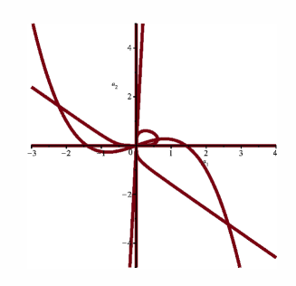
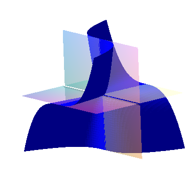
Figure 1. Left: Plot of the real part of the closed set defining $\Omega_{\mathrm{proper}(\mathcal{P})}$ in Example 5.10. Right: Plot of the real part of the closed set defining $\Omega_{\mathrm{genus}(F)}$ in Example 6.3

6. Decomposition of $\mathbb{S}$

The goal in this section is to provide an algorithm decomposing the space $\mathbb{S}$ so that in each subset of the decomposition we can give information on the genus of the corresponding specialized curve.

Let $F$ be as in (4.1), irreducible over $\overline{\mathbb{F}}$. We first compute the genus of $\mathcal{C}(F^{h})$. Let $\mathfrak{g}:=\mathrm{genus}(\mathcal{C}(F^{h}))$. Furthermore, if $\mathfrak{g}=0$, let $\mathcal{P}(\mathbf{a},\gamma,t)$ be, as in (5.1), a proper parametrization of $\mathcal{C}(F^{h})$. We consider the open subset

(6.1) $$\Sigma:=\left\{\begin{array}[]{cl}\Omega_{\mathrm{genus}(F)}&\text{if $\mathfrak{g}>0$ (see Def. \eqref{def-genus})}\\ \vspace*{1mm}\cr\Omega_{\mathrm{proper}(\mathcal{P})}&\text{if $\mathfrak{g}=0$ (see Def. \eqref{def-omega})}\end{array}\right.$$

At this level of the process we know that (see Theorems (4.13) and (5.5))

1. If $\mathfrak{g}>0$, then for $\mathbf{a}^{0}\in\Sigma$ it holds that $\mathcal{C}(F,\mathbf{a}^{0})$ is either reducible or its genus is $\mathfrak{g}$.

2. If $\mathfrak{g}=0$, then for $\mathbf{a}^{0}\in\Sigma$ it holds that $\mathcal{C}(F,\mathbf{a}^{0})$ is rational and $\mathcal{P}(\mathbf{a}^{0},\gamma^{0},t)$ parametrizes properly $\mathcal{C}(F,\mathbf{a}^{0})$.

In the following, we analyze the specializations when working in the closed set

(6.2) $$\mathcal{Z}:=\mathbb{S}\setminus\Sigma.$$

First, let us discuss the computational issues that may appear. Let $\mathcal{A}\subset\mathbb{K}[\mathbf{a}]$ be a set of generators of $\mathcal{Z}$, and let $\mathrm{I}$ be the ideal generated by $\mathcal{A}$ in $\mathbb{K}[\mathbf{a}]$. We consider the prime decomposition of $\mathrm{I}$

$$\mathrm{I}=\bigcup_{j=1}^{\ell}\mathrm{I}_{j}.$$

Now, for each prime ideal $\mathrm{J}\in\{\mathrm{I}_{1},\ldots,\mathrm{I}_{\ell}\}$ we consider the quotient field of $\mathbb{K}[\mathbf{a}]/\mathrm{J}$; we denote it by $\mathbb{L}_{\mathrm{J}}$. Elements in $\mathbb{L}_{\mathrm{J}}$ are quotients of equivalence classes of $\overline{\mathbb{K}}[\mathbf{a}]/\mathrm{J}$. We will assume that elements in $\overline{\mathbb{K}}[\mathbf{a}]/\mathrm{J}$ are always expressed by means of a canonical representative of the class in the following sense. We fix a Gröbner basis $\mathcal{G}$ of $\mathrm{J}$ w.r.t. some fixed order. Then, the elements in $\overline{\mathbb{K}}[\mathbf{a}]/\mathrm{J}$ are uniquely represented by their normal form w.r.t. $\mathcal{G}$ (see e.g. Prop. 1 and Ex. 13, Chap. 2, Sect. 6. in [6]) and, hence, elements in $\mathbb{L}_{\mathrm{J}}$ are represented as the quotient of the canonical representatives of their numerators and denominators. So, by abuse of notation, we will identify, via the canonical representation, the elements in $\mathbb{L}_{\mathrm{J}}$ with elements in $\overline{\mathbb{K}}(\mathbf{a})$. In addition, we consider an algebraic element $\gamma_{\mathrm{J}}$ over $\mathbb{L}_{\mathrm{J}}$ and we denote by $\mathbb{F}_{\mathrm{J}}$ the field $\mathbb{F}_{\mathrm{J}}:=\mathbb{L}_{\mathrm{J}}(\gamma_{\mathrm{J}})$.

We observe that $\mathbb{F}_{\mathrm{J}}$ is a computable field with a polynomial factorization algorithm available; zero test and basic arithmetic (addition, multiplication and inverse computation) can be carried out e.g. by taking the normal forms w.r.t. a Gröbner basis of $\mathrm{J}$. For the polynomial factorization we refer to (see Section 10.2 and Appendix B in [36], see also [35]). As a particular case, as in Example 5.10 and 6.2, if $\mathbb{V}(\mathrm{J})$ is a rational variety, one may work over $\mathbb{K}(\mathcal{Q}(\lambda_{1},\ldots,\lambda_{m}))$ instead of $\mathbb{F}_{\mathrm{J}}$, where $\mathcal{Q}(\lambda_{1},\ldots,\lambda_{m})$ is a parametrization of $\mathbb{V}(\mathrm{J})$.

Concerning specializations, instead of working in $\mathbb{S}$ (see (2.1)), we take the parameter values in the irreducible variety $\mathbb{V}(\mathrm{J})$. Then, for $\mathbf{a}^{0}\in\mathbb{V}(\mathrm{J})\subset\mathbb{S}$, and $f\in\overline{\mathbb{K}}[\mathbf{a}]/\mathrm{J}$, we denote by $f(\mathbf{a}^{0})$ the specialization at $\mathbf{a}^{0}$ of the equivalence class of $f$; note that since $\mathbf{a}^{0}\in\mathbb{V}(\mathrm{J})$ the specialization does not depend on the representative. Similarly, if $f:=p/q\in\mathbb{F}_{\mathrm{J}}$ and $q(\mathbf{a}^{0})\neq 0$, then $f(\mathbf{a}^{0}):=p(\mathbf{a}^{0})/q(\mathbf{a}^{0})\in\overline{\mathbb{K}}$.

In this situation, for each prime ideal $\mathrm{J}\in\{\mathrm{I}_{1},\ldots,\mathrm{I}_{\ell}\}$ we consider the polynomial $F$ in (4.1) as a polynomial in $\mathbb{F}_{\mathrm{J}}[x,y]$. To emphasize this fact, we write $F_{\mathrm{J}}$. First we check the irreducibility of $F_{\mathrm{J}}$ over the algebraic closure of $\mathbb{F}_{\mathrm{J}}$. If $F_{\mathrm{J}}$ is reducible we can either stop the decomposition over this closed subset, and claim that the specialization over $\mathbb{V}(\mathrm{J})$ is reducible, or continue the process with each irreducible factor of $F_{\mathrm{J}}$. For irreducible $F_{\mathrm{J}}$, the process continues, as in the initial step, by computing the genus of $\mathcal{C}(F_{\mathrm{J}})$. Since in each iteration of the process the dimension of the variety $\mathbb{V}(\mathrm{J})$ decreases, we, at the end, reach the zero–dimensional case, and the decomposition ends.

Let us say that a specialization degenerates if either $F(\mathbf{a}^{0},\gamma^{0},x,y)$ is not well–defined or $F(\mathbf{a}^{0},\gamma^{0},x,y)\in\overline{\mathbb{K}}$. As a result of the process described above, we find a disjoint decomposition

(6.3) $$\mathbb{S}=\dot{\bigcup}_{i\in I}\mathbb{S}_{i}$$

such that, for every specialization $\mathbf{a}^{0}\in\mathbb{S}_{i}$, one of the following holds

1. the specialization degenerates;

2. the genus is positive and preserved, or the specialized curve is reducible;

3. the genus is zero and a proper parametrization of $\mathcal{C}(F,\mathbf{a}^{0})$ is provided.

Remark 6.1.

Let us remark that in the decomposition (6.3) we can take the union of those $\mathbb{S}_{i}$ corresponding to each of the three items above; say $\mathbb{S}_{1},\mathbb{S}_{2},\mathbb{S}_{3}$ representing the corresponding item. In this way, we can achieve a unique decomposition of the parameter space $\mathbb{S}$. The $\mathbb{S}_{i}$ obtained in this way are constructible sets of $\mathbb{S}$, and $\mathbb{S}_{2},\mathbb{S}_{3}$ are a finite union of subsets $\Sigma$ as in (6.1) and $\mathbb{S}_{1}$ is a closed subset directly defined from the implicit equation $F$.

Moreover, $\mathbb{S}_{3}$ can further be decomposed into a finite union of subsets $\mathbb{S}_{3,j}$ such that for every $j$, there is a proper parametrization $\mathcal{P}_{j}$ which is well–defined for every $\mathbf{a}^{0}\in\mathbb{S}_{3,j}$ and specialized properly.

Finally, since $\Sigma$ of $F$ as in (6.1) is open on non-empty, depending on the genus of $F$, either $\mathbb{S}_{2}$ or $\mathbb{S}_{3}$ is a dense subset of $\mathbb{S}$.

We illustrate the previous ideas by continuing the analysis of Example 5.10.

Example 6.2.

(Continuation of Example 5.10) Taking into account (5.5), the closed set $\mathcal{Z}$ (see (6.2)) decomposes as

$$\mathcal{Z}=\mathbb{V}(a_{1})\cup\mathbb{V}(a_{2})\cup\mathbb{V}(a_{2}-27a_{1})\cup\mathbb{V}(a_{1}^{3}-2a_{1}+4a_{2})\cup\mathbb{V}(a_{1}^{5}+a_{2}^{5}+3a_{1}^{2}a_{2}^{2}-a_{1}a_{2})\subset\overline{\mathbb{Q}}^{2}.$$

We start with $\mathrm{J}_{1}:=<\!\!a_{1}\!\!>$ and $\mathbb{V}_{1}:=\mathbb{V}(\mathrm{J}_{1})$. Since $\mathbb{V}_{1}$ is rational, surjectively parametrized by $\mathcal{Q}_{1}:=(0,\lambda)$, we work over the field $\mathbb{Q}(\lambda)[x,y]$. We have that

$$F_{\mathrm{J}_{1}}:=\lambda^{2}x^{2}\left(\lambda^{3}x\,y^{2}-6\lambda^{2}xy+\lambda xy+9\lambda x-3x-2\right)$$

and therefore all specializations in $\mathbb{V}(a_{1})$ lead to a reducible curve. Additionally, one may distinguish the cases $\lambda=0$, that corresponds to the point $(0,0)$, where the specialization degenerates, and $\lambda\neq 0$ where $\mathcal{C}(F,\mathbf{a}^{0})$ decomposes to the union of a double line and a rational cubic.

The analysis for $\mathrm{J}_{2}:=<\!\!a_{2}\!\!>$, and $\mathbb{V}_{2}:=\mathbb{V}(\mathrm{J}_{2})$ looks similar. Since $\mathbb{V}_{2}$ is rational, parametrized by $\mathcal{Q}_{2}:=(\lambda,0)$, we work over the field $\mathbb{Q}(\lambda)[x,y]$. We have that

$$F_{\mathrm{J}_{2}}:=\, \lambda y(\lambda^{4}x^{3}y-6\lambda^{3}x^{2}y-\lambda^{3}x+2\lambda^{2}x^{2}+12\lambda^{2}xy-\lambda\,x^{3}-3\lambda^{3}+9\lambda^{2}x-9\lambda\,x^{2}+3x^{3}+2\lambda^{2}-4\lambda x-8\lambda y+2x^{2}).$$

Thus, all specializations in $\mathbb{V}_{2}$ lead to a reducible curve; note that $\mathcal{Q}_{2}$ is surjective. The case $\lambda=0$ is covered above, and for $\lambda\neq 0$, the specialization $\mathcal{C}(F,\mathbf{a}^{0})$ decomposes to the union of a line and a rational quartic.

Let us study $\mathrm{J}_{3}:=<\!\!a_{2}-27a_{1}\!\!>$ and $\mathbb{V}_{3}:=\mathbb{V}(\mathrm{J}_{3})$. Again, $\mathbb{V}_{3}$ is rational, parametrized by $\mathcal{Q}_{3}:=(\lambda,27\lambda)$, and we work over the field $\mathbb{Q}(\lambda)[x,y]$. We have that

$$F_{\mathrm{J}_{3}}:=\, \lambda(244\lambda x+3\lambda-3x-2)(58807\lambda^{3}x^{2}y^{2}-732\lambda^{3}x\,y^{2}+732\lambda^{2}x^{2}y^{2}+9\lambda^{3}y^{2}-13068\lambda^{2}x^{2}y$$

$$+464\lambda^{2}x\,y^{2}+9\lambda\,x^{2}y^{2}+81\lambda^{2}xy+6\lambda^{2}y^{2}-81\lambda\,x^{2}y-6\lambda x\,y^{2}-\lambda^{2}y+729\lambda\,x^{2}-106\lambda xy+4\lambda\,y^{2}-x^{2}y).$$

The analysis of $\mathbb{V}_{3}$ is identical to $\mathbb{V}_{2}$.

Let us study $\mathrm{J}_{4}:=<\!\!a_{1}^{3}-2a_{1}+4a_{2}\!\!>$ and $\mathbb{V}_{4}:=\mathbb{V}(\mathrm{J_{4}})$ that is again rational and it is properly and surjectively parametrized by $\mathcal{Q}_{4}:=(\lambda,-\frac{1}{4}\lambda^{3}+\frac{1}{2}\lambda)$. We work over the field $\mathbb{Q}(\lambda)[x,y]$. We have that

$$F_{\mathrm{J}_{4}}:=\, \lambda(\lambda^{5}y-2\lambda^{3}y+12\lambda^{2}-8\lambda+32y)(\lambda^{9}x^{3}y-8\lambda^{7}x^{3}y+12\lambda^{6}x^{3}+24\lambda^{5}x^{3}y+8\lambda^{5}x^{3}-32\lambda^{4}x^{3}y$$

$$-72\lambda^{4}x^{3}-32\lambda^{3}x^{3}y-16\lambda^{4}x^{2}-32\lambda^{3}x^{3}+192\lambda^{3}x^{2}y+144\lambda^{2}x^{3}+16\lambda\,x^{3}y+64\lambda^{2}x^{2}-384\lambda^{2}xy$$

$$+32\lambda\,x^{3}-96x^{3}+256\lambda y-64x^{2}).$$

Again $\mathbb{V}_{4}$ behaves as $\mathbb{V}_{2}$ and $\mathbb{V}_{3}$. Finally, let us analyze $\mathrm{J}_{5}:=<\!\!a_{1}^{5}+a_{2}^{5}+3a_{1}^{2}a_{2}^{2}-a_{1}a_{2}\!\!>$ and $\mathbb{V}_{5}:=\mathbb{V}(\mathrm{J}_{5})$ which is a rational quintic and properly and surjectively parametrized as

$$\mathcal{Q}_{5}(\lambda):=\left({\frac{\left(5\,\lambda-1\right)\left(5\,\lambda-2\right)^{4}}{3125\,{\lambda}^{4}-3750\,{\lambda}^{3}+1750\,{\lambda}^{2}-375\,\lambda+31}},-{\frac{\left(5\,\lambda-2\right)\left(5\,\lambda-1\right)^{4}}{3125\,{\lambda}^{4}-3750\,{\lambda}^{3}+1750\,{\lambda}^{2}-375\,\lambda+31}}\right).$$

Those values for which the parametrization is not defined, i.e. the poles, play no role in this analysis. The polynomial $F_{\mathrm{J}_{5}}$ is $F_{\mathrm{J}_{5}}(\lambda,x,y)=F(\mathcal{Q}_{5}(\lambda),x,y)\in\mathbb{Q}(\lambda)[x,y]$. It holds that $\deg(\mathcal{C}(F_{\mathrm{J}_{5}}))=4$, $\mathrm{genus}(\mathcal{C}(F_{\mathrm{J}_{5}}))=0$ and a proper surjective parametrization is $\mathcal{P}_{\mathrm{J}_{5}}(\lambda,t):=\mathcal{P}(\mathcal{Q}(\lambda),t)$ (see (5.4)). So, we get (see Def. 5.4)

$$\Omega_{\mathrm{proper}(\mathcal{P}_{\mathrm{J}_{5}})}:=\mathbb{V}_{5}\setminus\{\mathcal{P}_{\mathrm{J}_{5}}(\lambda_{0})\,|\,f(\lambda_{0})=0\}$$

where $f:=p_{1}\,p_{2}\,p_{3}\,p_{4}$ and

$$\begin{array}[]{ll}p_{1}:=&5\,\lambda-1,\,\,\,p_{2}:=5\,\lambda-2,\,\,\,p_{3}:=25\,{\lambda}^{2}-15\,\lambda+3,\\ p_{4}:=&\text{\small{$390625\,{\lambda}^{8}-937500\,{\lambda}^{7}+1343750\,{\lambda}^{6}-1237500\,{\lambda}^{5}+711875\,{\lambda}^{4}-253500\,{\lambda}^{3}$}}\\ &\text{\small{$+54475\,{\lambda}^{2}-6495\,\lambda+331.$}}\end{array}$$

By Theorem 5.5, for every $\mathbf{a}^{0}\in\Omega_{\mathrm{proper}(\mathcal{P}_{\mathrm{J}_{5}})}$ it holds that $\mathcal{C}(F,\mathbf{a}^{0})$ is rationally parametrized by $\mathcal{P}(\mathbf{a}^{0},t)$ (see (5.4)) or, equivalently, by $\mathcal{P}_{\mathrm{J}_{5}}(\mathcal{Q}^{-1}(\mathbf{a}^{0}),t)$. Now, let us analyze the curve in $\mathcal{Z}_{5}:=\mathbb{V}_{5}\setminus\Omega_{\mathrm{proper}(\mathcal{P}_{\mathrm{J}_{5}})}=\{\mathcal{P}_{\mathrm{J}_{5}}(\lambda_{0})\,|\,f(\lambda_{0})=0\}$ (see (6.2)). We define $\mathbf{a}^{0}_{1}:=(0,0)=\mathcal{P}_{\mathrm{J}_{5}}(\lambda_{0})$, where $\lambda_{0}$ is a root of $p_{1}\,p_{2}$; $\mathbf{a}^{0}_{2}:=(-1,-1)=\mathcal{P}_{\mathrm{J}_{5}}(\lambda_{0})$, where $\lambda_{0}$ is a root of $p_{3}$; and observe that $p_{4}$ generates 8 points on the curve that we denote by $\mathbf{a}^{0}_{i},i\in\{3,\ldots,10\}$ and which correspond to $\mathcal{P}_{\mathrm{J}_{5}}(\lambda_{0})$ where $\lambda_{0}$ is one of the roots of $p_{4}$. Thus, $\mathcal{Z}=\{\mathbf{a}^{0}_{1},\ldots,\mathbf{a}^{0}_{10}\}$, $\mathcal{C}(F,\mathbf{a}^{0}_{1})=\mathbb{C}^{2}$, and, for $i\in\{2,\ldots,10\}$, $\mathcal{C}(F,\mathbf{a}^{0}_{i})$ are rational cubics parametrized by $\mathcal{P}_{\mathrm{J}_{5}}(\mathbf{a}^{0}_{i},t)$.

Summarizing, $\mathbb{S}$ decomposes as (see (6.3) and Remark 6.1)

$$\mathbb{S}= \left(\mathbb{S}_{1}:=\{(0,0)\}\right)\cup\left(\mathbb{S}_{2}:=\cup_{i=1}^{4}\mathbb{V}_{i}\setminus\{(0,0)\}\right)$$

$$\cup\left(\mathbb{S}_{3,1}:=\Omega_{\mathrm{proper}(\mathcal{P})}\right)\cup\left(\mathbb{S}_{3,2}:=\Omega_{\mathrm{proper}(\mathcal{P}_{\mathrm{J}_{5}})}\right)\cup\left(\mathbb{S}_{3,3}:=\{\mathbf{a}^{0}_{2},\ldots,\mathbf{a}^{0}_{10}\}\right).$$

For $\mathbf{a}^{0}\in\mathbb{S}_{1}$, $\mathcal{C}(F,\mathbf{a}^{0})$ degenerates. For $\mathbf{a}^{0}\in\mathbb{S}_{2}$, $\mathcal{C}(F,\mathbf{a}^{0})$ is reducible (note that $\mathbf{a}^{0}_{1}\in\mathbb{S}_{2}$). For $\mathbf{a}^{0}\in\mathbb{S}_{3,1}$, the specialized curve $\mathcal{C}(F,\mathbf{a}^{0})$ is a quintic parametrized by $\mathcal{P}(\mathbf{a}^{0},t)$; for $\mathbf{a}^{0}\in\mathbb{S}_{3,2}$, $\mathcal{C}(F,\mathbf{a}^{0})$ is a quartic parametrized by $\mathcal{P}_{\mathrm{J}_{5}}(\mathbf{a}^{0},t)$; and for $\mathbf{a}^{0}\in\mathbb{S}_{3,3}$, $\mathcal{C}(F,\mathbf{a}^{0})$ is a cubic parametrized by $\mathcal{P}_{\mathrm{J}_{5}}(\mathbf{a}^{0},t)$.

Example 6.3.

Let $\mathbb{K}=\mathbb{Q}$ and $\mathbb{F}=\mathbb{L}=\mathbb{Q}(a_{1},a_{2},a_{3})$. We consider

$$F={x}^{3}+{x}^{2}a_{{1}}+{y}^{3}+a_{{2}}a_{{3}}\in\mathbb{F}[x,y].$$

One has that $\mathrm{genus}(\mathcal{C}(F))=1$. Using the ideas in Section 4, we compute $\Omega_{\mathrm{genus}(F)}$ (see Def. 4.12). We observe that since $\mathcal{C}(F)$ is an elliptic cubic, no blowup is required and, hence, $\Omega_{\mathrm{genus}(F)}=\Omega_{\mathrm{genusOrd}(F)}$. Indeed, one gets that (see Fig. 1, right)

$$\Omega_{\mathrm{genus}(F)}:=\mathbb{C}^{3}\setminus\mathbb{V}\left(-a_{{2}}a_{{3}}\left(-4\,{a_{{1}}}^{3}-27\,a_{{2}}a_{{3}}\right)\right).$$

Thus, by Theorem 4.8, for every $\mathbf{a}^{0}\in\Omega_{\mathrm{genus}(F)}$, $\mathcal{C}(F,\mathbf{a}^{0})$ is either reducible or it is a genus 1 cubic curve. Let us analyze the specializations in $\mathcal{Z}:=\mathbb{C}^{3}\setminus\Omega_{\mathrm{genus}(F)}=\mathbb{V}\left(-a_{{2}}a_{{3}}\left(-4\,{a_{{1}}}^{3}-27\,a_{{2}}a_{{3}}\right)\right)$.

Let $\mathrm{J}_{1}:=<\!\!a_{2}\!\!>$ and $\mathbb{V}_{1}:=\mathbb{V}(\mathrm{J}_{1})$. Then, $F_{\mathrm{J}_{1}}:={x}^{3}+a_{{1}}{x}^{2}+{y}^{3}$. We observe that $\mathrm{genus}(\mathcal{C}(F_{\mathrm{J}_{1}}))=0$ and

$$\mathcal{P}_{\mathrm{J}_{1}}:=\left(-{\frac{{t}^{3}a_{{1}}}{{t}^{3}+1}},-{\frac{{t}^{2}a_{{1}}}{{t}^{3}+1}}\right)$$

is a proper parametrization of $\mathcal{C}(F_{\mathrm{J}_{1}})$. Applying Def. 5.4 to $F_{\mathrm{J}_{1}}$ and $\mathcal{P}_{\mathrm{J}_{1}}$ we get that $\Omega_{\mathrm{proper}(\mathcal{P}_{\mathrm{J}_{1}})}:=\mathbb{V}_{1}\setminus\mathbb{V}(a_{1})$. Therefore, by Theorem 5.5, for all $\mathbf{a}^{0}\in\Omega_{\mathrm{proper}(\mathcal{P}_{\mathrm{J}_{1}})}$ it holds that $\mathcal{C}(F,\mathbf{a}^{0})$ is a rational curve parametrized by $\mathcal{P}_{\mathrm{J}_{1}}(\mathbf{a}^{0},t)$. However, for the remaining case, namely the points $(0,0,\mu)$ for $\mu\in\mathbb{C}$, $\mathcal{C}(F,(0,0,\mu))$ decomposes as the product of three lines.

Let $\mathrm{J}_{2}:=<\!\!a_{3}\!\!>$ and $\mathbb{V}_{2}:=\mathbb{V}(\mathrm{J}_{2})$. Now, the situation is identical to the previous case. Let $\mathrm{J}_{3}:=<\!\!-4\,{a_{{1}}}^{3}-27\,a_{{2}}a_{{3}}\!\!>$ and $\mathbb{V}_{3}:=\mathbb{V}(\mathrm{J}_{3})$. The surface $\mathbb{V}_{3}$ can be properly parametrized as

$$\mathcal{Q}(\lambda_{1},\lambda_{2})=\left(\lambda_{{1}},\lambda_{{2}},-{\frac{4\,{\lambda_{{1}}}^{3}}{27\,\lambda_{{2}}}}\right).$$

We observe that $\mathcal{Q}$ is not surjective. Indeed, $\mathcal{Q}(\mathbb{C}^{2})=\mathbb{V}_{3}\setminus\{(0,0,\mu)\,|\,\mu\in\mathbb{C}\}$ (see e.g. Remark 3 in [26]). However, the specializations in $\{(0,0,\mu)\,|\,\mu\in\mathbb{C}\}$ have already been analyzed. So, we treat the case $\mathcal{Q}(\mathbb{C}^{2})$. Then, $F_{\mathrm{J}_{3}}$ can be taken as

$$F_{\mathrm{J}_{3}}:=F(\mathcal{Q}(\lambda_{1},\lambda_{2}),t)={x}^{3}+{x}^{2}\lambda_{{1}}+{y}^{3}-{\frac{4\,{\lambda_{{1}}}^{3}}{27}},$$

where $(\lambda_{1},\lambda_{2})\in\mathbb{C}^{2}\setminus\{(0,0)\}$. It holds that $\mathrm{genus}(\mathcal{C}(F_{\mathrm{J}_{3}}))=0$ and

$$\mathcal{P}_{\mathrm{J}_{3}}:=\left({\frac{{t}^{3}\lambda_{{1}}-2\,\lambda_{{1}}}{3\,{t}^{3}+3}},{\frac{{t}^{2}\lambda_{{1}}}{{t}^{3}+1}}\right)$$

is a proper parametrization. Applying Def. 5.4 to $F_{\mathrm{J}_{3}}$ and $\mathcal{P}_{\mathrm{J}_{3}}$, we get that $\Omega_{\mathrm{proper}(\mathcal{P}_{\mathrm{J}_{3}})}=\mathbb{V}_{3}\setminus\{(0,0,\mu)\,|\,\mu\in\mathbb{C}\}$. Therefore, by Theorem 5.5, for all $\mathbf{a}^{0}\in\Omega_{\mathrm{proper}(\mathcal{P}_{\mathrm{J}_{3}})}$ it holds that $\mathcal{C}(F,\mathbf{a}^{0})$ is a rational curve parametrized by $\mathcal{P}_{\mathrm{J}_{3}}(\mathbf{a}^{0},t)$.

Summarizing, $\mathbb{S}$ decomposes as (see (6.3))

$$\mathbb{S}=\left(\mathbb{S}_{2}:=\Omega_{\mathrm{genus}(F)}\cup\{(0,0,\mu)\,|\,\mu\in\mathbb{C}\}\right)\cup\left(\mathbb{S}_{3}:=\Omega_{\mathrm{proper}(\mathcal{P}_{\mathrm{J}_{1}})}\right).$$

For $\mathbf{a}^{0}\in\mathbb{S}_{2},\mathcal{C}(F,\mathbf{a}^{0})$ is either reducible or an elliptic curve; and for $\mathbf{a}^{0}\in\mathbb{S}_{3},\mathcal{C}(F,\mathbf{a}^{0})$ is a rational cubic parametrized by $\mathcal{P}_{\mathrm{J}_{3}}(\mathbf{a}^{0},t)$.

7. Some Illustrating Applications

In this section, we illustrate by examples some possible applications of the theory developed in the paper. In the first example, given a surface, we consider the problem of determining its rational level curves, if any.

Example 7.1.

Level curves of a surface.
Let $\mathcal{S}$ be the surface defined over $\mathbb{C}$ by the polynomial

$$F=x^{6}-5x^{4}y+3x^{4}z-y^{5}+2y^{4}z-y^{3}z^{2}-x^{3}z+5x^{2}y^{2}-7x^{2}yz+3x^{2}z^{2}+y^{2}z-2yz^{2}+z^{3}-x^{2}$$

where $F\in\mathbb{Q}(z)[x,y]$. So, with the terminology of the paper, $\mathbf{a}=z$, $\mathbb{K}=\mathbb{Q}$ and $\mathbb{L}=\mathbb{F}=\mathbb{Q}(z)$. With this interpretation, the idea is to analyze the genus of $\mathcal{C}(F)\subset\overline{\mathbb{Q}(z)}^{2}$ under specializations in $\mathbb{S}:=\mathbb{C}$. For this purpose, we first compute a standard decomposition of the singular locus as in (4.2). Following the steps described in Subsection A.1, we get

$$\mathscr{F}(F^{h})=\left\{\left(0:z:1\right)\right\}_{m_{1}=t}.$$

Moreover, one can easily check that the family consists in one ordinary double point. Therefore, one gets that $\mathrm{genus}(\mathcal{C}(F))=9$. Since the singularities are all ordinary, we get that (see Def. 4.12) $\Omega_{\mathrm{genus}(F)}=\Omega_{\mathrm{genusOrd}(F)}.$ Moreover (see Def. 4.5),

$$\begin{array}[]{ll}\Omega_{\mathrm{genusOrd}(F)}=&\mathbb{C}\setminus\left\{-1,0,1\right\}.\end{array}$$

Using Theorem 4.13, for $z_{0}\in\Omega_{\mathrm{genusOrd}(F)}$, $\mathcal{C}(F,(x,y,z_{0}))$ is either reducible or its genus is 9. In any case, no rational level curve appears. For the elements in $\mathcal{Z}:=\mathbb{C}\setminus\Omega_{\mathrm{genusOrd}(F)}$, we get that $\mathcal{C}(F,(x,y,\pm 1))$ are irreducible of genus 7 and $\mathcal{C}(F,(x,y,0))$ is irreducible of genus 0. Indeed, $\mathcal{C}(F,(x,y,0))$ can be parametrized by $(t^{5},t^{6}-t^{2})$.

In the second example, we consider the linear homotopy deformation of two curves and we analyze the genus of each instance curve.

Example 7.2.

Linear homotopy deformation of curves.
Let us consider the linear homotopy between the Fermat cubic curve and the unit circle. That is we consider the polynomial

$$F=\left(1-\lambda\right)\left(x^{3}+y^{3}-1\right)+\lambda\left(x^{2}+y^{2}-1\right).$$

We consider $F$ as a polynomial in $\mathbb{Q}(\lambda)[x,y]$ and we analyze the genus behavior through the deformation. So, with the terminology of the paper, $\mathbf{a}=\lambda$, $\mathbb{K}=\mathbb{Q}$ and $\mathbb{L}=\mathbb{F}=\mathbb{Q}(\lambda)$. Now, the idea is to study the genus of $\mathcal{C}(F)$ under specializations in $\mathbb{S}:=\mathbb{C}$; or, in particular, in the real interval $[0,1]$. For this purpose, we first observe that $\mathrm{genus}(\mathcal{C}(F))=1$ and hence (see Def. 4.12), $\Omega_{\mathrm{genus}(F)}=\Omega_{\mathrm{genusOrd}(F)}.$ We get that $\Omega_{\mathrm{genusOrd}(F)}=\mathbb{C}\setminus\mathbb{V}(g)$ where

$$g(\lambda)= -\left(2\lambda^{3}-5\lambda^{2}+7\lambda-3\right)\left(\lambda^{6}-4\lambda^{5}+15\lambda^{4}-29\lambda^{3}+43\lambda^{2}-33\lambda+9\right)\left(4\lambda-3\right)\left(-1+\lambda\right)\left(\lambda-3\right)$$

$$\left(2\lambda^{9}+27\lambda^{8}+5049\lambda^{7}-40068\lambda^{6}+148716\lambda^{5}-315657\lambda^{4}+398763\lambda^{3}-295245\lambda^{2}+118098\lambda-19683\right)$$

$$\left(8\lambda^{3}-27\lambda^{2}+54\lambda-27\right).$$

Using Theorem 4.13, for $\lambda_{0}\in\Omega_{\mathrm{genusOrd}(F)}$, $\mathcal{C}(F,(x,y,\lambda_{0}))$ is either reducible or its genus is 1. In any case, no rational deformation instance appears. For the elements in $\mathcal{Z}=\mathbb{C}\setminus\Omega_{\mathrm{genusOrd}(F)}$, we get that $\mathcal{C}(F,(x,y,1))$ is rational, the specialized cubics $\mathcal{C}(F,(x,y,3/4))$ and $\mathcal{C}(F,(x,y,3))$ factor as a union of a line and a conic, and for all the other cases the genus remains one (see Fig 2).

Figure 2. Left: Plot of the real part of different instances of the deformation in Example 7.2. Right: Plot of the real part of $\mathcal{C}(F,(x,y,3/4))$ and $\mathcal{C}(F,(x,y,3))$ in Example 7.2.

Let $\mathcal{O}$ be a connected open subset of $\mathbb{C}$ and let $\mathrm{Mer}(\mathcal{O})$ be the field of meromorphic functions in $\mathcal{O}$ (see [14]). We consider a polynomial equation of the form

(7.1) $$\sum_{i,j\in{I}}f_{i,j}(t)x^{i}y^{j}=0$$

where $I$ is a finite subset of $\mathbb{N}^{2}$, and where $f_{i,j}\in\mathrm{Mer}(\mathcal{O})$. Let $\mathbf{f}$ be the tuple with all the functions $f_{i,j}$ appearing in (7.1). The question now is to decide, and indeed compute, whether there exists rational solutions of the equation; that is $p,q\in\overline{\mathbb{C}(\mathbf{f})}$ such that $\sum_{i,j\in{I}}f_{i,j}(t)p^{i}q^{j}=0$.

We may proceed as follows. We consider the polynomial $F(\mathbf{a},x,y)$ resulting from the formal replacement in (7.1) of each function $f_{i,j}$ by a parameter $a_{k}$. Now, with the terminology of the paper, we take $\mathbb{K}=\mathbb{C}(\mathbf{f})$ and $\mathbb{L}=\mathbb{F}=\mathbb{K}(\mathbf{a})$.

Then, we decompose $\mathbb{S}$ (see (2.1)) as described in Section 6; note that the computations can be carried out over $\mathbb{C}(\mathbf{a})$ instead of over $\mathbb{F}$. Then, if any subset in the decomposition has genus zero, and the functions $\mathbf{f}$ belong to it, we obtain a (family of) rational solutions. Let us see a particular example.

Example 7.3.

Rational solution of functional algebraic equations.
We consider the functional algebraic equation

(7.2) $$x^{2}y^{3}f_{1}^{4}-x^{2}y^{2}f_{2}^{4}f_{3}-2x\,y^{3}f_{1}^{2}f_{2}+2xyf_{1}f_{2}^{2}f_{3}^{2}+y^{3}f_{2}^{2}-f_{1}^{2}f_{3}^{3}=0,$$

where $\mathbf{f}=(f_{1},f_{2},f_{3}):=(\sin(t),\cos(t),\mathrm{e}^{t})$. We associate to (7.2) the curve $\mathcal{C}(F)$ where

$$F=x^{2}y^{3}a_{1}^{4}-x^{2}y^{2}a_{2}^{4}a_{3}-2x\,y^{3}a_{1}^{2}a_{2}+2xya_{1}a_{2}^{2}a_{3}^{2}+y^{3}a_{2}^{2}-a_{1}^{2}a_{3}^{3}.$$

It holds that $\mathrm{genus}(\mathcal{C}(F))=0$ and that a proper parametrization is

(7.3) $$\mathcal{P}(\mathbf{a},W)=\left(\frac{W^{3}a_{1}+a_{2}}{Wa_{2}^{2}+a_{1}^{2}},\frac{a_{3}}{W^{2}}\right).$$

The open subset in Def. 5.4 turns to be

$$\Omega_{\mathrm{proper}(\mathcal{P})}=\overline{\mathbb{C}(\mathbf{f})}^{3}\setminus\mathbb{V}_{\overline{\mathbb{C}(\mathbf{f})}}\left(a_{1}a_{2}\left(a_{1}-a_{2}\right)\left(a_{1}^{6}+a_{1}^{5}a_{2}+a_{1}^{4}a_{2}^{2}+a_{1}^{3}a_{2}^{3}+a_{1}^{2}a_{2}^{4}+a_{1}a_{2}^{5}+a_{2}^{6}\right)a_{3}\right).$$

Since $\mathbf{f}\in\Omega_{\mathrm{proper}(\mathcal{P})}$, by Theorem 5.5, we have that

(7.4) $$\left\{x=\frac{W^{3}\sin\!\left(t\right)+\cos\!\left(t\right)}{W\left(\cos^{2}\left(t\right)\right)+\sin^{2}\left(t\right)},y=\frac{{\mathrm{e}}^{t}}{W^{2}}\right\},$$

for every $W\in\overline{\mathbb{C}(\mathbf{f})}$ such that (7.4) is well–defined, is a rational solution of (7.2). In fact, the last statement holds more generally for every $W\in\overline{\mathrm{Mer}(\mathbb{C})}$.

Appendix A Rational Curves

In this appendix we recall the main steps to compute the genus of an irreducible plane curve and, in the affirmative case, how to parametrize a proper rational curve. There exist different methods to that goal: the adjoint curve based method (see e.g. [37] and [30]), the method based on the anticanonical divisor (see [13]) or the method based on Puiseux expansions (see [20]), among others. In this paper we will follow the adjoint curve based method (see [37]); more precisely, we will follow the symbolic approaches in Chapters 3,4,5 in [30]. A similar treatment of the problem can be performed using the other algorithmic approaches.

Throughout this appendix, let $G\in K[x,y]\setminus K$ be irreducible over $\overline{K}$.

A.1. Genus computation

We denote the genus as either $\mathrm{genus}(\mathcal{C}(G))$ or $\mathrm{genus}(\mathcal{C}(G^{h}))$. The key tool for our symbolic computation of the genus is the notion of conjugate family of points (see Definition 3.15 in [30]). We adapt the definition to our purposes.

Definition A.1.

The set $\mathcal{F}=\{(f_{1}(\alpha):f_{2}(\alpha):f_{3}(\alpha))\,|\,m(\alpha)=0\}\subset\mathbb{P}^{2}(\overline{K})$ is called a $K$–conjugate family of points if

1. at least one of the polynomials $f_{i}$ is not zero,

2. $f_{1},f_{2},f_{3},m\in K[t]$ and $gcd(f_{1},f_{2},f_{3},m)=1$,

3. $\deg_{t}(m)>0$ and $m$ is squarefree.

The family is represented as

$$\mathcal{F}:=\{(f_{1}(t):f_{2}(t):f_{3}(t))\}_{m(t)}$$

and $m(t)$ is called the defining polynomial of $\mathcal{F}$. We say that $\mathcal{F}$ is a family of points of $\mathcal{C}(G^{h})$ if $G^{h}(f_{1},f_{2},f_{3})=0$ modulo $m$. If $m(t)$ is irreducible over $K$, we say that $\mathcal{F}$ is irreducible.

Remark A.2.

1. We will assume that families are always represented in canonical form. That is, if $\mathcal{F}:=\{(f_{1}(t):f_{2}(t):f_{3}(t))\}_{m(t)}$ then $f_{1},f_{2},f_{3}$ are reduced modulo $m(t)$.

2. Note that a single point $(a:b:c)\in\mathbb{P}^{2}(K)$ can be seen as a $K$-conjugate family, for instance as $\{(a:b:c)\}_{t}.$

3. Note that, factoring the defining polynomial $m(t)$ over $K$, every family decomposes as a finite union of irreducible families. So, in general, we may assume that families are irreducible. Observe that, for $H\in K[x,y,z]$ and $\mathcal{F}:=\{(f_{1}(t):f_{2}(t):f_{3}(t))\}_{m(t)}$ irreducible, $H(f_{1},f_{2},f_{3})\neq 0$ mod $m(t)$ iff $H$ does not vanish at any point in the family $\mathcal{F}$. Moreover, if $\mathcal{F}$ is irreducible, then $K_{m}:=K[t]/\!<\!m\!>$ is an integral domain, and we can see $(f_{1}(t):f_{2}(t):f_{3}(t))$ as a single point in the curve defined by $G^{h}$ over $\overline{K_{m}}$. Let us denote this curve by $\mathcal{C}(G^{h}_{\mathcal{F}})$. In that situation, by abuse of notation, we will say that $\mathcal{F}$ is a point of $\mathcal{C}(G^{h}_{\mathcal{F}})$ meaning that $(f_{1}(t):f_{2}(t):f_{3}(t))\in\mathcal{C}(G^{h}_{\mathcal{F}})$.

In [30] it is proved that the singular locus of $\mathcal{C}(G^{h})$ can be decomposed as a finite union of irreducible families of $K$-conjugate points such that in each family the multiplicity and the singularity character (i.e. whether the singularity is ordinary or non–ordinary) is preserved. The set of all conjugate families appearing in the union above is called a $K$–standard decomposition of the singular locus of $\mathcal{C}(G^{h})$, or of $\mathcal{C}(G)$. In the following, we describe a process to determine a $K$–standard decomposition of the singular locus; see also [30] page 83. First, we introduce the notion of regular position:

Definition A.3.

We say that the affine plane curve $\mathcal{C}(G)$ is in regular position w.r.t. $x$ if

1. the coefficient of $y^{\deg(G)}$ in $G$ is a non-zero constant; and

2. $G(a,b_{i})=G_{x}(a,b_{i})=0$ with $i\in\{1,2\}$ implies that $b_{1}=b_{2}$.

If $\mathcal{C}(G)$ is not in regular position, we may apply a linear change of coordinates over $\mathbb{K}$ such that $G$ is transformed into regular position (see e.g. Lemma 2 in [10]). More precisely, for this purpose, one may perform a change of coordinates of the form $\{x=\bar{x}+q\bar{y},y=\bar{y}\}$ where $q$ is taken in an open subset defined by means of subresultants and by the homogeneous component of maximum degree in $G$ (see e.g. Remark 3 in [10]).

Condition (1) in Definition (A.3) is easy to check. Let us now deal with the second condition. Let us consider the ideal $\mathrm{J}$ generated by $\{G,G_{x}\}$ in $K[x,y]$. Taking into account that $G$ is irreducible over $\overline{K}$, one has that $\mathrm{J}$ is zero–dimensional. Therefore, using the Shape lemma (see [39] page 194), the normed reduced Gröbner basis of $\sqrt{\mathrm{J}}$, w.r.t. the lexicographic order $x<y$, is of the form

$$\{u(x),y-v(x)\},$$

with $u$ square-free and $\deg(v)<\deg(u)$, if and only if $\sqrt{\mathrm{J}}$, or equivalently $\mathrm{J}$, satisfies condition (2) in Definition (A.3). It remains to have a computational approach to determine $\sqrt{\mathrm{J}}$. This can be achieved, for instance, using Seidenberg lemma (see e.g. [22] or [15]). More precisely, if $\mathrm{J}\cap K[x]=<\!f(x)\!>$ and $\mathrm{J}\cap K[y]=<\!g(y)\!>$, then

(A.1) $$\sqrt{\mathrm{J}}=<\!G,G_{x},\tilde{f},\tilde{g}\!>,$$

where $\tilde{f}=f/\gcd(f,f^{\prime})$ and $\tilde{g}=g/\gcd(g,g^{\prime})$ and where $f^{\prime}$ and $g^{\prime}$ denotes the derivatives of $f$ and $g$ w.r.t. $x$ and $y$, respectively.

Then, the process for computing a standard decomposition of the singular locus of $\mathcal{C}(G^{h})$ is as follows.

Standard decomposition of the singular locus

Step 1: Regular position. If $\mathcal{C}(G)$ is not in regular position, apply an affine linear change of coordinates over $\mathbb{K}$, say $\mathcal{L}$, such that $\mathcal{C}(G)$ is transformed into regular position (see comments above).

Step 2: Families of singularities at infinity. Factor $G^{h}(x,y,0)$ over $K$,

$$G^{h}(x,y,0)=\prod_{i\in I}g_{i}(x,y)^{e_{i}}.$$

Note that none of the polynomials $g_{i}$ is $x$ because $\mathcal{C}(G)$ is in regular position w.r.t. $x$. Then, the set of points at infinity decomposes in irreducible $K$–conjugate families as

$$\bigcup_{i\in I}\{(1:t:0)\}_{g_{i}(1,t)}.$$

Now, a family $\{(1:t:0)\}_{g_{i}(1,t)}$ is singular if and only if $G^{h}_{x}(1,t,0)=G^{h}_{y}(1,t,0)=G^{h}_{z}(1,t,0)=0$ modulo $g_{i}(1,t)$. Let $\mathcal{I}$ be the set containing all $g_{i}(1,t)$ defining singularities. Then, the irreducible families of $K$–conjugate singularities at infinity are

(A.2) $$\bigcup_{m\in\mathcal{I}}\{(1:t:0)\}_{m(t)}.$$

Step 3: Families of affine singularities. Let $\mathrm{I}$ be the ideal generated by $\{G,G_{x},G_{y}\}$. Since $\sqrt{\mathrm{I}}$ is regular w.r.t. $x$ because of condition (2) in Def. A.3, and zero–dimensional, by the discussion above on the Shape lemma, the normed reduced Gröbner basis w.r.t. the lexicographic order with $x<y$ of $\sqrt{\mathrm{I}}$ is of the form $\{A(x),y-B(x)\}$ with $A$ square-free and $\deg(B)<\deg(A)$; recall that if $\mathrm{I}\cap K[x]=<\!f(x)\!>$ and $\mathrm{I}\cap K[y]=<\!g(y)\!>$, then

$$\sqrt{\mathrm{I}}=<\!G,G_{x},G_{y},\tilde{f},\tilde{g}\!>,$$

where $\tilde{f}=f/\gcd(f,f^{\prime})$, $\tilde{g}=g/\gcd(g,g^{\prime})$, and $f^{\prime}$ and $g^{\prime}$ denote the derivatives of $f$ and $g$ w.r.t. $x$ and $y$, respectively. So, each irreducible factor $m(x)$ of $A(x)$ over $K$ generates the irreducible family $\{(t:B(t):1)\}_{m(t)}.$ Therefore, if $\mathcal{A}$ denotes the set of all irreducible factors of $A$, the affine singularities decompose in irreducible $K$–families as

(A.3) $$\bigcup_{a\in\mathcal{A}}\{(t:B(t):1)\}_{m(t)}.$$

Step 4: Standard decomposition. Applying $\mathcal{L}^{-1}$ to (A.2) and to (A.3) we get an $K$–standard decomposition of the singular locus of $\mathcal{C}(G^{h})$. We observe that the irreducible families of affine singularities will be of the form $\{(f_{1}(t):f_{2}(t):1)\}_{m(t)}$ and the singularities at infinity of the form $\{(L_{1}(t):L_{2}(t):0)\}_{m(t)}$ with $\deg_{t}(L_{i})\leq 1$ and $\gcd(L_{1},L_{2})=1$.

Let $\mathscr{F}$ be a $K$–standard decomposition of the singular locus of $\mathcal{C}(G^{h})$ and let $\mathcal{F}\in\mathscr{F}$; note that by construction, $\mathcal{F}$ is irreducible. Then, we denote by $\mathrm{mult}(\mathcal{F})$ the multiplicity of the points in $\mathcal{F}$, as points of $\mathcal{C}(G^{h})$. In addition, since the character of the singularity is invariant within the family we will speak about ordinary and non-ordinary families. The multiplicity of an irreducible family $\mathcal{F}=\{(f_{1}:f_{2}:f_{3})\}_{m(t)}$ can be computed by determining the greatest non-negative integer $r$ such that all partial derivatives of $G^{h}$ of order less than $r$ vanish at $(f_{1}:f_{2}:f_{3})$ modulo $m(t)$. The character of $\mathcal{F}$ can be decided by analyzing the squarefreeness, modulo $m(t)$, of the polynomial defining the tangents to $\mathcal{C}(G^{h})$ at $(f_{1}:f_{2}:f_{3})$. Alternatively, one can work with the curve $\mathcal{C}(G^{h}_{\mathcal{F}})$ (see Remark A.2 (3)). Now, the family $\mathcal{F}$ in $\mathcal{C}(G^{h})$ turns to be one point in $\mathcal{C}(G^{h}_{\mathcal{F}})$, namely $(f_{1}:f_{2}:f_{3})$. Then, the character and multiplicity of $\mathcal{F}$ is the character and multiplicity of $(f_{1}:f_{2}:f_{3})$ as a point in $\mathcal{C}(G^{h}_{\mathcal{F}})$.

Once the singularities have been detected, one proceeds to recursively, and separately, blow up each non–ordinary singularity via the neighboring singularities (see [37] or [30] for more details). Let us briefly recall how the first iteration step works, first for a single point, and afterwards for an irreducible family of conjugate points. In the following, let $p\in\mathcal{C}(G^{h})$ be a non–ordinary singular point.

Blow up basic step

Step 1. Apply a linear change of coordinates $\mathcal{L}$ such that: $p=\mathcal{L}(0:0:1)$, none of the tangent to $\mathcal{C}(G^{h}(\mathcal{L}))$ at $(0:0:1)$ is one of the lines $x=0,$ and $y=0$, and for $v\in\{x,y,z\}$ no point in $\left(\mathcal{C}(G^{h}(\mathcal{L}))\setminus\mathcal{C}(v)\right)\setminus\{(0:0:1)\}$ is a singularity of $\mathcal{C}(G^{h})$.

Step 2. Apply the Cremona transformation $\mathcal{Q}:=(yz:xz:xy)$ to $\mathcal{C}(G^{h}(\mathcal{L}))$. Then, $G^{h}(\mathcal{L}(\mathcal{Q}))$ factors as $G^{h}(\mathcal{Q}(\mathcal{L}))=x^{n_{1}}y^{n_{2}}z^{n_{3}}G^{*}$ for some natural numbers $n_{1},n_{2},n_{3}$. We call $G^{*}$ the quadratic transform of $G^{h}$ w.r.t. $p$.

The first neighboring of $p$ is defined as

$$\left(\mathcal{C}(G^{*})\cap\mathcal{C}(z)\right)\setminus\{(1:0:0),(0:1:0)\}.$$

The points, and their multiplicities, in the neighborhood, are in one to one correspondence with the tangents, and their multiplicities, to $\mathcal{C}(G^{h})$ at $p$. The (first) neighboring singularities of $p$ are the neighboring points being singularities of $\mathcal{C}(G^{*})$. The process continues till no non-ordinary neighboring point appears in the neighborhoods and until all non-ordinary singularities of $\mathcal{C}(G^{h})$ have been blowed up. We will refer to the set of all singularities and neighboring singularities as the neighboring graph of $\mathcal{C}(G^{h})$. In this situation, the genus can be computed as (recall that $d=\deg(\mathcal{C}(G))$)

(A.4) $$\mathrm{genus}(\mathcal{C}(G))=\dfrac{(d-1)(d-2)}{2}-\dfrac{1}{2}\sum\mathrm{mult}(p)(\mathrm{mult}(p)-1)$$

where the sum is taking over all the points in the neighboring graph of $\mathcal{C}(G^{h})$.

If we work with families, say $\mathcal{F}=\{(f_{1}:f_{2}:f_{3})\}_{m_{0}(t_{0})}$ is a non-ordinary irreducible family of singularities, we may introduce the curve $\mathcal{C}(G^{h}_{\mathcal{F}})$ (see above) and repeat the process with the single point $p_{\mathcal{F}}:=(f_{1}:f_{2}:f_{3})$. In this way the first neighboring of $p_{\mathcal{F}}$ is decomposed into irreducible $K_{m_{0}}$–conjugate families; recall that $K_{m_{0}}$ is the quotient field of $K[t_{0}]/\!<\!m_{0}(t_{0})\!>$). These irreducible $K_{m_{0}}$–conjugate families are of the form

(A.5) $$\{(t_{1}:1:0)\}_{m_{1}(t_{0},t_{1})}$$

where $t_{1}$ is a new variable and $m_{1}(t_{0},t_{1})\in K_{m_{0}}[t_{1}]\setminus\{t_{1}\}$ is irreducible over $K_{m_{0}}$. In this situation, the method continues by applying the same process to the irreducible families of non-ordinary singularities in the first neighborhood. The irreducible families in the second neighborhood will be of the form

(A.6) $$\{(t_{2}:1:0)\}_{m_{2}(t_{0},t_{1},t_{2})}$$

where $t_{2}$ is a new variable and $m_{2}\in K_{m_{0},m_{1}}[t_{2}]\setminus\{t_{2}\}$ is irreducible over $K_{m_{0},m_{1}}$, where $K_{m_{0},m_{1}}$ denotes the quotient field of $K_{m_{0}}[t_{1}]/\!<\!m_{1}(t_{0},t_{1})\!>$. In general, the irreducible families in the $i$-th neighborhood will be of the form

(A.7) $$\{(t_{i}:1:0)\}_{m_{i}(t_{0},\ldots,t_{i})}.$$

By abuse of notation, we will say that the families of the form in (A.5), (A.6), (A.7) are $K$–conjugate families. Applying this process till no non-ordinary neighboring conjugate family appears in the neighborhoods and until all non-ordinary families of $\mathcal{C}(G^{h})$ have been blown up, we get a decomposition that we call a $K$–standard decomposition of the neighboring graph of singularities. In this situation, the genus can be computed as

(A.8) $$\mathrm{genus}(\mathcal{C}(G))=\dfrac{(d-1)(d-2)}{2}-\dfrac{1}{2}\sum_{\mathcal{F}\in\mathscr{N}}\,\#(\mathcal{F})\,\mathrm{mult}(\mathcal{F})(\mathrm{mult}(\mathcal{F})-1)$$

where $\mathscr{N}$ is a standard decomposition of the neighboring graph of $\mathcal{C}(G^{h})$.

A.2. Parametrization algorithm

Once the genus of $\mathcal{C}(G^{h})$ has been computed, if it is zero, we may derive a rational parametrization of the curve. There are different approaches to achieve a rational parametrization, see e.g. [13], [27], [28], [30]. Here we will use a simplified version of the algebraically optimal algorithm in [28] where Hilbert–Hurwitz theorem (see e.g. Theorem 5.8. in [30]) is applied directly and recursively.

Let $\mathcal{N}$ be a $K$–standard decomposition of the neighboring graph of singularities of $\mathcal{C}(G^{h})$. We consider the linear system $\mathscr{A}_{d-2}(\mathcal{C}(G^{h}))$ of adjoint curves to $\mathcal{C}(G^{h})$ of degree $d-2$ (recall that $d=\deg(\mathcal{C}(G))$); that is, the linear system of all $(d-2)$–degree curves having each $r$-fold point of $\mathcal{C}(G^{h})$, including the neighboring ones, as a point of multiplicity at least $r-1$. In other words, $\mathscr{A}_{d-2}(\mathcal{C}(G^{h}))$ is the linear system of curves of degree $d-2$ defined by the effective divisor

$$\sum_{\mathcal{F}\in\mathcal{N}}\sum_{p\in\mathcal{F}}(\mathrm{mult}(p)-1)\,p,$$

where the multiplicity is w.r.t. the curve where $\mathcal{F}$ belongs to. In practice, the linear conditions to construct the linear system can be derived by working modulo the corresponding defining polynomials of the families. In the following, we outline the process for computing $\mathscr{A}_{d-2}(\mathcal{C}(G^{h}))$.

Adjoints computation

Step 1. We identify the set of all projective curves, including multiple component curves, of fixed degree $d-2$, with the projective space

$$\mathscr{V}_{d-2}:=\mathbb{P}^{\frac{(d-2)(d+1)}{2}}(\overline{K})$$

via their coefficients, after fixing an order of the monomials. By abuse of notation, we will refer to the elements in $\mathscr{V}_{d-2}$ by either their tuple of coefficients, or by the associated $\{x,y,z\}$–form, or by the corresponding curve. Let $H(\Lambda,x,y,z)$ denote the $\{x,y,z\}$–homogeneous polynomial of degree $d-2$ defining a generic element in $\mathscr{V}_{d-2}$, where $\Lambda$ is a tuple of undetermined coefficients.

Step 2. For each irreducible $K$–family $\mathcal{F}:=\{(f_{1}:f_{2}:f_{3})\}_{m_{0}(t_{0})}$, with $r:=\mathrm{mult}(\mathcal{F})$, in the standard decomposition of the singular locus of $\mathcal{C}(G^{h})$, and for each partial derivative $M$ of $H$ of order $r-2$ w.r.t. the variables $\{x,y,z\}$, compute $M(\Lambda,f_{1},f_{2},f_{3})$ mod $m_{0}(t_{0})$ and collect in a set $\mathcal{S}$ of its non–zero coefficients w.r.t. $t$.

Step 3. For each neighborhood and for each irreducible $K$–family of neighboring singularities $\mathcal{F}:=\{(t_{i}:1:0)\}_{m_{i}(t_{0},\ldots,t_{i})}$, with $r:=\mathrm{mult}(\mathcal{F})$, compute

(A.9) $$(\cdots(N(\Lambda,t_{1},1,0) m_{i})\cdots m_{1}$$ mod ) mod

where $N$ is every partial derivative of order $r-2$ of $N^{*}$, being $N^{*}$ the form obtained applying to $H$ the same blow up process (linear changes of coordinates, Cremona transformation and quadratic transformation, see Subsection A.1) as the one to reach the curve where the neighboring family $\mathcal{F}$ belongs to; in [27, Theorem 6] appears an alternative method to derive (A.9). Include in $\mathcal{S}$ all non–zero coefficients w.r.t. $t$ of the polynomials in (A.9).

Step 4. Solve the homogeneous linear system of equations $\{L(\Lambda)=0\}_{L\in\mathcal{S}}$ and substitute the result in $H$. The form resulting from this substitution defines $\mathscr{A}_{d-2}(\mathcal{C}(G^{h}))$.

Remark A.4.

We observe that the defining polynomial of $\mathscr{A}_{d-2}(\mathcal{C}(G^{h}))$ has coefficients in $K(\Lambda)$ and hence the ground field is not extended.

Hilbert-Hurwitz theorem (see [9] or [30, Theorem 5.8]) ensures that for almost all $(\phi_{1},\phi_{2},\phi_{3})\in\mathscr{A}_{d-2}(\mathcal{C}(G^{h}))^{3}$ the mapping

(A.10) $$\mathscr{H}\equiv(y_{1}:y_{2}:y_{3})=(\phi_{1}(x,y,z),\phi_{2}(x,y,z),\phi_{3}(x,y,z))$$

transforms birationally $\mathcal{C}(G^{h})$ to an irreducible curve of degree $d-2$. Note that, because of Remark A.4, the map in (A.10) is defined over $K$. Furthermore, since the map is birational, the genus is preserved. Thus, applying successively Hilbert–Hurwitz theorem one gets either a conic (if $d$ is even) or a line (if $d$ is odd) $K$–birationally equivalent to $\mathcal{C}(G^{h})$.

After these considerations, we can outline the parametrization algorithm.

Parametrization computation

Step 1. Let $G$ be as above so that the genus of $\mathcal{C}(G^{h})$ is zero.

Step 2. Set $M:=G$, $\rho:=\deg(M)$, and $\mathcal{T}$ as the identity map in $\mathbb{P}^{2}(K)$.

Step 3. While $\rho>2$ do

1. Compute $\mathscr{A}_{\rho-2}(\mathcal{C}(M))$.

2. Take $(\phi_{1},\phi_{2},\phi_{3})\in\mathscr{A}_{d-2}(\mathcal{C}(G^{h}))^{3}$, so that the mapping $\mathscr{H}$ in $\eqref{eq-HH}$ is birational over $\mathcal{C}(M)$.

3. Replace $M$ by $M(\mathscr{H}^{-1})$, $\rho$ by $\deg(M)$, and $\mathcal{T}$ by $\mathscr{H}\circ\mathcal{T}$.

Step 4. Parametrize birationally $\mathcal{C}(M)$. Let $\mathcal{Q}(t)$ be the output parametrization.

Step 5. Return $\mathcal{T}^{-1}(\mathcal{Q}(t))$.

Remark A.5.

1. If $d$ is odd one may stop the loop in Step 3 when $\rho=3$ since cubics can be easily parametrize over the ground field. For parametrizing a conic or a cubic see [30].

2. The direct classical parametrization algorithm, see [37], [30], for $\mathcal{C}(G^{h})$, in addition to the computation of the adjoints, needs $d-2$ simple points of $\mathcal{C}(G^{h})$ (indeed, a more sophisticated method in [27] shows that only one simple point is enough). Therefore, and alternative to Step 5 is: compute $d-2$ simple points either on the conic, or on the line, for instance, using $\mathcal{Q}(t)$; apply $\mathcal{T}$ to these simple points; and now use the direct parametrization algorithm for $\mathcal{C}(G^{h})$.

References

- [1] Abhyankar, S.S., Bajaj, C.L.: Automatic Parametrization of Rational Curves and Surfaces III: Algebraic Plane Curves. Computer Aided Geometric Design; 5, 390–321, 1988.
- [2] Alcazar J.G., Sendra J.R. Applications of Level Curves to Some Problems on Algebraic Surfaces. preprint arXiv:0710.3352, 2007.
- [3] Arrondo, E., Sendra, J., Sendra, J.R.: Parametric Generalized Offsets to Hypersurfaces. Journal of Symbolic Computation; 23, 267–285, 1997.
- [4] Arrondo, E., Sendra, J., Sendra, J.R.: Genus Formula for Generalized Offset Curves. Journal of Pure and Aplied Algebra; 136(3):199–209, 1999.
- [5] Caravantes J., Pérez–Díaz S., Sendra J.R. Birational Reparametrizations of Surfaces. preprint arXiv:2211.07450, 2022.
- [6] Cox, D., Little, J., O’Shea, D. Ideals, Varieties, and Algorithms: an Introduction to Computational Algebraic Geometry and Commutative Algebra. Springer Science & Business Media, 14th edition, 2013.
- [7] Ding, S., Kang, M.-C., Tan, E.-T. Chiungtze C. Tsen (1898–1940) and Tsen’s Theorems. Rocky Mountain J. Math. 29(4): 1237-1269, 1999.
- [8] Hilbert, D., Über die Irreducibilität ganzer rationaler Functionen mit ganzzahligen Coefficienten. Walter de Gruyter, Berlin, New York, 1892.
- [9] Hilbert, D., Hurwitz A. Über die Diophantischen Gleichungen vom Geschlecht Null. Acta math; 14, 217–224, 1890.
- [10] Farouki, R., Sakkalis, T. Singular Points on Algebra Curves. Journal of Symbolic Computation; 9(4):405–-421, 1990.
- [11] Geddes, K.O., Czapor, S. R., Labahn, G. Algorithms for Computer Algebra. Kluwer Academic Publishers, Boston, 1992.
- [12] Hillgarter E., Winkler F. Points on Algebraic Curves and the Parametrization Problem. Automated Deduction in Geometry. Lecture Notes in Artif. Intell. 1360: 185–203. D. Wang (ed.). Springer Verlag Berlin Heidelberg, 1998.
- [13] van Hoeij M. Rational parametrization of curves using canonical divisors. Journal of Symbolic Computation; 23, 209–227, 1997.
- [14] L. Kaup, B. Kaup, Holomorphic functions of several variables, An Introduction to the Fundamental Theory, Walter de Gruyter, Berlin, New York, 2011.
- [15] Laplagne S. An Algorithm for the Computation of the Radical of an Ideal. ISSAC 2006 pp. 191–195. ACM Press, 2006.
- [16] Lü, W.: Offset-Rational Parametric Plane Curves. Computer Aided Geometric Design; 12:601–617, 1995.
- [17] Montes A. The Gröbner cover. In series: Algorithms and Computation in Mathematics. Springer–Verlag, 2018.
- [18] Pérez-Díaz S., Sendra J.R. Computation of the Degree of Rational Surface Parametrizations. Journal of Pure and Applied Algebra. 193(1-3):99–121, 2004.
- [19] Peternell M., Sendra J.R., Sendra J. Cissoid Constructions of Augmented Rational Ruled Surfaces. Computer Aided Geometric Design 60:1–9, 2018.
- [20] Poteaux A. and Weimann M. Computing Puiseux series: a fast divide and conquer algorithm. Annales Henri Lebesgue vol 4. pp. 1061–1102, ÉNS Rennes, 2021.
- [21] Schicho, J. On the choice of pencils in the parametrization of curves. Journal of Symbolic Computation. 14:557–576, 1992.
- [22] Seidenberg A., Constructions in algebra. Trans. Amer. Math. Soc., (197):273–313, 1974.
- [23] Sendra, J.R. Normal Parametrization of Algebraic Plane Curves. J. Symb. Comput. 33:863–885, 2002.
- [24] J.R. Sendra, J. Sendra. Rational Parametrization of Conchoids to Algebraic Curves. Applicable Algebra in Engineering, Communication and Computing, vol. 21 pp. 285–308, 2010.
- [25] J.R. Sendra, J. Sendra. Computation of Moore-Penrose Generalized Inverses of Matrices with Meromorphic Functions. Applied Mathematics and Computation 313C pp. 355–366, 2017.
- [26] Sendra, J.R.; Sevilla, D.; Villarino, C. Some results on the surjectivity of surface parametrizations. In Lecture Notes in Computer Science 8942; Schicho, J., Weimann, M., Gutierrez, J., Eds.; Springer International Publishing: Cham, Switzerland, pp. 192–203, 2015.
- [27] Sendra, J.R., Winkler, F. Symbolic Parametrization of Curves. Journal of Symbolic Computation, 12:607–631, 1991.
- [28] Sendra, J.R., Winkler, F. Parametrization of Algebraic Curves over Optimal Field Extensions. Journal of Symbolic Computation, 23:191–207, 1997.
- [29] Sendra, J.R., Winkler, F. Tracing Index of Rational Curve Parametrizations. Computer Aided Geometric Design, 18:771–795, 2001.
- [30] Sendra, J.R., Winkler, F., P´erez-D´ıaz, S. Rational Algebraic Curves: A Computer Algebra Approach. Series: Algorithms and Computation in Mathematics. Vol. 22. Springer Verlag, 2007.
- [31] Serre, J.P. Baker’s Method. In: Brown, M. (eds) Lectures on the Mordell-Weil Theorem. Aspects of Mathematics, vol 15. Vieweg+Teubner Verlag, Wiesbaden, 1997.
- [32] Shafarevich, I.R. Basic Algebraic Geometry I and II. Springer–Verlag, Berlin New York, 1994.
- [33] N. Thieu Vo. Rational and Algebraic Solutions of First-Order Algebraic ODEs. Research Institute for Symbolic Computation. PhD Thesis. 2016.
- [34] Torrente, M., Beltrametti, M.C., Sendra, J.R. Perturbation of polynomials and applications to the Hough transform. Journal of Algebra, 486:328–359, 2017.
- [35] Wang, D. Elimination Methods. Texts and Monographs in Symbolic Computation. Springer-Verlag, Vienna, 2001.
- [36] Wang, D. Elimination Practice: Software Tools and Applications. Imperial College Press, 2004.
- [37] Walker, R.J. Algebraic Curves. Princeton Univ. Press (1950).
- [38] Weispfenning, V. Comprehensive Gröbner Bases. Symbolic Computation, 14:1–29, 1992.
- [39] Winkler, F. Polynomial Algorithms in Computer Algebra. Springer–Verlag, Wien New York, 1996.