Energy-stable and boundedness preserving numerical schemes for the Cahn-Hilliard equation with degenerate mobility

Abstract

Two new numerical schemes to approximate the Cahn-Hilliard equation with degenerate mobility (between stable values $0$ and $1$) are presented, by using two different non-centered approximation of the mobility. We prove that both schemes are energy stable and preserve the maximum principle approximately, i.e. the amount of the solution being outside of the interval $[0,1]$ goes to zero in terms of a truncation parameter. Additionally, we present several numerical results in order to show the accuracy and the well behavior of the proposed schemes, comparing both schemes and the corresponding centered scheme.

1 Introduction

The study of interfacial dynamics has become a key component to understand the behavior of a great variety of systems, in scientific, engineering and industrial applications. A very effective approach for representing interface problems is the diffuse interface/phase field approach, which describes the interfaces by layers of small thickness and whose structure is determined by a balance of molecular forces, in such a way that the tendencies for mixing and de-mixing compete through a non-local mixing energy. In fact, this idea can be traced to van der Waals [32], and can be viewed as the foundation for the phase-field theory for phase transition and critical phenomena. This approach uses a phase-field function $\phi=\phi(\boldsymbol{x},t)$ that takes distinct values in the pure phases (in our case $\phi=0$ and $\phi=1$) and varies smoothly in the interfacial regions.

The Cahn-Hilliard equation was originally introduced in [5] to model the thermodynamic forces driving phase separation, arriving to a system with a gradient flow structure, that is, when there are no external forces applied to the system, the total free energy of the mixture is not increasing in time. The Cahn-Hilliard equation can be defined as a mass balance law with a phase flux $\mathcal{J}$ and $M(\phi)$ representing a mobility function:

$$\phi_{t}+\nabla\cdot\mathcal{J}\,=\,0\quad\quad\mbox{ with }\quad\quad\mathcal{J}\,=\,-M(\phi)\nabla\left(\frac{\delta E(\phi)}{\delta\phi}\right)\,.$$

For a detailed derivation and discussion of the physics of the Cahn-Hilliard equation we refer the reader to [2, 27]. In this work we focus on the case where the mobility $M(\phi)$ is a non-linear degenerate function, meaning that the flux $\mathcal{J}$ only acts away of the pure phases $\phi=0$ and $\phi=1$. The existence and regularity of weak solutions of the Cahn-Hilliard with a degenerate mobility was stablished in [12], as well as a maximum principle for $\phi$, of type $0\leq\phi\leq 1$. More recently, well-posedness for the case of a strictly non-negative mobility term was stablished in [11]. Traditionally, researchers have focused in designing numerical schemes for the constant mobility case (check [30] for an overview and comparison of different approaches), although the case of non degenerate mobility has also received attention. Mixed finite element approximations using logarithmic potentials and degenerate mobilities were studied in [3, 7]. More recently, several discontinuous Galerkin methods have been considered for the problem with and without convection [1, 20, 24, 34]. There has been also a great amount of effort in the field to get a better understanding of the mechanisms behind the interface motion, especially in the limit case of taking the interface width to zero. We refer the reader to [8, 9, 10, 21, 22, 23, 31] and the references therein to get an idea of some of the most relevant analytical and computational studies in this direction.

In this work we derive accurate numerical schemes using Finite Differences (FD) in time and Finite Elements (FE) in space to approximate the Cahn-Hilliard equation with degenerate mobility. The proposed schemes are energy stable and at the same time they satisfy an approximate maximum principle, i.e., the amount of the solution being outside of the interval $[0,1]$ is bounded by the small parameter $\varepsilon$ used to truncate the mobility term $M(\phi)$. Our approach is based on using non-centered approximations of the mobility term that lead to estimates involving non-singular functionals, which end up being the key point to derive the approximate maximum principles. In [14, 15, 16, 17, 18] schemes based in similar ideas have proved useful themselves in the context of some chemotaxis models.

This work is organized as follows: In Section 2 we present the Cahn-Hilliard model with degenerate mobility and we introduce the truncated-degenerated model together with the truncated-non-degenerated model and with the regularization of two singular potentials, so-called G${}_{\varepsilon}(\phi)$ and J${}_{\varepsilon}(\phi)$, detailing the estimates that they satisfy. Two new numerical schemes are presented in Section 3, together with the properties that they satisfy, including conservation of volume, energy-stability and approximated maximum principles. In Section 4 we present several numerical results illustrating the accuracy of the proposed numerical schemes and their applicability to simulate complex situations. Finally the conclusions of our work are stated in Section 5.

2 Model

Let $\Omega\subset\mathbb{R}^{d}$ (with $d=1,2,3$) be a bounded spatial domain and $[0,T]$ a finite time interval. The Cahn-Hilliard equation is a fourth order PDE where the phase function $\phi=\phi(\boldsymbol{x},t)$ satisfy the PDE

$$\phi_{t}-\nabla\cdot\left[M(\phi)\nabla\left(\frac{\delta E}{\delta\phi}\right)\right]\,=\,0\,,\quad\quad\quad\mbox{ for }(\boldsymbol{x},t)\in\Omega\times(0,T)\,,$$ (1)

subject to the following boundary and initial conditions:

$$\partial_{\boldsymbol{n}}\phi|_{\partial\Omega}=\partial_{\boldsymbol{n}}\left(\frac{\delta E}{\delta\phi}\right)\Big{|}_{\partial\Omega}\,=\,0\quad\mbox{ and }\quad\phi(\boldsymbol{x},0)=\phi_{0}(\boldsymbol{x})\quad\mbox{ with }\quad 0\leq\phi_{0}(x)\leq 1\,.$$ (2)

Here, $M(\phi)\geq 0$ is a mobility function and $E(\phi)$ denotes the free energy of the system

$$E(\phi)\,:=\,E_{philic}(\phi)+E_{phobic}(\phi)\,:=\,\int_{\Omega}\left(\frac{1}{2}|\nabla\phi|^{2}+F(\phi)\right)d\boldsymbol{x}\,,$$ (3)

with $\frac{\delta E}{\delta\phi}$ denoting the Riesz identification in $L^{2}(\Omega)$ of the variational derivative of the functional $E(\phi)$ with respect to $\phi$, that is,

$$\frac{\delta E}{\delta\phi}\,=\,-\Delta\phi+F^{\prime}(\phi)\,.$$ (4)

The Cahn-Hilliard equation (1) can also be written as a system of two second order PDEs introducing as a new unknown the chemical potential $\mu:=\frac{\delta E}{\delta\phi}$ such that:

$$\left\{\begin{array}[]{rcl}\phi_{t}-\nabla\cdot(M(\phi)\nabla\mu)&=&0\,,\\ \vskip 6.0pt plus 2.0pt minus 2.0pt\cr-\Delta\phi+F^{\prime}(\phi)&=&\mu\,,\end{array}\right.$$ (5)

endowed with the boundary and initial conditions

$$\partial_{\boldsymbol{n}}\phi|_{\partial\Omega}=\partial_{\boldsymbol{n}}\mu|_{\partial\Omega}\,=\,0\quad\mbox{ and }\quad\phi(\boldsymbol{x},0)=\phi_{0}(\boldsymbol{x})\,.$$ (6)

The system depends on a double-well potential $F(\phi)$ taking two minimum (stable) values. The original potential introduced by Cahn and Hilliard in [5] it is known as the Flory-Huggins potential:

$$F_{FH}(\phi)\,:=\,\frac{\theta}{2}[\phi\ln(\phi)+(1-\phi)\ln(1-\phi)]+\frac{\theta_{c}}{2}\phi(1-\phi)\,,$$

with $\theta,\theta_{c}>0$ denoting the absolute and critical temperature of the system, respectively. The fact that $F_{FH}(\phi)$ involves logarithmic terms (making the derivative of the potential singular) introduces great difficulties to study the system analytically as well as numerically. Then, several approximations of the potential have been considered, being the most widely used the so-called Ginzburg-Landau one:

$$F_{GL}(\phi)\,:=\,\frac{1}{4\eta^{2}}\phi^{2}(\phi-1)^{2}\,,$$ (7)

with $\eta>0$ being a small parameter (related with the interfacial width).

Some truncated versions of the potential (7) have been proved useful to design numerical schemes in different settings related with phase field models [26, 28, 29, 33]. Moreover, using a truncated potential and a constant mobility term ($M(\phi)=C$), Caffarelli and Muller [4] were able to show $L^{\infty}$-bounds on the solutions of the Cahn-Hilliard equations when the considered domain is the whole space $\Omega=\mathbb{R}^{d}$ .

In this work we focus on the Ginzburg-Landau potential, so from now on we denote $F_{GL}(\phi)$ by $F(\phi)$, omitting the subscripts for the sake of simplicity of notation. In general, potentials can be splitted into two parts, a convex (or contractive) part ($F_{c}^{\prime\prime}(\phi)\geq 0$) and a concave (or expansive) part ($F_{e}^{\prime\prime}(\phi)\leq 0$), such that

$$F(\phi)\,=\,F_{c}(\phi)+F_{e}(\phi)\,.$$

In particular, in this work we consider the following splitting (it will be used in the proof of Lemma 2)

$$F_{c}(\phi)\,:=\,\frac{1}{4\eta^{2}}\left(\phi^{4}-2\phi^{3}+\frac{3}{2}\phi^{2}\right)\quad\mbox{ and }\quad F_{e}(\phi)=-\frac{1}{8\eta^{2}}\phi^{2}\,,$$ (8)

which satisfies

$$F_{c}^{\prime\prime}(\phi)=\frac{3}{\eta^{2}}\left(\phi-\frac{1}{2}\right)^{2}\geq 0\quad\mbox{ and }\quad F_{e}^{\prime\prime}(\phi)=-\frac{1}{4\eta^{2}}\leq 0\,.$$ (9)

2.1 Truncated-Degenerated model

We consider the degenerate and truncated by zero mobility term:

$$M_{0}(\phi)\,=\,\left\{\begin{array}[]{lr}\phi(1-\phi),&\phi\in[0,1]\,,\\[8.61108pt] 0&\mbox{otherwise}\,.\end{array}\right.$$ (10)

Therefore the truncated-degenerated Cahn-Hilliard system can be rewritten as: Find $(\phi,\mu)$ such that

$$\left\{\begin{array}[]{rcl}\phi_{t}-\nabla\cdot(M_{0}(\phi)\nabla\mu)&=&0\,,\\ \vskip 6.0pt plus 2.0pt minus 2.0pt\cr-\Delta\phi+F^{\prime}(\phi)&=&\mu\,.\end{array}\right.$$ (11)

An existence result for the problem with degenerate mobility (11) is presented in [12], as well as a result about the boundedness of the magnitude of the solution, that is,

$$\mbox{ if }\quad\phi(\boldsymbol{x},0)\in[0,1]\mbox{ a.e. in }\Omega,\quad\mbox{ then }\quad\phi(\boldsymbol{x},t)\in[0,1]\mbox{ a.e. in }\Omega\times(0,T)\,.$$ (12)

In particular, under reasonable assumptions for the initial data $\phi_{0}$, the solution of problem (11) satisfy the following regularity results [12]:

• $\phi\in L^{2}(0,T;H^{2}(\Omega))\cap L^{\infty}(0,T;H^{1}(\Omega))\cap C([0,T];L^{2}(\Omega))\,,$

• $\phi_{t}\in L^{2}(0,T;(H^{1}(\Omega))^{\prime})\,,$

• $M_{0}(\phi)\nabla\mu\in L^{2}(\Omega\times(0,T);\mathbb{R}^{d})\,.$

Remark 1.

The existence and boundedness results presented in [12] hold for the Flory-Huggins potential ($F_{FH}(\phi)$) and for the Ginzburg-Landau ($F_{GL}(\phi)$) one.

2.2 Truncated-Non-Degenerated model

We follow the arguments in [12] and we present a non-degenerated version of problem (11) by replacing the mobility term $M_{0}(\phi)$ defined in (10) by $M_{\varepsilon}(\phi)$ depending on a small parameter $\varepsilon>0$ such that

$$M_{\varepsilon}(\phi)\,:=\,\left\{\begin{array}[]{ll}M(\varepsilon)&\mbox{ if }\phi<\varepsilon\,,\\ \vskip 6.0pt plus 2.0pt minus 2.0pt\cr M(\phi)&\mbox{ if }\varepsilon\leq\phi\leq 1-\varepsilon\,,\\ \vskip 6.0pt plus 2.0pt minus 2.0pt\cr M(1-\varepsilon)&\mbox{ if }1-\varepsilon<\phi\,.\end{array}\right.$$ (13)

In particular, $|M_{\varepsilon}(\phi)-M_{0}(\phi)|\leq\varepsilon(1-\varepsilon)$ for all $\phi\in\mathbb{R}$.

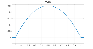
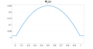
Figure 1: Comparison between mobility term $M_{0}(\phi)$ presented in (10) (left) and mobility term $M_{\varepsilon}(\phi)$ presented in (13) with $\varepsilon=0.015$ (right).

Then, using definition (13) we consider the approximate version of (11):

$$\left\{\begin{array}[]{rcl}\phi_{t}-\nabla\cdot(M_{\varepsilon}(\phi)\nabla\mu)&=&0\,,\\ \vskip 6.0pt plus 2.0pt minus 2.0pt\cr-\Delta\phi+F^{\prime}(\phi)&=&\mu\,,\end{array}\right.$$ (14)

subject to the same boundary and initial conditions presented in (6) and with the same energy (3) considered in the original problem (5). An existence result for problem (14) is also presented in [12].

In particular, under reasonable assumptions for the initial data $\phi_{0}$, the solution of problem (14) satisfy the following regularity results [12]:

• $\phi\in L^{\infty}(0,T;H^{1}(\Omega))\cap C([0,T];L^{2}(\Omega))\,,$

• $\phi_{t}\in L^{2}(0,T;(H^{1}(\Omega))^{\prime})\,,$

• $\mu\in L^{2}(0,T;H^{1}(\Omega))\,.$

Moreover, the following approximate boundedness results are provided:

$$\operatorname*{ess\,sup}_{0\leq t\leq T}\int_{\Omega}(\phi)_{-}^{2}d\boldsymbol{x}\leq C\varepsilon^{\alpha}\quad\quad\mbox{ and }\quad\quad\operatorname*{ess\,sup}_{0\leq t\leq T}\int_{\Omega}(\phi-1)_{+}^{2}d\boldsymbol{x}\leq C\varepsilon^{\alpha}\,,$$

with $\alpha=1$ in the case of the potential and mobility terms considered in this work.

In fact, these results are the main tools to show the existence and boundedness of solution of the degenerated problem (11) via a limit process as $\varepsilon\to 0$ (see [12]).

In particular, for the approximated model (14), the following result holds:

Lemma 1.

Any solution of the problem (14) and (6), satisfies the conservation property

$$\int_{\Omega}\phi(t,\boldsymbol{x})d\boldsymbol{x}\,=\,\int_{\Omega}\phi(0,\boldsymbol{x})d\boldsymbol{x}\quad\forall\,t>0$$ (15)

and the following integral version of the energy law

$$E(\phi(t))+\int_{0}^{t}\int_{\Omega}M_{\varepsilon}(\phi)|\nabla\mu|^{2}d\boldsymbol{x}\,d\tau=E(\phi_{0})\quad\mbox{ a.e. }t>0\,.$$ (16)

In particular, (16) implies the following estimates

$$\int_{\Omega}|\nabla\phi|^{2}d\boldsymbol{x}\in L^{\infty}(0,+\infty)\quad\mbox{ and }\quad\int_{\Omega}M_{\varepsilon}(\phi)|\nabla\mu|^{2}d\boldsymbol{x}\in L^{1}(0,+\infty)\,.$$ (17)

Proof.

We obtain (15) by testing (14)₁ by $1$. Moreover, testing equation (14)₁ by $\mu$ and (14)₂ by $\phi_{t}$ and working as in [12] we arrive at (16). ∎

The next step is to introduce two functionals $G_{\varepsilon}(\phi)$ and $J_{\varepsilon}(\phi)$ (defined from $M_{\varepsilon}(\phi)$) such that they satisfy estimates that will be helpful to show the approximate boundedness of the solution. Moreover, discrete versions of these estimates will prove useful when deriving the numerical schemes, in order to be able to show approximate maximum principle properties.

2.2.1 Functional $G_{\varepsilon}(\phi)$

Following the ideas in [12], we define a new functional $G_{\varepsilon}(\phi)$ by using the truncated mobility $M_{\varepsilon}(\phi)$ for a fixed truncation parameter $\varepsilon>0$:

$$G^{\prime\prime}_{\varepsilon}(\phi)\,:=\,\frac{1}{M_{\varepsilon}(\phi)}\quad\forall\,\phi\in\mathbb{R}\,.$$ (18)

Remark 2.

Denoting

$$G(\phi)\,:=\,\phi\ln(\phi)+(1-\phi)\ln(1-\phi)+1\quad\forall\,\phi\in[0,1]\,,$$

with

$$G^{\prime}(\phi)\,=\,\ln\left(\frac{\phi}{1-\phi}\right)\quad\forall\,\phi\in(0,1),$$

and

$$G^{\prime\prime}(\phi)\,=\,\frac{1}{\phi(1-\phi)}=\frac{1}{M(\phi)}\quad\forall\,\phi\in(0,1)\,,$$

then the functionals $G^{\prime\prime}_{\varepsilon}(\phi)$ in (18), $G^{\prime}_{\varepsilon}(\phi)$ and $G_{\varepsilon}(\phi)$ can be written as

$$G^{\prime}_{\varepsilon}(\phi)\,:=\,\left\{\begin{array}[]{ll}\displaystyle G^{\prime}(\varepsilon)+G^{\prime\prime}(\varepsilon)(\phi-\varepsilon)&\mbox{ if }\phi<\varepsilon\,,\\ \vskip 6.0pt plus 2.0pt minus 2.0pt\cr\displaystyle G^{\prime}(\phi)&\mbox{ if }\varepsilon\leq\phi\leq 1-\varepsilon\,,\\ \vskip 6.0pt plus 2.0pt minus 2.0pt\cr\displaystyle G^{\prime}(1-\varepsilon)+G^{\prime\prime}(1-\varepsilon)(\phi-(1-\varepsilon))&\mbox{ if }1-\varepsilon<\phi\,,\end{array}\right.$$

and

$$G_{\varepsilon}(\phi)\,:=\,\left\{\begin{array}[]{ll}\displaystyle G(\varepsilon)+G^{\prime}(\varepsilon)(\phi-\varepsilon)+\frac{1}{2}G^{\prime\prime}(\varepsilon)(\phi-\varepsilon)^{2}&\mbox{ if }\phi<\varepsilon\,,\\ \vskip 6.0pt plus 2.0pt minus 2.0pt\cr G(\phi)&\mbox{ if }\varepsilon\leq\phi\leq 1-\varepsilon\,,\\ \vskip 6.0pt plus 2.0pt minus 2.0pt\cr\displaystyle G(1-\varepsilon)+G^{\prime}(1-\varepsilon)(\phi-(1-\varepsilon))+\frac{1}{2}G^{\prime\prime}(1-\varepsilon)(\phi-(1-\varepsilon))^{2}&\mbox{ if }1-\varepsilon<\phi\,,\end{array}\right.$$

Remark 3.

Functional $G_{\varepsilon}(\phi)\in C^{2}(\mathbb{R})$ with $G_{\varepsilon}(\phi)\geq 0$, $G_{\varepsilon}^{\prime}(\varepsilon)<0$ and $G_{\varepsilon}^{\prime}(1-\varepsilon)>0$, then $G_{\varepsilon}(\phi)$ satisfy [12]

$$G_{\varepsilon}(\phi)\geq\displaystyle\frac{1}{2\varepsilon(1-\varepsilon)}(\phi-\varepsilon)^{2}\geq\displaystyle\frac{1}{2\varepsilon(1-\varepsilon)}\phi^{2}\quad\quad\forall\,\phi\leq\varepsilon$$

and

$$G_{\varepsilon}(\phi)\geq\displaystyle\frac{1}{2\varepsilon(1-\varepsilon)}(\phi-(1-\varepsilon))^{2}\geq\displaystyle\frac{1}{2\varepsilon(1-\varepsilon)}(\phi-1)^{2}\quad\forall\,\phi\geq 1-\varepsilon\,.$$

Lemma 2.

Any solution of the problem (14) and (6) satisfies the following relation a.e. $t>0$:

$$\int_{\Omega}G_{\varepsilon}(\phi(t))\,d\boldsymbol{x}+\int_{0}^{t}\int_{\Omega}\left((\Delta\phi)^{2}+\frac{3}{\eta^{2}}\left(\phi-\frac{1}{2}\right)^{2}|\nabla\phi|^{2}\right)d\boldsymbol{x}\,d\tau=\int_{\Omega}G_{\varepsilon}(\phi_{0})\,d\boldsymbol{x}+\frac{1}{4\eta^{2}}\int_{0}^{t}\int_{\Omega}|\nabla\phi|^{2}d\boldsymbol{x}\,d\tau\,.$$ (19)

Moreover, using estimates in (17), we can deduce

$$\left\|\int_{\Omega}G_{\varepsilon}(\phi(t,\cdot))d\boldsymbol{x}\right\|_{L^{\infty}(0,T)}+\int_{0}^{T}\int_{\Omega}(\Delta\phi)^{2}d\boldsymbol{x}dt\leq C\,\frac{T}{\eta^{2}}\,,$$

where $C$ depends on the initial energy $E(\phi_{0})$ and $\int_{\Omega}G_{\varepsilon}(\phi_{0})\,d\boldsymbol{x}$.

Proof.

Testing equation (14)₁ by $G_{\varepsilon}^{\prime}(\phi)$ and using that $M_{\varepsilon}(\phi)=1/G_{\varepsilon}^{\prime\prime}(\phi)$, we obtain

$$0\,=\,\displaystyle\int_{\Omega}\phi_{t}G_{\varepsilon}^{\prime}(\phi)d\boldsymbol{x}+\int_{\Omega}\frac{1}{G_{\varepsilon}^{\prime\prime}(\phi)}\nabla\mu\cdot\nabla G_{\varepsilon}^{\prime}(\phi)d\boldsymbol{x}\,.$$

Moreover, using the expression of $\mu$ in (14)₂ and the splitting presented in (8) we get

$$\begin{array}[]{rcl}\displaystyle\int_{\Omega}\nabla\mu\cdot\nabla\phi\,d\boldsymbol{x}&=&\displaystyle\int_{\Omega}\nabla\left(-\Delta\phi+F^{\prime}(\phi)\right)\cdot\nabla\phi\,d\boldsymbol{x}\\ \vskip 6.0pt plus 2.0pt minus 2.0pt\cr&=&\displaystyle\int_{\Omega}(\Delta\phi)^{2}d\boldsymbol{x}+\int_{\Omega}F_{c}^{\prime\prime}(\phi)|\nabla\phi|^{2}\,d\boldsymbol{x}+\int_{\Omega}F_{e}^{\prime\prime}(\phi)|\nabla\phi|^{2}\,d\boldsymbol{x}\,.\end{array}$$

Integrating in time, taking into account the equality [12]

$$\int_{0}^{t}\int_{\Omega}\phi_{t}G_{\varepsilon}^{\prime}(\phi)d\boldsymbol{x}=\int_{\Omega}G_{\varepsilon}(\phi(t))\,d\boldsymbol{x}-\int_{\Omega}G_{\varepsilon}(\phi(0))\,d\boldsymbol{x}\quad\mbox{ a.e. }t>0\,$$

and using (9) we arrive at (19).

∎

2.2.2 Functional $J_{\varepsilon}(\phi)$

We define a new functional $J_{\varepsilon}(\phi)$ by using the truncated mobility $M_{\varepsilon}(\phi)$ such that:

$$J^{\prime\prime}_{\varepsilon}(\phi)\,:=\,\frac{1}{\sqrt{M_{\varepsilon}(\phi)}}\quad\forall\,\phi\in\mathbb{R}\,.$$ (20)

Remark 4.

Denoting

$$J(\phi)\,:=\,(-2\phi+1)\arcsin\big{(}{\sqrt{1-\phi}}\big{)}+\sqrt{(1-\phi)\phi}+2\arcsin({\sqrt{1/2}})\phi\quad\forall\,\phi\in[0,1]\,,$$

with

$$J^{\prime}(\phi)\,=\,-2(\arcsin({\sqrt{1-\phi}})-\arcsin({\sqrt{1/2}}))\quad\forall\,\phi\in[0,1]$$

and

$$J^{\prime\prime}(\phi)\,=\,\frac{1}{\sqrt{\phi(1-\phi)}}=\frac{1}{\sqrt{M(\phi)}}\quad\forall\,\phi\in(0,1)\,,$$

then the functionals $J^{\prime\prime}_{\varepsilon}(\phi)$ in (20), $J^{\prime}_{\varepsilon}(\phi)$ and $J_{\varepsilon}(\phi)$ can be written as

$$J^{\prime}_{\varepsilon}(\phi)\,:=\,\left\{\begin{array}[]{ll}\displaystyle J^{\prime}(\varepsilon)+J^{\prime\prime}(\varepsilon)(\phi-\varepsilon)&\mbox{ if }\phi<\varepsilon\,,\\ \vskip 6.0pt plus 2.0pt minus 2.0pt\cr J^{\prime}(\phi)&\mbox{ if }\varepsilon\leq\phi\leq 1-\varepsilon\,,\\ \vskip 6.0pt plus 2.0pt minus 2.0pt\cr J^{\prime}(1-\varepsilon)+J^{\prime\prime}(1-\varepsilon)(\phi-(1-\varepsilon))&\mbox{ if }1-\varepsilon<\phi\,.\end{array}\right.$$

and

$$J_{\varepsilon}(\phi)\,:=\,\left\{\begin{array}[]{ll}\displaystyle J(\varepsilon)+J^{\prime}(\varepsilon)(\phi-\varepsilon)+\frac{1}{2}J^{\prime\prime}(\varepsilon)(\phi-\varepsilon)^{2}&\mbox{ if }\phi<\varepsilon\,,\\ \vskip 6.0pt plus 2.0pt minus 2.0pt\cr\displaystyle J(\phi)&\mbox{ if }\varepsilon\leq\phi\leq 1-\varepsilon\,,\\ \vskip 6.0pt plus 2.0pt minus 2.0pt\cr\displaystyle J(1-\varepsilon)+J^{\prime}(1-\varepsilon)(\phi-(1-\varepsilon))+\frac{1}{2}J^{\prime\prime}(1-\varepsilon)(\phi-(1-\varepsilon))^{2}&\mbox{ if }1-\varepsilon<\phi\,.\end{array}\right.$$

Remark 5.

Functional $J_{\varepsilon}(\phi)\in C^{2}(\mathbb{R})$ with $J_{\varepsilon}(\phi)\geq 0$, $J_{\varepsilon}^{\prime}(\varepsilon)<0$ and $J_{\varepsilon}^{\prime}(1-\varepsilon)>0$, then $J_{\varepsilon}(\phi)$ satisfy [12]

$$J_{\varepsilon}(\phi)\geq\displaystyle\frac{1}{2\sqrt{\varepsilon(1-\varepsilon)}}(\phi-\varepsilon)^{2}\geq\displaystyle\frac{1}{2\sqrt{\varepsilon(1-\varepsilon)}}\phi^{2}\quad\quad\forall\,\phi\leq\varepsilon$$

and

$$J_{\varepsilon}(\phi)\geq\displaystyle\frac{1}{2\sqrt{\varepsilon(1-\varepsilon)}}(\phi-(1-\varepsilon))^{2}\geq\displaystyle\frac{1}{2\sqrt{\varepsilon(1-\varepsilon)}}(\phi-1)^{2}\quad\forall\,\phi\geq 1-\varepsilon\,.$$

Lemma 3.

Any solution of the problem (14) and (6) satisfies the following inequality a.e. $t>0$:

$$\int_{\Omega}J_{\varepsilon}(\phi(t))\,d\boldsymbol{x}\leq\int_{\Omega}J_{\varepsilon}(\phi_{0})\,d\boldsymbol{x}+\int_{0}^{t}\int_{\Omega}\left(M_{\varepsilon}(\phi)|\nabla\mu|^{2}+\int_{\Omega}|\nabla\phi|^{2}\right)d\boldsymbol{x}\,d\tau\,.$$ (21)

Moreover, using estimates in (17) we can deduce

$$\left(\int_{\Omega}J_{\varepsilon}(\phi(t))\,d\boldsymbol{x}\right)\leq C_{1}+C_{2}t\,,\quad\hbox{a.e. $t>0$,}$$

with $C_{1}$ and $C_{2}$ are independent of $\eta$ (and depend on the initial energy $E(\phi_{0})$ and $\int_{\Omega}J_{\varepsilon}(\phi_{0})\,d\boldsymbol{x}$). Therefore we can also deduce

$$\left\|\int_{\Omega}J_{\varepsilon}(\phi(t,\cdot))d\boldsymbol{x}\right\|_{L^{\infty}(0,T)}\leq\Big{(}C_{1}+C_{2}T\Big{)}\,.$$

Proof.

Testing (14)₁ by $J_{\varepsilon}^{\prime}(\phi)$ and using (20) we obtain

$$\int_{\Omega}J_{\varepsilon}^{\prime}(\phi)\phi_{t}\,d\boldsymbol{x}+\int_{\Omega}\sqrt{M_{\varepsilon}(\phi)}\nabla\mu\cdot\nabla\phi\,d\boldsymbol{x}=0\,.$$

Integrating in time, and using $ab\leq{a^{2}}/2+{b^{2}}/2$, we can deduce (21).

∎

3 Two fully discrete numerical schemes

The numerical schemes proposed in this section are designed as approximations of the corresponding weak formulation of the system (14). Hereafter $(\cdot,\cdot)$ denotes the $L^{2}(\Omega)$-scalar product. For all numerical schemes we consider a partition of the time interval $[0,T]$ into $N$ subintervals, with constant time step $\Delta t=T/N$ and we denote by $\delta_{t}$ the (backward) discrete time derivative

$$\delta_{t}f\,:=\,\frac{f^{n+1}-f^{n}}{\Delta t}\,.$$

We consider structured triangulations $\{\mathcal{T}_{h}\}$ of the domain $\Omega$ with its elements denoted by $I_{i}$, that is $\{\mathcal{T}_{h}\}=\bigcup_{i}I_{i}$ with the size of elements being bounded by $h>0$. The unknowns $(\phi,\mu)$ are approximated by the $C^{0}$-Finite Elements spaces of order $k\geq 1$ (denoted by $\mathbb{P}_{k}$):

$$(\phi,\mu)\in\Phi_{h}\times W_{h}=\mathbb{P}_{1}\times\mathbb{P}_{k}\,.$$

Moreover, we need to use mass-lumping ideas [6] to help us achieve boundedness of the unknown $\phi$. To this end we introduce the discrete semi-inner product on $C^{0}(\overline{\Omega})$ and its induced discrete semi-norm:

$$(f,g)_{h}\,:=\,\int_{\Omega}I_{h}(fg)d\boldsymbol{x}\quad\mbox{ and }\quad|f|_{h}\,:=\,\sqrt{(f,f)_{h}}\,,$$

with $I_{h}(f(\boldsymbol{x}))$ denoting the nodal $\mathbb{P}_{1}$-interpolation of the function $f(\boldsymbol{x})$. We use $f_{+}$ or $f_{-}$ to denote the positive or negative part of a function $f$ ($f_{+}(\boldsymbol{x})=\max\{f(\boldsymbol{x}),0\}$ and $f_{-}(\boldsymbol{x})=\min\{f(\boldsymbol{x}),0\}$).

We propose two numerical schemes, called G_ε-scheme and J_ε-scheme, designed to take advantage of the discrete versions of the estimates for $G_{\varepsilon}(\phi)$ (19) and $J_{\varepsilon}(\phi)$ (21), respectively. Both schemes will be conservative and energy stable, that is, they will maintain the amount of phase constant in time ($\int_{\Omega}\phi^{n+1}=\int_{\Omega}\phi^{n}$) and they will satisfy discrete versions of the energy law (16), which in particular imply the energy decreasing property ($E(\phi^{n+1})\leq E(\phi^{n})$). In fact, the key point to achieve the energy stability of the schemes is to take advantage of the splitting in (8) and to consider the ideas of Eyre [13], i.e., take implicitly the convex part and explicitly the concave part because the following relation holds:

$$\frac{1}{\Delta t}\int_{\Omega}\Big{(}F^{\prime}_{c}(\phi^{n+1})+F^{\prime}_{e}(\phi^{n})\Big{)}(\phi^{n+1}-\phi^{n})d\boldsymbol{x}\,\geq\,\frac{1}{\Delta t}\int_{\Omega}\Big{(}F(\phi^{n+1})-F(\phi^{n})\Big{)}d\boldsymbol{x}\,.$$ (22)

3.1 G_ε-scheme

The G_ε-scheme is defined as follows: Given $\phi^{n}\in\Phi_{h}$, find $(\phi^{n+1},\mu^{n+1})\in\Phi_{h}\times M_{h}$ such that

$$\left\{\begin{array}[]{rcl}\displaystyle\frac{1}{\Delta t}\big{(}\phi^{n+1}-\phi^{n},\bar{\mu}\big{)}_{h}+\big{(}M^{G}_{\varepsilon}(\phi^{n+1})\nabla\mu^{n+1},\nabla\bar{\mu}\big{)}&=&0\,,\\ \vskip 6.0pt plus 2.0pt minus 2.0pt\cr(\nabla\phi^{n+1},\nabla\bar{\phi})+\big{(}I_{h}(F_{c}^{\prime}(\phi^{n+1}))+I_{h}(F_{e}^{\prime}(\phi^{n})),\bar{\phi}\big{)}_{h}&=&(\mu^{n+1},\bar{\phi})_{h}\,,\end{array}\right.$$ (23)

for all $(\bar{\phi},\bar{\mu})\in\Phi_{h}\times M_{h}$, where $M^{G}_{\varepsilon}(\phi)$ for any $\phi\in\Phi_{h}=\mathbb{P}_{1}$ will be an adequate $\mathbb{P}_{0}$ approximation of $M_{\varepsilon}(\phi)=1/G^{\prime\prime}_{\varepsilon}(\phi)$ (owing to (18)), satisfying the $\mathbb{P}_{0}$ discrete equality

$$M^{G}_{\varepsilon}(\phi)\,\nabla I_{h}\Big{(}G^{\prime}_{\varepsilon}(\phi)\Big{)}=\nabla\phi\quad\forall\,\phi\in\Phi_{h}\,.$$ (24)

Indeed, $M^{G}_{\varepsilon}(\phi)$ for any $\phi\in\Phi_{h}$ will be a diagonal matrix function, denoting its diagonal elements $M^{G}_{kk}$ for $k=1,\dots,d$. For each element $I_{i}$ of the triangulation $\{\mathcal{T}_{h}\}$ (with nodes $\boldsymbol{x}_{0}$, $\boldsymbol{x}_{k}$ in the $k$-th axis) we compute the $\mathbb{P}_{0}$ function

$$M^{G}_{kk}\Big{|}_{I_{i}}\,:=\,\left\{\begin{array}[]{cc}\displaystyle\frac{\phi(\boldsymbol{x}_{k})-\phi(\boldsymbol{x}_{0})}{G^{\prime}_{\varepsilon}(\phi(\boldsymbol{x}_{k}))-G^{\prime}_{\varepsilon}(\phi(\boldsymbol{x}_{0}))}&\mbox{ if }\phi(\boldsymbol{x}_{0})\neq\phi(\boldsymbol{x}_{k})\,,\\ \vskip 6.0pt plus 2.0pt minus 2.0pt\cr\displaystyle\frac{1}{G^{\prime\prime}_{\varepsilon}(\phi(\boldsymbol{x}_{0}))}&\mbox{ if }\phi(\boldsymbol{x}_{0})=\phi(\boldsymbol{x}_{k})\,.\end{array}\right.$$ (25)

In fact, since $\Phi_{h}=\mathbb{P}_{1}$, the relation (24) holds as a $\mathbb{P}_{0}$ equality. Note that $M^{G}_{kk}\Big{|}_{I_{i}}\geq 0$ owing to the convexity of $G_{\varepsilon}(\phi)$.

Remark 6.

$M^{G}_{\varepsilon}(\phi)$ can be understood as a non-centered modification of the mobility $M_{\varepsilon}(\phi)$ in such a way that both practically coincide when $\phi$ is located around the center $\phi=1/2$ of the interval $(0,1)$ but they differ when the values of $\phi$ are close to $0$ and $1$ (see Figure 2). We observe how this non-centered mobility $M^{G}_{\varepsilon}(\phi)$ is going to zero at the endpoints $\phi=0$ and $\phi=1$ faster than $M_{\varepsilon}(\phi)$, as $\varepsilon$ goes to zero, which will help to control the boundedness of the unknown $\phi$ between $0$ and $1$ in the numerical scheme.

Figure 2: Comparison of $M_{\varepsilon}(\phi)$ with $M^{G}_{\varepsilon}(\phi)$ (left) and $M^{J}_{\varepsilon}(\phi)$ (right) by plotting their difference in the interval $\phi\in[0.01,0.99]$.

Remark 7.

In order to be able to construct the matrix $M^{G}_{\varepsilon}(\phi)$ we need to use the requirement of considering structured triangulations of $\Omega$.

3.1.1 Conservation of volume and energy-stability

Lemma 4.

Any solution $(\phi^{n+1},\mu^{n+1})\in\Phi_{h}\times M_{h}$ of the G_ε-scheme (23) satisfies the conservation property

$$\int_{\Omega}\phi^{n+1}d\boldsymbol{x}\,=\,\int_{\Omega}\phi^{n}d\boldsymbol{x}$$ (26)

and the following discrete version of the energy law (16):

$$\delta_{t}E_{h}(\phi^{n+1})+\displaystyle\int_{\Omega}\left|\sqrt{M^{G}_{\varepsilon}(\phi^{n+1})}\nabla\mu^{n+1}\right|^{2}d\boldsymbol{x}\leq 0\,,$$ (27)

where

$$E_{h}(\phi)=\int_{\Omega}\frac{1}{2}|\nabla\phi|^{2}+\int_{\Omega}I_{h}(F(\phi))\,.$$

Proof.

We obtain (26) by taking $\bar{\mu}=1$ in (23)₁. Moreover, by testing equation (23)₂ by $\bar{\phi}=\frac{1}{\Delta t}(\phi^{n+1}-\phi^{n})$, equation (23)₁ by $\bar{\mu}=\mu^{n+1}$ and using (22) we arrive at (27). ∎

3.1.2 Approximated maximum principle

Lemma 5.

If $M_{h}=\mathbb{P}_{1}$ (hence $\Phi_{h}=M_{h}$), then any solution $(\phi^{n+1},\mu^{n+1})\in\Phi_{h}\times M_{h}$ of the G_ε-scheme (23) satisfies the following discrete version of (19):

$$\begin{array}[]{c}\displaystyle\delta_{t}\left(\int_{\Omega}I_{h}(G_{\varepsilon}(\phi^{n+1}))d\boldsymbol{x}\right)+\displaystyle\int_{\Omega}I_{h}\Big{(}(\omega^{n+1})^{2}\Big{)}d\boldsymbol{x}+\int_{\Omega}\left|\sqrt{R(\phi^{n+1})}\nabla\phi^{n+1}\right|^{2}d\boldsymbol{x}\\ \vskip 6.0pt plus 2.0pt minus 2.0pt\cr\leq\displaystyle\frac{1}{8\eta^{2}}\left(\int_{\Omega}|\nabla\phi^{n}|^{2}d\boldsymbol{x}+\int_{\Omega}|\nabla\phi^{n+1}|^{2}d\boldsymbol{x}\right)\,,\end{array}$$ (28)

with $\omega^{n+1}=\mu^{n+1}-\big{(}I_{h}(F_{c}^{\prime}(\phi^{n+1}))+I_{h}(F_{e}^{\prime}(\phi^{n}))\big{)}$ and $R(\phi)$ being a positive semidefinite diagonal matrix function (related to $F^{\prime\prime}_{c}(\phi))$, defined by

$$R_{kk}\Big{|}_{I_{i}}\,:=\,\left\{\begin{array}[]{cc}\displaystyle\frac{F^{\prime}_{c}(\phi(\boldsymbol{x}_{k}))-F^{\prime}_{c}(\phi(\boldsymbol{x}_{0}))}{\phi(\boldsymbol{x}_{k})-\phi(\boldsymbol{x}_{0})}&\mbox{ if }\phi(\boldsymbol{x}_{0})\neq\phi(\boldsymbol{x}_{k})\,,\\ \vskip 6.0pt plus 2.0pt minus 2.0pt\cr\displaystyle{F^{\prime\prime}_{c}(\phi(\boldsymbol{x}_{0}))}&\mbox{ if }\phi(\boldsymbol{x}_{0})=\phi(\boldsymbol{x}_{k})\,.\end{array}\right.$$

Note that $R_{kk}\Big{|}_{I_{i}}\geq 0$ owing to the convexity of $F_{c}(\phi)$.

Moreover, using (27) we can deduce

$$\int_{\Omega}I_{h}(G_{\varepsilon}(\phi^{n+1}))d\boldsymbol{x}\leq C\,\frac{T}{\eta^{2}}\,,$$ (29)

where $C$ depends on the initial energy $E(\phi^{0})$ and $\int_{\Omega}I_{h}(G_{\varepsilon}(\phi^{0}))d\boldsymbol{x}$.

Proof.

Testing equation (23)₁ by $\bar{\mu}=I_{h}(G^{\prime}(\phi^{n+1}))$ and using property (24) we get:

$$\int_{\Omega}I_{h}\Big{(}\delta_{t}\phi^{n+1}\,G_{\varepsilon}^{\prime}(\phi^{n+1})\Big{)}d\boldsymbol{x}\,+\,(\nabla\mu^{n+1},\nabla\phi^{n+1})\,=\,0\,.$$

By introducing the auxiliary variable $\omega^{n+1}=\mu^{n+1}-\big{(}I_{h}(F_{c}^{\prime}(\phi^{n+1}))+I_{h}(F_{e}^{\prime}(\phi^{n}))\big{)}\in\mathbb{P}_{1}$ (because $M_{h}=\mathbb{P}_{1}$) we can rewrite (23)₂ as

$$(\omega^{n+1},\bar{\phi})_{h}=(\nabla\phi^{n+1},\nabla\bar{\phi})\quad\forall\,\bar{\phi}\in\Phi_{h}\,,$$

therefore taking first $\bar{\phi}=\mu^{n+1}\in\mathbb{P}_{1}$ and afterwards $\bar{\phi}=I_{h}(F_{c}^{\prime}(\phi^{n+1}))+I_{h}(F_{e}^{\prime}(\phi^{n}))\in\mathbb{P}_{1}$, one has

$$\begin{array}[]{rcl}\displaystyle(\nabla\mu^{n+1},\nabla\phi^{n+1})&=&\displaystyle(\omega^{n+1},\mu^{n+1})_{h}\\ \vskip 6.0pt plus 2.0pt minus 2.0pt\cr&=&\displaystyle\Big{(}\omega^{n+1},\omega^{n+1}+I_{h}(F_{c}^{\prime}(\phi^{n+1}))+I_{h}(F_{e}^{\prime}(\phi^{n}))\Big{)}_{h}\\ \vskip 6.0pt plus 2.0pt minus 2.0pt\cr&=&\displaystyle\int_{\Omega}I_{h}\Big{(}(\omega^{n+1})^{2}\Big{)}d\boldsymbol{x}+\int_{\Omega}\nabla\phi^{n+1}\cdot\nabla\big{(}I_{h}(F_{c}^{\prime}(\phi^{n+1}))+I_{h}(F_{e}^{\prime}(\phi^{n}))\big{)}d\boldsymbol{x}\,,\end{array}$$

hence

$$\int_{\Omega}I_{h}\Big{(}\delta_{t}\phi^{n+1}\,G_{\varepsilon}^{\prime}(\phi^{n+1})\Big{)}+I_{h}\Big{(}(\omega^{n+1})^{2}\Big{)}+\nabla\Big{(}I_{h}(F_{c}^{\prime}(\phi^{n+1}))+I_{h}(F_{e}^{\prime}(\phi^{n}))\Big{)}\cdot\nabla\phi^{n+1}=0\,.$$ (30)

By using Taylor expansion and the convexity of $G_{\varepsilon}(\phi)$ ($G_{\varepsilon}^{\prime\prime}(\phi)\geq 0$), we obtain

$$\int_{\Omega}I_{h}\Big{(}\delta_{t}\phi^{n+1}\,G_{\varepsilon}^{\prime}(\phi^{n+1})\Big{)}d\boldsymbol{x}\geq\delta_{t}\int_{\Omega}I_{h}(G_{\varepsilon}(\phi^{n+1}))d\boldsymbol{x}\,.$$ (31)

Because $F^{\prime}_{e}$ is linear $(I_{h}(F^{\prime}_{e}(\phi))=F^{\prime}_{e}(\phi))$ we can deduce that

$$-\displaystyle\int_{\Omega}\nabla I_{h}(F_{e}^{\prime}(\phi^{n}))\cdot\nabla\phi^{n+1}d\boldsymbol{x}=\frac{1}{4\eta^{2}}\displaystyle\int_{\Omega}\nabla\phi^{n}\cdot\nabla\phi^{n+1}d\boldsymbol{x}\leq\frac{1}{8\eta^{2}}\left(\int_{\Omega}|\nabla\phi^{n}|^{2}d\boldsymbol{x}+\int_{\Omega}|\nabla\phi^{n+1}|^{2}d\boldsymbol{x}\right)\,.$$ (32)

Now, taking into account that the mesh is structured and $F^{\prime\prime}_{c}(\phi)\geq 0$ for all $\phi\in\mathbb{R}$, we consider the $\mathbb{P}_{0}$ positive semidefinite diagonal matrix function $R(\phi^{n+1})$ which satisfies

$$\nabla I_{h}(F_{c}^{\prime}(\phi^{n+1}))=R(\phi^{n+1})\nabla\phi^{n+1}\,,$$

which implies

$$\nabla I_{h}(F_{c}^{\prime}(\phi^{n+1}))\cdot\nabla\phi^{n+1}=\Big{(}R(\phi^{n+1})\nabla\phi^{n+1}\Big{)}\cdot\nabla\phi^{n+1}=\left|\sqrt{R(\phi^{n+1})}\nabla\phi^{n+1}\right|^{2}.$$ (33)

Therefore, using (31), (32) and (33) in (30) we obtain (28). ∎

Corollary 1.

If $\Phi_{h}=M_{h}=\mathbb{P}_{1}$, any solution $(\phi^{n+1},\mu^{n+1})\in\Phi_{h}\times M_{h}$ of G_ε-scheme (23) satisfies the following estimates:

$$\int_{\Omega}\big{(}I_{h}(\phi_{-}^{n+1})\big{)}^{2}d\boldsymbol{x}\leq C\,\frac{\varepsilon(1-\varepsilon)}{\eta^{2}}\leq C\,\frac{\varepsilon}{\eta^{2}}$$ (34)

and

$$\int_{\Omega}\Big{(}I_{h}\big{(}(\phi^{n+1}-1)_{+}\big{)}\Big{)}^{2}d\boldsymbol{x}\leq C\,\frac{\varepsilon(1-\varepsilon)}{\eta^{2}}\leq C\,\frac{\varepsilon}{\eta^{2}}\,,$$ (35)

where $C$ depends on the initial energy $E(\phi^{0})$ and $\int_{\Omega}I_{h}(G_{\varepsilon}(\phi^{0}))d\boldsymbol{x}$.

Proof.

The main ideas of this proof were already used in [14]. From Remark 3 and taking into account that $G_{\varepsilon}(\phi)\geq 0$ for all $\phi\in\mathbb{R}$ we have

$$G_{\varepsilon}(\phi)\geq\displaystyle\frac{1}{2\varepsilon(1-\varepsilon)}(\phi_{-})^{2}\quad\mbox{ and }\quad G_{\varepsilon}(\phi)\geq\displaystyle\frac{1}{2\varepsilon(1-\varepsilon)}\big{(}(\phi-1)_{+}\big{)}^{2}\quad\forall\,\phi\in\mathbb{R}\,.$$

Then, using that

$$\big{(}I_{h}(\phi)\big{)}^{2}\leq I_{h}(\phi^{2})\quad\forall\,\phi\in C^{0}(\overline{\Omega})\,,$$

we obtain

$$\int_{\Omega}I_{h}\big{(}G_{\varepsilon}(\phi^{n+1})\big{)}d\boldsymbol{x}\geq\displaystyle\frac{1}{2\varepsilon(1-\varepsilon)}\int_{\Omega}I_{h}\big{(}(\phi^{n+1}_{-})^{2}\big{)}d\boldsymbol{x}\geq\displaystyle\frac{1}{2\varepsilon(1-\varepsilon)}\int_{\Omega}\big{(}I_{h}(\phi^{n+1}_{-})\big{)}^{2}d\boldsymbol{x}\,$$

and

$$\int_{\Omega}I_{h}\big{(}G_{\varepsilon}(\phi^{n+1})\big{)}d\boldsymbol{x}\geq\displaystyle\frac{1}{2\varepsilon(1-\varepsilon)}\int_{\Omega}I_{h}\Big{(}\big{(}(\phi^{n+1}-1)_{+}\big{)}^{2}\Big{)}d\boldsymbol{x}\geq\displaystyle\frac{1}{2\varepsilon(1-\varepsilon)}\int_{\Omega}\Big{(}I_{h}\big{(}(\phi^{n+1}-1)_{+}\big{)}\Big{)}^{2}d\boldsymbol{x}\,.$$

Finally, combining previous expressions with estimate (29) we obtain (34) and (35). ∎

Remark 8.

G_ε-scheme (23) satisfies an approximate maximum principle for $\phi^{n+1}$, because estimates (34) and (35) imply in particular that

$$I_{h}(\phi^{n+1}_{-})\rightarrow 0\quad\mbox{ and }\quad I_{h}\big{(}(\phi^{n+1}-1)_{+}\big{)}\rightarrow 0\quad\mbox{ in }L^{2}(\Omega),\quad\mbox{ as }\quad\varepsilon\rightarrow 0\,,$$

with $\mathcal{O}\left(\sqrt{\varepsilon}/\eta\right)$ accuracy rate.

3.2 J_ε-scheme

The J_ε-scheme is defined as follows: Given $\phi^{n}\in\Phi_{h}=\mathbb{P}_{1}$, find $(\phi^{n+1},\mu^{n+1})\in\Phi_{h}\times M_{h}$ such that:

$$\left\{\begin{array}[]{rcl}\displaystyle\frac{1}{\Delta t}(\phi^{n+1}-\phi^{n},\bar{\mu})_{h}+(M^{J}_{\varepsilon}(\phi^{n+1})\nabla\mu^{n+1},\nabla\bar{\mu})&=&0\,,\\ \vskip 6.0pt plus 2.0pt minus 2.0pt\cr(\nabla\phi^{n+1},\nabla\bar{\phi})+\big{(}F^{\prime}_{c}(\phi^{n+1})+F^{\prime}_{e}(\phi^{n}),\bar{\phi}\big{)}&=&(\mu^{n+1},\bar{\phi})_{h}\,,\end{array}\right.$$ (36)

for all $(\bar{\phi},\bar{\mu})\in\Phi_{h}\times M_{h}$ with $M^{J}_{\varepsilon}(\phi^{n+1})$ being an approximation of $\left(1/J^{\prime\prime}_{\varepsilon}(\phi^{n+1})\right)^{2}$. In particular, for any $\phi\in\Phi_{h}=\mathbb{P}_{1}$, $M^{J}_{\varepsilon}(\phi)$ is a diagonal matrix with elements $M^{J}_{kk}$ for $k=1,\dots,d$. That is, for each element $I_{i}$ of the triangulation $\{\mathcal{T}_{h}\}$ (with nodes $\boldsymbol{x}_{0}$, $\boldsymbol{x}_{k}$ in the $k$-th axis) we compute the $\mathbb{P}_{0}$ function

$$M^{J}_{kk}\Big{|}_{I_{i}}\,:=\,\left\{\begin{array}[]{cc}\displaystyle\left(\frac{\phi(\boldsymbol{x}_{k})-\phi(\boldsymbol{x}_{0})}{J^{\prime}_{\varepsilon}(\phi(\boldsymbol{x}_{k}))-J^{\prime}_{\varepsilon}(\phi(\boldsymbol{x}_{0}))}\right)^{2}&\mbox{ if }\phi(\boldsymbol{x}_{0})\neq\phi(\boldsymbol{x}_{k})\,,\\ \vskip 6.0pt plus 2.0pt minus 2.0pt\cr\displaystyle\left(\frac{1}{J^{\prime\prime}_{\varepsilon}(\phi(\boldsymbol{x}_{0}))}\right)^{2}&\mbox{ if }\phi(\boldsymbol{x}_{0})=\phi(\boldsymbol{x}_{k})\,.\end{array}\right.$$ (37)

In fact, using that $\Phi_{h}=\mathbb{P}_{1}$, the following $\mathbb{P}_{0}$ relation holds:

$$M^{J}_{\varepsilon}(\phi)\,\nabla I_{h}\Big{(}J^{\prime}_{\varepsilon}(\phi)\Big{)}=\sqrt{M^{J}_{\varepsilon}(\phi)}\nabla\phi\,,\quad\forall\,\phi\in\Phi_{h}\,.$$ (38)

Remark 9.

$M^{J}_{\varepsilon}(\phi)$ can be understood as a non-centered modification of the mobility $M_{\varepsilon}(\phi)$ in such a way that both practically coincide when $\phi$ is located around the center $\phi=1/2$ of the interval $(0,1)$ but they differ when the values of $\phi$ are close to $0$ and $1$ (see Figure 2). We observe how this non-centered mobility $M^{J}_{\varepsilon}(\phi)$ is going to zero at the endpoints $\phi=0$ and $\phi=1$ faster than $M_{\varepsilon}(\phi)$, as $\varepsilon$ goes to zero, which will help to control the boundedness of the unknown $\phi$ between $0$ and $1$ in the numerical scheme.

Remark 10.

In order to be able to construct the matrix $M^{J}_{\varepsilon}(\phi)$ we need to use the requirement of considering structured triangulations of $\Omega$.

3.2.1 Conservation of volume and energy-stability

Lemma 6.

Any solution of the $J_{\varepsilon}$-scheme (36) satisfies the conservation property

$$\int_{\Omega}\phi^{n+1}d\boldsymbol{x}\,=\,\int_{\Omega}\phi^{n}d\boldsymbol{x}$$ (39)

and the following discrete version of the energy law (16):

$$\delta_{t}E(\phi^{n+1})\,+\,\displaystyle\int_{\Omega}M^{J}_{\varepsilon}(\phi^{n+1})|\nabla\mu^{n+1}|^{2}d\boldsymbol{x}\,\leq\,0\,,$$ (40)

where $E(\phi)$ is defined in (3).

Proof.

We obtain (39) by taking $\bar{\mu}=1$ in (36)₁. Moreover, testing equation (36)₁ by $\bar{\mu}=\mu^{n+1}$, equation (36)₂ by $\bar{\phi}=\frac{1}{\Delta t}(\phi^{n+1}-\phi^{n})$ and using (22) we arrive at (40). ∎

3.2.2 Approximated maximum principle

Lemma 7.

If $M_{h}=\mathbb{P}_{1}$ (hence $\Phi_{h}=M_{h}$), then any solution of the $J_{\varepsilon}$-scheme (36) satisfies the following discrete version of estimate (21):

$$\delta_{t}\left(\int_{\Omega}I_{h}(J_{\varepsilon}(\phi^{n+1}))\right)\,\leq\,\int_{\Omega}M^{J}_{\varepsilon}(\phi^{n+1})|\nabla\mu^{n+1}|^{2}d\boldsymbol{x}+\displaystyle\int_{\Omega}|\nabla\phi^{n+1}|^{2}d\boldsymbol{x}\,.$$ (41)

Moreover, using (40) we can deduce

$$\int_{\Omega}I_{h}(J_{\varepsilon}(\phi^{n+1}))d\boldsymbol{x}\leq C_{1}+C_{2}\,T\,,$$ (42)

where $C_{1}$ and $C_{2}$ depend on the initial energy $E(\phi^{0})$ and of $\int_{\Omega}I_{h}(J_{\varepsilon}(\phi^{0}))$.

Proof.

Testing equation (36)₁ by $\bar{\mu}=I_{h}(J^{\prime}(\phi^{n+1}))$ and using relation (38) we obtain:

$$\begin{array}[]{rcl}\displaystyle\int_{\Omega}I_{h}\Big{(}\delta_{t}\phi^{n+1}\,J^{\prime}(\phi^{n+1})\Big{)}d\boldsymbol{x}&=&\displaystyle-\int_{\Omega}\sqrt{M^{J}_{\varepsilon}(\phi^{n+1})}\nabla\mu^{n+1}\cdot\nabla\phi^{n+1}d\boldsymbol{x}\\ \vskip 6.0pt plus 2.0pt minus 2.0pt\cr&\leq&\displaystyle\int_{\Omega}\left|\sqrt{M^{J}_{\varepsilon}(\phi^{n+1})}\nabla\mu^{n+1}\right|^{2}d\boldsymbol{x}+\displaystyle\int_{\Omega}|\nabla\phi^{n+1}|^{2}d\boldsymbol{x}\,.\end{array}$$

By using Taylor expansion and the convexity of $J_{\varepsilon}(\phi)$ (as for $G_{\varepsilon}(\phi)$ in (31)), we deduce (41). ∎

Corollary 2.

Any solution $(\phi^{n+1},\mu^{n+1})$ of J_ε-scheme (36) satisfies the following estimates:

$$\int_{\Omega}\big{(}I_{h}(\phi_{-}^{n+1})\big{)}^{2}d\boldsymbol{x}\leq C\,\sqrt{\varepsilon(1-\varepsilon)}\leq C\,\sqrt{\varepsilon}$$ (43)

and

$$\int_{\Omega}\Big{(}I_{h}\big{(}(\phi^{n}-1)_{+}\big{)}\Big{)}^{2}d\boldsymbol{x}\leq C\,\sqrt{\varepsilon(1-\varepsilon)}\leq C\,\sqrt{\varepsilon}\,,$$ (44)

where $C$ depends on the initial energy $E(\phi^{0})$ and $\int_{\Omega}I_{h}(J_{\varepsilon}(\phi^{0}))$.

Proof.

Following the same steps presented in Lemma 1, but now using Remark 5 and estimate (42). ∎

Remark 11.

J_ε-scheme (36) satisfies an approximate minimum principle for $\phi^{n+1}$, because estimates (43) and (44) imply in particular that

$$I_{h}(\phi^{n+1}_{-})\rightarrow 0\quad\mbox{ and }\quad I_{h}\big{(}(\phi^{n+1}-1)_{+}\big{)}\rightarrow 0\quad\mbox{ in }L^{2}(\Omega)\quad\mbox{ as }\quad\varepsilon\rightarrow 0\,,$$

with $\mathcal{O}\left(\sqrt[4]{\varepsilon}\right)$ accuracy rate.

4 Numerical simulations

The implementation of the numerical schemes follows the same ideas in any spatial dimension, but for the sake of simplicity to illustrate the properties of the schemes, most of the numerical experiments reported in this section have been carried out in a one dimensional domain $\Omega=(0,1)$ using MATLAB [25]. At the end of the section we present one numerical experiment in a $2D$-domain using Freefem++ [19] to evidence that the proposed ideas also work in higher dimensions. In fact, although the implementation of $M^{G}_{\varepsilon}(\phi)$ and $M^{J}_{\varepsilon}(\phi)$ might seem rather complicated due to the need of comparing values of the unknown $\phi$ in different nodes of the each element of the triangulation, it can be easily done by checking the values of the corresponding $\mathbb{P}_{0}$ functions that form $\nabla\phi$.

Moreover, we remind the reader that parameter $\eta$ is associated with the width of the interface, so the size of the spatial mesh should always be small enough to capture the interface, hence one must consider at least $h\leq\eta$. On the other hand, parameter $\varepsilon$ determine the separation of the mobility from zero, which does not have any relation with the spatial mesh size. In fact, due to the advancement on computing resources, we can take very small values of the parameter $\varepsilon$ (the lowest in this work is $\varepsilon=10^{-20}$) without being close to the machine precision of the computer.

4.1 M₀-scheme

In order to better comprehend the properties of the proposed schemes, we have compared them with the corresponding FE scheme with the truncated by zero mobility $M_{0}(\phi)$, which has been approximated implicitly in time. The scheme reads: Find $(\phi^{n+1},\mu^{n+1})\in\Phi_{h}\times M_{h}$ solving

$$\left\{\begin{array}[]{rcl}\displaystyle\frac{1}{\Delta t}(\phi^{n+1}-\phi^{n},\bar{\mu})+(M_{0}(\phi^{n+1})\nabla\mu^{n+1},\nabla\bar{\mu})&=&0\,,\\ \vskip 6.0pt plus 2.0pt minus 2.0pt\cr(\nabla\phi^{n+1},\nabla\bar{\phi})+\big{(}F^{\prime}_{c}(\phi^{n+1})+F^{\prime}_{e}(\phi^{n}),\bar{\phi}\big{)}&=&(\mu^{n+1},\bar{\phi})\,,\end{array}\right.$$ (45)

for all $(\bar{\phi},\bar{\mu})\in\Phi_{h}\times M_{h}$. This type of FE scheme is the standard by default used in this problem, in order to be sure that even if $\phi$ goes outside of the interval $[0,1]$ the mobility $M_{0}(\phi)$ will never become negative. Moreover, this scheme is energy stable since the following result holds.

Lemma 8.

Any solution of the M₀-scheme (45) satisfies the following discrete version of the energy law (16):

$$\delta_{t}E(\phi^{n+1})\,+\,\displaystyle\int_{\Omega}M_{0}(\phi^{n+1})|\nabla\mu^{n+1}|^{2}d\boldsymbol{x}\,\leq\,0\,.$$

Proof.

Testing equation (45)₁ by $\bar{\mu}=\mu^{n+1}$, equation (45)₂ by $\bar{\phi}=\frac{1}{\Delta t}(\phi^{n+1}-\phi^{n})$ and using (22). ∎

Remark 12.

No results about the boundedness of $\phi^{n}$ in $[0,1]$ are known for M₀-scheme (45).

4.2 Picard iterative algorithms

Now we describe the iterative algorithms considered to approximate the nonlinear G_ε-scheme (23), J_ε-scheme (36) and M₀-scheme (45). Let $(\phi^{n},\mu^{n})$ and $(\phi^{\ell},\mu^{\ell})$ be known (we consider initially $(\phi^{\ell=0},\mu^{\ell=0})=(\phi^{n},\mu^{n})$), compute $(\phi^{\ell+1},\mu^{\ell+1})$ such that:

4.2.1 Iterative algorithm for G_ε-scheme

$$\left\{\begin{array}[]{rcl}\displaystyle\frac{1}{\Delta t}(\phi^{\ell+1},\bar{\mu})_{h}+\Big{(}M^{G}_{\varepsilon}(\phi^{l})\nabla\mu^{l+1},\nabla\bar{\mu}\Big{)}&=&\displaystyle\frac{1}{\Delta t}(\phi^{n},\bar{\mu})_{h}\,,\\ \vskip 6.0pt plus 2.0pt minus 2.0pt\cr(\mu^{\ell+1},\bar{\phi})_{h}-(\nabla\phi^{\ell+1},\nabla\bar{\phi})&=&\Big{(}I_{h}(F_{c}^{\prime}(\phi^{l}))+I_{h}(F_{e}^{\prime}(\phi^{n})),\bar{\phi}\Big{)}_{h}\,.\end{array}\right.$$

4.2.2 Iterative algorithm for J_ε-scheme

$$\left\{\begin{array}[]{rcl}\displaystyle\frac{1}{\Delta t}(\phi^{\ell+1},\bar{\mu})_{h}+(M^{J}_{\varepsilon}(\phi^{\ell})\nabla\mu^{\ell+1},\nabla\bar{\mu})&=&\displaystyle\frac{1}{\Delta t}(\phi^{n},\bar{\mu})_{h}\,,\\ \vskip 6.0pt plus 2.0pt minus 2.0pt\cr(\mu^{n+1},\bar{\phi})_{h}-(\nabla\phi^{\ell+1},\nabla\bar{\phi})&=&(F^{\prime}_{c}(\phi^{\ell})+F^{\prime}_{e}(\phi^{n}),\bar{\phi})\,.\end{array}\right.$$

4.2.3 Iterative algorithm for M₀-scheme

$$\left\{\begin{array}[]{rcl}\displaystyle\frac{1}{\Delta t}(\phi^{\ell+1},\bar{\mu})+(M_{0}(\phi^{\ell})\nabla\mu^{\ell+1},\nabla\bar{\mu})&=&\displaystyle\frac{1}{\Delta t}(\phi^{n},\bar{\mu})\,,\\ \vskip 6.0pt plus 2.0pt minus 2.0pt\cr(\mu^{n+1},\bar{\phi})-(\nabla\phi^{\ell+1},\nabla\bar{\phi})&=&(F^{\prime}_{c}(\phi^{\ell})+F^{\prime}_{e}(\phi^{n}),\bar{\phi})\,.\end{array}\right.$$

In all cases, we iterate until

$$\frac{\|(\phi^{\ell+1}-\phi^{\ell},\mu^{\ell+1}-\mu^{\ell})\|_{L^{2}\times L^{2}}}{\|(\phi^{\ell+1},\mu^{\ell+1})\|_{L^{2}\times L^{2}}}\leq tol\,=\,10^{-8}\,.$$

4.3 Example I. Discrete boundedness

In the first example we study how each of the schemes behave when the values of $\phi$ are close to the endpoints of the interval $[0,1]$. To this end we have considered as initial condition the configuration presented in Figure 3, that is, two “balls” that are defined as:

$$\phi_{0}(x)=-\frac{1}{2}\left[\tanh\left(\frac{(x-0.3)-0.08}{\sqrt{2}\eta}\right)+\tanh\left(\frac{(x-0.72)-0.15}{\sqrt{2}\eta}\right)\right]+1\,.$$ (46)

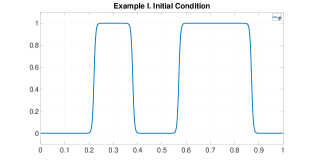
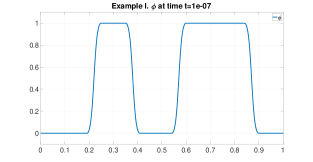
Figure 3: Example I. Left: Initial condition $\phi_{0}(x)$ at $t=0$. Right: $\phi(x,t)$ at $t=10^{-7}$.

In all the simulations in this section we have considered the time interval $[0,T]=[0,10^{-7}]$ and time step $\Delta t=10^{-10}$. The expected dynamic of the system is that the pure phases $\phi=0$ and $\phi=1$ will not merge in a larger pure phase region because they are too far apart to interact between them, in fact they will just accommodate the width of the interface to reach an equilibrium. This dynamic is completely different from the one associated with constant mobility, where the two pure phases will end up forming larger regions due to the coarsening effects.

We have separated the presentation of the results into two parts: first we present the comparison of the three schemes with fixed values of $\eta$ and $\varepsilon$ while varying the size of the spatial discretization, with $N(=h^{-1})$ denoting the number of points in the (equally distributed) spatial mesh. In the second step we compare the G_ε and J_ε schemes with fixed value of $N$ and varying the values of $\eta$ and $\varepsilon$ in order to see if the estimates derived in Lemmas 1 and 2 become apparent in our numerical experiments.

4.3.1 Comparison of G_ε, J_ε and M₀ schemes. Fixed $\eta=0.005$ and $\varepsilon=10^{-20}$

In Figure 4 we present comparisons of the evolution in time of the maximum and minimum of $\phi$ for each scheme when different size of the discretization of the spatial mesh is considered (i.e. different values of the number of points $N$). In particular, since $\eta=0.005$ we focus on cases such that $N\geq 200$, hence $h\leq\eta$.

We can observe how M₀-scheme is always much less effective in maintaining the values of $\phi$ inside the interval $[0,1]$ than the G_ε and J_ε schemes. Moreover, the larger $N$ the better the behavior of M₀-scheme with respect to the boundedness of $\phi$, achieving equivalent performance to the G_ε and J_ε schemes only for the demanding requirement $N\geq 10^{4}$. This fact is expected because taking $h$ to zero we are getting closer to the only discrete in time version of scheme (45), which satisfies the boundedness estimates.

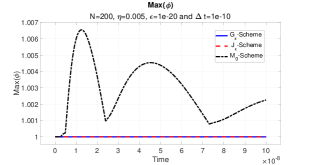
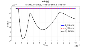
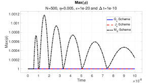
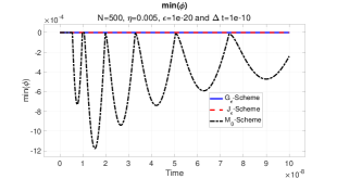
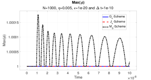
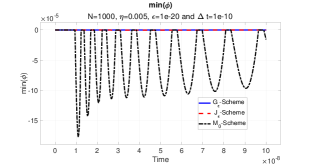
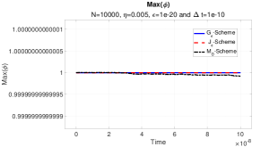
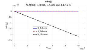
Figure 4: Example I. Evolution in time of $\max(\phi)$ (left column) and $\min(\phi)$ (right column) for G_ε-scheme, J_ε-scheme and M₀-scheme considering $N=200,500,1000$ and $10000$ (from top to bottom).

4.3.2 Study of the influence of $\eta$ and $\varepsilon$ in the boundedness estimates (fixed $N=10^{4}$ and $\Delta t=10^{-10}$)

We present in Tables 1 and 2 the results obtained using G_ε and J_ε schemes with different values of $\eta$ and $\varepsilon$. For $\eta=0.01$ (the largest value of $\eta$ considered) both schemes achieve $\phi<1$ and very small negative values of $\phi$ when $\varepsilon\leq 10^{-3}$. Decreasing the value of $\eta$ from $\eta=0.01$ to $\eta=0.005$ produces that the value of $\varepsilon$ needed to achieve equivalent sharpness of the bounds also decreases, in particular, it is needed to consider $\varepsilon\leq 10^{-4}$ with $\eta=0.075$ and $\varepsilon\leq 10^{-5}$ with $\eta=0.005$ for both schemes. The main difference here is that larger values of $\varepsilon$ using G_ε-scheme result in no reliable simulations (for some of the larger values of $\varepsilon$ the iterative algorithm does not even converge). On the other hand, for J_ε-scheme the obtained results are not as sharp as for smaller values of $\varepsilon$, although convergence of the algorithm is achieved in all cases. The different convergence behavior for both schemes can be explained by the boundedness estimates in Corollaries 1 and 2, because the bounds for G_ε-scheme degenerate as $\eta$ decreases while the bounds for J_ε-scheme are independent of $\eta$ .

When the value of $\eta$ is reduced even further the situation become more challenging, because a smaller value of $\eta$ results in a narrower interface thickness while using the same discretization parameters $N=10^{4}$ and $\Delta t=10^{-10}$. For the cases $\eta=0.0025$ and $\eta=0.001$, G_ε-scheme needs to consider $\varepsilon\leq 10^{-6}$ to be reliable (again for some of the larger values of $\varepsilon$ the iterative algorithm does not converge). By comparison, J_ε-scheme seems to be much more reliable in these situations for $\varepsilon\leq 10^{-2}$, although the obtained bounds in J_ε-scheme are not as sharp as the ones obtained with larger values $\eta$.

The results of these numerical experiments corroborate that the boundedness estimates for both schemes improve when considering lower values of $\varepsilon$ and in the case of G_ε-scheme the truncation parameter $\varepsilon$ should be smaller than $\eta^{2}$ to be effective.

G${}_{\varepsilon}(\phi)$	$\eta=0.01$		$\eta=0.0075$		$\eta=0.005$
$\varepsilon$	$\displaystyle\max_{t\in[0,T]}\max_{x\in\Omega}\phi$	$\displaystyle\min_{t\in[0,T]}\min_{x\in\Omega}\phi$	$\displaystyle\max_{t\in[0,T]}\max_{x\in\Omega}\phi$	$\displaystyle\min_{t\in[0,T]}\min_{x\in\Omega}\phi$	$\displaystyle\max_{t\in[0,T]}\max_{x\in\Omega}\phi$	$\displaystyle\min_{t\in[0,T]}\min_{x\in\Omega}\phi$
$10^{-2}$	$1.00001$	$-1.9\times 10^{-3}$	$1.0004$	$-6.0\times 10^{-3}$	$1.0033$	$-7.05\times 10^{-3}$
$10^{-3}$	$0.99999$	$-3.07\times 10^{-14}$	$\times$	$\times$	$\times$	$\times$
$10^{-4}$	$0.99999$	$-3.07\times 10^{-14}$	$0.99999$	$-7.33\times 10^{-18}$	$\times$	$\times$
$10^{-5}$	$0.99999$	$-3.07\times 10^{-14}$	$0.99999$	$-5.79\times 10^{-18}$	$1.0+10^{-14}$	$-6.73\times 10^{-18}$
$10^{-6}$	$0.99999$	$-3.07\times 10^{-14}$	$0.99999$	$-5.85\times 10^{-18}$	$1.000000$	$-5.81\times 10^{-18}$
$10^{-7}$	$0.99999$	$-3.07\times 10^{-14}$	$0.99999$	$-5.76\times 10^{-18}$	$1.000000$	$-5.84\times 10^{-18}$
$10^{-8}$	$0.99999$	$-3.07\times 10^{-14}$	$0.99999$	$-5.72\times 10^{-18}$	$1.000000$	$-5.72\times 10^{-18}$

G${}_{\varepsilon}(\phi)$	$\eta=0.0025$		$\eta=0.001$
$\varepsilon$	$\displaystyle\max_{t\in[0,T]}\max_{x\in\Omega}\phi$	$\displaystyle\min_{t\in[0,T]}\min_{x\in\Omega}\phi$	$\displaystyle\max_{t\in[0,T]}\max_{x\in\Omega}\phi$	$\displaystyle\min_{t\in[0,T]}\min_{x\in\Omega}\phi$
$10^{-2}$	$1.024$	$-6.9\times 10^{-3}$	$\times$	$\times$
$10^{-3}$	$1.0008$	$-2.0\times 10^{-3}$	$\times$	$\times$
$10^{-4}$	$\times$	$\times$	$\times$	$\times$
$10^{-5}$	$1.0943$	$-5.6\times 10^{-5}$	$1.0244$	$-6.38\times 10^{-5}$
$10^{-6}$	$1.000009$	$-9.72\times 10^{-6}$	$1.0007$	$-1.08\times 10^{-5}$
$10^{-7}$	$1.0000014$	$-1.43\times 10^{-6}$	$1.000024$	$-6.07\times 10^{-6}$
$10^{-8}$	$1.0000012$	$-1.26\times 10^{-6}$	$1.000006$	$-6.73\times 10^{-6}$

Table 1: Example I. G_ε-scheme. Evolution in time of the minimum and maximum values achieved by $\phi$ in the domain $\Omega$ in the whole interval $[0,T]$ for different values of $\eta$ and $\varepsilon$ with fixed values of the discretization parameters $N=10000$ and $\Delta t=10^{-10}$. Symbol $\times$ denotes that at some point the iterative method did not converge.

J${}_{\varepsilon}(\phi)$	$\eta=0.01$		$\eta=0.0075$		$\eta=0.005$
$\varepsilon$	$\displaystyle\max_{t\in[0,T]}\max_{x\in\Omega}\phi$	$\displaystyle\min_{t\in[0,T]}\min_{x\in\Omega}\phi$	$\displaystyle\max_{t\in[0,T]}\max_{x\in\Omega}\phi$	$\displaystyle\min_{t\in[0,T]}\min_{x\in\Omega}\phi$	$\displaystyle\max_{t\in[0,T]}\max_{x\in\Omega}\phi$	$\displaystyle\min_{t\in[0,T]}\min_{x\in\Omega}\phi$
$10^{-2}$	$1.00195$	$-1.9\times 10^{-3}$	$1.00594$	$-5.94\times 10^{-3}$	$1.00693$	$-6.93\times 10^{-3}$
$10^{-3}$	$0.999999$	$-3.7\times 10^{-14}$	$1.00112$	$-1.12\times 10^{-3}$	$1.00201$	$-2.01\times 10^{-3}$
$10^{-4}$	$0.999999$	$-3.7\times 10^{-14}$	$0.999999$	$-7.31\times 10^{-18}$	$1.00022$	$-2.26\times 10^{-4}$
$10^{-5}$	$0.999999$	$-3.7\times 10^{-14}$	$0.999999$	$-5.79\times 10^{-18}$	$1.0+7\times 10^{-15}$	$-6.73\times 10^{-18}$
$10^{-6}$	$0.999999$	$-3.7\times 10^{-14}$	$0.999999$	$-5.85\times 10^{-18}$	$1.00000$	$-5.81\times 10^{-18}$
$10^{-7}$	$0.999999$	$-3.7\times 10^{-14}$	$0.999999$	$-5.76\times 10^{-18}$	$1.00000$	$-5.84\times 10^{-18}$
$10^{-8}$	$0.999999$	$-3.7\times 10^{-14}$	$0.999999$	$-5.72\times 10^{-18}$	$1.00000$	$-5.72\times 10^{-18}$

J${}_{\varepsilon}(\phi)$	$\eta=0.0025$		$\eta=0.001$
$\varepsilon$	$\displaystyle\max_{t\in[0,T]}\max_{x\in\Omega}\phi$	$\displaystyle\min_{t\in[0,T]}\min_{x\in\Omega}\phi$	$\displaystyle\max_{t\in[0,T]}\max_{x\in\Omega}\phi$	$\displaystyle\min_{t\in[0,T]}\min_{x\in\Omega}\phi$
$10^{-2}$	$1.00679$	$-6.79\times 10^{-3}$	$1.0044$	$-0.0044$
$10^{-3}$	$1.00203$	$-2.03\times 10^{-3}$	$1.0017$	$-0.0017$
$10^{-4}$	$1.00033$	$-3.39\times 10^{-4}$	$1.0004$	$-3.66\times 10^{-4}$
$10^{-5}$	$1.000054$	$-5.45\times 10^{-5}$	$1.0001$	$-6.47\times 10^{-5}$
$10^{-6}$	$1.000009$	$-9.7\times 10^{-6}$	$1.000012$	$-1.207\times 10^{-5}$
$10^{-7}$	$1.000001$	$-1.43\times 10^{-6}$	$1.000015$	$-1.58\times 10^{-5}$
$10^{-8}$	$1.000001$	$-1.25\times 10^{-6}$	$1.0000088$	$-8.81\times 10^{-6}$

Table 2: Example I. J_ε-scheme. Evolution in time of the minimum and maximum values achieved by $\phi$ in the domain $\Omega$ in the whole interval $[0,T]$ for different values of $\eta$ and $\varepsilon$ with fixed values of the discretization parameters $N=10000$ and $\Delta t=10^{-10}$.

4.4 Example II. Accuracy study

In this second example we estimate numerically the order of convergence in space of the presented numerical schemes. We consider the parameters values $\eta=0.005$ and $\varepsilon=10^{-20}$. We now introduce some additional notation. The individual errors using discrete norms and the convergence rate between two spatial meshes of size $h$ and $\widetilde{h}$ are defined as

$$e_{2}(\phi):=\|\phi_{exact}-\phi_{h}\|_{L^{2}(\Omega)}\,,\quad\mbox{ and }\quad r_{2}(\phi):=\left[\log\left(\frac{e_{2}(\phi)}{\tilde{e}_{2}(\phi)}\right)\right]\Big{/}\left[\log\left(\frac{h}{\widetilde{h}}\right)\right]\,.$$

We consider the time step set to $\Delta t=10^{-10}$ and the time interval $[0,T]=[0,10^{-7}]$. The initial configuration $\phi_{0}$ is determined by (46), the same configuration that was used in Example I (initial and final configuration of $\phi$ are presented in Figure 3). We have considered this challenging configuration where there are regions with $\phi=0$ and $\phi=1$. We compute the EOC using as reference (or exact) solution the one obtained by solving the system using the spatial mesh size $h=10^{-5}$ using G_ε-scheme. The errors and orders of convergence are presented in Table 3. The results from the two experiments show that G_ε-scheme and J_ε-scheme achieve the optimal order of $\mathcal{O}(h^{2})$ as the classical $M_{0}(\phi)$-scheme, that is, the construction of the proposed boundedness preserving numerical schemes do not cause to lose order of convergence.

	Gε-Scheme		Jε-Scheme		M0-Scheme
$N(=h^{-1})$	$e_{2}(\phi)$	$r_{2}(\phi)$	$e_{2}(\phi)$	$r_{2}(\phi)$	$e_{2}(\phi)$	$r_{2}(\phi)$
$2000$	$0.000013314$	$-$	$0.000008683$	$-$	$0.000009283$	$-$
$3000$	$0.000005907$	$2.004047$	$0.000003863$	$1.997343$	$0.000004086$	$2.024024$
$4000$	$0.000003330$	$1.992257$	$0.000002192$	$1.970207$	$0.000002309$	$1.982729$
$5000$	$0.000002142$	$1.976693$	$0.000001416$	$1.957809$	$0.000001494$	$1.950956$
$6000$	$0.000001500$	$1.953188$	$0.000000990$	$1.963118$	$0.000001053$	$1.917623$

Table 3: Example II. Experimental absolute errors and accuracy order.

4.5 Example III. Spinodal decomposition

In this example we illustrate the validity of the schemes to capture realistic dynamics. To this end we have only used G_ε-scheme with parameter $\varepsilon=10^{-20}$, because we have seen in Example I that with this choice of the truncation parameter both schemes G_ε and J_ε behaves equivalently. The time interval is $[0,10^{-3}]$ and the rest of the considered parameters are $\eta=0.005$, $N=10^{3}$ and $\Delta t=10^{-8}$ We have simulated a spinodal decomposition dynamics, that is, we consider initially that the two components of our system are very mixed by taking as initial condition a random perturbation of amplitude $0.01$ of the constant value $\phi=0.5$. In order to decrease the energy of the system, the dynamics are expected to pull the values of $\phi$ close to the end points of the interval $[0,1]$ and at the same time try to reduce the amount of interface in the system. We can observe in Figure 5 how the results of our simulations correspond with the expected dynamics. Moreover we can observe in Figure 6 the evolution in time of: the energy (always decreasing), the volume (always constant), $\displaystyle\max_{x\in\Omega}\phi$ (always $\leq 1$) and $\displaystyle\min_{x\in\Omega}\phi$ (always $\geq 0$), in fact in this example

$$\max_{t\in[0,10^{-3}]}\max_{x\in\Omega}\phi=0.999624\quad\quad\quad\mbox{ and }\quad\quad\quad\min_{t\in[0,10^{-3}]}\min_{x\in\Omega}\phi=1.58\times 10^{-4}\,.$$

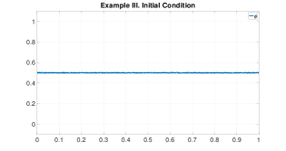
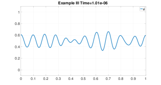
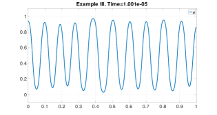
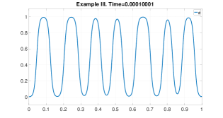
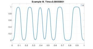
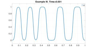
Figure 5: Example III. Evolution in time of $\phi$ for G_ε-scheme

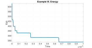
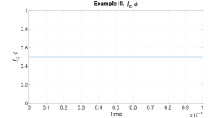
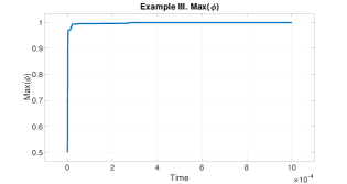
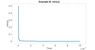
Figure 6: Example III. Evolution in time of: $E(\phi)$ (top left), $\int_{\Omega}\phi dx$ (top right), $\max(\phi)$ (bottom left) and $\min(\phi)$ (bottom right).

4.6 Example IV. Spinodal decomposition in $2D$

In this section we perform simulations in the two dimensional domain $\Omega=[0,1]\times[0,1]$ in order to evidence that the effective implementation of the code in higher dimension can be performed in structured meshes and to compare the different dynamics obtained using constant and non-constant mobilities. To this end we have compared G_ε-scheme and J_ε-scheme (both with parameter $\varepsilon=10^{-8}$ and non-constant mobility) with M₀-scheme (45) (with constant mobility $M_{0}(\phi)=1$). The time interval is $[0,5\times 10^{-5}]$ and the rest of the considered parameters are $\eta=0.01$, $N=10^{2}$ and $\Delta t=10^{-9}$. As in the previous example, we have considered initially that the two components of our system are very mixed by taking as initial condition a random perturbation of amplitude $0.01$ of the constant value $\phi=0.5$ to simulate a spinodal decomposition dynamic. The dynamics of the three simulations are presented in Figure 7, and we can observe (as expected) that the separation process occurs faster in the case of considering a constant mobility (this fact is also illustrated in the results presented in [10]).

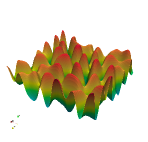
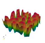
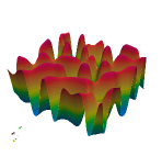
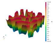
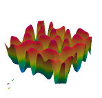
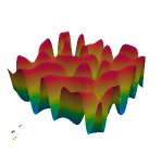
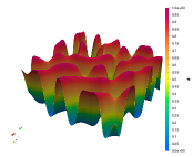
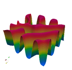
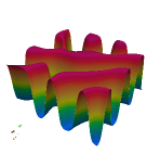
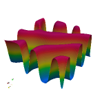
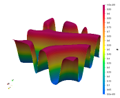
Figure 7: Example IV. Evolution in time (from left to right) of $\phi$ at times $t=2\times 10^{-5},3\times 10^{-5},4\times 10^{-5}$ and $5\times 10^{-5}$. Top row: G_ε-scheme. Middle row: J_ε-scheme. Bottom row: Scheme with $M(\phi)=1$.

5 Conclusions

In this work we have derived two new numerical schemes to approximate the Cahn-Hilliard equation with degenerate mobility. The main ideas to derive the schemes are to first truncate the mobility term away from the values $\varepsilon$ and $1-\varepsilon$ and then realize that apart of the classical energy law, the system also satisfy estimates for singular potentials which can be used to derive estimates about the boundedness of the variable $\phi$ in terms of the truncation parameter $\varepsilon$. In particular, the derived estimates for each of the numerical schemes are associated to different singular potentials.

The resulting numerical schemes have been implemented and compared with the standard approach of truncating the mobility by zero (to avoid negative flux even if $\phi$ goes outside of the interval $[0,1]$) and it has been shown that the new schemes behave much better in terms of achieving the desired bounds for $\phi$. Moreover, the new schemes have been shown to obtain optimal order of convergence and to be able to capture the most challenging of the benchmarks for the Cahn-Hilliard equation, that is, to simulate properly the spinodal decomposition in one and two dimensions, evidencing that these ideas are valid independently of the spatial dimension.

References

- [1] Acosta-Soba, D., Guillén-González, F. & Rodríguez-Galván, J.R. 2023 An upwind DG scheme preserving the maximum principle for the convective Cahn-Hilliard model. Numerical Algorithms 92, 1589-1619.
- [2] Bates, P.W. & Fife, P.C. 1993 The dynamics of nucleation for the Cahn-Hilliard equation. SIAM J Appl Math 53, 990-1008.
- [3] Barrett, J.W., Blowey, J.F. & Garcke, H. 1998 Finite element approximation of a fourth order nonlinear degenerate parabolic equation. Numer. Math. 80, 525-556.
- [4] Caffarelli, L.A. & Muler, N.E. 1995 An L∞ Bound for Solutions of the Cahn-Hilliard Equation. Arch. Rational Mech. Anal. 133, 129-144.
- [5] Cahn, J.W. & Hilliard, J.E. 1958 Free energy of a nonuniform system. I. Interfacial free energy. J. Chem. Phys. 28, 258-267.
- [6] Ciarlet, P.G. & Raviart, P.A. 1973 Maximum principle and uniform convergence for the finite element method. Comput. Methods Appl. Mech. Engrg. 2, 17-31.
- [7] Copetti, M.I.M. & Elliot, C.M. 1992 Numerical analysis of the Cahn-Hilliard equation with a logarithmic free energy. Numer. Math. 63, 39-65.
- [8] Dai, S. & Du, Q. 2012 Motion of interfaces governed by the Cahn-Hilliard equation with highly disparate diffusion mobility. SIAM J. Appl. Math. 72, 1818-1841.
- [9] Dai, S. & Du, Q. 2014 Coarsening mechanism for systems governed by the Cahn-Hilliard equation with degenerate diffusion mobility. Multiscale Modeling Simul. 12, 1870-1889.
- [10] Dai, S. & Du, Q. 2016 Computational studies of coarsening rates for the Cahn-Hilliard equation with phase-dependent diffusion mobility. Journal of Computational Physics 310, 85-108.
- [11] Dai, S. & Du, Q. 2016 Weak Solutions for the Cahn-Hilliard Equation with Degenerate Mobility. Archive for Rational Mechanics and Analysis 219, 1161-1184.
- [12] Elliot, C.M. & Garcke, H. 1996 On the Cahn-Hilliard equation with degenerate mobility. SIAM J. Math. Anal 27, 404-423.
-
[13]
Eyre, D.J.
An Unconditionally Stable One-Step Scheme for Gradient System,
http://www.math.utah.edu/ eyre/research/methods/stable.ps, unpublished. - [14] Guillén-González, F., Rodríguez-Bellido, M.A. & Rueda-Gómez D.A. Unconditionally energy stable fully discrete schemes for a chemo-repulsion model Mathematics of Computation 88 (2019) 2069-2099.
- [15] Guillén-González, F., Rodríguez-Bellido, M.A. & Rueda-Gómez, D.A. Study of a chemorepulsion model with quadratic production. Part II: Analysis of an unconditional energystable fully discrete scheme. Computers and Mathematics with Applications, 80 (2020) 636- 652.
- [16] Guillén-González, F., Rodríguez-Bellido, M.A. & Rueda-Gómez, D.A.; A chemorepulsion model with superlinear production: analysis of the continuous problem and two approximately positive and energy-stable schemes. Advances in Comput. Math. 47-6, Springer, (2021).
- [17] Guillén-González, F., Rodríguez-Bellido, M.A. & Rueda-Gómez, D.A.; Comparison of two finite element schemes for a chemo-repulsion system with quadratic production. Applied Numerical Mathematics. 173, pp. 193-210. (2022).
-
[18]
Guillén-González, F. & Tierra G.
Finite Element numerical schemes for a chemo-attraction and consumption model.
Submitted
https://arxiv.org/abs/2112.03431 - [19] Hecht, F. 2012 New development in FreeFem++. J. Numer. Math. 20, 251-265.
- [20] Kay, D., Styles, V. & Süli E. 2009 Discontinuous Galerkin finite element approximation of the Cahn-Hilliard equation with convection. SIAM J. Numer. Anal. 47 2660-2685.
- [21] A. A. Lee, A. Munch, and E. Süli. 2015 Degenerate mobilities in phase field models are insufficient to capture surface diffusion. Applied Physics Letters 107, 081603.
- [22] A. A. Lee, A. Munch, and E. Süli. 2016 Sharp-interface limits of the Cahn-Hilliard equation with degenerate mobility. SIAM J. Appl. Math. 76, 433-456.
- [23] A. A. Lee, A. Munch, and E. Süli. 2016 Response to "Comment on ’Degenerate mobilities in phase field models are insufficient to capture surface diffusion’". Applied Physics Letters 108, 036102.
- [24] Liu, C., Frank, F. & Rivière B.M. 2019 Numerical error analysis for nonsymmetric interior penalty discontinuous Galerkin method of Cahn-Hilliard equation. Numer. Methods Partial Differential Equations 35 1509-1537.
- [25] MATLAB R2021b version 9.11.0. Natick, Massachusetts: The MathWorks Inc. (2021)
- [26] Nochetto, R.H., Salgado, A.J. & Walker S.W. 2014 A Diffuse Interface Model for Electrowetting with Moving Contact Lines. Mathematical Models and Methods in Applied Sciences 24 67-111.
- [27] Novick-Cohen, A.,& Segel, L.A. 1984 Nonlinear aspects of the Cahn-Hilliard equation. Phys D 10 277-298.
- [28] Salgado, A.J. 2012 A diffuse interface fractional time-stepping technique for incompressible two-phase flows with moving contact lines M2AN Math. Model. Numer. Anal. 31, 743-758.
- [29] Shen, J. & Yang, X. 2010 Energy stable schemes for Cahn-Hilliard phase-field model of two-phase incompressible flows Chin. Ann. Math. Ser. B 31, 743-758.
- [30] Tierra, G. & Guillén-González, F. 2015 Numerical methods for solving the Cahn-Hilliard equation and its applicability to related energy-based models. Arch. Comput. Methods Eng. 22, 269-289.
- [31] A. Voigt. 2016 Comment on "Degenerate mobilities in phase field models are insufficient to capture surface diffusion" [Appl. Phys. Lett. 107, 081603(2015)]. Applied Physics Letters 108, 036101.
- [32] van der Waals, J.D. 1893 The thermodynamic theory of capillarity flow under the hypothesis of a continuous variation of density. Verhandel. Konink. Akad. Weten. Amsterdam 1.
- [33] Wu, X., van Zwieten, G.J. & van der Zee, K.G. 2014 Stabilized second-order convex splitting schemes for Cahn-Hilliard models with application to diffuse-interface tumor-growth models Int. J. Numer. Meth. Biomed. Engng. 30, 180-203.
- [34] Xia, Y., Xu, Y. & Shu, C.-W. 2007 Local discontinuous Galerkin methods for the Cahn-Hilliard type equations J. Comput. Phys. 227, 472-491.