Centroid Adapted Frequency Selective Extrapolation
for Reconstruction of Lost Image Areas

Abstract

Lost image areas with different size and arbitrary shape can occur in many scenarios such as error-prone communication, depth-based image rendering or motion compensated wavelet lifting. The goal of image reconstruction is to restore these lost image areas as close to the original as possible. Frequency selective extrapolation is a block-based method for efficiently reconstructing lost areas in images. So far, the actual shape of the lost area is not considered directly. We propose a centroid adaption to enhance the existing frequency selective extrapolation algorithm that takes the shape of lost areas into account. To enlarge the test set for evaluation we further propose a method to generate arbitrarily shaped lost areas. On our large test set, we obtain an average reconstruction gain of 1.29 dB.

I Introduction

Image reconstruction aims at restoring lost areas in images as close as possible to the original. There are several applications where lost areas of arbitrary shape can occur and need to be reconstructed, e.g., when distortions like scratches or dust are to be removed from scanned images. In multiview scenarios, lost areas can occur especially at object boundaries, when an intermediate view is computed by depth-image based rendering [1]. In motion compensated frame rate up conversion [2], lost areas can occur in predicted intermediate frames. A very similar pattern of lost areas occurs when the block-based motion compensation is inverted, e.g., in the update step of compensated wavelet lifting, unconnected pixels can occur [3]. In [4], the reconstruction of these unconnected pixels was shown to be advantageous. In all of these applications, the different size and the arbitrary shape of the occurring lost areas is challenging.

Several methods exist for reconstructing lost image areas. In [5], classical kernel regression (CKR) is extended by nonlinear kernel adaption to obtain steering kernel regression (SKR). [6] proposes a framework based on total variation (TV) that can be used for reconstructing larger lost areas in images, e.g., to remove text overlays. In [7], the constraint split augmented Lagrangian shrinkage algorithm (CSALSA) is proposed and used for reconstructing images with lost pixels. The frequency selective extrapolation (FSE) generates a model in the frequency domain based on the available pixels [8].

In natural images, pixels closer to each other have a higher correlation. The correlation reduces with increasing distance of the pixels. When some pixels are lost, support pixels closer to these lost pixels should have a higher influence on the reconstruction. FSE is a block-based method which uses an isotropic weighting function to control the influence of the support pixels. So far, mostly block losses were considered where the currently considered block was completely lost, i.e., the weighting function is centered w.r.t. the currently considered block.

In this paper, we focus on the reconstruction of images with arbitrarily shaped lost areas. We propose a centroid adaption of FSE (CA-FSE) to address the arbitrary shape of lost areas. To evaluate the performance, we propose a method to simulate the arbitrarily shaped lost areas occurring in the above mentioned scenarios. Fig. 1 shows an example image with dense and sparse loss pattern. By applying different loss patterns to different images, the performance of the reconstruction methods is evaluated and compared on a very large test set.

In Section II, we briefly review the FSE algorithm and introduce our proposed centroid adaption in Section III. Simulation results and discussion follow in Section IV.

Original	Dense loss pattern		Sparse loss pattern

Figure 1: Detail of an image, arbitrarily shaped loss patterns (black is lost), and images to be reconstructed

II Frequency Selective Extrapolation

Frequency selective extrapolation (FSE) [8] is a block-based iterative method for reconstructing lost areas in images. With the optimized processing order [9], the size of lost areas is taken into account. The more available support pixels a block has, the earlier it is processed and bigger lost areas are processed from the border to the center. However, in contrast to the size, the shape of the lost areas is not considered so far.

For every block, FSE generates a model

$$g\left[m,n\right]=\sum_{k\in\mathcal{K}}\hat{c}_{k}\varphi_{k}\left[m,n\right]$$

for the unknown pixels based on the available pixels in the support area. A weighted superposition of 2-D Fourier basis functions $\varphi_{k}$ is generated where the set $\mathcal{K}$ contains the indexes of all basis functions. In every iteration, the influence $\hat{c}_{k}$ of the basis function $\varphi_{k}$ is increased that reduces the approximation error the most.

\psfragscanon\psfrag{tag0}{Pixel categories of $\mathcal{L}$:}\psfrag{tag1}{originally known $\mathcal{A}$ }\psfrag{tag2}{already reconstructed $\mathcal{R}$}\psfrag{tag3}{$\mathcal{B}_{o}$: lost, outside of $\mathfrak{b}$}\psfrag{tag4}{$\mathcal{B}_{i}$: lost, inside of $\mathfrak{b}$}\psfrag{tag5}{$\mathcal{L}=\mathcal{A}\cup\mathcal{R}\cup\mathcal{B}_{i}\cup\mathcal{B}_{o}$}\psfrag{m}{$m$}\psfrag{n}{$n$}\psfrag{b}{$\mathfrak{b}$}\psfrag{d}{$d$}\includegraphics[width=208.13574pt]{img/skizze_areas}

\psfragscanon\psfrag{tag0}{Pixel categories of $\mathcal{L}$:}\psfrag{tag1}{originally known $\mathcal{A}$ }\psfrag{tag2}{already reconstructed $\mathcal{R}$}\psfrag{tag3}{$\mathcal{B}_{o}$: lost, outside of $\mathfrak{b}$}\psfrag{tag4}{$\mathcal{B}_{i}$: lost, inside of $\mathfrak{b}$}\psfrag{tag5}{$\mathcal{L}=\mathcal{A}\cup\mathcal{R}\cup\mathcal{B}_{i}\cup\mathcal{B}_{o}$}\psfrag{m}{$m$}\psfrag{n}{$n$}\psfrag{b}{$\mathfrak{b}$}\psfrag{d}{$d$}\psfragscanon\includegraphics[width=208.13574pt]{img/skizze_areas_beschriftung}

Figure 2: Composition of extrapolation area $\mathcal{L}$. The corresponding weighting functions are shown in Fig. 3.

Fig. 2 shows the composition of the extrapolation area $\mathcal{L}$. The area $\mathcal{L}$ has a size of $M\times N$ pixels and consists of the currently considered block $\mathfrak{b}$ in the center, surrounded by a support area of width $d$. The pixels within $\mathcal{L}$ come from three categories, namely originally known pixels $\mathcal{A}$, already reconstructed pixels $\mathcal{R}$ and lost pixels $\mathcal{B}_{i}\cup\mathcal{B}_{o}$ that have not been reconstructed so far. Thereby, $\mathcal{B}_{i}$ contains lost pixels within the currently considered block $\mathfrak{b}$ and $\mathcal{B}_{o}$ contains lost pixels outside of $\mathfrak{b}$, respectively. Lost pixels within the currently considered block $\mathfrak{b}$ are reconstructed by an inverse transform of the model $g$. For a more detailed description of FSE together with pseudo code, please refer to [8, 9].

III Proposed Centroid Adaption

To control the influence of the support pixels during the model generation, a weighting function $w\left[m,n\right]$ is used. The influence decreases with increasing distance to the center of $\mathfrak{b}$. The weighting function is computed to

$$w\left[m,n\right]=\begin{cases}\rho^{\sqrt{\left(m-\bar{m}\right)^{2}+\left(n-\bar{n}\right)^{2}}}&\text{for }\left[m,n\right]\in\mathcal{A}\\ \delta\rho^{\sqrt{\left(m-\bar{m}\right)^{2}+\left(n-\bar{n}\right)^{2}}}&\text{for }\left[m,n\right]\in\mathcal{R}\\ 0&\text{for }\left[m,n\right]\in\mathcal{B}_{i}\cup\mathcal{B}_{o}\end{cases}$$ (1)

where $\left[\bar{m},\bar{n}\right]$ is the center of the block $\mathfrak{b}$. On the left of Fig. 3, an example is shown with $w\left[m,n\right]$ centered in $\mathfrak{b}$ corresponding to the areas named in Fig. 2. The decay is controlled by $\rho$ and the weight of already reconstructed pixels $\mathcal{R}$ is attenuated by $\delta$.

So far, mostly block losses were considered where $\mathfrak{b}$ was completely lost. Especially for arbitrarily shaped lost areas, the case occurs quite often where only a part of the reconstruction area is actually lost.

The weighting function $w\left[m,n\right]$ controls the influence of the support pixels on the model generation. Support pixels closer to the lost area shall have more influence than pixels farther away. So far, the weighting function does not consider the case that only a part of the pixels within $\mathfrak{b}$ can be lost. To adapt the model generation to the arbitrary shape of the lost area, we propose to center the weighting function on the centroid of the lost pixels $\mathcal{B}_{i}$, i.e., within $\mathfrak{b}$. The proposed weighting function is computed by

$$w\left[m,n\right]=\begin{cases}\rho^{\sqrt{\left(m-m_{c}\right)^{2}+\left(n-n_{c}\right)^{2}}}&\text{for }\left[m,n\right]\in\mathcal{A}\\ \delta\rho^{\sqrt{\left(m-m_{c}\right)^{2}+\left(n-n_{c}\right)^{2}}}&\text{for }\left[m,n\right]\in\mathcal{R}\\ 0&\text{for }\left[m,n\right]\in\mathcal{B}_{i}\cup\mathcal{B}_{o}\end{cases}$$ (2)

where the centroid $\left[m_{c},n_{c}\right]$ of the lost pixels $\mathcal{B}_{i}$ within the block $\mathfrak{b}$ is computed by

$$m_{c}=\frac{1}{\left|\mathcal{B}_{i}\right|}\sum_{\forall m\in\mathcal{B}_{i}}m n_{c}=\frac{1}{\left|\mathcal{B}_{i}\right|}\sum_{\forall n\in\mathcal{B}_{i}}n$$

On the right of Fig. 3, an example for centering $w\left[m,n\right]$ on the centroid of the lost pixels within $\mathfrak{b}$ is shown. This leads to the intended weighting of the pixels with respect to the distance of the actual lost area. In the following, the centroid adapted FSE is called CA-FSE.

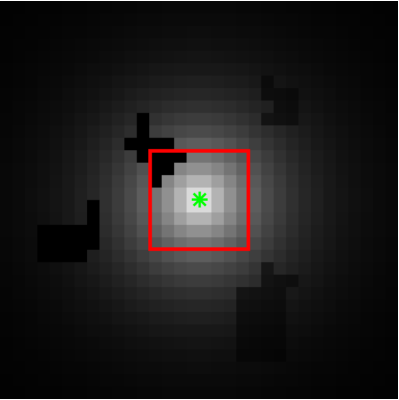
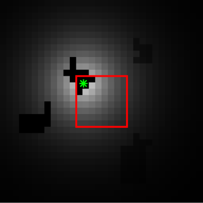
Figure 3: Example for moving the center (marked by a green star) of the weighting function $w\left[m,n\right]$ to the centroid of the lost pixels (black) within the currently considered block $\mathfrak{b}$ (red box). The different kinds of pixels are labeled in Fig. 2. Left: $w\left[m,n\right]$ centered in the currently considered block $\mathfrak{b}$, Right: $w\left[m,n\right]$ centered on the centroid of the lost pixels inside the currently considered $\mathfrak{b}$

IV Simulation Results and Analysis

For evaluation, we used the images from the two image databases Tecnick [10], consisting of 100 images of size $1200\times 1200$, and Kodak [11], consisting of 24 images of size $512\times 768$. To extend our test set, we took the first image of each sequence of the ARRI database [12]. We further took views 0 from Illumination 1 and Exposure 1 of the Middleburry multiview databases from 2005, 2006, and 2014 [13, 14, 15]. The luminance of each image was used.

We used three typical parameter sets for FSE and CA-FSE, called ‘bs 4’, ‘bs 8’, and ‘bs 16’ listed in Tab. I.

Table I: FSE parameter sets.

FSE parameter set denoted as	bs 4	bs 8	bs 16
size of block $\mathfrak{b}$	$4\times 4$	$8\times 8$	$16\times 16$
border width $d$ around $\mathfrak{b}$	14	12	16
FFT size	32	32	64
decay parameter for $w\left[m,n\right]$	$\rho=0.7$
attenuated weight for $\mathcal{R}$	$\delta=0.5$
orthogonality correction $\gamma$	$\gamma=0.5$

Figure 4: Difference PSNR in dB of the reconstructed pixels between the centroid adaption (CA-FSE) and the unmodified weighting function (FSE) for a dense loss pattern, Left: Kodak, Right: Tecnick.

For the simulation, the loss patterns are generated using the following commands in MATLAB

$$\mathtt{dense\_loss\text{\_}pattern}=\mathtt{imdilate(rand(img\text{\_}size)>0.98,}\\ \mathtt{strel(\text{'}square\text{'},8));}$$ (3)

$$\mathtt{sparse\_loss\text{\_}pattern}=\mathtt{imdilate(rand(img\text{\_}size)>0.95,}\\ \mathtt{strel(\text{'}square\text{'},8));}$$ (4)

Visual examples for the two loss patterns are shown in Fig. 1. Lost pixels are colored in black. The dense loss pattern in (3) causes a loss of about 28% of pixels and the sparse loss pattern in (4) about 4%, respectively. The challenging patterns are very similar to the lost areas that occur in different applications. We choose the dense pattern to evaluate the algorithms on larger lost areas.

For both loss pattern types, the simulations were repeated for 10 different loss patterns to obtain significant results and to avoid special effects from a single specific pattern. For each loss pattern, the PSNR is computed on the reconstructed pixels only. Then, for each loss pattern, the average is computed for the 10 different loss patterns. Fig. 4 shows the results for the Kodak and the Tecnick database for the dense loss pattern. Whenever the difference is positive, CA-FSE obtains a better reconstruction result. The dotted lines show the average result for each test set. The corresponding values to the dotted lines are listed as diff in the first two lines of Tab. IV together with the absolute PSNR values. In the lower part, Tab. IV contains the corresponding averaged results of the simulation using the sparse loss pattern. Further, both tables contain results from four recent reference methods from the literature, namely based on kernel regression (CKR) and (SKR) [5], total variation (TV) [6], and constraint lagrangian shrinkage (CSALSA) [7].

Table II: Averaged PSNR values in dB using the dense loss pattern (3) in the upper part and the sparse loss pattern (4) in the lower part.

		CKR[5]	SKR[5]	TV[6]	CSALSA	bs 4			bs 8			bs 16
					[7]	FSE[8]	CA-FSE		FSE[8]	CA-FSE		FSE[8]	CA-FSE
							proposed	diff		proposed	diff		proposed	diff
Dense Loss Pattern	Kodak	21.952	21.476	23.264	23.856	25.419	25.764	+ 0.345	24.998	25.447	+ 0.449	23.895	24.856	+ 0.961

& Tecnick 23.667 23.058 25.394 25.258 28.096 28.165 + 0.069 27.529 27.733 + 0.204 26.570 27.215 + 0.645

Middleburry 28.564 27.524 31.354 31.227 34.912 35.025 + 0.113 34.225 34.481 + 0.256 33.086 33.874 + 0.788

Arri 26.582 26.151 26.966 28.610 31.189 32.357 + 1.168 30.497 31.528 + 1.031 28.775 30.543 + 1.768

Sparse Loss Pattern

Kodak 24.602 25.931 25.209 26.219 28.105 28.782 + 0.677 27.480 28.586 + 1.106 25.055 27.866 + 2.811

Tecnick 27.618 29.552 28.851 28.674 31.901 32.162 + 0.261 31.265 31.932 + 0.667 29.224 31.144 + 1.920

Middleburry 33.979 36.285 35.359 35.278 39.545 39.913 + 0.368 38.777 39.634 + 0.857 36.305 38.667 + 2.362

Arri 29.051 31.332 28.601 33.086 34.875 37.648 + 2.773 33.919 37.206 + 3.287 29.815 35.936 + 6.121

Generally, all PSNR values increase by about 3 dB for the sparse loss pattern as can be seen by comparing the upper and the lower part of Tab. IV. The sparse loss pattern causes less and above all smaller lost areas. From the latter, all methods can profit. Comparing the achieved gains of CA-FSE to the unmodified FSE, the gains also increase for less and smaller lost areas. The weighting function $w\left[m,n\right]$ is centered on the centroid of all lost pixels within the block $\mathfrak{b}$. When there are less lost areas, the case of more than one distinct lost area within $\mathfrak{b}$ occurs less often. When there is only one lost area within $\mathfrak{b}$, the $w\left[m,n\right]$ can be centered exactly on the centroid of this one lost area.

The behavior of the results is similar for all datasets with exception of ARRI, where CA-FSE obtains an additional gain of about 1 dB for the dense loss pattern compared to the other databases. For the sparse loss pattern and bs 16, a remarkable gain of 6.1 dB is obtained compared to FSE. We further investigated this case and found that images from the ARRI database have a small black border. Slightly wrong reconstruction values on this border can cause a very big loss in PSNR. Compared to the other databases, the extreme large gains of CA-FSE and CSALSA for ARRI mostly come from border effects. To further analyze the performance disregarding the border, we additionally evaluated the reconstruction quality, omitting a border of 16 pixels. Excluding the image border, the gain of 6.1 dB shrinks to 1.8 dB which is in the same range compared to the other databases. The centroid adaption does not only lead to a better reconstruction of lost areas at image borders but also can improve the performance within the image.

The achieved reconstruction gain grows with increasing size of the block $\mathfrak{b}$. The reason is that the centroid of lost pixels is computed within the block $\mathfrak{b}$. So, for a small block size, the center of the weighting function can only be moved in a small range. Nevertheless, the influence on the reconstruction result is remarkable keeping in mind that for bs 4 the center can move by a maximum $1.5\cdot\sqrt{2}\approx 2.1\text{ pixels}$ for the extreme case that exactly only one pixel located in one of the corners of $\mathfrak{b}$ is lost. With a larger block $\mathfrak{b}$, the center can move to a larger extend. This explains the increasing influence on the results with increasing block size.

Fig. 5 shows reconstruction results for visual comparison. When pixels are lost in smooth image regions, an adaption of the weighting function has no real influence on the reconstruction result. In structured regions, and especially when lost areas occur at edges, the proposed centroid adaption of the weighting function is advantageous. The improved reconstruction performance of CA-FSE at the image border can be seen best for the gray border at the top of the images.

V Conclusion

In this paper, we consider the challenging reconstruction of arbitrarily shaped lost areas in images. We propose CA-FSE, a centroid adaption of the weighting function of FSE, to address the arbitrary shape of lost areas. Over our large test set, CA-FSE consistently improves the reconstruction quality. The treatment of lost areas at image borders is improved. With the proposed adaption, the reconstruction performance of FSE can be improved by 1.29 dB of PSNR on average for arbitrarily shaped lost image areas. .

Further work aims at optimizing the reconstruction, i.e., only one distinct lost area within the currently considered block is reconstructed at once. We also aim at an adaption of the shape of the weighting function.

Original	CKR[5]	TV[6]	FSE[8] bs8
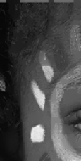
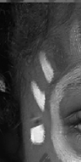
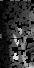
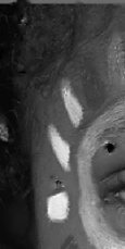
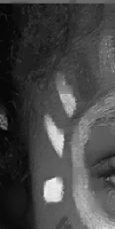
Lost	SKR[5]	CSALSA[7]	CA-FSE bs8
			proposed

Figure 5: Visual reconstruction results for a detail of image 15 of the Kodak database using the dense loss pattern. The lost areas are black in the lower left image.

Acknowledgment

The authors would like to thank Eduard Schön and Nils Genser for their valuable assistance. Further, we gratefully acknowledge that this work has been supported by the Deutsche Forschungsgemeinschaft (DFG) under contract number KA 926/4-2.

References

- [1] C. Fehn, “Depth-Image-Based Rendering (DIBR), Compression, and Transmission for a New Approach on 3D-TV,” San Jose, CA, USA, Jan. 2004, pp. 93–104.
- [2] U. Kim and M. Sunwoo, “New Frame Rate Up-Conversion Algorithms With Low Computational Complexity,” IEEE Trans. on Circuits and Systems for Video Technology, vol. 24, no. 3, pp. 384–393, Mar. 2014.
- [3] N. Bozinovic, J. Konrad, W. Zhao, and C. Vazquez, “On the Importance of Motion Invertibility in MCTF/DWT Video Coding,” in Proc. IEEE Int. Conf. on Acoustics, Speech, and Signal Processing (ICASSP), Philadelphia, PA, USA, Mar. 2005, pp. 49–52.
- [4] W. Schnurrer, J. Seiler, and A. Kaup, “Improving Block-Based Compensated Wavelet Lifting by Reconstructing Unconnected Pixels,” in Proc. IEEE Int. Symposium on Signals, Circuits and Systems (ISSCS), Iasi, Romania, Jul. 2013, pp. 1–4.
- [5] H. Takeda, S. Farsiu, and P. Milanfar, “Kernel Regression for Image Processing and Reconstruction,” IEEE Trans. on Image Processing, vol. 16, no. 2, pp. 349–366, Feb. 2007.
- [6] J. Dahl, P. Hansen, S. Jensen, and T. Jensen, “Algorithms and Software for Total Variation Image Reconstruction via First-order Methods,” Numerical Algorithms, vol. 53, no. 1, pp. 67–92, 2010.
- [7] M. Afonso, J. Bioucas-Dias, and M. Figueiredo, “An Augmented Lagrangian Approach to the Constrained Optimization Formulation of Imaging Inverse Problems,” IEEE Trans. on Image Processing, vol. 20, no. 3, pp. 681–695, Mar. 2011.
- [8] J. Seiler and A. Kaup, “Complex-Valued Frequency Selective Extrapolation for Fast Image and Video Signal Extrapolation,” IEEE Signal Processing Letters, vol. 17, no. 11, pp. 949–952, Nov. 2010.
- [9] ——, “Optimized and Parallelized Processing Order for Improved Frequency Selective Signal Extrapolation,” in Proc. European Signal Processing Conference (EUSIPCO), Barcelona, Spain, Aug. 2011, pp. 269–273.
- [10] N. Asuni and A. Giachetti, “Testimages: A Large-scale Archive for Testing Visual Devices and Basic Image Processing Algorithms,” STAG - Smart Tools & Apps for Graphics Conference, Sep. 2014.
- [11] Kodak test images. http://r0k.us/graphics/kodak/.
- [12] S. Andriani, H. Brendel, T. Seybold, and J. Goldstone, “Beyond the Kodak Image Set: A New Reference Set of Color Image Sequences,” in Proc. IEEE Int. Conf. on Image Processing (ICIP), Melbourne, VIC, Australia, Sep. 2013, pp. 2289–2293.
- [13] D. Scharstein and C. Pal, “Learning Conditional Random Fields for Stereo,” in IEEE Computer Society Conf. on Computer Vision and Pattern Recognition (CVPR), Minneapolis, MN, USA, Jun. 2007, pp. 1–8.
- [14] H. Hirschmüller and D. Scharstein, “Evaluation of Cost Functions for Stereo Matching,” in IEEE Computer Society Conf. on Computer Vision and Pattern Recognition (CVPR), Minneapolis, MN, USA, Jun. 2007, pp. 1–8.
- [15] D. Scharstein, H. Hirschmüller, Y. Kitajima, G. Krathwohl, N. Nešić, X. Wang, and P. Westling, “High-Resolution Stereo Datasets with Subpixel-Accurate Ground Truth,” in German Conf. on Pattern Recognition (GCPR), Münster, Germany, Sep. 2014, pp. 31–42.