PySAGES: flexible, advanced sampling methods accelerated with GPU

Abstract

Molecular simulations are an important tool for research in physics, chemistry, and biology. The capabilities of simulations can be greatly expanded by providing access to advanced sampling methods and techniques that permit calculation of the relevant underlying free energy landscapes. In this sense, software that can be seamlessly adapted to a broad range of complex systems is essential. Building on past efforts to provide open-source community supported software for advanced sampling, we introduce pysages, a Python implementation of the SSAGES that provides full GPU support for massively parallel applications of enhanced sampling methods such as adaptive biasing forces, harmonic bias, or forward flux sampling in the context of molecular dynamics simulations. By providing an intuitive interface that facilitates the management of a system’s configuration, the inclusion of new collective variables, and the implementation of sophisticated free energy-based sampling methods, the pysages library serves as a general platform for the development and implementation of emerging simulation techniques. The capabilities, core features, and computational performance of this new tool are demonstrated with clear and concise examples pertaining to different classes of molecular systems. We anticipate that pysages will provide the scientific community with a robust and easily accessible platform to accelerate simulations, improve sampling, and enable facile estimation of free energies for a wide range of materials and processes.

format/short = ABFshort = abf, long = adaptive biasing force ASEshort = ase, long = Atomic Simulation Environment, first-style = short ANNshort = ann, long = artificial neural networks sampling BCCshort = bcc, long = body-centered cubic CFFshort = cff, long = combined force frequency sampling CVshort = cv, long = collective variable, pdfstring = CV CPUshort = cpu, long = central processing unit, first-style = short, pdfstring = CPU FFSshort = ffs, long = forward flux sampling FUNNshort = funn, long = force-biasing using neural networks JSONshort = json, long = JavaScript Object Notation, first-style = short WTMDshort = wtmd, long = well-tempered metadynamics FESshort = fes, long = free energy surface, short-plural = GAPshort = gap, long = Gaussian Approximation Potential GPUshort = gpu, long = graphics processing unit, first-style = short, pdfstring = GPU TPUshort = tpu, long = tensor processing unit, first-style = short DFTshort = dft, long = density functional theory LDAshort = lda, long = local density approximation, first-style = short MGIshort = mgi, long = materials genome initiative SSAGES short = ssages, long = Software Suite for Advanced General Ensemble Simulations HCGshort = hcg, long = highly coarse-grained HPCshort = hpc, long = high performance computing LCshort = lc, long = liquid crystal LJshort = lj, long = Lennard–Jones MFEPshort = mfep, long = mean free energy pathway MPIshort = mpi, long = message passing interface, first-style = short MDshort = md, long = molecular dynamics MLshort = ml, long = machine learning NNshort = nn, long = neural network GNNshort = gnn, long = Graph neural network DPDshort = dpd, long = dissipative particle dynamics PMEshort = pme, long = particle mesh Ewald RCCshort = rcc, long = Research Computing Center TPSshort = tps, long = time steps per second DOFshort = dof, long = degrees of freedom PLUMEDshort = plumed, long = PLugin for MolEcular Dynamics, first-style = short SMILESshort = smiles, long = simplified molecular-input line-entry system, first-style = short 5CBshort = 5CB, long = 4-cyano-4’-pentylbiphenyl, short-format = SDSshort = sds, long = sodium lauryl sulfate ADPshort = adp, long = alanine dipeptide ns/dayshort = ns/day, long = nano-seconds per day, format =

[pme] organization=Pritzker School of Molecular Engineering, The University of Chicago,addressline=5640 South Ellis Avenue, city=Chicago, state=IL, postcode=60637, country=USA

[rcc] organization=Research Computing Center, The University of Chicago,addressline=6054 S. Drexel Avenue, city=Chicago, state=IL, postcode=60637, country=USA

[ndu] organization=Department of Chemical and Biomolecular Engineering, University of Notre Dame,addressline=250 Nieuwland Hall, city=Notre Dame, state=IN, postcode=46556, country=USA

1 Introduction

Molecular simulations are extensively used in a wide range of science and engineering disciplines [1]. As their use has grown for the discovery of new phenomena and the interpretation of sophisticated experimental measurements, so has the complexity of the systems that are considered. Classical atomistic MD simulations are generally limited to microsecond time scales and length scales of tens of nanometers. For systems that are characterized by rugged free energy landscapes, such time scales can be inadequate to ensure sufficient sampling of the relevant phase space, and advanced methods must therefore be adopted to overcome free energy barriers. In that regard, it is useful and increasingly common to identify properly chosen CV, which are generally differentiable functions of the atomic coordinates of the system; then, biases can be applied to explore the space defined by such CV, thereby overcoming barriers and enhancing sampling of the thermally accessible phase space.

The rapid growth of hardware accelerators such as GPU or TPU, or specialized hardware designed for fast MD computations [2, 3], has provided researchers with increased opportunities to perform longer simulations of larger systems. GPU, in particular, provide a widely accessible option for fast simulations, and several software packages, such as hoomd-blue  [4], Openmm  [5], jax md  [6, 7], LAMMPS  [8], and Gromacs [9], are now available for MD simulations on such devices.

As mentioned above, enhanced sampling methods seek to surmount the high energy barriers that separate multiple metastable states in a system, while facilitating the calculation of relevant thermodynamic quantities as functions of different CV such as FES. Several libraries, such as PLUMED [10], Colvars [11], and our own SSAGES package [12], provide out-of-the-box solutions for performing enhanced sampling MD simulations.

Among the various enhanced sampling methods available in the literature, some of the most recently devised schemes rely on ML strategies to approximate free energy surfaces and their gradients (generalized forces) [13, 14, 15, 16]. Similarly, algorithms for identifying meaningful CV that correlate with high variance or slow DOF are based on deep neural networks [17, 18, 19, 20, 21, 22]. These advances serve to highlight the need for seamless integration of ML frameworks with existing MD software libraries.

To date, there are no solutions that combine enhanced sampling techniques, hardware acceleration, and ML frameworks to facilitate enhanced-sampling MD simulations on GPU. While some MD libraries that support GPU provide access to a limited set of enhanced sampling methods [5, 9, 23, 24, 25], there are currently no packages that enable users to take advantage of all of these features within the same platform and in the same backend-agnostic fashion that tools such as PLUMED and SSAGES have provided for CPU-based MD simulations.

Here we present pysages, a Python Suite for Advanced General Ensemble Simulations. It is a free, open-source software package written in Python and based on jax that follows the design ideas of SSAGES and enables users to easily perform enhanced-sampling MD simulations on CPU, GPU, and TPU. Pysages can currently be coupled with hoomd-blue, Openmm, jax md and ASE   and by extension from the latter to cp2k, Quantum espresso, vasp and Gaussian, among others. At this time, pysages offers the following enhanced sampling methods: Umbrella Sampling, Metadynamics, Well-tempered Metadynamics, Forward Flux Sampling, String Method, Adaptive Biasing Force, Artificial neural network sampling, Adaptive Biasing Force using neural networks, Combined Force Frequency, and Spectral Adaptive Biasing Force. Pysages also includes some of the most commonly used CV and, importantly, defining new ones is relatively simple, as long as they can be expressed in terms of the NumPy [26] interface provided by jax. All CV can be automatically differentiated through jax functional transforms. Pysages is highly modular, thereby allowing for the easy implementation of new methods as they emerge, even as part of a user-facing script.

In the following sections, we provide a general overview of the design and implementation of pysages, and present a series of examples to showcase its flexibility for addressing research problems in different application areas. We also discuss its performance in GPU and present a few perspectives on how to grow and improve the package to cover more research use cases through future development, as well as community involvement and contributions.

2 Implementation

We begin by briefly outlining the core components of pysages, how they function together, and how communication with each backend allows pysages to bias a simulation during runtime. A summary of the execution workflow of pysages along with a mapping of the user interface with the main stages of the simulation and the interaction with the backends, is illustrated in Figure 1.

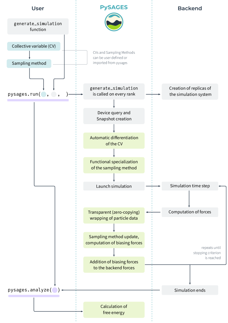
Figure 1: The pysages simulation flowchart. For a simulation, a user sets up a script that declares the CV and sampling methods to be used.

To provide a uniform user interface while minimizing disruption to preexisting workflows, pysages only requires the user to wrap their traditional backend scripting code into simulation generator functions. This approach accommodates the heterogeneity of Python interfaces across the different simulation backends supported by pysages. An example of a simulation generator function and how a traditional Openmm script can be modified to perform an enhanced-sampling MD simulation is depicted in Figure 2.

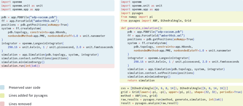
Figure 2: Example of how to use the Python interface for pysages. It is easy to extend existing MD scripts with pysages to perform enhanced-sampling MD, with minimal changes to the code. In general, the only requirement is for the user to wrap the code that defines the simulation system into a simulation generator function.

At the start of a simulation, the simulation generator function is called to instantiate as many replicas of the simulation as needed. Then, for each replica, pysages queries the particle information and the device that the backend will be using. In addition, during this initial stage pysages also performs automatic differentiation of the collective variables via jax’s grad transform   required to estimate the biasing forces, and generates specialized initialization and updating routines for the user-declared sampling method.

Like SSAGES, pysages wraps the simulation information into an object called a Snapshot. This object exposes the most important simulation information, such as particle positions, velocities, and forces in a backend- and device-agnostic format. To achieve this, pysages uses dlpack  [27]   for c++ based MD libraries   to directly access the contents of the backend-allocated buffers for the different particle properties without creating data copies whenever possible.

Once the setup of both the simulation and sampling method is completed, pysages hands control back to the backend, which will run for a given number of time steps or until some other stopping criteria is reached. In order to exchange information back and forth, pysages adds a force-like object or function to the backend which gets called as part of the time integration routine. Here, the sampling method state gets updated and the computed biasing forces are added to the backend net forces.

Finally, the information collected by the sampling method is returned and can be used for calculating the free energy as function of the selected CV. Unlike SSAGES, pysages offers a user-friendly analyze interface that simplifies the process of performing post simulation analysis, including the automatic calculation of free energies based the chosen sampling method. This feature can greatly reduce the time and effort required to gain valuable insights from simulations.

Pysages offers an easy way to leverage different parallelism frameworks including MPI with the same uniform fronted available to run enhanced sampling simulations. This is achieved via Python’s concurrent.futures interface. In particular, for MPI parallelism, the user only needs to pass an additional MPIPoolExecutor (from mpi4py) to pysages’ run method. If the user selects a method such as UmbrellaSampling, the workload for each image will be distributed across available MPI nodes. On the other hand, for most of the sampling methods, the parallelization interface allows the user to run multiple replicas of the same system to enable, for instance, analysis of the uncertainties associated to computing the free energy of a given system.

To ensure the reproducibility and correctness of our implementation and to follow software engineering best practices, we have implemented a comprehensive unit tests suite, and leverage GitHub’s continuous integration services. In addition, we use trunk.io [28] to adhere to quality standards as well as to ease the collaboration of developers.

2.1 Enhanced Sampling Methods

While we assume the reader has some basic understanding of enhanced sampling methods, here we provide an overview of these techniques. We direct readers interested in learning more about the fundamentals of enhanced sampling to a number of excellent recent review articles [29, 30, 31, 32, 33, 34, 35, 36, 37, 38]. In addition, we discuss the general structure of how enhanced sampling methods are implemented within pysages, and also present a summary of the various methods already available in the library.

Enhanced sampling methods are a class of simulation techniques that manipulate regular MD simulations in order to more effectively sample the configuration space. In MD a CV, $\xi$, is typically a function of the positions of all particles, $\hat{\xi}(\{r_{i}\})$.

For a given statistical ensemble (such as the canonical, nvt), the corresponding free energy can be written as $A=-k_{\text{B}}T\ln(Z)$, where $A$ is the Helmholtz free energy and $Z$ is the canonical partition function. To make explicit the dependency of the free energy on $\xi$, let us write down the partition function:

$$Z(\xi)\propto\int\text{d}^{N}r_{i}\;\delta(\hat{\xi}(\{r_{i}\})-\xi)\;e^{-U(\{r_{i}\})/k_{\text{B}}T}$$ (1)

Normalizing this partition function gives us the probability of occurrence, $p(\xi)=Z(\xi)/(\int\text{d}\xi\;Z(\xi))$, for configurations in the CV subspace. Substituting this probability into the expression for the free energy, we get:

$$A(\xi)=-k_{\text{B}}T\ln(p(\xi))+C$$ (2)

where $C$ is a constant.

If we take the derivative of the free energy with respect to $\xi$ we get

$$\frac{dA(\xi)}{d\xi}=\frac{\int\text{d}^{N}r_{i}\;\frac{dU}{d\xi}\;\delta(\hat{\xi}(\{r_{i}\})-\xi)\;e^{-U(\{r_{i}\})/k_{\mathrm{B}}T}}{\int\text{d}^{N}r_{i}\;\delta(\hat{\xi}(\{r_{i}\})-\xi)\;e^{-U(\{r_{i}\})/k_{\mathrm{B}}T}}=\bigg{\langle}\frac{dU}{d\xi}\bigg{\rangle}_{\!\!\xi},$$ (3)

where $\langle\ldots\rangle_{\xi}$ denotes the conditional average.

The goal of CV-based enhanced sampling methods is to accurately determine either $p(\xi)$ or $dA(\xi)/d\xi$   from which $A(\xi)$ can be recovered   in a computationally tractable manner.

In pysages, the implementation of sampling methods follows the jax functional style programming model. New methods are implemented as subclasses of the SamplingMethod class, and are required to define a build method. This method returns two methods, initialize and update, used as part of the process of biasing the simulation. For readers familiar with jax md, these could be thought of as analogues to the higher level functions returned by jax md’s simulate integration methods. The initialize method allocates all the necessary helper objects and stores them in a State data structure, while the update method uses the information from the simulation at any given time to update the State.

While pysages allows new methods to be written seamlessly as part of Python scripts used to set up molecular dynamics simulations, it also provides out-of-the-box implementations of several of the most important known sampling methods. We list and briefly detail them next.

2.1.1 Harmonic Biasing

One simple way to sample a specific region of the phase space is to bias the simulation around a point $\xi_{0}$ with harmonic bias. This adds a quadratic potential energy term to the Hamiltonian that increases the potential energy as a system moves away from the target point: $\mathcal{H}_{b}=\mathcal{H}+k/2(\xi-\xi_{0})^{2}$, where $k>0$ is the spring constant. The unbiased probability distribution $p(\xi)$ can be recovered by dividing the biased distribution by the known weight of the bias $p(\xi)=p_{b}(\xi)/e^{-k/2(\xi-\xi_{0})^{2}/k_{\text{B}}T}$.

The disadvantage of this approach is that it can only be used to explore the free energy landscape near a well-know point in phase space. This may not be sufficient for many systems, where the free energy landscape is complex.

2.1.2 Umbrella Sampling

Umbrella sampling is a technique that traditionally builds on harmonic biasing by combining multiple harmonically-biased simulations. It is a well-known method for exploring a known path in phase space to obtain a free energy profile along that path [39, 40]. Typically, a path between to point of interest is described by $N$ points in phase space, $\xi_{i}$. At each of these points, a harmonically biased simulation is performed, and the resulting occurrence histograms are combined to obtain a single free energy profile.

In pysages, we implement umbrella integration for multi-dimensional CV. This method approximates the forces acting on the biasing points and integrates these forces to find the free energy profile $A(\xi)$, and allows to explore complex high-dimensional free energy landscapes.

2.1.3 Improved String Method

When only the endpoints are known, but not the path itself, the improved (spline-based) string method can be used to find the MFEP between these two endpoints [41]. The spline-based string method improves upon the original string method by interpolating the MFEP using cubic-splines. In this method, the intermediate points of the path are moved according to the recorded mean forces acting on them, but only in the direction perpendicular to the contour of the path. This ensures that distances between the points along the path remain constant.

This method has been widely used and has been shown to be an effective way to find the MFEP between two points in the phase space [41].

2.1.4 Adaptive Biasing Force sampling

The ABF sampling method is a technique used to map complex free-energy landscapes. It can be applied without prior knowledge of the potential energy of the system, as it generates on-the-fly estimates of the derivative of the free energy at each point along the integration pathway. ABF works by introducing an additional force to the system that biases the motion of the atoms, with the strength and direction of the bias continuously updated during the simulation. In the long-time limit, this yields a Hamiltonian with no average force acting along the transition coordinate of interest, resulting in a flat free-energy surface and allowing the system to display accelerated dynamics, thus providing reliable free-energy estimates [42, 43]. Similarly to SSAGES, pysages implementation of ABF is based on the algorithm described in [43].

2.1.5 Metadynamics

Metadynamics is another popular approach for enhancing sampling of complex systems. In metadynamics [44], a bias potential is applied along one or more CV in the form of Gaussian functions. The height and width ($\sigma$) of these Gaussians are controlled by the user. The Gaussian bias potentials are cumulatively deposited at user-defined intervals during the simulation. In standard metadynamics, the height of the Gaussian bias potentials is fixed.

In contrast, for WTMD [45] simulations, the height of the Gaussian bias potentials is adjusted at each timestep using a preset temperature based bias factor. This scaling of Gaussian heights in WTMD leads to faster convergence compared to standard metadynamics, as it restricts the range of free energy explored to a range defined by the bias factor.

In pysages, we have implemented both standard metadynamics and WTMD. The well-tempered variant is activated when a user sets a value for the bias factor. To improve the computational performance, we have added optional support for storing the bias potentials in both on a pre-defined grid. This allows users to trade-off accuracy for faster simulations, depending on their needs.

2.1.6 Forward Flux Sampling

FFS belongs to a different family of enhanced sampling methods than the ones described above. In the previously described methods, the free energy change from a region in the phase space ($A$) to the region of interest ($B$) is calculated by applying a bias to the system. In FFS no bias is added and instead an efficient selection of trajectories that crosses the phase space from $A$ to $B$ is performed. Since no bias is used, the intrinsic dynamics of the system is conserved and therefore kinetic and microscopic information of the transition path can be studied [46]. In pysages we have implemented the direct version of FFS [47, 48].

2.1.7 Artificial neural networks sampling

ANN [13] employs regularized neural networks to directly approximate the free energy from the histogram of visits to each region of the CV space, and generates a biasing force that avoids ringing and boundary artifacts [13], which are commonly observed in methods such as metadynamics or basis functions sampling [49]. This approach is effective at quickly adapting to diverse free energy landscapes by interpolating undersampled regions and extrapolating bias into new, unexplored areas.

The implementation on pysages offers more flexible approaches to network regularization than SSAGES, which uses Bayesian regularization.

2.1.8 Force-biasing using neural networks

FUNN [14] is based upon the same idea as ANN, that is, relying on artificial neural networks to provide continuous functions to bias a simulation, but instead of using the histogram to visits to CV space it updates its network parameters by training on the ABF estimates for the mean forces as the simulation advances. This method shares all of the features of ABF, but the smooth approximation of the generalized mean force it produces enables much faster convergence to the free energy of a system compared to ABF.

2.1.9 Combined Force Frequency sampling

The CFF method [15] combines the speed of generalized-force based techniques such as ABF or FUNN with the advantages of frequency-based methods like metadynamics or ANN. Notable improvements over earlier force-based methods include eliminating the need for hyperparameters to dampen early-time estimates, automating the integration of forces to generate the free energy, and providing an explicit expression for the free energy at all times, enabling the use of replica exchange or reweighing.

In principle, by using sparse storage of histograms, it should be possible to scale the method to higher dimensions without encountering memory limitations, such optimization is however not yet implemented in pysages.

2.1.10 Spectral Adaptive Biasing Force

Spectral ABF [50] is a method that follows the same principle as neural-network-based sampling methods, in that it builds a continuous approximation to the free energy. However, in contrast to methods like FUNN it does so by fitting exponentially convergent basis functions expansions, and could be thought as a generalization of the Basis Functions Sampling Method. In contrast to the latter, and similar to CFF, it allows for the recovery of an explicit expression for the free energy of a system. It is an extremely fast method in terms of both runtime and convergence.

2.2 Collective variables

As previously mentioned, enhanced sampling calculations commonly involve the selection of a CV. An appropriate CV for a given system could simply be the distance between the centers of mass of two groups of atoms, but could be a complex specialized quantity.

Below, we list a set of CV predefined in pysages, sorted by the number of groups of atom coordinates necessary for their use:

1. TwoPointCV. This subclass is for CV that need two groups for their definition. This includes Distance and Displacement (vector).

2. ThreePointCV. Subclass of CV with three groups of atoms, such as Angle.

3. FourPointCV. Subclass of CV with four groups of atoms, such as DihedralAngle.

4. AxisCV. Subclass of CV that are projected on a determinate axis. This includes Component and PrincipalMoment.

5. CollectiveVariable General base class for all CV. In pysages, CV that directly derive from this class, and do not belong to the previous groups, include: RingPhaseAngle, RingAmplitude, RadiusofGyration, Asphericity, Acylindricity, ShapeAnisotropy, RingPuckeringCoordinates [51] (vector).

In pysages we provide users with a simple framework for defining CV, which are automatically differentiated with jax. To illustrate this, we compare how to write the calculation of a CV that measures the projection of the vector between two groups of atoms over the axis that passes by other two groups, in both SSAGES and pysages (see Figure 3). In pysages the gradient calculation is done automatically whereas in SSAGES it has to be coded explicitly.

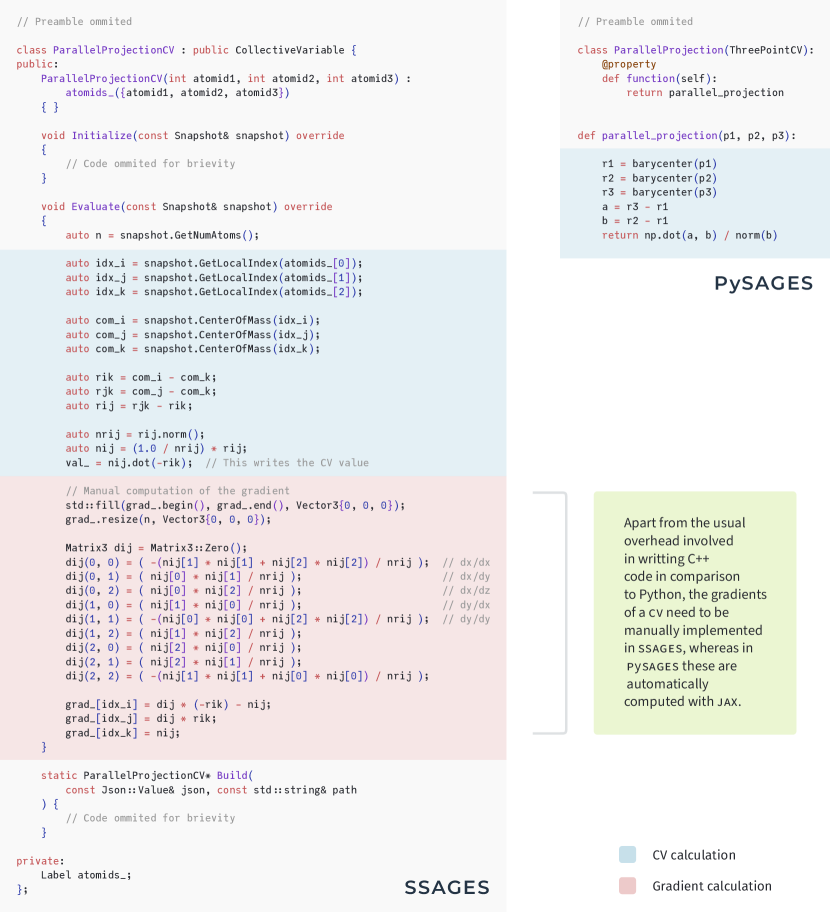
Figure 3: Example of how to write a CV in pysages. On the left is the same CV written in SSAGES and on the right the pysages version. In general, the only requirement is for the user to write the CV as a differentiable function in jax.

Data-driven and differentiable CV discovered using artificial neural networks (e.g. autoencoders) [29, 21, 18, 52, 53] with arbitrary featurizations of atoms can in principle be implemented in pysages based on the above general abstract classes of CV.

The following second example shows the power of differential programming for CV declaration in pysages.

2.2.1 Case study: A CV for interfaces

When the two immiscible liquids are in contact with each other, the density of one liquid experiences a gradual change. This transition region is the liquid-liquid interface and its position has high importance in many studies (see section 3.1.3). However, the location of such interface is not a trivial task since it generally fluctuates as the simulation progresses. As a representative CV for the interface, we can utilize the position of the point where the gradient of the density is maximized. More formally, let $\rho(x)$ denote the density of a liquid of interest at a coordinate $x$ on the perpendicular axis. We would like to find the location of the interface:

$$I=\arg\max_{x}|\rho^{\prime}(x)|$$ (4)

However, the density function $\rho(x)$ is not directly measurable in a molecular simulation, as the coordinates of atoms are discrete. To obtain an approximation of $\rho(x)$, we divide the coordinates into multiple bins, each with a width of $\delta$, and create a histogram $p(x)$ that records the number of atoms falling into the bin around position $x$. In other words,

$$p(x)=\sum_{i=1\ldots n}\big{[}\,|x_{i}-x|<\delta/2\,\big{]}$$ (5)

in which $x_{i}$ denotes the coordinate of atom $i$. As written above, $p(x)$ is non-differentiable. Therefore, as in other works [54], we utilize the kernel density trick with a Gaussian kernel to modify $p(x)$. The modified $\tilde{p}(x)$, is defined as:

$$\tilde{p}(x)=\sum_{i=1\ldots n}\exp{\left(-\frac{(x_{i}-x)^{2}}{2\sigma^{2}}\right)}$$ (6)

in which $\sigma$ is a hyperparameter that decides the width of the Gaussian kernel. Then, the gradient of the density can be approximated as:

$$\tilde{p}\,^{\prime}(x)=\frac{\tilde{p}(x+\delta/2)-\tilde{p}(x-\delta/2)}{\delta}$$ (7)

and we calculate the location of the interface as $I=\arg\max_{x}|\tilde{p}\,^{\prime}(x)|$. The $\arg\max$ operator is also non-differentiable. As a result, we replace it with a softmax function that transforms the raw input into a probability. Denote the $m$ bins as $j=1\ldots m$, and finally we calculate the location of the interface as:

$$I=\frac{\sum_{j}x_{j}\,\exp|\tilde{p}\,^{\prime}(x_{j})|}{\sum_{j}\exp|\tilde{p}\,^{\prime}(x_{j})|}$$ (8)

As demonstrated in the code snippet for this CV, provided in A, pysages allows for the concise and straightforward implementation of complex CV such as this one.

3 Results and Discussion

To evaluate a software package like pysages, we must consider at least two factors: physical correctness and computational performance.

First, to assess the correctness of the enhanced sampling methods implemented in pysages, we present in B.1 the free-energy landscape for the dihedral angles $\phi$ and $\psi$ of ADP. This example is commonly used to benchmark new enhanced sampling algorithms. Similarly, we also show in B.2 the free-energy as a function of the dihedral angle of butane. Our results show that pysages reproduces the expected free-energy landscapes using different methods and backends. In section 3.1, we further investigate the applicability and correctness of pysages beyond these simple model systems.

Second, we demonstrate the performance of pysages on GPU with two different backends in section 3.2. In particular, we compare the performance of enhanced sampling simulations to the performance of pure MD simulations, as well as other enhanced sampling implementations.

3.1 Example applications of enhanced sampling with pysages

To demonstrate the versatility and effectiveness of pysages in different contexts, we present several examples of how enhanced sampling methods can be used to gain valuable insights in various fields including biology, drug design, materials engineering, polymer physics, and ab-initio simulations. These examples showcase how pysages can be used in diverse research areas and the utility of different enhanced sampling methods and backends.

Overall, these examples confirm that the enhanced sampling methods implemented in pysages work as intended and provide results consistent with existing literature.

3.1.1 Structural Stability of Protein–Ligand Complexes for Drug Discovery

High-throughput docking techniques are a widely-used computational technique in drug lead discovery. However, these techniques are limited by the lack of information about protein conformations and the stability of ligands in the docked region [55]. To address this issue, the Dynamical Undocking (duck) method was developed to evaluate the stability of the ligand binding by calculating the work required to break the most important native contact (hydrogen bond interactions) in the protein-ligand complex [56]. This method has been shown to be complementary and orthogonal to classical docking, making both techniques work parallel in drug discovering [57, 58]. However, duck can be slow to converge when combined with traditional enhanced sampling techniques [56], making it unsuitable for high-throughput drug discovery protocols.

Here, we demonstrate how pysages with Openmm can be used efficiently in drug discovery applications, where the user-friendly interface, native parallel capabilities, and new enhanced sampling methods with fast convergence are synergistically combined to accelerate the virtual screening of ligand databases. In this example, we study the main protease (Mpro) of Sars-CoV-2 virus (pdb: 7ju7 [59]), where the ligands were removed and the monomer A was selected as the docking receptor. A ligand with SMILES string CCCCOCC(=O)c1ccc(C)cc1N[C@H]1N[C@@H](c2cccnc2)CS1 was docked using RDock [60]. The best scoring pose was used to initialize the system, which was simulated using the ff14sb [61], tip3p [62], and gaff [63] force fields. A 10 ns equilibration procedure was carried out to find the most stable hydrogen bond between the ligand and the protein. The last frame of this equilibration was then used to initialize the enhanced sampling calculations in pysages with ABF, metadynamics, FUNN, ANN, and Spectral ABF. These methods were compared against the same system simulated using Amber20 [64] with Steered Molecular Dynamics (see Figure 4b). Our results suggest that we can reduce the simulation time by an order of magnitude using new enhanced sampling methods like Spectral ABF or FUNN. This can greatly accelerate the drug discovery process and help identify potential drug leads more quickly.

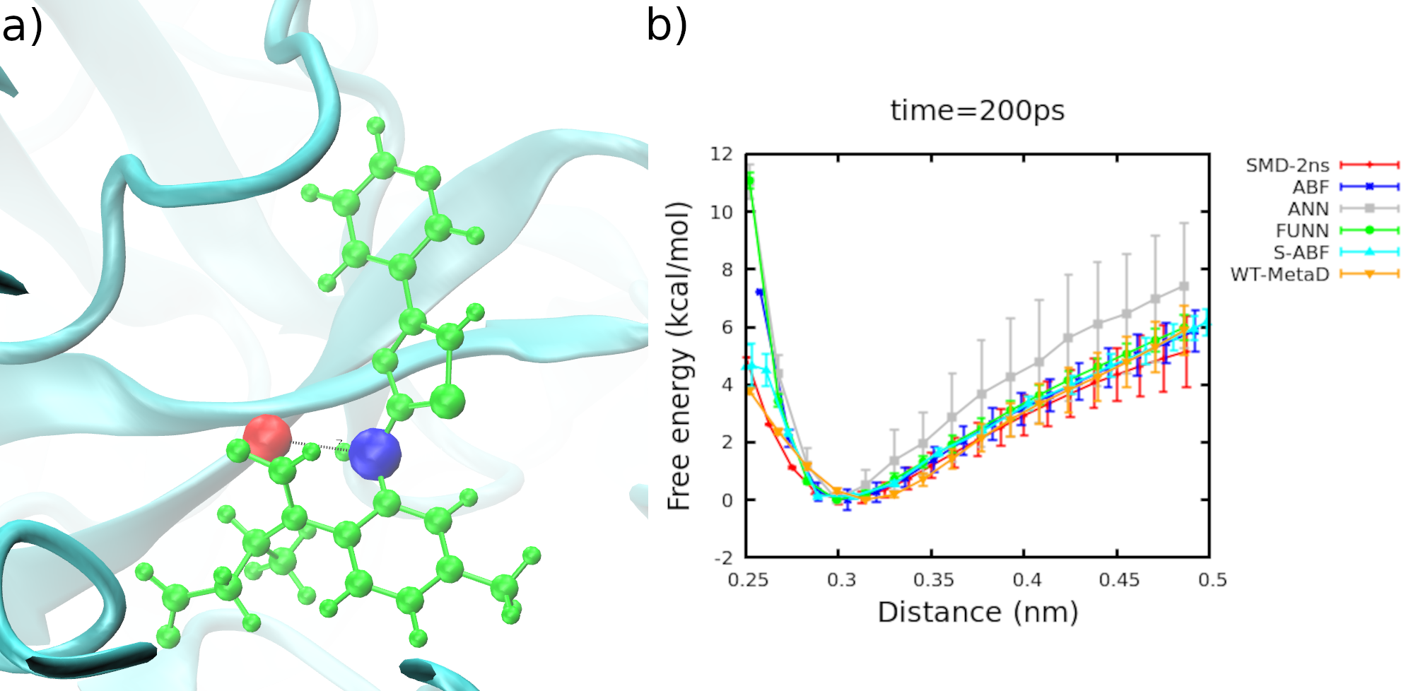
Figure 4: Dynamical Undocking (duck) method in detail. For a proposed binding mode obtained from classical docking, a short run using MD simulations is carried out and the most stable receptor-ligand native contact is selected from that run. In this case, it is the hydrogen bond between the red and blue atoms highlighted in panel a). b) Comparison between different methods in pysages for duck calculations averaged over 5 different replicas for each method. The reference, a Steered MD simulations simulations of 2 ns is in red. In comparison, different methods in pysages are used considering simulation period 10 times shorter: only ANN [13] provides inferior performance against the reference; Spectral ABF [50] or FUNN [14] give the best performance.

3.1.2 Fission of a Diblock Copolymer Spherical Domain

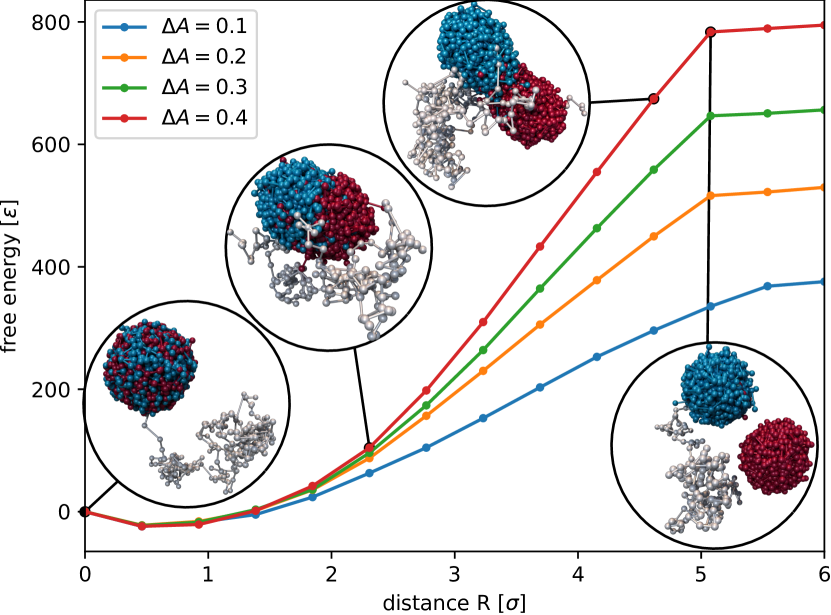
Figure 5: Free energy landscape of the fission of a spherical diblock-copolymer domain. The chain ends forming the spherical domain are split into two groups (blue) and (red), the other chain ends not visible for clarity except for a single chain (grey). Initially, a single spherical domain is formed, but as we constraint the center of mass between the blue and red groups further, the domain first elongates and then separates completely. During this separation, the free energy continuously increases and the increase is steeper for high repulsion between unlike type $\Delta A$. As soon as the domain is separated, the free energy plateaus.

We now investigate the fission of a single spherical domain of a diblock copolymer using a coarse-grained model. We use a soft, coarse-grained DPD model published in previous studies [65, 66, 67]. The model consists of $n=200$ chains with $N=256$ beads each, representing a liquid polymer melt. The first $N_{A}=16$ beads in each chain are type A, while the remaining $N_{B}=240$ are type B.

A standard DPD potential is used to enforce incompressibility with a repulsion parameter of $A_{ii}=5k_{B}T/\sigma^{2}$. However, a higher interaction of $A_{AB}=A_{ii}+\Delta Ak_{B}T/\sigma^{2}$, with $\Delta A\in[0.1,0.4]$ is applied between unlike particles to create a repulsion that leads to a microphase separation. A Flory-Huggins parameter $\Delta A\propto\chi N>0$ can characterize this phase separation. The interaction range of this non-bonded potential is $1\sigma$, as well as the range of the DPD thermostat that keeps the temperature at $T=1k_{B}T=1\epsilon$.

In addition, a harmonic spring force with zero resting length is used to connect the beads to polymer chains with a spring constant of $k=16/3k_{B}/\sigma^{2}$, resulting in an average bond length of $b_{0}=0.75\sigma$. The equilibrium phase for this polymer melt is a BCC phase of spherical A droplets inside a B melt. [68] However, we confine the polymer to a tight cubic simulation box of length $L_{0}=10\sigma$, which results in a single A spherical domain in the B matrix. We integrate the simulation with a time step of $\Delta t=10^{-3}\tau$ and each simulation is equilibrated for $t=1000\tau$, followed by a production run of $t=1000\tau$ as well. A discussion of the GPU performance of this system with and without pysages can be found in section 3.2.1.

After defining the diblock copolymer system, the next step is to define a CV within the system. In this case, we are interested in the fission of the single spherical A domain into two equally sized smaller A domains. To achieve this, we divide the polymer chains into two groups: the first $n=100$ chains are going to form the first small domain (blue in Figure 5) and the second $n=100$ chains form the second spherical domain (red in Figure 5). To define and enforce the separation of the two groups, we define our CV as the distance, $R$, between the center of mass of the blue A-tails and the center of mass of the red A-tails. Initially, without biasing, the two groups form a single spherical domain and blue and red polymer tails are well mixed, as shown at small $R<1\sigma$ in Figure 5.

To study the separation of the spherical domain, we use harmonic biasing (see section 2.1.1) to enforce a separation distance $R_{0}$ between the two groups. The high density in the system $\sqrt{\text{{$\bar{\mathcal{N}}$}}}=\frac{\rho_{0}}{N}R_{e0}^{3}\approx 344$, leads to low fluctuations and suppression of unfavorable conformations. Therefore, we use a high spring force constant of $k_{CV}=1500\epsilon/\sigma^{2}$ to facilitate the separation.

We investigate a separation of $R\in[0,6]\sigma$ with 14 replicas and use umbrella integration (see section 2.1.2) to determine the free energy profile, as shown in Figure 5. As we increase the external separation distance $R_{0}$, we observe how the single domain splits into two. At a low separation distance $R<2\sigma$, the single domain is mostly undeformed, but the two groups separate inside the single spherical domain. Increasing the separation distance further goes beyond the dimensions of the spherical domain, leading to the deformation of the domain into an elongated rod-like shape. The two groups still maintain a connection to minimize the AB interface.

At a separation between $4\sigma$ and $5\sigma$ the deformation becomes so strong, that the penalty of forming another AB interface between the two groups, and hence forming two spherical domains, is lower than the entropic penalty of the domain deformation and elongated AB interface of the droplet. After the separation, the free energy landscape remains indifferent to the separation, since there is no interaction between the two domains left.

The free energy profile of separation is controlled by the repulsion of unlike types $\chi N\propto\Delta A$. The stronger the repulsion, the more energy is necessary to enlarge the AB surface area for the fission. For the strongest interaction $\Delta A=0.4\epsilon$, the total free energy barrier reaches about $800\epsilon$, while for the lowest $\Delta A=0.1\epsilon$ it remains below $400\epsilon$. Both barriers are orders of magnitude larger than thermal fluctuations $1k_{B}T=1\epsilon$, so a spontaneous separation is not expected and the fission can only be studied via enhanced sampling.

It is interesting to note that at the lowest separation distance $R_{0}=0$ it is not the lowest free energy state. Enforcing perfect mixing is not favorable, as the two groups naturally want to separate slightly optimizing the entropy of the chain end-tails.

3.1.3 Liquid Crystal Anchoring in Aqueous Interfaces

LC, materials that flow like liquids but have anisotropic properties as crystals, have been used lately as prototypes for molecular sensors at interfaces given the high sensitivity in their anchoring behavior relative to small concentration of molecules at aqueous interfaces [69]. The presence of molecules at the interface changes drastically the free energy surface of LC molecules relative to their orientation and distance to such interface. In this example, we are revisiting some canonical interfaces for LC; 5CB at the interface of pure water and SDS. For 5CB and water, previous work has focused on obtaining the free energy surface of a 5CB at the water interface [70]. In our case, hybrid anchoring conditions have been imposed on a 16 nm slab of 1000 5CB molecules in the nematic phase (300 K) interacting with a 3 nm slab of water with 62 molecules of SDS at one of the interfaces. The force fields used are: united atom for 5CB [71], tip3p [62] for water, gaff [63] and Lipid 17 for SDS. The CV chosen to study this system are the distance of the center of mass of one molecule of 5CB at each one of the interfaces (see A), and the tilt orientation of the same molecule with respect to the z axis of the box. The free energy surfaces for the pure water and with SDS at the interface are both displayed in Figure 6. We can observe that the free energy surface of pure water shows a minimum corresponding to a parallel orientation to the surface with a similar shape that one calculated in [70]. On the contrary, the presence of SDS transforms the minimum to a maximum in the same relative position and orientation to the interface (Figure 6 top left), moving now the minima to a perpendicular orientation of 5CB to the interface, in agreement to the experimental observation of change from planar to homeotropic anchoring in the presence of SDS in water.

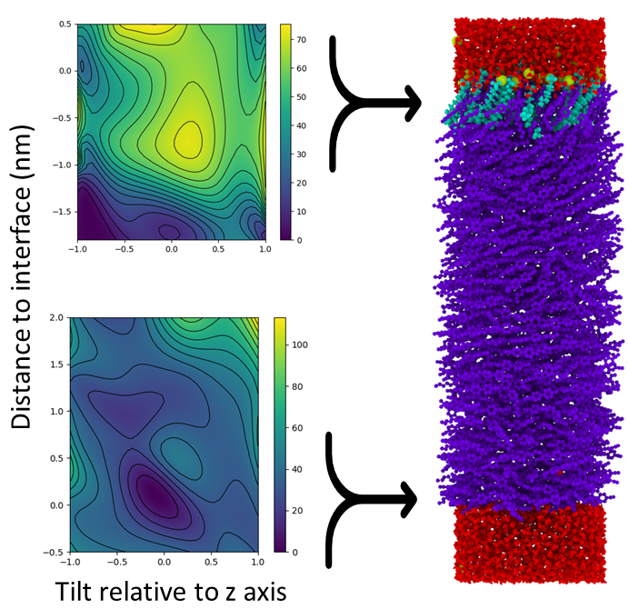
Figure 6: Free energy surface of 5CB in a hybrid anchoring slab with SDS and water. Right: Snapshot of the system with water molecules in red, 5CB in purple, SDS in green and sodium ions in yellow. Top Left: FES of 5CB molecule near the water–SDS interface. Bottom Left: FES of 5CB near a pure water interface. Both FES were obtained with pysages and Openmm using the FUNN method.

3.1.4 Ab Initio Enhanced Sampling Simulations

In the field of ab initio simulations of heterogeneous catalysis, capturing the dynamic and entropic effects is crucial for an accurate description of the phenomena [38]. Classical force fields are inadequate for capturing the essential bond breaking events involved in catalysis, so MD simulations based on first-principles calculations are necessary. Given that reactive events are often limited by large free energy barriers, enhanced sampling techniques are a crucial part of these simulations. Coupling pysages to ASE, provides access to a wide range of first-principle calculators.

As an example, we have used vasp as a calculator for a simple ab initio enhanced sampling simulation. The CV is the separation distance between a sodium and chlorine atom using the pbe functional [72], and Spectral ABF as the enhanced sampling method (see section 2.1.10). The results are shown in Figure 7, where the minimum in the free energy profile along the Na–Cl distance corresponds to the equilibrium distance between Na and Cl atoms in vacuum.

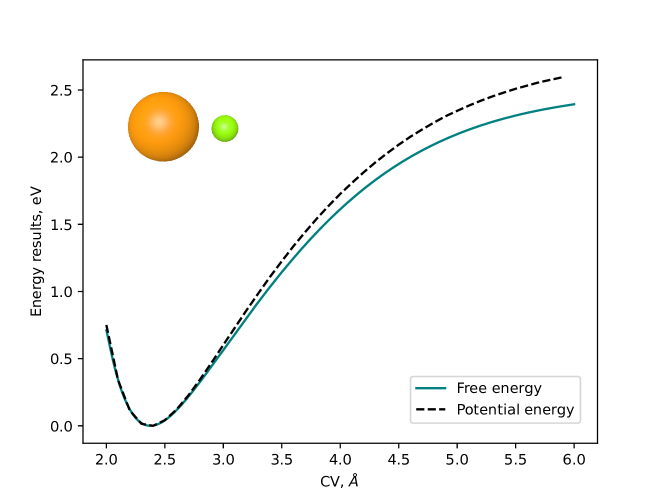
Figure 7: Free energy ($T=300$ K) and potential energy calculations of Na–Cl distance with ASE + vasp using Spectral ABF in pysages.

3.1.5 Enhanced Sampling with Machine Learning Force Fields

Deep NN force fields can retain the accuracy of ab initio MD while allowing for computational costs similar to those of classical MD. Through ASE it is possible to access NN potentials such as Deepmd  [73], and the GAP. Additionally, jax md allows to leverage more general NN potentials that can be used in enhanced sampling calculations. Coupling of pysages with ASE or jax md can be used in active learning of NN force fields by efficiently sampling rare events using any of the enhanced sampling methods provided by pysages as described in Ref. [74] where parallel tempering metadynamics was used to generate accurate NN force field in urea decomposition in water.

To test the capabilities of pysages to handle different NN force fields, we have selected three different systems trained with the methods mentioned above. For Deepmd, we use a pre-trained model for water, where the enhanced sampling system is one single water molecule in vacuum, the collective variable is the internal angle of the molecule and the sampling method is ABF (section 2.1.4). The results in Figure 8 show that the minimum for this free energy profile is around 105 degrees, which is within the range of the experimental value.

Next, in Figure 8b, a GAP potential was used for Si–H amorphous mixtures [75]. In this case, a system of 244 atoms was used, and the collective variable is the bond angle between a triad of Si–Si–H atoms in the mixture. The global minimum in free energy agrees with the histogram taken from unbiased simulations reported in [75].

Lastly, we studied a GNN model of a Si crystal [76] with pysages and jax md. In this case, a crystalline Si system of 64 atoms was used, and the CV was the Si–Si distance for the the crystal. The results of Figure 8c show that for this model, the minimum in the free energy corresponds almost exactly to the experimental value for the Si–Si nearest distance of 2.35 Å.

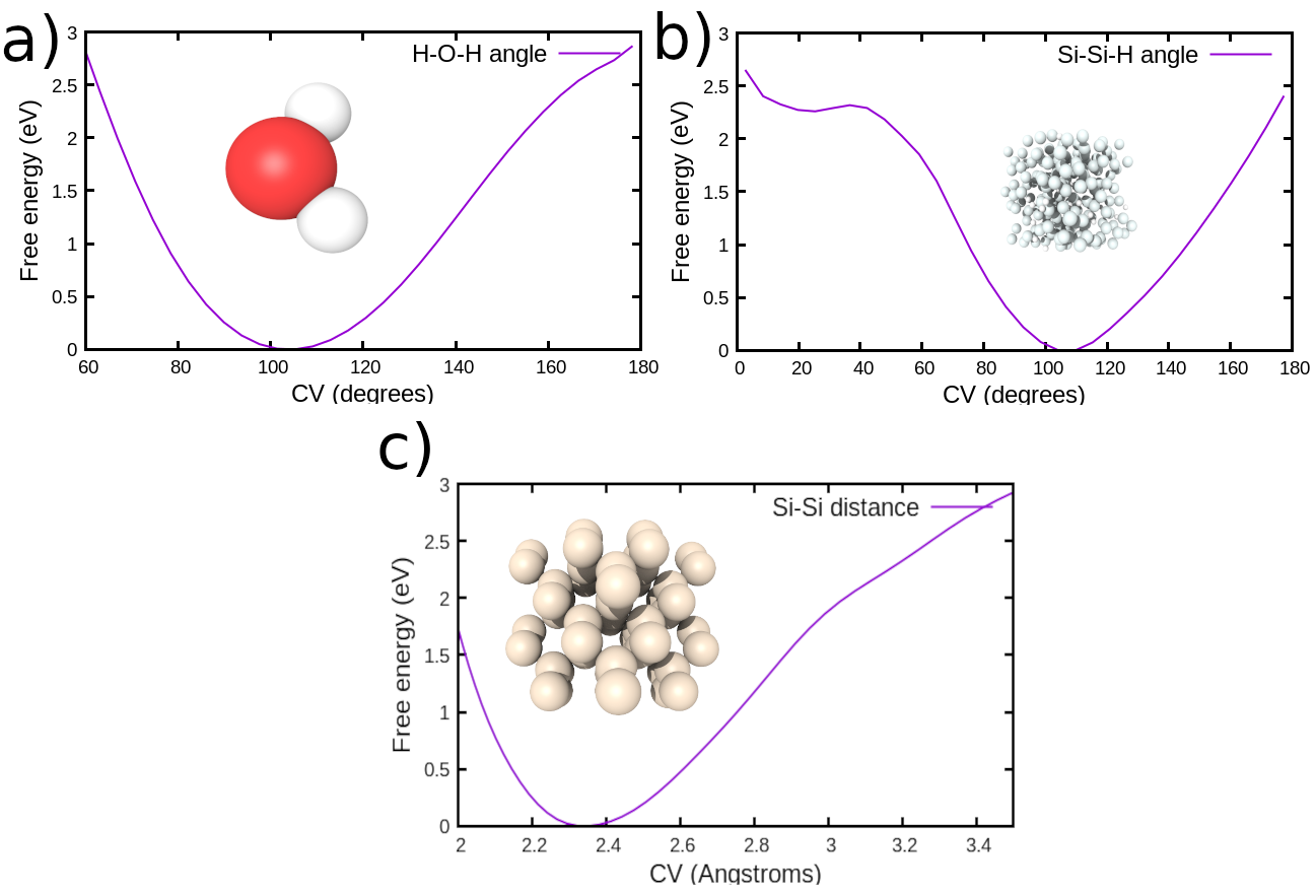
Figure 8: Free energy calculation of: a) Water internal angle from a Deepmd model with ASE, b) Si–Si–H angle of GAP model with ASE and c) Si–Si distance of a GNN model with jax md.

3.2 Performance

Our analysis revealed that pysages is at least $\sim$14–15 times faster than SSAGES on an Nvidia v100 GPU machine. To obtain this estimate, we ran enhanced sampling using umbrella sampling along the center of mass distance between two spherical polymer domains to measure the free energy landscape of the fission of a spherical diblock-copolymer blend (Figure 5) described in section 3.1.2. For support and compatibility across libraries and MD engine versions, we estimated the performance with SSAGES v0.9.2-alpha and pysages v0.3.0 using hoomd-blue v2.6.0 and hoomd-blue v2.9.7, respectively.

3.2.1 GPU utilization analysis

Pysages is designed to execute every compute-intensive step of a simulation on the GPU and have zero copy instruction between GPU device and host CPU memory for its explicit backends for hoomd-blue  [4] and Openmm  [5], while still providing Python code for the user through jax  [77]. In this section, we investigate the calculation efficiency of pysages by examining two example systems, one for each backend.

For hoomd-blue, we are investigating a system of highly coarse-grained DPD diblock-copolymers as discussed in section 3.1.2. The simulation box contains a total of $nN=51\,200$ particles at a density of $\rho=51.2/\sigma^{3}$, which we use for benchmarking purposes with an Nvidia v100 GPU hosted on an Intel Xeon Gold 6248r CPU @ 3.00GHz. Running only with hoomd-blue v2.9.7 we achieve an average TPS of $754$, which is the expected high performance of hoomd-blue on GPU.

Figure 9 shows a detailed profiled timeline during the execution of a single time step. During $1.8$ ms, hoomd-blue spends the most computational effort on the calculation of pairwise DPD forces. It can be noted that hoomd-blue is designed to have almost no idle time of the GPU during a time step. As soon as pysages is added computation part, we observe that an additional part is added to calculate the CV and add the forces to every particle. This causes a small period of idle of the GPU, since the execution also requires action of the Python runtime interface with jax.

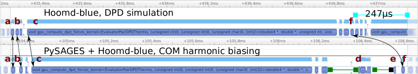
Figure 9: The figure shows a $1.8$ms section of profiled timeline recorded with Nvidia Nsight systems on an Nvidia v100 GPU. The top row shows a vanilla hoomd-blue simulation step, while the bottom row shows a pysages/hoomd-blue simulation with harmonic biasing of a center of mass CV. Light-blue represents the GPU activity while dark-blue represents individual cuda compute kernels. The maroon letters show case the same compute steps in both simulations: a) First half-step of integration, b) compute of bond forces, c) pair-forces, d) calculation of the CV, e) addition of the harmonic biasing force to the hoomd-blue simulation, and f) the second integration step. Sections d) and e) are pysages only and are executed on the GPU. We observe GPU idle time during the pysages Python coordination with GPU–jax/cupy (green bar), but note that there is no memory copies even within the GPU memory. The additional time for CV biasing per time step is $247\leavevmode\nobreak\ \upmu$s (teal bar).

In the future, we plan to launch the calculation of CV asynchronously with the regular force calculation, which would hide this small CPU-intensive GPU idle time. However, we measure that the total delay due to the extra computation is only about $247\leavevmode\nobreak\ \upmu$s only. We regard this to be an acceptable overhead for the user-friendly definition of CV.

In order to connect multiple points in CV space we can use enhanced sampling methods such as umbrella sampling (see section 2.1.2) or the improved string method (see section 2.1.3) to calculate the MFEP. Common for these advanced sampling methods that multiple replica of the system are simulations. With pysages we easily parallelize their execution using the Python module mpi4py and its MPIPoolExecutor. This enables us to execute replica of the simulations on multiple GPU even as they span different host machines. In our example, we used 14 replicas for umbrella integration with 7 Nvidia v100 GPU. The use of a single v100 GPU to execute the simulations with $5\cdot 10^{5}$ time steps for all replicas takes $2$ hours and $59$ minutes. Ideal scaling with 7 GPU reduces the time to solution to about $26$ minutes. With our MPI-parallel implementation, we achieve a time-to-solution of $28$ minutes. Synchronization overhead and nonparallel aspects like final analysis sum up to $2$ minutes or about $9\%$ overhead. This multi-GPU implementation via MPI enables automatically efficient enhanced sampling in HPC environments.

For enhanced sampling methods that are designed for single replica simulations, we offer an implementation that allows multiple replicas to run in parallel, known as embarrassingly parallel computing. In this situation, the build-in analysis averages the results from multiple replicas and estimates uncertainties.

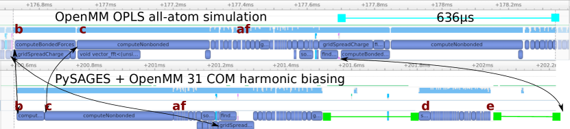
Figure 10: $1.6$ms profiled time line of an Openmm opls simulation of $40,981$ particles as polymers with PME summation for long-range Coulomb forces. The colors and labels are identical to Figure 9. Openmm works with asynchronous GPU kernel execution, which leads to less linearly sorted timelines, compared with hoomd-blue, but we can still identify the CV calculation d) and force biasing e) and the synchronization idle of the GPU (green). Overall, the performance degradation is more pronounced with Openmm compared to hoomd-blue.

In the previous section, we have demonstrated the fast GPU interoperability between pysages and hoomd-blue via jax. However, the concept of pysages is to develop enhanced sampling methods independently of the simulation backend, so here we demonstrate that similar performance can be achieved with Openmm. Since Openmm focuses on all-atom simulations, we simulate an all-atom model of a polymer with the Bigsmiles  [78] notation {[$]CC([$])(C)C(OCC(O)CSC1=CC=C(F)C(F)=C1)=O} with an opls-aa force field [79, 80] including long-range Coulomb forces via PME. We simulate a bulk system of 40mers with 31 macromolecules present, adding up to $40\,981$ atoms. As a proof of concept, we calculated the center of mass for every polymer chain and biased it harmonically via pysages. As a performance metric, we evaluate the ns/day executed on the same hardware configuration as a the hoomd-blue example above. For the unbiased, pure Openmm simulation we achieve a performance of $\approx 136$ ns/day. For the pysages biased simulation, we achieve a performance of $\approx 75$ ns/day, equating to a biasing overhead of approximately $50\%$. Figure 10 shows a similar time series analysis as for hoomd-blue.

It is notable that Openmm’s execution model makes more use of parallel execution of independent kernels, which also changes the order of execution compared to hoomd-blue. As a result, the same CPU synchronization changes the execution more drastically than in hoomd-blue. Additionally, a single time step for this system is faster executed compared to hoomd-blue, making the synchronization overhead more noticeable. In this case, parallelization of pysages and Openmm is projected to have a bigger performance advantage. Furthermore, we notice that the calculation of the center of mass and the biasing of all 31 polymer chains is more costly than the single CV in the previous example. The combination of these factors explain the higher pysages overhead for this Openmm simulation, but overall performance is good and significantly better for alternative implementations that require CV calculations on the CPU.

4 Conclusion

We have introduced pysages, a library for enhanced sampling in molecular dynamics simulations, which allows users to utilize a variety of enhanced sampling methods and collective variables, as well as to implement new ones via a simple Python and jax-based interface.

We showed how pysages can be used through a number of example applications in different fields such as drug design, materials engineering, polymer physics, and ab-initio MD simulations. We hope that these convey for the reader the flexibility and potential of the library for addressing a diverse set of problems in a high-performance manner.

As our analysis showcased, for large problems, pysages can perform biased simulation well over one order of magnitude faster than a library such as SSAGES even when the backend already performs computations on a GPU.

Nevertheless, as with any newly developed software, pysages is still under development and we are continually working to improve it. In the near term, we plan to add the ability for users to perform restarts, which will provide greater flexibility running long simulations. Moreover, we plan to optimize pysages-side computations to run fully asynchronously with the computation of the forces of the backend, which will further enhance its current performance. We also invite the community to contribute to the development of pysages, whether by suggesting new features, reporting bugs, or contributing code.

Overall, we believe that pysages provides a useful tool for researchers interested in performing molecular and ab-initio simulations in multiple fields, due to its user-friendly framework for defining and using sampling methods and collective variables, as well as its high performance on GPU devices.

Looking further ahead, we are excited about the potential for pysages to enable fully end-to-end differentiable free energy calculations. This will provide new possibilities for force-field and materials design, which would drive significant advances in these areas.

Code avalability

The code for pysages is available in the GitHub repository: https://github.com/SSAGESLabs/PySAGES.

Conflict of Interest Statement

A. L. F. is a co-founder and consultant of Evozyne, Inc. and a co-author of US Patent Applications 16/887,710 and 17/642,582, US Provisional Patent Applications 62/853,919, 62/900,420, 63/314,898, and 63/479,378 and International Patent Applications pct/us2020/035206 and pct/us2020/050466.

Appendix A CV for the distance to an interface

Implementation of the CV described in section 2.2.1, that is, the distance between a group of atoms to an interface defined by another group of atoms.

⬇

||

class DistanceToInterface(TwoPointCV):

def __init__(self, indices, axis, sigma, scope, bins=100, coeff=1):

super().__init__(indices)

self.axis = axis

self.sigma = sigma

self.scope = scope

self.bins = bins

self.coeff = coeff

\par@property

def function(self):

return lambda r1, r2: distance_to_interface(

r1, r2, axis=self.axis,

sigma=self.sigma, scope=self.scope,

bins=self.bins, coeff=self.coeff

)

\pardef distance_to_interface(p1, p2, axis, sigma, scope, bins, coeff):

mobile_axis = barycenter(p1)[axis]

positions_axis = p2.flatten()[axis::3]

centers = np.linspace(scope[0], scope[1], bins)

centers = np.expand_dims(centers, 1)

positions_axis = np.expand_dims(positions_axis, 0)

diff = positions_axis - centers

mass = np.exp(-0.5 * (diff / sigma) ** 2)

mass = np.sum(mass, axis=1)

mass_diff = np.abs(mass[1:] - mass[:-1])

centers = np.squeeze(centers)

centers_mean = (centers[1:] + centers[:-1]) / 2

probability = nn.softmax(mass_diff * coeff)

interface = np.sum(probability * centers_mean)

return mobile_axis - interface

||

Appendix B Benchmark test systems

In the following sections, we present the results of the free energy calculation for the benchmark test systems of ADP and butane. The details of all the parameters chosen to perform the enhanced sampling simulation of these are summarized in B.3.

B.1 Alanine Dipeptide

The first test system involves ADP in vacuum (Figure 11), a benchmark system for enhanced sampling methods that is frequently used in the literature.

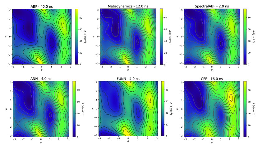
Figure 11: Free energy landscape of alanine dipeptide (Amber f f99sb [81]) in vacuum as a function of the dihedral angles $\phi$ and $\psi$ obtained with pysages and Openmm via different enhanced sampling methods: ABF, Metadynamics, Spectral ABF, ANN, FUNN, CFF. Each panel also indicates the length of the simulation necessary for the free energy to converge. The long ABF simulations represent the ground truth.

B.2 Butane

As a second test system, we compute the free energy profile along the C-C-C-C dihedral angle, $\phi_{CCCC}$, of a butane molecule (in vacuum), Figure 12.

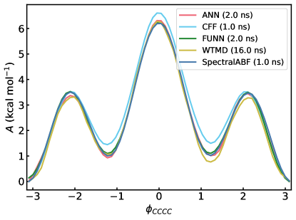
Figure 12: Free energy profile along the dihedral angle of a butane molecule (using an opls-based force field [79]) obtained via different enhanced sampling methods with pysages and hoomd-blue: ANN, CFF, FUNN, Spectral ABF, WTMD. The legend also indicates the length of the simulation. The long ABF simulations represent the ground truth.

B.3 Example System Details

Table 1: Parameters and methods details for the various examples. For all methods but Metadynamics, we used a grid with 50 points along each CV for ADP and with 64 points along the CV for butane.
$N$ (ABF) = Threshold parameter before accounting for the full average of the adaptive biasing force.
ADP = ADP

System	Backend	CV	Method	Settings	Fig.
ADP	Openmm	$\phi$ and $\psi$	ABF	$N=500$ (default)	11
			ANN	$\mathrm{topology}=(8,8)$
			CFF	$\mathrm{topology}=(14,)$
			FUNN	$\mathrm{topology}=(14,)$
			Metadynamics	$\sigma=0.35$ rad
				$h=1.2$ kJ/mol
				stride $=500$
			Spectral ABF	—
Butane	hoomd-blue	$\phi_{CCCC}$	ANN	$\mathrm{topology}=(8,8)$	12
			CFF	$\mathrm{topology}=(8,)$
			FUNN	$\mathrm{topology}=(8,)$
			WTMD	$\sigma=0.10$ rad
				$h=0.01$ kJ/mol
				stride $=50$
				$\Delta T=5000$
			Spectral ABF	—

References

- [1] nobelprize.org, The nobel prize in chemistry 2013 (https://nobelprize.org/prizes/chemistry/2013/summary/, accessed November 2022).
- [2] D. E. Shaw, M. M. Deneroff, R. O. Dror, J. S. Kuskin, R. H. Larson, J. K. Salmon, C. Young, B. Batson, K. J. Bowers, J. C. Chao, et al., Anton, a special-purpose machine for molecular dynamics simulation, Communications of the acm 51 (7) (2008) 91–97.
- [3] D. E. Shaw, J. Grossman, J. A. Bank, B. Batson, J. A. Butts, J. C. Chao, M. M. Deneroff, R. O. Dror, A. Even, C. H. Fenton, et al., Anton 2: raising the bar for performance and programmability in a special-purpose molecular dynamics supercomputer, in: sc’14: Proceedings of the International Conference for High Performance Computing, Networking, Storage and Analysis, ieee, 2014, pp. 41–53.
- [4] J. A. Anderson, J. Glaser, S. C. Glotzer, hoomd-blue: A Python package for high-performance molecular dynamics and hard particle Monte Carlo simulations, Computational Materials Science 173 (2020) 109363.
- [5] P. Eastman, J. Swails, J. D. Chodera, R. T. McGibbon, Y. Zhao, K. A. Beauchamp, L.-P. Wang, A. C. Simmonett, M. P. Harrigan, C. D. Stern, R. P. Wiewiora, B. R. Brooks, V. S. Pande, Openmm 7: Rapid development of high performance algorithms for molecular dynamics, plos Computational Biology 13 (7) (2017) 1–17.
- [6] S. Schoenholz, E. D. Cubuk, jax, m.d. a framework for differentiable physics, in: Advances in Neural Information Processing Systems, Vol. 33, 2020, pp. 11428–11441.
- [7] S. S. Schoenholz, E. D. Cubuk, jax, m.d. a framework for differentiable physics, Journal of Statistical Mechanics: Theory and Experiment 2021 (12) (2021) 124016.
- [8] A. P. Thompson, H. M. Aktulga, R. Berger, D. S. Bolintineanu, W. M. Brown, P. S. Crozier, P. J. in ’t Veld, A. Kohlmeyer, S. G. Moore, T. D. Nguyen, R. Shan, M. J. Stevens, J. Tranchida, C. Trott, S. J. Plimpton, lammps - a flexible simulation tool for particle-based materials modeling at the atomic, meso, and continuum scales, Comp. Phys. Comm. 271 (2022) 108171.
- [9] M. J. Abraham, T. Murtola, R. Schulz, S. Páll, J. C. Smith, B. Hess, E. Lindahl, Gromacs: High performance molecular simulations through multi-level parallelism from laptops to supercomputers, SoftwareX 1 (2015) 19–25.
- [10] G. A. Tribello, M. Bonomi, D. Branduardi, C. Camilloni, G. Bussi, plumed 2: New feathers for an old bird, Computer Physics Communications 185 (2) (2014) 604–613.
- [11] G. Fiorin, M. L. Klein, J. Hénin, Using collective variables to drive molecular dynamics simulations, Molecular Physics 111 (22-23) (2013) 3345–3362.
- [12] H. Sidky, Y. J. Colón, J. Helfferich, B. J. Sikora, C. Bezik, W. Chu, F. Giberti, A. Z. Guo, X. Jiang, J. Lequieu, J. Li, J. Moller, M. J. Quevillon, M. Rahimi, H. Ramezani-Dakhel, V. S. Rathee, D. R. Reid, E. Sevgen, V. Thapar, M. A. Webb, J. K. Whitmer, J. J. de Pablo, ssages: Software suite for advanced general ensemble simulations, The Journal of Chemical Physics 148 (4) (2018) 044104.
- [13] H. Sidky, J. K. Whitmer, Learning free energy landscapes using artificial neural networks, The Journal of Chemical Physics 148 (10) (2018) 104111.
- [14] A. Z. Guo, E. Sevgen, H. Sidky, J. K. Whitmer, J. A. Hubbell, J. J. de Pablo, Adaptive enhanced sampling by force-biasing using neural networks, The Journal of Chemical Physics 148 (13) (2018) 134108.
- [15] E. Sevgen, A. Z. Guo, H. Sidky, J. K. Whitmer, J. J. de Pablo, Combined force-frequency sampling for simulation of systems having rugged free energy landscapes, Journal of Chemical Theory and Computation 16 (3) (2020) 1448–1455.
- [16] D. Wang, Y. Wang, J. Chang, L. Zhang, H. Wang, et al., Efficient sampling of high-dimensional free energy landscapes using adaptive reinforced dynamics, Nature Computational Science 2 (1) (2022) 20–29.
- [17] C. R. Schwantes, V. S. Pande, Improvements in markov state model construction reveal many non-native interactions in the folding of ntl9, Journal of Chemical Theory and Computation 9 (4) (2013) 2000–2009.
- [18] W. Chen, A. L. Ferguson, Molecular enhanced sampling with autoencoders: On-the-fly collective variable discovery and accelerated free energy landscape exploration, Journal of computational chemistry 39 (25) (2018) 2079–2102.
- [19] A. Mardt, L. Pasquali, H. Wu, F. Noé, vampnets for deep learning of molecular kinetics, Nature communications 9 (1) (2018) 1–11.
- [20] W. Chen, H. Sidky, A. L. Ferguson, Capabilities and limitations of time-lagged autoencoders for slow mode discovery in dynamical systems, The Journal of Chemical Physics 151 (6) (2019) 064123.
- [21] W. Chen, H. Sidky, A. L. Ferguson, Nonlinear discovery of slow molecular modes using state-free reversible vampnets, The Journal of Chemical Physics 150 (21) (2019) 214114.
- [22] H. Sidky, W. Chen, A. L. Ferguson, Molecular latent space simulators, Chemical Science 11 (35) (2020) 9459–9467.
- [23] T.-S. Lee, D. S. Cerutti, D. Mermelstein, C. Lin, S. LeGrand, T. J. Giese, A. Roitberg, D. A. Case, R. C. Walker, D. M. York, \AcGPU-accelerated molecular dynamics and free energy methods in Amber18: performance enhancements and new features, Journal of chemical information and modeling 58 (10) (2018) 2043–2050.
- [24] J. C. Phillips, D. J. Hardy, J. D. Maia, J. E. Stone, J. V. Ribeiro, R. C. Bernardi, R. Buch, G. Fiorin, J. Hénin, W. Jiang, et al., Scalable molecular dynamics on cpu and gpu architectures with namd, The Journal of Chemical Physics 153 (4) (2020) 044130.
- [25] C. Kobayashi, J. Jung, Y. Matsunaga, T. Mori, T. Ando, K. Tamura, M. Kamiya, Y. Sugita, genesis 1.1: A hybrid-parallel molecular dynamics simulator with enhanced sampling algorithms on multiple computational platforms (2017).
- [26] C. R. Harris, K. J. Millman, S. J. van der Walt, R. Gommers, P. Virtanen, D. Cournapeau, E. Wieser, J. Taylor, S. Berg, N. J. Smith, R. Kern, M. Picus, S. Hoyer, M. H. van Kerkwijk, M. Brett, A. Haldane, J. F. del Río, M. Wiebe, P. Peterson, P. Gérard-Marchant, K. Sheppard, T. Reddy, W. Weckesser, H. Abbasi, C. Gohlke, T. E. Oliphant, Array programming with NumPy, Nature 585 (7825) (2020) 357–362.
- [27] DLPack (https://github.com/dmlc/dlpack, accessed November 2022).
- [28] trunk.io, Trunk.IO (https://trunk.io, accessed September 2022).
- [29] H. Sidky, W. Chen, A. L. Ferguson, Machine learning for collective variable discovery and enhanced sampling in biomolecular simulation, Molecular Physics 118 (5) (2020) e1737742.
- [30] N. E. Jackson, M. A. Webb, J. J. de Pablo, Recent advances in machine learning towards multiscale soft materials design, Current Opinion in Chemical Engineering 23 (2019) 106–114.
- [31] P. Tiwary, A. v. d. Walle, A review of enhanced sampling approaches for accelerated molecular dynamics, Multiscale materials modeling for nanomechanics (2016) 195–221.
- [32] A.-h. Wang, Z.-c. Zhang, G.-h. Li, Advances in enhanced sampling molecular dynamics simulations for biomolecules, Chinese Journal of Chemical Physics 32 (3) (2019) 277.
- [33] A. Mitsutake, Y. Mori, Y. Okamoto, Enhanced sampling algorithms, Biomolecular Simulations (2013) 153–195.
- [34] Y. Miao, J. A. McCammon, Unconstrained enhanced sampling for free energy calculations of biomolecules: a review, Molecular simulation 42 (13) (2016) 1046–1055.
- [35] Y. I. Yang, Q. Shao, J. Zhang, L. Yang, Y. Q. Gao, Enhanced sampling in molecular dynamics, The Journal of Chemical Physics 151 (7) (2019) 070902.
- [36] C. Abrams, G. Bussi, Enhanced sampling in molecular dynamics using metadynamics, replica-exchange, and temperature-acceleration, Entropy 16 (1) (2014) 163–199.
- [37] V. Limongelli, Ligand binding free energy and kinetics calculation in 2020, wires Computational Molecular Science 10 (4) (2020) e1455.
- [38] G. Piccini, M.-S. Lee, S. F. Yuk, D. Zhang, G. Collinge, L. Kollias, M.-T. Nguyen, V.-A. Glezakou, R. Rousseau, Ab initio molecular dynamics with enhanced sampling in heterogeneous catalysis, Catal. Sci. Technol. 12 (2022) 12–37.
- [39] J. Kästner, Umbrella integration in two or more reaction coordinates, The Journal of Chemical Physics 131 (3) (2009) 034109.
- [40] J. Kästner, Umbrella sampling, Wiley Interdisciplinary Reviews: Computational Molecular Science 1 (6) (2011) 932–942.
- [41] E. Weinan, W. Ren, E. Vanden-Eijnden, Simplified and improved string method for computing the minimum energy paths in barrier-crossing events, Journal of Chemical Physics 126 (16) (2007) 164103.
- [42] J. Comer, J. C. Gumbart, J. Hénin, T. Lelièvre, A. Pohorille, C. Chipot, The adaptive biasing force method: Everything you always wanted to know but were afraid to ask, The Journal of Physical Chemistry B 119 (3) (2015) 1129–1151.
- [43] E. Darve, D. Rodríguez-Gómez, A. Pohorille, Adaptive biasing force method for scalar and vector free energy calculations, The Journal of Chemical Physics 128 (14) (2008) 144120.
- [44] A. Laio, M. Parrinello, Escaping free-energy minima, Proceedings of the National Academy of Sciences 99 (20) (2002) 12562–12566.
- [45] A. Barducci, G. Bussi, M. Parrinello, Well-tempered metadynamics: a smoothly converging and tunable free-energy method, Physical review letters 100 (2) (2008) 020603.
- [46] S. Hussain, A. Haji-Akbari, Studying rare events using forward-flux sampling: Recent breakthroughs and future outlook, The Journal of Chemical Physics 152 (6) (2020) 060901.
- [47] R. J. Allen, P. B. Warren, P. R. ten Wolde, Sampling rare switching events in biochemical networks, Phys. Rev. Lett. 94 (2005) 018104.
- [48] R. J. Allen, D. Frenkel, P. R. ten Wolde, Simulating rare events in equilibrium or nonequilibrium stochastic systems, The Journal of Chemical Physics 124 (2) (2006) 024102.
- [49] J. K. Whitmer, C.-c. Chiu, A. A. Joshi, J. J. De Pablo, Basis function sampling: A new paradigm for material property computation, Physical review letters 113 (19) (2014) 190602.
- [50] P. F. Zubieta Rico, J. J. de Pablo, Sobolev sampling of free energy landscapes, arXiv (2022). arXiv:2202.01876.
- [51] D. Cremer, J. A. Pople, General definition of ring puckering coordinates, Journal of the American Chemical Society 97 (6) (1975) 1354–1358.
- [52] J. M. L. Ribeiro, P. Bravo, Y. Wang, P. Tiwary, Reweighted autoencoded variational bayes for enhanced sampling (rave), The Journal of Chemical Physics 149 (7) (2018) 072301.
- [53] C. Wehmeyer, F. Noé, Time-lagged autoencoders: Deep learning of slow collective variables for molecular kinetics, The Journal of Chemical Physics 148 (24) (2018) 241703.
- [54] W. Wang, Z. Wu, R. Gómez-Bombarelli, Learning pair potentials using differentiable simulations (2022). arXiv:2209.07679.
- [55] A. Sethi, K. Joshi, K. Sasikala, M. Alvala, Molecular docking in modern drug discovery: Principles and recent applications, in: V. Gaitonde, P. Karmakar, A. Trivedi (Eds.), Drug Discovery and Development, Vol. 2, IntechOpen, 2019, Ch. 3, pp. 1–21.
- [56] S. Ruiz-Carmona, P. Schmidtke, F. J. Luque, L. Baker, N. Matassova, B. Davis, S. Roughley, J. Murray, R. Hubbard, X. Barril, Dynamic undocking and the quasi-bound state as tools for drug discovery, Nature Chemistry 9 (3) (2017) 1755–4349.
- [57] M. Majewski, X. Barril, Structural stability predicts the binding mode of protein–ligand complexes, Journal of Chemical Information and Modeling 60 (3) (2020) 1644–1651.
- [58] M. Rachman, D. Bajusz, A. Hetényi, A. Scarpino, B. Merő, A. Egyed, L. Buday, X. Barril, G. M. Keserű, Discovery of a novel kinase hinge binder fragment by dynamic undocking, rsc Med. Chem. 11 (2020) 552–558.
- [59] N. Drayman, J. K. DeMarco, K. A. Jones, S.-A. Azizi, H. M. Froggatt, K. Tan, N. I. Maltseva, S. Chen, V. Nicolaescu, S. Dvorkin, K. Furlong, R. S. Kathayat, M. R. Firpo, V. Mastrodomenico, E. A. Bruce, M. M. Schmidt, R. Jedrzejczak, M. A. Munoz-Alia, B. Schuster, V. Nair, K. yeon Han, A. O’Brien, A. Tomatsidou, B. Meyer, M. Vignuzzi, D. Missiakas, J. W. Botten, C. B. Brooke, H. Lee, S. C. Baker, B. C. Mounce, N. S. Heaton, W. E. Severson, K. E. Palmer, B. C. Dickinson, A. Joachimiak, G. Randall, S. Tay, Masitinib is a broad coronavirus 3cl inhibitor that blocks replication of sars-cov-2, Science 373 (6557) (2021) 931–936.
- [60] S. Ruiz-Carmona, D. Alvarez-Garcia, N. Foloppe, A. B. Garmendia-Doval, S. Juhos, P. Schmidtke, X. Barril, R. E. Hubbard, S. D. Morley, rdock: A fast, versatile and open source program for docking ligands to proteins and nucleic acids, plos Computational Biology 10 (4) (2014) 1–7.
- [61] J. A. Maier, C. Martinez, K. Kasavajhala, L. Wickstrom, K. E. Hauser, C. Simmerling, f f14sb: Improving the accuracy of protein side chain and backbone parameters from f f99sb, Journal of Chemical Theory and Computation 11 (8) (2015) 3696–3713.
- [62] W. L. Jorgensen, J. Chandrasekhar, J. D. Madura, R. W. Impey, M. L. Klein, Comparison of simple potential functions for simulating liquid water, J. Chem. Phys. 79 (2) (1983) 926–935.
- [63] J. Wang, R. M. Wolf, J. W. Caldwell, P. A. Kollman, D. A. Case, Development and testing of a general amber force field, J. Comput. Chem. 25 (9) (2004) 1157–1174.
- [64] D. A. Case, K. Belfon, I. Y. Ben-Shalom, S. R. Brozell, D. S. Cerutti, T. E. Cheatham, III, V. W. D. Cruzeiro, T. A. Darden, R. E. Duke, G. Giambasu, M. K. Gilson, H. Gohlke, A. W. Goetz, R. Harris, S. Izadi, S. A. Izmailov, K. Kasavajhala, A. Kovalenko, R. Krasny, T. Kurtzman, T. S. Lee, S. LeGrand, P. Li, C. Lin, J. Liu, T. Luchko, R. Luo, V. Man, K. M. Merz, Y. Miao, O. Mikhailovskii, G. Monard, H. Nguyen, A. Onufriev, F. Pan, S. Pantano, R. Qi, D. R. Roe, A. Roitberg, C. Sagui, S. Schott-Verdugo, J. Shen, C. L. Simmerling, N. R. Skrynnikov, J. Smith, J. Swails, R. C. Walker, J. Wang, L. Wilson, R. M. Wolf, X. Wu, Y. Xiong, Y. Xue, D. M. York, P. A. Kollman, Amber 2020 (2020).
- [65] L. Schneider, M. Heck, M. Wilhelm, M. Müller, Transitions between lamellar orientations in shear flow, Macromolecules 51 (12) (2018) 4642–4659.
- [66] L. Schneider, M. Müller, Rheology of symmetric diblock copolymers, Computational Materials Science 169 (2019) 109107.
- [67] L. Schneider, G. Lichtenberg, D. Vega, M. Müller, Symmetric diblock copolymers in cylindrical confinement: A way to chiral morphologies?, acs Applied Materials & Interfaces 12 (44) (2020) 50077–50095.
- [68] M. W. Matsen, The standard gaussian model for block copolymer melts, Journal of Physics: Condensed Matter 14 (2) (2001) R21.
- [69] Z. Wang, T. Xu, A. Noel, Y.-C. Chen, T. Liu, Applications of liquid crystals in biosensing, Soft Matter 17 (2021) 4675–4702.
- [70] H. Ramezani-Dakhel, M. Sadati, M. Rahimi, A. Ramirez-Hernandez, B. Roux, J. J. de Pablo, Understanding atomic-scale behavior of liquid crystals at aqueous interfaces, Journal of Chemical Theory and Computation 13 (1) (2017) 237–244.
- [71] G. Tiberio, L. Muccioli, R. Berardi, C. Zannoni, Towards in silico liquid crystals. realistic transition temperatures and physical properties for n-cyanobiphenyls via molecular dynamics simulations, ChemPhysChem 10 (1) (2009) 125–136.
- [72] J. P. Perdew, K. Burke, M. Ernzerhof, Generalized gradient approximation made simple [Phys. Rev. Lett. 77, 3865 (1996)], Phys. Rev. Lett. 78 (1997) 1396–1396.
- [73] L. Zhang, J. Han, H. Wang, R. Car, W. E, Deep potential molecular dynamics: A scalable model with the accuracy of quantum mechanics, Phys. Rev. Lett. 120 (2018) 143001.
- [74] M. Yang, L. Bonati, D. Polino, M. Parrinello, Using metadynamics to build neural network potentials for reactive events: the case of urea decomposition in water, Catalysis Today 387 (2022) 143–149, 100 years of casale sa: a scientific perspective on catalytic processes.
- [75] D. Unruh, R. V. Meidanshahi, S. M. Goodnick, G. Csányi, G. T. Zimányi, Gaussian approximation potential for amorphous si : H, Phys. Rev. Materials 6 (2022) 065603.
- [76] E. D. Cubuk, B. D. Malone, B. Onat, A. Waterland, E. Kaxiras, Representations in neural network based empirical potentials, The Journal of Chemical Physics 147 (2) (2017) 024104.
- [77] R. Frostig, M. J. Johnson, C. Leary, Compiling machine learning programs via high-level tracing, Systems for Machine Learning 4 (9) (2018).
- [78] T.-S. Lin, C. W. Coley, H. Mochigase, H. K. Beech, W. Wang, Z. Wang, E. Woods, S. L. Craig, J. A. Johnson, J. A. Kalow, et al., Bigsmiles: a structurally-based line notation for describing macromolecules, acs Central Science 5 (9) (2019) 1523–1531.
- [79] W. L. Jorgensen, D. S. Maxwell, J. Tirado-Rives, Development and testing of the opls all-atom force field on conformational energetics and properties of organic liquids, Journal of the American Chemical Society 118 (45) (1996) 11225–11236.
- [80] L. Schneider, M. Schwarting, J. Mysona, H. Liang, M. Han, P. M. Rauscher, J. M. Ting, S. Venkatram, R. B. Ross, K. J. Schmidt, B. Blaiszik, I. Foster, J. J. de Pablo, In silico active learning for small molecule properties, Mol. Syst. Des. Eng. (2022).
- [81] V. Hornak, R. Abel, A. Okur, B. Strockbine, A. Roitberg, C. Simmerling, Comparison of multiple amber force fields and development of improved protein backbone parameters, Proteins: Structure, Function, and Bioinformatics 65 (3) (2006) 712–725.