Phase-shifted Adversarial Training

Abstract

Adversarial training (AT) has been considered an imperative component for safely deploying neural network-based applications. However, it typically comes with slow convergence and worse performance on clean samples (i.e., non-adversarial samples). In this work, we analyze the behavior of neural networks during learning with adversarial samples through the lens of response frequency. Interestingly, we observe that AT causes neural networks to converge slowly to high-frequency information, resulting in highly oscillatory predictions near each data point. To learn high-frequency content efficiently, we first prove that a universal phenomenon, the frequency principle (i.e., lower frequencies are learned first), still holds in AT. Building upon this theoretical foundation, we present a novel approach to AT, which we call phase-shifted adversarial training (PhaseAT). In PhaseAT, the high-frequency components, which are a contributing factor to slow convergence, are adaptively shifted into the low-frequency range where faster convergence occurs. For evaluation, we conduct extensive experiments on CIFAR-10 and ImageNet, using an adaptive attack that is carefully designed for reliable evaluation. Comprehensive results show that PhaseAT substantially improves convergence for high-frequency information, thereby leading to improved adversarial robustness.

1 Introduction

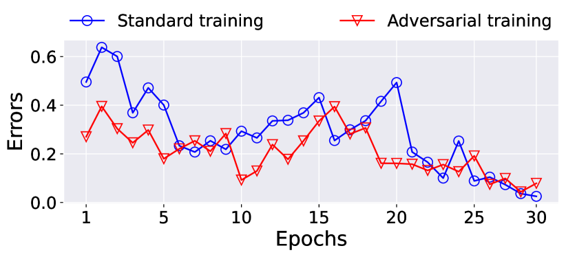
(a)

(b)

Figure 1: Errors of frequency components (high, low) between the training dataset and neural networks. Here, we use CIFAR-10 dataset for validation.

Despite the remarkable success, deep neural networks are known to be susceptible to crafted imperceptible noise called adversarial attacks [Szegedy et al., 2013], which can have severe consequences when deployed in critical applications such as self-driving cars, medical diagnosis, and surveillance systems. In response to such negative implications, there has been a recent surge in research aimed at preventing adversarial attacks, such as adversarial training [Madry et al., 2018, Wong et al., 2020, Sriramanan et al., 2020, 2021], data augmentation [Gong et al., 2021, Wang et al., 2021, Rebuffi et al., 2021], and regularization [Qin et al., 2019]. Adversarial training is considered one of the most effective ways to achieve adversarial robustness. The early attempt generates the attack by only a single gradient descent on the given input, which is known as fast gradient sign method (FGSM) [Goodfellow et al., 2015]. However, it was later shown to be ineffective against strong multiple-step attacks [Kurakin et al., 2016], e.g., projected gradient descent (PGD). Hence a myriad of defense strategies are introduced to build the robust models against the strong attacks by injecting the regularization to the perturbations [Sriramanan et al., 2020, 2021], randomly initializing the perturbations [Wong et al., 2020, Tramer and Boneh, 2019], and increasing the number of update steps for the perturbation to approximate the strong attack [Madry et al., 2018, Zhang et al., 2019].

Instead of introducing new attack and defense strategies, we analyze adversarial training through the lens of the frequency of the general mapping between inputs and outputs (e.g., neural networks). For this purpose, we calculate the errors of the frequency components between the dataset and neural networks to observe how the networks converge to the labeling function of the training dataset in terms of the frequencies. Compared to standard training (blue dots in Figure 1), we find that adding adversarial examples (red inverted triangles in Figure 1) causes the model to slowly converge in the high-frequency components (Figure 1(b)). This indicates that adversarial robustness comes at significantly increased training time compared to standard training.

To learn high-frequency contents of the dataset efficiently, phase-shift deep neural networks (PhaseDNN) [Cai et al., 2020] is proposed based on a universal phenomenon of frequency principle (F-principle) [Xu et al., 2019, 2020b, Rahaman et al., 2019, Luo et al., 2021], that is, deep neural networks often fit target functions from low to high frequencies during the training. PhaseDNN learns high-frequency contents by shifting these frequencies to the range of low-frequency to exploit the faster convergence in the low-frequencies of the DNN. However, it is challenging to apply PhaseDNN to adversarial training because PhaseDNN was optimized to solve a single-dimensional data (e.g., electromagnetic wave propagation, seismic waves).

In this work, we propose phase-shifted adversarial training (PhaseAT) to achieve adversarial robustness efficiently and effectively. To this end, we theoretically prove that the F-principle holds not only in standard training but also in adversarial training. We then extend the phaseDNN to adopt high-dimensional data and learn the adversarial data effectively. In summary, our contributions include the following:

• We conduct a pioneering analysis of adversarial training from the perspective of response frequency.

• We establish a mathematical foundation for how adversarial training behaves by considerably extending a universal phenomenon of frequency principle.

• We propose a new phase-shifted adversarial training algorithm based on our proposed theory, outperforming other strong baselines in many different settings.

2 Background of Adversarial Training

Adversarial training is a method for learning networks that are robust to adversarial attacks. Given a network $\mathcal{T}$ parameterized by $\theta$, a dataset $\{x_{j},y_{j}\}_{j=0}^{N-1}$ where $N$ is the size of dataset, a loss function $\ell$ and a threat model $\Delta$, the learning problem can be cast to the following robust optimization problem.

$$\min_{\theta}\sum_{j=0}^{N-1}\max_{\delta\in\Delta}\ell(\mathcal{T}(x_{j}+\delta),y_{j})$$ (2.1)

where $\delta$ is the adversarial perturbation. As we consider the adversarial robustness against $L_{\infty}$ constrained adversaries, the threat model $\Delta$ takes the perturbation $\delta$ such that $\|\delta\|_{\infty}\leq\epsilon$ for some $\epsilon>0$. For adversarial training, it is common to use adversarial attack to approximate the inner maximization over $\Delta$, followed by some variation of gradient descent on the model parameters $\theta$. For example, FGSM attack [Goodfellow et al., 2015] has the following approximation.

$$\delta=\epsilon\cdot\text{sign}(\nabla_{x}\ell(\mathcal{T}(x_{j}),y_{j}))$$ (2.2)

3 F-principle in Adversarial Training

This section is devoted to theoretically demonstrating the F-principle in adversarial training as well as standard training (i.e., $\delta=0$). We first represent the total loss $L(\theta)$ in the frequency domain and then quantify the rate of change of $L(\theta)$ contributed by high frequencies. We provide detailed proof in Supplementary material.

3.1 The total loss in the frequency domain

Given a dataset $\{x_{j},y_{j}\}_{j=0}^{N-1}$, $\mathcal{T}_{\theta}$ is the DNN output and $g(x)$ is the target function (also known as labeling function) such that $g(x_{j})=y_{j}$. Then the total loss $L$ is generally defined by

$$L(\theta)=\frac{1}{N}\sum_{j=0}^{N-1}\ell(\mathcal{T}_{\theta},g)(x_{j}).$$

Here, for example, $\ell(\mathcal{T}_{\theta},g)(x)=\|\mathcal{T}_{\theta}(x)-g(x)\|^{2}$ for mean-squared error loss function, and for cross-entropy loss function $\ell(\mathcal{T}_{\theta},g)(x)=-g(x)\cdot\log\mathcal{T}_{\theta}(x)$ where the log function acts on each vector component of $\mathcal{T}_{\theta}$. In adversarial training, we define an adversarial function $\mathcal{A}:\mathbb{R}^{d}\rightarrow\mathbb{R}^{d}$ by $\mathcal{A}(x)=x+\delta(x)$ with the adversarial perturbation $\delta$ and the corresponding output is given by $\mathcal{T}_{\theta}\circ\mathcal{A}$. In reality, it may be considered that $\mathcal{T}_{\theta}$ and $g$ are bounded in a compact domain containing $\{x_{j}\}_{j=0}^{N-1}$. Then for the two common examples, $\ell(\mathcal{T}_{\theta}\circ\mathcal{A},g)$ is absolutely integrable and $\ell(\mathcal{T}_{\theta}\circ\mathcal{A},g)$ is differentiable with respect to the first argument. In this regard, these properties are considered to be possessed by a loss function generally.

Theorem 3.1.

Let $\widehat{f}$ denote the Fourier transform of $f$. Then, in the frequency domain

$$L(\theta)=\lim_{\varepsilon\rightarrow 0}\frac{1}{N}\sum_{j=0}^{N-1}\int_{\mathbb{R}^{d}}e^{2\pi ix_{j}\cdot\xi}e^{-\pi\|\varepsilon\xi\|^{2}}\savestack{\tmpbox}{\stretchto{\scaleto{\scalerel*[width("\ell(\mathcal{T}_{\theta}\circ\mathcal{A},g)")]{\kern 0.1pt\mathchar 866\relax\kern 0.1pt}{\rule{0.0pt}{505.89pt}}}{}}{2.4ex}}\stackon[-6.9pt]{\ell(\mathcal{T}_{\theta}\circ\mathcal{A},g)}{\tmpbox}(\xi)d\xi.$$ (3.1)

This representation is inspired by a convergence property, $G_{\varepsilon}\ast L(\theta)\rightarrow L(\theta)$, of convolution with approximate identities $G_{\varepsilon}(x):=\varepsilon^{-d}e^{-\pi\|\varepsilon^{-1}x\|^{2}}$. See Lemma D.1 in Supplementary material.

Now we split the integral in Eq. 3.1 into the region $\|\xi\|\leq\eta$ and $\|\xi\|\geq\eta$ for any $\eta>0$ to separate the total loss into two parts $L_{\leq\eta}(\theta)$ and $L_{\geq\eta}(\theta)$ contributed by low and high frequencies, respectively:

$$L(\theta)=\lim_{\varepsilon\rightarrow 0}\big{(}L_{\leq\eta}(\theta)+L_{\geq\eta}(\theta)\big{)}.$$ (3.2)

3.2 Quantifying the rate of change in total loss

Let $W^{s,\infty}(\mathbb{R}^{d})$ denote the Sobolev spaces which consist of bounded functions having bounded derivatives up to a given order $s$, and thus the index $s$ reflects the degree of regularity.

Theorem 3.2.

Consider a DNN with multi-layer in adversarial training. If an activation function $\sigma$ and the target function $g$ satisfy $\sigma\in W^{s,\infty}(\mathbb{R})$ and $g\in W^{2s,\infty}(\mathbb{R}^{d})$ for some $s\in\mathbb{N}$, then there exists a constant $C>0$ independent of $s,\eta$ such that for any $\eta>0$

$$\|\nabla_{\theta} L(\theta)-\nabla_{\theta}L_{\leq\eta}(\theta)\|$$

$$\qquad\,\,\approx\|\nabla_{\theta}L_{\geq\eta}(\theta)\|\leq C\max\{N,d^{d}\}\eta^{-2s}.$$ (3.3)

Theorem 3.2 implies that the rate of decrease in the corresponding high-frequency region loss ($L_{\geq\eta}(\theta)$) is much greater than the rate of increase in $\eta$. In other words, a model tends to fit target functions from low to high frequency information during the adversarial training. The mathematical insight of this theorem is that the regularity of a network converts into the decay of the total loss in the frequency domain. Specifically, a network with a more regular activation function (bigger $s$) converges more slowly, according to $\eta^{-2s}$ in Eq. 3.2. As the frequency increases, this becomes more evident. For example, if $\sigma$ is ReLU or eLu then $s=1$ or $s=2$, respectively. For $\tanh$ and sigmoid activation functions, $s$ may be taken arbitrarily large.

The approximation in Eq. 3.2 becomes more accurate as $\varepsilon$ diminishes in Eq. 3.2, and $\varepsilon=\min\{1/\sqrt[d]{N},1/d\}$ is inversely proportional to the size of dataset ($N$) or the dimension of input data ($d$). Therefore, when $N$ or $d$ are large, $\varepsilon$ decreases. This is a common phenomenon in real-world datasets, which are typically high-dimensional and contain a large number of data samples (e.g., images and languages).

Our innovative theory differs from its predecessors [Xu et al., 2020b, Luo et al., 2021] in two ways. First, we generalize F-principle by showing that it holds for the cross-entropy loss. Second, we provide a faster decay rate with $2s$ in Eq. 3.2, which serves as one of the motivations for using phase-shifting, particularly in adversarial training. Finally, we provide the mathematical justification for the F-principle in adversarial training settings.

4 Phase-shifted Adversarial Training

In this section, we detail the proposed method, coined phase-shifted adversarial training (PhaseAT). We first present the existing PhaseDNN [Cai et al., 2020] and its limitations (Section 4.1). We then redesign the original PhaseDNN to make it more practical and suitable for adversarial training (Section 4.2). Finally, we elaborate PhaseAT by optimizing PhaseDNN through adversarial training (Section 4.3).

4.1 Phase Shift Deep Neural Networks

To learn highly oscillatory functions efficiently, [Cai et al., 2020] propose PhaseDNN which shifts the high-frequency components of the dataset to the range of the low-frequency range for fast convergence because according to F-principle, neural networks learn low-frequency information first before learning high-frequency components. On the phase-shifted dataset, the neural networks learn the target function with low-frequency contents. Unfortunately, this requires that the frequency extraction of the original training data has to be done numerically using convolutions with a frequency selection kernel, which requires a huge memory footprint, i.e., a storage of $O$(N × N). Alternatively, the neural networks can be learned on the data from all ranges of frequencies while the phase-shift is included in the makeup of the PhaseDNN. This version of PhaseDNN is called coupled PhaseDNN, and we adopt this version to avoid the cost of decomposing the frequency components on the original dataset.

Since the phase-shift is performed on the networks rather than the dataset, PhaseDNN consists of an ensemble of networks, each of which is dedicated to a specific frequency. To learn higher frequency components, phase-shift is applied to each network separately. The output of PhaseDNN can be represented as follows:

$$\mathcal{T}(x)=\sum_{m=0}^{M-1}e^{i\omega_{m}x}\cdot\mathcal{T}_{m}(x)$$ (4.1)

where $M$ is the size of ensemble, $T_{m}(x)$ represents one of the networks in the ensemble, and $\omega_{m}$ is the specific frequency for the networks $T_{m}$. Let the labeling function of the dataset be $g(\cdot)$, the phaseDNN is optimized by following the least square errors:

$$\sum_{j=0}^{N-1}|g(x_{j})-\mathcal{T}(x_{j})|^{2}=\sum_{j=0}^{N-1}\left|g(x_{j})-\sum_{m=0}^{M-1}e^{i\omega_{m}x_{j}}\cdot\mathcal{T}_{m}(x_{j})\right|^{2}$$ (4.2)

Note that we always include the lowest frequency in the selected frequency, i.e., $\omega_{0}=0$, because the low frequencies typically dominates in real datasets [Xu et al., 2020b].

4.2 Multi-headed PhaseDNN

Applying the previous PhaseDNN to adversarial training has a few challenges. First, PhaseDNN was designed to learn single-dimensional data; the number of all possible frequencies grows exponentially with the dimension of the input, which prevents the use of high-dimensional inputs (e.g., images and languages). Second, PhaseDNN requires multiple networks to perform the phase-shift of the different frequencies, causing a large memory footprint.

To address the first challenge, we project the given inputs to the first principal component and use the projected scalar values to represent the original data. The forward propagation of PhaseDNN (Eq. 4.1) is reformulated as:

$$\mathcal{T}(x_{j})=\sum_{m=0}^{M-1}e^{i\omega_{m}(x_{j}\cdot p)}\cdot\mathcal{T}_{m}(x_{j})$$ (4.3)

where $p$ is the first principal component of the input space calculated on the training dataset. Instead of observing all frequencies of high-dimensional data, we focus on the frequencies of the data along the first principal component $p$. Additionally, we bound the product result by normalizing the two vectors (i.e., $x$ and $p$) and multiplying the constant $C$ to fix the range of data points.

Lastly, we introduce a multi-headed PhaseDNN to avoid using the ensemble, which consumes large computational resources. We make each network $\mathcal{T}_{m}$ share the feature extracting networks and has frequency-dedicated networks for predictions. Thus, Eq 4.3 is reformulated as follows:

$$\mathcal{T}(x_{j})=\sum_{m=0}^{M-1}e^{i\omega_{m}(x_{j}\cdot p)}\cdot\mathcal{H}_{m}(\mathcal{F}(x_{j}))$$ (4.4)

where $\mathcal{F}(\cdot)$, $\mathcal{H}_{m}(\cdot)$ are the shared networks and the $m$-th frequency-dedicated classifier, respectively. It is worth noting that the classifiers $\mathcal{H}$ only make up a small portion of the total parameters, allowing PhaseDNN to efficiently learn highly oscillatory functions with a lower memory footprint.

4.3 PhaseDNN with Adversarial Training

PhaseDNN requires shift frequencies ($\{\omega_{m}\}_{m=0}^{M-1}$) for each head ($\{\mathcal{H}_{m}\}_{m=0}^{M-1}$) used during training. The following explains how to choose those frequencies. As the goal of training a network is to minimize the differences between a clean ($\{x_{j}\}_{j=0}^{N-1}$) and an adversarial version ($\{x_{j}=x_{j}+\delta\}_{j=0}^{N-1}$) of the same data point, we choose the target frequencies with the largest difference in Fourier coefficients between the two. In practice, estimating the Fourier coefficients of the total dataset in every optimization step requires huge computational resources; therefore, we approximate this by estimating the exponential moving average of the coefficients on mini batches. The discrepancy of the frequency $k$ between clean and adversarial batches is determined as follows:

$${d}_{k}=\left|\mathcal{F}_{k}(X)-\mathcal{F}_{k}(X+\Delta)\right|$$ (4.5)

where $X$ and $\Delta$ indicate the batched data and its corresponding perturbations, respectively, $\mathcal{F}_{k}(\cdot)$ is the Fourier coefficient which is obtained as follows:

$$\mathcal{F}_{k}(X)=\sum_{j=0}^{B-1}\mathcal{T}(X_{j})\cdot e^{-2\pi ik(X_{j}\cdot p)}$$ (4.6)

where $B$ is the batch size. The estimated discrepancy $d_{k}$ for all frequencies is then used to derive the multinomial distribution to sample the frequencies $\omega_{m}$ for each head of the phaseDNN. The reason for sampling frequencies from a multinomial distribution is that the training dataset is constantly changing during adversarial training. In this case, a fixed set of frequencies (e.g., peaks of frequencies used in [Xu et al., 2020b]) does not accurately reflect the critical frequency information. As a result, by stochastically learning the frequency differences, the model could decrease the prediction differences between clean and adversarial data.

Attack generation.

With the practically-designed PhaseDNN, we perform adversarial training, which causes the neural networks to highly oscillate near the training data. Motivated by the recent finding that FGSM-based training can sufficiently prevent strong attacks [Wong et al., 2020], we train PhaseDNN to be robust against FGSM attacks.

Algorithm 1 Phase-shifted Adversarial Training

1:Training epochs $T$, dataset $\mathcal{D}$, dataset size $N$, perturbation size $\epsilon$, perturbation step $\alpha$, networks $\mathcal{T}$

2:for $t=1$ $...$ $T$ do

3:     for each  Batch $(X,Y)\sim\mathcal{D}$  do

4:         $\Delta=$ Uniform$(-\epsilon,\epsilon)$

5:         // Alternate training across mini-batches

6:         if $j$ % 2 == 0 then

7:              $\Delta=\Delta+\alpha\cdot$ sign($\nabla_{\Delta}\ell_{\text{ce}}(\mathcal{T}(X+\Delta),Y)$)

8:         else

9:              $\Delta=\Delta+\alpha\cdot$ sign($\nabla_{\Delta}\ell_{\text{ce}}(\mathcal{T}_{0}(X+\Delta),Y)$)

10:         end if

11:         $\Delta=$ max(min($\Delta,\epsilon$), $-\epsilon$)

12:         // Sampling frequencies for $\mathcal{T}$ (Eq. (4.5), (4.6))

13:         ${d}=\left|\mathcal{F}(X)-\mathcal{F}(X+\Delta)\right|$

14:         $\{\omega_{m}\}_{m=1}^{M}\sim\text{Multinomial}(d)$

15:         // Optimize networks based on loss (Eq. (4.7)

16:         $\theta=\theta-\nabla_{\theta}[\ell_{\text{adv}}(X,Y)$)]

17:     end for

18:end for

The FGSM attack is formulated by initializing the perturbation on uniform distribution ranging ($-\epsilon$, $\epsilon$). The perturbation is then updated based on the sign of the gradients of the cross-entropy with the ground-truth labels. Since PhaseDNN selects the frequencies in a stochastic manner, the generated attack can encourage PhaseDNN to better fit the diverse components having high-frequencies (detailed in Section 5.2). Moreover, we perform the phase-shift in alternate mini-batches which further diversifies the attacks used for adversarial training similar to the previous studies [Sriramanan et al., 2020, 2021].

Adversarial training.

We improve the model’s robustness against generated attacks by replacing the clean inputs with perturbed ones during training. Additional improvements can be achieved by regularization to minimize the effects of potential white-box attacks. One possible white-box attack would set all shift frequencies to zero, resulting in gradients similar to normal AT rather than PhaseAT. Our regularization term encourages the model to behave differently than the standard AT. We implement this by minimizing the prediction similarity between the phase-shifted model and the model that does not have the phase-shift. In summary, the total objective function is the sum of the cross-entropy loss and the regularization.

$$\ell_{adv}(x,y) =\ell_{ce}(\mathcal{T}(x+\delta),y)\text{ }+$$ (4.7)

$$\left|\frac{\sigma(\mathcal{T}(x+\delta))\cdot\sigma(\mathcal{T}_{0}(x+\delta))}{\|\sigma(\mathcal{T}(x+\delta))\|\|\sigma(\mathcal{T}_{0}(x+\delta))\|}\right|$$

where $\ell_{ce}$ is the cross entropy function, $\sigma$ indicates softmax function, $\mathcal{T}_{0}$ indicates the model without the phase-shift term (i.e., $\omega_{m}=0,$ $\forall$ $m\in[1,M]$). By encouraging the model to have different predictions than normal AT, the model achieves robustness against the normal AT attack as well The proposed defense is detailed in Algorithm-1.

5 Evaluations

5.1 Experimental Setup

Baselines.

We compare our method with both non-iterative and iterative methods. Non-iterative methods updates the perturbation once to generate the attacks, whereas iterative methods generate the perturbations through multiple optimization steps. We choose three recent non-iterative methods for comparison, namely FBF [Wong et al., 2020], GAT[Sriramanan et al., 2020], and NuAT [Sriramanan et al., 2021]. For iterative methods, we select four representative baselines, i.e., PGD [Madry et al., 2018], TRADES [Zhang et al., 2019], GAIRAT [Zhang et al., 2020], and AWP [Wu et al., 2020]. We carefully set the hyper-parameters for the aforementioned methods. We use ResNet-18 [He et al., 2016] and WideResNet-34-10 [Zagoruyko and Komodakis, 2016] architectures [He et al., 2016] for the evaluations and, the detailed settings are listed in Supplementary material.

Datasets and Evaluations.

Following recent works, we perform experiments on two datasets: CIFAR-10 [Krizhevsky et al., 2009] and ImageNet [Deng et al., 2009]. To compare with the recent works, we use ImageNet-100 [Sriramanan et al., 2020, 2021] which is the small version of ImageNet including 100 classes. To evaluate adversarial robustness, we consider both white-box and black-box attacks. For white-box attacks, PGD and AutoAttack (AA) are mainly used, each of which contains $L_{\infty}$ adversarial constraint of $\epsilon=8/255$. Specifically, the AA attacks involve APGD_ce, APGD_dlr, APGD_t [Croce and Hein, 2020b] and FAB_t [Croce and Hein, 2020a]. The black-box attacks include transfer-based and query-based attacks. For the transfer-based attack, we generate PGD-7 perturbations using other networks (e.g., VGG-11 and ResNet-18 that is differently initialized) to attack each baseline. For query-based attacks, we use square attacks [Andriushchenko et al., 2020] with 5,000 query budgets. The results of black-box attacks are included in Supplementary material.

Table 1: Performance evaluation of the different designs of adaptive attacks on CIFAR-10 dataset.

Attack Accuracy PGD₅₀ 61.5 PGD₅₀ + EOT 60.9 PGD₅₀ + Frequency 59.7 PGD₅₀ + EOT + Frequency 59.5

Table 2: Performance evaluation on CIFAR-10 dataset against white-box attacks on two different architectures. Best and second best results are highlighted in boldface and underline, respectively.

Method	Clean accuracy	PGD50+EOT	AA+EOT
Normal	93.1	0.0	0.0
FBF	84.0	43.8	41.0
GAT	80.5	53.2	47.4
NuAT	81.6	52.0	48.3
PhaseAT (ours)	86.2	59.5	52.1
PGD-AT	81.3	50.8	47.3
TRADES	79.5	52.2	48.5
GAIRAT	82.7	56.3	34.5
AWP	81.8	54.8	51.1

(a) ResNet-18

Method	Clean accuracy	PGD50+EOT	AA+EOT
Normal	94.5	0.0	0.0
FBF	82.1	54.4	51.3
GAT	84.7	56.1	52.1
NuAT	85.1	54.6	53.1
PhaseAT (ours)	88.8	62.3	59.2
PGD-AT	86.7	56.8	54.7
TRADES	87.6	55.9	53.9
GAIRAT	85.3	57.6	42.6
AWP	86.9	60.4	56.5

(b) WideResNet-34-10

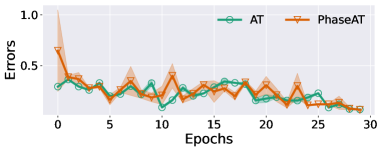
(a)

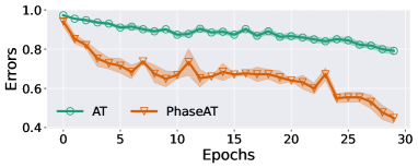
(b)

Figure 2: Errors of frequency components (high, low) between the training dataset and neural networks for normal adversarial training method and PhaseAT.

Consideration of Adaptive Attack.

Compared to previous methods, PhaseAT includes stochastic process to learn diverse frequencies of the datasets, which prevents reliable evaluation of the adversarial robustness. Following the guideline [Tramèr et al., 2018], we carefully design the adaptive attack for our method. First, to circumvent the stochastic process, the adaptive attack involves the expectation over transformation (EOT) [Athalye et al., 2018] to approximate the true gradient of the inference model. Second, we assume that the adversary has full knowledge of the learning algorithm. Hence the adversary could mimic the strategy of frequency selection used in the training/inference phase, i.e., multinomial distribution of the discrepancy. We tabulate how these adaptive attacks affect our method in Table 1.

This shows that reducing the effect of the stochastic properties by EOT decreases the performance of our method. Particularly, mimicking the frequency selection strategy further reduces the performance. However, note that PhaseAT still reveals strong adversarial robustness even though the adaptive attacks are applied (refer to main paper), which requires ten times more costs to generate the attacks compared to other baselines. Such adaptive attacks are applied to our method for a fair comparison.

5.2 Main Results against White-box Attacks

Before comparing the performance of all methods, we first verify whether our method learns high-frequency components faster than the model without the phase-shift. To that end, we use the filtering method [Xu et al., 2020b] used in previous analysis (Figure 1). Figure 2 shows the errors for each frequency. Here, we use the settings of CIFAR-10. For the low-frequency part, the errors between PhaseAT and AT are negligible, whereas the errors of the high-frequency between two methods is noticeable, demonstrating our hypothesis that PhaseAT can efficiently learn high-frequency components.

We then confirm that fast learning of high-frequency components leads to better robustness. Table 2(b) shows the comparison results. Here, we use the two different networks, ResNet-18 and WideResNet-34-10, to verify the generality of PhaseAT. Non-iterative methods tend to show lower accuracy than iterative methods. However, the non-iterative version of PhaseAT outperforms iterative baselines in terms of both standard and robust accuracy. For example, PhaseAT shows 5.3% and 8.5% performance improvement over AWP in terms of standard and PGD accuracy, respectively, and comparable performance for AA. In the experimental results, PhaseAT outperforms FBF, the major distinction of which is the phase-shift functionality. This suggests that learning high-frequency information properly is particularly beneficial for learning adversarial data.

We turn our focus to a larger dataset, i.e., ImageNet. We compare our method with all non-iterative methods and tabulate the results in Table 3. We again find a similar trend in performance to that of CIFAR-10 except for the strongest baseline is the non-iterative method (i.e., NuAT). While the proposed method shows the comparable performance for clean accuracy, it outperforms others by a large margin in terms of the robust accuracy against the AA attack. This shows that PhaseAT can be scalable to larger datasets.

Table 3: Performance evaluation on ImageNet-100 dataset against white-box attacks. Best and second best results are highlighted in boldface and underline, respectively. The results for each baseline come from the previous works [Sriramanan et al., 2020, 2021].

Method Clean accuracy AA+EOT Normal 77.1 0.0 FBF 70.5 20.4 GAT 68.0 28.9 NuAT 69.0 32.0 PhaseAT (ours) 69.2 35.6 PGD-AT 68.6 33.0 TRADES 62.9 31.7 AWP 64.8 29.2

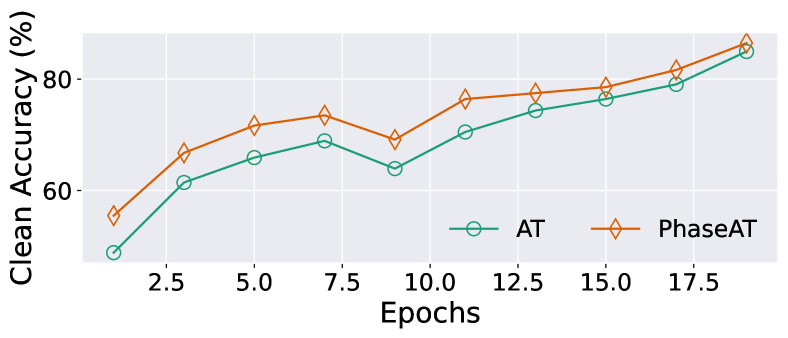
(a)

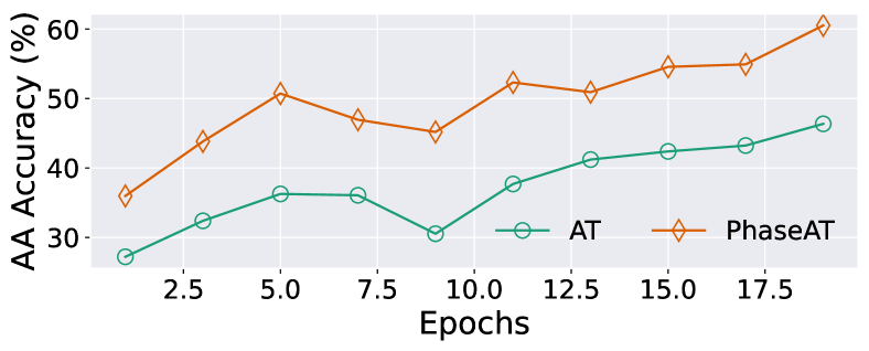
(b)

Figure 3: Clean and robust accuracy during the training.

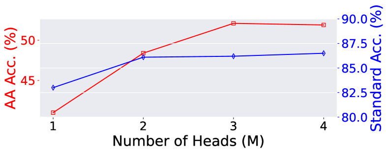
(a)

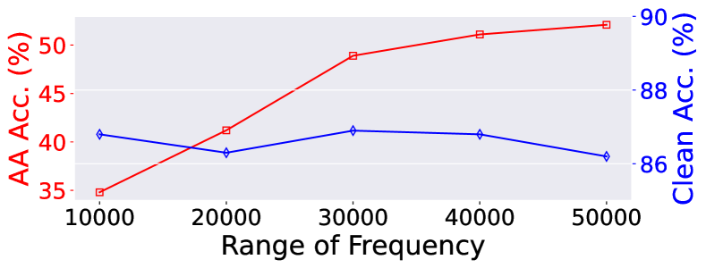
(b)

Figure 4: Sensitivity to the different number of heads and the range of frequency for PhaseAT.

5.3 Convergence of Clean and Robust Accuracy

We verify that faster learning on high-frequency information leads to better convergence for robust accuracy. To that end, we report the standard and AA accuracy during each training epoch. We use the same settings of CIFAR-10 and tabulate the results on Figure 3. Compared to the normal adversarial training (denoted as AT), PhaseAT shows faster and better convergence both on standard and robust accuracy. This indicates that the training model has smoothed predictions near the data, effectively reducing the oscillating property of predictions when adding adversarial perturbations.

5.4 Sensitivity to the Different Settings of PhaseAT

We analyze the sensitivity of PhaseAT on different settings. Since the most significant components of PhaseAT are the head and frequency, we mainly control the number of heads (i.e., $M$) and the range of frequency. Figure 4 shows how the change of each parameter affects the standard and robust accuracy on CIFAR-10. We first see that utilizing more heads leads to the improved accuracy while incurring additional computation costs. In addition, the robust accuracy is more sensitive to the different number of heads, whereas the clean accuracy does not differ significantly when more than two heads are used. When it comes to the frequency range, we observe that utilizing the wider range of the frequency leads to the improved robust accuracy. For the clean accuracy case, on the other hand, the wider range has no significant impact, which is consistent with the previous finding that low-frequency typically dominates in the real dataset [Xu et al., 2020b]. In the experiments, we use the three heads and 50k of the frequency range based on the above validation results. For the frequency range case, no further improvement was observed for more than the 50k range.

5.5 Computational Complexity

Figure 5: Comparison of the training time of each method to achieve the best robust accuracy.

We compare the training time required to achieve the best robust accuracy for each method. To fairly measure it, we use the optimized schedule in the implementations (NuAT, FBF and PGD). Figure 5 plots the comparison on CIFAR-10. The fastest defense amongst all is FBF-1 and PhaseAT shows the comparable training time. This indicates the additional time required by Fourier transform and forward-propagation to multiple heads is negligibly small. We also compare the different versions of FBF, namely FBF-2, which uses more training epochs than FBF-1 to match the training time with PhaseAT. Despite FBF’s increased accuracy (41.0 to 44.1%), PhaseAT outperforms it by a significant margin, demonstrating the efficacy of the proposed approach.

6 Related Work

6.1 Adversarial Training

One of the most effective defenses against adversarial attacks is adversarial training. Specifically, iteratively updating the attacks during training tends to show better robustness as the adversary typically performs multiple updates to generate stronger attacks [Madry et al., 2018, Zhang et al., 2019, Wu et al., 2020]. However, the adversarial robustness comes at a large computational cost and highly increased training time due to the multiple optimizations. Hence the research towards non-iterative methods has been getting attention [Wong et al., 2020, Sriramanan et al., 2020, 2021]. The common strategy is to make the FGSM-based training robust against iterative attacks. For example, [Wong et al., 2020] discover that training with FGSM-based training can be a stronger defense against iterative attacks. This FGSM can be achieved by initializing the perturbation as uniform distribution with properly adjusted perturbation and step sizes. Instead of the initialization, [Sriramanan et al., 2020] propose a non-iterative adversarial training method by introducing $L_{2}$ regularization for smoothing the loss surface initially and further reducing the weight of this term gradually over iterations for better optimization. Similarly, [Sriramanan et al., 2021] enhance the above relaxation term by involving the use of nuclear norm to generate a more reliable gradient direction by smoothing the loss surface.

6.2 F-Principle in Standard Training

The F-principle was first discovered empirically in [Rahaman et al., 2019] and [Xu et al., 2019] independently. A theoretical proof was given by [Xu et al., 2020b] only for a one-hidden layer $\tanh$ network with a mean-squared error loss function. It was later extended in [Luo et al., 2021] to multi-layer networks with general activation functions and general loss functions excluding cross-entropy loss function.

7 Conclusion

In this work, we have analyzed the behavior of adversarial training through the lens of the response frequency and have empirically observed that adversarial training causes neural networks to have slow convergence on high-frequency components. To recover such slow convergence, we first prove that F-principle still holds in adversarial training involving more generalized settings. On this basis, we propose phase-shifted adversarial training, denoted as PhaseAT, in which the model learns high-frequency contents by shifting them to low-frequency ranges. In our method, we redesign the PhaseDNN to adopt high-dimensional inputs and effectively learn adversarial data. For reliable evaluation, we carefully design adaptive attacks and evaluate the proposed method on two popular datasets, namely CIFAR-10 and ImageNet. The results clearly show that PhaseAT shows strong performance compared to other baselines, demonstrating the efficacy of faster high-frequency learning in adversarial training. While PhaseAT enables faster training on adversarial examples, the pre-processing phase to derive the first principal component can be overhead as the number of datasets increases. In future work, we will explore the way to derive the first principle component efficiently.

8 Supplementary Materials

8.1 Filtering Method for Frequency Analysis

Motivated by the examination of F-principle [Xu et al., 2020a], we use the filtering method to analyze the behavior of the neural networks in adversarial training. The idea is to split the frequency domain into two parts, i.e., low-frequency and high-frequency parts. However, the Fourier transform for high-dimensional data requires high computational costs and large memory footprints. As an alternative, we use the Fourier transform of a Gaussian function $\hat{G}$.

Let the original dataset be $\{x_{j},y_{j}\}_{j=0}^{N-1}$, and the network output for $x_{j}$ be $\mathcal{T}_{j}$. The low frequency part of the training dataset can be derived by

$$y_{j}^{low,\delta}=\frac{1}{C_{j}}\sum_{m=0}^{N-1}y_{m}G^{\delta}(x_{j}-x_{m})$$ (8.1)

where $C_{j}=\sum_{m=0}^{N-1}G^{\delta}(x_{j}-x_{m})$ is a normalization factor, and $\delta$ is the variance of the Gaussian function (we fix $\delta$ to 3). The Gaussian function can be represented as

$$G^{\delta}(x_{j}-x_{m})=\exp(-|x_{j}-x_{m}|^{2}/(2\delta)).$$ (8.2)

Then, the high-frequency part can be derived by $y_{j}^{high,\delta}\mathrel{\ensurestackMath{\stackon[1pt]{=}{\scriptstyle\Delta}}}y_{j}-y_{j}^{low,\delta}$. We also compute the frequency components for the networks, i.e, $\mathcal{T}_{j}^{low,\delta},\mathcal{T}_{j}^{high,\delta}$ by replacing $y_{j}$ with the outputs of networks, i.e., $\mathcal{T}_{j}$. Lastly, we calculate the errors to quantify the convergence in terms of low- and high-frequency.

$$e_{low}=\left(\frac{\sum_{j}\left|y_{j}^{low,\delta}-\mathcal{T}_{j}^{low,\delta}\right|^{2}}{\sum_{j}\left|y_{j}^{low,\delta}\right|^{2}}\right)^{\frac{1}{2}}$$ (8.3)

$$e_{high}=\left(\frac{\sum_{j}\left|y_{j}^{high,\delta}-\mathcal{T}_{j}^{high,\delta}\right|^{2}}{\sum_{j}\left|y_{j}^{high,\delta}\right|^{2}}\right)^{\frac{1}{2}}$$ (8.4)

8.2 Iterative-version of PhaseAT

Algorithm 2 Phase-shifted Adversarial Training (Iterative version)

1:Training epochs $T$, Dataset size $N$, PGD steps $P$, Perturbation size $\epsilon$, Perturbation step $\alpha$, Trainable networks $\mathcal{T}$, Cosine similarity function $CS(\cdot,\cdot)$

2:for $t=1$ $...$ $T$ do

3:     for $j=1$ $...$ $N$ do

4:         $\delta=$ Uniform$(-\epsilon,\epsilon)$

5:         for $k=1$ $...$ $P$ do $\triangleright$ Multiple updates of perturbations

6:              if $j$ % 2 == 0 then $\triangleright$ Alternate training on mini-batches

7:                  $\delta=\delta+\alpha\cdot$ sign($\nabla_{\delta}\ell(\mathcal{T}(x_{j}+\delta),y_{j})$)

8:              else

9:                  $\delta=\delta+\alpha\cdot$ sign($\nabla_{\delta}\ell(\mathcal{T}_{0}(x_{j}+\delta),y_{j})$)

10:              end if

11:              $\delta=$ max(min($\delta,\epsilon$), $-\epsilon$)

12:         end for

13:         $\theta=\theta-\nabla_{\theta}[\ell(\mathcal{T}(x_{j}+\delta),y_{j})$ + $CS(\mathcal{T}(x_{j}+\delta),\mathcal{T}_{0}(x_{j}+\delta)$)]

14:     end for

15:end for

For training efficiency, we design PhaseAT as a non-iterative method based on the FGSM perturbation [Wong et al., 2020]. To confirm the effect of stronger attacks in the training process of PhaseAT, we additionally introduce an iterative version of PhaseAT. Since PhaseAT is not closely related to the perturbation generation, we replace the FGSM perturbation with the perturbation generated from PGD [Madry et al., 2018]. The overall algorithm is shown in Algorithm-2.

8.3 Details about Evaluation

8.3.1 Attack Configuration

In our work, we mainly adopt the projected gradient descent (PGD) [Madry et al., 2018] and auto-attack (AA) [Croce and Hein, 2020b] to evaluate baselines. PGD is constructed by multiple updates of adversarial perturbations, and AA is the ensemble of strong attacks including the variants of PGD. Typically, AA is considered one of the strongest attacks. The details about each attack of AA are as follows:

• Auto-PGD (APGD) [Croce and Hein, 2020b]: This is parameter-free adversarial attack that adaptively changes the step size by considering the optimization of the perturbations. APGD has three variations depending on loss functions: APGD_ce, APGD_dlr, and APGD_t.

• FAB [Croce and Hein, 2020a]: This attack minimizes the norm of the perturbation necessary to achieve a misclassification. FAB has two variants, FAB and FAB_t.

• Square [Andriushchenko et al., 2020]: Compared to others, this attack belongs to the black-box attacks and is also known as score-based attack. This attack iteratively inserts an artificial square to the inputs to search optimal perturbations causing huge changes on predictions.

We set the hyper-parameter settings for each attack based on standard version of AA in robust-bench framework [Croce et al., 2021]. Note that we exclude Square attack from the AA because the stochastic process in PhaseAT can be robust against Square [Qin et al., 2021], which prevents the fair comparison with other baselines which do not include stochastic process. We thus move the results of Square attack to the Supplementary Section 8.4.2.

8.3.2 Dataset Information

We evaluate each baseline on two benchmark datasets, CIFAR-10 and ImageNet. CIFAR-10 [Krizhevsky et al., 2009] consist of 60,000 images of 32×32×3 size for 10 classes, and ImageNet contains 1.2M images of 224×224×3 size for 1,000 classes. Instead of existing ImageNet, we use the smaller version of ImageNet which used in recent baselines [Sriramanan et al., 2020, 2021], which contains 120K images of 224×224×3 size for 100 classes .

8.3.3 Baseline Setting

PhaseAT is compared to both non-iterative (FBF, GAT, and NuAT) and iterative (FBF, GAT, and NuAT) methods (PGD, TRADES, and AWP). The hyper-parameter settings of each baseline are listed in Table 6. Since the evaluation results on ImageNet come from previous works [Sriramanan et al., 2020, 2021], the table only includes the parameters reported in these works (unknown parameters are denoted with $-$.).

8.4 Additional Evaluation

8.4.1 Different Architectures

Table 4: Performance evaluation on CIFAR-10 dataset. The backbone networks are WideResNet-34-10. Best and second best results are highlighted in boldface and underline, respectively.

Method Standard accuracy PGD₅₀ AA FBF [Wong et al., 2020] 82.1 54.4 51.3 GAT [Sriramanan et al., 2020] 84.7 56.1 52.1 NuAT [Sriramanan et al., 2021] 85.1 54.6 53.4 PhaseAT (Ours.) 88.8 62.3 59.2

We conduct additional experiments by scaling the PhaseAT backbone networks to verify the effectiveness of PhaseAT on different architectures. We use WideResNet-34-10 architecture instead of PreActResNet-18 to evaluate each baseline on CIFAR-10.The comparison results are listed in Table 4. Similar to the main experiment, we see that PhaseAT achieves the best results amonst all non-iterative methods, demonstrating that PhaseAT can be well scaled to the larger networks.

8.4.2 Adversarial Robustness against Black-box Attacks

Table 5: Performance evaluation on CIFAR-10 dataset against two different black-box attacks.

Method	Standard accuracy	Transfer-based attack		Score-based attack
		VGG-11	ResNet-18
FBF [Wong et al., 2020]	84.0	80.5	80.6	53.5
GAT [Sriramanan et al., 2020]	80.5	79.8	80.3	54.1
NuAT [Sriramanan et al., 2021]	81.6	79.5	80.5	56.7
PhaseAT (Ours.)	86.2	83.8	85.0	76.5

As DNN models are often hidden from users in real-world applications, the robustness against black-box attacks is also crucial. Among the different kinds of black-box attacks, we consider transfer-based [Liu et al., 2016, Papernot et al., 2017] and score-based attacks. For transfer-based attacks, we use VGG-11 and ResNet-18 as substitute models and construct the attacks using seven steps of PGD [Madry et al., 2018]. For score-based attacks, we adopt square attack [Andriushchenko et al., 2020] with 5,000 query budgets, which is a gradient-free attack and one of the strongest attacks in black-box attacks.

Table 5 shows the robust accuracy against black-box attacks. Similar to white-box attacks, PhaseAT shows better accuracy against both transfer-based and score-based attacks in comparison to other non-iterative methods. In score-based attacks, the difference in performance between others and PhaseAT is particularly noticeable. This can be explained by the stochastic process of PhaseAT because Qin et al. [Qin et al., 2021] demonstrate that randomized defense (e.g., Gaussian noise in the inputs) can robustly prevent the model from score-based attacks. This is why we exclude square attack from the AA attack for a fair comparison with other baselines that do not include the stochastic process. Note that the stochastic property can not be circumvented in the black-box scenario because it is infeasible to design adaptive attacks (i.e., EOT attacks) as in the white-box scenario. Comprehensive results show that PhaseAT could be a robust defense strategy against both white-box and black-box attacks.

Table 6: Hyper-parameter setting for all baselines.

Method Hyper-parameters CIFAR-10 (PreActResNet-18) ImageNet-100 (ResNet-18) FBF perturbation $\epsilon$ 0.031 0.031 perturbation step size 0.039 0.039 learning rate 0.1 - epoch 30 - batch size 256 - GAT perturbation $\epsilon$ 0.031 0.031 perturbation step size 0.031 0.031 learning rate 0.1 0.1 epoch 100 100 batch size 64 64 NuAT perturbation $\epsilon$ 0.031 0.031 perturbation step size 0.031 0.031 learning rate 0.1 0.1 epoch 100 100 batch size 64 64 PGD perturbation $\epsilon$ 0.031 0.031 perturbation step size 0.039 0.039 number of iterations 7 - learning rate 0.1 - epoch 30 - batch size 256 - TRADES perturbation $\epsilon$ 0.031 0.031 perturbation step size 0.007 - beta 6.0 - learning rate 0.1 - epoch 100 - batch size 128 - PhaseDNN perturbation $\epsilon$ 0.031 0.031 perturbation step size 0.039 0.039 frequency range [0, 50000) [0, 50000) number of heads 3 3 learning rate 0.1 0.1 epoch 30 50 batch size 256 128

8.5 Proofs of Theorems 3.1 and 3.2

8.5.1 Preliminaries

Before proving Theorems 3.1 and 3.2 in this section, we start with a detailed explanation of DNNs, and then introduce the mathematical tools required for proof which can be found in standard references (e.g. [Stein and Weiss, 1971, Wolff, 2003, Muscalu and Schlag, 2013, Evans, 2010]).

Deep Neural Networks.

A DNN with $K$-hidden layers and general activation functions is a vector-valued function $\mathcal{T}_{\theta}(x):\mathbb{R}^{d}\rightarrow\mathbb{R}^{m_{K+1}}$ where $m_{k}$ denotes the number of nodes in the $k$-th layer. For $1\leq k\leq K+1$, we set ${\boldsymbol{W}}^{(k)}\in\mathbb{R}^{m_{k}\times m_{k-1}}$ and ${\boldsymbol{b}}^{(k)}\in\mathbb{R}^{m_{k}}$ as the matrices whose entries consist of the weights and biases called parameters. The parameter vector $\theta$ is then defined as

$$\theta=\big{(}\textrm{vec}({\boldsymbol{W}}^{(1)}),\textrm{vec}({\boldsymbol{b}}^{(1)}),\cdots,\textrm{vec}({\boldsymbol{W}}^{(K+1)}),\textrm{vec}({\boldsymbol{b}}^{(K+1)})\big{)}\in\mathbb{R}^{M},$$

where $M=\sum_{k=1}^{K+1}(m_{k-1}+1)m_{k}$ is the number of the parameters. Given $\theta\in\mathbb{R}^{M}$ and an activation function $\sigma:\mathbb{R}\rightarrow\mathbb{R}$, the DNN output $\mathcal{T}_{\theta}^{(K+1)}(x):\mathbb{R}^{d}\rightarrow\mathbb{R}^{m_{K+1}}$ is expressed in terms of composite functions; setting $\mathcal{T}_{\theta}^{(0)}(x)=x$, $\mathcal{T}_{\theta}^{(k)}(x):\mathbb{R}^{d}\rightarrow\mathbb{R}^{m_{k}}$ is defined recursively as

$$(\mathcal{T}_{\theta}^{(k)}(x))_{i}=\sigma\big{(}({\boldsymbol{W}}^{k}\mathcal{T}_{\theta}^{k-1}+{\boldsymbol{b}}^{k})_{i}\big{)},\,\,1\leq i\leq m_{k},\,\,1\leq k\leq K.$$

We denote the DNN output $\mathcal{T}_{\theta}^{(K+1)}(x)={\boldsymbol{W}}^{(K+1)}\mathcal{T}_{\theta}^{{(K)}}+{\boldsymbol{b}}^{(K+1)}$ by $\mathcal{T}_{\theta}(x)$.

The Basic Properties of Fourier Transforms.

Let $f\in L^{1}(\mathbb{R}^{d})$. The Fourier transform of $f$ is defined by

$$\widehat{f}(\xi)=\int_{\mathbb{R}^{d}}e^{-2\pi ix\cdot\xi}f(x)dx.$$

Then clearly

$$\|\widehat{f}\|_{L^{\infty}}\leq\|f\|_{L^{1}}.$$ (8.5)

Additionally if $\widehat{f}\in L^{1}(\mathbb{R}^{d})$, the Fourier inversion holds:

$$f(x)=\int_{\mathbb{R}^{d}}e^{2\pi ix\cdot\xi}\widehat{f}(\xi)d\xi.$$ (8.6)

If $f,g\in L^{1}(\mathbb{R}^{d})$, then $f\ast g\in L^{1}(\mathbb{R}^{d})$ and

$$\widehat{f\ast g}=\hat{f}\hat{g}.$$ (8.7)

For an $n$-tuple $\alpha=(\alpha_{1},\cdots,\alpha_{d})$ of nonnegative integers, we denote

$$D^{\alpha}=\prod_{j=1}^{d}\frac{\partial^{\alpha_{j}}}{\partial^{\alpha_{j}}_{x_{j}}}\quad\textnormal{and}\quad|\alpha|=\sum_{j=1}^{d}\alpha_{j}.$$

Then, if $D^{\alpha}f\in L^{1}(\mathbb{R}^{d})$ whenever $0\leq|\alpha|\leq s$,

$$\widehat{D^{\alpha}f}(\xi)=(2\pi i)^{|\alpha|}\xi^{\alpha}\widehat{f}(\xi).$$ (8.8)

Sobolev Spaces and Gaussian Weights.

For $s\in\mathbb{N}$, the Sobolev space $W^{s,\infty}(\mathbb{R}^{d})$ is defined as

$$W^{s,\infty}(\mathbb{R}^{d})=\{f\in L^{\infty}(\mathbb{R}^{d}):D^{\alpha}f\in L^{\infty}(\mathbb{R}^{d})\,\textnormal{for all}\,0\leq|\alpha|\leq s\}$$

equipped with the norm

$$\|f\|_{W^{s,\infty}(\mathbb{R}^{d})}=\sum_{|\alpha|\leq s}\|D^{\alpha}f\|_{L^{\infty}(\mathbb{R}^{d})}.$$

We also introduce a Gaussian weight $G_{\varepsilon}(x)=\varepsilon^{-d}e^{-\pi\varepsilon^{-2}|x|^{2}}$ for any $\varepsilon>0$ on which the Fourier transform has an explicit form,

$$\widehat{G_{\varepsilon}}(\xi)=e^{-\pi\varepsilon^{2}|\xi|^{2}}.$$ (8.9)

The final observation is that $G_{\varepsilon}$ is an approximate identity with respect to the limit $\varepsilon\rightarrow 0$ as in the following well-known lemma:

Lemma 8.1.

Let $f\in C(\mathbb{R}^{d})\cap L^{\infty}(\mathbb{R}^{d})$. Then

$$\lim_{\varepsilon\rightarrow 0}\int_{\mathbb{R}^{d}}G_{\varepsilon}(x-y)f(y)dy=f(x)$$ (8.10)

for all $x\in\mathbb{R}^{d}$.

8.5.2 Proof of Theorem 3.1

In what follows we may consider a compact domain $\Omega$ instead of $\mathbb{R}^{d}$ because the input data $\{x_{j}\}_{j=0}^{N-1}$ used for training is sampled from a bounded region.

For a discrete input data $\{x_{j}\}_{j=0}^{N-1}$, we now recall the total loss in adversarial training from Section 3.1:

$$L(\theta)=\frac{1}{N}\sum_{j=0}^{N-1}\ell(\mathcal{T}_{\theta}\circ\mathcal{A},g)(x_{j}).$$ (8.11)

From the continuity of $\mathcal{T}_{\theta}$ and $g$ in the compact domain $\Omega$, we note that $\ell(\mathcal{T}_{\theta}\circ A,g)$ is continuous and bounded for general loss functions such as mean-squared error loss and cross-entropy loss. Then we can apply Lemma 8.1 to deduce

$$L(\theta) =\lim_{\varepsilon\rightarrow 0}\frac{1}{N}\sum_{j=0}^{N-1}\int_{\mathbb{R}^{d}}G_{\varepsilon}(x_{j}-x)\ell(\mathcal{T}_{\theta}\circ\mathcal{A},g)(x)dx$$

$$=\lim_{\varepsilon\rightarrow 0}\frac{1}{N}\sum_{j=0}^{N-1}\big{(}G_{\varepsilon}\ast\ell(\mathcal{T}_{\theta}\circ\mathcal{A},g)\big{)}(x_{j}).$$ (8.12)

Using the properties $G_{\varepsilon}\in L^{1}(\mathbb{R}^{d})$ and $\ell(\mathcal{T}_{\theta}\circ\mathcal{A},g)\in L^{1}(\mathbb{R}^{d})$, we then derive from Eq. 8.7 and Eq. 8.9 that

$$G_{\varepsilon}\ast\ell(\mathcal{T}_{\theta}\circ\mathcal{A},g)\in L^{1}(\mathbb{R}^{d})$$

and

$$\savestack{\tmpbox}{\stretchto{\scaleto{\scalerel*[width("G_{\varepsilon}\ast\ell(\mathcal{T}_{\theta}\circ\mathcal{A},g)")]{\kern 0.1pt\mathchar 866\relax\kern 0.1pt}{\rule{0.0pt}{505.89pt}}}{}}{2.4ex}}\stackon[-6.9pt]{G_{\varepsilon}\ast\ell(\mathcal{T}_{\theta}\circ\mathcal{A},g)}{\tmpbox}(\xi)=e^{-\pi\varepsilon^{2}|\xi|^{2}}\,\savestack{\tmpbox}{\stretchto{\scaleto{\scalerel*[width("\ell(\mathcal{T}_{\theta}\circ\mathcal{A},g)")]{\kern 0.1pt\mathchar 866\relax\kern 0.1pt}{\rule{0.0pt}{505.89pt}}}{}}{2.4ex}}\stackon[-6.9pt]{\ell(\mathcal{T}_{\theta}\circ\mathcal{A},g)}{\tmpbox}(\xi).$$ (8.13)

Note here that by Eq. 8.5

$$\|e^{-\pi\varepsilon^{2}|\xi|^{2}}\,\savestack{\tmpbox}{\stretchto{\scaleto{\scalerel*[width("\ell(\mathcal{T}_{\theta}\circ\mathcal{A},g)")]{\kern 0.1pt\mathchar 866\relax\kern 0.1pt}{\rule{0.0pt}{505.89pt}}}{}}{2.4ex}}\stackon[-6.9pt]{\ell(\mathcal{T}_{\theta}\circ\mathcal{A},g)}{\tmpbox}(\xi)\|_{L^{1}}\leq\|\savestack{\tmpbox}{\stretchto{\scaleto{\scalerel*[width("\ell(\mathcal{T}_{\theta}\circ\mathcal{A},g)")]{\kern 0.1pt\mathchar 866\relax\kern 0.1pt}{\rule{0.0pt}{505.89pt}}}{}}{2.4ex}}\stackon[-6.9pt]{\ell(\mathcal{T}_{\theta}\circ\mathcal{A},g)}{\tmpbox}\|_{L^{\infty}}\|e^{-\pi\varepsilon^{2}|\xi|^{2}}\|_{L^{1}}\leq C\|\ell(\mathcal{T}_{\theta}\circ\mathcal{A},g)\|_{L^{1}}<\infty.$$

Hence the Fourier inversion Eq. 8.6 together with Eq. 8.13 implies

$$\big{(}G_{\varepsilon}\ast\ell(\mathcal{T}_{\theta}\circ\mathcal{A},g)\big{)}(x_{j})=\int_{\mathbb{R}^{d}}e^{2\pi ix_{j}\cdot\xi}e^{-\pi\varepsilon^{2}|\xi|^{2}}\,\savestack{\tmpbox}{\stretchto{\scaleto{\scalerel*[width("\ell(\mathcal{T}_{\theta}\circ\mathcal{A},g)")]{\kern 0.1pt\mathchar 866\relax\kern 0.1pt}{\rule{0.0pt}{505.89pt}}}{}}{2.4ex}}\stackon[-6.9pt]{\ell(\mathcal{T}_{\theta}\circ\mathcal{A},g)}{\tmpbox}(\xi)d\xi.$$ (8.14)

Substituting Eq. 8.14 into the right-hand side of Eq. 8.5.2, we immediately obtain

$$L(\theta)=\lim_{\varepsilon\rightarrow 0}\frac{1}{N}\sum_{j=0}^{N-1}\int_{\mathbb{R}^{d}}e^{2\pi ix_{j}\cdot\xi}\,e^{-\pi\varepsilon^{2}|\xi|^{2}}\savestack{\tmpbox}{\stretchto{\scaleto{\scalerel*[width("\ell\big{(}\mathcal{T}_{\theta}\circ\mathcal{A},g\big{)}")]{\kern 0.1pt\mathchar 866\relax\kern 0.1pt}{\rule{0.0pt}{505.89pt}}}{}}{2.4ex}}\stackon[-6.9pt]{\ell\big{(}\mathcal{T}_{\theta}\circ\mathcal{A},g\big{)}}{\tmpbox}(\xi)d\xi,$$ (8.15)

as desired. This completes the proof.

8.5.3 Proof of Theorem 3.2

Representing $\nabla_{\theta}L(\theta)$ in the frequency domain.

To begin with, we represent $\nabla_{\theta}L(\theta)$ in the frequency domain in the same way as in Section 8.5.2. By differentiating both sides of Eq. 8.11 with respect to $\theta$ and using Lemma 8.1, we first see

$$\nabla_{\theta}L(\theta) =\frac{1}{N}\sum_{j=0}^{N-1}\nabla_{\theta}\ell(\mathcal{T}_{\theta}\circ\mathcal{A},g)(x_{j})$$

$$=\lim_{\varepsilon\rightarrow 0}\frac{1}{N}\sum_{j=0}^{N-1}\int_{\mathbb{R}^{d}}G_{\varepsilon}(x_{j}-x)\nabla_{\theta}\ell(\mathcal{T}_{\theta}\circ\mathcal{A},g)(x)dx$$ (8.16)

if $\nabla_{\theta}\ell(\mathcal{T}_{\theta}\circ\mathcal{A},g)$ is continuous and bounded. Since $\ell(\mathcal{T}_{\theta}\circ\mathcal{A},g)$ is differentiable with respect to the first argument (as mentioned in Section 3.1) and $\mathcal{T}_{\theta}$ is differentiable with respect to $\theta$ for general activation functions such as ReLU, eLU, tanh and sigmoid, the continuity is generally permissible, and thus the boundedness follows also from compact domain. In fact, the ReLU activation function is not differentiable at the origin and neither is $\mathcal{T}_{\theta}$ on a certain union of hyperplanes; for example, when considering $1$-hidden layer neural network with $m_{1}$ nodes and $1$-dimensional output, the output is

$$\mathcal{T}_{\theta}(x)=\sum_{i=1}^{m_{1}}w_{i}^{(2)}\sigma(\boldsymbol{W}_{i}^{(1)}\cdot x+\boldsymbol{b}_{i}^{(1)}),\quad w_{i}^{(2)},b_{i}^{(1)}\in\mathbb{R},\,\boldsymbol{W}_{i}^{(1)}\in\mathbb{R}^{d}$$

and the set of non-differentiable points is a union of hyperplanes given by $\{x\in\mathbb{R}^{d}:\boldsymbol{W}_{i}^{(1)}\cdot x+\boldsymbol{b}_{i}^{(1)}=0,\,1\leq i\leq m_{1}\}$. But the $d$-dimensional volume of such thin sets is zero and thus they may be excluded from the integration region in Eq. 8.10 when applying Lemma 8.1 to obtain Eq. 8.5.3 for the case of ReLU.

Just by replacing $L(\theta)$ with $\nabla_{\theta}L(\theta)$ in the argument employed for the proof of Eq. 8.15 and repeating the same argument, it follows now that

$$\nabla_{\theta}L(\theta)=\lim_{\varepsilon\rightarrow 0}\frac{1}{N}\sum_{j=0}^{N-1}\int_{\mathbb{R}^{d}}e^{2\pi ix_{j}\cdot\xi}\,e^{-\pi\varepsilon^{2}|\xi|^{2}}\savestack{\tmpbox}{\stretchto{\scaleto{\scalerel*[width("\nabla_{\theta}\ell\big{(}\mathcal{T}_{\theta}\circ\mathcal{A},g\big{)}")]{\kern 0.1pt\mathchar 866\relax\kern 0.1pt}{\rule{0.0pt}{505.89pt}}}{}}{2.4ex}}\stackon[-6.9pt]{\nabla_{\theta}\ell\big{(}\mathcal{T}_{\theta}\circ\mathcal{A},g\big{)}}{\tmpbox}(\xi)d\xi.$$ (8.17)

We then pull $\nabla_{\theta}$ to the outside of the integration in Eq. 8.17, and recall $L_{\leq\eta}(\theta)$ and $L_{\geq\eta}(\theta)$ from Section 3.1, contributed by low and high frequencies in the loss, to see

$$\nabla_{\theta}L(\theta)\approx\nabla_{\theta}L_{\leq\eta}(\theta)+\nabla_{\theta}L_{\geq\eta}(\theta).$$ (8.18)

This approximation is more and more accurate as $\varepsilon$ diminishes smaller in Eq. 8.17, and the size of $\varepsilon$ will be later determined inversely proportional to the number of dataset $N$ or dimension $d$ to consider a natural approximation reflecting the discrete experimental setting.

Estimating $\nabla_{\theta}L_{\geq\eta}(\theta)$ in terms of $\eta$.

Now we show that for the $i$-th element of $\nabla_{\theta}L_{\geq\eta}(\theta)$

$$\Big{|}\frac{\partial L_{\geq\eta}(\theta)}{\partial\theta_{i}}\Big{|}\leq C\max(N,d^{d})\,\eta^{-2s}$$ (8.19)

which implies

$$|\nabla_{\theta}L_{\geq\eta}(\theta)|=\Big{(}\sum_{\theta}\Big{|}\frac{\partial L_{\geq\eta}(\theta)}{\partial\theta_{i}}\Big{|}^{2}\Big{)}^{1/2}\leq C\max(N,d^{d})\,\eta^{-2s}.$$

By Eq. 8.18 and this bound, we get

$$|\nabla_{\theta}L(\theta)-\nabla_{\theta}L_{\leq\eta}(\theta)|\approx|\nabla_{\theta}L_{\geq\eta}(\theta)|\leq C\max(N,d^{d})\,\eta^{-2s}$$

which completes the proof of Theorem 3.2.

To show Eq. 8.19, we first use the chain rule to calculate

$$\frac{\partial L_{\geq\eta}(\theta)}{\partial\theta_{i}}=\frac{1}{N}\sum_{j=0}^{N-1}\int_{|\xi|\geq\eta}e^{2\pi ix_{j}\cdot\xi}e^{-\pi\varepsilon^{2}|\xi|^{2}}\savestack{\tmpbox}{\stretchto{\scaleto{\scalerel*[width("\nabla_{\mathcal{T}_{\theta}}\ell(\mathcal{T}_{\theta}\circ\mathcal{A},g)\cdot\frac{\partial(\mathcal{T}_{\theta}\circ\mathcal{A})}{\partial\theta_{i}}")]{\kern 0.1pt\mathchar 866\relax\kern 0.1pt}{\rule{0.0pt}{505.89pt}}}{}}{2.4ex}}\stackon[-6.9pt]{\nabla_{\mathcal{T}_{\theta}}\ell(\mathcal{T}_{\theta}\circ\mathcal{A},g)\cdot\frac{\partial(\mathcal{T}_{\theta}\circ\mathcal{A})}{\partial\theta_{i}}}{\tmpbox}(\xi)d\xi$$

Since $\eta\leq\langle\xi\rangle:=\sqrt{1+|\xi|^{2}}$ for all $0<\eta\leq|\xi|$, we then see that for $s\in\mathbb{N}$

By a change of variables $\varepsilon\xi\rightarrow\xi$, we note

$$\|e^{-\pi\varepsilon^{2}|\xi|^{2}}\|_{L^{1}}=\varepsilon^{-d}\int_{\mathbb{R}^{d}}e^{-\pi|\xi|^{2}}d\xi\leq C\varepsilon^{-d}.$$

Hence, if we show that the $L^{\infty}$-norm in Eq. 8.5.3 is finite, then

$$\bigg{|}\frac{\partial L_{\geq\eta}(\theta)}{\partial\theta_{i}}\bigg{|}\leq C\eta^{-2s}\varepsilon^{-d}.$$

Finally, if we take $\varepsilon=\min\{1/\sqrt[d]{N},1/d\}$ for large $N,d$, we conclude

$$\bigg{|}\frac{\partial L_{\geq\eta}(\theta)}{\partial\theta_{i}}\bigg{|}\leq C\max\{N,d^{d}\}\eta^{-2s}$$ (8.20)

as desired.

Now all we have to do is to bound the $L^{\infty}$-norm in Eq. 8.5.3. Using the simple inequalities

$$\langle\xi\rangle\leq 1+|\xi|,\quad(1+|\xi|)^{M}\leq C\sum_{|\alpha|\leq M}|\xi^{\alpha}|,$$

and Eq. 8.8, Eq. 8.5 in turn, we first see

By Leibniz’s rule we then bound the $L^{1}$-norm in the above as

$$\Big{\|}D^{\alpha}\big{(}\nabla_{\mathcal{T}_{\theta}}\ell(\mathcal{T}_{\theta}\circ\mathcal{A},g)\cdot\frac{\partial(\mathcal{T}_{\theta}\circ\mathcal{A})}{\partial\theta_{i}}\big{)}\Big{\|}_{L^{1}}\leq C\sum_{|\alpha_{1}|+|\alpha_{2}|\atop=|\alpha|}\Big{\|}D^{\alpha_{1}}\nabla_{\mathcal{T}_{\theta}}\ell(\mathcal{T}_{\theta}\circ\mathcal{A},g)\cdot D^{\alpha_{2}}\frac{\partial(\mathcal{T}_{\theta}\circ\mathcal{A})}{\partial\theta_{i}}\Big{\|}_{L^{1}}.$$

When $|\alpha|\leq s-1$, $|\alpha_{1}|\leq s$ and $|\alpha_{2}|+1\leq s$, and then the $L^{1}$-norm in the right-hand side is generally finite since $\sigma\in W^{s,\infty}(\mathbb{R})$, $g\in W^{s,\infty}(\mathbb{R}^{d})$, and the $L^{1}$-norm may be taken over the compact domain $\Omega$; for example, $\ell(\mathcal{T}_{\theta}\circ\mathcal{A},g)(x)=|(\mathcal{T}_{\theta}\circ\mathcal{A})(x)-g(x)|^{2}$ and

$$\nabla_{\mathcal{T}_{\theta}}\ell(\mathcal{T}_{\theta}\circ\mathcal{A},g)(x)=2((\mathcal{T}_{\theta}\circ\mathcal{A})(x)-g(x))$$

for mean-squared error loss. Since $(\mathcal{T}_{\theta}\circ\mathcal{A})(x)$ is expressed as compositions of $\sigma$, the regularity of $\nabla_{\mathcal{T}_{\theta}}\ell(\mathcal{T}_{\theta}\circ\mathcal{A},g)(x)$ is exactly determined by that of $\sigma$ and $g$. Namely,

$$\nabla_{\mathcal{T}_{\theta}}\ell(\mathcal{T}_{\theta}\circ\mathcal{A},g)(x)\in W^{s,\infty}(\mathbb{R}^{d}),\quad(\mathcal{T}_{\theta}\circ\mathcal{A})(x)\in W^{s,\infty}(\mathbb{R}^{d}),$$ (8.21)

from which the $L^{1}$-norm taken over the compact domain $\Omega$ is finite since $|\alpha_{1}|\leq s$ and $|\alpha_{2}|+1\leq s$.

On the other hand, when $s\leq|\alpha|\leq 2s$ we set $|\alpha|=s+j$ with $0\leq j\leq s$. Firstly, if $0\leq|\alpha_{1}|\leq s$ (and so $j\leq|\alpha_{2}|\leq s+j$ since $|\alpha|=|\alpha_{1}|+|\alpha_{2}|$), then we bound

$$\Big{\|}D^{\alpha_{1}}\nabla_{\mathcal{T}_{\theta}}\ell(\mathcal{T}_{\theta}\circ\mathcal{A},g)\cdot D^{\alpha_{2}}\frac{\partial(\mathcal{T}_{\theta}\circ\mathcal{A})}{\partial\theta_{i}}\Big{\|}_{L^{1}}\leq\big{\|}D^{\alpha_{1}}\nabla_{\mathcal{T}_{\theta}}\ell(\mathcal{T}_{\theta}\circ\mathcal{A},g)\big{\|}_{L^{\infty}}\Big{\|}D^{\alpha_{2}}\frac{\partial(\mathcal{T}_{\theta}\circ\mathcal{A})}{\partial\theta_{i}}\Big{\|}_{L^{1}}.$$

Here, by Eq. 8.21, the $L^{\infty}$-norm in the right-hand side is finite since $|\alpha_{1}|\leq s$, while the finiteness of $L^{1}$-norm follows from the fact that $D^{\beta}\sigma\in L^{1}(\mathbb{R})$ where $|\beta|=|\alpha_{2}|+1$. This fact is indeed valid for general activation functions such as ReLU, eLU, tanh and sigmoid since the $L^{1}$-norm may be taken over the compact domain $\Omega$. Finally, if $s+1\leq|\alpha_{1}|\leq s+j$ (and so $0\leq|\alpha_{2}|\leq j-1$), then we bound this time

$$\Big{\|}D^{\alpha_{1}}\nabla_{\mathcal{T}_{\theta}}\ell(\mathcal{T}_{\theta}\circ\mathcal{A},g)\cdot D^{\alpha_{2}}\frac{\partial(\mathcal{T}_{\theta}\circ\mathcal{A})}{\partial\theta_{i}}\Big{\|}_{L^{1}}\leq\big{\|}D^{\alpha_{1}}\nabla_{\mathcal{T}_{\theta}}\ell(\mathcal{T}_{\theta}\circ\mathcal{A},g)\big{\|}_{L^{1}}\Big{\|}D^{\alpha_{2}}\frac{\partial(\mathcal{T}_{\theta}\circ\mathcal{A})}{\partial\theta_{i}}\Big{\|}_{L^{\infty}}.$$

Here, the $L^{\infty}$-norm in the right-hand side is finite by Eq. 8.21 since $|\alpha_{2}|+1\leq j\leq s$. The finiteness of $L^{1}$-norm also comes from $D^{\beta}\sigma\in L^{1}(\mathbb{R})$ and $D^{\beta}g\in L^{1}(\mathbb{R}^{d})$ with $s+1\leq|\beta|\leq 2s$. Here, the condition $D^{\beta}\sigma\in L^{1}(\mathbb{R})$ is valid generally as above, and the bound Eq. 8.20 is still valid with $\eta^{-s}$ even if the condition $D^{\beta}g\in L^{1}(\mathbb{R}^{d})$ is not required. This is the case $j=0$ in the proof.

References

- Andriushchenko et al. [2020] Maksym Andriushchenko, Francesco Croce, Nicolas Flammarion, and Matthias Hein. Square attack: a query-efficient black-box adversarial attack via random search. In Proc. the European Conference on Computer Vision (ECCV), 2020.
- Athalye et al. [2018] Anish Athalye, Logan Engstrom, Andrew Ilyas, and Kevin Kwok. Synthesizing robust adversarial examples. In Proc. the International Conference on Machine Learning (ICML), 2018.
- Cai et al. [2020] Wei Cai, Xiaoguang Li, and Lizuo Liu. A phase shift deep neural network for high frequency approximation and wave problems. SIAM Journal on Scientific Computing, 2020.
- Croce and Hein [2020a] Francesco Croce and Matthias Hein. Minimally distorted adversarial examples with a fast adaptive boundary attack. In Proc. the International Conference on Machine Learning (ICML), 2020a.
- Croce and Hein [2020b] Francesco Croce and Matthias Hein. Reliable evaluation of adversarial robustness with an ensemble of diverse parameter-free attacks. In Proc. the International Conference on Machine Learning (ICML), 2020b.
- Croce et al. [2021] Francesco Croce, Maksym Andriushchenko, Vikash Sehwag, Edoardo Debenedetti, Nicolas Flammarion, Mung Chiang, Prateek Mittal, and Matthias Hein. Robustbench: a standardized adversarial robustness benchmark. In Proc. the Advances in Neural Information Processing Systems (NeurIPS), 2021.
- Deng et al. [2009] Jia Deng, Wei Dong, Richard Socher, Li-Jia Li, Kai Li, and Li Fei-Fei. Imagenet: A large-scale hierarchical image database. In 2009 IEEE conference on computer vision and pattern recognition, pages 248–255. Ieee, 2009.
- Evans [2010] Lawrence C. Evans. Partial differential equations. Second edition. Graduate Studies in Mathematics. American Mathematical Society, 2010.
- Gong et al. [2021] Chengyue Gong, Tongzheng Ren, Mao Ye, and Qiang Liu. Maxup: Lightweight adversarial training with data augmentation improves neural network training. In Proc. the Conference on Computer Vision and Pattern Recognition (CVPR), 2021.
- Goodfellow et al. [2015] Ian J Goodfellow, Jonathon Shlens, and Christian Szegedy. Explaining and harnessing adversarial examples. In Proc. The International Conference on Learning Representations (ICLR), 2015.
- He et al. [2016] Kaiming He, Xiangyu Zhang, Shaoqing Ren, and Jian Sun. Deep residual learning for image recognition. In Proc. the Conference on Computer Vision and Pattern Recognition (CVPR), 2016.
- Krizhevsky et al. [2009] Alex Krizhevsky, Geoffrey Hinton, et al. Learning multiple layers of features from tiny images. 2009.
- Kurakin et al. [2016] Alexey Kurakin, Ian Goodfellow, and Samy Bengio. Adversarial machine learning at scale. In Proc. The International Conference on Learning Representations (ICLR), 2016.
- Liu et al. [2016] Yanpei Liu, Xinyun Chen, Chang Liu, and Dawn Song. Delving into transferable adversarial examples and black-box attacks. arXiv preprint arXiv:1611.02770, 2016.
- Luo et al. [2021] Tao Luo, Zheng Ma, Zhi-Qin John Xu, and Yaoyu Zhang. Theory of the frequency principle for general deep neural networks. CSIAM Transactions on Applied Mathematics, 2021.
- Madry et al. [2018] Aleksander Madry, Aleksandar Makelov, Ludwig Schmidt, Dimitris Tsipras, and Adrian Vladu. Towards deep learning models resistant to adversarial attacks. 2018.
- Muscalu and Schlag [2013] Camil Muscalu and Wilhelm Schlag. Classical and multilinear harmonic analysis. Vol. I. Cambridge Studies in Advanced Mathematics. Cambridge University Press, 2013.
- Papernot et al. [2017] Nicolas Papernot, Patrick McDaniel, Ian Goodfellow, Somesh Jha, Z Berkay Celik, and Ananthram Swami. Practical black-box attacks against machine learning. In Proceedings of the ACM on Asia conference on computer and communications security, 2017.
- Qin et al. [2019] Chongli Qin, James Martens, Sven Gowal, Dilip Krishnan, Krishnamurthy Dvijotham, Alhussein Fawzi, Soham De, Robert Stanforth, and Pushmeet Kohli. Adversarial robustness through local linearization. In Proc. the Advances in Neural Information Processing Systems (NeurIPS), 2019.
- Qin et al. [2021] Zeyu Qin, Yanbo Fan, Hongyuan Zha, and Baoyuan Wu. Random noise defense against query-based black-box attacks. In Proc. the Advances in Neural Information Processing Systems (NeurIPS), 2021.
- Rahaman et al. [2019] Nasim Rahaman, Aristide Baratin, Devansh Arpit, Felix Draxler, Min Lin, Fred Hamprecht, Yoshua Bengio, and Aaron Courville. On the spectral bias of neural networks. In Proc. the International Conference on Machine Learning (ICML), 2019.
- Rebuffi et al. [2021] Sylvestre-Alvise Rebuffi, Sven Gowal, Dan A Calian, Florian Stimberg, Olivia Wiles, and Timothy Mann. Fixing data augmentation to improve adversarial robustness. In Proc. the Advances in Neural Information Processing Systems (NeurIPS), 2021.
- Sriramanan et al. [2020] Gaurang Sriramanan, Sravanti Addepalli, Arya Baburaj, et al. Guided adversarial attack for evaluating and enhancing adversarial defenses. In Proc. the Advances in Neural Information Processing Systems (NeurIPS), 2020.
- Sriramanan et al. [2021] Gaurang Sriramanan, Sravanti Addepalli, Arya Baburaj, et al. Towards efficient and effective adversarial training. In Proc. the Advances in Neural Information Processing Systems (NeurIPS), 2021.
- Stein and Weiss [1971] Elias M. Stein and Guido Weiss. Introduction to Fourier analysis on Euclidean spaces. Princeton University Press, 1971.
- Szegedy et al. [2013] Christian Szegedy, Wojciech Zaremba, Ilya Sutskever, Joan Bruna, Dumitru Erhan, Ian Goodfellow, and Rob Fergus. Intriguing properties of neural networks. In Proc. The International Conference on Learning Representations (ICLR), 2013.
- Tramer and Boneh [2019] Florian Tramer and Dan Boneh. Adversarial training and robustness for multiple perturbations. In Proc. the Advances in Neural Information Processing Systems (NeurIPS), 2019.
- Tramèr et al. [2018] Florian Tramèr, Alexey Kurakin, Nicolas Papernot, Ian Goodfellow, Dan Boneh, and Patrick McDaniel. Ensemble adversarial training: Attacks and defenses. In Proc. The International Conference on Learning Representations (ICLR), 2018.
- Wang et al. [2021] Haotao Wang, Chaowei Xiao, Jean Kossaifi, Zhiding Yu, Anima Anandkumar, and Zhangyang Wang. Augmax: Adversarial composition of random augmentations for robust training. In Proc. the Advances in Neural Information Processing Systems (NeurIPS), 2021.
- Wolff [2003] Thomas H. Wolff. Lectures on harmonic analysis. American Mathematical Society, 2003.
- Wong et al. [2020] Eric Wong, Leslie Rice, and J Zico Kolter. Fast is better than free: Revisiting adversarial training. In Proc. The International Conference on Learning Representations (ICLR), 2020.
- Wu et al. [2020] Dongxian Wu, Shu-Tao Xia, and Yisen Wang. Adversarial weight perturbation helps robust generalization. 2020.
- Xu et al. [2019] Zhi-Qin John Xu, Yaoyu Zhang, and Yanyang Xiao. Training behavior of deep neural network in frequency domain. In International Conference on Neural Information Processing, 2019.
- Xu et al. [2020a] Zhi-Qin John Xu, Yaoyu Zhang, Tao Luo, Yan Xiao, and Zheng Ma. Frequency principle: Fourier analysis sheds light on deep neural networks. Communications in Computational Physics, 2020a.
- Xu et al. [2020b] Zhi-Qin John Xu, Yaoyu Zhang, Tao Luo, Yanyang Xiao, and Zheng Ma. Frequency principle: Fourier analysis sheds light on deep neural networks. Communications in Computational Physics, 2020b.
- Zagoruyko and Komodakis [2016] Sergey Zagoruyko and Nikos Komodakis. Wide residual networks. arXiv preprint arXiv:1605.07146, 2016.
- Zhang et al. [2019] Hongyang Zhang, Yaodong Yu, Jiantao Jiao, Eric Xing, Laurent El Ghaoui, and Michael Jordan. Theoretically principled trade-off between robustness and accuracy. In Proc. the International Conference on Machine Learning (ICML), 2019.
- Zhang et al. [2020] Jingfeng Zhang, Jianing Zhu, Gang Niu, Bo Han, Masashi Sugiyama, and Mohan Kankanhalli. Geometry-aware instance-reweighted adversarial training. In Proc. The International Conference on Learning Representations (ICLR), 2020.