Adjoint-Based Estimation of Sensitivity of Clinical Measures to Boundary Conditions for Arteries

Abstract.

The use of adjoint solvers is considered in order to obtain the sensitivity of clinical measures in aneurysms to incomplete (or unknown) boundary conditions and/or geometry. It is shown that these techniques offer interesting theoretical insights and viable computational tools to obtain these sensitivities.

1. Introduction

The analysis of haemodynamic phenomena and their clinical relevance via computational mechanics (fluids, solids, $\dots$) is now common in research and development. Yet a recurring question has been the influence of boundary conditions and geometry on ‘clinically relevant measures’. As an example, consider flows in aneurysms. A crucial question is how far upstream the geometry has to be modeled accurately in order to obtain sufficiently accurate flow predictions, as well as their associated loads on vessel walls (shear, pressures) and clinically relevant measures (such as kinetic and vortical energy, vortex line length, etc.). In many cases, users may not have sufficient upstream information, so this question is of high relevance. The thesis of Castro and subsequent publications [3, 4] have shown how dramatic the difference between well resolved upstream geometries and so-called ‘cut’ geometries can be. In some cases, completely different types of flow were seen, which in turn could have led to different clinical decisions. Figures 1-2 show two examples.

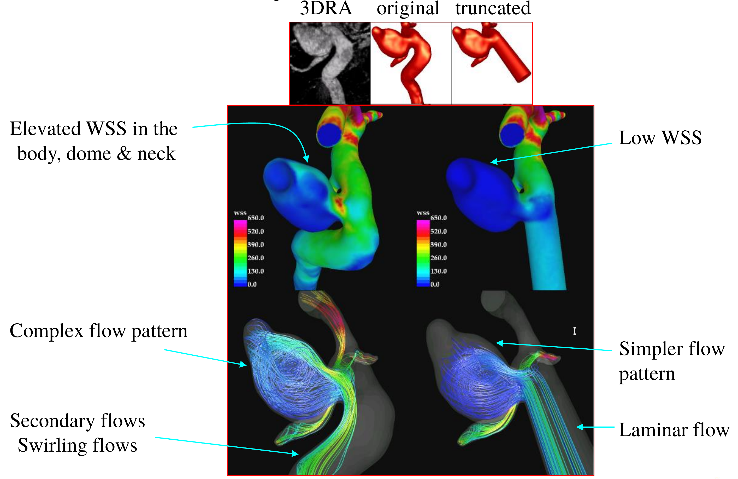
Figure 1. Vessel 1: Difference in flow features between properly resolved and unresolved upstream geometry.

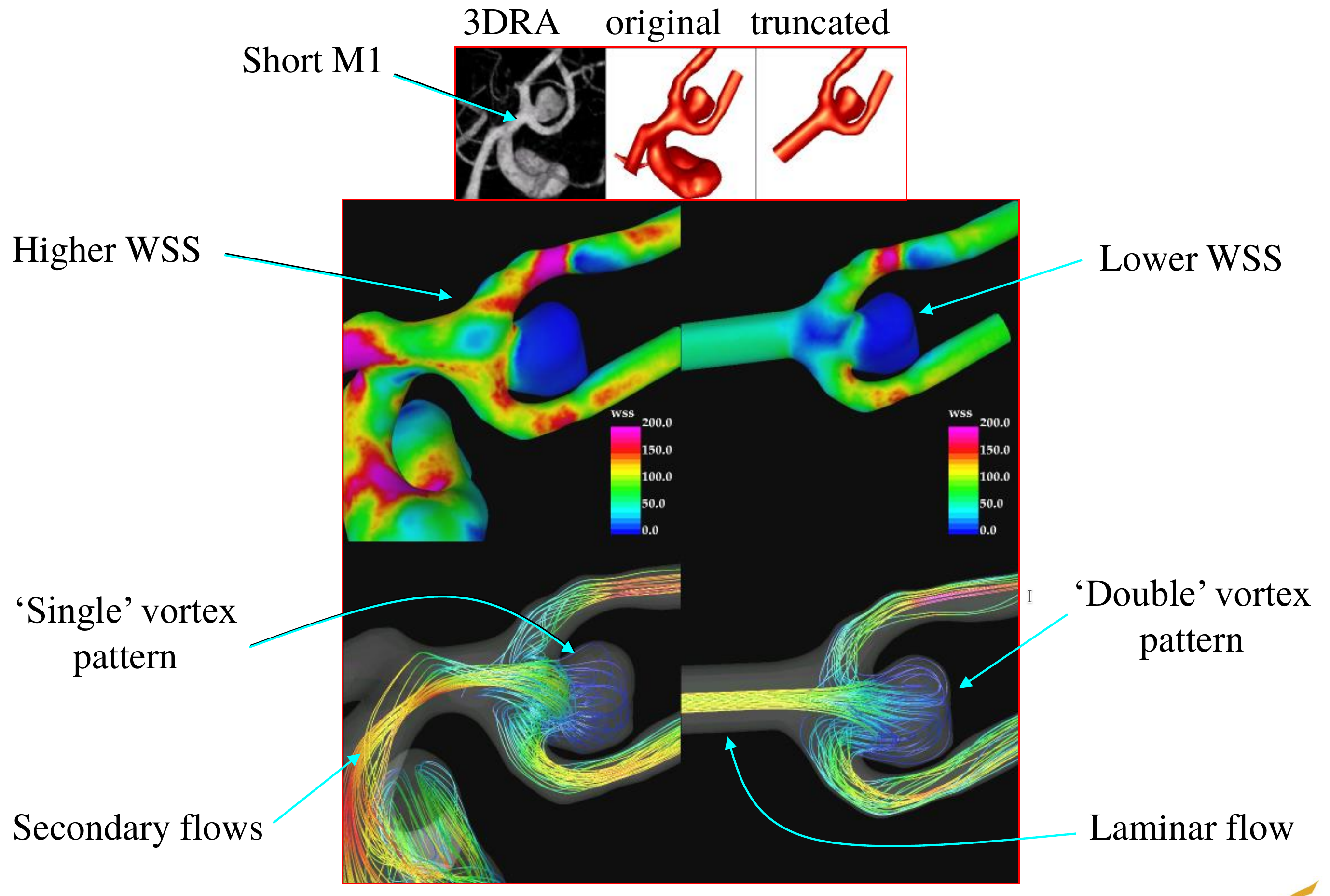
Figure 2. Vessel 2: Difference in flow features between properly resolved and unresolved upstream geometry

To complicate matters further, the flow is transient/pulsating, and the flowrate and flow profile coming in at the upstream boundary in most cases is unknown. It is a common practice to simply set some kind of pipe flow profile (Poiseuille, Womersley) at the inflow, adjusting the analytical parameters to the estimated/known flux.
The central question remains: what is the influence of a change of boundary conditions (e.g. inflow profiles) or geometry (e.g. more upstream/downstream geometry) on the clinically relevant measures ?
A simple way to answer this question is to perform several runs, each with a different geometry or different boundary condition. This finite difference approach can then yield the sensitivity of a ‘measure of clinical relevance’ $I$ to a change in geometry or boundary condition $\bm{z}$. Another possibility is via adjoints [16, 23, 13, 12, 2]. We also refer to a series of works by Glowinski and collaborators on the role of adjoints in optimization [8, 11, 21, 1, 7, 9]. See also [22, 14, 10]. We emphasize that this list is incomplete as many authors have made fundamental contributions to this topic.

1.1. Upstream Boundary Conditions for the Flow

It is known from empirical evidence and simple fluid mechanics that given any steady inflow velocity profile, after a given number of diameters along the pipe the flow will revert to a simple pipe flow (Poiseuille). This so-called hydrodynamic entry length $L_{h}$ is a function of the Reynolds number $Re$, and for laminar flow and uniform inflow is given by:

$$L_{h}=0.05Re\,D\,,\quad Re=\frac{\rho U_{e}D}{\mu}\,,$$ (1)

where $\rho,U_{e},\mu$ denote the density, mean entrance velocity and viscosity of the flow and $D$ the vessel diameter. For blood and a typical artery $\rho=1~{}g/cm^{3},U_{e}=50~{}cm/sec,\mu=0.04~{}g/cm/sec,D=0.1~{}cm$, so $Re=O(100)$ and $L_{h}=5~{}D$. Note that this estimate is only valid for steady flows and a uniform inflow. As far as the authors are aware, similar estimates for vessels with high curvatures (tortuosity) as typically encountered in arteries are not available. We note in passing that for the unsteady cases analyzed by [3, 4] the number of upstream diameters required before the flow did not change in the aneurysms was much higher than the estimate given above.

1.2. Possible Mathematical Approaches

In order to formulate the problem mathematically, we can consider different approaches.

• Empirical Data: for any given geometry/case, one could perform a series of studies, changing the type of inflow (vortical flows, unsteady flows) and seeing how long the observed hydrodynamic entry lengths are;

• Sensitivity Analysis I: one could try to obtain a ‘topological derivative’ that measures the sensitivity of the flow in the aneurysm with respect to movement of the upstream boundary.

• Sensitivity Analysis II: one could obtain a ‘flow derivative’ that measures the sensitivity of the clinical measure of the flow in the aneurysm with respect to changes of the entry flow in the upstream boundary.

Outline: The remainder of the paper is organized as follows. In Section 2, we first introduce a generic optimization problem formulation and adjoint framework. This generic discussion is well-known. This is followed by an example of Navier-Stokes specific to the aneurysm problem. We study the sensitivity with respect to the inflow velocity and inflow position. Section 3 focuses on numerical implementation. In Section 4.1, we present a specific example corresponding to the 2-D channel flow. For this example, we are able to derive explicit expressions for the state variables, adjoint variables, and the sensitivities (see Appendix A). This is followed by a realistic aneurysm example in Section 4.2, where we study the sensitivity of the ‘measure of clinical relevance’ $I$. All the numerical examples confirm the proposed approach.

2. General Adjoint Formulation

Suppose we have a ‘measure of clinical relevance’ $I$ for a region that is in or close to an aneurysm. This could be the kinetic or vortical energy, the shear stress or the length of vortex lines - all of which have been proposed in the literature [19, 5, 6].

The question then becomes: how sensitive is this measure to the (often unknown) boundary conditions imposed or the (often approximate) geometric accuracy ? Given that $I$ is a function of the unknowns $u$ and these in turn are a function of a set of parameters $z$ describing the boundary conditions or the geometry, the answer to this question is given by the gradient of $I$. Consider the well-known generic minimization problem

$$\min_{u,z}I(u,z)\quad\mbox{subject to}\quad e(u,z)=0\,,$$

where $I:U\times Z\rightarrow\mathbb{R}$ is the cost functional and $e(\cdot,\cdot):U\times Z\rightarrow Y$ is the PDE constraint. Here $U,Y$ and $Z$ are function spaces. Typically, $U,Y$ are Banach spaces and $Z$ is a Hilbert space. Under very generic conditions, one can establish existence of solution to the above optimization problems, see [12, 2]. As it has been known in the literature, there are two ways to derive the expression of the adjoint and the gradient of objective function $I$. The first approach is the so-called reduced formulation, where assuming that the PDE is uniquely solvable, one considers the well-defined control-to-state map

$$z\mapsto u(z)$$

with $(u(z),z)$ solving the PDE $e(u(z),z)=0$. The reduced objective functional is then given by $\mathcal{I}(z)=I(u(z),z)$. Then one obtains the derivative of $\mathcal{I}$ with respect to $z$ which also requires computing the sensitivites of $u$ with respect to $z$. The second approach is the full space formulation and it requires forming the Lagrangian. Under fairly generic conditions (constraint qualificiations), one can establish the existence of Lagrange multipliers in this setting, see [25, 12]. Regardless, in both cases, the same expression of gradient is obtained [2, Pg. 14].

We briefly sketch the Lagrangian approach and refer to [12, 2] for details. Let $p$ denotes the adjoint variable, then the Lagrangian functional is given by

$$L(u,z,p)=I(u,z)-\langle e(u,z),p\rangle_{Y,Y^{*}}\,.$$ (2)

Then at a stationary point $(u,z,p)$ the following conditions hold

$$L_{p}(u,z,p) =0,$$ (3)

$$L_{u}(u,z,p) =0,$$

$$L_{z}(u,z,p) =0.$$

Our goal for the application under consideration is not to solve the above optimization problem, but rather derive the expression of the gradient $L_{z}(u,z,p)$. In view of the expression of the Lagrangian given in (2), it is not difficult to see that conditions in (3) are equivalent to

$$e(u,z) =0,$$ (State equation) (4)

$$e_{u}(u,z)^{*}p =I_{u}(u,z),$$ (Adjoint equation)

$$I_{z}(u,z)-e_{z}(u,z)^{*}p =0.$$ (Gradient equation)

Namely, the gradient is given by (cf. [2, Pg. 14])

$$\nabla\mathcal{I}(z)=I_{z}(u,z)-e_{z}(u,z)^{*}p.$$ (5)

The consequences of the above formulation are profound:

• The variation of $I$ in (5) exhibits only derivatives with respect to $z$, i.e., no explicit derivatives with respect to $u$ appear;

• The cost of evaluation of gradients is independent of the number of design variables (!).

In the next section, we will apply this abstract framework to the case where the PDE $e(u,z)=0$ is given by the incompressible Navier-Stokes equations. These equations are used to model the flow in the aneurysms.

2.1. Incompressible Navier-Stokes and Sensitivity with Respect to Inflow

Let the domain $\Omega\subset\mathbb{R}^{d}$ be sufficiently smooth, and consisting of two subdomains $\Omega_{\rm aneurysm}$ and the remainder of the domain $\Omega\setminus\Omega_{\rm aneurysm}$ consisting of vascular vessels. Furthermore, let the boundary $\Gamma$ of $\Omega$ consist of three parts $\Gamma_{\rm in}$ (inflow), $\Gamma_{\rm fixed}$ (fixed / wall), and $\Gamma_{\rm out}$ (outflow). Moreover, let $(\bm{u},p)$ denote the velocity-pressure pair solving the incompressible Navier-Stokes equations:

$$\begin{aligned} -\mbox{div}(\mu\nabla\bm{u})+(\bm{u}\cdot\nabla)\bm{u}+\nabla p&=\bm{f}\quad\mbox{in }\Omega\\ \mbox{div }\bm{u}&=0\quad\mbox{in }\Omega\\ \bm{u}&=\bm{z}\quad\mbox{on }\Gamma_{\rm in}\\ \bm{u}&=\bm{0}\quad\mbox{on }\Gamma_{\rm fixed}\\ (\mu\nabla\bm{u}-pI)\cdot\bm{n}&=\bm{0}\quad\mbox{on }\Gamma_{\rm out}\end{aligned}$$ (6)

where $\bm{f}$ denotes a given force (for the current set of applications $\bm{f}=0$), $\mu$ is viscosity, and $\bm{n}$ is the outward unit normal. Finally, $\bm{z}$ is some given velocity profile on the inflow boundary $\Gamma_{\rm in}$.

Given a quantity of interest (measure of clinical relevance), $I(\bm{u},p,\bm{z})$, the goal is to obtain the derivative of $I$ with respect $\bm{z}$ with the help of adjoint formulation as discussed in the previous section. We begin by stating the following result, see [24, Appendix C]

Lemma 1.

Let $\bm{u}$, $\bm{v}$ and $\tilde{\bm{u}}$ be smooth vector fields, then

$$\int_{\Omega}[(\bm{u}\cdot\nabla)\bm{v}]\tilde{\bm{u}}=-\int_{\Omega}(\mbox{div }\bm{u})(\bm{v}\cdot\tilde{\bm{u}})+[(\bm{u}\cdot\nabla)\tilde{\bm{u}}]\cdot\bm{v}+\int_{\Gamma}(\bm{u}\cdot\bm{n})(\bm{v}\cdot\tilde{\bm{u}}).$$

When $\bm{v}=\bm{u}$ and div $\bm{u}=0$, then

$$\int_{\Omega}[(\bm{u}\cdot\nabla)\bm{u}]\tilde{\bm{u}}=-\int_{\Omega}[(\bm{u}\cdot\nabla)\tilde{\bm{u}}]\cdot\bm{u}+\int_{\Gamma}(\bm{u}\cdot\bm{n})(\bm{u}\cdot\tilde{\bm{u}}).$$

Next, a derivation of sensitivity is provided using the adjoint approach. We begin by writing the Lagrangian functional

$$L(\bm{u},p,\tilde{\bm{u}},\tilde{p},\tilde{\bm{u}}_{\Gamma}) =I(\bm{u},p,\bm{z})-\left[\int_{\Omega}\left(-\mbox{div}(\mu\nabla\bm{u})+(\bm{u}\cdot\nabla)\bm{u}+\nabla p-\bm{f}\right)\cdot\tilde{\bm{u}}-\tilde{p}\mbox{div }\bm{u}\,{\rm dx}\right.$$

$$\quad\left.+\int_{\Gamma_{\rm in}}(\bm{u}-\bm{z})\cdot\tilde{\bm{u}}_{\Gamma}\,{\rm ds}\right].$$

Applying integration-by-parts, and using Lemma 1, along with $\bm{u}=0$ on $\Gamma_{\rm fixed}$ and $(\mu\nabla\bm{u}-pI)\bm{n}=0$ on $\Gamma_{\rm out}$, we obtain that

$$L(\bm{u},p,\tilde{\bm{u}},\tilde{p},\tilde{\bm{u}}_{\Gamma}) =I(\bm{u},p,\bm{z})-\left[\int_{\Omega}\mu\nabla\bm{u}:\nabla\tilde{\bm{u}}-[(\bm{u}\cdot\nabla)\tilde{\bm{u}}]\cdot\bm{u}-p\mbox{div }\tilde{\bm{u}}+\bm{u}\cdot\nabla\tilde{p}\,{\rm dx}\right.$$

$$\quad+\int_{\Gamma_{\rm in}\cup\Gamma_{\rm fixed}}\tilde{\bm{u}}\cdot\left(-\mu\nabla\bm{u}+pI\right)\bm{n}\,{\rm ds}-\int_{\Gamma_{\rm in}\cup\Gamma_{\rm out}}\bm{u}\cdot\bm{n}\tilde{p}\,{\rm ds}$$

$$\quad\left.+\int_{\Gamma_{\rm in}}(\bm{u}-\bm{z})\cdot\tilde{\bm{u}}_{\Gamma}\,{\rm ds}+\int_{\Gamma_{\rm in}\cup\Gamma_{\rm out}}(\bm{u}\cdot\bm{n})(\bm{u}\cdot\tilde{\bm{u}}){\rm ds}\right].$$

Applying integration-by-parts again, we arrive at

$$\begin{aligned} L(\bm{u},p,\tilde{\bm{u}},\tilde{p},\tilde{\bm{u}}_{\Gamma})&=I(\bm{u},p,\bm{z})-\left[\int_{\Omega}\left(-\mbox{div}(\mu\nabla\tilde{\bm{u}})+\nabla\tilde{p}\right)\cdot\bm{u}-[(\bm{u}\cdot\nabla)\tilde{\bm{u}}]\cdot\bm{u}-p\mbox{div }\tilde{\bm{u}}\,{\rm dx}\right.\\ &\quad+\int_{\Gamma_{\rm in}\cup\Gamma_{\rm fixed}}\tilde{\bm{u}}\cdot\left(-\mu\nabla\bm{u}+pI\right)\bm{n}\,{\rm ds}+\int_{\Gamma_{\rm in}}\bm{u}\cdot(\mu\nabla\tilde{\bm{u}}-\tilde{p}I)\bm{n}\,{\rm ds}\\ &\quad+\int_{\Gamma_{\rm out}}\bm{u}\cdot(\mu\nabla\tilde{\bm{u}}-\tilde{p}I)\bm{n}\,{\rm ds}\\ &\quad+\left.\int_{\Gamma_{\rm in}}(\bm{u}-\bm{z})\cdot\tilde{\bm{u}}_{\Gamma}\,{\rm ds}+\int_{\Gamma_{\rm in}\cup\Gamma_{\rm out}}(\bm{u}\cdot\bm{n})(\bm{u}\cdot\tilde{\bm{u}}){\rm ds}\right].\end{aligned}$$ (7)

In view of (3), taking a variation of $L$ with respect to $(\bm{u},p)$ and setting it equal to zero, we obtain the adjoint equation

$$-\mbox{div}(\mu\nabla\tilde{\bm{u}})-(\bm{u}\cdot\nabla)\tilde{\bm{u}}-(\nabla\tilde{\bm{u}})^{\top}\bm{u}+\nabla\tilde{p} =I_{\bm{u}}(\bm{u},p,\bm{z})\quad\mbox{in }\Omega$$ (8)

$$\mbox{div }\tilde{\bm{u}} =-I_{p}(\bm{u},p,\bm{z})\quad\mbox{in }\Omega$$

$$\tilde{\bm{u}} =\bm{0}\quad\mbox{on }\Gamma_{\rm in}\cup\Gamma_{\rm fixed}$$

$$(\mu\nabla\tilde{\bm{u}}-\tilde{p}I)\bm{n} =-\left[(\bm{u}\cdot\tilde{\bm{u}})\bm{n}+(\bm{u}\cdot\bm{n})\tilde{\bm{u}}\right]\quad\mbox{on }\Gamma_{\rm out}.$$

We note the compatibility condition:

$$\tilde{\bm{u}}_{\Gamma}=-(\mu\nabla\tilde{\bm{u}}-\tilde{p}I)\bm{n}-(\bm{u}\cdot\tilde{\bm{u}})\bm{n}-(\bm{u}\cdot\bm{n})\tilde{\bm{u}}=-(\mu\nabla\tilde{\bm{u}}-\tilde{p}I)\bm{n}\quad\mbox{on }\Gamma_{\rm in},$$

where in the last equality we used the fact that $\tilde{\bm{u}}=\bm{0}$ on $\Gamma_{\rm in}$. We notice that, if $I$ is independent of $p$, then we obtain the standard incompressibility condition for $\tilde{\bm{u}}$ in (8). Finally, the required variation of $I$ with respect to $\bm{z}$ is given by

$$D_{\bm{z}}I(\bm{u},p,\bm{z}) =I_{\bm{z}}(\bm{u},p,\bm{z})-\left[(\mu\nabla\tilde{\bm{u}}-\tilde{p}I)\bm{n}+(\bm{u}\cdot\tilde{\bm{u}})\bm{n}+(\bm{u}\cdot\bm{n})\tilde{\bm{u}}\right]\quad\mbox{on }\Gamma_{\rm in}$$ (9)

$$=I_{\bm{z}}(\bm{u},p,\bm{z})-\left[(\mu\nabla\tilde{\bm{u}}-\tilde{p}I)\bm{n}\right]\quad\mbox{on }\Gamma_{\rm in}\,,$$

where we have again used the fact that $\tilde{\bm{u}}=\bm{0}$ on $\Gamma_{\rm in}$. Note that if the clinical measure $I$ is not a function of the control variable (in this case the inflow velocity), for a channel with constant flow in the normal direction $\bm{n}$ (i.e. $\mu\nabla\tilde{\bm{u}}\cdot\bm{n}=0$) the sensitivity reverts to (recall that $\mathcal{I}$ is the reduced objective)

$$D_{\bm{z}}\mathcal{I}(\bm{z})=\tilde{p}\bm{n}\quad\mbox{on }\Gamma_{\rm in}\,.$$ (10)

i.e. the sensitivity to inflow velocities is the adjoint pressure.

2.1.1. Sensitivity to Changes in Inflow Position

Consider next the variation of the Lagrangian $L$ given in (7) with respect to the normal $\bm{n}$. We recall that after simplifications, we have

$$L(\bm{u},p,\tilde{\bm{u}},\tilde{p},\tilde{\bm{u}}_{\Gamma})=I(\bm{u},p,\bm{z})-\int_{\Gamma_{\rm in}}(\bm{u}-\bm{z})\left[(\mu\nabla\tilde{\bm{u}}-\tilde{p}I)\bm{n}\right]\,.$$

Then

$$D_{\bm{n}}L(\bm{u},p,\tilde{\bm{u}},\tilde{p},\tilde{\bm{u}}_{\Gamma})\bm{h} =D_{\bm{n}}I(\bm{u},p,\bm{z})\bm{h}-\int_{\Gamma_{\rm in}}D_{\bm{n}}\left[(\bm{u}-\bm{z})\left((\mu\nabla\tilde{\bm{u}}-\tilde{p}I)\bm{n}\right)\right]\bm{h}$$

$$=D_{\bm{n}}I(\bm{u},p,\bm{z})\bm{h}$$

$$\quad-\int_{\Gamma_{\rm in}}(D_{\bm{n}}\bm{u}\bm{h})\left[\left((\mu\nabla\tilde{\bm{u}}-\tilde{p}I)\bm{n}\right)\right]+(\bm{u}-\bm{z})D_{\bm{n}}\left[\left((\mu\nabla\tilde{\bm{u}}-\tilde{p}I)\bm{n}\right)\right]\bm{h}$$

$$=D_{\bm{n}}I(\bm{u},p,\bm{z})\bm{h}-\int_{\Gamma_{\rm in}}(D_{\bm{n}}\bm{u}\bm{h})\left[\left((\mu\nabla\tilde{\bm{u}}-\tilde{p}I)\bm{n}\right)\right]\,,$$

where, in the last step, we have used the fact that $\bm{u}=\bm{z}$ on $\Gamma_{\rm in}$. In case, $I$ is independent of $\bm{n}$, we then obtain that

$$D_{\bm{n}}L(\bm{u},p,\tilde{\bm{u}},\tilde{p},\tilde{\bm{u}}_{\Gamma})\bm{h}=-\int_{\Gamma_{\rm in}}(D_{\bm{n}}\bm{u}\bm{h})\left[\left((\mu\nabla\tilde{\bm{u}}-\tilde{p}I)\bm{n}\right)\right]\,.$$

Note that if $\mu\nabla\tilde{\bm{u}}\cdot\bm{n}=0$ (as is often the case) the sensitivity reverts to (recall that $\mathcal{I}$ is the reduced objective)

$$D_{\bm{n}}\mathcal{I}(\bm{n})=u^{n}_{n}\tilde{p}\quad\mbox{on }\Gamma_{\rm in}$$ (11)

i.e. the sensitivity to changes in inflow position is the adjoint pressure multiplied by the normal derivative of the inflow velocity.

2.2. In- and Outflow Boundary Conditions for the Adjoint

Consider the aneurysm shown in Figure 3.

Figure 3. Schematic of Aneurysm

For the usual (forward) incompressible Navier-Stokes calculation, one would prescribe a velocity profile ($\bm{u}=\bm{z}$) at the inflow boundary and the ‘do nothing’ ($(\eta\nabla\bm{u}-pI)\bm{n}=0$) or pressure boundary condition ($p=p_{ou}$) at the outflow boundary. This implies letting the pressure ‘free’ at the inflow and the velocity ‘free’ at the outflow. At the walls the velocity is zero, i.e. $\bm{u}|_{\Gamma_{\rm fixed}}=\bm{0}$. Consider now the adjoint problem. The boundary conditions in this case are described in (8), i.e., we obtain zero velocity at the inflow and ‘do nothing’ or prescribed zero adjoint pressure at the outflow. The adjoint velocity is also zero on the walls.

3. Numerical Implementation

In a strict mathematical sense, the adjoint solver obtained by discretizing the adjoint partial differential equation should be as close as possible to the discrete adjoint obtained from transposing and manipulating the discretization of the forward problem. In this way ‘optimize-then-discretize’ and ’discretize-then-optimize’ are as close as possible. This was not adopted in the present case. Instead, while the forward problem was solved for the incompressible Navier-Stokes equations, the adjoint equations were derived for the quasi-incompressible Navier-Stokes equations, which for steady flows give the same results. Furthermore, while the forward problem was integrated to steady state using a fractional step solver with implicit solution of the viscous terms and the pressure increments, and edge-based upwinding for the velocities and 4th order pressure stabilization [17], the adjoint was discretized in space using the following scheme, which for each point $i$ in the mesh is given by:

$$\left[{\bf A}^{k}\right]^{T}_{i}M_{i}\nabla^{k}(\tilde{\bm{u}})_{i}+{\bf B}^{T}(\mu_{i}+\mu_{j})K_{ij}({\tilde{\bm{u}}}_{i}-{\tilde{\bm{u}}}_{j})+M_{i}I^{\Omega}_{\bm{u}}+D_{i}=0\,,$$

where ${\bf A},M_{i},\nabla^{k},K_{ij},D_{i}$ denote the Jacobians of the advective fluxes, lumped mass-matrix, discrete gradient in direction $k$, Laplacian edge-based coefficients and damping vector, and

$$\nabla^{k}(\tilde{\bm{u}})_{i}=C^{k}_{ij}({\tilde{\bm{u}}}_{i}+{\tilde{\bm{u}}}_{j})\,,$$

where $C^{k}_{ij}$ are the edge-based coefficients for the gradient (see [17], Chapter 20). Furthermore

$$D_{i}=-\lambda^{(ij)}\left[\tilde{\bm{u}}_{i}-\tilde{\bm{u}}_{j}+{\beta\over 2}{\bf l}_{ij}\cdot(\nabla(\tilde{\bm{u}})_{i}+\nabla(\tilde{\bm{u}})_{j})\right]\,,$$

where $c$ is the speed of sound, $\tilde{p}$ the adjoint pressure, $\lambda=|\bm{u}|+c$ the maximum eigenvalue of the system and $0<\beta<1$ denotes a pressure sensor function of the form [20].

$$\beta=1-{{\tilde{p}_{i}-\tilde{p}_{j}+0.5{\bf l}_{ij}\cdot(\nabla(\tilde{p})_{i}+\nabla(\tilde{p})_{j})|}\over{|\tilde{p}_{i}-\tilde{p}_{j}|+|0.5{\bf l}_{ij}\cdot(\nabla(\tilde{p})_{i}+\nabla(\tilde{p})_{j})|}}~{}~{}.$$

For $\beta=0,1$, second and fourth order damping operators are obtained respectively. Several other forms are possible for the sensor function $\beta$ [18].

Although this discretization of the adjoint Euler fluxes looks like a blend of second and fourth order dissipation, it has no adjustable parameters. Defining $\bm{U}=(\bm{u},p)$, $\tilde{\bm{U}}=(\tilde{\bm{u}},\tilde{p})$ Eqn.(**) may be re-written as

$${\bf R}(\bm{U},\tilde{\bm{U}})=0\,,$$

the system re-written as an unsteady equation of the form:

$$\tilde{\bm{U}}_{,\tau}+{\bf R}(\bm{U},\tilde{\bm{U}})=0\,,$$

and integrated in pseudo-time $\tau$ via a classic explicit multistep Runge-Kutta [15].

4. Numerical Examples

We will focus on two main examples. At first, we consider Poisuille flow through a channel in Section 4.1. Remarkably enough, we are able to derive the explicit expressions for all the quantities, such as solution to the state equation, adjoint equation and sensitivities, see Appendix A. These theoretical results are also confirmed by numerical results. In Section 4.2, we focus on a realistic aneurysm scenario, where we truly see the benefits of the proposed sensitivity approach.

4.1. Poiseuille Flow

The 2-D channel flow provides a good test to verify the implementation of the forward and adjoint solvers. The domain considered is of dimension $0.0\leq x\leq 0.5$, $-0.05\leq y\leq 0.05$ and $-0.005\leq z\leq 0.005$. A parabolic inflow with maximum velocity of $u_{max}=1.0$ was prescribed. The velocity at the top and bottom walls ($y_{min},y_{max}$) was prescribed to zero, and the velocity in the $z$-direction was prescribed to zero for the back and front walls ($z_{min},z_{max}$). The other relevant parameter is $\mu=0.01$. Two ‘clinically relevant measures’ (i.e. cost functions) were considered: kinetic energy $I=\frac{1}{2}\int_{\Omega}\rho{\bm{u}}^{2}\mbox{ dx}$ and vortical energy $I=\frac{1}{2}\int_{\Omega}\rho|\nabla\times\bm{u}|^{2}\mbox{ dx}$. We set $\rho=1.0$ in our experiments. The derivation of the exact solutions for the adjoint equations for these cost functions may be found in Appendix A. Let $\bm{u}=(u,v,w)^{\top}$, then the $x$-component of $\bm{u}$ is given by:

$$u=\left[1-{4\over H^{2}}y^{2}\right]u_{0}\,,$$

where $u_{0}=u_{max}$ and $H$ is the total height of the channel, i.e. $y_{max}=-y_{min}=H/2$. We thus obtain

$$\partial_{y}u=-{{8u_{0}}\over H^{2}}y,\quad\partial_{yy}u=-{{8u_{0}}\over H^{2}},\quad\partial_{x}p=-{{8\mu u_{0}}\over H^{2}}.$$

The pressure, velocity magnitude, and velocity vectors are shown in Figures 4-6.

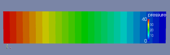
Figure 4. Poiseuille Flow: Pressure

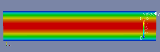
Figure 5. Poiseuille Flow: Velocity Magnitude

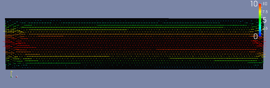
Figure 6. Poiseuille Flow: Velocity

4.1.1. Kinetic Energy

Consider the cost function

$$I=\frac{1}{2}\int\rho|\bm{u}|^{2}\mbox{ dx}\,,$$

implying

$$I_{u}=\rho u.$$

As can be seen in Appendix 1, the adjoint pressure for this cost function is:

$$\partial_{x}\tilde{p}={4\over 5}\rho u_{0}~{}~{},$$

i.e. the gradient of the adjoint pressure is also constant and linearly dependent of $u_{0}$. The results obtained are shown in Figures 7-9.

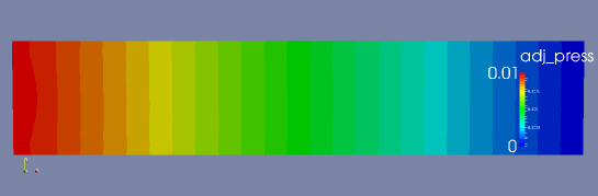
Figure 7. Poiseuille Flow: Adjoint Pressure

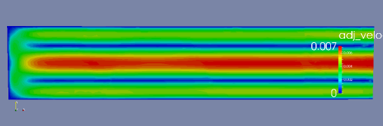
Figure 8. Poiseuille Flow: Magnitude of Adjoint Velocity. Here the cost function is Kinetic Energy.

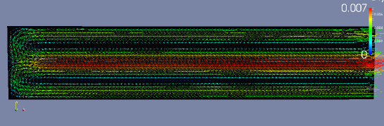
Figure 9. Poiseuille Flow: Adjoint Velocity. Here the cost function is Kinetic Energy.

4.1.2. Vortical Energy

The cost function is given by

$$I={1\over 2}\int\rho\left|\nabla\times\bm{u}\right|^{2}d\Omega~{}~{}.$$

For the 2-D channel ($u=u(y),v=0,w=z$)

$$(\nabla\times\bm{u})^{2}=\left(\partial_{y}u\right)^{2}~{}~{},$$

so that

$$I_{,u}=\rho u_{,y}(u_{,y})_{,u}=-\rho u_{,yy}=-{\rho\over\mu}p_{,x}~{}~{}={{8\rho u_{0}}\over H^{2}}~{}~{},$$

i.e. constant. As can be seen in Appendix 1, the adjoint velocities and pressure are given by:

$$\tilde{u}(x,y)=0~{}~{},~{}~{}\tilde{v}(x,y)=0~{}~{},-\tilde{p}={\rho\over\mu}p~{}~{}.$$

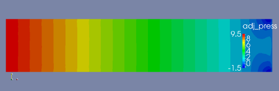
Figure 10. Poiseuille Flow: Adjoint Pressure. Cost Function: Vortical Energy.

4.2. Aneurysm with Simple Flow Pattern

As an example, we include an aneurysm with simple flow pattern. The geometry and discretization may be discerned from Figures 11a-c which show the surface triangulation, pressure and magnitude of the velocity. The region for the source-terms of the adjoint is shown in Figure 12 a and the adjoint pressure, as well as the magnitude of the adjoint velocities obtained in Figures 12 b,c. The adjoint velocites can also be seen in Figures 13 a,b. Note the effect of the source-term that pushes the adjoint flow and forms a double vortex.

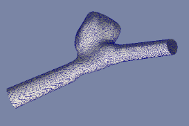
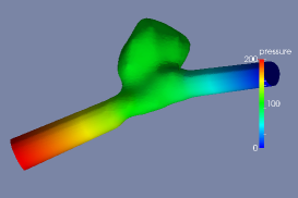
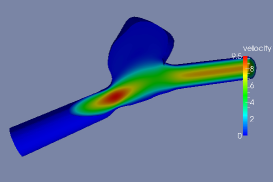
Figure 11. a,b,c  Aneurysm: Surface Triangulation, Surface Pressure and Magnitude of Velocity in Cut Plane

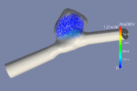
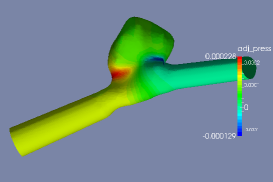
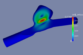
Figure 12. a,b,c  Aneurysm: Source, Adjoint Pressure and Magnitude of Adjoint Velocity in Cut Plane

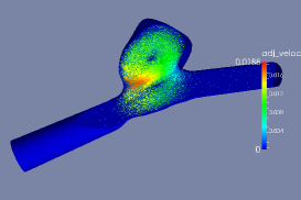
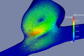
Figure 13. a,b  Aneurysm: Adjoint Velocity in Cut Plane

5. Conclusions and Outlook

The use of adjoint solvers to assess the sensitivity of incomplete boundary (inflow, geometry) information has been considered. The results of this investigation indicate that the sensitivity of clinical measures or other flow features that are inside the flow domain with respect to inflow velocity is proportional to the adjoint pressure, while the sensitivity with respect to inflow geometry is given by the product of the adjoint pressure and the normal derivative of the inflow velocity. Thus, the adjoint pressure may be a good indicator to see if the inflow boundary of haemodynamic cases is far enough from the region of interest so that errors can be avoided. The use of adjoint solvers is not unproblematic. Unlike running a series of cases, varying inflow profiles and geometry, and seeing their influence on many clinically relevant measures, adjoints require a different run for each of the clinical measures.

Appendix A Appendix 1: Analytical Expressions for Poiseuille Flow

A.1. Exact Forward Solution

Let us consider a long 2-D channel of length $0\leq x\leq L$ and width $-H/2\leq y\leq H/2$ with incompressible viscous flow. Let $\bm{u}=(u,v,w)^{\top}$, then the equation for the $x$-velocity $u$ is given by:

$$u\partial_{x}u+v\partial_{y}u+\partial_{x}p=\mu\Delta u\,.$$

Assuming a constant velocity profile in $x$, i.e. $u=u(y)$ and laminar flow with $v=0$, the solution is the Poiseuille solution, given by:

$$u=\left[1-{4\over H^{2}}y^{2}\right]u_{0}\,,$$ (12)

where $u_{0}$ is the maximum velocity at the center of the channel, and the channel extends in height from $-H/2\leq y\leq H/2$, implying

$$\partial_{y}u=-{{8u_{0}}\over H^{2}}y\,,$$

and

$$\partial_{yy}u=-{{8u_{0}}\over H^{2}}\,,$$

so that the constant pressure gradient is given by:

$$\partial_{x}p=-{{8\mu u_{0}}\over H^{2}}\,,$$

where we have used the fact that $\partial_{x}u=\partial_{xx}u=0$. The average velocity is then:

$${\overline{u}}={1\over H}\int_{-H/2}^{H/2}u\mbox{ dy}={2\over 3}u_{0}\,.$$

A.2. Adjoint Equations

The equation for the adjoint $x$-velocity $\tilde{u}$ is given by:

$$-u\partial_{x}\tilde{u}-v\partial_{y}\tilde{u}+\partial_{x}\tilde{p}=\mu\Delta\tilde{u}_{,xx}+I_{u}$$

Here $I$ is the cost function. For the channel $u$ is given by (12) and $v=0$.

Kinetic Energy: If the cost function is given by the kinetic energy

$$I={1\over 2}\int\rho|\bm{u}|^{2}\mbox{ dx}\,,$$

then

$$I_{u}=\rho u\,.$$

Assuming a long channel with no change in $x$ of the variables, the equation for the adjoint $x$-velocity $\tilde{u}$ simplifies to:

$$\partial_{x}\tilde{p}=\mu\partial_{yy}\tilde{u}+\rho u_{0}\left[1-{4\over H^{2}}y^{2}\right]\,.$$

Assuming furthermore that $\partial_{x}\tilde{p}$ is constant, and applying the boundary conditions $\tilde{u}=0$ for $y=-H/2$ and $y=H/2$ this yields

$$\tilde{u}={1\over{2\mu}}\left[-\partial_{x}\tilde{p}+\rho u_{0}\right]\left[{H^{2}\over 4}-y^{2}\right]-{{\rho u_{0}}\over{3\mu H^{2}}}\left[{H^{4}\over{16}}-y^{4}\right].$$

If we consider that at the inflow boundary $\tilde{u}=0$, then as the adjoint velocity field is also divergence-free, in any section of $x$ we must have:

$$\int\tilde{u}dy=0.$$

This implies:

$$\int_{-H/2}^{H/2}\tilde{u}\mbox{ dy}={1\over{2\mu}}\left[-\partial_{x}\tilde{p}+\rho u_{0}\right]\left[{H^{2}\over 4}y-{y^{3}\over 3}\right]_{-H/2}^{H/2}-{{\rho u_{0}}\over{3\mu H^{2}}}\left[{H^{4}\over{16}}y-{y^{5}\over 5}\right]_{-H/2}^{H/2}=0.$$

Evaluation of all terms leads to the remarkable result:

$$\partial_{x}\tilde{p}={4\over 5}\rho u_{0}=-{{\rho H^{2}}\over{10\mu}}\partial_{x}p\,,$$

i.e. the gradient of the adjoint pressure is also constant and linearly dependent of $u_{0}$. Given that the base level of the pressure $p$ is arbitrary, we might set it so that it vanishes at the exit, i.e. $p=0$. We finally obtain the remarkable result that:

$$-\tilde{p}={{\rho H^{2}}\over{10\mu}}p\,,$$

i.e. the pressure and adjoint pressure are related by the factor ${{\rho H^{2}}\over{10\mu}}$ and have a constant gradient in the field. The adjoint velocity is given by:

$$\tilde{u}={{\rho u_{0}}\over{\mu}}\left\{{1\over{10}}\left[{H^{2}\over 4}-y^{2}\right]-{1\over{3H^{2}}}\left[{H^{4}\over{16}}-y^{4}\right]\right\}\,.$$

At the center of the channel the velocity is given by:

$$\tilde{u}(y=0)={{\rho u_{0}H^{2}}\over{240\mu}}\,.$$

Vortical Energy: If the cost function is given by the vortical energy

$$I={1\over 2}\int\rho\left|\nabla\times\bm{u}\right|^{2}\mbox{ dx}\,,$$

then, for the 2-D channel ($u=u(y),v=0,w=z$)

$$|\nabla\times\bm{u}|^{2}=\left(\partial_{y}u\right)^{2}~{}~{},$$

so that

$$I_{u}=\rho\partial_{y}u(\partial_{y}u)_{,u}=-\rho\partial_{yy}u=-{\rho\over\mu}\partial_{x}p={{8\rho u_{0}}\over H^{2}}\,,$$

i.e. constant (!). Assuming a long channel with no change in $x$ for the variables, the equation for the adjoint $x$-velocity $\tilde{u}$ simplifies to:

$$\partial_{x}\tilde{p}=\mu\partial_{yy}\tilde{u}-{\rho\over\mu}\partial_{x}p\,.$$

As this is a long channel and the source-term is constant, the assumption that $\partial_{x}\tilde{p}$ is constant is warranted. This implies that $\partial_{yy}\tilde{u}$ should also be a constant. Applying the boundary conditions $\tilde{u}=0$ for $y=-H/2$ and $y=H/2$ yields:

$$\tilde{u}=\left[1-{4\over H^{2}}y^{2}\right]\tilde{u}_{0}\,.$$

However, if we again consider that at the inflow boundary $\tilde{u}=0$, and given that the adjoint velocity field is divergence-free, then in any section of $x$ we must have:

$$\int\tilde{u}dy=0\,,$$

which implies that the only possible solution is $\tilde{u}(x,y)=0$, and therefore:

$$-\partial_{x}\tilde{p}={\rho\over\mu}\partial_{x}p\,.$$

As at the exit the pressure $p$ vanishes, i.e. $p=0$, we finally obtain the remarkable result that:

$$-\tilde{p}={\rho\over\mu}p\,,$$

i.e. the pressure and adjoint pressure are related by the factor ${\rho\over\mu}$ and have a constant gradient in the field.

A.3. Exact Derivatives of Cost Functions

Kinetic Energy:

$$I^{ke}={1\over 2}\int\rho|\bm{u}|^{2}\mbox{ dx}\,.$$

Given that $u=u(y),v=0$ this results in:

$$I^{ke}={1\over 2}\rho\int_{x}dx\int_{y}u^{2}dy={1\over 2}\rho L\int u^{2}_{0}\left[1-{4\over H^{2}}y^{2}\right]^{2}dy$$

$$I^{ke}={1\over 2}{{8}\over{15}}LH\rho u^{2}_{0}~{}~{},$$

$$I^{ke}_{,u_{0}}={{8}\over{15}}LH\rho u_{0}={{2}\over{3}}H\tilde{p}_{in}~{}~{},$$

i.e. linear in the length $L$ and the velocity $u_{0}$, and

$$I^{ke}_{,x}={1\over 2}{{8}\over{15}}H\rho u^{2}_{0}={1\over 2}{{2}\over{3}}H\tilde{p}_{in}u_{0}~{}~{},$$

i.e. not dependent (constant) of the length $L$ and quadratic in the velocity $u_{0}$. In the previous equations we assumed $p_{out}=0$, and used the analytical results that relate mass flow, viscosity and pressure gradient for the Poiseuille flow. One should remark that if the domain that is of interest does not change (e.g. only a certain region inside the channel is considered), the correct value is:

$$I^{ke}_{,x}=0$$

as the flow is constant in $x$ and therefore the cost functional does not change if the upstream boundary is moved.

Vortical Energy (Dissipation):

$$I^{ve}={1\over 2}\int\rho|\nabla\times\bm{u}|^{2}\mbox{ dx}\,.$$

Given that $u=u(y),v=0$ this results in:

$$I^{ve}={1\over 2}\rho\int_{x}dx\int_{y}|\partial_{y}u|^{2}dy={8\over 3}{{\rho u^{2}_{0}}\over H^{2}}LH$$

This implies:

$$I^{ve}_{,u_{0}}={16\over 3}L\rho{u_{0}\over H}={{2LH\tilde{p}}\over{3}}~{}~{},$$

i.e. linear in the length $L$ and the velocity $u_{0}$, and

$$I^{ve}_{,x}={8\over 3}{{\rho u^{2}_{0}}\over H}={{LH\tilde{p}u_{0}}\over{3}}~{}~{},$$

i.e. not dependent (constant) of the length $L$ and quadratic in the velocity $u_{0}$. Notice, though, that as before if the domain that is of interest does not change (e.g. only a certain region inside the channel is considered), the correct value is:

$$I^{ve}_{,x}=0$$

as the flow is constant in $x$ and the cost functional will not change if the upstream boundary is moved.

References

- [1] H. Antil, R. Glowinski, R. H. W. Hoppe, C. Linsenmann, T.-W. Pan, and A. Wixforth. Modeling, simulation, and optimization of surface acoustic wave driven microfluidic biochips. J. Comput. Math., 28(2):149–169, 2010.
- [2] H. Antil, D. P. Kouri, M.-D. Lacasse, and D. Ridzal, editors. Frontiers in PDE-constrained optimization, volume 163 of The IMA Volumes in Mathematics and its Applications. Springer, New York, 2018. Papers based on the workshop held at the Institute for Mathematics and its Applications, Minneapolis, MN, June 6–10, 2016.
- [3] M. A. Castro. Computational hemodynamics of cerebral aneurysms. George Mason University, 2006.
- [4] J. R. Cebral, M. A. Castro, O. Soto, R. Löhner, and N. Alperin. Blood-flow models of the circle of willis from magnetic resonance data. Journal of Engineering Mathematics, 47(3):369–386, 2003.
- [5] F. J. Detmer, B. J. Chung, C. Jimenez, F. Hamzei-Sichani, D. Kallmes, C. Putman, and J. R. Cebral. Associations of hemodynamics, morphology, and patient characteristics with aneurysm rupture stratified by aneurysm location. Neuroradiology, 61(3):275–284, 2019.
- [6] F. J. Detmer, F. Mut, M. Slawski, S. Hirsch, P. Bijlenga, and J. R. Cebral. Incorporating variability of patient inflow conditions into statistical models for aneurysm rupture assessment. Acta neurochirurgica, 162(3):553–566, 2020.
- [7] F. J. Foss, II and R. Glowinski. When Bingham meets Bratu: mathematical and computational investigations. ESAIM Control Optim. Calc. Var., 27:Paper No. 27, 42, 2021.
- [8] R. Glowinski and J. He. On shape optimization and related issues. In Computational methods for optimal design and control (Arlington, VA, 1997), volume 24 of Progr. Systems Control Theory, pages 151–179. Birkhäuser Boston, Boston, MA, 1998.
- [9] R. Glowinski, Y. Song, X. Yuan, and H. Yue. Bilinear optimal control of an advection-reaction-diffusion system. SIAM Rev., 64(2):392–421, 2022.
- [10] M. D. Gunzburger, L. S. Hou, and T. P. Svobodny. Optimal control and optimization of viscous, incompressible flows. In Incompressible computational fluid dynamics: trends and advances, pages 109–150. Cambridge Univ. Press, Cambridge, 2008.
- [11] J.-W. He, M. Chevalier, R. Glowinski, R. Metcalfe, A. Nordlander, and J. Periaux. Drag reduction by active control for flow past cylinders. In Computational mathematics driven by industrial problems (Martina Franca, 1999), volume 1739 of Lecture Notes in Math., pages 287–363. Springer, Berlin, 2000.
- [12] M. Hinze, R. Pinnau, M. Ulbrich, and S. Ulbrich. Optimization with PDE constraints, volume 23 of Mathematical Modelling: Theory and Applications. Springer, New York, 2009.
- [13] K. Ito and K. Kunisch. Lagrange multiplier approach to variational problems and applications, volume 15 of Advances in Design and Control. Society for Industrial and Applied Mathematics (SIAM), Philadelphia, PA, 2008.
- [14] K. Ito and S. S. Ravindran. Optimal control of thermally convected fluid flows. SIAM J. Sci. Comput., 19(6):1847–1869, 1998.
- [15] A. Jameson, W. Schmidt, and E. Turkel. Numerical solution of the euler equations by finite volume methods using runge kutta time stepping schemes. In 14th fluid and plasma dynamics conference, page 1259, 1981.
- [16] J.-L. Lions. Optimal control of systems governed by partial differential equations. Translated from the French by S. K. Mitter. Die Grundlehren der mathematischen Wissenschaften, Band 170. Springer-Verlag, New York-Berlin, 1971.
- [17] R. Löhner. Applied computational fluid dynamics techniques: an introduction based on finite element methods. John Wiley & Sons, 2008.
- [18] E. Mestreau, R. Löhner, and S. Aita. Tgv tunnel entry simulations using a finite element code with automatic remeshing. In 31st Aerospace Sciences Meeting, page 890, 1993.
- [19] F. Mut, R. Löhner, A. Chien, S. Tateshima, F. Viñuela, C. Putman, and J. R. Cebral. Computational hemodynamics framework for the analysis of cerebral aneurysms. International journal for numerical methods in biomedical engineering, 27(6):822–839, 2011.
- [20] J. Peraire, J. Peiró, and K. Morgan. A 3d finite element multigrid solver for the euler equations. In 30th Aerospace Sciences Meeting and Exhibit, page 449, 1992.
- [21] A. M. Ramos, R. Glowinski, and J. Periaux. Nash equilibria for the multiobjective control of linear partial differential equations. J. Optim. Theory Appl., 112(3):457–498, 2002.
- [22] S. S. Ravindran. Numerical solutions of optimal control for thermally convective flows. Internat. J. Numer. Methods Fluids, 25(2):205–223, 1997.
- [23] F. Tröltzsch. Optimal control of partial differential equations, volume 112 of Graduate Studies in Mathematics. American Mathematical Society, Providence, RI, 2010. Theory, methods and applications, Translated from the 2005 German original by Jürgen Sprekels.
- [24] S. W. Walker and M. J. Shelley. Shape optimization of peristaltic pumping. J. Comput. Phys., 229(4):1260–1291, 2010.
- [25] J. Zowe and S. Kurcyusz. Regularity and stability for the mathematical programming problem in Banach spaces. Appl. Math. Optim., 5(1):49–62, 1979.