Traveling wave enantio-selective electron paramagnetic resonance

Abstract

We propose a novel method for enantio-selective electron paramagnetic resonance spectroscopy based on magneto-chiral anisotropy. We calculate the strength of this effect and propose a dedicated interferometer setup for its observation.

Introduction
Electron paramagnetic resonance (EPR) spectroscopy is a powerful technique to study the local environment and the dynamics of spin-carrying entities, like transition metal ion complexes and organic radicals EPR review . Also, those systems that do not intrinsically carry a spin can still be studied by EPR through spin-labelling, i.e., by selectively adding-on a spin carrying probe Spin label review . Many of the systems studied by EPR are chiral, i.e., they exist in two non-superimposable forms (enantiomers) that are each other’s mirror image, particularly in biochemistry where enzymes, metalloproteins, membranes, etc., are chiral subjects of intense EPR activity Biochem EPR . However, EPR is universally believed to be blind to chirality. Here we present the paradigm shift that EPR in the proper configuration is intrinsically sensitive to chirality because of magneto-chiral anisotropy (MChA).

MChA corresponds to an entire class of effects in chiral media under an external magnetic field, which show an enantio-selective difference in the propagation of any unpolarized flux that propagates parallel or anti-parallel to the magnetic field. This difference has its origin in the simultaneous breaking of parity and time-reversal symmetries as a result of the chirality of the media and the magnetization induced by the external magnetic field, respectively. Generally, such a difference manifests itself in the velocity or the attenuation of the flux. MChA has been predicted since 1962 in the optical properties of chiral systems in magnetic fields groenewege61 ; burstein ; baranova ; wagniere ; barron , and was finally observed in the 1990’s Naturemca ; kleindienst ; mcaabs . Nowadays it is observed across the entire electromagnetic spectrum, from microwaves Microwave MChA to X-rays Xray MChA . The existence of MChA was further generalized to electrical transport emchaprl (in carbon nano tubes eMChA CNT , organic conductors Pop , metals Yokouchi ; Maurenbrecher ; Aoki and semiconductors Rikken Avarvari ), to sound propagation Nomura and to dielectric properties dMChA .

EPR is basically a strongly resonant form of magnetic circular dichroism and magnetic circular birefringence MCD review , effects well known in the optical wavelength range, where they however only represent small perturbations of the optical properties of the medium. By analogy, one should expect that MChA can manifest itself also in EPR of chiral media. This expectation can be formalized by the observation that the EPR transition probability $P$ induced by a propagating electromagnetic field between the spin levels of a chiral medium in a magnetic field, is allowed by parity and time-reversal symmetry to have the form

$$P^{D/L}(\omega,\hat{\mathbf{k}},\mathbf{B}_{0})=P_{0}(\omega,B_{0})[1+\gamma^{D/L}(\omega)\hat{\mathbf{k}}\cdot\mathbf{B}_{0}].$$ (1)

In this equation, $\mathbf{B}_{0}$ is an external and constant magnetic field, $P_{0}$ is the leading order transition probability between the Zeeman levels, common to both enantiomers, the handedness of the medium is represented by $D-$ right and $L-$ left, with $\gamma^{D}=-\gamma^{L}$, and $\hat{\mathbf{k}}$ is a unitary vector in the direction of the wave vector of the electromagnetic field driving the transition whose frequency $\omega$ is of the order of $\mu_{B}B_{0}/\hbar$. This shows that the EPR transition probability is enantioselectively modified when probed by an electromagnetic wave travelling parallel or anti-parallel to the magnetic field, an effect that we shall call traveling wave enantioselective EPR (TWEEPR). TWEEPR is quantified by the anisotropy factor $g_{T}^{D/L}$, which represents the relative difference between the transition probabilities of both enantiomers,

$$g_{T}^{D/L}\equiv\frac{[P^{D/L}(\omega,\widehat{\mathbf{k}},\mathbf{B}_{0})-P^{D/L}(\omega,\widehat{\mathbf{k}},-\mathbf{B}_{0})]}{[P^{D/L}(\omega,\widehat{\mathbf{k}},\mathbf{B}_{0})+P^{D/L}(\omega,\widehat{\mathbf{k}},-\mathbf{B}_{0})]}=\gamma^{D/L}\hat{\mathbf{k}}\cdot\mathbf{B}_{0}.$$ (2)

As spin is related to the absence of time-reversal symmetry, and chirality is related to the absence of parity symmetry, one might expect that the two are decoupled and that $g_{T}^{D/L}$ is vanishingly small, thereby reducing TWEEPR to an academic curiosity. However, below we will show through a model calculation that, because of the ubiquitous spin-orbit coupling, TWEEPR represents a significant and measurable fraction of the EPR transition probability for realistic chiral systems and that its anisotropy factor is not much smaller than that of optical MChA. Lastly, we will describe a dedicated TWEEPR setup.

The model
As for the spin system of our model calculation of TWEEPR, without loss of generality, we have chosen a crystalline quasi-octahedral Cu(II) chiral complex because this ion is one of the most extensively studied systems by EPR, it has the largest spin-orbit coupling among the first row transition metals, and it has the simplest energy diagram. Its electromagnetic response is attributed to a single unpaired electron that, in the $3d^{9}$ configuration of the Cu(II) complex, behaves as a hole of positive charge $+e$. We model the binding potential of the hole by that of an isotropic harmonic oscillator that represents the rest of the ion, and is perturbed by the chiral potential $V_{C}^{D/L}$ that results from its interaction with the chiral environment of the crystal lattice, and by the spin-orbit coupling. In turn, as we will show, this model allows us to find analytic expressions for both the optical and the EPR magnetochiral anisotropy parameters, $g_{O}^{D/L}$ and $g_{T}^{D/L}$, respectively, in terms of the parameters of the model, both being proportional to the chiral coupling. Our model can thus relate $g_{T}^{D/L}$ to its optical analogue $g_{O}^{D/L}$. The latter is experimentally determined for several systems. In particular, for CsCuCl₃ both MChD MChD CsCuCl3 and EPR EPR CsCuCl3 have been reported. This approach thereby results in a generic analytical expression for $g_{T}^{D/L}$ in terms of the parameters of our model, and in a semi-empirical and quantitative prediction for $g_{T}^{D/L}$ for this particular material in terms of its experimental optical MChD. The latter can be extended to any material for which optical MChD has been determined. Below we detail our model, which is a variant of Condon’s model for optical activity Condon ; Condon2 , and its extension to optical magnetochiral birefringence Donaire EJP .
The Hamiltonian describing the system is given by $H=H_{0}+V_{C}^{D/L}+V_{SO}$, with

$$H_{0}=\frac{p^{2}}{2m_{e}}+\frac{m_{e}\omega_{0}^{2}r^{2}}{2}-\mu_{B}(\mathbf{L}+g\mathbf{S)}\cdot\mathbf{B}_{0},$$ (3)

$$V_{C}^{D/L}=C^{D/L}xyz,\quad V_{SO}=\lambda\mathbf{L}\cdot\mathbf{S},$$ (4)

where $\mathbf{r}=(x,y,z)$ and $\mathbf{p}$ are the position and kinetic momentum vectors of the harmonic oscillator, $\omega_{0}$ is its natural frequency, $\mathbf{L}$ and $\mathbf{S}$ are their orbital and spin angular momentum operators, respectively, $C^{D}=-C^{L}$ is the right/left-handed chiral coupling, $g\simeq 2$ is the Landé factor, $\lambda\simeq-0.1\,$eV is the spin-orbit (SO) coupling parameter, and $\mathbf{B}_{0}\equiv B_{0}\hat{\mathbf{z}}$ is the external magnetic field. The interaction with an electromagnetic plane-wave of frequency $\omega$, propagating along $\mathbf{B}_{0}$, is given in a multipole expansion by

$$W=-e\mathbf{r}\cdot\mathbf{E}_{\omega}(t)/2-\mu_{B}(\mathbf{L}+g\mathbf{S)}\cdot\mathbf{B}_{\omega}(t)/2+\text{h.c.},$$ (5)

where $\mathbf{E}_{\omega}(t)=i\omega\mathbf{A}_{\omega}e^{-i\omega t}$ and $\mathbf{B}_{\omega}(t)=i\bar{n}\mathbf{k}\wedge\mathbf{A}_{\omega}e^{-i\omega t}$ are the complex-valued electric and magnetic fields in terms of the electromagnetic vector potential, $\mathbf{A}_{\omega}$, evaluated at the center of mass of the ion. Note that the field incident on a molecule of the complex is the effective field which propagates throughout the medium with an effective index of refraction $\bar{n}$. Hence it is the effective wavevector $\bar{n}\mathbf{k}$ that appears.

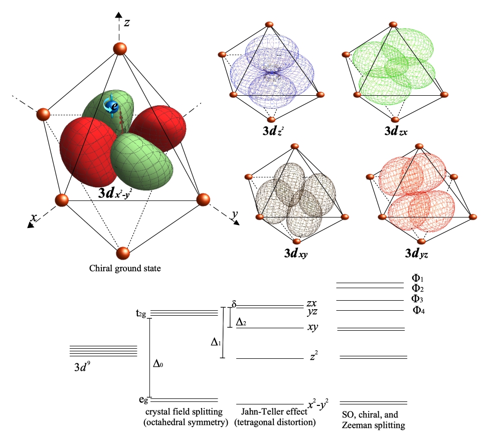
Figure 1: Energy levels of Cu(II) in a chiral quasi-octahedral configuration. Approximate experimental values are $\Delta_{0}\simeq 1.5$ eV, $\Delta_{1}\simeq 0.5$ eV, $\Delta_{2}\simeq≈0.23$ eV.

In our model, the $3d$ orbitals are represented by linear combinations of the $n=2$, $l=2$ states of the isotropic harmonic oscillator –see Appendix A. Essential to the original Condon model was the anisotropy of the harmonic oscillator, which removes all axis and planes of symmetry. In our model, such an anisotropy is provided by the interaction of the ion with the surrounding ligands of the complex, which in the case of CsCuCl₃ form an quasi-octahedral structure. In the first place, that interaction causes the elongation of the $3d$ orbitals which lie along the $z$-axis, opening an optical gap $\Delta_{0}$. Also, in conjunction with the Jahn-Teller distortion and the helical configuration of the Cu(II) ions, it removes the degeneracy between the orbitals lying on the $xy$ plane and generates a small energy gap $\delta$ between the states $d_{zx}$ and $d_{yz}$, with $\lambda\gg\delta$. The ground state of the Cu(II) ion in the octahedral configuration $\Psi$ is, at finite temperature and subject to a magnetic field, a linear combination of the doublet $d_{x^{2}-y^{2}}\otimes\{\uparrow,\downarrow\}$,

$$|\Psi\rangle=|d_{x^{2}-y^{2}}\rangle\otimes(\cos{\theta/2}\uparrow+\sin{\theta/2}\downarrow),$$ (6)

where $\theta$, being a function of $B_{0}$ and the temperature, is the angle between the magnetization of the sample and $\mathbf{B}_{0}$. For EPR, spin-flip takes place at a resonance frequency $\Omega=g\mu_{B}B_{0}/\hbar$ when the up $\uparrow$ component of $\Psi$ turns into $|\Phi\rangle=|d_{x^{2}-y^{2}}\rangle\otimes\downarrow$ , with probability proportional to $\cos^{2}\theta/2$, and the down $\downarrow$ component turns into $|\Phi^{\prime}\rangle=|d_{x^{2}-y^{2}}\rangle\otimes\uparrow$ with probability proportional to $\sin^{2}\theta/2$. The net absorption probability is thus proportional to $\cos^{2}\theta/2-\sin^{2}\theta/2=\cos\theta$ and hence to the degree of magnetization along $\mathbf{B}_{0}$. At  $B_{0}$ = 1T, $\Omega$ corresponds to an energy 150 $\mu$eV. In contrast, optical absorption happens at an energy $\Delta_{0}\simeq 1.5$ eV towards the quadruplet $\{d_{zx},d_{yz}\}\otimes\{\uparrow,\downarrow\}$. Applying standard perturbation theory with the spin-orbit and the Zeeman potentials upon this quasidegenerate quadruplet , we end up with the four states $\phi_{i}$, $i=1,..,4$, as appear in the energy diagram represented in Fig.1 –a brief description can be found in the Appendix A. It is of note that these states play a crucial role in the E1M1 transitions of both EPR and its optical analogue.

Results
Using up to fourth order time-dependent perturbation theory on $V_{SO}$, $V_{C}$ and $W$, in the adiabatic regime, our model allows us to calculate the standard EPR and optical transition probabilities, as well as the MChA corrections to both of them, with the latter two being both proportional to $C^{D/L}$. As for $g_{T}^{D/L}$, the probability difference in the denominator of Eq.(2) is an enantioselective E1M1 transition, whereas the denominator equals in good approximation the leading order M1M1 transition, $g_{T}^{D/L}=P_{E1M1}^{D/L}/P_{M1M1}|_{\omega\approx\Omega}$, with

$$P_{M1M1}|_{\omega\approx\Omega} =\hbar^{-2}\Bigl{|}\int_{0}^{\mathcal{T}}\text{d}te^{-i(\mathcal{T}-t)(\Omega/2-i\Gamma/2)}e^{-it(\omega-\Omega/2)}\langle\Phi|-g\mu_{B}\mathbf{S}\cdot\mathbf{B}_{\omega}|\Psi\rangle\Bigr{|}^{2}-\hbar^{-2}\Bigl{|}\int_{0}^{\mathcal{T}}\text{d}te^{-i(\mathcal{T}-t)(2\omega-\Omega/2-i\Gamma/2)}$$

$$\times e^{-it(\omega+\Omega/2)}\langle\Phi^{\prime}|-g\mu_{B}\mathbf{S}\cdot\mathbf{B}_{\omega}|\Psi\rangle\Bigr{|}^{2},$$

$$P_{E1M1}^{D/L}|_{\omega\approx\Omega} =-2\hbar^{-2}\text{Re}\int_{0}^{\mathcal{T}}\text{d}te^{-i(\mathcal{T}-t)(\Omega/2-i\Gamma/2)}\langle\tilde{\Phi}|-e\mathbf{r}\cdot(\bar{n}^{2}+2)\mathbf{E}_{\omega}/3|\tilde{\Psi}\rangle e^{-it(\omega-\Omega/2)}\int_{0}^{\mathcal{T}}\text{d}\tau\>e^{i(\mathcal{T}-\tau)(\Omega/2+i\Gamma/2)}$$

$$\times\langle\Psi|-g\mu_{B}\mathbf{S}\cdot\mathbf{B}_{\omega}^{\ast}|\Phi\rangle e^{i\tau(\omega-\Omega/2)}+2\hbar^{-2}\text{Re}\int_{0}^{\mathcal{T}}\text{d}t\>e^{-i(\mathcal{T}-t)(2\omega-\Omega/2)}\langle\tilde{\Phi}^{\prime}|-e\mathbf{r}\cdot(\bar{n}^{2}+2)\mathbf{E}_{\omega}/3|\tilde{\Psi}\rangle$$

$$\times e^{-it(\omega+\Omega/2-i\Gamma/2)}\int_{0}^{\mathcal{T}}\text{d}\tau\>e^{i(\mathcal{T}-\tau)(2\omega-\Omega/2)}\langle\Psi|-g\mu_{B}\mathbf{S}\cdot\mathbf{B}_{\omega}^{\ast}|\Phi^{\prime}\rangle e^{i\tau(\omega+\Omega/2+i\Gamma/2)},\quad\Gamma\mathcal{T}\gg 1,$$ (7)

where $\Gamma$ is the linewidth of EPR absorption, $\Gamma\mathcal{T}\gg 1$ implies the adiabatic approximation, and the states $\tilde{\Psi}$, $\tilde{\Phi}$, and $\tilde{\Phi}^{\prime}$ are dressed with the states $\phi_{i}$, $i=1,..,4$, on account of the spin-orbit and chiral interactions. Using a linearly polarized microwave probe field in Eq.(7), the resultant expression for the TWEEPR anisotropy factor reads

$$g_{T}^{D/L}\simeq\frac{c\,C^{D/L}\hbar\,\Omega\,\delta}{m_{e}\omega_{0}^{3}\Delta_{0}^{2}}\frac{\bar{n}^{2}+2}{3\bar{n}},$$ (8)

where the second factor on the right hand side describes the effect of the refractive index on the local electric field and the wavevector. It is worth noting that the aforementioned dependence on magnetization, $\sim\cos{\theta}$, cancels out in the ratio between probabilities. For further details, see Appendix B.

The values for the unknown parameters in Eq.(8) can be deduced comparing the predictions of the model with the experimental results for optical MChD MChD CsCuCl3 and EPR EPR CsCuCl3  in CsCuCl₃. In particular, we can estimate $g_{T}^{D/L}$ from the data on the non-reciprocal absorption coefficient in optical MChD, $\alpha_{A}=\alpha(\mathbf{B}_{0}\upharpoonleft\upharpoonright\mathbf{k})-\alpha(\mathbf{B}_{0}\downharpoonleft\upharpoonright\mathbf{k})$. The calculation goes as follows. In terms of the E1M1 absorption probability at resonance, $\omega=\Delta_{0}/\hbar$, $\alpha_{A}$ reads

$$\alpha_{A}=\frac{4c\mu_{0}\rho\Delta_{0}\Gamma^{\prime}}{|E_{\omega}|^{2}}P_{E1M1}^{D/L}|_{\omega=\Delta_{0}/\hbar},$$ (9)

where $\Gamma^{\prime}$ is the linewidth of optical absorption, and $\rho$ is the molecular number density of the complex. Using our model, a calculation analogous to that for $P_{E1M1}^{D/L,EPR}$ but for its optical counterpart, $P_{E1M1}^{D/L,O}$ – Appendices B, C and D-, allows as to express $g_{T}^{D/L}$ in Eq.(8) in terms of $\alpha_{A}$,

$$g_{T}^{D/L}=\frac{c\,\hbar^{3}\Gamma^{\prime}\Omega\tilde{\Delta}\alpha_{A}}{2\Delta_{0}^{3}\mu_{0}\mu_{B}^{2}\rho\cos{\theta}},$$ (10)

where $\tilde{\Delta}^{-1}=\Delta_{0}^{-1}+\Delta_{2}^{-1}-3\Delta_{1}^{-1}$ is the inverse of an effective energy interval which takes account of the optical transitions to intermediate states –see Fig.1. It is of note that, whereas the magnetic transition is driven in EPR by the spin operator [Eq.(7)], it is driven by the orbital angular momentum in the optical case. In turn, this causes MChD to be stronger in the optical case and proportional to the degree of magnetization $\cos{\theta}$, which can be approximated by $\cos{\theta}\approx\mu_{0}B_{0}/k_{B}T$ magnetization . The optical MChA parameter, $g_{0}^{D/L}$, has an analogous expression to that in Eq.(2) with $\hbar\omega\approx\Delta_{0}$, being proportional to $\alpha_{A}$. Hence, our model allows us to estimate its upper bound, $g_{0}^{D/L}\leq(cC^{D/L}\delta\cos{\theta})/(m_{e}\omega_{0}^{3}\tilde{\Delta})$ – see Appendices C and D, from which $g_{T}^{D/L}/g_{0}^{D/L}\gtrsim(\hbar\Omega\tilde{\Delta})/(\Delta_{0}^{2}\cos{\theta})$. Note that, since both $\Omega$ and $\cos{\theta}$ are proportional to $B_{0}$, the ratio between EPR and optical MChA factors is independent of the field strength.

Finally, substituting the experimental values for CsCuCl₃ of all the variables in Eq.(10), for $B_{0}=14$ T at a temperature of 4.2 K, we obtain $g_{T}^{D/L}\approx 1.5\cdot 10^{-2}$, which is small but not beyond the resolution of high field EPR spectrometers. For an X band EPR spectrometer ($B=0,35$ T), this means $g_{T}^{D/L}\approx 3\cdot 10^{-4\text{ }}$which will require a different approach, as we discuss below.

Implementation
In commercial EPR spectrometers, resonant standing wave cavities are used to enhance sensitivity. Such a cavity can be regarded as containing equal amounts of traveling waves with $\mathbf{k}$ and $-\mathbf{k.}$ The MChA $\gamma^{D/L}$ term in Eq.(1) can therefore not give a net contribution to the resonance in such a configuration. For this term to be observed, a traveling wave configuration should be used. Such configurations are not unknown in EPR; several reported home-built EPR spectrometers have used one-pass transmission configurations Early Transmission EPR Broadband EPR . Sensitivity for such a travelling wave configuration can be enhanced by means of a Mach-Zehnder interferometer Mach Zehnder or a unidirectional ring resonator Travelling resonator .

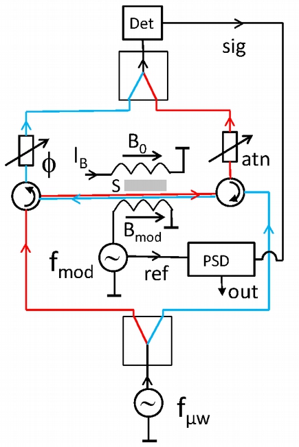
Figure 2: Schematic setup of the TWEEPR interferometer. The waves counterpropagating through the sample S are depicted in red and blue.

In such a configuration, MChA can be obtained as the difference between the microwave transmissions for the two opposing magnetic field directions, similar to what was realized in the optical case mcaabs . As the EPR lines can be quite narrow, the two oppositely oriented magnetic fields should have the same magnitude with high precision, which requires a tight control of this field, possibly with another EPR or NMR feedback circuit. Stabilizing a field this way can be quite time-consuming, and TWEEPR being a small difference on the already small EPR absorption, the extensive signal-averaging through field alternations that would be required to obtain a good signal-to-noise-ratio, makes such an approach impractical. We therefore propose another approach in the form of an X band microwave interferometer that removes the normal EPR contribution from the output signal, through destructive interference between counter-propagating waves through the sample at a fixed magnetic field, as illustrated in Figure 2. This leaves ideally only the TWEEPR contribution. By applying an additional small modulation field and using phase sensitive detection (PSD) sufficient sensitivity is obtained to resolve this small contribution. When tuned to total destructive interference at zero field, the interferometer output as given by the PSD is proportional to the TWEEPR response $d[T(\mathbf{B}_{0}\upharpoonleft\upharpoonright\mathbf{k})-T(\mathbf{B}_{0}\downharpoonleft\upharpoonright\mathbf{k})]/dB_{0}=\gamma^{D/L}(\omega)$. The sensitivity of the interferometer can be further improved by inserting the sample in a unidirectional resonant ring resonator. Q factors above $10^{3}$ have been reported for such configurations High Q ring and would bring a corresponding increase in sensitivity. It seems therefore quite feasible that TWEEPR can evolve into a standard characterization technique in the form of standalone dedicated TWEEPR spectrometers. An alternative to this configuration could be the microwave equivalent of the first observation of optical MChA in luminescence Naturemca , using pulsed EPR echo techniques EPR review with a similar interferometer setup.

Discussion
In general, the non-local response of a chiral system of size $a$ to an electromagnetic wave with wave vector $k$ is of the order $ka$, so one could have expected $g_{T}^{D/L}/g_{O}^{D/L}$ to be of the order $\hbar\Omega/\Delta_{0}$, the relevant spatial length scale for both TWEEPR and optical MChD being the orbital size. This ratio is of the order of $10^{-4}$, which would have put TWEEPR beyond experimental reach. However, in contrast to the optical absorption, which to zeroth order is independent of the magnetic field, the normal EPR absorption scales with the magnetization of the spin system. Since the MChA corrections are proportional to the magnetization in both EPR and the optical case, the cancellation of the factor $\cos{\theta\ll 1}$ applies to $g_{T}^{D/L}$ only, and it appears thereby in the denominator of $g_{T}^{D/L}/g_{O}^{D/L}$, resulting in Eq.(10). For room temperature X-band EPR of Cu(II), this results in $g_{T}^{D/L}/g_{O}^{D/L}$ of the order of $10^{-1}$, which makes TWEEPR experimentally feasible under those conditions. As a consequence, and in contrast to many other magnetic resonance techniques, going to low temperatures is not necessarily favorable for TWEEPR. Going to higher magnetic field does not affect $g_{T}^{D/L}/g_{O}^{D/L}$, the increase in $\Omega$ being compensated by the concomitant increase of $\cos{\theta}$ because of the higher resonance field.

The main results of our model are an analytic expression for the TWEEPR anisotropy factor [Eq.(8)] and an expression for its relationship with the optical anisotropy absorption coefficient [Eq.(10)]. The expression in Eq.(8) shows that $g_{T}^{D/L}$ has a linear dependence on the magnetic field strength (through $\Omega$) and on the chirality (through $C^{D/L}$), as predicted by symmetry arguments. The dependence on the spin-orbit coupling does not appear explicitly, because we have considered the case for Cu(II), where the level splitting $\delta$ is much smaller than the SO coupling $\lambda$. In the inverse case, $g_{T}^{D/L}$ would be proportional to $\lambda$ instead. Adapting the calculation to other chiral transition metal complexes is conceptually straightforward and should result in an expression similar to Eq.(8), apart from numerical factors of order unity. A rather different case is represented by chiral organic radicals, where the unpaired electron is delocalized on one or more interatomic bonds and a different microscopic model should be used for the calculation of $g_{T}^{D/L}$. One might however expect that such differences apply also to the calculation of $g_{O}^{D/L}$ for such radicals, preserving a relationship similar to that in Eq.(10).

Acknowledgements
This work was supported by the Agence Nationale de la Recherche (SECRETS, (ANR PRC 20-CE06-0023-01) and the Laboratory of Excellence NanoX (ANR-17-EURE-0009)). We gratefully acknowledge helpful discussions with Anne-Laure Barra.

In the Appendices we describe the theoretical model used in our calculations, we offer explicit expressions for the transition probabilities that enter the anisotropy factors in EPR and optical MChD, and comment on the limitations of our model.

Appendix A Fundamentals of the model

As outlined in the article, in order to estimate the MChA factors of a chiral Cu(II) complex, we consider a variant of the one-electron model proposed by Condon for the study of natural optical activity in chiral compounds Condon ; Condon2 . The total Hamiltonian of our model is $H=H_{0}+V_{C}^{D/L}+V_{SO}$, where $H_{0}=\frac{p^{2}}{2m_{e}}+\frac{m_{e}\omega_{0}^{2}r^{2}}{2}+V_{Z}$ is the unperturbed Hamiltonian, with $V_{Z}=-\mu_{B}(\mathbf{L}+g\mathbf{S)}\cdot\mathbf{B}_{0}$ being the Zeeman potential; and $V_{C}^{D/L}=C^{D/L}xyz,\>V_{SO}=\lambda\mathbf{L}\cdot\mathbf{S}$ being the chiral potential and the spin-orbit coupling, respectively. We stick to the nomenclature used in the article. The chiral Hamiltonian, $V_{C}^{D/L}$, results from the electrostatic interaction of the ion with the chiral configuration of the ligands in the complex, and produces the necessary parity asymmetry which is at the origin of natural optical activity. The orbital contribution of the Zeeman potential was added in Ref.Donaire EJP to the original Condon’s model to estimate the magneto-chiral birefringence of diamagnetic chiral compounds. In order to account for magnetochiral dichroism (MChD) in a paramagnetic complex, we introduce here the spin contribution to the Zeeman potential as well as the spin-orbit coupling. In contrast to the approach in Ref.Donaire EJP and for simplicity, we consider an isotropic harmonic oscillator, whereas the anisotropy caused by the crystal field is introduced in an effective manner through the energy intervals between the $3d$ orbitals, as depicted in Fig.1 in the article.

The eigenstates of $H_{0}$ are labeled with the eigenvalues of the orbital angular momentum and spin operators, $\{|n_{L},n_{R},n_{z}\rangle\}\otimes\{\uparrow,\downarrow\}$ Cohenbookvol2 , upon which $V_{C}^{D/L}$ and $V_{SO}$ act perturbatively. In a Cu(II) complex, the chromophoric charge is the unpaired electron of the $3d^{9}$ electronic configuration which behaves as a hole of positive charge. In the absence of ligands, the $3d$ orbitals of the ion can be represented approximately by the $n=2$, $l=2$ states of the harmonic oscillator of our model. However, the ligands’ fields affect the electronic configuration of the ion, removing the degeneracy of the $d$-states. In particular, for octahedral coordination geometries around the ion, the set of $d$-orbitals splits into doubly degenerate e_g orbitals, $d_{x^{2}-y^{2}}$ and $d_{z^{2}}$, and triply degenerate t_2g orbitals, $d_{xy}$, $d_{yz}$ and $d_{zx}$. The energy interval between e_g and t_2g states, $\Delta_{0}$, lies in the visible region of the spectrum, $\Delta_{0}\simeq 1.5$ eV. As a result, the e_g orbitals become the ground states, and can be approximated by linear combinations of $l=2$, $m_{l}=0,\pm 2$ eigenstates of the harmonic oscillator. The fact that the chromophoric charge in the e_g states cannot rotate into any other orbital leads to an effective quenching of the orbital angular momentum of the ground state. Below a certain temperature, an additional Jahn-Teller (JT) distortion takes place when the ligands along one of the axes, say the $z$-axis, move away from the ion in order to minimize the electronic repulsion, giving rise to the complete removal of the degeneracy in the e_g level, and to a partial lifting of the degeneracy in the t_2g orbitals. The isotropy of the system is thus broken and the ground state becomes unique, up to spin degeneracy. For the particular case of the CsCuCl₃ crystal, the bonds along the $z$-axis get elongated and the ground state is the $d_{x^{2}-y^{2}}$ orbital. Fig.1 in the article depicts the energy splitting of the distorted $d$-orbitals, including the approximate values of the energy intervals. Lastly, the JT distortion in conjuntion with the helical deformation of the crystal along the $c$-axis, of coordiates [1,1,1] in the local axis basis, removes the degeneracy between the orbitals lying on the $xy$ plane in a small ammount $\delta$. Below, we write the approximate expression of the $3d$ orbitals in terms of the harmonic oscillator eigenstates, $\{|n_{L},n_{R},n_{z}\rangle\}$, together with their corresponding energies,

$$|d_{zx}\rangle=(|0,1,1\rangle-|1,0,1\rangle)/\sqrt{2},\quad\mathcal{E}=\Delta_{0},$$

$$|d_{yz}\rangle=i(|0,1,1\rangle+|1,0,1\rangle)/\sqrt{2},\quad\mathcal{E}=\Delta_{0}-\delta,$$

$$|d_{xy}\rangle=i(|0,2,0\rangle-|2,0,0\rangle)/\sqrt{2},\quad\mathcal{E}=\Delta_{0}-\Delta_{2},$$

$$|d_{z^{2}}\rangle=(|1,1,0\rangle-\sqrt{2}|0,0,2\rangle)/\sqrt{3},\quad\mathcal{E}=\Delta_{0}-\Delta_{1},$$

$$|d_{x^{2}-y^{2}}\rangle=(|0,2,0\rangle+|2,0,0\rangle)/\sqrt{2},\quad\mathcal{E}=0.$$ (11)

Altogether, the crystal field combined with the JT distortion and the helical deformation turns the crystalline structure into a chiral one. In accord with Condon’s model, the potential $V^{D/L}_{C}$ reproduces the electrostatic interaction of the chromophoric charge with the surrounding chiral structure, removing all axes and planes of symmetry from the system. It is through the chiral potential that E1 transitions between the $3d$ orbitals take place in our model. In addition to the above interactions, MChD in EPR requires necessarily the coupling between the spin and the orbital angular momentum of the unpaired electron hole through the potential $V_{SO}$, where the coupling constant is $\lambda\approx-0.1$ eV. In particular, the SO interaction together with the Zeeman potential break the quasi-degeneracy between the four states $\{|d_{zx}\rangle,|d_{yz}\rangle\}\otimes\{\uparrow,\downarrow\}$, providing the following eigenstates for $\lambda\gg\delta$,

$$|\Phi_{1}\rangle \approx|1,0,1\rangle\otimes\downarrow+\frac{\delta}{2\lambda}|0,1,1\rangle\otimes\downarrow,\quad$$

$$\mathcal{E} \simeq\Delta_{0}-\lambda/2+\hbar\Omega,$$

$$|\Phi_{2}\rangle \approx|0,1,1\rangle\otimes\uparrow+\frac{\delta}{2\lambda}|1,0,1\rangle\otimes\uparrow,\quad$$

$$\mathcal{E} \simeq\Delta_{0}-\lambda/2-\hbar\Omega,$$

$$|\Phi_{3}\rangle \approx|0,1,1\rangle\otimes\downarrow-\frac{\delta}{2\lambda}|1,0,1\rangle\otimes\downarrow,\quad$$

$$\mathcal{E} \simeq\Delta_{0}+\lambda/2+\hbar\Omega+\frac{\delta^{2}}{4\lambda^{2}}(\lambda+\hbar\Omega),$$

$$|\Phi_{4}\rangle \approx|1,0,1\rangle\otimes\uparrow-\frac{\delta}{2\lambda}|0,1,1\rangle\otimes\uparrow,\quad$$

$$\mathcal{E} \simeq\Delta_{0}+\lambda/2-\hbar\Omega+\frac{\delta^{2}}{4\lambda^{2}}(\lambda-\hbar\Omega).$$ (12)

$\{\Phi_{1},\Phi_{2},\Phi_{3},\Phi_{4}\}$ are indeed the eigenstates of the Hamiltonian $V_{Z}+V_{SO}$ restricted to the subspace $\{|d_{zx}\rangle,|d_{yz}\rangle\}\otimes\{\uparrow,\downarrow\}$. They constitute the intermediate states of the transition processes in EPR mediated by the interaction of the spin with the chiral structure of the surrounding charges.

In the following, we apply to our system time-dependent quantum perturbation techniques to compute first the MChA factor in EPR, $g_{T}^{D/L}$. Next, in order to estimate the value of the unknowns of our model, we compute the anisotropy factor in optical MChD for the same system. Finally, making use of the experimental values available for CsCuCl₃ in the literature EPR CsCuCl3 ; MChD CsCuCl3 , we estimate the strength of TWEEPR.

Appendix B MChD in EPR

Let us consider a CsCuCl₃ complex, initially prepared in its ground state, and partially polarized along a uniform magnetic field $\mathbf{B}=B_{0}\hat{\mathbf{z}}$ directed along the $z$-axis,

$$|\Psi\rangle=|d_{x^{2}-y^{2}}\rangle\otimes(\cos{\theta/2}\uparrow+\sin{\theta/2}\downarrow)\approx\frac{1}{\sqrt{2}}(|0,2,0\rangle+|2,0,0\rangle)\otimes(\cos{\theta/2}\uparrow+\sin{\theta/2}\downarrow),$$ (13)

where we have approximated the actual ground state with the corresponding state of our harmonic oscillator model in the basis $\{|n_{L},n_{R},n_{z}\rangle\}\otimes\{\uparrow,\downarrow\}$, and $\theta$ is the angle between the magnetic moment of the complex and the $z$-axis, $\cos{\theta}=\hbar^{-1}\langle\Psi|2\mathbf{S}|\Psi\rangle\cdot\hat{\mathbf{z}}$. At temperature $T$, $\cos{\theta}\approx\mu_{0}B_{0}/k_{B}T$ magnetization . Under the action of an incident electromagnetic field of frequency $\omega$ close to the transition frequency, $\Omega=g\mu_{B}B_{0}/\hbar$, and wave vector $\mathbf{k}$ parallel to $\mathbf{B}_{0}$, the complex gets partially excited towards the state

$$|\Phi\rangle=|d_{x^{2}-y^{2}}\rangle\otimes\downarrow\approx\frac{1}{\sqrt{2}}(|0,2,0\rangle+|2,0,0\rangle)\otimes\downarrow,$$ (14)

with probability proportional to $\cos^{2}{\theta/2}$; and partially de-excited (through stimulated emission) towards the state

$$|\Phi^{\prime}\rangle=|d_{x^{2}-y^{2}}\rangle\otimes\uparrow\approx\frac{1}{\sqrt{2}}(|0,2,0\rangle+|2,0,0\rangle)\otimes\uparrow,$$ (15)

with probability proportional to $\sin^{2}{\theta/2}$. Since the rest of probability factors are equivalent, the net absorption probability in EPR is proportional to $\cos^{2}{\theta/2}-\sin^{2}{\theta/2}=\cos{\theta}$, and thus proportional to the magnetization of the complex.

As mentioned in the article, from symmetry considerations and in leading order, the numerator and the denominator in the ratio $g_{T}^{D/L}=[P^{D/L}(\omega,\hat{\mathbf{k}},\mathbf{B}_{0})-P^{D/L}(\omega,\hat{\mathbf{k}},-\mathbf{B}_{0})]/[P^{D/L}(\omega,\hat{\mathbf{k}},\mathbf{B}_{0})+P^{D/L}(\omega,\hat{\mathbf{k}},-\mathbf{B}_{0})]$ for $\omega\approx\Omega$ are dominated, respectively, by the electric-magnetic dipole (E1M1) and the magnetic-magnetic dipole (M1M1) transition probabilities, the magnetic transition being driven by the spin operator only. That leads to the approximate expression,

$$g_{T}^{D/L}\simeq\frac{P_{E1M1}^{D/L}(\omega,\hat{\mathbf{k}},\mathbf{B}_{0})}{P_{M1M1}(\omega,\hat{\mathbf{k}},\mathbf{B}_{0})}\Bigr{|}_{\omega\approx\Omega}.$$ (16)

In what follows, we compute the transition probabilities $P_{M1M1}$ and $P_{E1M1}^{D/L}$ for $\omega\approx\Omega$ using time-dependent perturbation theory in the adiabatic regime. This regime is the suitable one for a probe field whose duration is much longer than the typical lifetime for excitation or de-excitation. As in the article, the Hamiltonian of the interaction of our system with the microwave probe field reads, in the electric and magnetic dipole approximation, $W=-e\mathbf{r}\cdot\mathbf{E}_{\omega}(t)/2-\mu_{B}(\mathbf{L}+2\mathbf{S})\cdot\mathbf{B}_{\omega}(t)/2+$h.c.. In this equation, $\mathbf{E}_{\omega}(t)=\mathbf{E}_{\omega}e^{-i\omega t}=i\omega\mathbf{A}_{\omega}e^{-i\omega t}$, $\mathbf{B}_{\omega}(t)=\mathbf{B}_{\omega}e^{-i\omega t}=i\bar{n}\mathbf{k}\wedge\mathbf{A}_{\omega}e^{-i\omega t}$, are the complex-valued electric and magnetic fields, respectively, with $\mathbf{A}_{\omega}$ being the complex-valued amplitude of the plane-wave electromagnetic vector potential of frequency $\omega\approx\Omega$, evaluated at the center of mass of the Cu(II) ion, and $\bar{n}$ being the effective refractive index of the sample. The local depolarization changes the local electric field incident on each Cu(II) ion to $\mathbf{E}_{\omega}(\bar{n}^{2}+2)/3$. Under the action of $W$, with $\mathbf{k}$ along $\mathbf{B}_{0}$, the expressions for $P_{M1M1}$ and $P_{E1M1}^{D/L}$ read, respectively, at leading order in the coupling constants of the interaction potentials,

$$P_{M1M1}|_{\omega\approx\Omega} =\hbar^{-2}\left|\int_{0}^{\mathcal{T}}\text{d}te^{-i(\mathcal{T}-t)(\Omega/2-i\Gamma/2)}e^{-it(\omega-\Omega/2)}\langle\Phi|-g\mu_{B}\mathbf{S}\cdot\mathbf{B}_{\omega}|\Psi\rangle\right|^{2}$$

$$-\hbar^{-2}\left|\int_{0}^{\mathcal{T}}\text{d}te^{-i(\mathcal{T}-t)(2\omega-\Omega/2-i\Gamma/2)}e^{-it(\omega+\Omega/2)}\langle\Phi^{\prime}|-g\mu_{B}\mathbf{S}\cdot\mathbf{B}_{\omega}|\Psi\rangle\right|^{2},$$ (17)

$$P_{E1M1}^{D/L}|_{\omega\approx\Omega} =2\text{Re}(-i)^{3}\hbar^{-4}\sum_{p,q\neq\Psi}\int_{0}^{\mathcal{T}}\text{d}te^{-i(\mathcal{T}-t)(\Omega/2-i\Gamma/2)}\langle\Phi|-e\mathbf{r}\cdot(\bar{n}^{2}+2)\mathbf{E}_{\omega}/3|p\rangle\int_{-\infty}^{t}\text{d}t^{\prime}e^{\eta t^{\prime}}e^{-i(t-t^{\prime})(\mathcal{E}_{p}+\omega)}$$

$$\times\langle p|V^{D/L}_{C}|q\rangle\int_{-\infty}^{t^{\prime}}\text{d}t^{\prime\prime}e^{\eta t^{\prime\prime}}e^{-i(t^{\prime}-t^{\prime\prime})(\mathcal{E}_{q}+\omega)}\langle q|V_{SO}|\Psi\rangle e^{-it^{\prime\prime}(\omega-\Omega/2)}i\int_{0}^{\mathcal{T}}\text{d}\tau\>e^{i(\mathcal{T}-\tau)(\Omega/2+i\Gamma/2)}$$

$$\times\langle\Psi|-g\mu_{B}\mathbf{S}\cdot\mathbf{B}_{\omega}^{\ast}|\Phi\rangle e^{i\tau(\omega-\Omega/2)}\>+2\text{Re}(-i)^{3}\hbar^{-4}\sum_{p,q\neq\Phi}\int_{-\infty}^{\mathcal{T}}\text{d}t\>e^{\eta t}e^{-i(\mathcal{T}-t)(\Omega/2-i\Gamma/2)}\langle\Phi|V_{SO}|p\rangle$$

$$\times\int_{-\infty}^{t}\text{d}t^{\prime}e^{\eta t^{\prime}}e^{-i(t-t^{\prime})\mathcal{E}_{p}}\langle p|V^{D/L}_{C}|q\rangle\int_{0}^{t^{\prime}}\text{d}t^{\prime\prime}e^{-i(t^{\prime}-t^{\prime\prime})\mathcal{E}_{q}}\langle q|-e\mathbf{r}\cdot(\bar{n}^{2}+2)\mathbf{E}_{\omega}/3|\Psi\rangle e^{-it^{\prime\prime}(\omega-\Omega/2)}$$

$$\times i\int_{0}^{\mathcal{T}}\text{d}\tau\>e^{i(\mathcal{T}-\tau)(\Omega/2+i\Gamma/2)}\langle\Psi|-g\mu_{B}\mathbf{S}\cdot\mathbf{B}_{\omega}^{\ast}|\Phi\rangle e^{i\tau(\omega-\Omega/2)}$$

$$-2\text{Re}(-i)^{3}\hbar^{-4}\sum_{p,q\neq\Psi}\int_{0}^{\mathcal{T}}\text{d}t\>e^{-i(\mathcal{T}-t)(2\omega-\Omega/2)}\langle\Phi^{\prime}|-e\mathbf{r}\cdot(\bar{n}^{2}+2)\mathbf{E}_{\omega}/3|p\rangle\int_{-\infty}^{t}\text{d}t^{\prime}e^{\eta t^{\prime}}e^{-i(t-t^{\prime})(\mathcal{E}_{p}+\omega)}$$

$$\times\langle p|V^{D/L}_{C}|q\rangle\int_{-\infty}^{t^{\prime}}\text{d}t^{\prime\prime}e^{\eta t^{\prime\prime}}e^{-i(t^{\prime}-t^{\prime\prime})(\mathcal{E}_{q}+\omega)}\langle q|V_{SO}|\Psi\rangle e^{-it^{\prime\prime}(\omega+\Omega/2-i\Gamma/2)}i\int_{0}^{\mathcal{T}}\text{d}\tau\>e^{i(\mathcal{T}-\tau)(2\omega-\Omega/2)}$$

$$\times\langle\Psi|-g\mu_{B}\mathbf{S}\cdot\mathbf{B}_{\omega}^{\ast}|\Phi^{\prime}\rangle e^{i\tau(\omega+\Omega/2+i\Gamma/2)}\>-2\text{Re}(-i)^{3}\hbar^{-4}\sum_{p,q\neq\Phi^{\prime}}\int_{-\infty}^{\mathcal{T}}\text{d}t\>e^{\eta t}e^{-i(\mathcal{T}-t)(2\omega-\Omega/2)}$$

$$\times\langle\Phi^{\prime}|V_{SO}|p\rangle\int_{-\infty}^{t}\text{d}t^{\prime}e^{\eta t^{\prime}}e^{-i(t-t^{\prime})(2\omega+\mathcal{E}_{p})}\langle p|V^{D/L}_{C}|q\rangle\int_{0}^{t^{\prime}}\text{d}t^{\prime\prime}e^{-i(t^{\prime}-t^{\prime\prime})(2\omega+\mathcal{E}_{q})}$$

$$\times\langle q|-e\mathbf{r}\cdot(\bar{n}^{2}+2)\mathbf{E}_{\omega}/3|\Psi\rangle e^{-it^{\prime\prime}(\omega+\Omega/2-i\Gamma/2)}i\int_{0}^{\mathcal{T}}\text{d}\tau\>e^{i(\mathcal{T}-\tau)(2\omega-\Omega/2)}\langle\Psi|-g\mu_{B}\mathbf{S}\cdot\mathbf{B}_{\omega}^{\ast}|\Phi^{\prime}\rangle$$

$$\times e^{i\tau(\omega+\Omega/2+i\Gamma/2)},\quad\eta\rightarrow 0^{+},\>\>\Gamma\mathcal{T}\gg 1.$$ (18)

In these equations the states $p$ and $q$ stand for the excited states of the $3d^{9}$ configuration together with other eigenstates of $H_{0}$ with $n\neq 2$. The quasi-stationary condition $\eta\rightarrow 0^{+}$ accounts for the stationarity of the chiral and the spin-orbit interactions; whereas the adiabatic limit $\Gamma\mathcal{T}\gg 1$ takes into account the long duration of the probe field with respect to the lifetime $\Gamma^{-1}$, with $\Gamma$ being the linewidth of absorption and $\mathcal{T}$ the observation time. The diagrammatical representation of the processes involved in the above equation is given in Fig.3.

Figure 3: Diagrammatic representation of the processes which contribute to $P_{M1M1}$ and $P_{E1M1}^{D/L}$ for $\omega\approx\Omega$ at leading order in the perturbative interactions, i.e., at second order and fourth order, respectively. Time runs along the vertical direction from 0 to the observation time $\mathcal{T}$, where the probability is computed. Intermediate atomic states are labeled as $p$ and $q$. Diagrams with two-photon states account for stimulated emission.

In the article, the contributions of the quasi-stationary processes were incorporated into the dressed states $\tilde{\Psi}$, $\tilde{\Phi}$, $\tilde{\Phi}^{\prime}$. More specifically, the bare states are dressed with the quadruplet $\{\Phi_{1},..,\Phi_{4}\}$ through $V_{SO}$, and with harmonic states with $n\neq 2$ by $V_{C}$. In terms of the eigenstates of the harmonic oscillator, they read

$$|\tilde{\Phi}\rangle =\Bigr{[}(|020\rangle+|200\rangle)/\sqrt{2}+\frac{\lambda}{\sqrt{2}\Delta_{0}}(1+\Delta_{2}/\Delta_{0})(|020\rangle-|200\rangle)+\frac{i\lambda C^{D/L}K^{3/2}}{2\hbar\omega_{0}\Delta_{0}}(1+\Delta_{2}/\Delta_{0})$$

$$\times(|001\rangle-2|111\rangle)\Bigr{]}\downarrow\>+\>\Bigr{[}\frac{\lambda}{\sqrt{2}\Delta_{0}}(1+3\hbar\Omega/\Delta_{0})|011\rangle+\frac{\delta}{\sqrt{2}\Delta^{2}_{0}}(\hbar\Omega+\lambda/2)|101\rangle$$

$$+\frac{-iC^{D/L}K^{3/2}\lambda}{2\hbar\omega_{0}\Delta_{0}}(1+3\hbar\Omega/\Delta_{0})(|210\rangle-\sqrt{3}|030\rangle-\sqrt{2}|100\rangle)+\frac{iC^{D/L}K^{3/2}\delta}{2\hbar\omega_{0}\Delta^{2}_{0}}$$

$$\times(\hbar\Omega+\lambda/2)(|120\rangle-\sqrt{3}|300\rangle-\sqrt{2}|010\rangle)\Bigr{]}\uparrow$$

$$|\tilde{\Phi}^{\prime}\rangle =\Bigr{[}(|020\rangle+|200\rangle)/\sqrt{2}+\frac{-\lambda}{\sqrt{2}\Delta_{0}}(1+\Delta_{2}/\Delta_{0})(|020\rangle-|200\rangle)+\frac{-i\lambda C^{D/L}K^{3/2}}{2\hbar\omega_{0}\Delta_{0}}(1+\Delta_{2}/\Delta_{0})$$

$$\times(|001\rangle-2|111\rangle)\Bigr{]}\uparrow\>+\>\Bigr{[}\frac{-\lambda}{\sqrt{2}\Delta_{0}}(1-3\hbar\Omega/\Delta_{0})|101\rangle+\frac{\delta}{\sqrt{2}\Delta^{2}_{0}}(\hbar\Omega-\lambda/2)|011\rangle$$

$$+\frac{-iC^{D/L}K^{3/2}\lambda}{2\hbar\omega_{0}\Delta_{0}}(1-3\hbar\Omega/\Delta_{0})(|120\rangle-\sqrt{3}|300\rangle-\sqrt{2}|010\rangle)+\frac{-iC^{D/L}K^{3/2}\delta}{2\hbar\omega_{0}\Delta^{2}_{0}}$$

$$\times(\hbar\Omega-\lambda/2)(|210\rangle-\sqrt{3}|030\rangle-\sqrt{2}|100\rangle)\Bigr{]}\downarrow$$

$$|\tilde{\Psi}\rangle =\cos{\theta/2}|\tilde{\Phi}^{\prime}\rangle+\sin{\theta/2}|\tilde{\Phi}\rangle,\qquad K=\hbar/(2m_{e}\omega_{0}).$$ (19)

Using a linearly polarized incident field and averaging in orientations around the $\hat{\mathbf{z}}$-axis, we obtain, for $\lambda\gg\delta$,

$$P_{M1M1}|_{\omega\approx\Omega} \simeq\frac{\hbar^{-2}\mu_{B}^{2}|B_{\omega}|^{2}}{4[(\omega-\Omega)^{2}+\Gamma^{2}/4]}\cos{\theta},$$ (20)

$$P_{E1M1}^{D/L}|_{\omega\approx\Omega} \simeq\frac{(\bar{n}^{2}+2)}{3}\frac{C^{D/L}\Omega\delta}{m_{e}\omega_{0}^{3}\Delta_{0}^{2}}\frac{\hbar^{-1}\mu_{B}^{2}|B_{\omega}||E_{\omega}|}{4[(\omega-\Omega)^{2}+\Gamma^{2}/4]}\cos{\theta},$$ (21)

$$g_{T}^{D/L} \simeq\frac{(\bar{n}^{2}+2)}{3\bar{n}}\frac{c\,C^{D/L}\hbar\Omega\delta}{m_{e}\omega_{0}^{3}\Delta_{0}^{2}}+\mathcal{O}(\delta/\lambda,\lambda/\Delta_{0}).$$ (22)

Lastly, it is worth mentioning that for the case $\delta>\lambda$, i.e., when anisotropy dominates over the spin-orbit coupling, $g_{T}^{D/L}$ scales as $(c\hbar C^{D/L}\Omega\delta\lambda)/(m_{e}\omega_{0}^{3}\Delta_{0}^{3})$ instead. This scenario will be addressed in a separate publication inpreparation .

Appendix C Optical MChD

Optical MChD involves transitions of frequency $\Delta_{0}$ from the ground state $|\Psi\rangle$ to the quasi-degenerate quadruplet $\{|d_{zx}\rangle,|d_{yz}\rangle\}\otimes\{\uparrow,\downarrow\}$ which, in account of the Zeeman and spin-orbit interactions, for $\delta\ll\lambda$, corresponds to the set of states $\{\Phi_{1},...,\Phi_{4}\}$ of Eq.(12). In contrast to EPR, the absorption probability in the denominator of the ratio $g_{O}^{D/L}=[P^{D/L}(\omega,\hat{\mathbf{k}},\mathbf{B}_{0})-P^{D/L}(\omega,\hat{\mathbf{k}},-\mathbf{B}_{0})]/[P^{D/L}(\omega,\hat{\mathbf{k}},\mathbf{B}_{0})+P^{D/L}(\omega,\hat{\mathbf{k}},-\mathbf{B}_{0})]$ for $\omega\approx\Delta_{0}/\hbar$ may not be dominated by the magnetic-magnetic dipole absorption probability. This might be so because the $d$-orbitals of the Cu(II) ion hybridize generally with the $\sigma$ and $\pi$ orbitals of the ligands, allowing for additional electric-electric dipole (E1E1) transitions. For the sake of simplicity, we will neglect the latter in our calculations, which implies that our preliminar estimate for $g_{O}^{D/L}$ must be intended as an approximate upper bound. As for the case of EPR, the numerator of the ratio in $g_{O}^{D/L}$ is again dominated by the electric-magnetic dipole absorption probability, and the non-vanishing terms come from magnetic transitions driven by the spin angular momentum –Eq.(24) below. However, in contrast to EPR, the magnetic transitions in the denominator are mainly driven by the orbital angular momentum operator –see Eq.(23) below. In turn, this causes the E1M1 transition probability to depend on the spin polarization of the complex, whereas neither the M1M1 nor the E1E1 probabilities do. Note also that stimulated emission from the state $|\Psi\rangle$ is absent in optical MChD. All in all, this implies that $g_{O}^{D/L}$ is proportional to the magnetization of the sample, which is itself proportional to the degree of spin-polarization along $\mathbf{B}_{0}$, $\cos{\theta}$, in agreement with experiments.

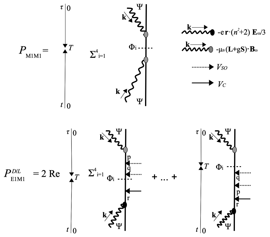
Figure 4: Diagrammatic representation of $P_{M1M1}$ and $P_{E1M1}^{D/L}$ for $\omega\approx\Delta_{0}/\hbar$ at leading order in the perturbative interactions, i.e., at second and up to fifth order, respectively. Intermediate atomic states are labeled as $p,q,r,s$.

In Fig.4 we depict some of the diagrams which contribute to $P_{M1M1}$ and $P_{E1M1}^{D/L}$ in optical MChD. Following a perturbative approach analogous to that in EPR, for an incident electromagnetic plane wave with $\mathbf{k}\parallel\mathbf{B}_{0}$ and assuming $\delta\ll\lambda$, one arrives at

$$P_{M1M1}|_{\omega\approx\Delta_{0}/\hbar} \simeq\frac{\hbar^{-2}\mu_{B}^{2}|B_{\omega}|^{2}}{4[(\omega-\Delta_{0}/\hbar)^{2}+\Gamma^{{}^{\prime}2}/4]},$$ (23)

$$P_{E1M1}^{D/L}|_{\omega\approx\Delta_{0}/\hbar} \simeq\frac{(\bar{n}^{2}+2)}{3}\frac{C^{D/L}\delta}{2m_{e}\omega_{0}^{3}\tilde{\Delta}}\frac{\hbar^{-2}\mu_{B}^{2}|B_{\omega}||E_{\omega}|}{4[(\omega-\Delta_{0}/\hbar)^{2}+\Gamma^{{}^{\prime}2}/4]}\cos{\theta},$$ (24)

$$g_{O}^{D/L} \lesssim\frac{P_{E1M1}^{D/L,O}}{P_{M1M1}^{O}}\Bigr{|}_{\omega\approx\Delta_{0}/\hbar}\simeq\frac{(\bar{n}^{2}+2)}{3\bar{n}}\frac{c\,C^{D/L}\delta\cos{\theta}}{2\,m_{e}\omega_{0}^{3}\tilde{\Delta}},$$ (25)

where $\tilde{\Delta}^{-1}=\Delta_{0}^{-1}+\Delta_{2}^{-1}-3\Delta_{1}^{-1}$, and $\Gamma^{\prime}$ is the linewidth of optical absorption. As anticipated, the fact that the magnetic dipole transition in $P_{E1M1}^{D/L}$ is dominated by the orbital angular momentum operator causes its leading order term to depend on the magnetization $\sim\cos{\theta}$. Hence, time-reversal invariance happens to be broken by the spin-polarization of the complex.

Appendix D Estimate of $g_{T}^{D/L}$

In the first place, we work out the relationship between $g^{D/L}_{T}$ and $g^{D/L}_{O}$. Comparing Eq.(21) with Eq.(24) at resonance, and taking into account Eqs.(22) and (25), we arrive at the following relationships,

$$\frac{P_{E1M1}^{D/L}|_{\omega=\Omega}}{P_{E1M1}^{D/L}|_{\omega=\Delta_{0}/\hbar}}\simeq\frac{2\hbar\Omega\tilde{\Delta}\Gamma^{{}^{\prime}2}}{\Delta_{0}^{2}\Gamma^{2}},\qquad\frac{g_{T}^{D/L}}{g_{O}^{D/L}}\gtrsim\frac{2\hbar\Omega\tilde{\Delta}}{\Delta_{0}^{2}\cos{\theta}}.$$ (26)

Next, considering the experimental data obtained in Ref.MChD CsCuCl3 for $g_{O}^{D/L}$ and applying the relationship in Eq.(26), we can estimate a lower bound for $g_{T}^{D/L}$. That is, substituting into Eq.(26) the experimental values $g_{O}^{D/L}\approx 0.025$, $\cos{\theta}\approx 0.4$, for $B_{0}=14$T at a temperature of 4.2 K, we obtain $g_{T}^{D/L}\gtrsim 10^{-4}$.

Alternatively, we can estimate $g_{T}^{D/L}$ using the experimental data of Ref.MChD CsCuCl3 for the non-reciprocal absorption coefficient of optical MChD, $\alpha_{A}=\alpha(\mathbf{B}_{0}\upharpoonleft\upharpoonright\mathbf{k})-\alpha(\mathbf{B}_{0}\downharpoonleft\upharpoonright\mathbf{k})$. In order to do so, we first write down $\alpha_{A}$ as a function of $P_{E1M1}^{D/L,O}$ at resonance,

$$\alpha_{A}=\frac{4c\mu_{0}\rho\Gamma^{\prime}\Delta_{0}}{|E_{\omega}|^{2}}P_{E1M1}^{D/L}|_{\omega=\Delta_{0}/\hbar},$$ (27)

where $\rho$ is the molecular density of the CsCuCl₃ complex (mass density 3.5g/cm³). Substituting the expression for $P_{E1M1}^{D/L,O}(\omega=\Delta_{0}/\hbar)$ in the above equation and using Eq.(22) we arrive at the equalities,

$$C^{D/L}\delta\ =\frac{3\hbar^{2}m_{e}\omega_{0}^{3}\tilde{\Delta}\Gamma^{\prime}\alpha_{A}}{2(\bar{n}^{2}+2)\rho\mu_{0}\mu_{B}^{2}\Delta_{0}\cos{\theta}},\quad g_{T}^{D/L}\ =\frac{c\,\hbar^{3}\Gamma^{\prime}\Omega\tilde{\Delta}\alpha_{A}}{2\Delta_{0}^{3}\mu_{0}\mu_{B}^{2}\rho\cos{\theta}}.$$ (28)

Substituting the experimental values for all the variables in Eq.(28), for $B_{0}=14\,$T at a temperature of $4.2\,$K, with $\Gamma^{\prime}\approx 0.1$eV and $\bar{n}\approx 1.5$, we obtain $g_{T}^{D/L}\approx 1.5\cdot 10^{-2}$, in agreement with our previous lower bound estimate.

Appendix E Further comments on the Hamiltonian model

Despite the success of our model to derive analytical estimates for the MChA factors, there is still room for improvement. In the first place, concerning the chiral Hamiltonian $V_{C}$, it was written in terms of the local axis of the octahedral structure, $x$, $y$, $z$, while it should be adapted to the crystal axis to account for the helical distribution of the active ions along the $c$-axis. In fact, the experimental data on $\alpha_{A}$ taken from the literature to estimate $g_{T}^{D/L}$ consider $\mathbf{B}_{0}$ along the $c$-axis. Also, the harmonic oscillator model, which is considered only distorted in the $n=2,l=2$ level, may not be accurate enough to account for the intermediate transitions induced by the chiral potential to levels with $n\neq 2$. Hence, a more accurate confining potential model, though less generic, can be obtained using a more detailed formulation of the crystal field and the JT distortion for the particular case of CsCuCl₃–see, eg., Ref.Maaskant . Finally, our estimate of the unknown combination $C^{D/L}\delta$ in terms of $\alpha_{A}$ [Eq.(28)], involves $\bar{n}$-dependent factors [Eq.(22], which account for effective incident fields, as well as $\rho$-dependent factors. For high densities and $\bar{n}\approx 1.5$ those factors are likely to depend on near field terms and spatial correlations when evaluated at the absorption frequency MePRA .

References

(1) Many excellent EPR books and reviews exist, one of the
most recent is EPR Spectroscopy: Fundamentals and Methods eds. D.
Goldfarb and S. Stoll, Wiley Chichester 2018.
(2)Spin labeling, Biological Magnetic
Resonance vol. 14 ed L. Berliner, Kluwer, New York 2002.
(3)Biomolecular EPR spectroscopy, W. R. Hagen,
CRC Boca Raton 2009.
(4) M.P. Groenewege, Mol. Phys. 5, 541 (1962).
(5) D.L. Portigal and E. Burstein, J. Phys. Chem. Solids
32, 603 (1971).
(6) N.B. Baranova, Yu. V. Bogdanov, B. Ya. Zeldovich, Opt.
Commun. 22, 243 (1977).
(7) G. Wagnière and A. Meier, Chem. Phys. Lett. 93, 78 (1982).
(8) L. D. Barron and J. Vrbancich, Mol. Phys. 51, 715
(1984).
(9) G.L.J.A. Rikken and E. Raupach, Nature 390, 493
(1997).
(10) P. Kleindienst and G. Wagnière, Chem. Phys. Let.
288, 89 (1998).
(11) G.L.J.A. Rikken and E. Raupach , Phys. Rev. E 58,
5081-5084 (1998).
(12) S. Tomita, K. Sawada, A. Porokhnyuk, and T. Ueda,
Phys. Rev. Lett. 113, 235501 (2014). Y. Okamura, F. Kagawa, S.
Seki, M. Kubota, M. Kawasaki, and Y. Tokura, Phys. Rev. Lett. 114,
197202 (2015).
(13) M. Ceolín, S. Goberna-Ferrón and J. R. Galán-Mascarós, Adv. Mat. 2012, DOI: 10.1002/adma.201200786, R. Sessoli, M.
Boulon, A. Caneschi, M. Mannini, L. Poggini, F.Wilhelm and A. Rogalev, Nat.
Phys. 11, 69 (2015).
(14) G.L.J.A. Rikken, J. Fölling and P. Wyder, Phys. Rev.
Lett. 87, 236602 (2001).
(15) V. Krstić, S. Roth, M. Burghard, K. Kern and
G.L.J.A. Rikken, J. Chem. Phys. 117, 11315 (2002).
(16) F. Pop, P. Auban-Senzier, E. Canadell, G. L. J. A. Rikken and
N. Avarvari, Nat. Comm. 5, 3757 (2014).
(17) T. Yokouchi, N. Kanazawa, A. Kikkawa, D. Morikawa, K.
Shibata, T. Arima, Y. Taguchi, F. Kagawa, Y. Tokura, Nat. Comm. 8,
866 (2017).
(18) H. Maurenbrecher, J. Mendil, G. Chatzipirpiridis, M.
Mattmann, S. Pané, B. J. Nelson, and P. Gambardella, Appl. Phys. Lett.
112, 242401 (2018).
(19) R. Aoki,1 Y. Kousaka and Y. Togawa, Phys. Rev. Lett. 122,
057206 (2019).
(20) G.L.J.A. Rikken and N. Avarvari, Phys. Rev. B
(2019).
(21) T. Nomura, X.-X. Zhang, S. Zherlitsyn, J. Wosnitza, Y.
Tokura, N. Nagaosa, and S. Seki, Phys. Rev. Lett. 122, 145901 (2019).
(22) G.L.J.A. Rikken and N. Avarvari, Nat. Comm. 13,
3564 (2022).
(23) W. Roy Mason, A practical guide to magnetic circular dichroism, Wiley 2008.
(24) N. Nakagawa et al, Phys. Rev. B 96,
121102(R) (2017).
(25) H. Tanaka, U. Schotte and K.D. Schotte, J. Phys. Soc.
Japan 61, 1344 (1992).
(26) E.U. Condon, Rev. Mod. Phys. 9, 432 (1937).
(27) E. U. Condon, William Altar, and Henry Eyring, J. Chem.
Phys. 5, 753 (1937).
(28) M. Donaire, G. L.J.A. Rikken, and B. A. van Tiggelen,
Eur. Phys. J. D 68, 33 (2014).
(29) C. Cohen-Tannoudji, B. Diu, F. Laloe, Quantum
Mechanics, Wiley-VCH (1992).
(30) M. Donaire and G. L.J.A. Rikken, in preparation.
(31) S. Toyoda, N. Abe, S. Kimura, Y.H. Matsuda, T.
Nomura, A. Ikeda, S. Takeyama, and T. Arima, Phys. Rev. Lett. 115,
267207 (2015); A. Sera, Y. Kousaka, J. Akimitsu, M. Sera, T. Kawamata, Y.
Koike, and K. Inoue, Phys. Rev. B94, 214408 (2016).
(32) Pake, G. E.; Townsend, J.; Weissman, S. I.
Phys. Rev.85, 682 (1952), Bogle, G. S., Symmons, H. F.,
Burgess, V. R.; Sierins, J. V., Proc. Phys. Soc. London 77,
561(1961), Chamberlain, J. R.; Syms, C.H.A., Proc. Phys. Soc., London84, 867 (1964), Rao, K. V. S., Sastry, K. V. L. N., Chem.
Phys. Lett. 6,485.(1970), Bramley, R.; Strach, S. J. Chem. Phys. Lett.79, 183 (1981).
(33) Y. Wiemann, J. Simmendinger, C. Clauss, L. Bogani,
D. Bothner, D. Koelle, R. Kleiner, M. Dressel and M. Scheffler, Appl. Phys.
Lett. 106, 193505 (2015)
(34) Zhe Chen, Jiwei Sun, and Pingshan Wang, IEEE Trans.
Mag. 53, 4001909 (2017), P. R. Shrestha, N. Abhyankar, M. A.
Anders,K. P. Cheung, R. Gougelet, J. T. Ryan, V. Szalai,and J. P. Campbell,
Anal. Chem. 91, 11108 (2019).
(35) E. N. Shaforost, N. Klein, S. A. Vitusevich,
A. Offenhäusser, and A. A. Barannik, J. Appl. Phys. 104, 074111
2008.
(36) Hee-Jo Lee, Kyung-A Hyun, and Hyo-Il Jung, Appl. Phys.
Lett. 104, 023509 (2014).
(37) W.J.A. Maaskant, and W.G. Haije, J. Phys. C: Solid State
Phys. 19, 5295 (1986).