A Quantum Algorithm for Shapley Value Estimation

Abstract

The introduction of the European Union’s (EU) set of comprehensive regulations relating to technology, the General Data Protection Regulation, grants EU citizens the right to explanations for automated decisions that have significant effects on their life. This poses a substantial challenge, as many of today’s state-of-the-art algorithms are generally unexplainable black boxes. Simultaneously, we have seen an emergence of the fields of quantum computation and quantum AI. Due to the fickle nature of quantum information, the problem of explainability is amplified, as measuring a quantum system destroys the information. As a result, there is a need for post-hoc explanations for quantum AI algorithms. In the classical context, the cooperative game theory concept of the Shapley value has been adapted for post-hoc explanations. However, this approach does not translate to use in quantum computing trivially and can be exponentially difficult to implement if not handled with care. We propose a novel algorithm which reduces the problem of accurately estimating the Shapley values of a quantum algorithm into a far simpler problem of estimating the true average of a binomial distribution in polynomial time.

1 Introduction

1.1 Background

With the introduction of the European Union’s set of comprehensive regulations relating to technology, the General Data Protection Regulation (GDPR), there has been a massive shift in the world of AI. Specifically in our case, the GDPR has provided EU citizens a right to explanation goodman2017european . This poses a substantial challenge, as many of today’s state of the art algorithms, such as Deep learning models, are generally black boxes rudin2019stop . Meaning that even the developers of AI models usually have no way of actually understanding the decisions of their models. There are two paths one can take to rectify the new need for model explanations, either by making models inherently interpretable, or by coming up with post-hoc explanations for our black-box models. One more recent axiomatic strategy for post-hoc explainability is based on the game theory concept of the Shapley value which is a powerful measure of contribution lundberg2017unified . However, direct calculation of Shapley values is an NP-hard problem matsui2001np ; prasad1990np , and outside of specific problems types, sampling is the only option for approximating Shapley values castro2009polynomial .

On the other hand, we have the emergence of quantum algorithms and quantum machine learning (QML) biamonte2017quantum . Quantum computers are at least naively resistant to explanation, as the even measuring the internal state destroys most of the information within it. Combining this with techniques like deep reinforcement learning with variational quantum circuits chen2020variational makes interpretability seem impossible.

1.2 Problem Statement

Inherently interpretable models would likely be best rudin2019stop , as an explanation of an interpretable model is guaranteed to be correct. However, much of the research and work in AI over the past couple decades have been into black box models, and many of the benefits of QML may not be possible to implemented in an interpretable fashion. Ideally, we do not want to throw away all of the previous black box research, so there is value in implementing and improving post-hoc explanation methods.

Current solutions to post-hoc explanations would unintuitive, or unwieldy to apply in the context of quantum computers. We explore a native quantum solution to post-hoc explainability using Shapley value approximation, where the function itself is approximated.

1.3 Results

We develop a flexible framework for global evaluation of input factors in quantum circuits which approximates the Shapley values of such factors. Our framework increases circuit complexity by an additional roughly $O(nlogn)$ c-not gates, with a total increase in circuit depth of $O(n)$, where $n$ is the number of factors. The change in space complexity for global evaluations is an additional $O(logn)$ qubits over the circuit being evaluated. This is in stark contrast to the $O(2^{n})$ assessments needed to directly assess the Shapley values under the general case.

1.4 Paper Organization

Section 2 provides the background and preliminaries. Sections 3 and 4 present our quantum algorithm, including an analytic analysis. Section 5 provide some examples. Section 6 concludes the work.

2 Background

2.1 Shapley Values

2.1.1 Cooperative Game Theory

Cooperative game theory is the study of coalitional games.

Definition 1.

A coalitional game can be described as the tuple $G=(F,V)$, wherein $F=\{1,2,...,N\}$ is a set of $N$ players. $V$ is a value function with $V(S)\in\mathbb{R}$ representing the value of a given coalition $S\subseteq F$, with the restriction that $V(\emptyset)=0$.

Definition 2.

Given a game $G=(F,V)$, $F=\{1,2,\dots,N\}$, a payoff vector $\Phi(G)$ is a vector of length $N$, which describes the utility $\Phi(G)_{i}$ of player $i$. A payoff vector is determined by the value function, where player $i$’s payoff value $\Phi(G)_{i}$ is determined by how $V(S)\>S\subseteq F$ is effected by $i$’s inclusion or exclusion from $S$ for any possible $S$.

There are various solution concepts that construct these payoff vectors (or sets of payoff vectors) aumann2010some . In this paper, we are most interested in Shapley values.

2.1.2 Shapley Values

In the early 50s, Shapley introduced a new solution concept to determine resource allocation in cooperative games which we now denote the Shapley value. It was unique in that it returned a single unique payoff vector, which was thought to be potentially untenable at the time winter2002shapley .

The Shapley value can be derived by the use of one of several sets of axioms, in our case we use the following four. Suppose we have games $G=(F,V)$ and $G^{\prime}=(F,V^{\prime})$, $F=\{1,2,\dots,N\}$, and a payoff vector $\Phi(G)$, then:

1. Efficiency: The sum of all utility is equal to the utility of the grand coalition

   $$\sum\limits_{i=1}^{N}\Phi(G)_{i}=V(F)$$

2. Equal Treatment: Players i, j are said to be symmetrical if $\forall_{S\subseteq F,\>i,j\notin S}[V(S\cup\{i\})=V(S\cup\{j\})]$. If i, and j are symmetric in G, then they are treated equally:

   $$\Phi(G)_{i}=\Phi(G)_{j}$$

3. Null Player: If player $i$ satisfies $\forall_{S\in F,\>i\notin S}[V(S)=V(S\cup\{i\})]$, then $i$ is a null player. If $i$ is a null player then:

   $$\Phi(G)_{i}=0$$

4. Additivity: If a player is in two games the Shapley values between the two games is additive:

   $$\Phi(G+G^{\prime})_{i}=\Phi(G)_{i}+\Phi(G^{\prime})_{i}$$

   Where a game $G+G^{\prime}$ is defined as $G=(F,V+V^{\prime})$, and $(V+V^{\prime})(S)=V(S)+V^{\prime}(S)$, $S\subseteq F$.

Amazingly, these axioms lead to a single unique and quite intuitive division of utility winter2002shapley . Even more, the Shapley value of $i$ turns out to be the expected marginal contribution to a random coalition $S\subseteq F\setminus\{i\}$, where marginal contribution $=V(S\cup\{i\})-V(S)$. This can be interpreted as a fair division of utility hart1989shapley .

2.1.3 Direct Calculation

It can be shown that the following equation gives us the payoff vector for the Shapley value solution concept, which we will call Shapley values shapley1952value ; lipovetsky2001analysis .

Definition 3.

Let $G=(F,V)$, for simplicity sake, we will now write $\Phi(G)_{i}$ as $\Phi_{i}$. Then, the Shapley value of the $i^{th}$ factor $\Phi_{i}$ can be described as:

$$\Phi_{i}=\sum\limits_{S\subseteq F\setminus\{i\}}\gamma(\lvert F\setminus\{i\}\rvert,\lvert S\rvert)\cdot(V(S\cup\{i\})-V(S))$$

Where,

$$\gamma(n,m)=\frac{1}{{n\choose m}(n+1)}=\frac{m!(n-m)!}{(n+1)!}$$

The Shapley value can be interpreted as a weighted average of contributions. The weights themselves have an intuitive interpretation, the $\frac{1}{{n\choose m}}$ results in each possible size of $S$ having an equal impact on the final value (since given $\lvert S\rvert=m$, there would be ${n\choose m}$ summands contributing to the final value). The $\frac{1}{n+1}$ averages between the different sizes of $S$.

2.1.4 Intractability

Unfortunately, in spite of all the desirable attributes of Shapley values it has a major weakness, it can be incredibly costly to compute. With the above formulation one would need to assess $V$ with $2^{\lvert F\setminus\{i\}\rvert}$ different subsets. In general, except for very specific circumstances, there seems to be no clever solutions or reformulations either. Deterministically Computing Shapley values in the context of weighted voting games has been shown to be NP-complete matsui2001np ; prasad1990np . Considering voting games are some of the most simple cooperative games, this result does not bode well for more complex scenarios. In the context of Shapley values for machine learning, it has also been shown that calculation of Shapley values are not tractable for even regression models van2022tractability . It was also proven that in an empirical setting finding Shapley values is exponential bertossi2020causality .

2.2 Explainable AI

The importance of eXplainable AI (XAI) is multifaceted, on the one hand, actually understanding a model’s reasoning allows for more robustness. This can be intuited simply with the following thought experiment: imagine implementing a traditional program without being able to understand what the computer is doing, where it is literally impossible to debug. If by some miracle you were able to get it working, it certainly would not be robust to edge cases. This is more or less the situation data scientists and engineers are in while developing large black box models, they are stuck with at best naive and heuristic strategies for debugging, without a good way of understanding what the model is doing or why. XAI, in particular post-hoc explanations can serve as a critical debugging tool kulesza2015principles ; goebel2018explainable . On the other hand in important, potentially life altering applications such as medicine, loan decisions, law, and various other critical fields we can not afford to rely on AI which we don’t understand. This is not only because of the recent legislative shift with the GDPR hoffman2018metrics , but for the obvious moral and practical reasons.

3 A Quantum Algorithm for Shapley Value Estimation

Consider a game with $G=(F,V)$, $F=\{0,1,\dots,n\}$, note that this is a game of $n+1$ players. The goal is to efficiently approximate the Shapley value of a given player $i$. Suppose a quantum version of $V$, $U^{\pm}_{V}$, is given, such that:

$$U^{\pm}_{V}\ket{x}\ket{0}:=\ket{x}\left(\sqrt{\frac{1-\hat{V}^{\pm}(x)}{2}}\ket{0}+\sqrt{\frac{1+\hat{V}^{\pm}(x)}{2}}\ket{1}\right)$$

where $\ket{x}$ is a vector in the computational basis. Define $V_{\text{max}}$ to be an upper bound for the value function magnitude.

$$V_{\text{max}}\geq\max\limits_{S\subseteq F}\lvert V(S)\rvert$$

Consider the binary integer, $x=x_{0}x_{1}\dots x_{i-1}x_{i+1}\dots x_{n}$, let $S_{x}$ be the set of all players $j$ such that $x_{j}=1$. This binary subset encoding can represent every player coalition which excludes player $i$. Next, define,

$$\hat{V}^{+}(x):=\frac{V\left(S_{x}\cup\{i\}\right)}{V_{\text{max}}},\text{ and }\hat{V}^{-}(x):=\frac{V\left(S_{x}\right)}{V_{\text{max}}}.$$

A critical step for the algorithm is to approximate the weights of the Shapley value function. As will be shown later, these Shapley weights correspond perfectly to a slightly modified beta function:

$$\gamma(n,m)=\int_{0}^{1}t^{m}(1-t)^{n-m}dt$$

The beta function and by extension the Shapley coefficients can be approximated with Darboux sums of $t^{m}(1-t)^{n-m}$ over partitions of $[0,1]$. Additionally, as will become apparent, $t^{m}(1-t)^{n-m}$ can be implemented efficiently on a quantum computer.

Consider the function,

$$t_{\ell}(k)=\sin^{2}\left(\frac{\pi}{2}\cdot\frac{k}{2^{\ell}}\right)$$

from which the partition $P=\left(t_{\ell}(k)\right)_{k=0}^{2^{\ell}}$ of $[0,1]$ can be constructed. This partition has been chosen as it is computationally simple to implement. Finally, define $w_{\ell}(k)$ to be the width of the $k^{\text{th}}$ subinterval of P, $w_{\ell}(k)=t_{\ell}(k+1)-t_{\ell}(k)$.

With much of the context out of the way, let us describe the algorithm. Begin with the following state:

$$\ket{\psi_{0}}=\ket{0}_{\text{Pt}}\otimes\ket{0}_{\text{Pl}}\otimes\ket{0}_{\text{Ut}},$$

where Pt denotes the partition register, Pl denotes the player register, and Ut denotes the Utility register. Suppose the number of qubits $\ell$ in the partition register is $O(\log n)$, then the partition register can be prepared to an arbitrary quantum state in $O(n)$ time plesch2011quantum . Prepare the partition register to be,

$$\sum\limits_{k=0}^{2^{\ell}-1}\sqrt{w_{\ell}(k)}\ket{k}.$$

So that, the state of the quantum system is,

$$\ket{\psi_{1}}=\sum\limits_{k=0}^{2^{\ell}-1}\sqrt{w_{\ell}(k)}\ket{k}_{\text{Pt}}\ket{0}_{\text{Pl}}\ket{0}_{\text{Ut}}.$$

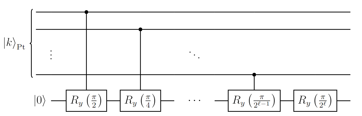
Figure 1: This circuit R is a controlled rotation

Next we perform a series of controlled rotations $R$ (circuit in Figure 1) of the form

$$R\ket{k}\ket{0}:=\ket{k}\left(\sqrt{1-t^{\prime}_{\ell}(k)}\ket{0}+\sqrt{t^{\prime}_{\ell}(k)}\ket{1}\right),$$

Where $t^{\prime}_{\ell}(k)=t_{\ell+1}(2k+1)$ will be used to sample the height of the $k^{\text{th}}$ subinterval in the Darboux sum. $t^{\prime}_{\ell}(k)$ is always somewhere in the range $[t_{\ell}(k),t_{\ell}(k+1)]$. R is then performed on each qubit in the player register controlled by the partition register. In total, these applications of R can be performed with $O(n\log n)$ gates in $O(n)$ layers and yield the state:

$$\ket{\psi_{2}}=\sum\limits_{k=0}^{2^{\ell}-1}\sqrt{w_{\ell}(k)}\ket{k}_{\text{Pt}}\left(\sqrt{1-t_{\ell}(k)}\ket{0}+\sqrt{t_{\ell}(k)}\ket{1}\right)^{\otimes n}\ket{0}_{\text{Ut}}.$$

Note that the player register is of size n. Let $H_{m}$ be the set of binary numbers of hamming distance $m$ from $0$ in $n$ bits, then we can rewrite $\ket{\psi_{2}}$ as:

$$\ket{\psi_{2}}=\sum\limits_{k=0}^{2^{\ell}-1}\sqrt{w_{\ell}(k)}\ket{k}_{\text{Pt}}\sum\limits_{m=0}^{n}\sqrt{t_{\ell}(k)^{m}(1-t_{\ell}(k))^{n-m}}\sum\limits_{h\in H_{m}}\ket{h}_{\text{Pl}}\ket{0}_{\text{Ut}}.$$

Example 1.

For a concrete example of this change, consider $n=2$, then

$$\left(\sqrt{1-t_{\ell}(k)}\ket{0}+\sqrt{t_{\ell}(k)}\ket{1}\right)^{\otimes 2}= \sqrt{(1-t_{\ell}(k))^{2}}\ket{00}+\sqrt{t_{\ell}(k)(1-t_{\ell}(k))}\ket{01}$$

$$+\sqrt{t_{\ell}(k)(1-t_{\ell}(k))}\ket{10}+\sqrt{t_{\ell}(k)^{2}}\ket{11}$$

Note that $\ket{00}$ is hamming distance $0$ from $\ket{00}$, $\ket{01}$ and $\ket{10}$ are hamming distance $1$ from $\ket{00}$, and $\ket{11}$ is hamming distance $2$ from $\ket{00}$. With this knowledge in hand, we can rewrite our state as,

$$\sqrt{(1-t_{\ell}(k))^{2}}\sum\limits_{h\in H_{0}}\ket{h}+\sqrt{t_{\ell}(k)(1-t_{\ell}(k))}\sum\limits_{h\in H_{1}}\ket{h}+\sqrt{t_{\ell}(k)^{2}}\sum\limits_{h\in H_{2}}\ket{h}$$

This can now be arranged into the desired form,

$$\sum\limits_{m}^{n}\sqrt{t_{\ell}(k)^{m}(1-t_{\ell}(k))^{n-m}}\sum\limits_{h\in H_{m}}\ket{h}$$

Rearranging $\ket{\psi_{2}}$ gives,

$$\ket{\psi_{2}}=\sum\limits_{m=0}^{n}\sum\limits_{h\in H_{m}}\sum\limits_{k=0}^{2^{\ell}-1}\sqrt{w_{\ell}(k)t_{\ell}(k)^{m}(1-t_{\ell}(k))^{n-m}}\ket{k}_{\text{Pt}}\ket{h}_{\text{Pl}}\ket{0}_{\text{Ut}}.$$

Next, we can take $U_{V}^{-}$ and $U_{V}^{+}$. Note that we take these separately on separate runs of the algorithm, and then compare the statistics of the two approaches. For convenience, let us for the moment write $U^{\pm}_{V}\ket{h}\ket{0}=\ket{h}\ket{V^{\pm}(h)}$, where,

$$\ket{V^{\pm}(h)}=\sqrt{\frac{1-\hat{V}^{\pm}(h)}{2}}\ket{0}+\sqrt{\frac{1+\hat{V}^{\pm}(h)}{2}}\ket{1}$$

Applying $U_{V}^{\pm}\ket{h}_{\text{Pl}}\ket{0}_{\text{Ut}}$ gives $\ket{\psi_{3}^{\pm}}$ is equal to,

$$\sum\limits_{m=0}^{n}\sum\limits_{h\in H_{m}}\sum\limits_{k=0}^{2^{\ell}-1}\sqrt{w_{\ell}(k)t_{\ell}(k)^{m}(1-t_{\ell}(k))^{n-m}}\ket{k}_{\text{Pt}}\ket{h}_{\text{Pl}}\ket{V^{\pm}(h)}_{\text{Ut}}.$$

This operation is wholly dependent on the game or algorithm being analyzed and its complexity. Assuming the algorithm is being implemented with a look up table, one could likely use qRAM giovannetti2008quantum . This approach would have a time complexity of $O(n)$ at the cost of requiring $O(2^{n})$ qubits for storage. However, depending on the problem, there will often be far less resource intense methods of implementing $U_{V}$, as will be seen with the voting game example in a later section.

This is the final quantum state. Let us now analyze this state through the lens of density matrices. Taking the partial trace with respect to the partition and player registers yields,

$$\tr_{\text{Pt},\text{Pl}}(\outerproduct{\psi_{3}^{\pm}}{\psi_{3}^{\pm}})= \sum\limits_{m=0}^{n}\sum\limits_{h\in H_{m}}\left(\sum\limits_{k=0}^{2^{\ell}-1}w_{\ell}(k)t_{\ell}(k)^{m}(1-t_{\ell}(k))^{n-m}\right)$$

$$\ket{V^{\pm}(h)}_{\text{Ut}}\bra{V^{\pm}(h)}_{\text{Ut}}.$$

It will be shown later in this work that,

$$\sum\limits_{k=0}^{2^{\ell}-1}w_{\ell}(k)t_{\ell}(k)^{m}(1-t_{\ell}(k))^{n-m}\approx\gamma(n,m)$$

with an error inversely proportional to $2^{\ell}$. Intuitively, this can be thought of as a Darboux sum approximation of a slightly modified beta function. This modified beta function happens to be exactly equal to $\gamma(n,m)$. The specifics of the error will be discussed in further detail and proved in later sections. As a result,

$$\tr_{\text{Pt},\text{Pl}}(\outerproduct{\psi_{3}^{\pm}}{\psi_{3}^{\pm}})\approx\sum\limits_{m=0}^{n}\sum\limits_{h\in H_{m}}\gamma(n,m)\ket{V^{\pm}(h)}_{\text{Ut}}\bra{V^{\pm}(h)}_{\text{Ut}}.$$

Finally, we measure the qubit in the utility register in the computational basis yields the following expected value.

$$\sum\limits_{m=0}^{n}\sum\limits_{h\in H_{m}}\gamma(n,m)\frac{1+\hat{V}^{\pm}(h)}{2}$$

Which is equal to

$$\frac{1}{2}\sum\limits_{m=0}^{n}\sum\limits_{h\in H_{m}}\gamma(n,m)\hat{V}^{\pm}(h)+\frac{1}{2}\sum\limits_{m=0}^{n}\sum\limits_{h\in H_{m}}\gamma(n,m)$$

With the ability to craft these plus and minus states we can now extract the required information to find a close approximation to the Shapley value. Note that it is necessary to extract the expected values for the utility register of both our plus and minus states. This is achieved by repeatedly constructing state $\ket{\psi_{3}^{+}}$ in the case of the plus state and constructing state $\ket{\psi_{3}^{-}}$ in the case of the minus state. Respectively one would measure repeatedly measure the utility register of these states, creating binomial distributions of $\ket{0}$ and $\ket{1}$ measurements. From these binomial distributions it is possible to find the underlying probability, in addition, it is possible to construct a confidence interval wallis2013binomial . This estimation of the expected values will take up the bulk of the runtime for the algorithm.

By first subtracting the expected result of the minus expected value from the positive expected value, then simplifying we get an expected value of:

$$\frac{1}{2}\sum\limits_{m=0}^{n}\sum\limits_{h\in H_{m}}\gamma(n,m)\left(\hat{V}^{+}(h)-\hat{V}^{-}(h)\right)$$

Plugging in the definition for $\hat{V}^{\pm}(h)$ gives

$$\frac{1}{2\cdot V_{\text{max}}}\sum\limits_{m=0}^{n}\sum\limits_{h\in H_{m}}\gamma(n,m)\left(V\left(S_{h}\cup\{i\}\right)-V\left(S_{h}\right)\right)$$

Notice that, in the $S_{x}$ encoding, $H_{m}$ represents each subset of $F\setminus\{i\}$ of size $m$. As a result, the equation is, in effect, summing over each subset of $F\setminus\{i\}$. Combining this observation with a final step of multiplying by $2\cdot V_{m}ax$, yields:

$$\sum\limits_{S\subseteq F\setminus\{i\}}\gamma(\lvert F\setminus\{i\}\rvert,\lvert S\rvert)\cdot\left(V\left(S\cup\{i\}\right)-V\left(S\right)\right).$$

This is precisely the Shapley value $\Phi_{i}$.

4 Our Proposal

4.1 Shapley Values and the Beta Function

In this subsection, the relationship between the beta function and Shapley values is explored.

Given a game with a set of $F$ players, a subset $S\subseteq F$, and a player $i$, we have,

Definition 4.

Let $n=\lvert F\setminus\{i\}\rvert$, and $m=\lvert S\rvert$. We denote the weights used to calculate the Shapley value in the weighted average as:

$$\gamma(n,m)=\frac{m!(n-m)!}{(n+1)!}=\frac{1}{{n\choose m}(n+1)}$$

Definition 5.

Denote a function closely related to the beta function as:

$$B_{\alpha,\beta}=\int\limits_{0}^{1}x^{\beta}(1-x)^{\alpha-\beta}dx,\quad 0\leq\beta\leq\alpha,\quad\alpha,\beta\in\mathbb{N}.$$

We will refer to this function as the special beta function. We also denote,

$$b_{\alpha,\beta}(x)=x^{\beta}(1-x)^{\alpha-\beta}$$

So that $B_{\alpha,\beta}=\int_{0}^{1}b_{\alpha,\beta}(x)dx$.

Lemma 1.

We have the following recurrence relationship:

$$B_{\alpha,\beta}=\frac{\beta}{\alpha-(\beta-1)}B_{\alpha,\beta-1}$$

$$B_{\alpha,0}=B_{\alpha,\alpha}=\frac{1}{\alpha+1}$$

Proof: Case 1, $\beta=0\text{ or }\alpha$:

$$B_{\alpha,0}=\int\limits_{0}^{1}(1-x)^{\alpha}dx=-\frac{(1-x)^{\alpha+1}}{\alpha+1}\bigg{\rvert}_{0}^{1}=\frac{1}{\alpha+1}$$

a nearly identical calculation can be used to show $B_{\alpha,\alpha}=\frac{1}{\alpha+1}$.

Case 2, $0<\beta<\alpha$:

$$B_{\alpha,\beta} =\int\limits_{0}^{1}x^{\beta}(1-x)^{\alpha-\beta}dx$$

$$=\frac{x^{\beta}(1-x)^{\alpha-(\beta-1)}}{\alpha-(\beta-1)}\bigg{\rvert}_{0}^{1}-\int\limits_{0}^{1}\frac{-\beta}{\alpha-(\beta-1)}x^{\beta-1}(1-x)^{\alpha-(\beta-1)}dx$$

$$=0+\frac{\beta}{\alpha-(\beta-1)}\int\limits_{0}^{1}x^{\beta-1}(1-x)^{\alpha-(\beta-1)}dx$$

$$=\frac{\beta}{\alpha-(\beta-1)}B_{\alpha,\beta-1}$$

Theorem 2.

The $B$ function is equivalent to the Shapley weight function $\gamma$:

$$B_{n,m}=\gamma(n,m),\quad 0\leq m\leq n,\quad m,n\in\mathbb{N}$$

Proof: Fix $n$, we proceed by induction.

Base case, $m=0$: then $B_{n,0}=\frac{1}{n+1}=\gamma(n,0)$, thus the base case holds.

Inductive step: suppose $B_{n,k}=\gamma(n,k)$, $k\in\mathbb{N}$, we need to show $B_{n,k+1}=\gamma(n,k+1)$, $0\leq k<\alpha$:

$$B_{n,k+1} =\frac{k+1}{n-k}B_{n}(k)$$

$$=\frac{k+1}{n-k}\gamma(n,k)$$

$$=\frac{k+1}{n-k}\cdot\frac{k!(n-k)!}{(n+1)!}$$

$$=\frac{(k+1)!(n-(k+1))!}{(n+1)!}$$

$$=\gamma(n,k+1)$$

To summarize, we have shown that our formulation of the beta function is equivalent to the Shapely value weight function over our domain.

4.2 Approximating the Special Beta Function

In this section, we will be going through the task of showing that we can approximate the beta function using fairly unusual partitions. Though it may not be immediately obvious, our partition definition is extremely convenient for a quantum implementation. For the moment, it is sufficient to understand this section as pursuing a single goal: showing that our partition can be used to approximate the area under $b_{n,m}$ over range $[0,1]$, which is equal to the special beta function. In fact, we will show that we can estimate $B_{n,m}$ with arbitrary accuracy.

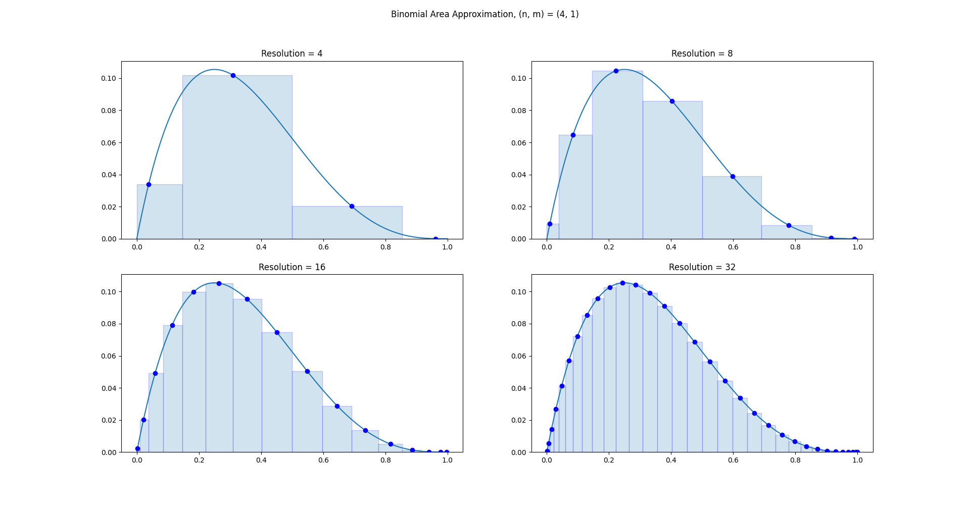
Figure 2: Visual representation of the special beta function being approximated using Darboux integrals and our novel partition.

For a visual representation of our goal, we will be estimating the area under $b_{n,m}$ over range $[0,1]$ using our strange partition for a Darboux integral as can be seen with various resolutions in Figure 2.

4.2.1 Partition

To begin, we consider a simple function, which, as we will see in later parts, is extremely natural in the quantum context.

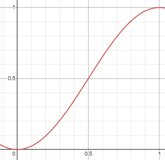
Figure 3: Graph of function $\sin^{2}\left(\frac{\pi}{2}x\right)$.

Remark 1.

Consider the following function from the real numbers in the range $0\leq x\leq 1$ to the reals such that:

$$\sin^{2}\left(\frac{\pi}{2}x\right)$$ (1)

As can be seen in Figure 3, $\sin^{2}\left(\frac{\pi}{2}x\right)$ is clearly monotonic and bijective from the domain $[0,1]$ to the range $[0,1]$.

Definition 6.

Let $\ell$ be an non-negative integer, and let $P_{\ell}=\left(t_{\ell}(0),t_{\ell}(1),\dots,t_{\ell}(2^{\ell}-1),t_{\ell}(2^{\ell})\right)$ be a partition of the interval $[0,1]$ where,

$$t_{\ell}(k)=\sin^{2}\left(\frac{\pi}{2}\cdot\frac{k}{2^{\ell}}\right)$$

Note that $t_{\ell}(x)$ can be interpreted as a discretized version of the function in Remark 1, where instead of $x\in[0,1]$, we have $x\in\left\{\frac{k}{2^{\ell}}:k=0,\dots,2^{\ell}\right\}\subset[0,1]$ for some fixed $\ell$.

Remark 2.

$P_{\ell+1}$ is a refinement of $P_{\ell}$.

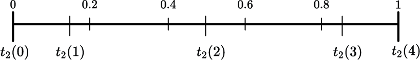
Figure 4: Visualization of Partition $P_{\ell}$, $\ell=2$.

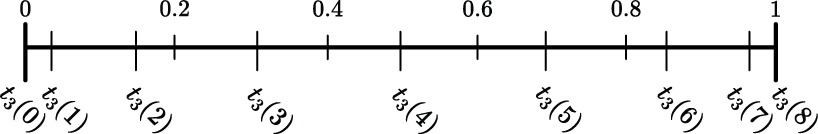
Figure 5: Visualization of Partition $P_{\ell}$, $\ell=3$.

Example 2.

In Figures 4 and 5, we can see concrete examples of how $t_{\ell}(k)$ partitions the interval $[0,1]$. Note that $P_{3}$ has a point corresponding to each point in $P_{2}$. Specifically,

$$t_{2}(i)=t_{3}(2i),\quad i\in\mathbb{N}$$

This behaviour is due to the aforementioned refinement relationship between $P_{\ell}$ and $P_{\ell+1}$. It is also worth noting how $P_{3}$’s intervals can be viewed as the intervals in $P_{2}$ split in two.

Lemma 3.

We have the following properties for the function $t_{\ell}(k)$:

1. This represents a kind of symmetry with respect to $k=2^{\ell-1}$

   $$t_{\ell}(k)=1-t_{\ell}\left(2^{\ell}-k\right)$$

2. $$t_{\ell}(k)=t_{\ell+1}(2k)$$

Proof: Property 1:

$$t_{\ell}(2^{\ell}-k) =\sin^{2}\left(\frac{\pi}{2}\cdot\left(\frac{2^{\ell}-k}{2^{\ell}}\right)\right)$$

$$=\sin^{2}\left(\frac{\pi}{2}\cdot\left(1-\frac{k}{2^{\ell}}\right)\right)$$

$$=\sin^{2}\left(\frac{\pi}{2}\cdot\left(-\frac{k}{2^{\ell}}\right)+\frac{\pi}{2}\right)$$

$$=\cos^{2}\left(\frac{\pi}{2}\cdot\left(-\frac{k}{2^{\ell}}\right)\right) \left(\cos(x)=\sin\left(x+\frac{\pi}{2}\right)\right)$$

$$=\cos^{2}\left(\frac{\pi}{2}\cdot\frac{k}{2^{\ell}}\right) \big{(}\cos(x)=\cos(-x)\big{)}$$

$$=1-\sin^{2}\left(\frac{\pi}{2}\cdot\frac{k}{2^{\ell}}\right) \big{(}\cos^{2}(x)=1-\sin^{2}(x)\big{)}$$

$$=1-t_{\ell}(k)$$

Property 2:

$$t_{\ell+1}(2k)=\sin{{}^{2}\left(\frac{\pi}{2}\cdot\frac{2k}{2^{\ell+1}}\right)}=\sin{{}^{2}\left(\frac{\pi}{2}\cdot\frac{k}{2^{\ell}}\right)}=t_{\ell}(k)$$

It will be useful to define a width for each sub-interval $\left[t_{\ell}(k),t_{\ell}(k+1)\right]$.

Definition 7.

Denote the width of a sub-interval $\left[t_{\ell}(k),t_{\ell}(k+1)\right]$ in a partition $P_{\ell}$ as:

$$w_{\ell}(k)=t_{\ell}(k+1)-t_{\ell}(k)$$

$w_{\ell}(k)$ can be interpreted as a function from $k\in\mathbb{N}$, $0\leq k\leq 2^{\ell}-1$, to $\mathbb{R}$. This width varies with respect to both $k$ and $\ell$, where $\ell$ increasing decreases $w_{\ell}(k)$, and middling values of $k$ maximize $w_{\ell}(k)$ as is apparent in Figures 2 and 6.

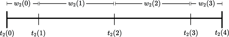
Figure 6: Visualization of $w_{2}(k)$, $k=0,1,2,3$ over partition $P_{2}$

Example 3.

In Figure 6, we can see a visual representation of $w_{2}(k)$ for $k=0,1,2,3$.

When refining our partition from $P_{\ell}$ to $P_{\ell+1}$, each sub-interval, $\left[t_{\ell}(k),t_{\ell}(k+1)\right]$, is split into two, $\left[t_{\ell+1}(2k),t_{\ell+1}(2k+1)\right]$ and $\left[t_{\ell+1}(2k+1),t_{\ell+1}(2k+2)\right]$ (recall, by lemma 3 property 2, $t_{\ell}(k)=t_{\ell+1}(2k)$). The relative sizes between the original sub-interval and the new ones are of critical importance.

Definition 8.

The previous-to-new-left-interval-ratio $\rho$ is defined as:

$$\rho_{\ell-1}(k)=\frac{w_{\ell}(2k)}{w_{\ell}(2k)+w_{\ell}(2k+1)}$$

$\rho_{\ell-1}(k)$ can also be interpreted as a function with $k\in\mathbb{N}$, $0\leq k\leq 2^{\ell}-1$

$\rho_{\ell-1}(k)$ represents how the sizes of intervals are modified during a refinement from $P_{\ell-1}$ to $P_{\ell}$.

Remark 3.

The previous-to-new-left-interval-ratio $\rho$ can equivalently be represented as:

$$\rho_{\ell-1}(k)=\frac{t_{\ell}(2k+1)-t_{\ell}(2k)}{t_{\ell}(2k+2)-t_{\ell}(2k)}=\frac{w_{\ell}(2k)}{w_{\ell-l}(k)}$$

Example 4.

Let us consider $P_{1}$ equal to the partition $(0,0.5,1)$. When we refine to $P_{2}$, the first interval, $\text{interval}_{\text{old}}=[0,0.5]$ of $P_{1}$ is split into two new intervals, $\text{interval}_{\text{left}}=[0,0.15]$ and $\text{interval}_{\text{right}}=[0.15,0.5]$ (note that $\text{interval}_{\text{old}}=\text{interval}_{\text{left}}\cup\text{interval}_{\text{right}}$). Consequently, the previous-to-new-left-interval-ratio $\rho_{1}(0)$ is equal to $\frac{w_{2}(0)}{w_{2}(0)+w_{2}(1)}$ which is approximately $0.3$, see Figure 6. $\rho_{1}(0)$ represents the relative size of the new left interval, $\text{interval}_{\text{left}}=[0,0.15]$ compared to the old interval ${interval}_{\text{old}}=[0,0.5]$.

Corollary 3.1.

The first partition refinement $P_{0}\to P_{1}$ splits the interval in two parts, which happen to be equal sizes.

$$\rho_{0}(0)=\frac{1}{2}$$

This can be verified easily though basic calculation.

Lemma 4.

As our partition approaches infinite density, the leftmost interval $[0,b]$ is split into two pieces, $[0,a]$ and $[a,b]$, $a$ approaches $\frac{b}{4}$. Equivalently,

$$\lim_{\ell\to\infty}\rho_{\ell-1}(0)=\frac{1}{4}$$

Proof:

$$\lim_{\ell\to\infty}\rho_{\ell-1}(0) =\lim_{\ell\to\infty}\frac{t_{\ell}(1)-t_{\ell}(0)}{t_{\ell}(2)-t_{\ell}(0)}=\lim_{\ell\to\infty}\frac{\sin^{2}\left(\frac{\pi}{2}\cdot\frac{1}{2^{\ell}}\right)}{\sin^{2}\left(\frac{\pi}{2}\cdot\frac{2}{2^{\ell}}\right)}=\lim_{\ell\to\infty}\frac{\left(\frac{\pi}{2}\cdot\frac{1}{2^{\ell}}\right)^{2}}{\left(\frac{\pi}{2}\cdot\frac{2}{2^{\ell}}\right)^{2}}=\frac{1}{4}$$

Lemma 5.

$\rho_{\ell}(0)$ monotonically decreases as $\ell$ increases, for $\ell\geq 0$.

Proof: Let $x=\frac{2}{\pi}2^{\ell}$. Then,

$$\rho_{\ell-1}(0) =\frac{t_{1}^{\ell}-t_{0}^{\ell}}{t_{2}^{\ell}-t_{0}^{\ell}}=\frac{\sin^{2}\left(\frac{\pi}{2}\cdot\frac{1}{2^{\ell}}\right)-\sin^{2}(0)}{\sin^{2}\left(\frac{\pi}{2}\cdot\frac{2}{2^{\ell}}\right)-\sin^{2}(0)}=\frac{\sin^{2}(\frac{1}{x})}{\sin^{2}(\frac{2}{x})}$$

Define $h(x)=\frac{sin^{2}\left(\frac{1}{x}\right)}{sin^{2}\left(\frac{2}{x}\right)}$, $x\in\left[\frac{2}{\pi},\infty\right)$, our result will hold if $h(x)$ decreases monotonically as $x$ increases over its domain. This is true when $\frac{d}{dx}h(x)<0$. We have,

$$\frac{d}{dx}h(x)=-\frac{2\sin\left(\frac{1}{x}\right)\left(\cos\left(\frac{1}{x}\right)\sin\left(\frac{2}{x}\right)-2\sin\left(\frac{1}{x}\right)\cos\left(\frac{2}{x}\right)\right)}{\sin^{3}\left(\frac{2}{x}\right)x^{2}}$$

Note that for $x\geq\frac{2}{\pi}$:

$$\frac{2\sin\left(\frac{1}{2x}\right)}{\sin^{3}\left(\frac{2}{x}\right)x^{2}}>0$$

Thus, $\frac{d}{dx}h(x)<0$ when,

$$\cos\frac{1}{x}\sin\frac{2}{x}-2\sin\frac{1}{x}\cos\frac{2}{x}>0$$

We can continue as follows, using the double angle identities:

$$\cos\frac{1}{x}\sin\frac{2}{x}-2\sin\frac{1}{x}\cos\frac{2}{x} =\cos\frac{1}{x}\left(2\sin\frac{1}{x}\cos\frac{1}{x}\right)-2\sin\frac{1}{x}\left(\cos^{2}\frac{1}{x}-1\right)$$

$$=2\sin\frac{1}{x}\cos^{2}\frac{1}{x}-2\sin\frac{1}{x}\cos^{2}\frac{1}{x}+2\sin\frac{1}{x}$$

$$=2\sin\frac{1}{x}$$

$$>0$$

This is trivially true for $x\geq\frac{2}{\pi}$. Hence, $\frac{d}{dx}h(x)<0$. As a result $\rho_{\ell}(0)$ monotonically decreases when $\ell$ increases.

Corollary 5.1.

By lemma 3.1, $\rho_{0}(0)=\frac{1}{2}$, and by lemma 4 $\lim_{\ell\to\infty}\rho_{\ell}(0)=\frac{1}{4}$. Thus, since $\rho_{\ell}(0)$ is monotonically decreasing with respect to $\ell$ (lemma 5), it is clear that $\rho_{\ell}(0)\in\left(\frac{1}{4},\frac{1}{2}\right]$

Lemma 6.

Similarly, we have $\rho_{\ell}(2^{\ell}-1)\in\left[\frac{1}{2},\frac{3}{4}\right)$.

Proof: Let us begin by showing:

$$\rho_{\ell}(2^{\ell}-1)=1-\rho_{\ell}(0)$$

Plugging in $2^{\ell}-1$,

$$\rho_{\ell}(2^{\ell}-1) =\frac{t_{\ell}(2^{\ell}-1)-t_{\ell}(2^{\ell}-2)}{t_{\ell}(2^{\ell})-t_{\ell}(2^{\ell}-2)}$$

$$=\frac{(1-t_{\ell}(1))-(1-t_{\ell}(2))}{1-(1-t_{\ell}(2))} \left(\text{Lemma~{}\ref{lemma:tProperties}, Property }2\right)$$

$$=\frac{t_{\ell}(2)-t_{\ell}(1)}{t_{\ell}(2)}$$

$$=1-\frac{t_{\ell}(1)}{t_{\ell}(2)}$$

$$=1-\rho_{\ell}(0)$$

As was shown in corollary 5.1, $\rho_{\ell}(0)\in\left(\frac{1}{4},\frac{1}{2}\right]$, thus $\rho_{\ell}(2^{\ell}-1)\in\left[\frac{1}{2},\frac{3}{4}\right)$.

So we have figured out the bounds of $\rho_{\ell}$ for the extreme values of its domain. The next step will be to show that $\rho_{\ell}(k)<\rho_{\ell}(k+1)$ for all valid k. This will give us a chain of inequalities, which will bound all $\rho$.

Lemma 7.

The following statement relates an inequality of weights to an inequality of previous-to-new-left-interval-ratios:

$$\frac{w_{\ell}(2k)}{w_{\ell}(2k+1)}<\frac{w_{\ell}(2k+2)}{w_{\ell}(2k+3)}\iff\rho_{\ell-1}(k)<\rho_{\ell-1}(k+1)$$

Proof: Applying some basic algebra,

$$\frac{w_{\ell}(2k)}{w_{\ell}(2k+1)}<\frac{w_{\ell}(2k+2)}{w_{\ell}(2k+3)}\iff w_{\ell}(2k)w_{\ell}(2k+3)<w_{\ell}(2k+2)w_{\ell}(2k+1)$$

Adding $w_{\ell}(2k)w_{\ell}(2k+2)$ ($>0$ by remark 4) to both sides results in,

$$w_{\ell}(2k)w_{\ell}(2k+2)+w_{\ell}(2k)w_{\ell}(2k+3)<w_{\ell}(2k)w_{\ell}(2k+2)+w_{\ell}(2k+2)w_{\ell}(2k+1)$$

Which can be factored into,

$$w_{\ell}(2k)(w_{\ell}(2k+2)+w_{\ell}(2k+3))<w_{\ell}(2k+2)(w_{\ell}(2k)+w_{\ell}(2k+1))$$

Rearranging gives,

$$\frac{w_{\ell}(2k)}{w_{\ell}(2k)+w_{\ell}(2k+1)}<\frac{w_{\ell}(2k+2)}{w_{\ell}(2k+2)+w_{\ell}(2k+3)}$$ (2)

Finally, by definition of previous-to-new-left-interval-ratio $\rho$,

$$\rho_{\ell}(k)<\rho_{\ell}(k+1)$$

This relation will be helpful in showing $\rho_{\ell-1}(k)<\rho_{\ell-1}(k+1)$, as $w_{\ell}$ is an easier function to manage.

Definition 9.

Fix $\ell$, let us define the following real number extensions of $t_{\ell}$, $T(x)$ and $w_{\ell}$, $W(x)$. Where the domains and codomains of $T(x)$ and $W(x)$ are $\mathbb{R}$.

$$T(x)=\sin^{2}\left(\frac{\pi}{2}\cdot\frac{x}{2^{\ell}}\right)$$

and,

$$W(x)=T(x+1)-T(x)$$

where $x\in[0,2^{\ell}-1]$ is real.

Corollary 7.1.

Fix $\ell$. If $k\in\mathbb{N}$, $0\leq k\leq 2^{\ell}$, then $T(k)=t_{\ell}(k)$, and $W(k)=w_{\ell}(k)$.

With $w_{\ell}$ and $t_{\ell}$ extended to the real numbers, it is possible to apply tools from calculus, making the next few proofs substantially easier.

Remark 4.

Clearly, $T(x)$ increases as $x$ increases. As a result $W(x)>0$ for $x\in[0,2^{\ell}-1]$.

Remark 5.

With the new function $W$, it is possible to extend the expression seen in lemma 7,

$$\frac{W(x)}{W(x+1)}<\frac{W(x+2)}{W(x+3)},\quad x\in\left[0,2^{\ell}-1\right]$$

With corollary 7.1 in mind, it is easy to see that if this relation holds in this extended context, then it will also hold for the relation with $w_{\ell}$.

Remark 6.

The relation can be simplified further by considering,

$$\frac{W(x)}{W(x+1)}<\frac{W(x+1)}{W(x+2)}$$

Assuming this holds for all $x$, it is very obvious that,

$$\frac{W(x)}{W(x+1)}<\frac{W(x+1)}{W(x+2)}\Rightarrow\frac{W(x)}{W(x+1)}<\frac{W(x+2)}{W(x+3)}$$

So proving $\frac{W(x)}{W(x+1)}<\frac{W(x+1)}{W(x+2)}$, will be sufficient to show $\rho_{\ell}(k)<\rho_{\ell}(k+1)$.

Lemma 8.

Fix $\ell$. The derivative of W(x) is greater than the derivative of W(x+1):

$$\frac{d}{dx}W(x)>\frac{d}{dx}W(x+1)\quad x\in\left[0,2^{\ell}-1\right]$$

Proof: We first find $\frac{d}{dx}W(x+r)$, for an arbitrary $r\in\mathbb{R}$.

$$\frac{d}{dx}T(x+r) =\frac{d}{dx}\sin^{2}\left(\frac{\pi}{2}\left(\frac{x+r}{2^{\ell}}\right)\right)$$

$$=\frac{d}{dx}\sin^{2}\left(\frac{\alpha}{2}(x+r)\right) \left(\alpha=\frac{\pi}{2^{L}}\right)$$

$$=\alpha\sin(\alpha(x+r))$$

Thus, we have $\frac{d}{dx}W(x+r)$:

$$\frac{d}{dx}W(x+r) =\frac{d}{dx}T(x+r+1)-\frac{d}{dx}T(x+r)$$

$$=\alpha\big{(}\sin(\alpha(x+r+1))-\sin(\alpha(x+r))\big{)}$$

Finally, we show:

$$\frac{d}{dx}W(x)>\frac{d}{dx}W(x+1) \iff\alpha(\sin(\alpha(x+1))-\sin(\alpha x)))$$

$$\quad>\alpha(\sin(\alpha(x+2))-\sin(\alpha(x+1)))$$

$$\iff 2\sin(\alpha(x+1))-\sin(\alpha x)-\sin(\alpha(x+2))>0$$

Let $u=\alpha x$, $v=\alpha$ then,

$$2\sin(u+v)-\sin(u)-\sin(u+2v) =2(\sin u\cos v+\cos u\sin v)-\sin u$$

$$\quad-(\sin u\cos 2v+\cos u\sin 2v)$$

$$=2\sin u\cos v+2\cos u\sin v-\sin u$$

$$\quad-\sin u(2\cos^{2}v-1)-\cos u(2\sin v\cos v)$$

$$=2\sin u\cos v+2\cos u\sin v-\sin u$$

$$\quad-2\sin u\cos^{2}v+\sin u-2\sin v\cos^{2}v$$

$$=2\sin u\cos v(1-\cos v)+2\cos u\sin v(1-\cos v)$$

$$=2(\sin u\cos v+\cos u\sin v)(1-\cos v)$$

$$=2\sin(u+v)(1-\cos v)$$

$$=2\sin(\alpha x+\alpha)(1-\cos\alpha)$$

$$=2\sin\left(\pi\cdot\frac{x+1}{2^{\ell}}\right)\left(1-\cos\frac{\pi}{2^{\ell}}\right)$$

It is easily shown that $1-\cos\frac{\pi}{2^{\ell}}>0$ for $\ell\geq 0$, thus, the result holds when:

$$\sin\left(\pi\frac{x+1}{2^{\ell}}\right)>0$$

This is equivalent to when $0<\frac{x+1}{2^{\ell}}<1$. Hence,

$$\frac{d}{dx}W(x)>\frac{d}{dx}W(x+1),\quad\text{if }x\in[0,2^{L}-1]$$

Lemma 9.

In the real domain, the ratio of the previous width to the current width increases monotonically, that is,

$$\frac{W(x)}{W(x+1)}<\frac{W(x+1)}{W(x+2)},\quad x=\left[0,2^{\ell}-1\right].$$

Proof: By lemma 8, the derivative of current width $W^{\prime}(x+1)$ is lower than the derivative of the previous width $W^{\prime}(x)$. This implies that,

$$\int_{x+1}^{x+2}W^{\prime}(z)dz<\int_{x}^{x+1}W^{\prime}(z)dz.$$

Let $\Delta W(x)$ be equal to $\int_{x}^{x+1}W^{\prime}(z)dz$. Since $W(x)>0$ (see Remark 4), multiplying both sides by W(x), it is apparent that $W(x)\Delta W(x+1)$ is less than $W(x)\Delta W(x)$. Adding $W(x)^{2}+W(x)\Delta W(x)$ to both sides and $\Delta W(x)^{2}$ (which is $>0$) to the right hand side shows that $W(x)^{2}+W(x)\Delta W(x)+W(x)\Delta W(x+1)$ is less than $W(x)^{2}+2W(x)\Delta W(x)+\Delta W(x)^{2}$. Factoring gives,

$$W(x)\left[W(x)+\Delta W(x)+\Delta W(x+1)\right]<(W(x)+\Delta W(x))^{2}$$

Note that $W(x)+\Delta W(x)$ is equal to $\int_{0}^{x}W^{\prime}(z)dz+\int_{x}^{x+1}W^{\prime}(z)dz$ which is equal to $\int_{0}^{x+1}W^{\prime}(z)dz$. By a similar argument it can shown that $W(x)+\Delta W(x)+\Delta W(x+1)$ is equal to $\int_{0}^{x+2}W^{\prime}(z)dz$. Hence, it follows that,

$$W(x)\int_{0}^{x+2}W^{\prime}(z)dz<\left(\int_{0}^{x+1}W^{\prime}(z)dz\right)^{2}.$$

By the fundamental theorem of calculus, $W(x)W(x+2)$ is less than $W(x+1)^{2}$. Rearranging yields,

$$\frac{W(x)}{W(x+1)}<\frac{W(x+1)}{W(x+2)}.$$

Corollary 9.1.

The following relation holds, $\rho_{\ell}(k)<\rho_{\ell}(k+1)$ for all $k\in[0,2^{\ell}-2]$.

Proof: This is a direct result of Lemmas 7 and 9.

Theorem 10.

For all $\ell,k\in\mathbb{N}$, $0\leq k\leq 2^{\ell}-1$, $\rho_{\ell}(k)$ is bounded with,

$$\rho_{\ell}(k)\in\left[\frac{1}{4}+\epsilon,\frac{3}{4}-\epsilon\right],\quad\epsilon>0$$

Proof: By Corollary 5.1 we have $\rho_{\ell}(0)\in\left[\frac{1}{4}+\epsilon,\frac{1}{2}\right]$, thus $\rho_{\ell}(0)>\frac{1}{4}$. By Lemma 6 we have $\rho_{\ell}(2^{\ell}-1)\in\left[\frac{1}{2},\frac{3}{4}-\epsilon\right]$, so $\rho_{\ell}(2^{\ell}-1)<\frac{3}{4}$. Finally, by Corollary 9.1, we have $\rho_{\ell}(k)<\rho_{\ell}(k+1)$ for the current range of $k=0,\dots,2^{\ell}-1$. This results in the following chain of inequalities:

$$\frac{1}{4}<\rho_{\ell}(0)<\rho_{\ell}(1)<\cdots<\rho_{\ell}\left(2^{\ell}-1\right)<\frac{3}{4}$$

4.2.2 Area Estimation

Various important properties about the partitioning scheme $P_{\ell}$ have been the primary focus. This section focuses on estimating the area under $b_{n,m}$ given a partition $P_{\ell}$, using concepts from Darboux integrals. The end goal is to show that error can become arbitrarily small given a large enough $\ell$. This section also lays the foundations for a better, and more realistic upper bound for error in estimating Shapley values, which is covered in a later section.

Definition 10.

The supremum of a set $S\subseteq\mathbb{R}$ is,

$$\sup(S)=\min\limits_{x\in\mathbb{R}}x\geq s,\quad\forall s\in S.$$

The infimum of $S$ is,

$$\inf(S)=\max\limits_{x\in\mathbb{R}}x\leq s,\quad\forall s\in S.$$

Definition 11.

Darboux sums takes a partition $P=(z_{0},z_{1},\dots,z_{n})$ of an interval $[a,b]$, where $a=z_{0}<z_{1}<\cdots<z_{n}=b$, and a function $f$ which maps $(a,b)$ to $\mathbb{R}$. Each interval $\left[z_{i},z_{i+1}\right]$ is called a subinterval. Let

$$M_{i}=\sup\limits_{x\in[z_{i},z_{i+1}]}f(x),\quad\text{and}\quad m_{i}=\inf\limits_{x\in[z_{i},z_{i+1}]}f(x),\quad i=0,\ldots,n-1$$

The upper and lower bounds of a sub interval’s area are,

$$A_{U}(f,[z_{i},z_{i+1}])=(z_{i+1}-z_{i})M_{i},\quad and\quad A_{L}(f,[z_{i},z_{i+1}])=(z_{i+1}-z_{i})m_{i}$$

respectively. The upper Darboux sum is:

$$U(f,P)=\sum\limits_{i=0}^{n-1}A_{U}(f,[z_{i},z_{i+1}]),$$

and the lower Darboux sum is:

$$L(f,P)=\sum\limits_{i=0}^{n-1}A_{L}(f,[z_{i},z_{i+1}]),$$

There is a geometric interpretation of the Darboux sums. Each subinterval has a rectangle width corresponding to the subinterval witch, and a height corresponding to either the supremum or infimum of $f(x)$. The upper Darboux sum is the sum of the areas of these rectangles, where their heights correspond to their suprema.

Remark 7.

Suppose instead of taking $M_{i}$ or $m_{i}$, we took arbitrary elements from each subinterval to represent the heights of the rectangles:

$$\sum\limits_{i=0}^{n-1}(z_{i+1}+z_{i})f(x_{i})\quad x_{i}\in[z_{i},z_{i+1}].$$ (3)

By definitions of supremum and infimum (Definition 10), it is clear that for all $i=0,\ldots,n-1$, $m_{i}\leq x_{i}\leq M_{i}$. It follows that for all $i$, the areas $A_{L}(f,[z_{i},z_{i+1}])$ are less than or equal to the areas $(z_{i+1}-z_{i})f(x_{i})$ which are less than or equal to the areas $A_{U}(f,[z_{i},z_{i+1}])$. This gives,

$$L(f,P)\leq\sum\limits_{i=0}^{n-1}(z_{i+1}+z_{i})f(x_{i})\leq U(f,P).$$

As a result, there is a lot of freedom in choosing which part of the subinterval to assess $f(x)$

Lemma 11.

For any subinterval $[z_{i},z_{i+1}]$, and function $f$ that maps elements of $[z_{i},z_{i+1}]$ to $\mathbb{R}$,

$$A_{L}(f,[z_{i},z_{i+1}])\leq\int\limits_{z_{i}}^{z_{i+1}}f(x)dx\leq A_{U}(f,[z_{i},z_{i+1}])$$

Proof: Consider $A_{L}(f,[z_{i},z_{i+1}])$ which is equal to $(z_{i+1}-z_{i})m_{i}$ where $m_{i}$ is equal to $\inf_{x\in[z_{i},z_{i+1}]}f(x)$. Note that,

$$(z_{i+1}-z_{i})m_{i}=\int\limits_{z_{i}}^{z_{i+1}}m_{i}dx.$$

By Definition 10, for all $x\in[z_{i},z_{i+1}]$, $f(x)$ greater or equal to $m_{i}$. Thus,

$$\int\limits_{z_{i}}^{z_{i+1}}f(x)dx\geq\int\limits_{z_{i}}^{z_{i+1}}m_{i}dx=A_{L}(f,[z_{i},z_{i+1}]).$$

A nearly identical argument can be used to show $\int_{z_{i}}^{z_{i+1}}f(x)dx\leq A_{U}(f,[z_{i},z_{i+1}])$.

The next lemma bounds the error resulting from estimating the area under a subinterval by picking a random point on that subinterval and making a rectangle.

Lemma 12.

Take an arbitrary point $y$ in the subinterval $[z_{i},z_{i+1}]$, then,

$$\left\lvert\int\limits_{z_{i}}^{z_{i+1}}f(x)dx-(z_{i+1}-z_{i})f(y)\right\rvert\leq A_{U}(f,[z_{i},z_{i+1}])-A_{L}(f,[z_{i},z_{i+1}])$$

Proof: Recall that by Definition 11 $A_{L}(f,[z_{i},z_{i+1}])$ is equal to $(z_{i+1}-z_{i})m_{i}$, and $A_{U}(f,[z_{i},z_{i+1}])$ is equal to $(z_{i+1}-z_{i})M_{i}$, where,

$$m_{i} =\inf\limits_{x\in[z_{i},z_{i+1}]}f(x),\quad and$$

$$M_{i} =\sup\limits_{x\in[z_{i},z_{i+1}]}f(x).$$

By Definition 10, $m_{i}\leq f(y)\leq M_{i}$, which implies $A_{L}(f,[z_{i},z_{i+1}])\leq(z_{i+1}-z_{i})f(y)\leq A_{U}(f,[z_{i},z_{i+1}])$. Let us assume $(z_{i+1}-z_{i})f(y)$ be less than or equal to $\int_{z_{i}}^{z_{i+1}}f(x)dx$, meaning $\left\lvert\int\limits_{z_{i}}^{z_{i+1}}f(x)dx-(z_{i+1}-z_{i})f(y)\right\rvert$ is equal to $\int\limits_{z_{i}}^{z_{i+1}}f(x)dx~{}-~{}(z_{i+1}-z_{i})f(y)$. Then, since Lemma 11 shows $\int_{z_{i}}^{z_{i+1}}f(x)dx\leq A_{U}(f,[z_{i},z_{i+1}])$, it follows that

$$\int\limits_{z_{i}}^{z_{i+1}}f(x)dx-(z_{i+1}-z_{i})f(y)\leq A_{U}(f,[z_{i},z_{i+1}])-(z_{i+1}-z_{i})f(y).$$

As shown above, it is also the case that $(z_{i+1}-z_{i})f(y)$ is greater than or equal to $A_{L}(f,[z_{i},z_{i+1}])$. As a result,

$$A_{U}(f,[z_{i},z_{i+1}])-(z_{i+1}-z_{i})f(y)\leq A_{U}(f,[z_{i},z_{i+1}])-A_{L}(f,[z_{i},z_{i+1}]).$$

With similar argumentation, we can show this also holds for $(z_{i+1}-z_{i})f(y)$ is greater than or equal to $\int_{z_{i}}^{z_{i+1}}f(x)dx$.

Remark 8.

Consider the following approach to approximating area under $f$ on the interval $[z_{i},z_{i+1}]$: choose an arbitrary $x\in[z_{i},z_{i+1}]$, multiply by width of interval. Clearly, in this context, the error is equal to $\left\lvert(z_{i+1}-z_{i})f(x)-\int_{z_{i}}^{z_{i+1}}f(x)dx\right\rvert$. By Lemma 12, it follows that $A_{U}(f,[z_{i},z_{i+1}])-A_{L}(f,[z_{i},z_{i+1}])$ can be used as an upper bound for error when using this this approach.

Corollary 12.1.

Given a partition $P_{\ell}=\left(t_{\ell}(0),\dots,t_{\ell}\left({2^{\ell}}\right)\right)$, the upper bound of error when approximating area under $b_{n,m}(x)$ over the $k^{th}$ subinterval is defined as:

$$UE_{n,m}(\ell,k)=\left(t_{\ell}(k+1)-t_{\ell}(k)\right)\Big{[}U(b_{n,m},[t_{\ell}(k),t_{\ell}(k+1)])-L(b_{n,m},[t_{\ell}(k),t_{\ell}(k+1)])\Big{]}$$

Remark 9.

Note that $b_{n,m}(x)$ has at most one local maximum for $x\in[0,1]$, for all valid $n,m$. As a result, given a partition $P$ of $[0,1]$, on every subinterval of $P$ (except when the subinterval contains the local maximum, which occurs in only one subinterval), $b_{n,m}(x)$ is either monotonically increasing or decreasing. For each subinterval $[z_{i},z_{i+1}]$ of $P$ on which $b_{n,m}(x)$ is monotonically increasing, $L(b_{n,m},[z_{i},z_{i+1}])$ is equal to $b_{n,m}(z_{i})$ and $U(b_{n,m},[z_{i},z_{i+1}])$ is equal to $b_{n,m}(z_{i+1})$. When $b_{n,m}(x)$ is decreasing over $[z_{i},z_{i+1}]$, $L(b_{n,m},[z_{i},z_{i+1}])$ is equal to $b_{n,m}(z_{i+1})$ and $U(b_{n,m},[z_{i},z_{i+1}])$ is equal to $b_{n,m}(z_{i})$.

Corollary 12.2.

Given a partition $P_{\ell}=\left(t_{\ell}(0),\dots,t_{\ell}\left({2^{\ell}}\right)\right)$, the following monotonic-assumption upper bound of error when approximating the area under $b_{n,m}(x)$ over the $k^{th}$ subinterval is defined as:

$$\overline{UE}_{n,m}(\ell,k)=\left(t_{\ell}(k+1)-t_{\ell}(k)\right)\big{\lvert}b_{n,m}(t_{\ell}(k+1))-b_{n,m}(t_{\ell}(k))\big{\rvert}$$

This definition makes easy finding an error upper bound for all intervals except one, the one containing the local maximum.

Corollary 12.3.

If $b_{n,m}(x)$ is monotonic over $[t_{\ell}(k),t_{\ell}(k+1)]$, then $UE_{n,m}(\ell,k)$ is equal to $\overline{UE}_{n,m}(\ell,k)$.

Lemma 13.

Let us suppose a partition $P_{\ell-1}$ is refined to partition $P_{\ell}$. Given a subinterval $[t_{\ell-1}(k),t_{\ell-1}(k+1)]$ of $P_{\ell}$, the monotonic-assumption upper bound of error is reduced over that interval by a factor of at least $3/4$, that is:

$$\frac{3\cdot\overline{UE}_{n,m}(\ell-1,k)}{4}>\left(\overline{UE}_{n,m}(\ell,2k)+\overline{UE}_{n,m}(\ell,2k+1)\right)$$

Proof:

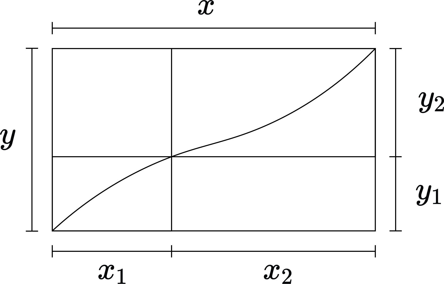
Figure 7: Example visualization of $\overline{UE}_{n,e}$’s change during refinement for arbitrary function.

Let us consider Figure 7, there are the following widths,

$$x=t_{\ell-1}(k+1)-t_{\ell-1}(k),\quad y=\left\lvert b_{n,m}(t_{\ell-1}(k+1))-b_{n,m}(t_{\ell-1}(k))\right\rvert,\\$$

where $x$ and $y$ represent the width and change in height of the previous subinterval. Also there are the following widths,

$$x_{1}=t_{\ell}(2k+1)-t_{\ell}(2k),\quad y_{1}=\left\lvert b_{n,m}(t_{\ell}(2k+1))-b_{n,m}(t_{\ell}(2k))\right\rvert,\\$$

where $x_{1}$ and $y_{1}$ represent the width and change in height of the left part of split previous subinterval. It follows that the width and change in height of the right part of the split subinterval have values,

$$x_{2}=x-x_{1},\quad y_{2}=y-y_{1}.$$

It is concluded that,

$$\overline{UE}_{n,m}(\ell-1,k) =x\cdot y,$$

$$\overline{UE}_{n,m}(\ell,2k) =x_{1}\cdot y_{1},\text{ and}$$

$$\overline{UE}_{n,m}(\ell,2k+1) =x_{2}\cdot y_{2}.$$

Finally, let us define $\overline{x}=\frac{x_{1}}{x}$, and $\overline{y}=\frac{y_{1}}{y}$. Note that when considering $\overline{UE}_{n,m}(\ell-1,k)$,

$$\overline{x}=\frac{x_{1}}{x}=\frac{t_{\ell}(2k+1)-t_{\ell}(2k)}{t_{\ell}(2k+2)-t_{\ell}(2k)}=\rho_{\ell-1}(k),$$

by Remark 3. Thus by Theorem 10, $\frac{1}{4}<\overline{x}<\frac{3}{4}$. Simultaneously, $0\leq\overline{y}\leq 1$. We proceed by simplifying the following expression

$$\frac{\overline{UE}_{n,m}(\ell,2k)+\overline{UE}_{n,m}(\ell,2k+1)}{\overline{UE}_{n,m}(\ell-1,k)}=\frac{x_{1}y_{1}+x_{2}y_{2}}{xy}$$

Plugging in the definition for $x_{2}$ and $y_{2}$, the above is equivalent to,

$$\frac{x_{1}y_{1}+(x-x_{1})(y-y_{1})}{xy}$$

Doing the product and applying the definitions for $\overline{x}$ and $\overline{y}$ yields

$$2\overline{x}\>\overline{y}-\overline{y}-\overline{x}+1.$$

Rearranging, it can be shown that the above is equal to

$$2\left(\overline{x}-\frac{1}{2}\right)\left(\overline{y}-\frac{1}{2}\right)+\frac{1}{2}.$$

Let us assume that $\left(\overline{y}-1/2\right)$ is positive without loss of generality. Then assigning to $\overline{x}$ and $\overline{y}$ their respective maximum values, the following inequality is obtained,

$$\frac{\overline{UE}_{n,m}(\ell,2k)+\overline{UE}_{n,m}(\ell,2k+1)}{\overline{UE}_{n,m}(\ell-1,k)}<2\left(\frac{3}{4}-\frac{1}{2}\right)\left(1-\frac{1}{2}\right)+\frac{1}{2}=\frac{3}{4}$$

A similar argument can be used for when $\left(\overline{y}-1/2\right)$ is negative, and the above is trivially correct for $\left(\overline{y}-1/2\right)$ equals zero.

Corollary 13.1.

For all monotonic sub-intervals $\left[t_{\ell}(k),t_{\ell}(k+1)\right]$, the upper bound of error $UE_{n,m}(\ell,k)$ is reduced by at least $25\%$ when the partition is refined from $P_{\ell}$ to $P_{\ell+1}$.

Proof: This follows as a direct result of Lemma 13.

Next, let us consider error over the whole of the approximation.

Definition 12.

We denote the sum of upper bounds for error over all sub-intervals as:

$$SUE_{n,m}(\ell)=\sum\limits_{k=0}^{2^{\ell}-1}UE_{n,m}(\ell,k),$$

and the sum of upper bounds for error over all sub-intervals with the monotonic assumption for all sub-intervals as:

$$\overline{SUE}_{n,m}(\ell)=\sum\limits_{k=0}^{2^{\ell}-1}\overline{UE}_{n,m}(\ell,k).$$

To discuss how error evolves with respect to granularity of our partition, having an upper bound for initial error is critical.

Definition 13.

We denote initial error as,

$$\sigma_{n,m}=SUE_{n,m}(0)$$

Remark 10.

Using the first and second derivative tests, one can verify that $b_{n,m}(m/n)$ is the supremum of $b_{n,m}(x)$ for $x\in[0,1]$. One can also easily show the infimum of $b_{n,m}(x)$ is $0$. Thus,

$$\sigma_{n,m}=SUE_{n,m}(0)=UE_{n,m}(0,0)=b_{n,m}\left(\frac{m}{n}\right)$$

Lemma 14.

$$\overline{SUE}_{n,m}(\ell+1)\leq\frac{3}{4}\overline{SUE}_{n,m}(\ell)$$

Proof: By Definition 12,

$$\overline{SUE}_{n,m}(\ell+1)=\sum\limits_{k=0}^{2^{\ell+1}-1}\overline{UE}_{n,m}(\ell+1,k).$$

Rearranging the values in the sum yields,

$$\overline{SUE}_{n,m}(\ell+1)=\sum\limits_{k=0}^{2^{\ell}-1}\left[\overline{UE}_{n,m}(\ell+1,2k)+\overline{UE}_{n,m}(\ell+1,2k+1)\right].$$

Hence by Lemma 13,

$$\overline{SUE}_{n,m}(\ell+1)<\sum\limits_{k=0}^{2^{\ell}-1}\left[\frac{3}{4}\overline{UE}_{n,m}(\ell,k)\right]\\ =\frac{3}{4}\overline{SUE}_{n,m}(\ell).$$

5 Example

5.1 Games

5.1.1 Voting Games

To begin, we define a weighted voting game matsui2001np as follows:

Definition 14.

Consider a game G=(F, V), $F=\{1,2,\dots,N\}$, where each player $i$ has voting power $w_{i}\geq 0$, and the total votes need to sum to be greater or equal to a threshold $q$. Given a subset $S\subseteq F$, we have:

$$V(S)=\begin{cases}1&\quad\text{if }\sum\limits_{i\in S}w_{i}\geq q\\ 0&\quad\text{otherwise}\end{cases}$$

We denote this game as a weighted voting game.

The circuit implementation for this game (cf. Figure 8) is quite intuitive so long as each weight $w_{i}$ can be represented as a fixed point number, where $\ket{Votes},\ket{Out}$ are initialized to $\ket{0}$, and $\ket{Voters_{S}}=\ket{x_{0}x_{1}\cdots x_{N}}$ with,

$$x_{i}=\begin{cases}1&\quad\text{if }i\in S\\ 0&\quad\text{otherwise}\end{cases}$$

and

$$\geq(x,q)=\begin{cases}1&\quad\text{if }x\geq q\\ 0&\quad\text{otherwise}\end{cases}$$

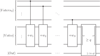
Figure 8: Circuit implementation for the weighted voting game.

For our particular example we will simplify this circuit even further. Suppose we have a three player weighted voting game with $w_{1}=3,w_{2}=2,w_{3}=1$ with $q=4$. One benefit of this voting game is given 3 bits to store the votes, instead of using the $\geq q$ circuit we can simply check the most significant qubit (as it will be flipped in any situation where the threshold has been passed).

We can work out the Shapley values by hand:

$$V(\emptyset) =0 \quad V(\{1,2\}) =1$$

$$V(\{1\}) =0 \quad V(\{1,3\}) =1$$

$$V(\{2\}) =0 \quad V(\{2,3\}) =0$$

$$V(\{3\}) =0 \quad V(\{1,2,3\}) =1$$

From this we have:

$$\Phi_{1} =\sum\limits_{S\subseteq F\setminus\{i\}}\sigma(\lvert F\setminus\{i\}\rvert,\lvert S\rvert)\cdot(V(S\cup\{i\})-V(S))$$

$$=\sigma(2,0)\cdot(V(1)-V(\{\emptyset\}))+\sigma(2,1)\cdot(V(\{1,2\})-V(\{2\}))$$

$$\quad+\sigma(2,1)\cdot(V(\{1,3\})-V(\{3\}))+\sigma(2,2)\cdot(V(\{1,2,3\})-V(\{2,3\}))$$

$$=\sigma(2,0)\cdot(0-0)+\sigma(2,1)\cdot(1-0)+\sigma(2,1)\cdot(1-0)+\sigma(2,2)\cdot(1-0)$$

$$=2\cdot\sigma(2,1)+\sigma(2,2)$$

$$=2\cdot\frac{1!(2-1)!}{(2+1)!}+\frac{2!(2-2)!}{(2+1)!}$$

$$=2\cdot\frac{1}{6}+\frac{1}{3}$$

$$=\frac{2}{3}$$

This can be repeated to get,

$$\Phi_{2},\Phi_{3}=\frac{1}{6}$$

5.1.2 Random Games

Though it is a common assumption in the literature, our framework works with non-superadditive contexts. This is because the equation Shapley derived for Shapley values did not rely on the assumption of superadditivity shapley1952value

6 Conclusion

We have addressed the context of quantum AI algorithms for supporting decision-making processes. In such a context, the problem of explainability is amplified, since measuring a quantum system destroys the information. The use of the classical concept of Shapley values for post-hoc explanations in quantum computing does not translate trivially. We have proposed a nove algorithm which reduces the problem of accurately estimating the Shapley values of a quantum algorithm into a far simpler problem of estimating the true average of a binomial distribution in polynomial time. We have determined the efficacy of the algorithm by using an analytic analysis. In our analysis, we have provided an upper bound of the error associated to the algorithm.

References

- \bibcommenthead
- (1) Goodman, B., Flaxman, S.: European Union regulations on algorithmic decision-making and a “right to explanation”. AI magazine 38(3), 50–57 (2017)
- (2) Rudin, C.: Stop explaining black box machine learning models for high stakes decisions and use interpretable models instead. Nature Machine Intelligence 1(5), 206–215 (2019)
- (3) Lundberg, S.M., Lee, S.-I.: A unified approach to interpreting model predictions. Advances in neural information processing systems 30 (2017)
- (4) Matsui, Y., Matsui, T.: NP-completeness for calculating power indices of weighted majority games. Theoretical Computer Science 263(1-2), 305–310 (2001)
- (5) Prasad, K., Kelly, J.S.: NP-completeness of some problems concerning voting games. International Journal of Game Theory 19(1), 1–9 (1990)
- (6) Castro, J., Gómez, D., Tejada, J.: Polynomial calculation of the Shapley value based on sampling. Computers & Operations Research 36(5), 1726–1730 (2009)
- (7) Biamonte, J., Wittek, P., Pancotti, N., Rebentrost, P., Wiebe, N., Lloyd, S.: Quantum machine learning. Nature 549(7671), 195–202 (2017)
- (8) Chen, S.Y.-C., Yang, C.-H.H., Qi, J., Chen, P.-Y., Ma, X., Goan, H.-S.: Variational quantum circuits for deep reinforcement learning. IEEE Access 8, 141007–141024 (2020)
- (9) Aumann, R.J.: Some non-superadditive games, and their Shapley values, in the Talmud. International Journal of Game Theory 39 (2010)
- (10) Winter, E.: The Shapley value. Handbook of game theory with economic applications 3, 2025–2054 (2002)
- (11) Hart, S.: Shapley value. In: Game Theory, pp. 210–216. Springer, (1989)
- (12) Shapley, L.S.: A Value for N-Person Games. RAND Corporation, Santa Monica, CA (1952). https://doi.org/10.7249/P0295
- (13) Lipovetsky, S., Conklin, M.: Analysis of regression in game theory approach. Applied Stochastic Models in Business and Industry 17(4), 319–330 (2001)
- (14) Van den Broeck, G., Lykov, A., Schleich, M., Suciu, D.: On the tractability of SHAP explanations. Journal of Artificial Intelligence Research 74, 851–886 (2022)
- (15) Bertossi, L., Li, J., Schleich, M., Suciu, D., Vagena, Z.: Causality-based explanation of classification outcomes. In: Proceedings of the Fourth International Workshop on Data Management for End-to-End Machine Learning, pp. 1–10 (2020)
- (16) Kulesza, T., Burnett, M., Wong, W.-K., Stumpf, S.: Principles of explanatory debugging to personalize interactive machine learning. In: Proceedings of the 20th International Conference on Intelligent User Interfaces, pp. 126–137 (2015)
- (17) Goebel, R., Chander, A., Holzinger, K., Lecue, F., Akata, Z., Stumpf, S., Kieseberg, P., Holzinger, A.: Explainable AI: the new 42? In: International Cross-domain Conference for Machine Learning and Knowledge Extraction, pp. 295–303 (2018). Springer
- (18) Hoffman, R.R., Mueller, S.T., Klein, G., Litman, J.: Metrics for explainable AI: Challenges and prospects. arXiv preprint arXiv:1812.04608 (2018)
- (19) Plesch, M., Brukner, Č.: Quantum-state preparation with universal gate decompositions. Physical Review A 83(3), 032302 (2011)
- (20) Giovannetti, V., Lloyd, S., Maccone, L.: Quantum random access memory. Physical review letters 100(16), 160501 (2008)
- (21) Wallis, S.: Binomial confidence intervals and contingency tests: mathematical fundamentals and the evaluation of alternative methods. Journal of Quantitative Linguistics 20(3), 178–208 (2013)