Two-Photon EXchange - TPEX

Abstract

We propose a new measurement of the ratio of positron-proton to electron-proton, elastic scattering at DESY to determine the contributions beyond single-photon exchange, which are essential to the QED description of the most fundamental process in hadronic physics. A 20 cm long liquid hydrogen target together with the extracted beam from the DESY synchrotron would yield an average luminosity of $2.12\times 10^{35}$ cm${}^{-2}\cdot$s${}^{-1}\cdot$sr^-1 ($\sim 200$ times the luminosity achieved by OLYMPUS). A commissioning run at 2 GeV followed by measurements at 3 GeV would provide new data up to $Q^{2}=4.6$ (GeV/$c$)² (twice the range of current measurements). Lead tungstate calorimeters would be used to detect the scattered leptons at polar angles of $30\degree$, $50\degree$, $70\degree$, $90\degree$, and $110\degree$. The measurements could be scheduled to not interfere with the operation of PETRA. We present rate estimates and simulations for the planned measurements including background considerations. Initial measurements at the DESY test beam facility using prototype lead tungstate calorimeters in 2019, 2021, and 2022 were made to check the Monte Carlo simulations and the performance of the calorimeters. These tests also investigated different readout schemes (triggered and streaming). Various upgrades are possible to shorten the running time and to make higher beam energies and thus greater $Q^{2}$ ranges accessible.

1 Introduction

Elastic lepton-proton scattering is a fundamental process that should be well described by QED. Understanding this interaction is important to the scientific programs at FAIR, Jefferson Lab, and the future electron-ion collider (EIC) planned for Brookhaven. It is described theoretically in the Standard Model by a perturbative expansion in $\alpha=\frac{1}{137}$ with radiative corrections. For more than half a century it has been assumed that the leading single-photon exchange term adequately describes the scattering process and that higher-order terms are negligible. However, recent experiments at Jefferson Lab have been widely interpreted as evidence that higher order terms are significant in elastic electron-proton scattering and must be included to correctly extract the proton elastic form factors. Recent experiments, including the OLYMPUS experiment at DESY, show little evidence for significant contributions beyond single photon exchange up to $Q^{2}\approx 2.3$ (GeV/c)². It is essential that the QED expansion be studied experimentally at higher $Q^{2}$ comparing the positron and electron scattering cross section to determine the contribution of higher order terms not normally included in radiative corrections.

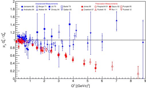
Figure 1: Proton form factor ratio measured using unpolarized [1, 2, 3, 4, 5, 6, 7, 8] (blue) and polarized [9, 10, 11, 12, 13, 14, 15, 16] (red) techniques.

The proton form factors, $G_{E}^{p}$ and $G_{M}^{p}$, have historically been envisaged as very similar and are often modeled by the same dipole form factor. Measurements over the past 50 years using the unpolarized Rosenbluth separation technique yielded a ratio, $\mu^{p}\,G_{E}^{p}/G_{M}^{p}$, close to unity over a broad range in $Q^{2}$ shown by the blue data points in Fig. 1. This supported the idea that $G_{E}^{p}$ and $G_{M}^{p}$ are similar. However, recent measurements using polarization techniques revealed a completely different picture with the ratio decreasing rapidly with increasing $Q^{2}$ as shown by the red data points in Fig. 1.

The most commonly proposed explanation for this discrepancy is “hard” two-photon exchange contributions beyond the standard radiative corrections to one-photon exchange.

Figure 2: Feynman diagrams for one- and two-photon exchange. Further diagrams for bremsstrahlung, vertex, self-energy, and vacuum polarization radiative corrections are not shown but must also be included in calculations.

Two-photon exchange, TPE, (see Fig. 2) is generally included as part of the radiative corrections when analyzing electron-proton scattering. However, it is usually only included in the “soft” limit where one of the two photons, in the diagrams with two photons, is assumed to carry negligible momentum and the intermediate hadronic state remains a proton. To include “hard” two-photon exchange, a model for the off-shell, intermediate hadronic state must also be included, making the calculations difficult and model dependent.

In the Born or single photon exchange approximation the elastic scattering cross section for leptons from protons is given by the reduced Rosenbluth cross section,

$$\frac{d\sigma_{e^{\pm}p}}{d\Omega}={\frac{d\sigma}{d\Omega}}_{Mott}\frac{\tau{G_{M}^{p}}^{2}+\epsilon{G_{E}^{p}}^{2}}{\epsilon(1+\tau)},$$ (1)

where: $\tau=\frac{Q^{2}}{4M_{p}^{2}}$ and $\epsilon=(1+2(1+\tau)\tan^{2}{\frac{\theta_{l}}{2}})^{-1}$.

To measure the “hard” two-photon contribution, one can measure the ratio $R_{2\gamma}=\sigma_{e^{+}p}/\sigma_{e^{-}p}$ at different values of $Q^{2}$ and $\epsilon$. Note, the interference terms between one- and two-photon exchange change sign between positron and electron scattering and this cross section ratio provides a measure of the two-photon exchange contribution.

The results from the OLYMPUS experiment [17] are shown in Fig. 3 together with various calculations.

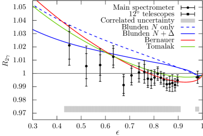
Figure 3: OLYMPUS results for $R_{2\gamma}$ as a function of $\epsilon$. Inner error bars are statistical while the outer error bars include uncorrelated systematic uncertainties added in quadrature. The gray band is correlated systematic uncertainty.

The deviation of the results from unity are small, on the order of 1%, and are below unity at large $\epsilon$ and rising with decreasing $\epsilon$. The dispersive calculations of Blunden [18] are systematically above the OLYMPUS results in this energy regime. The results below unity cannot be explained by current QED calculations. The phenomenological prediction from Bernauer [19] and the subtractive dispersion calculation from Tomalak [20] are in better agreement with the OLYMPUS results but appear to rise too quickly as $\epsilon$ decreases. There is some indication that TPE increases with decreasing $\epsilon$ or increasing $Q^{2}$, suggesting that a significant “hard” two-photon contribution might be present at lower $\epsilon$ or higher $Q^{2}$.

Two other experiments, VEPP-3 [21] and CLAS [22], also measured the “hard” two-photon exchange contribution to electron-proton elastic scattering.

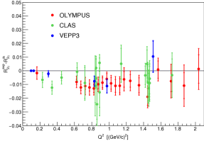
(a)

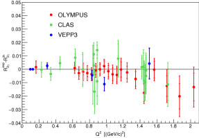
(b)

Figure 4: Difference between the results from the three recent experiments and (a) Blunden’s N+$\Delta$ calculation and (b) Bernauer’s prediction.

.

It is difficult to compare the results from the three experiments directly since the measurements are at different points in the $(\epsilon,Q^{2})$ plane. To partially account for this, we can compare all the two-photon exchange results by taking the difference with respect to a selected calculation evaluated at the correct $(\epsilon,Q^{2})$ for each data point. This is shown in Fig. 4a for Blunden’s calculation and in  Fig. 4b for Bernauer’s phenomenological prediction, plotted versus $Q^{2}$. In these views, the results from the three experiments are shown to be in reasonable agreement supporting the previous conclusions.

The results from the three TPE experiments are all below $Q^{2}=2.3$ (GeV/c)². In this regime the discrepancy in the form factor ratios is not obvious, so the small “hard” TPE contribution measured is consistent with the measured form factor ratios. The suggested slope with $\epsilon$ indicates TPE may be important at smaller $\epsilon$ or higher $Q^{2}$. But, since this slope appears to deviate from Bernauer’s phenomenological prediction, which fits the observed discrepancy, it may also suggest that “hard” TPE, while contributing, may not explain all of the observed form factor discrepancy.

Recently, the OLYMPUS data has also been analyzed to determine the charge-averaged yield for elastic lepton-proton scattering [23]. The result is shown in Fig. 5.

Figure 5: The charge-averaged yield for elastic lepton-proton scattering from the OLYMPUS experiment [23].

This measurement is insensitive to any charge-odd radiative corrections including “hard” two-photon exchange and thus provides a better measure of the proton form factors. The data shown covers an important range of $Q^{2}$ where the $G_{M}$ form factor changes slope. The calculations by Kelly [24] and Arrington [25, 26] appear to be in better agreement with the data, but Bernauer’s global fit [19] should be redone to incorporate all the OLYMPUS data.

The two-photon exchange diagram in the QED expansion for electron scattering is an example of the more generic electroweak photon-boson diagram (see Fig. 6 where $V=Z^{0},W^{\pm},{\rm or}\ \gamma$) which enters into a number of fundamental processes in subatomic physics. The $\gamma-Z$ box is a significant contribution to the asymmetry in parity-violating electron scattering and the $\gamma-W^{\pm}$ box is an important radiative correction in $\beta-$decay which must be implemented to extract $V_{ud}$ of the Standard Model from $0^{+}\rightarrow 0^{+}$ super-allowed nuclear $\beta$-decays. A workshop [27] was held at the Amherst Center for Fundamental Interactions in September 2017, attended by physicists from these different subfields, to discuss the Electroweak Box. A white paper is in preparation.

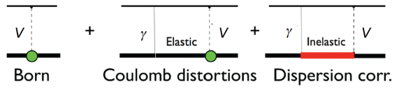
Figure 6: More general electroweak box diagram that is important in many fundamental nuclear physics processes.

The proton form factors are fundamental to hadronic physics. Understanding the QED expansion, the role of two-photon exchange, and the scale of radiative corrections at higher $Q^{2}$ will be crucial in future studies at FAIR, JLab, EIC, and elsewhere. The charge-averaged yield eliminates all charge-odd radiative corrections including the leading terms of two-photon exchange, which cannot be calculated with current theories. Measuring the ratio of positron-proton to electron-proton scattering is sensitive to the charge-odd radiative corrections and insensitive to the charge-even radiative corrections. Together they help to study radiative corrections and unravel the proton form factors. TPEX, like OLYMPUS, will provide both these measurements at higher $Q^{2}$.

The discrepancy in the form factor ratio has not been resolved and the role played by two-photon exchange continues to be widely discussed within the nuclear physics community [27, 28, 29, 30, 31]. Further measurements and theoretical work on the role of two-photon exchange on the proton form factors are clearly needed. However, measurements at higher $Q^{2}$ and smaller $\epsilon$, where the discrepancy is clear and TPE are expected to be larger, are difficult as the cross sections decrease rapidly. In addition, there are not many laboratories capable of providing both electron and positron beams with sufficient intensity.

The best, and for the foreseeable future only, opportunity is at DESY. This proposal outlines an experiment that could measure $R_{2\gamma}$ at $Q^{2}$ up to 4.6 (GeV/c)² or higher, and $\epsilon$ below 0.1 where the form factor discrepancy is clear (see Fig. 1). Such an experiment would overlap with the existing OLYMPUS data as a cross-check and would map out the two-photon exchange contribution over a broad range in $Q^{2}$ and $\epsilon$ to provide data to constrain theoretical calculations.

The following sections describe the proposed site for the TPEX experiment at DESY, the experimental configuration with its liquid hydrogen target, lead tungstate calorimeters, GEM detectors, luminosity monitor, beamdump/Faraday cup, electronics and data acquisition, and possible improvements. Sources of background are considered together with solutions and Monte Carlo simulations are presented. The appendices give more background plots, properties of hydrogen and lead tungstate, some useful numbers for this proposal, and references.

2 DESY

One of the primary requirements for measuring $R_{2\gamma}$ is high intensity positron and electron beams at energies of several GeV available for nuclear and particle physics applications. DESY is effectively the only high energy physics laboratory currently capable of such intense positron beams. The DESY II synchrotron can provide extracted beams of up to 30 nA of positrons and up to 60 nA of electrons at energies between 0.5 and 6.3 GeV with a bunch frequency of 12.5 Hz.

A proposal, currently under consideration at DESY for an extension to the present test beam facility [32], to include an extracted lepton beam from DESY II provides a unique opportunity to investigate two-photon exchange. The extracted beam would only be available when DESY-II is not needed for the operation of PETRA III. For our purposes the electron and positron beams would be used directly at 2.0 GeV and 3.0 GeV with an option for higher energies in the future.

The current operation of PETRA III uses only electrons. That would restrict the availability of positrons to times when PETRA III is not operating due to scheduled maintenance or shutdown periods. Hopefully this is not an insurmountable problem and we believe our experiment can be successfully carried out in the shutdown periods. Commissioning can be done with just electrons if necessary. If the storage ring PETRA III is running in “top up” mode (fills every $\sim 30$ s) we would not be able to run parasitically. For “non-top up” mode (fills every $\sim 240$ s) it might be possible to have the extracted beam for TPEX between fills for PETRA III.

If the modification to the test beam facility in Hall 2 provides a new, extracted beam area; this would allow a left/right symmetric detector arrangement that is much preferred for this proposal to reduce systematics and to increase count rate.

This proposal requires a significant effort from DESY:

1. The positron production target has been removed. This would need to be reinstalled.

2. A new, extracted beam area would have to be assembled. Two options are possible:

   • Hall 2

     • The floor space is currently occupied by another group that would have to be relocated.

     • The “kicker” would have to be moved from its current location on DESY II to one suitable for providing beams to the new area.

     • The shielding wall around DESY II would have to be disassembled and reassembled with a beamline incorporated to the new area.

   • R-Weg

     • The transfer line previously used for DORIS would have to be re-established for a new experimental area.

     • A new area, possibly a specially designed experimental area would have to be developed.

3. For both options beamline elements (quadrupoles, steering magnets, vacuum pumps, valves, collimators, beam dump, etc.) would have to be found or produced and then installed.

4. The new extracted beam area would need shielding walls, infrastructure services like power and water, an access maze with interlocks, and a new counting hut.

5. Everything would need to be surveyed and aligned and then tests performed to satisfy all safety requirements.

In addition to enabling the TPEX experiment, an extracted beam facility at DESY would allow other experiments, detector development, and material studies to be performed. Another interesting experiment would be Deeply Virtual Compton Scattering, DVCS. This could also use the TPEX liquid hydrogen target and lead tungstate calorimeters but with a different configuration to allow the scattered lepton and recoil proton to be detected in coincidence. Other nuclear physics measurements could also benefit from comparing electron and positron scattering.

3 Proposed Experiment

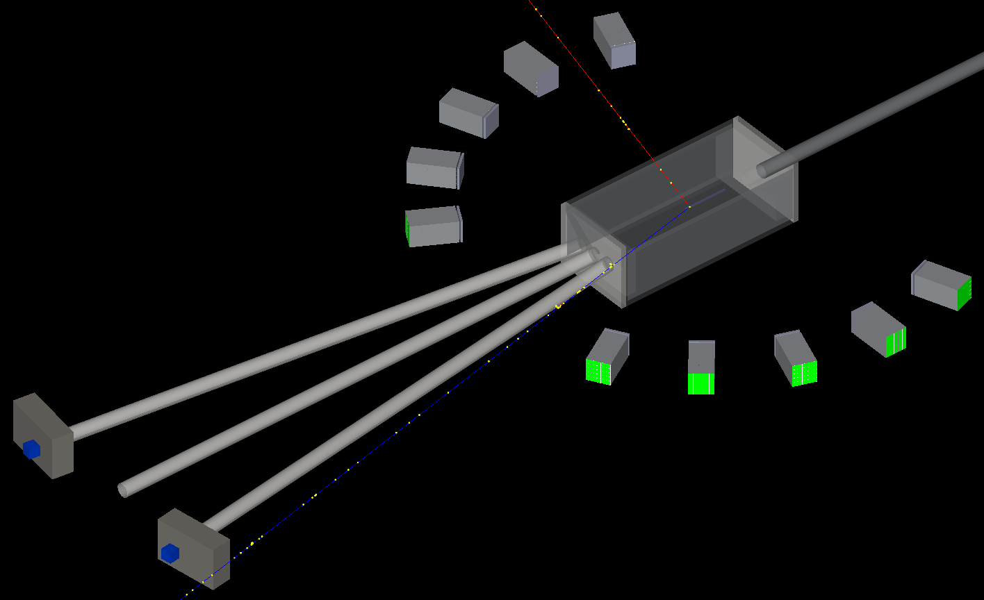
Figure 7: Geant4 simulation of a proposed TPEX target, scattering chamber, and detector configuration including the luminosity monitors and beamlines. The lepton beam would enter through the beamline in the upper-right, traverse the target cell, and scatter into the detectors or continue straight to the beamdump.

The proposed experimental configuration has ten $5\times 5$ arrays of lead tungstate crystals at polar angles of $30\degree$, $50\degree$, $70\degree$, $90\degree$, and $110\degree$ left and right of the beam axis with the front face of the calorimeter modules at a radius of 1 m from the target. Other configurations are possible and can be optimized with Monte Carlo studies. A simple schematic for this arrangement is shown in Fig. 7. The electron or positron beam enters the scattering chamber along the beamline (upper-right) and passes through the 20 cm long liquid hydrogen target before exiting the scattering chamber into another section of beam line leading to the beamdump. At $\pm 8\deg$ there are 3 m long beampipes connecting the scattering chamber to the lead collimators before the Cherenkov detectors used to monitor the luminosity. These beamlines are under vacuum and are used to reduce the multiple scattering for the relatively low energy (30–50 MeV) Møller and Bhabha scattered leptons.

Using just the central $3\times 3$ array of the $5\times 5$ array of crystals to define the acceptance yields a solid angle of 3.6 msr at each angle. With a 20 cm long liquid hydrogen target the acceptance covers $\pm 5.7\degree$ in polar and azimuthal angle thus data is averaged over a small range in $Q^{2}$ and $\epsilon$.

We propose to commission the experiment using 2 GeV electrons. We do this to debug the electronics, detectors, and data acquisition system taking advantage of the relatively high cross section at 2 GeV. We would require about 2 weeks of beam time for this commissioning after the experiment was installed and surveyed. We would also like a brief run (few days) with positrons to verify that the beam alignment and performance do not change with positron running. The commissioning run (including a few days with positrons) would also allow a crosscheck of the OLYMPUS data at $30\degree$, $50\degree$, and $70\degree$ and give a modest extension in $Q^{2}$ up to 2.7 (GeV/$c$)².

Table 1 shows $Q^{2}$, $\epsilon$, differential cross section, and event rate expected for one day of running for the proposed left/right symmetric configuration with 2 GeV lepton beams averaging 40 nA on a 20 cm liquid hydrogen target and using just the central $3\times 3$ array of crystals to calculate the acceptance area.

$\theta$	$Q^{2}$	$\epsilon$	$d\sigma/d\Omega$	Events/day
	(GeV/c)2		fb
$30\degree$	0.834	0.849	$2.41\times 10^{7}$	$3.16\times 10^{6}$
$50\degree$	1.62	0.611	$7.66\times 10^{5}$	$1.01\times 10^{5}$
$70\degree$	2.19	0.386	$1.00\times 10^{5}$	$1.32\times 10^{4}$
$90\degree$	2.55	0.224	$2.81\times 10^{4}$	$3.70\times 10^{3}$
$110\degree$	2.78	0.120	$1.22\times 10^{4}$	$1.61\times 10^{3}$

Table 1: Kinematics, cross section, and events expected in one day for an incident lepton beam of 2 GeV and 40 nA averaged current on a 20 cm liquid hydrogen target.

The TPEX experiment proper would run at 3.0 GeV and would require approximately 6 weeks (2 weeks with electrons and 4 weeks with positrons in total) to collect the required statistics. Table 2 shows $Q^{2}$, $\epsilon$, differential cross section, and event rate expected for one day of running for the proposed configuration with 3 GeV lepton beams. This would extend the measurements to $Q^{2}=4.57$ (GeV/$c$)² where the form factor ratio discrepancy is large. The 6 weeks could be divided into two three-week periods if that was more convenient. To minimize systematic we would like to switch between positron and electron running as frequently as possible (e.g. 1 day positron, 1 day electron, and 1 day positron repeating).

$\theta$	$Q^{2}$	$\epsilon$	$d\sigma/d\Omega$	Events/day
	(GeV/c)2		fb
$30\degree$	1.69	0.825	$2.41\times 10^{6}$	$3.16\times 10^{5}$
$50\degree$	3.00	0.554	$6.51\times 10^{4}$	$8.55\times 10^{3}$
$70\degree$	3.82	0.329	$8.94\times 10^{3}$	$1.17\times 10^{3}$
$90\degree$	4.29	0.184	$2.65\times 10^{3}$	$3.48\times 10^{2}$
$110\degree$	4.57	0.096	$1.20\times 10^{3}$	$1.58\times 10^{2}$

Table 2: Kinematics, cross section, and events expected in one day for an incident lepton beam of 3 GeV and 40 nA averaged current on a 20 cm liquid hydrogen target and 3.6 msr acceptance and a left/right symmetric detector configuration.

The $Q^{2}$ range that the proposed TPEX experiment would be capable of reaching is shown in Fig. 8 for the 2 and 3 GeV runs of this proposal. The reach with TPEX can be seen in relation to the discrepancy in the form factor ratio. With additional crystals at back angles the 4 GeV runs would also be possible in a reasonable time frame.

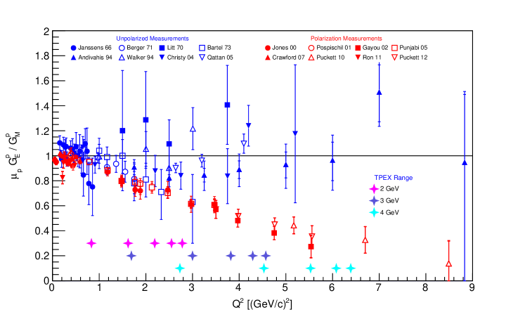
Figure 8: Proton form factor ratio as before but also showing the $Q^{2}$ range accessible with the proposed TPEX configuration at 2 and 3 GeV. The 4 GeV range would be possible with additional crystals.

The TPEX experiment at DESY would also measure the charge-averaged cross section just like the recent result from OLYMPUS Fig. 5. As mentioned above this cross section is insensitive to charge-odd radiative corrections including “hard” two-photon exchange terms. Thus, it provides a more robust measure of the proton form factors. The expected charge-averaged cross section uncertainties (assuming dipole cross section) are shown in Fig. 9 for TPEX assuming 6 days of running at 2 GeV and 6 weeks of running at 3 GeV with only 50% data collection efficiency. The recent OLYMPUS results are also shown.

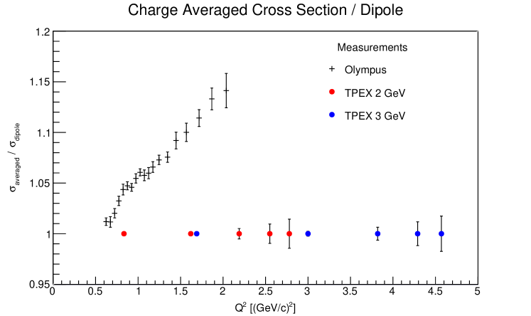
Figure 9: Charge-averaged cross section divided by the dipole cross section from OLYMPUS and expected uncertainties and coverage from TPEX at 2 and 3 GeV.

4 Liquid Hydrogen Target and Scattering Chamber

The OLYMPUS experiment that previously ran on the DORIS storage ring at DESY used an internal gas target with typical areal density of $3\times 10^{15}$ atoms$\cdot$cm^-2. The lepton current averaged around 60 mA, yielding an instantaneous luminosity about $1.12\times 10^{-6}$ fb${}^{-1}\cdot\,$s^-1.

For this new experiment we propose to build a liquid hydrogen target that will yield a luminosity about a factor of 200 times higher than that of the OLYMPUS experiment. This higher luminosity will greatly shorten the run time needed at 2 GeV and help to make up for the lower cross section at higher beam energies.

Table 3: Target system requirements.

Parameter	Performance Requirements
Liquid hydrogen	T$\approx$20 K and P$\geq$1 atm
Cool down time	$<$ 3 hrs.
Exit windows	scattering into $25\mathrm{°}$ – $120\mathrm{°}$ and $7\mathrm{°}$ – $9\mathrm{°}$ allowed
Target Cell	end cap wall thickness t${}_{c}\leq 0.5$ mm,
	inner diameter 10 mm $<$ i.d. $<$ 20 mm,
	wall thickness t${}_{w}\leq 1$ mm,
	20 cm in length

In order to satisfy the science needs for TPEX, and the safety requirements that always have to be taken into consideration for liquid hydrogen targets, we propose to build a liquid hydrogen target system that is tailored for this new experiment. The experimental requirements for the target system, detailed in Table 3, include a single, 20-cm long liquid hydrogen target with an areal density of $8.46\times 10^{23}$ atoms$\cdot$cm^-2 that can accommodate lepton currents up to 60 nA (30 nA for positrons and 60 nA for electrons); and long, thin scattering chamber windows to allow particles to be accepted over the large solid angle subtended by the detectors. Thus, the TPEX cryotarget system requires appropriate engineering and safety considerations. The Michigan group plans to work closely with the MIT-Bates engineers and an external company, Creare, Inc., to design and fabricate the system.

Figure 10 presents the conceptual design of the target system. Panel (a) shows a schematic overview of the target system, which consists of the scattering chamber, the cryo-cooler system, and the 20 cm long, and 2 cm wide single target cell. Details of the target system are shown in panels (b) and (c). In order to maximize rigidity and withstand the enormous force from atmospheric pressure, as well as to avoid welded and bolted joints, we propose to machine the scattering chamber from a single piece of aluminum.

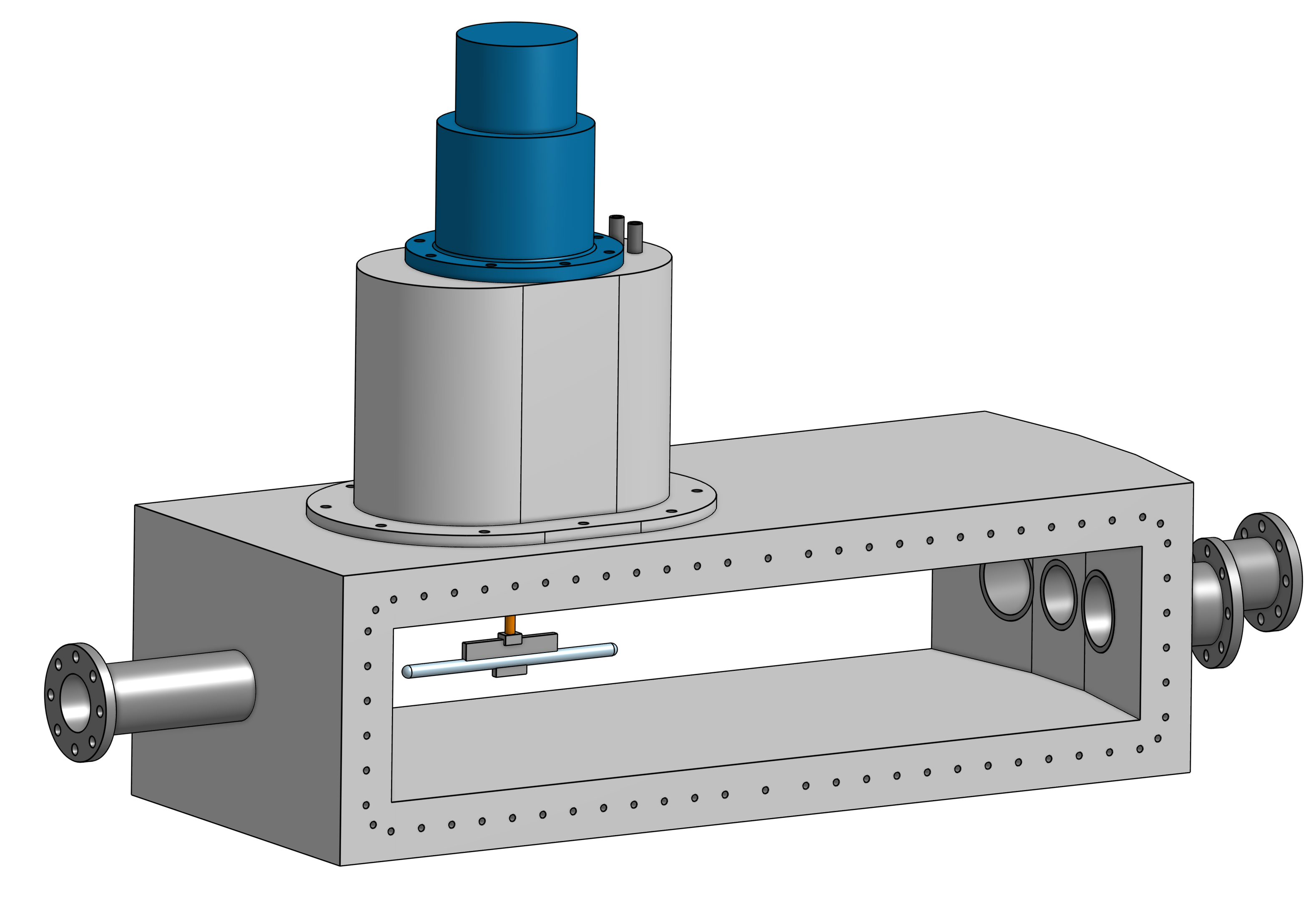
(a)

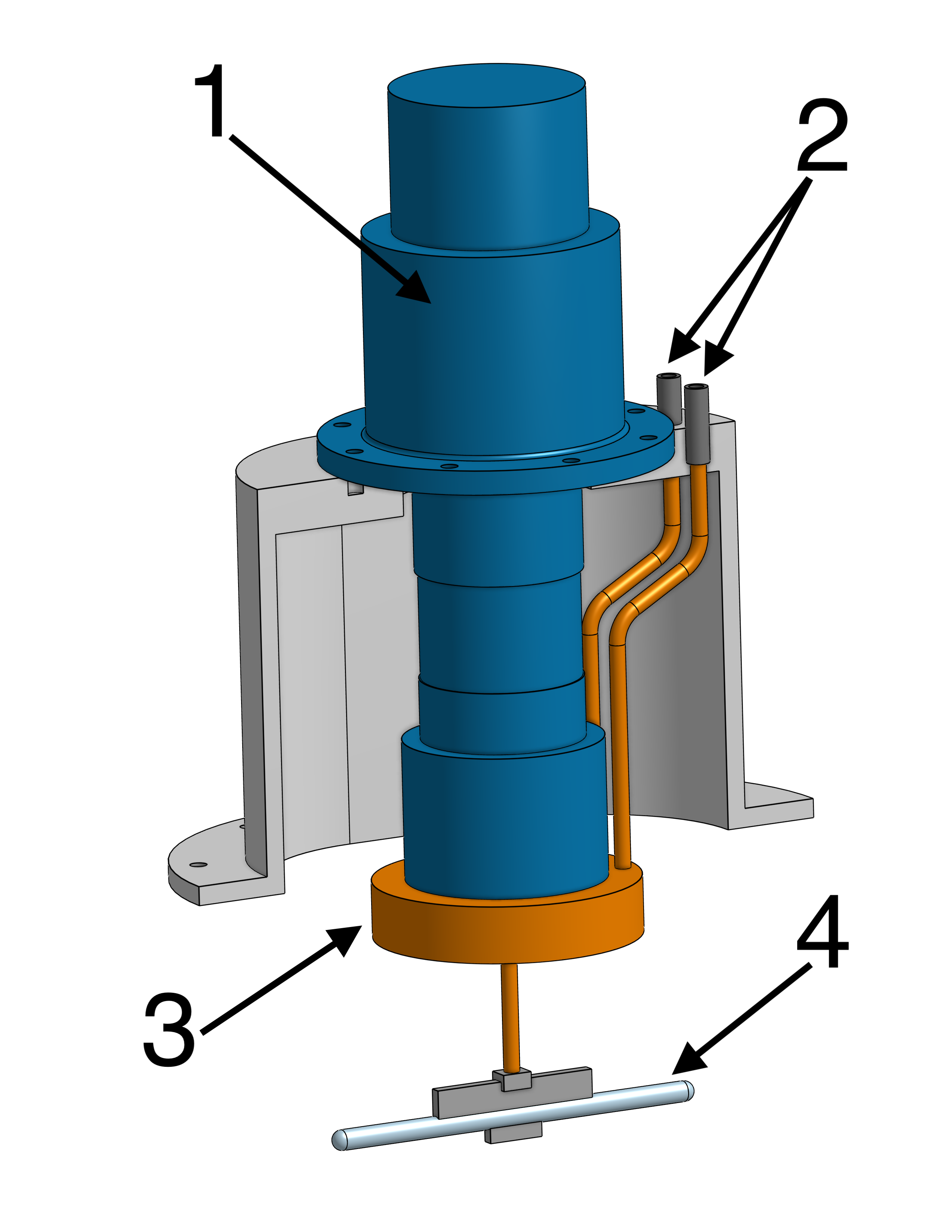
(b)

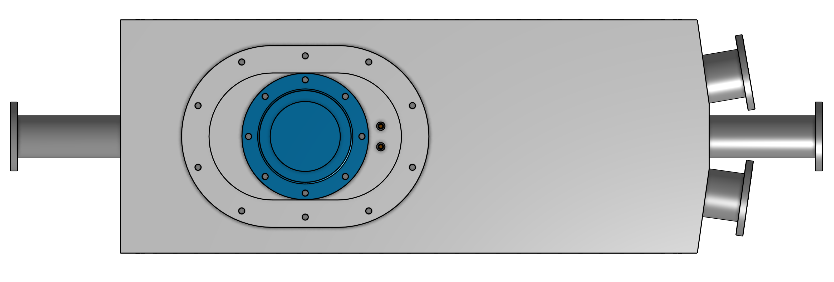
(c)

Figure 10: Conceptual design of the TPEX target chamber: (a) shows the full chamber view with the lepton beam entering from the left; (b) is a sectional drawing of the cryocooler system (1 – CH110-LT cryocooler, 2 – hydrogen supply and exhaust lines, 3 – condenser with a cooling loop, 4 – target cell), and (c) is the top view of the target chamber.

The dimensions of the scattering chamber windows shown in Fig. 10a are determined from the solid angle subtended by the calorimeters. The two side exit windows cover the polar angles for the PbWO₄ crystal calorimeters in the range of $$$<\theta<$$$. At the end of the 3 m long beampipes leading to the luminosity monitors are two tiny exit windows cover a range of $$$<\theta<$$$. The vertical dimensions of the two side exit windows cover an azimuthal angle of $\phi=$$\pm$$$.

A schematic drawing of the 20 cm long target cell is shown in Fig. 11. At the time of this proposal, it had not yet been decided if the target cell diameter should be 10 mm or 20 mm. This will in part depend on the lepton beam properties. The general aim is to minimize the target cell diameter to restrict the amount of hydrogen present in the target system, while minimizing heat load in the cell walls by the beam halo. The cell walls are made of 0.25 mm thick, drawn aluminum tubes, similar to those used for cigar tube travel cases. It is expected that the entire target system contains not more than 60 gas liters (or 75 ml LH₂) of hydrogen gas.

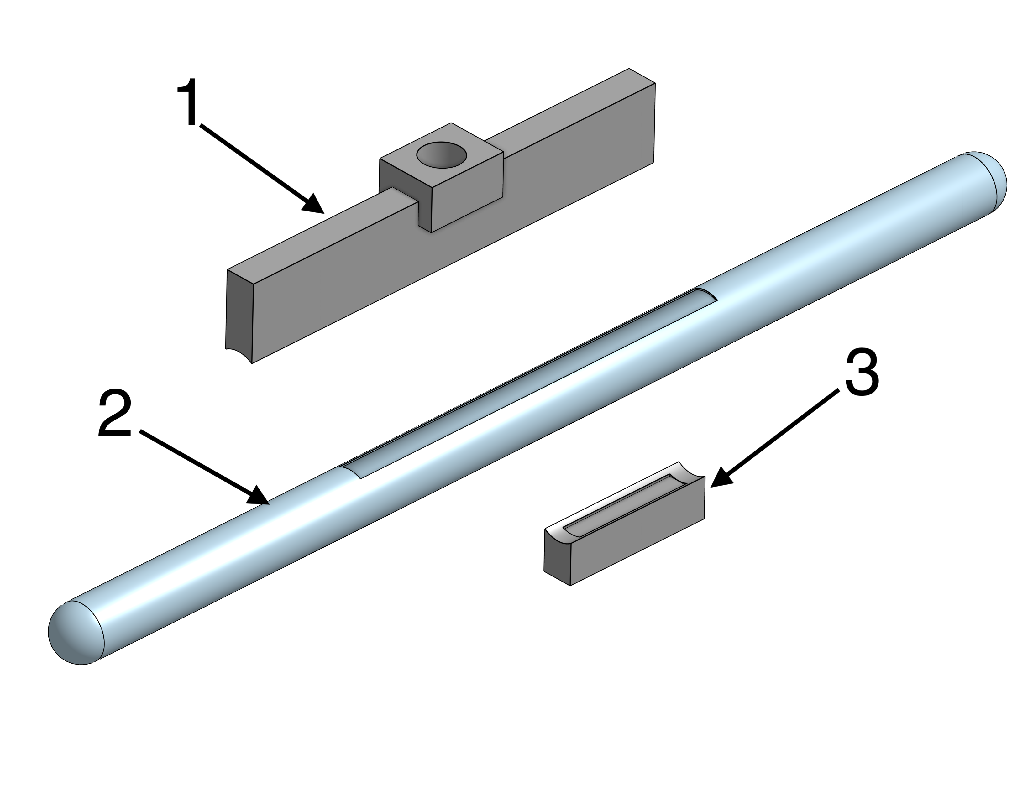
Figure 11: Design overview of the 20 cm long target cell: 1 – top block with liquid hydrogen level sensor, 2 – target cell, 3 – bottom block with temperature sensor and heater.

The maximum beam heat load for the 3 GeV electron/positron beam impinging on the 20 cm long cell at 60 nA is $H=60\,{\rm nA}\cdot 0.070\,{\rm g/cm}^{3}\cdot 20\,{\rm cm}\cdot 30\,{\rm MeV/(g/cm}^{2}{\rm)}=2.5\,{\rm W}$. The thermal, or radiation heat load on the 20 cm long and 20 mm diameter target cell is about $730\,{\rm mW}/(n+1)$, where $n$ is the number of superinsulation layers wrapped loosely around the cell. So, for the expected 10 layers of superinsulation, the thermal heat load will be approximately 70 mW, which is much smaller than the beam heat load. We expect some bubble formation in the liquid H₂ due to the heat load from the lepton beams. The long, rectangular slot in the target cell, shown in Fig. 11, allows the bubbles to escape into the top aluminum block. This helps to minimize density fluctuations and target thickness variations. The entrance and exit cups of the target cell will be thinned by chemical etching to reduce the amount of material in the beam, and thus the background caused by $e^{\pm}$ scattering off the target cell.

Liquid hydrogen will be filled through a single fill tube that serves as the return tube for the boiled off hydrogen. The fill/return tube connects the condenser, which is bolted to a cryo-cooler, with the top aluminum block also shown in Fig. 11. This aluminum block also houses two liquid hydrogen level sensors (with one serving as a backup). Each sensor is a $100\,\Omega$ Allen Bradley carbon resistor driven at 20 mA. One Lakeshore Cernox${}^{\text{\textregistered}}$ thin film resistance cryogenic temperature sensor and one ($50\,\Omega$, 50 W) cartridge heater are inside the bottom copper block. The temperature sensor, the level sensors, and the heater are all monitored and controlled by a slow control system similar to that used in the MUSE experiment [33].

The cryo-cooler/condenser combination will closely follow the successful MUSE design [33]. We will therefore use the CH110-LT single-stage cryo-cooler from Sumitomo Heavy Industries Ltd [34] for refrigeration. This cryo-cooler, in combination with the Sumitomo F-70 compressor [35], was chosen for MUSE [36] over Cryomech partly because Sumitomo has a service center in Darmstadt, Germany, while Cryomech does not have a service center in Europe. As shown in Fig. 43, the cryo-cooler has a cooling power of $25$ W at $20$ K, which is more than sufficient to cool down and fill the 70 ml LH₂ target cell in approximately 2 hours [33].

Geant4 Monte Carlo simulations will be performed for this conceptual design to verify that the experimental requirements can be met. These simulations should tell us whether the basic cell design is acceptable, or whether modifications to the scattering chamber exit windows are needed to reduce background.

4.1 Towards a functional LH₂ Target for TPEX

The Michigan group plans to work closely with the MIT-Bates engineers and an external company, Creare, Inc., to design and fabricate the system. The U-M group will start with the current conceptual design, and improvements informed by Geant4 simulations as well as the many lessons learned from building the cryogenic targets for the MUSE and SeaQuest experiments, to complete the engineering design. This will be done in close collaboration with the MIT-Bates engineers, and the external company, Creare, who has performed the engineering design and the construction of the MUSE target system. It is anticipated that this process will take about 6 months to allow sufficient time to include periodic reviews by the DESY for compliance and safety issues.

Safety precautions and the lack of a fully developed slow control system at Creare will not allow a full-blown cool-down test with LH₂ to be performed before shipment to DESY. Instead a cool-down test with neon, which has a similar boiling point as hydrogen but is not explosive, has to be performed. Once general cool-down performance and target operation in vacuum, near 20 K, has been demonstrated, the target system will be shipped to DESY where the neon test will be repeated in a staging area to ensure that all components are still functioning properly. A cool-down test with about 5 cm³ of hydrogen, an amount small enough to be safe even if it exploded in the cryostat vessel, will then be performed to start testing the slow control system and the safety procedures. Finally, a complete integration test in the Hall 2 testbeam area to fully test all components, including slow controls and safety procedures will be performed before starting the production run in the 2022.

5 Lead Tungstate Calorimeters

For the proposed experiment we are leveraging the R&D experience [37, 38] from the CMS experiment and subsequent applications by the Bonn and Mainz groups at CEBAF [39] and for PANDA [40]. We would start with ten $5\times 5$ arrays of lead tungstate (PbWO₄) crystals for a total of 250 crystals, some of which may be available from Mainz. Other configurations are possible and will be investigated with more detailed Monte Carlo simulations.

Some properties for lead tungstate are provided in appendix K. We plan to use crystals $2\times 2\times 20$ cm³. The density is 8.3 g$\cdot$cm^-3 so each crystal weighs around 664 g, or 16.6 kg for a $5\times 5$ array of crystals. Lead tungstate has a radiation length $X_{0}=0.8904$ cm, so these crystals are approximately 22.5 $X_{0}$ for good longitudinal electromagnetic shower confinement. The Molière radius is 1.959 cm, so using just the central $3\times 3$ array of crystals for acceptance, the outer ring of crystals contains the transverse shower adequately. The nuclear interaction length for lead tungstate is $\lambda_{I}=20.28$ cm, so the crystals are roughly $0.986\ \lambda_{I}$. Again, other configurations are possible and further studies and simulations are in progress. The energy resolution obtained with lead tungstate for the lepton energy range of interest is approximately 2%. The Mainz Panda readout design uses Avalanche Photo-Diodes (APD). We are also considering SiPM and PMT readout schemes.

Lead tungstate resolution varies with temperature. To achieve the best energy resolution, the crystal arrays should be maintained at a constant temperature. The best energy resolution has been obtained at $-25\degree$ C. This requires refrigeration and complicates what would otherwise be very simple and compact calorimeter modules. Results from the test runs at the DESY test beam facility on prototype lead tungstate calorimeters will be used to determine whether or not such cooling is required or if adequate resolution can be obtained with more modest cooling to have a stable temperature.

An alternative to lead tungstate is being investigated by T. Horn at Catholic University of America. She is developing high-density, ceramic glass crystals. These would be approximately 15% less dense than lead tungstate, so a larger crystal might be required. But the ceramic glass is much easier to produce and would be 5–10 times cheaper. In addition, the ceramic glass is not as sensitive to temperature, which would simplify the design. We will be testing both lead tungstate and ceramic glass in the future.

Clearly, the lead tungstate crystals will be a crucial part of the TPEX experiment. It will therefore be very important to test and maintain the quality of the crystals whether they are produced by the firm Crytur in the Czech Republic or obtained from existing supplies in Europe or America. The collaboration has colleagues from Charles University in Prague, Czech Republic who have volunteered to take responsibility for testing the crystals, verifying the quality and maintaining a database for tracking the crystals from delivery to the final calorimeter modules.

6 GEM Detectors

It is proposed to stack two Gas Electron Multiplier (GEM) detector layers with two-dimensional readout in front of each calorimeter. Thin absorbers will be placed between the target and the GEMs to stop low-energy Møller or Bhabha leptons. The GEMs provide spatial information of the traversing charged particle at the 100 micrometer precision level. The hits on two GEM elements are used to form a track segment providing directional information between the impact point on the calorimeter and the event origin in the target. This serves to suppress charged-particle backgrounds from regions other than the target. Also, the GEMs are insensitive to neutral particles, hence they provide a veto against photons and neutrons. Using the calorimeter hit as a third tracking point will allow a measure of the efficiency of each.

An active area of slightly more than 20x20 cm² is required to fully cover the area of the calorimeter entrance. A total of 20 elements is required to instrument ten calorimeter arms. The standard readout strip pitch of 0.4 mm results in 500 channels per axis, or 1,000 channels per GEM element. The full experiment would have 20,000 channels. Since the occupancy will be at the few percent level at most, zero suppression will reduce the amount of recorded data substantially.

The Hampton group has developed GEM detectors for OLYMPUS, MUSE and DarkLight. Recently, the group has established the novel scheme (NS2) of assembling GEM detectors without gluing, while stretching GEM foils mechanically within a double frame structure, for the first time for nuclear physics applications. The scheme makes the assembly fast and low risk, such that even a larger number of GEM elements can be produced fairly easily.

7 Luminosity and Beam Alignment Monitor

The relative luminosity between the electron and positron running modes is the crucial normalization for the proposed measurement. The luminosity could be monitored by a pair of small-angle detectors positioned downstream on either side of the beamline. This approach was also used in the OLYMPUS experiment [41], and based on the lessons learned from that experiment, could be improved substantially. Given the running conditions of the proposed measurement, we favor a pair of quartz Cherenkov counters positioned $8\degree$ from the beamline to monitor the rates of Møller and Bhabha scattering from atomic electrons in the target.

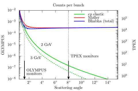
Figure 12: Whereas the forward monitors in OLYMPUS had an event per bunch rate well below 1, the TPEX monitors will see $10^{4}$ Møller or Bhabha events per bunch crossing.

In OLYMPUS, the most accurate determination of the relative luminosity was obtained from the rates of multi-interaction events—in which a Møller or Bhabha event occurred in the same bunch as a forward elastic $e^{\pm}p$ event [42]. This method had an overall uncertainty of 0.36% and looked promising for future measurements. Unfortunately it is not feasible for the proposed measurement because of the higher rate per bunch crossing, as seen in Fig. 12. The multi-interaction event method requires that the event per bunch rate to be much less than unity. However, the monitors for the proposed measurement will see approximately $10^{4}$ Møller or Bhabha events per bunch crossing.

Instead, the proposed monitor can work by integrating the signal from all particles produced during each bunch. A monitor placed at $8\degree$ has a number of advantages relative to the $1.3\degree$ placement of the OLYMPUS luminosity monitors. First, at $8\degree$, the Møller and Bhabha cross sections are only a few percent different, whereas for the OLYMPUS monitors, which covered the symmetric angle ($90\degree$ in the center-of-mass frame), the two cross sections differed by over 50%, with significant angular dependence. Second, the Møller/Bhabha rate completely dwarfs the $e^{\pm}p$ elastic scattering rate, meaning that it is really only sensitive to QED processes. No form factors or any other hadronic corrections are needed to calculate the Møller and Bhabha cross sections. Third, the sensitivity to alignment scales as $1/\sin\theta$, meaning the monitor will be much more robust to small misalignments, which were a significant problem for the OLYMPUS luminosity monitor.

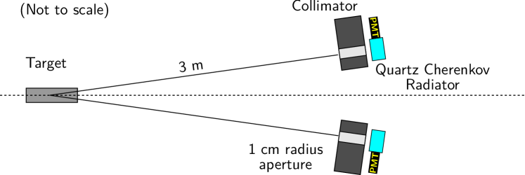
Figure 13: Schematic for the proposed luminosity monitor, consisting of two quartz Cherenkov detectors with an acceptance defined by 1 cm radius apertures in high-Z collimators

To test the feasibility of the proposed luminosity monitor, we have developed a preliminary design, and run a Monte Carlo simulation to test the sensitivity to misalignments and beam position shifts, which were the dominant systematic errors for the OLYMPUS luminosity determination [42]. A schematic of the design is shown in Fig. 13. The monitor consists of two quartz Cherenkov detectors, which act as independent monitors. Cherenkov detectors were chosen because they are widely used for monitoring in high-rate applications, such as in parity-violating electron scattering [43, 44]. The two detectors operate independently and can cross-check each other, helping to reduce systematic errors from beam alignment. In this design, the monitors are placed 3 m away from the center of the target, along the $8\degree$ scattering angle. The acceptance is defined by a collimator with a circular aperture with a radius of 1 cm.

(a)

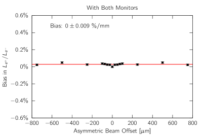
(b)

Figure 14: The potential bias from a charge-asymmetric beam misalignment is a mere 0.2%/mm in a single monitor (a), and this is completely eliminated by using a pair of monitors (b).

Fig. 14 shows the effect on the luminosity determination from beam misalignment. The most pernicious misalignment would be one that is asymmetric between electron and positron modes, and so this was the focus of this study. When using a single monitor, an asymmetric misalignment would cause a mere $0.21\pm 0.1$ %/mm bias in the determination of the relative luminosity. When using the combination of both a left and right monitor, this bias is completely eliminated to the uncertainty of this simulation. For comparison, the OLYMPUS luminosity monitor was sensitive to asymmetric misalignments at the level of 5.7 %/mm, and it was estimated that the beam position monitors could control the asymmetric misalignment to within 20 $\mu$m [42]. Such control will probably not be possible in the proposed measurement due to the much smaller beam current. However the simulation demonstrates that such control is not needed. This is largely due to the flatness of the Møller and Bhabha cross sections at $8\degree$ (see Fig. 12). One downside of this robustness is that the proposed monitors are not very sensitive as beam alignment monitors.

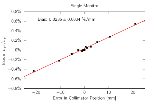
Figure 15: Errors in the positioning of the collimator aperture also have a minimal impact on the relative luminosity determination.

Fig. 15 shows the simulation results for the effect on the luminosity determination if one of the collimator apertures were to be positioned in a different place than expected. The maximum effect occurs when the collimator is shifted to a larger or smaller scattering angle, and so this was the focus of the study. For a single monitor, the effect is a mere 0.02 %/mm. In practice, both monitors can have positioning errors, and these effects could end up adding or partially canceling. Regardless, because of the positioning at $8^{\circ}$, the bias is minimal. For comparison, the effect on OLYMPUS was approximately 0.13 %/mm, with a survey accuracy of approximately 0.5 mm. Based on the experience gained from OLYMPUS, we can make improvements in the collimator positioning. One obvious improvement is to include integral survey marks on the collimator itself, since the aperture defines the monitor acceptance.

The simulation shows that two of the major systematic limitations of the OLYMPUS luminosity monitor will be minimal for the proposed design. The third major systematic, stemming from the residual magnetic field along the beamline, will be irrelevant. The proposed design does have other systematic limitations. The biggest concern will be the amplitude stability of the photomultiplier. With about $10^{4}$ particles passing through the aperture every bunch crossing, there is no way to calibrate the light yield from the data itself. To guard against gain drifts, an external calibration source will be vital. A pulsed light source, e.g. a UV laser, coupled to a fiber-optic distribution system can be used to monitor the gain of both photomultipliers throughout the experiment, while an independent photodiode can be used to cross check that the laser intensity itself does not drift. Several of us have experience with laser calibration systems used in previous experiments [45, 46]. Sub-percent level accuracy should be achievable, though this will almost certainly be the limiting systematic effect.

8 Beamdump / Faraday Cup

A new extracted beam facility from DESY II will need a beamdump. M. Schmitz (DESY) and C. Tschalar (MIT) have looked into the requirements and proposed very similar configurations with an aluminum core and a copper shell. M. Schmitz’s design was an aluminum cylinder 10 cm in diameter and 50 cm long embedded in a copper shell 22 cm in diameter and 65 cm long and had water cooling. C. Tschalar’s design was larger with 20 cm diameter and 50 cm long aluminum in a 32 cm diameter and 75 cm long copper shell but was air cooled. Both recommended that the beamdump be surrounded by neutron absorbing material like cement blocks or borated polyethylene.

Assuming a maximum current of 100 nA and a beam energy of 7 GeV the maximum power to be handled is 700 W. To contain the showering you want order of 5 Moliére radii laterally and order of 25 radiation lengths longitudinally. To be conservative we have selected C. Tschalar’s numbers as a starting point Fig. 16.

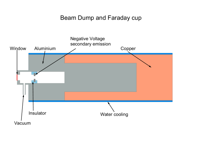
Figure 16: Schematic of a possible beamdump / Faraday cup for TPEX

To augment the luminosity measurement proposed above we thought it might be useful to modify the beamdump to function as a Faraday cup as well to integrate the charge that passes through the target. Then, assuming the length of the target cell and density of liquid hydrogen are known we can get a quick measure of the luminosity. As shown in the figure an insulated ring held at negative voltage of a few hundred volts is needed to suppress secondary emission from back scattering out of the Faraday cup. The beamdump / Faraday cup is under vacuum but this need only be roughing vacuum pressure.

9 Electronics and Readout System

The requirements for data acquisition are comparatively modest. Less than 300 channels have to be read out, including the luminosity monitor. With a readout at a low and fixed frequency, no busy logic is required.

9.1 Trigger

The beam has a very low and fixed bunch frequency of $12.5\text{\,}\mathrm{Hz}$, allowing us to trigger on the bunch clock instead of a trigger detector. The only complication is that for proper gate alignment, the beam bunch signal has to be shifted by up to 80 ms, with stability on the 10 ns level. This can be achieved with an FPGA, which can also generate the required gates. A V2495 module from CAEN is available in the collaboration and would be adequate.

9.2 Front end electronics

For the calorimeter and luminosity monitors, all proposed readout devices require the acquisition of a time-integrated current pulse with a QDC. However, they differ in the required front end electronics:

• PMTs require only a base for the high-voltage distribution. Active bases can minimize power losses and improve stability. Such bases are available commercially, or can be manufactured by the collaboration. Circuit designs are readily available and can be adapted to fit the required form factor. No further signal conditioning (except attenuation in the case of the luminosity monitors) is required for interfacing with standard QDCs.

• APDs and SiPMs require driver and preamplifier circuits. In the case of APDs, we would copy the tested design for the PANDA detector [47] from Mainz. For SiPMs, the MUSE collaboration produced an amplifier design which could be adapted [48].

9.3 Baseline DAQ hardware and software

In addition to the V2495 for trigger generation, the baseline configuration for 250+2 detectors would require eight 32-channel QDC modules like CAEN’s V792 or Mesytec’s MQDC-32. This can be housed in a single VME crate and read out via a single board computer (SBC) as the VME controller.

The data rates are low, with about $6\text{\,}\mathrm{k}\mathrm{B}\mathrm{/}\mathrm{s}$ for the readout of 252 channels at $12.5\text{\,}\mathrm{Hz}$. This makes it possible to store all experiment data to a single server outside of the experimental area via standard network file systems. This rate requires less than 4 GB per week.

The SBU group already developed the DAQ software for the test beams, which will be basis for the DAQ solution of the actual experiment.

For the GEMs, multiple readout solutions are possible:

• APV based readout, based on the MPD-4 readout boards already used for SBS@JLAB and MUSE [36]. While APVs are out of production, these collaborations have a significant number of APV readout cards and MPDs available, and experience in operating these components.

• SAMPA based readout. This is currently in development at JLab for TDIS and other projects. Compared to GEMs, the signal quality is better and the wave form can be sampled as well. There has been a lot of progress on the testing of the chips, which will be in production for the foreseeable future. However, a switch would require the procurement of new hardware.

• VMM based readout. The VMM chip is considered to be the successor to the APV chip in the Scalable Readout System (SRS). This new development is cost-effective and scalable, and has been adopted and recommended by RD-51 in the framework of the SRS readout scheme. The Mainz MAGIX collaboration recently decided to start using VMM for their GEM readout at MESA. The VMM offers readout with time and pulse shape digitization directly on the front-end card. Two VMM chips are housed on one front-end card to process 128 readout channels.

The data rate from the GEMs is considerably higher, but still manageable, particularly with zero suppression. With 1,000 channels per detector and 20 detectors, the estimated rate is between $500\text{\,}\mathrm{k}\mathrm{B}\mathrm{/}\mathrm{s}$ (1 sample per event and channel) to $\mathrm{5}$MB/s (10 samples per event and channel), resulting in about 1.5 TB per week of beam time. With zero suppression this could be reduced to a level of 300 GB per week.

9.4 Possible improvements

We are evaluating multiple improvements over this baseline design:

• Higher trigger rate: Instead of triggering just on the beam clock, the FPGA can generate additional gates before and after each trigger, spaced so that all conversion and data transmission can happen before the real gate opens. This triples the trigger and thus data rate—easily handled by the proposed system—but would allow for baseline and background monitoring.

• Instead of QDCs, which only give information about the integrated charge, the signal wave forms could be digitized with high speed ADCs. This would allow even better baseline control, but would increase the bandwidth considerably. For example, sampling the signals for $1\text{\,}\mathrm{\SIUnitSymbolMicro}\mathrm{s}$ with $250\text{\,}\mathrm{MHz}$ at 14 bit would result in about 6 kB/s per channel, less than $1.6\text{\,}\mathrm{M}\mathrm{B}\mathrm{/}\mathrm{s}$ in total. These data rates are still readily managed by the system outlined above, and about 1 TB of storage per week. Commercial solutions for these digitizers exist, but are about factor four more costly than QDCs. Cost-effective alternatives are the 12-ch WaveBoard 2.0 designed by INFN Roma/Genova or commercial boards using the DRS4 chip [49], like CAEN’s V1742. The DRS4 chip realizes an analog buffer to allow for the cost effective and high-speed (multi-GSamples/s) sampling of events. The trade-off is considerable dead-time for the conversion; however this is completely hidden in the proposed experiment by the comparably low trigger rate. The digitization of the waveform would provide additional insights into the detected particle and it’s timing, allowing us to improve background rejection.

The decision on these improvements will be based on our experience with these options in test beams planned for the near future.

10 Upgrades / Improvements to the Proposed Experiment

While the configuration proposed so far is possible and would allow the two-photon exchange contribution to be investigated in a region where the observed form factor discrepancy is clear; a number of upgrades are possible.

1. The current configuration assumes that 250 lead tungstate crystals can be obtained. Clearly if less or more crystals are possible the configuration would change. Adding more crystals to the back angle calorimeters would increase the acceptance in a region of low count rate. With an additional $5\times 5$ array above and below the current modules the solid angle would be increased from $3.6$ msr to $15.6$ msr an increase of 4.3.

2. If the showering in the $5\times 5$ arrays of PbWO₄ is well understood; it may be possible to accept a larger area of the calorimeter, say an effective area of 6.4 msr rather than the 3.6 msr using just the central $3\times 3$ array. This would increase the acceptance by $1.78$. Placing a tracking detector, e.g. GEM, immediately before the calorimeter would help to define the acceptance. This needs to be investigated with test beam studies with a $5\times 5$ calorimeter.

3. Move the back angle calorimeters closer to the target. Going to a radius of 0.5 m would increase the count rate by a factor of four, though increasing the angular range subtended and thus reduce the $Q^{2}$ resolution. Addition of GEM tracking may help this but needs further Monte Carlo simulation and study.

These options could increase the count rate significantly, making even higher beam energies accessible. Table 4 shows the kinematic reach and differential cross section for just the back angle, $110\degree$, for various lepton beam energies. A measurement at lepton beam energy of 4 GeV would extend the two-photon exchange measurements to 6.39 (GeV/$c$)², and only requires an improvement by a factor of five to be comparable to the proposed measurement rate at 3 GeV.

$E_{beam}$	$\theta$	$Q^{2}$	$\epsilon$	$d\sigma/d\Omega$
GeV		(GeV/c)2		fb
2.0	$110\degree$	2.78	0.120	$1.22\times 10^{4}$
3.0	$110\degree$	4.57	0.096	$1.20\times 10^{3}$
4.0	$110\degree$	6.39	0.080	$2.23\times 10^{2}$
5.0	$110\degree$	8.23	0.068	$5.92\times 10^{1}$
6.0	$110\degree$	10.1	0.060	$2.00\times 10^{1}$

Table 4: Kinematics and cross section for measurements at $110\degree$ for lepton beam energies possible with DESY-II

11 Background Considerations

11.1 Protons from $e^{\pm}p$ elastic scattering

As proposed, the experiment does not measure the scattered lepton and proton in coincidence. While this would have some benefits it would also require detectors at far forward angles where the event rates from elastic lepton scattering, Møller and Bhabha scattering, and pion production would be problematic. Nevertheless, protons from elastic lepton-proton scattering will strike the proposed detectors and will be a source of background for the measurement.

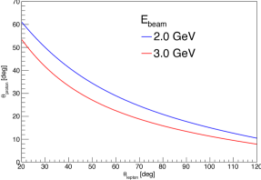
(a)

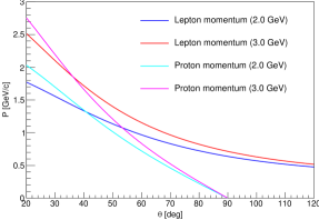
(b)

Figure 17: Kinematics for $ep$ elastic scattering. (a) Proton scattering angle as a function of the lepton scattering angle. (b) Lepton and proton momenta as a function of their respective scatting angles.

Fig. 17a shows the relation between the proton polar scattering angle and the lepton scattering angle. Fig. 17b shows the momentum for the lepton and proton as a function of their scattering angle. The proton momentum is greater than that of the lepton at forward angles but drops more rapidly as its scattering angle increases. Protons will also be detected in the calorimeters and will have to be identified and corrected for on an event by event basis. The calorimeter modules at over 22 $X_{0}$ will adequately contain the electromagnetic showers and detect most of the lepton energy, but the proton will not deposit its full energy as the calorimeter is only around one nuclear interaction length in depth. Monte Carlo studies (presented below) indicate that the proton will deposit at most 300 to 400 MeV in the calorimeters at $30\degree$ and $50\degree$ and significantly less at larger angles, particularly if an absorber shield is placed in front of the calorimeters. This will allow the lepton signal to be clearly resolved from the proton signal.

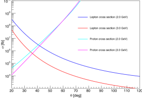
(a)

(b)

Figure 18: Kinematics for $ep$ elastic scattering. (a) Cross sections for lepton and proton as a function of their polar angle. (b) Beta for the proton as a function of its polar angle.

At $30\degree$ the proton rate will be an occasional nuisance as it is significantly less than the lepton rate as shown in Fig. 18a. However, at $50\degree$ the proton rate will be 10–100 times that for the lepton. This is still not a problem, as the rate is manageable (approximately once every three beam spills) plus the deposited proton energy will be more than 700 MeV lower than the lepton’s. But, at $70\degree$ the rate for protons is $10^{4}-10^{5}$ greater than that for leptons resulting in multiple protons from every beam spill. However, as discussed in the Monte Carlo section, with a suitable absorber the protons can be stopped before the calorimeter without significantly affecting the lepton signal. It may also be possible to eliminate this if the calorimeter timing and readout is sufficiently fast. The $\beta$ value for the proton is shown in Fig. 18b and is around 0.5 at $70\degree$. That means the protons will arrive around 3 ns after the lepton possibly allowing a timing window to exclude them. At $90\degree$ the proton rate is even higher but the energy is much lower and can be handled by an absorber and/or timing.

11.2 Møller and Bhabha scattering

The cross sections for Møller and Bhabha scattering into the detector angles being considered in this proposal are given in Table 5. For an average lepton current of 40 nA incident on a 20 cm liquid hydrogen target the luminosity is $2.11\times 10^{-4}$ fb${}^{-1}\cdot$ s^-1. If we consider the face of the entire $5\times 5$ array of each calorimeter module this corresponds to 10 msr so the luminosity factor becomes $2.11\times 10^{-6}$. Multiplying this factor through the cross sections in Table 5 yields rates ranging from around 4 to $2\times 10^{9}$ events per second.

$\theta$	Møller	Bhabha $e^{+}$	Bhabha $e^{-}$
	fb	fb	fb
2.0 GeV
$30\degree$	$1.223\times 10^{14}$	$2.863\times 10^{8}$	$1.219\times 10^{14}$
$50\degree$	$2.991\times 10^{14}$	$3.866\times 10^{7}$	$2.989\times 10^{14}$
$70\degree$	$1.986\times 10^{15}$	$9.089\times 10^{6}$	$1.985\times 10^{15}$
$90\degree$	diverges	0	diverges
$110\degree$	0	0	0
3.0 GeV
$30\degree$	$1.223\times 10^{14}$	$1.274\times 10^{8}$	$1.220\times 10^{14}$
$50\degree$	$2.991\times 10^{14}$	$1.719\times 10^{7}$	$2.989\times 10^{14}$
$70\degree$	$1.985\times 10^{15}$	$4.041\times 10^{6}$	$1.985\times 10^{15}$
$90\degree$	diverges	0	diverges
$110\degree$	0	0	0

Table 5: Cross section for Møller and Bhabha scattering as a function of the polar scattering angle.

The energies of these Møller and Bhabha scattered leptons are low, less than 4 MeV at $30\degree$ and even lower at the larger angles. For the most part they are still relativistic so a timing cut is not possible except at $90\degree$ and possibly at $70\degree$ if the calorimeter electronics are fast. To sweep these leptons away would require a magnetic field around 400 G. However, Monte Carlo studies show that a simple 10 mm aluminum absorber before the calorimeter modules will stop these particles from producing any signal in the calorimeter without degrading the response to the higher energy leptons of interest. Since a 10 mm aluminum plate over the front face of the calorimeter array would work well as part of the cooling system; the high rate of Møller and Bhabha scattered leptons is not a problem.

11.3 Pion Production

Another source of background comes from pion production. There are four reactions to consider:

$$e^{-}+p \rightarrow e^{-}+p+\pi^{0}$$ (2)

$$e^{-}+p \rightarrow e^{-}+n+\pi^{+}$$ (3)

$$e^{+}+p \rightarrow e^{+}+p+\pi^{0}$$ (4)

$$e^{+}+p \rightarrow e^{+}+n+\pi^{+}$$ (5)

A Monte Carlo pion event generator was used to simulate these four reactions at 2 and 3 GeV. The calorimeter modules in the proposed configuration will be struck by the leptons (electrons or positrons), baryons (protons or neutrons), and pions ($\pi^{0}$ or $\pi^{+}$) from the various pion production reactions. In the case of $\pi^{0}$ production the most likely decay to two photons must also be considered.

The event rate per day and the momentum distribution of the leptons, baryons, and pions incident on the $5\times 5$ calorimeter array at $30\degree$ for the reactions $e^{-}+p\rightarrow e^{-}+p+\pi^{0}$ and $\rightarrow e^{-}+n+\pi^{+}$ for an incident electron beam energy of 2 and 3 GeV are given in Fig. 19. (N.B. No accounting for $\pi^{0}$ decay or the energy actually deposited in the calorimeters has been made. A more complete Monte Carlo simulation is in progress and further plots for pion production are provided in the Appendix.)

The total event rate for electrons from pion production at 2 GeV striking the $5\times 5$ face of the calorimeter array at $30\degree$ is $2.07\times 10^{6}$ per day. This is comparable to the $7.92\times 10^{5}$ events per day expected in the central $3\times 3$ array for the elastic scattering events we wish to detect. However, the elastic events are peaked around a momentum of 1.56 GeV/c while the lepton momentum from pion production has a small peak around 1.35 GeV/c and a long tail to much lower momenta. With PbWO₄’s excellent energy resolution this difference should be easily resolved. The rates at this angle are such that we can expect one of these pion events every beam spill. This background must be detected and corrected on an event by event basis. The deposited energies of the baryons and pions are significantly lower but will also contribute to the background and will need to be handled in the analysis.

(a)

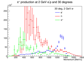
(b)

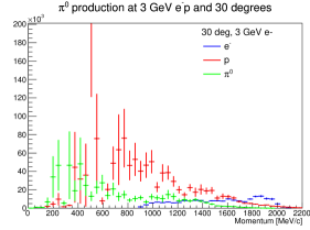
(c)

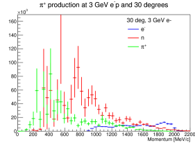
(d)

Figure 19: Number of particles directed towards the $5\times 5$ calorimeter array situated at $30\degree$ from the reactions (a) $e^{-}+p\rightarrow e^{-}+p+\pi^{0}$ and (b) $e^{-}+p\rightarrow e^{-}+p+\pi^{+}$ at 2 GeV and (c) $e^{-}+p\rightarrow e^{-}+p+\pi^{0}$ and (d) $e^{-}+p\rightarrow e^{-}+p+\pi^{+}$ at 3 GeV during one day of running at the nominal luminosity.

$\theta$	$e^{-}+p+\pi^{0}$	$e^{-}+n+\pi^{+}$	$e^{+}+p+\pi^{0}$	$e^{+}+n+\pi^{+}$
2.0 GeV
$30\degree$	$2.08\times 10^{6}$	$2.06\times 10^{6}$	$2.06\times 10^{6}$	$2.08\times 10^{6}$
$50\degree$	$2.64\times 10^{5}$	$2.54\times 10^{5}$	$2.60\times 10^{5}$	$2.56\times 10^{5}$
$70\degree$	$7.22\times 10^{4}$	$7.14\times 10^{4}$	$7.28\times 10^{4}$	$7.16\times 10^{4}$
$90\degree$	$2.86\times 10^{4}$	$2.90\times 10^{4}$	$2.84\times 10^{4}$	$2.90\times 10^{4}$
$110\degree$	$1.40\times 10^{4}$	$1.45\times 10^{4}$	$1.41\times 10^{4}$	$1.38\times 10^{4}$
3.0 GeV
$30\degree$	$4.02\times 10^{5}$	$4.08\times 10^{5}$	$4.08\times 10^{5}$	$4.06\times 10^{5}$
$50\degree$	$6.60\times 10^{4}$	$6.60\times 10^{4}$	$6.64\times 10^{4}$	$6.62\times 10^{4}$
$70\degree$	$6.58\times 10^{3}$	$6.54\times 10^{3}$	$6.64\times 10^{3}$	$6.72\times 10^{3}$
$90\degree$	$2.24\times 10^{3}$	$2.26\times 10^{3}$	$2.20\times 10^{3}$	$2.26\times 10^{3}$
$110\degree$	$9.22\times 10^{2}$	$9.10\times 10^{2}$	$9.50\times 10^{2}$	$9.32\times 10^{2}$

Table 6: Event rates per day for leptons from pion production striking the $5\times 5$ calorimeter detector arrays.

Fig. 19 shows the number of particles detected per day at the calorimeter positioned at $30\degree$ for each particle produced in pion production from $e^{-}p$ at 2 and 3 GeV. The plots for $e^{+}p$ are similar and plots for all detector angles are given in the appendix. At higher angles the lepton rates fall quickly and are broadly distributed in momentum. The rates for protons and neutrons also fall quickly plus they deposit little energy in the calorimeters. Pion rates remain fairly uniform with angle but are at a low momentum and as Monte Carlo studies indicate the deposited energy is even less. The $\pi^{0}$ decay to two photons however will be a rather uniform, low energy background. Further Monte Carlo studies are needed to verify that the background events can be cleanly resolved from the lepton signals that need to be measured.

$\theta$	$e^{-}+p+\pi^{0}$	$e^{-}+n+\pi^{+}$	$e^{+}+p+\pi^{0}$	$e^{+}+n+\pi^{+}$
2.0 GeV
$30\degree$	$6.96\times 10^{6}$	$6.04\times 10^{6}$	$5.08\times 10^{6}$	$6.64\times 10^{6}$
$50\degree$	$7.14\times 10^{6}$	$7.70\times 10^{6}$	$7.16\times 10^{6}$	$7.06\times 10^{6}$
$70\degree$	$5.14\times 10^{5}$	$9.74\times 10^{5}$	$5.30\times 10^{5}$	$8.86\times 10^{5}$
$90\degree$	$0$	$0$	$0$	$0$
$110\degree$	$0$	$0$	$0$	$0$
3.0 GeV
$30\degree$	$2.42\times 10^{6}$	$2.46\times 10^{6}$	$2.62\times 10^{6}$	$3.26\times 10^{6}$
$50\degree$	$3.76\times 10^{6}$	$3.56\times 10^{6}$	$3.38\times 10^{6}$	$3.86\times 10^{6}$
$70\degree$	$7.02\times 10^{4}$	$6.56\times 10^{4}$	$7.26\times 10^{4}$	$9.30\times 10^{4}$
$90\degree$	$0$	$0$	$0$	$0$
$110\degree$	$0$	$0$	$0$	$0$

Table 7: Event rates per day for baryons from pion production striking the $5\times 5$ calorimeter detector arrays.

$\theta$	$e^{-}+p+\pi^{0}$	$e^{-}+n+\pi^{+}$	$e^{+}+p+\pi^{0}$	$e^{+}+n+\pi^{+}$
2.0 GeV
$30\degree$	$2.78\times 10^{6}$	$2.18\times 10^{6}$	$2.02\times 10^{6}$	$2.54\times 10^{6}$
$50\degree$	$4.50\times 10^{6}$	$4.04\times 10^{6}$	$4.36\times 10^{6}$	$5.18\times 10^{6}$
$70\degree$	$3.36\times 10^{6}$	$4.44\times 10^{6}$	$4.10\times 10^{6}$	$3.94\times 10^{6}$
$90\degree$	$2.90\times 10^{6}$	$2.52\times 10^{6}$	$2.50\times 10^{6}$	$2.86\times 10^{6}$
$110\degree$	$1.68\times 10^{6}$	$1.81\times 10^{6}$	$1.21\times 10^{6}$	$1.95\times 10^{6}$
3.0 GeV
$30\degree$	$1.04\times 10^{6}$	$1.34\times 10^{6}$	$1.35\times 10^{6}$	$1.48\times 10^{6}$
$50\degree$	$2.10\times 10^{6}$	$1.96\times 10^{6}$	$1.46\times 10^{6}$	$1.60\times 10^{6}$
$70\degree$	$1.53\times 10^{5}$	$1.39\times 10^{6}$	$1.81\times 10^{6}$	$1.34\times 10^{6}$
$90\degree$	$8.16\times 10^{5}$	$7.58\times 10^{5}$	$6.10\times 10^{5}$	$6.68\times 10^{5}$
$110\degree$	$4.20\times 10^{5}$	$3.18\times 10^{5}$	$3.22\times 10^{5}$	$2.80\times 10^{5}$

Table 8: Event rates per day for pions from pion production striking the $5\times 5$ calorimeter detector arrays.

Table 6 gives the daily event rates for the leptons from pion production striking the $5\times 5$ array of each calorimeter. These rates should be compared with those in Table 1 and Table 2 that give the rates for the events of interest striking the central $3\times 3$ array. The lepton rate from pion production is generally higher than the elastic scattered events of interest. However, the lepton events of interest, arising from elastic $ep$ scattering, are peaked at significantly higher energies while the lepton energies from pion production are lower in energy and distributed over a broad range.

Table 7 and Table 8 give the corresponding daily rates for the baryons and pions striking the $5\times 5$ array of each calorimeter. While these rates by themselves are comparable to the elastic $ep$ events of interest the energy actually deposited in the calorimeter will be significantly less and should be readily distinguished from the elastic lepton signal. Of course more detailed Monte Carlo simulations are necessary and these are in progress.

12 Monte Carlo Simulations

In order to study the energy deposited in the $5\times 5$ calorimeter arrays proposed in this document a simple GEANT4 Monte Carlo [50] simulation was developed. Beams of electrons, protons, and pions ($\pi^{+}$ and $\pi^{0}$) were directed through 1 m of air at the center of a $5\times 5$ calorimeter array at normal incidence. Initial momenta of 100 MeV/c to 2500 MeV/c in 100 MeV/c steps were studied.

Four combinations of absorbers (none, 10 mm Al, 10 mm Al + 10 mm Pb, and 10 mm Al + 20 mm Pb) were placed at the front face of the calorimeter array to study the effect this would have. The 10 mm aluminum plate would naturally form part of the cooling system needed to obtain a stable energy resolution from the PbWO₄ crystals. The various thicknesses of lead were introduced to study how this could be used to reduce background from protons and pions and the effect this would have on the lepton signal.

Fig. 20 illustrates the Monte Carlo studies performed. With the simulations, details of the longitudinal and transverse energy distributions can be studied though in an actual experiment only the energy deposited in the individual crystals are available. However, these studies show that the electron shower is effectively contained longitudinally and the transverse distribution is narrow. Further studies will investigate the reconstruction of position and angle from the energy deposited in the crystals alone and also unfolding events with multiple incident particles.

(a)

(b)

(c)

Figure 20: Monte Carlo studies of electron showering in a $5\times 5$ PbWO₄ calorimeter. Incident electron momentum was 1000 MeV and a 10 mm aluminum absorber was placed before the crystals. (a) Longitudinal energy distribution. (b) Total energy detected by each crystal. (c) Transverse energy distribution in the calorimeter.

Results for various incident particles and absorbers are presented as a function of the particle momentum and absorber thicknesses in the following sections.

12.1 Electrons and Positrons

As shown in Fig. 21 a lepton incident on the central crystal of the calorimeter array deposits almost all its energy in the calorimeter. Most of that energy ($\sim 80\%$) is in the central crystal. The shower width is also quite narrow ($\sim 10$ mm). Note that the 10 mm aluminum absorber has almost no effect on the lepton shower. The lead absorber increases the transverse width of the shower significantly at low momenta and to a lesser degree at higher momenta resulting in some losses in total energy and the percentage deposited in the central crystal.

Not surprisingly positrons have a virtually identical behavior and are therefore not plotted separately here.

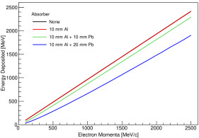
(a)

(b)

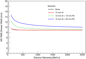
(c)

Figure 21: Electron showering in a $5\times 5$ PbWO₄ calorimeter array as a function of incident electron momentum with different absorbers. (a) Sum of energies in all 25 crystals, (b) Percentage of energy in the central crystal, and (c) RMS width of transverse shower development.

12.2 Protons

Fig. 22 shows the results for proton incident on the calorimeter array. The total energy deposited in the calorimeter is significantly less than the incident energies and for the most part is a third for momenta below 1000 MeV/c and between 300 and 400 MeV/c for higher momenta. This is consistent with the calorimeter being only one nuclear interaction length in depth so the proton has a tendency to pass straight through depositing only a fraction of its energy. Most of the energy deposited ($\sim 70\%$) is in the struck crystal. The absorbers have little effect except at low incident momenta where the proton can be completely absorbed. This may be useful in stopping the large number of lower energy protons produced at backward angles as well as low energy protons from pion production.

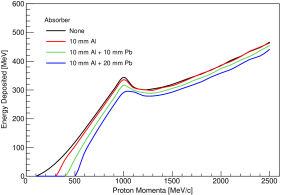
(a)

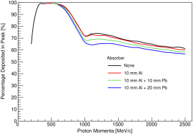
(b)

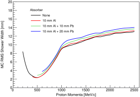
(c)

Figure 22: Proton showering in a $5\times 5$ PbWO₄ calorimeter array as a function of incident proton momentum and different absorbers. (a) Sum of energies deposited in all 25 crystals, (b) Percentage of energy in the central crystal, and (c) RMS width of transverse shower development.

12.3 Neutrons

Fig. 23 shows the results for neutrons incident on the calorimeter array. The total energy deposited in the calorimeter just 5%–15% of the incident energies. About 50% of the energy deposited is in the struck crystal. The absorbers have little effect.

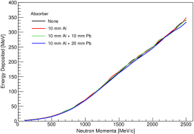
(a)

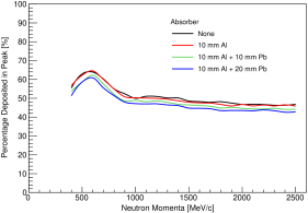
(b)

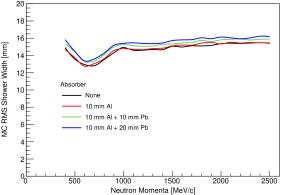
(c)

Figure 23: Neutron showering in a $5\times 5$ PbWO₄ calorimeter array as a function of incident neutron momentum and different absorbers. (a) Sum of energies deposited in all 25 crystals, (b) Percentage of energy in the central crystal, and (c) RMS width of transverse shower development.

12.4 $\pi^{+}$

Fig. 24 shows the calorimeter response to incident $\pi^{+}$ mesons. The total energy deposited in the calorimeter array varies from around 50% of the incident momenta below 500 MeV to 25% at higher momenta. The various absorber thicknesses have a small effect. 50%–60% is deposited in the central crystal and the RMS width for the transverse shower development is fairly constant around 14 mm. This reduced signal from $\pi+$ will aid in distinguishing them from the leptons of interest. Response with $\pi^{-}$ mesons is similar.

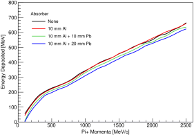
(a)

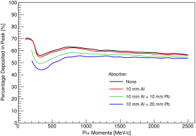
(b)

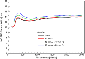
(c)

Figure 24: $\pi^{+}$ showering in a $5\times 5$ PbWO₄ calorimeter array as a function of incident pion momentum with different absorbers. (a) Sum of energies deposited in all 25 crystals, (b) Percentage of energy in the central crystal, and (c) RMS width of transverse shower development.

12.5 $\pi^{0}$

Fig. 25 shows the calorimeter response to $\pi^{0}$ mesons originating at the target 1 m away. The $\pi^{0}$s primarily decay isotropically to two photons that may or may not strike the calorimeter. For low energies the probability is small and very little energy is deposited in the calorimeter. At higher energies the two photons are boosted in the direction of the calorimeter and deposit a more significant fraction of their original energy. The energy deposited is, in any case, spread over a large area and not restricted to the central crystal as can be seen from the plots of the percentage in the central crystal and the RMS width of the shower development.

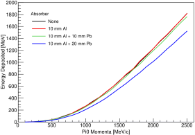
(a)

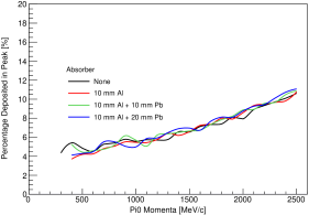
(b)

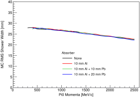
(c)

Figure 25: $\pi^{0}$ showering in a $5\times 5$ PbWO₄ calorimeter array as a function of incident pion momentum with different absorbers. (a) Sum of energies deposited in all 25 crystals, (b) Percentage of energy in the central crystal, and (c) RMS width of transverse shower development.

13 Test Beam at DESY

The Monte Carlo studies discussed in the previous section are encouraging. The proposed experiment can make a significant and direct measurement of the two-photon contribution in a region of $Q^{2}$ and $\epsilon$ where the discrepancy is clear. However, the Monte Carlo studies must be verified. It is therefore important that the performance of the calorimeter modules be studied in a test beam.

An initial prototype calorimeter was tested at the DESY test beam facility in the fall, 2019. The results are reported here in appendix A. These initial tests with a small $3\times 3$ prototype design are encouraging with good agreement with the Monte Carlo but further tests are needed.

We propose to perform these measurements at the DESY test beam facility [32] using a $5\times 5$ calorimeter array. The purpose of the test beam activity will be to measure the performance of the PbWO₄ calorimeter array and to verify the Monte Carlo simulations. We would use various energies, with and without the absorber plates, and incident at various positions and angles across the calorimeter array. Monte Carlo simulations can suggest and be used to train reconstruction algorithms but these need to be verified with actual measurements therefore the proposed test beam studies are very important.

If the ceramic glass crystals being developed by Tanja Horn (CUA) are available we would also test these in the prototype calorimeters. This clearly has links with efforts underway in Europe and the United States for future detectors for the proposed Electron-Ion Collider.

14 Conclusion

The observed discrepancy in the proton form factor ratio is a fundamental problem in nuclear physics and possibly in quantum electrodynamics. Why are the leading order QED radiative corrections insufficient to resolve the discrepancy? Are higher order corrections necessary or are more detailed models for the intermediate hadronic state needed? Or is some other process responsible?

An extracted positron and electron beam facility at DESY would provide a unique opportunity to measure the two-photon exchange contribution to elastic lepton-proton scattering over a kinematic range where the observed discrepancy is clearly evident. The above proposal outlines an initial plan for an experimental configuration that could help resolve this issue and provide insight to the radiative corrections needed to understand the proton form factors at higher momentum transfers.

Appendix A Test Beam Results

Over two weeks in September-October, 2019, a calorimeter consisting of a $3\times 3$ array of PbWO₄ crystals was studied at the DESY test beam facility [32]. Tests were made scanning the electron beam across the face of the calorimeter and with different thicknesses of absorber plates. We also compared, in parallel, a traditional, triggered readout with a streaming readout scheme. Further test beam studies were made in the fall of 2021 and spring of 2022 using a more realistic $5\times 5$ array of lead tungstate crystals. This calorimeter was also cooled and measured at 25°, 10°, -10°, and -25°C. A small number of high-density ceramic glass crystals were also tested. The analysis of the 2022 test run is ongoing.

A.1 Calorimeter Setup and Tests

The calorimeter used nine $2\times 2\times 20$ cm³ lead tungstate crystals read out using Hamamatsu R1166 PMTs attached to one end of each crystal. The crystals were wrapped with one layer of white Tyvek (0.4 mm thick) and an outer layer of opaque aluminum foil (0.09 mm thick). The crystal-PMT assemblies were placed inside a black anodized aluminum housing. See Fig. 26. Copper tubes for water cooling were installed on the outside of the aluminum box. The calorimeter assembly was mounted on an XY translation table but was electrically isolated from the table. A collimator and a set of four thin scintillators upstream of the calorimeter were using in the triggered readout.

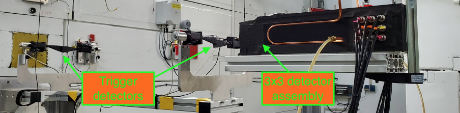
Figure 26: Photo of 3x3 lead tungstate calorimeter prototype and trigger detectors used in initial test run at DESY.

High voltage for the PMTs was provided by LeCroy 1461N modules.

Signals from the PMTs were divided by a 50 $\Omega$ splitter. One side of each splitter output was connected through a 100 ns delay cable to CAEN V792 QDC. The signals from the four thin scintillators were combined in a coincidence unit requiring a triple coincidence that was used to trigger the QDC. The other splitter output was connected to a CAEN V1725 digitizer. Since the digitizer had only 8 channels a decision was made to read out crystals 1 to 7, and use channel 0 to record the trigger signal in parallel.

The gain from each crystal and PMT was matched using a 5.2 GeV beam incident on the center of the crystal and the HV adjusted to give a common value close to the end of the QDC range.

Data were collected at beam energies of 2, 3, 4, and 5 GeV and with $2\times 2$ mm² and $8\times 8$ mm² collimators. For all conditions scans were made over the face of the calorimeter and using 0, 1, and 2 cm thick lead absorber plates before the calorimeter. Typical energy spectra for all four beam energies can be seen in Fig. 27. The left figure shows the QDC spectra (with pedestal subtraction) and the right figure the digitizer spectra for events which are in coincidence with the trigger signal.

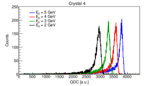
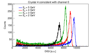
Figure 27: Deposited energy in central crystal recorded by QDC (left) and digitizer (right). The digitizer spectra also required a coincidence with a trigger signal in digitizer channel 0.

Fig. 28 shows the sum of all 25 signals with a 5 GeV beam centered on the central crystal. The root analysis tool functions “gaus” and “crystalball” were used to fit the spectra to determine peak position.

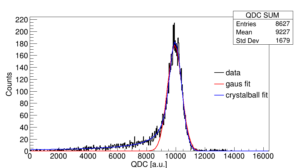
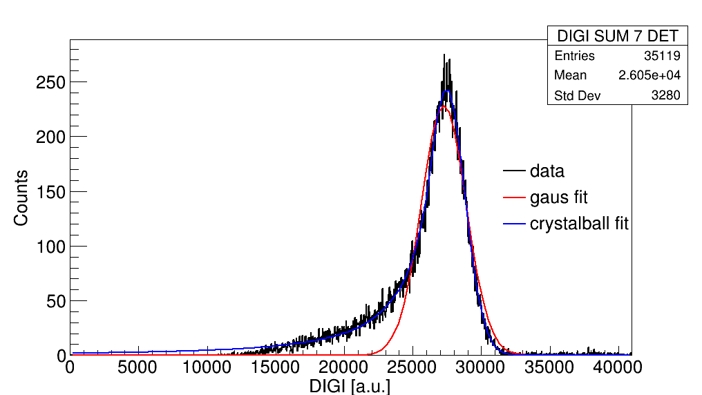
Figure 28: Sum of energies deposited in all crystals recorded by QDC (left) and digitizer. The digitizer spectrum also required a coincidence with the trigger signal in channel 0.

Linearity of the peak position with incident energy is shown in Fig. 29.

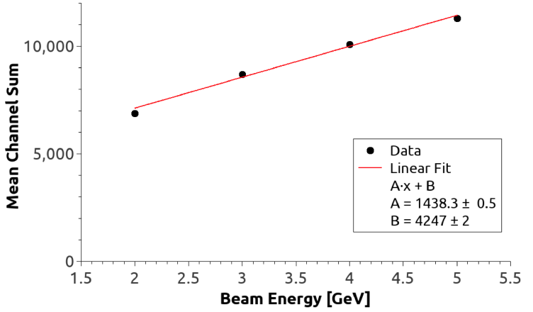
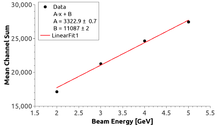
Figure 29: Energy dependence of the peak position in QDC (left) and digitizer (right).

A.2 Streaming and triggered readout

In the triggered readout scheme all channels of the QDC are read out together after receiving a trigger signal. This takes some time during which the QDC is unable to record new events (deadtime). On the other hand the streaming readout scheme using the digitizer continuously records events in all channels. Thus, the streaming system records more events in individual channels though many signals may be uncorrelated from cosmic rays, noise, or background events. To make sense of the large amount of data collected by the digitizer it is necessary to determine the relative timing of all channels. Then signals at a common time can be reasonably assumed to arise from the same event, like corresponding to showering in the calorimeter (see Fig. 30).

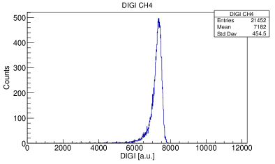
Figure 30: Deposited energy in central detector (channel 4) with coincidence signals in at least 6 neighboring crystals.

Similarly, the relative timing to the trigger signal used for the QDC (connected to channel 0 of the digitizer) can be determined and used to compare the same event collected by the QDC with that recorded by the digitizer.

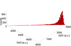
Figure 31: Left figure shows the energy deposited in the digitizer versus that for the QDC. The right figure is the 3D histogram plot of the same data.

A.3 Monte Carlo Simulation of Test Beam

A Monte Carlo simulation of the test beam was developed in Geant4 [50]. We use the FTFP_BERT physics list provided by Geant to simulate the showers and energy loss processes in the crystals. We reproduced the TB24/1 area from the available drawings and technical details provided by DESY. This included the calorimeter, absorber plates, trigger scintillators, collimator, and the origin of the beam source at the DESY II ring. This last item was found to be very important to account for the significant energy straggling observed in the measured spectra. The Geant4 visualization of the front face of the $3\times 3$ calorimeter array is shown in Fig. 32.

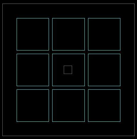
Figure 32: The Geant4 simulation view of the front face of the calorimeter.

Fig. 33 shows a comparison between the measured QDC data and the simulation for the central crystal for a 2 GeV incident beam.

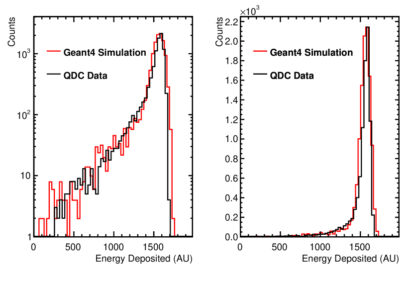
Figure 33: Comparison between Geant4 simulation and data from the QDCs using logarithmic (left) and linear (right) scales. The simulation is scaled to the height of the data.

Fig. 34 shows a similar comparison between simulation and the digitizer data. The discrepancies between simulation and data can be ascribed to an incomplete model of the experimental hall, specifically any material causing energy loss upstream of the hall. We believe with improved modeling the agreement could be better.

Figure 34: Comparison between Geant4 simulation and data from the digitizers. The simulation is scaled to the height of the data.

Appendix B Monte Carlo Simulation for $e^{-}+p\rightarrow e^{-}+p+\pi^{0}$ at 2 GeV

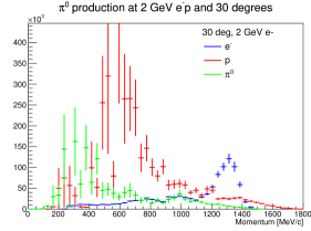
(a)

(b)

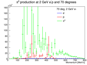
(c)

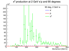
(d)

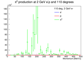
(e)

Figure 35: Number of electrons, protons, and $\pi^{0}$ directed towards the $5\times 5$ calorimeter arrays at $30\degree$, $50\degree$, $70\degree$, $90\degree$, and $110\degree$ during one day of running at the nominal luminosity for the reaction $e^{-}+p\rightarrow e^{-}+p+\pi^{0}$ at 2 GeV.

Appendix C Monte Carlo Simulation for $e^{-}+p\rightarrow e^{-}+n+\pi^{+}$ at 2 GeV

(a)

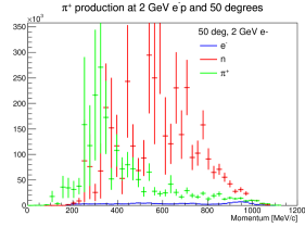
(b)

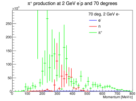
(c)

(d)

(e)

Figure 36: Number of electrons, neutrons, and $\pi^{+}$ directed towards the $5\times 5$ calorimeter arrays at $30\degree$, $50\degree$, $70\degree$, $90\degree$, and $110\degree$ during one day of running at the nominal luminosity for the reaction $e^{-}+p\rightarrow e^{-}+n+\pi^{+}$ at 2 GeV.

Appendix D Monte Carlo Simulation for $e^{+}+p\rightarrow e^{+}+p+\pi^{0}$ at 2 GeV

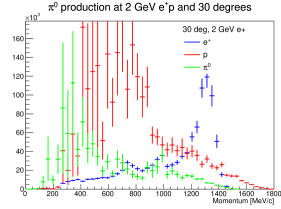
(a)

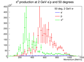
(b)

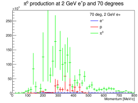
(c)

(d)

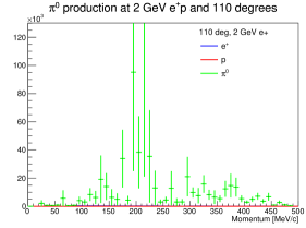
(e)

Figure 37: Number of positrons, protons, and $\pi^{0}$ directed towards the $5\times 5$ calorimeter arrays at $30\degree$, $50\degree$, $70\degree$, $90\degree$, and $110\degree$ during one day of running at the nominal luminosity for the reaction $e^{+}+p\rightarrow e^{+}+p+\pi^{0}$ at 2 GeV.

Appendix E Monte Carlo Simulation for $e^{+}+p\rightarrow e^{+}+n+\pi^{+}$ at 2 GeV

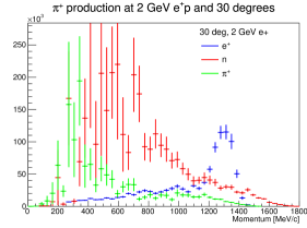
(a)

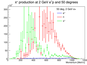
(b)

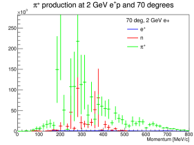
(c)

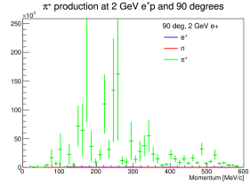
(d)

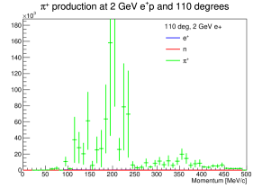
(e)

Figure 38: Number of positrons, neutrons, and $\pi^{+}$ directed towards the $5\times 5$ calorimeter arrays at $30\degree$, $50\degree$, $70\degree$, $90\degree$, and $110\degree$ during one day of running at the nominal luminosity for the reaction $e^{+}+p\rightarrow e^{+}+n+\pi^{+}$ at 2 GeV.

Appendix F Monte Carlo Simulation for $e^{-}+p\rightarrow e^{-}+p+\pi^{0}$ at 3 GeV

(a)

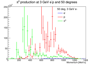
(b)

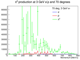
(c)

(d)

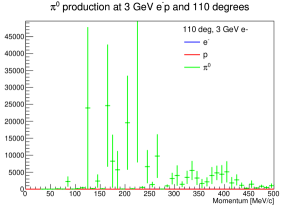
(e)

Figure 39: Number of electrons, protons, and $\pi^{0}$ directed towards the $5\times 5$ calorimeter arrays at $30\degree$, $50\degree$, $70\degree$, $90\degree$, and $110\degree$ during one day of running at the nominal luminosity for the reaction $e^{-}+p\rightarrow e^{-}+p+\pi^{0}$ at 3 GeV.

Appendix G Monte Carlo Simulation for $e^{-}+p\rightarrow e^{-}+n+\pi^{+}$ at 3 GeV

(a)

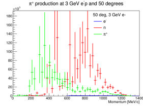
(b)

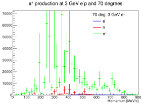
(c)

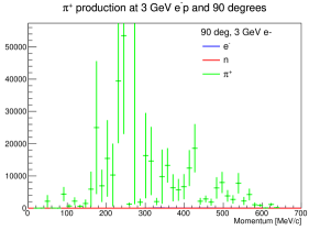
(d)

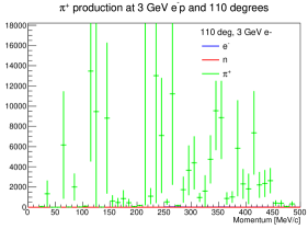
(e)

Figure 40: Number of electrons, neutrons, and $\pi^{+}$ directed towards the $5\times 5$ calorimeter arrays at $30\degree$, $50\degree$, $70\degree$, $90\degree$, and $110\degree$ during one day of running at the nominal luminosity for the reaction $e^{-}+p\rightarrow e^{-}+n+\pi^{+}$ at 3 GeV.

Appendix H Monte Carlo Simulation for $e^{+}+p\rightarrow e^{+}+p+\pi^{0}$ at 3 GeV

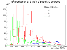
(a)

(b)

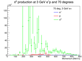
(c)

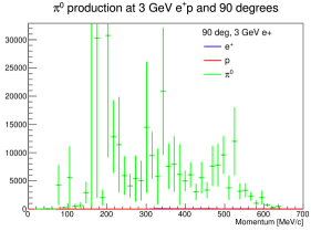
(d)

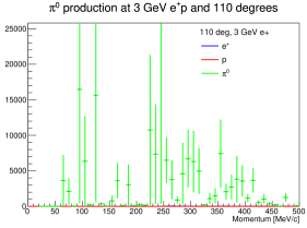
(e)

Figure 41: Number of positrons, protons, and $\pi^{0}$ directed towards the $5\times 5$ calorimeter arrays at $30\degree$, $50\degree$, $70\degree$, $90\degree$, and $110\degree$ during one day of running at the nominal luminosity for the reaction $e^{+}+p\rightarrow e^{+}+p+\pi^{0}$ at 3 GeV.

Appendix I Monte Carlo Simulation for $e^{+}+p\rightarrow e^{+}+n+\pi^{+}$ at 3 GeV

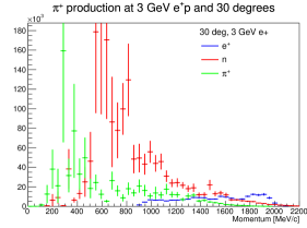
(a)

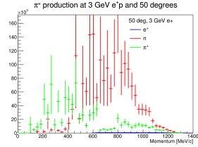
(b)

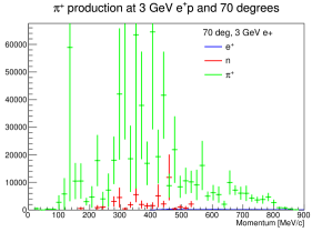
(c)

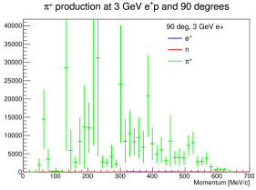
(d)

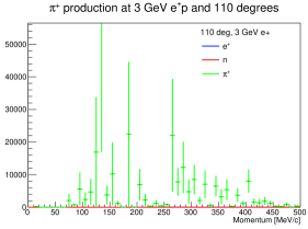
(e)

Figure 42: Number of positrons, neutrons, and $\pi^{+}$ directed towards the $5\times 5$ calorimeter arrays at $30\degree$, $50\degree$, $70\degree$, $90\degree$, and $110\degree$ during one day of running at the nominal luminosity for the reaction $e^{+}+p\rightarrow e^{+}+n+\pi^{+}$ at 3 GeV.

Appendix J Hydrogen Properties

Hydrogen normally exists as a diatomic molecule, H₂. The molecule occurs in two forms or allotropes: orthohydrogen, where the nuclear spins of the two atoms are parallel ($J=0,2,4,\dots$); and parahydrogen, where the nuclear spins are anti-parallel ($J=1,3,5,\dots$).

The concentrations of the two allotropes vary with temperature. At 80 K the concentration of each is roughly the same. At room temperature and above it is generally 75% orthohydrogen. At 19 K it is 99.75% parahydrogen. Various parameters are given in Table 9.

	Para-Equilibrium	Normal
Critical point
Temperature	32.976 K	33.19 K
Pressure	1.2928 MPa (12.759 atm)	1.315 MPa (12.98 atm)
Density	31.43 kg/m3 (15.59 mol/L)	30.12 kg/m3 (14.94 mol/L)
Normal boiling point
Temperature	20.268 K	20.39 K
Pressure	0.101325 MPa (1 atm)	0.101325 MPa (1 atm)
Density (liquid)	70.78 kg/m3 (35.11 mol/L)	71.0 kg/m3 (35.2 mol/L)
Density (vapor)	1.338 kg/m3 (0. 6636 mol/L)	1.331 kg/m3 (0.6604 mol/L)
Triple point
Temperature	13.803 K	13.957 K
Pressure	0.00704 MPa (0.0695 atm)	0.00720 MPa (0.0711 atm)
Density (solid)	86.50 kg/m3 (42.91 mol/L)	86.71 kg/m3 (43.01 mol/L)
Density (liquid)	77.03 kg/m3 (38.21 mol/L)	77.2 kg/m3 (38.3 mol/L)
Density (vapor)	0.126 kg/m3 (0.0623 mol/L)	0.130 kg/m3 (0.0644 mol/L)
Molecular Weight	2.01588

Table 9: Parameters for hydrogen

Figure 43: Cooling power of the cold head being considered for the TPEX liquid hydrogen target system.

Appendix K Lead Tungstate, PbWO₄, Properties

From the 2020 Particle Data Group Atomic and Nuclear Properties of Materials:

Density PbWO4	=	8.300 g$\cdot$cm-3
$2\times 2\times 20$ cm3 crystal	=	664.0 g
Molière radius	=	1.959 cm
Nuclear Interaction Length $\lambda_{\rm I}$	=	168.3 g$\cdot$cm-2
	=	20.28 cm
Radiation Length $X_{0}$	=	7.39 g$\cdot$cm-2
	=	0.8904 cm
Energy Loss $dE/dx$	=	1.229 MeV$\cdot$g${}^{-1}\cdot$cm2
	=	10.2 MeV$\cdot$cm-1

Appendix L Numbers Used for Calculations in this Proposal

Density LH2	=	0.07078 g$\cdot$cm-3
	=	4.2289$\times 10^{22}$ atoms$\cdot$cm-3
20 cm LH2 target	=	8.4578$\times 10^{23}$ atoms$\cdot$cm-2
40 nA on 20 cm LH2 target	=	2.1116$\times 10^{35}$ cm${}^{-2}\cdot$s${}^{-1}\cdot$sr-1
	=	2.1116$\times 10^{-4}$ fb${}^{-1}\cdot$s${}^{-1}\cdot$sr-1
$1.0\times 10^{7}$ fb	=	7.6018 events$\cdot$s-1 into 3.6 msr

References

- Janssens et al. [1966] T. Janssens, R. Hofstadter, E. B. Hughes, and M. R. Yearian, Phys. Rev. 142, 922 (1966).
- Berger et al. [1971] C. Berger, V. Burkert, G. Knop, B. Langenbeck, and K. Rith, Phys. Lett. 35B, 87 (1971).
- Litt et al. [1970] J. Litt et al., Phys. Lett. 31B, 40 (1970).
- Bartel et al. [1973] W. Bartel, F. W. Busser, W. r. Dix, R. Felst, D. Harms, H. Krehbiel, P. E. Kuhlmann, J. McElroy, J. Meyer, and G. Weber, Nucl. Phys. B58, 429 (1973).
- Andivahis et al. [1994] L. Andivahis et al., Phys. Rev. D50, 5491 (1994).
- Walker et al. [1994] R. C. Walker et al., Phys. Rev. D49, 5671 (1994).
- Christy et al. [2004] M. E. Christy et al. (E94110), Phys. Rev. C70, 015206 (2004), eprint nucl-ex/0401030.
- Qattan et al. [2005] I. A. Qattan et al., Phys. Rev. Lett. 94, 142301 (2005), eprint nucl-ex/0410010.
- Jones et al. [2000] M. K. Jones et al. (Jefferson Lab Hall A), Phys. Rev. Lett. 84, 1398 (2000), eprint nucl-ex/9910005.
- Pospischil et al. [2001] T. Pospischil et al. (A1), Eur. Phys. J. A12, 125 (2001).
- Gayou et al. [2001] O. Gayou et al., Phys. Rev. C64, 038202 (2001).
- Punjabi et al. [2005] V. Punjabi et al., Phys. Rev. C71, 055202 (2005), [Erratum: Phys. Rev.C71,069902(2005)], eprint nucl-ex/0501018.
- Crawford et al. [2007] C. Crawford et al., Phys. Rev. Lett. 98, 052301 (2007).
- Puckett et al. [2010] A. J. R. Puckett et al., Phys. Rev. Lett. 104, 242301 (2010), eprint 1005.3419.
- Ron et al. [2011] G. Ron et al. (Jefferson Lab Hall A), Phys. Rev. C84, 055204 (2011), eprint 1103.5784.
- Puckett et al. [2012] A. J. R. Puckett et al., Phys. Rev. C85, 045203 (2012), eprint 1102.5737.
- Henderson et al. [2017] B. S. Henderson et al. (OLYMPUS), Phys. Rev. Lett. 118, 092501 (2017), eprint 1611.04685.
- Blunden and Melnitchouk [2017] P. G. Blunden and W. Melnitchouk, Phys. Rev. C95, 065209 (2017), eprint 1703.06181.
- Bernauer et al. [2014] J. C. Bernauer et al. (A1), Phys. Rev. C90, 015206 (2014), eprint 1307.6227.
- Tomalak and Vanderhaeghen [2015] O. Tomalak and M. Vanderhaeghen, Eur. Phys. J. A51, 24 (2015), eprint 1408.5330.
- Rachek et al. [2015] I. A. Rachek et al., Phys. Rev. Lett. 114, 062005 (2015), eprint 1411.7372.
- Adikaram et al. [2015] D. Adikaram et al. (CLAS), Phys. Rev. Lett. 114, 062003 (2015), eprint 1411.6908.
- Bernauer et al. [2020] J. C. Bernauer et al. (2020), eprint 2008.05349.
- Kelly [2004] J. Kelly, Phys. Rev. C 70, 068202 (2004).
- Arrington [2004] J. Arrington, Phys. Rev. C 69, 032201 (2004), eprint nucl-ex/0311019.
- Arrington et al. [2007] J. Arrington, W. Melnitchouk, and J. Tjon, Phys. Rev. C 76, 035205 (2007), eprint 0707.1861.
- EWB [2017] (2017), URL https://www.physics.umass.edu/acfi/seminars-and-workshops/the-electroweak-box.
- Afanasev et al. [2017] A. Afanasev, P. G. Blunden, D. Hasell, and B. A. Raue, Prog. Part. Nucl. Phys. 95, 245 (2017), eprint 1703.03874.
- Blau [2017] S. K. Blau, Physics Today 70, 14 (2017).
- NST [2017] (2017), URL {http://nstar2017.physics.sc.edu/}.
- JPo [2017] (2017), URL {https://www.jlab.org/conferences/JPos2017/index.html}.
- Diener et al. [2019] R. Diener et al., Nucl. Instrum. Meth. A 922, 265 (2019), eprint 1807.09328.
- Roy et al. [2020] P. Roy, S. Corsetti, M. Dimond, M. Kim, L. L. Pottier], W. Lorenzon, R. Raymond, H. Reid, N. Steinberg, N. Wuerfel, et al., Nuclear Instruments and Methods in Physics Research Section A: Accelerators, Spectrometers, Detectors and Associated Equipment 949, 162874 (2020), ISSN 0168-9002, URL http://www.sciencedirect.com/science/article/pii/S0168900219312963.
- Group [2011] S. C. Group, Ch-110 series cryocoolers system configurations (2011), URL http://www.shicryogenics.com/products/specialty-cryocoolers/ch-110lt-30k-cryocooler-series.
- of America Inc. [2008] S. S. C. of America Inc., F-70h and f-70l helium compressors operating manual (2008).
- Gilman et al. [2016] R. Gilman et al., Technical Design Report for the Paul Scherrer Institute Experiment R-12-01.1: Studying the Proton “Radius” Puzzle with p Elastic Scattering (2016), URL http://www.physics.rutgers.edu/~rgilman/elasticmup/muse_tdr_new.pdf.
- Zhu et al. [1996] R. Y. Zhu, D. A. Ma, H. B. Newman, C. L. Woody, J. A. Kierstad, S. P. Stoll, and P. W. Levy, Nucl. Instrum. Meth. A376, 319 (1996).
- Zhu [2004] R. Y. Zhu, IEEE Trans. Nucl. Sci. 51, 1560 (2004).
- Neyret et al. [2000] D. Neyret et al., Nucl. Instrum. Meth. A443, 231 (2000), eprint hep-ex/9907047.
- Albrecht [2015] M. Albrecht (PANDA), J. Phys. Conf. Ser. 587, 012050 (2015).
- Pérez Benito et al. [2016] R. Pérez Benito, D. Khaneft, C. O’Connor, L. Capozza, J. Diefenbach, B. Gläser, Y. Ma, F. E. Maas, and D. Rodríguez Piñeiro, Nucl. Instrum. Meth. A 826, 6 (2016), eprint 1602.01702.
- Schmidt et al. [2018] A. Schmidt, C. O’Connor, J. C. Bernauer, and R. Milner, Nucl. Instrum. Meth. A877, 112 (2018), eprint 1708.04616.
- Abrahamyan et al. [2012] S. Abrahamyan et al., Phys. Rev. Lett. 108, 112502 (2012), eprint 1201.2568.
- Allison et al. [2015] T. Allison et al. (Qweak), Nucl. Instrum. Meth. A 781, 105 (2015), eprint 1409.7100.
- Denniston et al. [2020] A. Denniston et al. (2020), eprint 2004.10268.
- Hasell et al. [2009] D. Hasell et al., Nucl. Instrum. Meth. A603, 247 (2009).
- Collaboration et al. [2008] P. Collaboration, W. Erni, I. Keshelashvili, et al., Technical design report for panda electromagnetic calorimeter (emc) (2008), eprint 0810.1216.
- [48] T. Rostomyan et al., Timing detectors with sipm read-out for the muse experiment at psi, in preparation.
- Friederich et al. [2011] H. Friederich, G. Davatz, U. Hartmann, A. Howard, H. Meyer, D. Murer, S. Ritt, and N. Schlumpf, IEEE Transactions on Nuclear Science 58, 1652 (2011).
- Allison et al. [2016] J. Allison, K. Amako, J. Apostolakis, P. Arce, M. Asai, T. Aso, E. Bagli, A. Bagulya, S. Banerjee, G. Barrand, et al., Nuclear Instruments and Methods in Physics Research Section A: Accelerators, Spectrometers, Detectors and Associated Equipment 835, 186 (2016), ISSN 0168-9002, URL http://www.sciencedirect.com/science/article/pii/S0168900216306957.