Rotation Periods, Inclinations, and Obliquities of Cool Stars Hosting Directly Imaged Substellar Companions: Spin-Orbit Misalignments are Common

Abstract

The orientation between a star’s spin axis and a planet’s orbital plane provides valuable information about the system’s formation and dynamical history. For non-transiting planets at wide separations, true stellar obliquities are challenging to measure, but lower limits on spin-orbit orientations can be determined from the difference between the inclination of the star’s rotational axis and the companion’s orbital plane ($\Delta i$). We present results of a uniform analysis of rotation periods, stellar inclinations, and obliquities of cool stars (SpT $\gtrsim$ F5) hosting directly imaged planets and brown dwarf companions. As part of this effort, we have acquired new $v\sin i_{*}$ values for 22 host stars with the high-resolution Tull spectrograph at the Harlan J. Smith telescope. Altogether our sample contains 62 host stars with rotation periods, most of which are newly measured using light curves from the Transiting Exoplanet Survey Satellite. Among these, 53 stars have inclinations determined from projected rotational and equatorial velocities, and 21 stars predominantly hosting brown dwarfs have constraints on $\Delta i$. Eleven of these (52${}^{+10}_{-11}$% of the sample) are likely misaligned, while the remaining ten host stars are consistent with spin-orbit alignment. As an ensemble, the minimum obliquity distribution between 10–250 AU is more consistent with a mixture of isotropic and aligned systems than either extreme scenario alone—pointing to direct cloud collapse, formation within disks bearing primordial alignments and misalignments, or architectures processed by dynamical evolution. This contrasts with stars hosting directly imaged planets, which show a preference for low obliquities. These results reinforce an emerging distinction between the orbits of long-period brown dwarfs and giant planets in terms of their stellar obliquities and orbital eccentricities.

1 Introduction

Measurements of stellar obliquity—the orientation between a star’s spin axis and a planet’s orbital angular momentum vector—provide valuable clues about how planets form, migrate, and dynamically interact (Winn & Fabrycky 2015; Albrecht et al. 2022). In the absence of external perturbers, the axisymmetric collapse of a molecular cloud core is expected to result in mutual alignment between the stellar spin and the protoplanetary disk’s axis of rotation, which would then be inherited by any planets that form in the disk.

Many processes can disrupt this alignment and produce a wide range of stellar and planetary obliquities during and after the phase of planet formation. These mechanisms can act on the star, the planet, or the protoplanetary disk and include the influence of passing stars (Heller 1993; Batygin et al. 2020); secular torques from wide stellar and substellar companions (Fabrycky & Tremaine 2007; Batygin 2012; Anderson et al. 2016; Lai et al. 2018); and gravitational scattering with other planets (Chatterjee et al. 2008; Ford & Rasio 2008). Primordial misalignments of protoplanetary disks (both “intact” and “broken”) appear to be common, indicating that some planets probably form with substantial spin-orbit angles (e.g., Bate et al. 2010; Huber et al. 2013; Marino et al. 2015; Ansdell et al. 2020; Epstein-Martin et al. 2022). Even the Sun is misaligned by about 6$\arcdeg$ with respect to the solar system’s invariable plane, but the origin of this enigmatic offset continues to be debated (e.g., Adams 2010; Bailey et al. 2016; Spalding 2019).

Large transiting planets have provided a wealth of information about stellar obliquities, largely through individual and collective studies of Rossiter-McLaughlin measurements (Rossiter 1924; McLaughlin 1924; Queloz et al. 2000; Gaudi & Winn 2007). It is now clear that non-zero obliquities are common among field stars hosting short-period planets (Fabrycky & Winn 2009; Schlaufman 2010; Louden et al. 2021; Muñoz & Perets 2018), and especially those with temperatures above the Kraft break at $\approx$6250 K (Winn et al. 2010; Schlaufman 2010). As an ensemble, however, most compact multiplanet systems tend to have lower stellar obliquities (Albrecht et al. 2013; Morton & Winn 2014; Winn et al. 2017). A complex picture is emerging in which several mechanisms are probably responsible for tilting and in some contexts realigning the orbits of close-in planets over many different timescales (e.g., Morton & Johnson 2011; Albrecht et al. 2012; Dawson 2014).

Less, however, is known about stellar obliquities for systems hosting long-period companions. At wide separations, stellar obliquities can be used to provide clues about the formation and orbital evolution of companions amenable to direct imaging (Bowler 2016). In particular, planets and brown dwarfs have been discovered at separations spanning tens to thousands of AU and may originate from a combination of outward gravitational scattering (Boss 2006; Veras et al. 2009; Bailey & Fabrycky 2019); in situ formation in a disk via pebble accretion or disk instability (Durisen et al. 2007; Lambrechts & Johansen 2012); dynamical capture (Perets & Kouwenhoven 2012); or direct collapse from a fragmenting molecular cloud core (Bate 2012). There is growing evidence that most directly imaged planets within about one hundred AU are formed in a disk based on their eccentricity distributions (Bowler et al. 2020a), mass functions (Wagner et al. 2019), and demographic trends (Nielsen et al. 2019; Vigan et al. 2021). Spin-orbit angles (between the stellar spin axis and companion orbital plane) and spin-spin angles (between the spin axes of the host star and companion) can provide another unique perspective on the origin and orbital evolution of this population.

Figure 1: Orbital and rotational geometry relevant for obliquity constraints of stars hosting imaged companions. The observer is looking down from the $z$-axis. The $x$-$y$ plane is the plane of the sky, and the star is centered on the origin. The $x$-axis points north and the $y$-axis points east. Left: The inclination of the companion’s orbital plane, $i_{o}$, intersects the sky along the line of nodes, which is oriented by $\Omega_{o}$ from true north to the ascending node. In this configuration the orbital angular momentum vector $\overrightarrow{L_{o}}$ points in the hemisphere facing the observer, with $\overrightarrow{L_{o}}$ pointing toward the observer along the $z$ axis when $i_{o}$=0$\arcdeg$. Middle: The star’s orientation in space determines the inclination of its equatorial plane, $i_{*}$, and the position angle of its line of nodes. The sense of the stellar spin sets its rotational angular momentum vector $\overrightarrow{L_{*}}$ and the longitude of ascending node $\Omega_{*}$. Right: If only the inclinations $i_{o}$ and $i_{*}$ are measured, but not their true (or relative) orientations in the plane of the sky ($\Omega_{o}$ and $\Omega_{*}$), then each angular momentum vector can fall anywhere along nested cones opening toward or away from the observer. If $\Omega_{o}$ is known (point A₁, for example), but not $\Omega_{*}$, then the obliquity can be as small as $|i_{o}$–$i_{*}|$ (at B₁), can reach $i_{o}$ + $i_{*}$ for prograde orbits (B₂), or can be as large as $\pi-|i_{o}-i_{*}|$ (B₃) for retrograde orbits.

Measuring stellar obliquities is challenging at wide separations. The Rossiter-McLaughlin effect becomes less practical as a tool to study projected spin-orbit orientations because the geometric probability of a transit is lower, transit events are less frequent, and transit durations become longer; this explains why few systems with orbital periods beyond a few tens of days have had stellar obliquity measurements (Albrecht et al. 2022). Our strategy in this study is to use stellar rotation periods, projected rotational velocities, and stellar radii to infer the spin-orientation of stars hosting imaged substellar companions. The goal is to uniformly establish stellar inclinations for the full sample of host stars, then determine stellar obliquities for the subset of these with measurements of the orbital inclination from orbit monitoring. As a byproduct of this analysis, we also present rotation periods for 62 host stars, which can be used to refine the ages of these systems using gyrochronology.

This paper is organized as follows. In Section 2 we summarize the geometry and overall framework to constrain inclinations and obliquities for host stars of imaged companions. A description of our sample, new high-resolution spectroscopy, and Transiting Exoplanet Survey Satellite (TESS; Ricker et al. 2015) light curves are detailed in Section 3. Section 4 includes our $v\sin{i_{*}}$ measurements, periodicity analysis, stellar line-of sight inclinations, and obliquity constraints. The interpretation of our results and a discussion of sample biases can be found in Section 5. Our conclusions are summarized in Section 6.

2 Stellar Obliquity Geometry for Directly Imaged Companions

The problem of observationally measuring the angle between the stellar spin axis and a companion’s orbital plane, $\psi$, has a long history in the context of stellar binaries and the coplanarity of disks (e.g., Hale 1994; Watson et al. 2011). For clarity we briefly review the basic geometric setup of this problem as it applies to directly imaged companions.

Figure 1 shows the relevant orbital elements of a visual binary companion (left diagram) and the orientation of the spin axis of its host star (middle diagram). The observer is looking down along the $z$ axis toward the $x$-$y$ sky plane. The orbital plane of an imaged planet is characterized by its inclination $i_{o}$ with respect to the sky plane, which is equal to the angle between the $z$ axis and the orbital angular momentum vector $\overrightarrow{L_{o}}$, and the longitude of ascending node $\Omega_{o}$, defined from celestial north (here the $x$ axis) increasing eastward (toward the $y$ axis) to the line of nodes. $i_{o}$ spans 0–$\pi$ and $\Omega_{o}$ spans 0–2$\pi$. In general, orbit monitoring with relative astrometry results in an ambiguity between $\Omega_{o}$ and $\Omega_{o}$ + 180$\arcdeg$, which can be distinguished with radial velocities (RVs) of the companion (e.g., Snellen & Brown 2018; Ruffio et al. 2019; Ruffio et al. 2021) or its host star (e.g., Crepp et al. 2012; Bowler et al. 2018).

The setup is similar for the spinning star: its equatorial plane is inclined by $i_{*}$ from the sky plane, equal to the angle between the observer’s line of sight and the star’s rotational angular momentum vector $\overrightarrow{L_{*}}$. The direction in which $\overrightarrow{L_{*}}$ points is determined by its orientation on the sky, $\Omega_{*}$. With few exceptions for direct measurements of stellar oblateness (e.g., Belle 2012) and resolved rotation (Kraus et al. 2020), $\Omega_{*}$ is generally unknown.

The relationship between $i_{o}$, $\Omega_{o}$, $i_{*}$, and $\Omega_{*}$ can be derived by an observer-to-orbit coordinate system transformation (Fabrycky & Winn 2009) or via the spherical law of cosines (Glebocki & Stawikowski 1997):

$$\cos{\psi}=\cos{i_{o}}\cos{i_{*}}+\sin{i_{o}}\sin{i_{*}}\cos(\Omega_{o}-\Omega_{*})$$ (1)

For transiting planets, $i_{o}$ is known ($\approx$90$\arcdeg$) and the projected spin-orbit orientation $\Delta\Omega$ = $\Omega_{o}-\Omega_{*}$ (often denoted as $\lambda$) can be measured with the Rossiter-McLaughlin effect (Holt 1893; Rossiter 1924; McLaughlin 1924). In this case $i_{*}$ in general is unknown, and $\cos{\psi}$ $\approx$ $\sin{i_{*}}\cos(\lambda)$, so $\lambda$ is a lower limit on the true obliquity.

For directly imaged planets, $i_{o}$ can be measured through orbit monitoring. In some cases the inclination of the host star can be determined through asteroseismology (e.g., Zwintz et al. 2019) or the projected rotational velocity technique, which relies on knowing $v\sin{i_{*}}$, the rotation period $P_{\mathrm{rot}}$, and the stellar radius $R_{*}$ (Shajn & Struve 1929). This latter approach is the focus of this study and is possible for spotted stars whose rotational modulations manifest as periodic light curve variations.

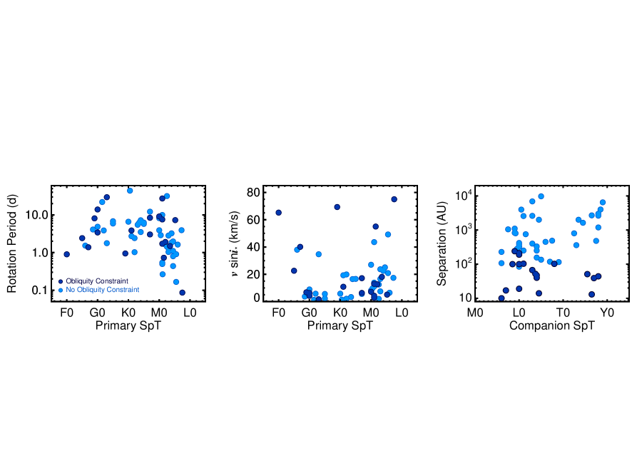
Figure 2: Overview of the host star spectral types and rotation periods (left), projected rotational velocities (middle), and companion spectral types and separations (right). Systems with stellar obliquity constraints are plotted in dark blue. Companions with obliquity constraints in this study reside within $\approx$250 AU where orbital motion is more readily detectable.

There is an important distinction between simple coplanarity of the orbital and stellar equatorial planes, versus genuine alignment of the orbital and rotational angular momentum vectors between the companion and the host star—the primary angle of interest in this study. When considering only coplanarity (which could include spin-orbit “anti-alignment”, or retrograde orbits) and both $i_{o}$ and $i_{*}$ are known (but not $\Delta\Omega$), the sum and absolute difference between the orbital and stellar inclinations provides boundaries on the true spin-orbit alignment:

$$|i_{o}-i_{*}|\leq\psi_{\mathrm{coplanar}}\leq i_{o}+i_{*}.$$ (2)

On the other hand, if one is concerned with angular momentum alignment in the system, and only $i_{o}$ and $i_{*}$ are known, there exists a broader range of possibilities for $\psi$ because the measurement of $i_{*}$ does not contain information about the sense of the spin. Depending on the direction of rotation, the spin angular momentum vector may be pointing toward the observer or away from the observer into the plane of the sky. In this case the constraint on $\psi$ becomes:

$$|i_{o}-i_{*}|\leq\psi_{\mathrm{true}}\leq\pi-|i_{o}-i_{*}|.$$ (3)

Regardless, if $i_{o}$ and $i_{*}$ differ then $\psi$ is non-zero and the system’s orbital and rotational planes are misaligned by at least $|i_{o}-i_{*}|$. However, if $i_{o}$ and $i_{*}$ are identical then the system is consistent with being aligned but the true obliquity may be much larger.

This is illustrated in the right-most diagram in Figure 1. If only $i_{o}$ and $i_{*}$ are known, the projection of the orbital and rotational angular momentum vectors will trace out nested cones with a degeneracy between the cones opening toward and away from the observer. If $i_{o}$ is fixed at point A₁, for example, and a stellar inclination $i_{*}$ is measured, the minimum value of $\psi$ will occur when $\Omega_{*}$=$\Omega_{o}$ at point B₁. If $\Omega_{*}$=$\Omega_{o}$ + 180$\arcdeg$ (B₂), $\psi$ can reach $i_{o}$ + $i_{*}$. But if $\overrightarrow{L_{*}}$ points away from the observer (residing on the lower cone opening in the $-z$ direction), $\Delta\Omega$ = 180$\arcdeg$ (B₃), and $\psi$ can reach a value as high as 180$\arcdeg$ – $|i_{o}-i_{*}|$. For instance, if $i_{o}$ = $i_{*}$ = 30$\arcdeg$, the orbital and rotational planes can be perfectly coincident ($\psi$ = 0$\arcdeg$) or misaligned by up to 60$\arcdeg$, and the spin-orbit angle can be misaligned by up to 120$\arcdeg$. This study focuses on measurements of the minimum misalignment, $\Delta i$ = $|i_{o}-i_{*}|$, for stars hosting directly imaged substellar companions.

3 Observations

3.1 Sample of Substellar Hosts

Our sample originates from a compilation of 177 stars hosting imaged substellar companions spanning a wide range of orbital separations. The list includes discoveries based on high-contrast imaging as well as wide common-proper motion companions identified from seeing-limited surveys. The compilation is assembled predominantly from the more focused lists in Deacon et al. (2014), Bowler (2016), and Bowler et al. (2020a), as well as additional systems identified more recently. The properties of the original parent sample are broad. Host star masses span the hydrogen burning limit up to supernova progenitors (Squicciarini et al. 2022); companions range in mass from 2 to about 75 $M_{\mathrm{Jup}}$ and orbital separations from a few AU to thousands of AU (Figure 2).

Table 1: Tull Spectrograph Radial Velocities and Projected Rotational Velocities

Name	UT Obs. Date	Exp. Time	RV	$\sigma_{\mathrm{RV}}$	$v\sin i$	$\sigma_{v\sin i}$	Standard	SpT
	(YYYY-MM-DD)	(s)	(m s-1)	(m s-1)	(km s-1)	(km s-1)	or Model	or $T_{\mathrm{eff}}$
1RXS J034231.8+121622	2022-02-21	1200	34.7	2.1	4.9	3.3	HD 119850	M1.5
1RXS J034231.8+121622	2022-02-21	1200	35.0	1.6	5.2	3.2	HD 119850	M1.5
1RXS J160929.1–210524	2019-06-26	1200	–8.4	1.1	8	2	HD 166620	K2
1RXS J160929.1–210524	2019-06-26	1200	–8.2	1.0	8.3	1.7	HD 166620	K2
2MASS J22362452+4751425	2019-06-17	1200	$\cdots$	$\cdots$	6.8	1.4	PHOENIX	4100 K
2MASS J22362452+4751425	2019-06-27	1200	–22.9	0.7	6.8	2.0	HD 173701	K0
2MASS J23513366+3127229	2019-07-31	1200	$\cdots$	$\cdots$	15	3	PHOENIX	3600 K
2MASS J23513366+3127229	2019-07-31	1200	$\cdots$	$\cdots$	15	4	PHOENIX	3600 K
51 Eri	2021-10-16	120	22.3	3.3	69	3	HD 207978	F2
51 Eri	2022-02-21	300	22.0	2.4	69	6	HIP 29396	F0
G 196-3	2019-04-01	1200	0.0	0.7	16.8	1.7	GJ388	M4.5
Gl 229	2021-10-16	800	4.8	0.5	4.5	1.4	HD 245409	K7
Gl 504	2019-03-31	300	$\cdots$	$\cdots$	9.2	1.7	PHOENIX	5900 K
Gl 504	2019-03-31	900	$\cdots$	$\cdots$	8.8	0.9	PHOENIX	5900 K
Gl 504	2019-03-31	900	$\cdots$	$\cdots$	9.0	1.0	PHOENIX	5900 K
Gl 504	2019-03-31	900	$\cdots$	$\cdots$	8.7	1.0	PHOENIX	5900 K
Gl 504	2022-02-21	300	–27.7	0.6	7.6	0.2	HD 141004	G0
Gl 758	2019-06-15	300	–22.2	0.4	5.1	0.4	HD 173701	K0
Gl 758	2019-06-17	600	$\cdots$	$\cdots$	5.4	2.3	PHOENIX	5300 K
Gl 758	2019-06-27	300	$\cdots$	$\cdots$	6.2	1.8	PHOENIX	5300 K
GSC 6214-210	2019-06-26	1200	–6.1	0.8	6.8	0.5	HD 166620	K2
GSC 6214-210	2019-06-26	1200	–6.0	0.9	6.6	0.5	HD 166620	K2
GU Psc	2019-07-31	1200	$\cdots$	$\cdots$	23	4	PHOENIX	3400 K
GU Psc	2019-07-31	1200	$\cdots$	$\cdots$	25	5	PHOENIX	3400 K
HD 1160	2019-06-15	600	$\cdots$	$\cdots$	96	10	PHOENIX	9800 K
HD 1160	2019-06-17	600	$\cdots$	$\cdots$	97	7	PHOENIX	9800 K
HD 1160	2019-07-31	300	$\cdots$	$\cdots$	95	7	PHOENIX	9800 K
HD 19467	2021-10-16	600	6.1	0.2	3.3	0.4	HD 187923	G0
HD 206893	2019-06-15	600	–13.0	2.3	33	3	HD 182572	G8
HD 206893	2019-06-17	600	$\cdots$	$\cdots$	34	3	PHOENIX	6600 K
HD 4747	2021-10-16	600	9.6	0.3	3.1	0.3	HD 4628	K2
HD 49197	2019-05-12	600	9.8	0.6	23.1	1.4	HD 122652	F8
HD 984	2019-06-17	600	$\cdots$	$\cdots$	38.7	2.5	PHOENIX	6300 K
HR 7672	2019-06-15	300	5.2	0.6	5.8	2.1	HD 173701	K0
HR 7672	2019-06-17	600	$\cdots$	$\cdots$	6.4	1.5	PHOENIX	5900 K
HR 7672	2019-06-27	300	5.3	0.4	4.1	1.8	HD 182488	G8
HR 8799	2019-06-15	300	$\cdots$	$\cdots$	43	5	PHOENIX	7200 K
HR 8799	2019-06-16	300	$\cdots$	$\cdots$	52	7	PHOENIX	7200 K
HR 8799	2019-07-31	60	$\cdots$	$\cdots$	38	5	PHOENIX	7200 K
$\kappa$ And	2019-06-15	300	$\cdots$	$\cdots$	182	24	PHOENIX	10800 K
$\kappa$ And	2019-06-17	300	$\cdots$	$\cdots$	183	35	PHOENIX	10800 K
$\kappa$ And	2019-07-31	45	$\cdots$	$\cdots$	173	28	PHOENIX	10800 K
Ross 458	2019-04-01	1200	–12.3	0.9	11.5	1.3	GJ388	M4.5
ROXs 12	2020-07-20	1200	–5.4	1.3	8.2	2.4	HD 157881	K5
ROXs 12	2020-07-20	1200	–5.8	1.9	8.5	2.6	HD 157881	K5

From this list we identify stars with rotation periods and $v\sin i_{*}$ measurements—either new in this work or previously published. When considering rotation periods, we restrict our analysis to spectral types of F5 or later to reduce confusion between rotation periods and stellar pulsations (e.g., Sepulveda et al. 2022). This is especially true of the intermediate-mass $\gamma$ Dor pulsators which span late-A to mid-F spectral types and have characteristic $g$-mode oscillation frequencies of a few hours to a few days (Kaye et al. 1999; Aerts 2021). Light curves and periodograms of stars in the remaining sample are further visually inspected for signs of pulsations.

Two exceptions are made to this spectral type cut. HIP 21152 is an F5 member of the Hyades with a recently discovered brown dwarf companion (Bonavita et al. 2022; Kuzuhara et al. 2022; Franson et al. 2022b). Its light curve periodogram shows significant peaks that are not integer harmonics of its strongest signal, and are therefore not likely to be caused by rotational modulation. We therefore remove this star from our sample.

51 Eri is a young F0 member of the $\beta$ Pic moving group with an imaged planet at 11 AU (Macintosh et al. 2015). Sepulveda et al. (2022) found the host to be a $\gamma$ Dor pulsator, casting doubt on previous rotation periods determined from light curves. However, they also find a plausible core rotation rate of 0.9${}^{+0.3}_{-0.1}$ d, so we include this star in our sample but recognize that detailed asteroseismic analysis using a longer time series is needed to more reliably constrain the rotation properties of this massive star.

Finally, all light curves with low-amplitude modulations are carefully examined on a case-by-case basis for signs that the variations might be instrumental rather than astrophysical in nature. Optical artifacts from bright sources and scattering from Earthshine can result in low-level changes that may mimic real signals. Our criteria for retaining light curves are that the signals must show clear and consistent periodic brightness changes that are evident from visual inspection, rotation periods must be shorter than half of the TESS sector baseline ($\lesssim$13 d for a single sector), and amplitudes must be substantially higher than the expected sensitivity floor for the target star brightness.

After implementing these cuts, our final sample for this study comprises 62 host stars with rotation periods, 53 of which also have projected rotational velocities and stellar radius determinations. These measurements are detailed in the following subsections and are summarized in Table 3.3 and Table 2. A Gaia color-magnitude diagram of host stars in our final sample is shown in Figure 3.

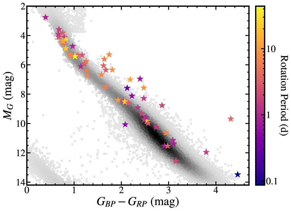
Figure 3: Gaia $G_{BP}$–$G_{RP}$ color-magnitude diagram of stars hosting imaged substellar companions in this study. With the exception of 51 Eri, the bluest star in the figure, we focus on cool stars of F5 and later to avoid confusion between stellar rotation and pulsations in our light curve analysis. Host stars are color-coded by rotation period and range from 0.08–44 d. Long rotation periods are either determined from multiple TESS sectors or are adopted from previous measurements in the literature.

3.2 High-Resolution Spectroscopy with the Tull Spectrograph

High-resolution optical spectra for 22 targets from our broader sample were obtained with the Tull Coudé Spectrograph (Tull et al. 1995) at McDonald Observatory’s 2.7-m Harlan J. Smith telescope between March 2019 and February 2022. The 1$\farcs$2 slit and E2 grating were used with the TS23 setup for all observations, which resulted in a resolving power of $R=\lambda/\delta\lambda\approx 60,000$. 56 échelle orders were simultaneously captured with the TK3 Tektronix CCD from 3870 Å to 10500 Å in (largely non-overlapping) segments ranging from 60 Å to 200 Å. On most nights we also observed several bright, slowly rotating RV and $v\sin i_{*}$ standards from Chubak et al. (2012) and Soubiran et al. (2018) spanning F through M spectral types. A summary of the observations can be found Table 1.

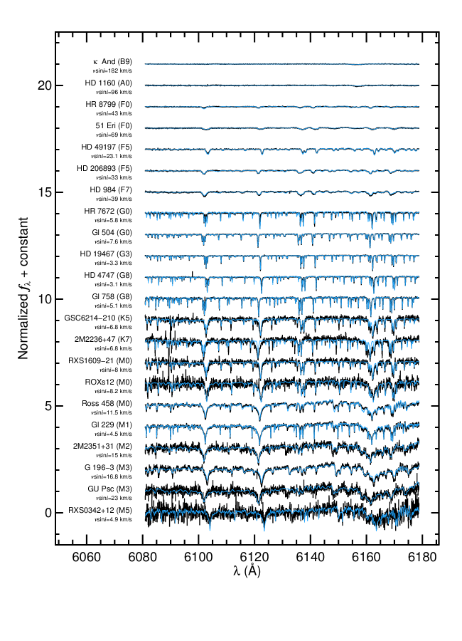
Figure 4: Example of a single order from our observations with the Tull high-resolution optical spectrograph (black). Stars are organized by decreasing spectral type from late-B to mid-M. Standard stars are overplotted in blue and have been broadened and shifted to match the measured radial and projected rotational velocities of the substellar host stars in our sample.

2-dimensional traces for the science observations are defined using a spectral flat field calibration frame taken on the same night. After bias subtraction and correction for known bad pixels, each curved spectral order is resampled to a linear two-dimensional trace using sub-pixel interpolation. Night sky lines are subtracted from each order using dispersed sky regions near the ends of the projected slit. Orders are optimally extracted following the method of Horne (1986), and fifth-order polynomial fits to the extracted flat spectra are used to remove the blaze function.

A wavelength solution is derived for each of the 56 orders using a ThAr emission line spectrum obtained on the same night and with the same setup as the science observations. A ThAr line list comprising a total of 9145 emission lines with documented relative line intensities was assembled spanning 3785 Å to 10507 Å from Lovis & Pepe (2007) (for $\lambda$ $<$ 6915 Å) and Murphy et al. (2007) (for $\lambda$ $>$ 6915 Å). For each order, a synthetic emission line spectrum was generated at the resolving power of the Tull spectrograph. To automate the process of mapping pixel values to wavelengths, we iteratively solved for the coefficients of a third-order polynomial model by maximizing the cross-correlation function between the observed spectral order and a “true” emission spectrum using the AMOEBA algorithm (Nelder & Mead 1965). With reasonable initial estimates for the coefficients, this approach performed well and the solution was visually verified for each order on each night.

3.3 TESS Light Curves

We used the lightkurve (Lightkurve Collaboration et al. 2018) package to download the 2-minute cadence Science Processing Operations Center (SPOC) Pre-search Data Conditioning Simple Aperture Photometry (PDCSAP) light curve (Smith et al. 2012; Stumpe et al. 2012; Stumpe et al. 2014; Jenkins et al. 2016) from the Mikulski Archive for Space Telescopes (MAST). Two targets (GJ 3305 and SDSS J130432.93+090713.7) were analyzed using their 30-minute Full Frame Images (FFIs), which were reduced by either the TESS-SPOC (Caldwell et al. 2020) or the MIT Quick-Look Pipeline (Huang et al. 2020) and manually retrieved from the MAST online portal.

All photometric measurements listed as NaN are removed. Individual TESS sector light curves are normalized by dividing both the flux and flux uncertainties by the median flux value of that sector. Each complete light curve is then compiled by stitching together these normalized sectors. Flares, transits, and other photometric outliers are removed by detrending the light curve with a high-pass Savitzky-Golay filter (Savitzky & Golay 1964) and only selecting data points in the original light curve that lie within one standard deviation of the flattened light curve. Note that because of flares and outlier photometric points, this threshold is typically larger than what it would be for pure Gaussian noise. Our period measurements (described below) are in good agreement whether or not we include this outlier rejection step.

For each processed light curve used in this study, we produce Generalized Lomb-Scargle (GLS) periodograms (Zechmeister & Kürster 2009) over the frequency range 0.0005–100.0 d^-1 (0.01–2000 days) to search for any periodic modulation that could be attributed to rotation. A Gaussian is fit to the highest periodogram peak and the resulting mean and standard deviation are adopted for the period and its uncertainty, respectively. For stars with multiple sectors separated by data gaps, aliasing due to the spectral window function causes a “fringe pattern” with a broad envelope for all periodogram peaks. In such cases, the Gaussian is fit to the envelope structure in order to reflect that spread. Each resulting light curve is visually inspected to ensure significant periodicities reflected astrophysical variations instead of spacecraft-related systematic oscillations, for example from optical artifacts or Earthshine. These can manifest as gradual low-amplitude variations, sharp discontinuities from spacecraft motion, and scattered light features which rise and fall in sync with the 13.7-day orbit. Period measurements are considered reliable if they show a single strong peak, a phase-folded light curve with consistent structure among phased curves, and a rotational modulation amplitude that is large compared to the limiting sensitivity of TESS for that target brightness. Finally, we limit adopted measurements to periods $\lesssim$13 d, which corresponds to half of the TESS sector baseline; instrumental systematics make it challenging to recover lower frequency signals in TESS light curves (e.g., Avallone et al. 2022).

Altogether 46 stars have light curves that appear to reflect true rotational modulation. They exhibit a wide range of characteristic behaviors—amplitudes with 20%-level variations (PDS 70); consistent, symmetric, sinusoid-like modulations (2MASS J02155892–0929121, CD–35 2722, and G 196-3); signs of dramatic and rapid starspot evolution (HD 130948, HD 16270, HD 49197, and HD 97334); double-peaked structure (2MASS J01225093–2439505 and PZ Tel); and beating patterns reflecting the superposition of two frequencies, most likely reflecting binarity or differential rotation (TWA 5 Aab). Full light curves, periodograms, and phased light curves are shown in Figures 20–27. Rotation periods and TESS sectors used in this analysis are listed in Table 3.3.

LP 261-75 reflects an interesting example of an M dwarf whose rotation period would have been interpreted incorrectly if only one TESS sector had been available. The periodogram of its full light curve from Sectors 21 and 48 shows two comparably strong peaks at 1.11 d and 2.23 d (Figure 25); one signal is clearly a harmonic of the true rotation period. This confusion is evident in reported photometric rotation period measurements of this star in the literature: Newton et al. (2016) and Irwin et al. (2018) find values of 2.219 d and 2.22 d, respectively, while Canto Martins et al. (2020) list a value of 1.105 $\pm$ 0.027 d. We therefore separately analyzed each individual sector light curve. The Sector 21 light curve shows a strong peak at 1.11 d with smooth modulations and consistent amplitudes. 712 days later marks the beginning of the next set of observations in Sector 48. In this sector the regular modulations occur with a periodicity of 2.23 d.

We interpret this longer modulation as the true rotation period. This “period-doubling” behavior is consistent with the following scenario: during the Sector 21 observations, two groups of starspots with comparable surface covering fractions may have been located on opposite sides of the spinning star with a longitudinal phase difference of $\sim$180$\arcdeg$. Typically this setup with two large groups of spots would produce a light curve with a double-peaked structure having two amplitudes, but here the similar spot sizes and 180$\arcdeg$ phase difference seem to have conspired to mimic a faster period in Sector 21, which only later could be differentiated from the true value when one group of spots evolved or disappeared. This phenomenon is different from typical rotation period confusion from photometric light curves, which are usually caused by sampling and windowing effects from insufficient cadence relative to the rotation period of the star. This is not the case for these fine 2-minute observations from TESS. Instead, LP 261-75

Table 2: Host Star Properties

Name	Host	Comp.	Disc.	Sep.	TESS	$P_{\mathrm{rot}}$	$\sigma_{P,\mathrm{tot}}$	$P_{\mathrm{rot}}$	$R_{*}$	$\sigma_{R_{*},\mathrm{tot}}$	$R_{*}$	$v\sin i$	$\sigma_{v\sin i}$	$v_{\mathrm{eq}}$	$\sigma_{v_{\mathrm{eq}}}$
	SpT	SpT	Ref.	(AU)	Sectors	(d)	(d)	Ref.	($R_{\odot}$)	($R_{\odot}$)	Ref.	(km s-1)	(km s-1)	(km s-1)	(km s-1)
1RXS J034231.8+121622	M5.2	L0	1	19	5; 42-44	7.3	0.3	72	0.35	0.03	86	5	2	2.4	0.2
1RXS J160929.1-210524	M0	L4	2	330	$\cdots$	8.2	0.4	73	1.3	0.2	86	8.2	1.3	8.10	1.1
2MASS J01033563-5515561	M5.5	L:	3	84	2; 29	0.1664	0.0003	72	0.45	0.02	75	21	2	140	6
2MASS J01225093-2439505	M3.5	L3.7	4	52	3; 30	1.493	0.017	72	0.37	0.03	86	18.1	0.5	12.4	0.94
2MASS J02155892-0929121	M2.5+M5+M8	$\cdots$	5	90	4	1.438	0.015	72	0.39	0.06	87	12.5	0.7	14	2
2MASS J02192210-3925225	M6	L4	6	156	3	1.63	0.02	72	0.27	0.02	86	6.5	0.4	8.3	0.6
2MASS J04372171+2651014	M4	L7	7	118	43; 44	1.84	0.02	72	0.84	0.11	88	22.54	0.14	23	3
2MASS J16103196-1913062	K7	M9	8	828	$\cdots$	12.2	0.7	74	1.2	0.2	86	5.6	1.7	5.1	0.8
2MASS J23513366+3127229	M2	L0	9	100	$\cdots$	1.92	0.02	75	0.48	0.04	86	12.7	0.7	12.5	0.96
51 Eri	F0	T6.5	10	13	5; 32	0.9	0.2	76	1.666	0.005	89	65.2	0.6	90	30
AB Pic	K1	L0	11	190	1-13; 27-39	3.9	0.08	72	1.02	0.097	86	10.87	0.08	13.4	1.3
ASAS J212528-8138.5	M1	L3	12; 13	6900	13; 27; 39	0.542	0.002	72	0.67	0.05	86	43.6	1.2	63	5
BD+21 2486AB	K5+M4	L5	14; 15	9708	23; 50	6.3	0.3	72	0.72	0.09	86	$\cdots$	$\cdots$	5.8	0.8
BD+21 55	K2	L0.5	16	3970	$\cdots$	1.026	0.006	75	0.79	0.07	86	2.1	1.0	39	4
CD-35 2722	M1	L3	17	67	6; 32; 33	1.717	0.018	72	0.56	0.04	86	13.0	0.4	16.5	1.2
FU Tau	M7.25	M9.2	18	800	43; 44	3.93	0.09	72	1.40	0.10	75	17.4	0.3	18.0	1.4
FW Tau AB	M5.5	early-L	19	330	43; 44	0.907	0.005	72	1.28	0.11	75	49.2	0.7	71	6
G 196-3	M3	L3	20	400	21; 48	1.315	0.013	72	0.52	0.04	86	16.6	1.1	20	2
G 203-50	M4.5	L5	21	135	25; 26; 51; 53	1.98	0.02	72	0.164	0.013	86	$\cdots$	$\cdots$	4.2	0.3
G 204-39	M2.5	T6.5	22; 23	2685	$\cdots$	32	4	77	0.41	0.03	86	2.000	1.1	0.648	0.11
GJ 3305 AB	M1.1	T6.5	24	$\cdots$	5; 32 (FFI)	0.2657	0.0005	72	0.49	0.08	86	11.3	0.3	90	20
Gl 229	M1	T7	25	39	$\cdots$	27	3	78	0.55	0.06	86	2.8	0.4	1.0	0.2
Gl 504	G0	late-T	26	44	23; 50	3.42	0.09	72	1.35	0.04	90	6.3	0.1	20	0.8
GQ Lup	K7	L1	27	103	$\cdots$	8.4	0.5	79	1.7	0.2	91	6.34	0.07	10.2	1.3
GSC 00568-01752	M2	L3+L5	28; 29	2600	42	1.63	0.02	72	0.41	0.03	86	$\cdots$	$\cdots$	12.7	0.98
GSC 06214-00210	M1	M9	30	240	$\cdots$	7.6	0.3	74	0.91	0.1	86	4.29	0.05	6.0	0.7
GSC 08047-00232	K2	M9.5	31; 32	279	2; 3; 29; 30	2.42	0.04	72	0.90	0.09	86	19.9	0.6	19	2
GU Psc	M3	T3.5	33	2000	17; 42; 43	1.038	0.007	72	0.45	0.03	86	23.7	1.8	22	2
HD 116402	G3	M6	34	228	38	1.78	0.02	72	1.40	0.12	86	34.7	1.0	40	4
HD 129683	F6	M6	34	107	11; 38	1.53	0.02	72	1.42	0.12	86	38	3	47	4
HD 130948	F9	L4+L4	35	47	24; 50; 51	8.1	0.4	72	1.02	0.08	86	6.8	0.9	6.4	0.6
HD 16270	K3.5	L1	36	250	4; 30; 31	6.2	0.2	72	0.69	0.07	86	3.34	0.07	5.6	0.6
HD 19467	G3	T5.5	37	51	$\cdots$	30	4	80	1.30	0.05	92	1.68	0.08	2.2	0.3
HD 203030	K0	L7.5	38	487	15	6.6	0.3	72	0.88	0.08	86	5.8	0.12	6.7	0.7
HD 3651	K0.5	T7.5	39; 40	480	$\cdots$	44	7	81	0.87	0.07	86	1.4	0.2	1.0	0.2
HD 37216	G5	L1.5	16	753	19	6.8	0.3	72	0.85	0.07	86	5.6	1.7	6.3	0.6
HD 49197	F5	L4	41	40	20	2.4	0.3	72	1.12	0.09	86	22.6	1.0	23	3
HD 65486	K4	T4.5	42	1630	7; 8; 34	7.2	0.4	72	0.65	0.07	86	$\cdots$	$\cdots$	4.6	0.6
HD 8291	G5	L1+T3	16	2570	42; 43	5.9	0.2	72	0.89	0.07	86	2.25	1.1	7.6	0.7
HD 97334	G2	L4.5+L6	43; 44	2000	22; 48	3.87	0.12	72	1.05	0.09	86	5.8	0.5	13.7	1.3
HD 984	F7	M6	45	10	3; 42	1.39	0.02	72	1.15	0.098	86	40.1	1.0	42	4
HIP 70319	G1.5	T8	46	2630	$\cdots$	22	2	81	0.93	0.08	86	1.3	0.4	2.1	0.3
HN Peg	G0	T2.5	47	800	$\cdots$	4.9	0.1	82	1.01	0.09	86	8.92	0.08	10.5	0.98
HR 7672	G0	L4.5	48	14	$\cdots$	14	1	82	1.07	0.09	86	4.2	0.7	3.9	0.4
ksi UMa	F8.5+G2	T8.5	49	4000	22	4.10	0.12	72	1.01	0.11	86	3.7	1.4	12.4	1.4
L 34-26	M3	T9	50; 51	6471		2.83	0.04	72	0.39	0.03	86	7.5	0.4	6.9	0.5
LkCa 15	K5	$\cdots$	52	20	$\cdots$	5.77	0.18	83	1.6	0.2	93	16.6	0.2	14	2
LP 261-75	M4.5	L6	53; 54	450	21; 48	1.107	0.009	72	0.31	0.02	86	$\cdots$	$\cdots$	14.0	1.1
LP 903-20	M4	L4	55	250	35; 36	3.24	0.07	72	0.24	0.02	86	$\cdots$	$\cdots$	3.7	0.3
PDS 70	K7	$\cdots$	56	22	11	3.03	0.07	72	1.3	0.2	94	17.16	0.16	21	3
PM J02133+3648	M4.5+M6.5	T3	57	360	18	0.439	0.002	72	0.221	0.011	95	25.1	1.1	25.5	1.3
PZ Tel	G9	M7	58; 59	17	13	0.948	0.007	72	1.26	0.12	86	69.3	0.7	67	6
Ross 458 AB	M0.5+M7	T8	60; 61	1190	23; 50	2.89	0.06	72	0.56	0.04	86	9.8	0.3	9.8	0.8
ROXs 12	M0	L0	19	210	$\cdots$	9.1	0.6	84	1.14	0.07	96	7.21	0.07	6.3	0.6
RX J1602.8-2401B	K4	M7.5	8	1047	$\cdots$	3.51	0.07	85	1.2	0.2	97	16.5	1.3	18	3
SDSS J130432.93+090713.7	M4.5	L0	62	374	23 (FFI)	0.799	0.004	72	0.27	0.02	86	$\cdots$	$\cdots$	17.2	1.3
SR 12 AB	M0	M9	63	1100	$\cdots$	3.92	0.08	74	1.5	0.2	75	27	11	19	2
TWA 5 Aab	M1.5	M8.5	64; 65	100	10; 36	0.730	0.004	72	0.89	0.10	75	55.0	2.5	62	7
TYC 8984-2245-1	K1	L9	66	115	10; 11; 37; 38	2.73	0.05	72	1.11	0.11	86	19.3	0.5	21	2
TYC 8998-760-1	K3	L0; L7.5	67	320	11	5.5	0.2	72	1.02	0.11	86	$\cdots$	$\cdots$	9.42	1.1
UCAC4 070-020389	M1	L0	68; 69	418	11; 12	10	0.6	72	0.55	0.04	86	$\cdots$	$\cdots$	2.8	0.3
VHS J125601.92-125723.9 AB	M7.5	L8	70	102	10; 37	0.0866	0.001	72	0.17	0.06	98	75	3	100	30
Wolf 1130	sdM1+WD	T8	71	3000	15; 16; 41; 54	0.497	0.002	72	0.31	0.02	86	13.9	1.6	31	2

References. — (1) Bowler et al. (2015a); (2) Lafrenière et al. (2008); (3) Delorme et al. (2013); (4) Bowler et al. (2013); (5) Bowler et al. (2015b); (6) Artigau et al. (2015); (7) Gaidos et al. (2021); (8) Kraus & Hillenbrand (2009); (9) Bowler et al. (2012); (10) Macintosh et al. (2015); (11) Chauvin et al. (2005); (12) Reid et al. (2008); (13) Deacon et al. (2016); (14) Gomes et al. (2013); (15) Cruz et al. (2003); (16) Deacon et al. (2014); (17) Wahhaj et al. (2011); (18) Luhman et al. (2009); (19) Kraus et al. (2014a); (20) Rebolo et al. (1998); (21) Radigan et al. (2008); (22) Knapp et al. (2004); (23) Faherty et al. (2010); (24) Feigelson et al. (2006); (25) Nakajima et al. (1995); (26) Kuzuhara et al. (2013); (27) Neuhäuser et al. (2005); (28) Geballe et al. (2002); (29) Allers et al. (2010); (30) Ireland et al. (2011); (31) Chauvin et al. (2003); (32) Neuhäuser et al. (2003); (33) Naud et al. (2014); (34) Janson et al. (2012); (35) Potter et al. (2002); (36) Gizis et al. (2001); (37) Crepp et al. (2014); (38) Metchev & Hillenbrand (2006); (39) Mugrauer et al. (2006); (40) Liu et al. (2007); (41) Metchev & Hillenbrand (2004); (42) Deacon et al. (2012); (43) Kirkpatrick et al. (2001); (44) Bouy et al. (2003); (45) Meshkat et al. (2015); (46) Pinfield et al. (2012); (47) Luhman et al. (2007); (48) Liu et al. (2002); (49) Wright et al. (2013); (50) Kirkpatrick et al. (2011); (51) Zhang et al. (2021); (52) Kraus & Ireland (2012); (53) Kirkpatrick et al. (2000); (54) Reid & Walkowicz (2006); (55) Seifahrt et al. (2005); (56) Keppler et al. (2018); (57) Deacon et al. (2017); (58) Biller et al. (2010); (59) Mugrauer et al. (2010); (60) Goldman et al. (2010); (61) Scholz (2010); (62) Zhang et al. (2010); (63) Kuzuhara et al. (2011); (64) Lowrance et al. (1999); (65) Webb et al. (1999); (66) Bohn et al. (2021); (67) Bohn et al. (2020a); (68) Phan‐Bao et al. (2008); (69) Kendall et al. (2007); (70) Gauza et al. (2015); (71) Mace et al. (2013); (72) This work; (73) Mellon et al. (2017); (74) Rebull et al. (2018); (75) Oelkers et al. (2018); (76) Sepulveda et al. (2022); (77) Hartman et al. (2011); (78) Suarez Mascareno et al. (2016); (79) Donati et al. (2012); (80) Maire et al. (2020); (81) Baliunas et al. (1996); (82) Donahue et al. (1996); (83) Rodriguez et al. (2017); (84) Bowler et al. (2017); (85) Jayasinghe et al. (2018); (86) Stassun et al. (2019); (87) Stassun et al. (2018); (88) Gaidos et al. (2021); (89) Simon & Schaefer (2011); (90) Bonnefoy et al. (2018); (91) Donati et al. (2012); (92) Wood et al. (2019); (93) Davies et al. (2014); (94) Müller et al. (2018); (95) Muirhead et al. (2018); (96) Bowler et al. (2017); (97) Montalto et al. (2021); (98) Sebastian et al. (2021).

illustrates a (probably rare) instance of bias that can arise if only a single sector is available, which applies to 13 of the 62 host stars with rotation periods in our sample. Note that the deep 1.882-day transit events from LP 261-75 C (Irwin et al. 2018) were removed from the light curves for this analysis. These small regular gaps do not impact the results.

4 Results

4.1 New Projected Rotational and Radial Velocities

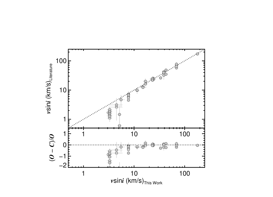
Figure 5: Comparison between $v\sin i_{*}$ values from this work and those from the literature for the same star. The dotted line is a 1:1 relationship. Above about 6 km s^-1, the agreement is good, but our $v\sin i_{*}$ values derived through cross correlation with slowly rotating standard stars are generally overestimated for low projected rotational velocities. The bottom panel shows fractional residuals.

Stars that we observed with the Tull Spectrograph range in spectral type from B9 to M5. Projected rotational velocities are determined by either applying a rotational broadening kernel to spectra of slowly rotating RV standards, or by broadening an appropriate model spectrum from the PHOENIX-ACES grid (Husser et al. 2013). Orders with low SNR, strong telluric lines, or few absorption lines (for early-type stars) were avoided. This typically resulted in 20–40 good orders. When using the empirical standards as a reference template, we first cross correlate every standard spectrum observed on the same night with each order of the science spectrum. The resulting individual cross-correlation functions (CCFs) for a particular standard are summed and the reference spectrum that results in the highest CCF value is adopted for the broadening analysis. Each order of the template spectrum is then sequentially broadened through a fine grid of $v\sin i_{*}$ values spanning 0 to 200 km/s with a rotational kernel following Gray (2005). A new CCF is computed for each $v\sin i_{*}$ value, and the broadening kernel resulting in the highest CCF peak for that order is added in quadrature with the measured $v\sin i_{*}$ value of the standard star. This is typically obtained from the compilation of projected rotational velocities by Glebocki & Gnacinski (2005); most of the standards we used have $v\sin i_{*}$ values below 3 km s^-1 for G, K, and M dwarfs and below 10 km s^-1 for F stars. The final adopted projected rotational velocity is then derived from the robust mean and standard deviation of the $v\sin i_{*}$ measurements for each individual order following the procedure in Beers et al. (1990). Uncertainties generally scale with the $v\sin i_{*}$ value but most are measured at the $\sigma_{v\sin i_{*}}$/$v\sin i_{*}$ $\sim$ 5–30% level.

This procedure also results in an instantaneous RV relative to the RV standard. A barycentric correction is applied following the approach in Stumpff (1980), then an absolute RV is computed using the RV of the standard. The total uncertainty is determined from the quadrature sum of our measured relative RV and the published uncertainty for the standard star. Although these measurements are not the primary focus of this study, we report RVs alongside $v\sin i_{*}$ values in Table 1.

On nights when an appropriate slowly rotating standard was not observed, or for early-type stars for which fewer standards are available, we used solar-metallicity synthetic spectra from the PHOENIX-ACES model atmosphere grid to determine projected rotational velocities. Model effective temperatures were chosen to the nearest 100 K (for $T_{\mathrm{eff}}$ $<$ 7000 K) or 200 K (for $T_{\mathrm{eff}}$ $\geq$ 7000 K) using the SpT–$T_{\mathrm{eff}}$ scale from Pecaut & Mamajek (2013). The models were first smoothed with a Gaussian kernal to the resolving power of the Tull spectrograph, trimmed to the wavelength range of the individual orders, and resampled onto the same wavelength grid as the science spectra. The same procedure for assessing rotational broadening is carried out for the models as for the standard star observations described above. Fewer orders were generally used for the B, A, and F stars as many orders for these early-type stars lacked lines altogether. $v\sin i_{*}$ values are determined separately for each order and then a robust mean and standard deviation are computed. Model effective temperatures are listed with the $v\sin i_{*}$ results in Table 1. Examples of spectra and broadened templates (both empirical and from model spectra) for a single order are shown in Figure 4.

We compiled previously determined $v\sin i_{*}$ values for targets in Table 1 to assess how our measurements compare with those in the literature (see Appendix D and

Table 3: Stellar Inclinations and Minimum Obliquities

Name	$i_{*}$			$i_{o}$		$\Delta i_{*}$			$P(\Delta i>10\arcdeg)$	Misaligned?
	MAP	Median	95.4% C.I.	Median	Ref.	MAP	Median	95.4% C.I.
	($\arcdeg$)	($\arcdeg$)	($\arcdeg$)	($\arcdeg$)		($\arcdeg$)	($\arcdeg$)	($\arcdeg$)
1RXS J034231.8+121622	90.0	66.5${}^{+23.4}_{-10.8}$	27.6–90.0	79.6${}^{+6.8}_{-5.5}$	1	2.5	26.7${}^{+12.4}_{-26.7}$	0.0–76.0	0.803	No Evidence
1RXS J160929.1-210524	90.0	71.8${}^{+18.2}_{-7.3}$	47.5–90.0	$\cdots$	$\cdots$	$\cdots$	$\cdots$	$\cdots$	$\cdots$	$\cdots$
2MASS J01033563-5515561	8.9	8.9${}^{+0.9}_{-1.3}$	6.9–11.0	$\cdots$	$\cdots$	$\cdots$	$\cdots$	$\cdots$	$\cdots$	$\cdots$
2MASS J01225093-2439505	90.0	85.9${}^{+4.1}_{-2.0}$	78.1–90.0	103.4${}^{+7.7}_{-9.2}$	2	9.5	14.2${}^{+5.8}_{-13.7}$	0.0–49.2	0.677	No Evidence
2MASS J02155892-0929121	66.4	69.1${}^{+15.1}_{-12.6}$	48.3–89.9	$\cdots$	$\cdots$	$\cdots$	$\cdots$	$\cdots$	$\cdots$	$\cdots$
2MASS J02192210-3925225	51.7	54.4${}^{+6.9}_{-10.0}$	39.2–77.8	$\cdots$	$\cdots$	$\cdots$	$\cdots$	$\cdots$	$\cdots$	$\cdots$
2MASS J04372171+2651014	77.3	73.9${}^{+15.7}_{-6.3}$	55.4–89.9	$\cdots$	$\cdots$	$\cdots$	$\cdots$	$\cdots$	$\cdots$	$\cdots$
2MASS J16103196-1913062	90.0	68.7${}^{+21.3}_{-9.1}$	36.9–90.0	$\cdots$	$\cdots$	$\cdots$	$\cdots$	$\cdots$	$\cdots$	$\cdots$
2MASS J23513366+3127229	90.0	77.7${}^{+12.3}_{-5.0}$	61.3–90.0	127.1${}^{+12.0}_{-15.9}$	1	39.5	38.6${}^{+17.3}_{-22.5}$	0.0–75.0	0.920	Likely
51 Eri	44.1	53.5${}^{+13.2}_{-19.3}$	31.9–87.6	144${}^{+8}_{-8}$	3	0.0	54.4${}^{+28.3}_{-54.2}$	0.0–110.5	0.854	No Evidence
AB Pic	54.4	58.5${}^{+7.7}_{-12.0}$	43.1–84.5	90${}^{+12}_{-12}$	4	32.4	30.1${}^{+15.5}_{-16.4}$	0.0–55.3	0.888	Likely
ASAS J212528-8138.5	44.0	45.1${}^{+4.1}_{-5.5}$	36.2–56.4	$\cdots$	$\cdots$	$\cdots$	$\cdots$	$\cdots$	$\cdots$	$\cdots$
BD+21 55	3.7	3.8${}^{+1.2}_{-1.6}$	1.1– 6.6	$\cdots$	$\cdots$	$\cdots$	$\cdots$	$\cdots$	$\cdots$	$\cdots$
CD-35 2722	52.2	54.4${}^{+5.6}_{-8.5}$	41.5–74.1	150.8 ${}^{+20.7}_{-14.5}$	1	35.5	54.8${}^{+36.0}_{-54.6}$	0.0–118.2	0.903	Likely
FU Tau	75.0	75.8${}^{+12.8}_{-6.3}$	60.7–89.9	$\cdots$	$\cdots$	$\cdots$	$\cdots$	$\cdots$	$\cdots$	$\cdots$
FW Tau AB	43.6	44.9${}^{+4.4}_{-5.9}$	35.4–57.6	$\cdots$	$\cdots$	$\cdots$	$\cdots$	$\cdots$	$\cdots$	$\cdots$
G 196-3	56.1	60.0${}^{+8.8}_{-12.2}$	43.9–86.1	$\cdots$	$\cdots$	$\cdots$	$\cdots$	$\cdots$	$\cdots$	$\cdots$
G 204-39	90.0	64.0${}^{+25.9}_{-11.7}$	23.0–90.0	$\cdots$	$\cdots$	$\cdots$	$\cdots$	$\cdots$	$\cdots$	$\cdots$
GJ 3305 AB	6.9	7.4${}^{+1.0}_{-1.7}$	4.9–10.9	$\cdots$	$\cdots$	$\cdots$	$\cdots$	$\cdots$	$\cdots$	$\cdots$
Gl 229	90.0	79.4${}^{+10.5}_{-5.0}$	59.7–90.0	5.50${}^{+0.16}_{-0.16}$	5	85.4	84.5${}^{+15.3}_{-16.2}$	52.6–114.8	1.00	Yes
Gl 504	18.4	18.5${}^{+0.7}_{-0.9}$	16.9–20.1	141.4${}^{+7.5}_{-10.7}$	1	120.5	97.3${}^{+29.7}_{-82.7}$	0.0–140.7	0.910	Likely
GQ Lup	38.3	40.9${}^{+5.9}_{-8.3}$	28.2–62.2	61.4${}^{+7.2}_{-5.9}$	6	77.7	38.9${}^{+44.3}_{-24.3}$	0.0–92.3	0.896	Likely
GSC 06214-00210	45.2	48.5${}^{+6.6}_{-10.1}$	33.9–73.9	114.4${}^{+8.9}_{-12.2}$	7	20.5	39.5${}^{+29.7}_{-31.7}$	0.0–94.6	0.865	Likely
GSC 08047-00232	90.0	79.0${}^{+10.9}_{-4.8}$	63.2–90.0	$\cdots$	$\cdots$	$\cdots$	$\cdots$	$\cdots$	$\cdots$	$\cdots$
GU Psc	90.0	79.1${}^{+10.8}_{-4.9}$	62.4–90.0	$\cdots$	$\cdots$	$\cdots$	$\cdots$	$\cdots$	$\cdots$	$\cdots$
HD 116402	60.7	65.4${}^{+9.5}_{-12.9}$	50.3–89.1	$\cdots$	$\cdots$	$\cdots$	$\cdots$	$\cdots$	$\cdots$	$\cdots$
HD 129683	54.7	59.0${}^{+9.5}_{-13.4}$	41.9–86.5	$\cdots$	$\cdots$	$\cdots$	$\cdots$	$\cdots$	$\cdots$	$\cdots$
HD 130948	90.0	75.1${}^{+14.7}_{-6.4}$	53.4–90.0	105${}^{+4}_{-4}$	8	0.0	17.7${}^{+8.5}_{-17.5}$	0.0–47.2	0.706	No Evidence
HD 16270	36.4	37.9${}^{+4.2}_{-6.1}$	28.4–50.7	$\cdots$	$\cdots$	$\cdots$	$\cdots$	$\cdots$	$\cdots$	$\cdots$
HD 19467	49.4	54.9${}^{+9.9}_{-14.4}$	36.9–85.2	129.8${}^{+6.6}_{-6.6}$	9	0.0	40.7${}^{+28.5}_{-40.5}$	0.0–90.3	0.745	No Evidence
HD 203030	60.0	65.3${}^{+10.3}_{-13.7}$	49.5–89.6	$\cdots$	$\cdots$	$\cdots$	$\cdots$	$\cdots$	$\cdots$	$\cdots$
HD 3651	90.0	77.0${}^{+12.9}_{-5.9}$	55.5–90.0	$\cdots$	$\cdots$	$\cdots$	$\cdots$	$\cdots$	$\cdots$	$\cdots$
HD 37216	74.4	65.2${}^{+24.8}_{-9.6}$	34.1–90.0	$\cdots$	$\cdots$	$\cdots$	$\cdots$	$\cdots$	$\cdots$	$\cdots$
HD 49197	75.0	72.8${}^{+16.7}_{-6.7}$	53.6–90.0	97.6${}^{+4.7}_{-8.6}$	1	4.5	18.4${}^{+8.1}_{-18.0}$	0.0–52.1	0.734	No Evidence
HD 8291	20.9	22.2${}^{+7.7}_{-9.8}$	5.7–41.1	$\cdots$	$\cdots$	$\cdots$	$\cdots$	$\cdots$	$\cdots$	$\cdots$
HD 97334	25.3	25.8${}^{+3.0}_{-4.1}$	19.2–33.5	$\cdots$	$\cdots$	$\cdots$	$\cdots$	$\cdots$	$\cdots$	$\cdots$
HD 984	72.8	74.3${}^{+12.1}_{-8.8}$	58.2–89.9	120.8${}^{+1.7}_{-1.7}$	10	12.6	30.8${}^{+16.6}_{-21.4}$	2.2–58.0	0.838	Likely
HIP 70319	41.2	47.8${}^{+15.6}_{-21.0}$	22.2–88.2	$\cdots$	$\cdots$	$\cdots$	$\cdots$	$\cdots$	$\cdots$	$\cdots$
HN Peg	57.9	62.5${}^{+8.5}_{-12.5}$	47.1–87.1	$\cdots$	$\cdots$	$\cdots$	$\cdots$	$\cdots$	$\cdots$	$\cdots$
HR 7672	90.0	73.7${}^{+16.2}_{-7.0}$	49.7–90.0	97.4${}^{+0.4}_{-0.4}$	11	0.0	16.6${}^{+7.6}_{-16.2}$	0.0–43.2	0.697	No Evidence
$\kappa$ And	30.1	30.1${}^{+4.0}_{-4.0}$	22.1–38.1	139.1${}^{+13.8}_{-18.4}$	1	0.0	72.4${}^{+31.0}_{-72.4}$	0.0–133.3	0.822	No Evidence
ksi UMa	19.6	20.7${}^{+6.4}_{-7.9}$	7.1–36.3	$\cdots$	$\cdots$	$\cdots$	$\cdots$	$\cdots$	$\cdots$	$\cdots$
L 34-26	90.0	80.2${}^{+9.7}_{-4.3}$	65.2–90.0	$\cdots$	$\cdots$	$\cdots$	$\cdots$	$\cdots$	$\cdots$	$\cdots$
LkCa 15	90.0	79.8${}^{+10.1}_{-4.6}$	63.7–90.0	$\cdots$	$\cdots$	$\cdots$	$\cdots$	$\cdots$	$\cdots$	$\cdots$
PDS 70	54.7	60.4${}^{+9.9}_{-14.7}$	43.8–88.2	132.8${}^{+3.0}_{-3.0}$	12	1.4	43.2${}^{+24.1}_{-43.1}$	0.0–85.9	0.804	No Evidence
PM J02133+3648	80.6	77.9${}^{+11.7}_{-4.9}$	63.5–90.0	$\cdots$	$\cdots$	$\cdots$	$\cdots$	$\cdots$	$\cdots$	$\cdots$
PZ Tel	90.0	78.9${}^{+11.0}_{-4.7}$	63.7–90.0	93.5${}^{+1.4}_{-2.0}$	1	0.0	9.2${}^{+4.1}_{-9.0}$	0.0–24.0	0.561	No Evidence
Ross 458 AB	85.0	77.4${}^{+12.5}_{-4.9}$	61.9–89.9	$\cdots$	$\cdots$	$\cdots$	$\cdots$	$\cdots$	$\cdots$	$\cdots$
ROXs 12	90.0	82.3${}^{+7.6}_{-3.5}$	69.8–90.0	135.0${}^{+23.1}_{-19.8}$	13	45.6	45.0${}^{+22.9}_{-24.0}$	0.2–82.3	0.949	Likely
RX J1602.8-2401B	68.7	69.9${}^{+16.8}_{-10.2}$	48.9–89.9	$\cdots$	$\cdots$	$\cdots$	$\cdots$	$\cdots$	$\cdots$	$\cdots$
SR 12 AB	90.0	67.7${}^{+22.3}_{-10.0}$	31.3–90.0	$\cdots$	$\cdots$	$\cdots$	$\cdots$	$\cdots$	$\cdots$	$\cdots$
TWA 5 Aab	63.4	68.2${}^{+12.1}_{-13.9}$	50.2–89.9	150.8${}^{+12.3}_{-13.3}$	1	42.5	60.9${}^{+29.5}_{-29.7}$	10.6–109.7	0.982	Yes
TYC 8984-2245-1	69.2	72.2${}^{+11.8}_{-11.0}$	55.4–89.9	$\cdots$	$\cdots$	$\cdots$	$\cdots$	$\cdots$	$\cdots$	$\cdots$
VHS J125601.92-125723.9	49.1	58.9${}^{+17.5}_{-21.2}$	32.9–89.9	26${}^{+14}_{-14}$	14	35.5	63.1${}^{+38.7}_{-44.0}$	0.0–122.3	0.933	Likely
Wolf 1130	26.6	27.1${}^{+3.6}_{-4.4}$	19.4–35.5	$\cdots$	$\cdots$	$\cdots$	$\cdots$	$\cdots$	$\cdots$	$\cdots$

References. — (1) Bowler et al. (2020a); (2) Bryan et al. (2020b); (3) Dupuy et al. (2022a); (4) Palma-Bifani et al. (2022); (5) Feng et al. (2022); (6) Stolker et al. (2021); (7) Pearce et al. (2019); (8) Wang et al. (in prep.); (9) Maire et al. (2020); (10) Franson et al. (2022a); (11) Brandt et al. (2019); (12) Wang et al. (2020); (13) Bryan et al. (2016); (14) Dupuy et al. (2022b).

Section 4.3). Results are shown in Figure 5. Above about 6 km s^-1, the agreement between our measurement and previous values is generally good; the Pearson correlation coefficient is 0.99 and the rms of the relative residuals is 20%. Below 6 km s^-1, our measurements using the order-by-order CCF approach generally overestimates reported values. This is likely because we are not carrying out a detailed line profile analysis of high-SNR spectra focused on select individual lines. We are limited by previous determinations of broadening in standard stars, which result in a lower limit on our achieved value, and we do not take into account any additional broadening effects such as micro- and macro-turbulence that could contribute to the shape and strength of absorption lines. We therefore caution that low $v\sin i_{*}$ values from our analysis may be somewhat overestimated. However, only 8 of our 45 measurements are below 6 km s^-1, and among stars that also have rotation periods (which enable an inclination analysis), all but one (1RXS J034231.8+121622) have previous $v\sin i_{*}$ measurements in the literature. These previous measurements are taken into account in the final adopted $v\sin i_{*}$ value (Appendix D and Table 3.3).

4.2 Interpreting Periodic Modulations as Rotation Periods

Starspots are the main source of large-scale periodic photometric variability in intermediate- and low-mass stars. In the Sun, differential rotation gives rise to surface rotation periods of about 25 days at the equator and 34 days at the poles. The locations of sunspots vary during the solar activity cycle but are generally confined to latitudes of about $\pm$30$\arcdeg$. However, for other stars with different convection zone depths, rotation rates, masses, compositions, and evolutionary states, the behavior of differential rotation, starspot locations, and spot filling factors are expected to fundamentally differ from the Sun (Schussler et al. 1996; Barnes et al. 2005; Berdyugina 2005). If spots are positioned at non-equatorial latitudes, differential rotation will result in a rotationally modulated signal that deviates from the equatorial rotation period. This can bias measurements of the stellar equatorial velocity and inclination using the projected rotational velocity, whereby $i_{*}$ = $\sin^{-1}(P_{\mathrm{rot}}v\sin i_{*}/(2\pi R_{*}))$.

Absolute shear $\Delta\Omega$ is a common metric to quantify differential rotation. It represents the difference in angular frequency at a star’s equator and its pole:

$${}\Delta\Omega=\Omega_{\mathrm{Equator}}-\Omega_{\mathrm{Pole}}=2\pi\Big{(}\frac{1}{P_{\mathrm{min}}}-\frac{1}{P_{\mathrm{max}}}\Big{)}.$$ (4)

Reinhold et al. (2013) and Reinhold & Gizon (2015) analyzed thousands of (typically old) stars from the Kepler mission and found that absolute shear as traced by multiple periodogram peaks can span a wide range of values for a given rotation period—a proxy for age for Sun-like stars—and effective temperature, but does not vary strongly as a function of these parameters, at least below about 6200 K ($\approx$F8). The typical range of $\Delta\Omega$ values spans 0.01–0.1 rad d^-1. At higher effective temperatures the absolute shear increases to values greater than 1 rad d^-1. For comparison, the Sun’s absolute shear is 0.07 rad d^-1.

Because differential rotation is likely to play an important role in interpreting the periodicity of light curves from stars in our sample, we inflate the rotation period uncertainties computed from periodograms to more accurately reflect the unknown latitude being tracked by dominant starspot groups. We define an error term associated with the star’s shear, $\sigma_{P,\mathrm{shear}}$ that is designed to conservatively reflect half the difference between the maximum (polar) and minimum (equatorial) rotation periods:

$$\sigma_{P,\mathrm{shear}}\approx\frac{P_{\mathrm{max}}-P_{\mathrm{min}}}{2}.$$

Solving for $P_{\mathrm{min}}$ and inserting it into Equation 4 allows us to relate $\sigma_{P,\mathrm{shear}}$, $P_{\mathrm{max}}$ (for which we adopt our measured photometric rotation period), and $\Delta\Omega$:

$$\sigma_{P,\mathrm{shear}}\approx\frac{1}{2}\Big{(}P_{\mathrm{max}}-\Big{(}\frac{\Delta\Omega}{2\pi}+\frac{1}{P_{\mathrm{max}}}\Big{)}^{-1}\Big{)}$$ (5)

The Sun, for instance, would have $\sigma_{P,\mathrm{shear}}$ of 2.5 d—about 10% of its actual equatorial velocity. Assuming the same absolute shear, a younger Sun with $P_{\mathrm{rot}}=10$ d would have $\sigma_{P,\mathrm{shear}}$ = 0.5 d, a 5% relative uncertainty. To estimate $\sigma_{P,\mathrm{shear}}$ for stars in our sample, we assume a constant solar-like absolute shear of $\Delta\Omega$ = 0.07 rad d^-1.

Our final adopted rotation period uncertainty is the quadrature sum of the uncertainty from the periodogram analysis and from potential differential rotation:

$$\sigma_{P,\mathrm{tot}}=\sqrt{\sigma_{P,\mathrm{per}}^{2}+\sigma_{P,\mathrm{shear}}^{2}}.$$ (6)

The median rotation period precision, $\sigma_{P,\mathrm{tot}}/P_{\mathrm{rot}}$, is 2% with a range of 0.2%–20% across our entire sample of 64 stars.

4.3 Compilation of Projected Rotational Velocities

$v\sin i_{*}$ values are compiled from our own measurements and those in the literature. There is a wide range in the quality of published projected rotational velocities based on the type of observations (for example, medium versus high spectral resolution) and the approach to the measurement itself (such as detailed treatment of broadening mechanisms). Some studies report uncertainties, but many do not. Furthermore, many measurements of $v\sin i_{*}$ for the same star are formally inconsistent.

Our strategy for this study is to incorporate as much information as possible while also balancing the reliability of various measurements made over the past several decades. Robust uncertainties are especially important to ensure the accuracy of our stellar inclination posterior distributions. If we obtained more than one $v\sin i_{*}$ measurement from our own Tull spectrograph observations, then these are combined into a single value through a weighted mean and weighted standard deviation. If more than one value was identified in the literature, and uncertainties are reported, then these are treated as separate independent measurements. In cases where measurement uncertainties are not reported, we compute their mean and standard deviation and treat this as an additional measurement. All of these are then combined into a single (presumably more accurate) $v\sin i_{*}$ value which we adopt for this study using weighted mean and standard deviation. This relies on reported uncertainties having been reliably estimated so that they avoid unjustifiably driving the weighted mean value to that measurement. We therefore also set an upper limit of 1% on the relative precision of $\sigma_{v\sin i_{*}}$/$v\sin i_{*}$ for any single measurement. Details can be found in Appendix D, and individual measurements and adopted $v\sin i_{*}$ values are listed in Table 4.

4.4 Stellar Radii

Most stellar radius estimates have been adopted from the Revised TESS Input Catalog (TIC; Stassun et al. 2019) to ensure they are determined in a self-consistent fashion. These values are based on the Stefan-Boltzmann relation and incorporate Gaia-based distances, extinction-corrected $G$-band magnitudes, and $G$-band bolometric corrections. Stassun et al. (2019) found that the resulting radii were in good agreement (typically within 7%) with values for the same stars measured through asteroseismology by Huber et al. (2017). We therefore inflate uncertainties from the TIC catalog by adding 7% errors in quadrature with the quoted uncertainties to reflect a more realistic spread in individual radius estimates. TIC radii are adopted for 47 of the 64 stars in our full sample.

For the remaining stars, radii are either taken from other literature sources or individually determined in this study. This is the case when TIC radii are not listed, or if we suspect binarity may be severely impacting the inferred values. When determining radii in this study, we make use of the Stefan-Boltzmann relation,

$$M_{\mathrm{bol}}=-10\log\big{(}T_{\mathrm{eff}}/T_{\odot}\big{)}-5\log\big{(}R/R_{\odot}\big{)}+M_{\mathrm{bol,\odot}},$$ (7)

and adopt a solar bolometric magnitude of $M_{\mathrm{bol,\odot}}$ = 4.755 mag and an effective temperature of $T_{\mathrm{eff,\odot}}$ = 5772 K (Mamajek 2012; Pecaut & Mamajek 2013).

To decompose the apparent magnitudes of visual binaries into their individual constituent brightnesses, we make use of the contrast $\Delta m$ in magnitudes and the integrated-light apparent magnitude $m$. The apparent magnitude of the primary $m_{A}$ in each system is then

$${}m_{A}=m+2.5\log(1+10^{-\Delta m/2.5}),$$ (8)

and the apparent magnitude of the secondary is $m_{B}=\Delta m+m_{A}$. Details for individual systems can be found in Appendix B, and radii are listed in Table 3.3.

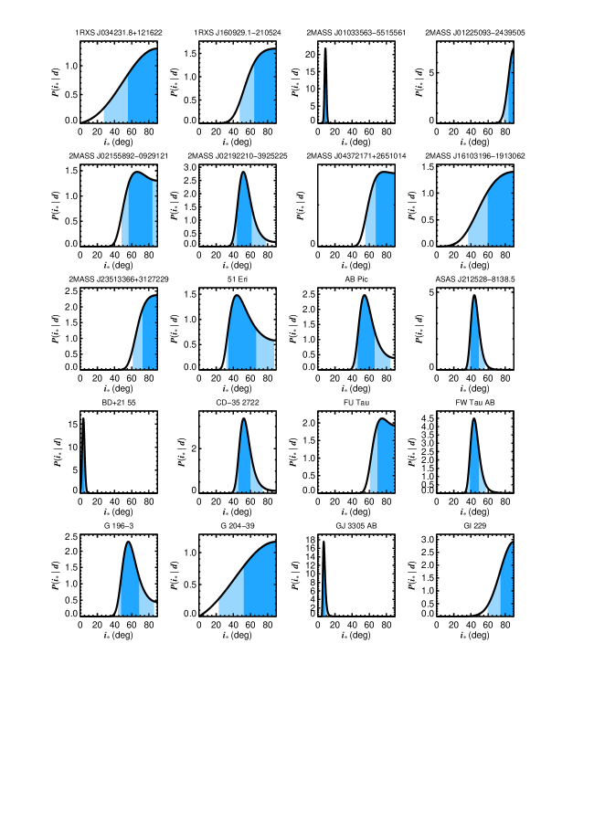
Figure 6: Posterior distributions for line-of-sight stellar inclinations determined in this study. Blue shaded regions show 1-$\sigma$ and 2-$\sigma$ credible intervals. Stars viewed equator-on have inclinations of 90$\arcdeg$, while pole-on orientations have inclinations of 0$\arcdeg$. Note that the direction of the angular momentum vector in the sky plane is usually unknown, as is its orientation toward or away from the observer. For comparison, an isotropic prior distribution is shown in Figure 8.

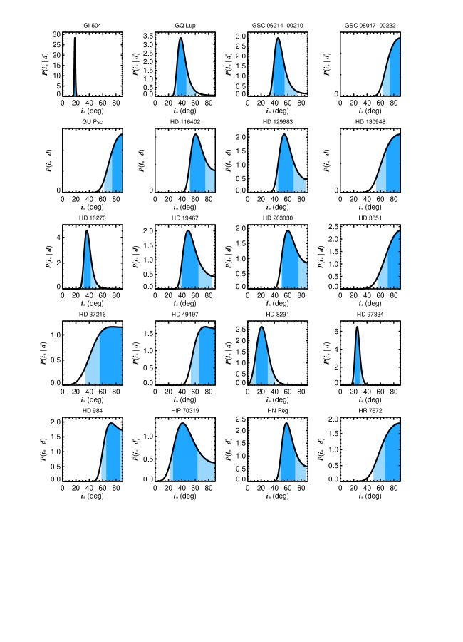
Figure 7: Posterior distributions for line-of sight stellar inclinations. See Figure 6 for details. For comparison, an isotropic prior distribution is shown in Figure 8.

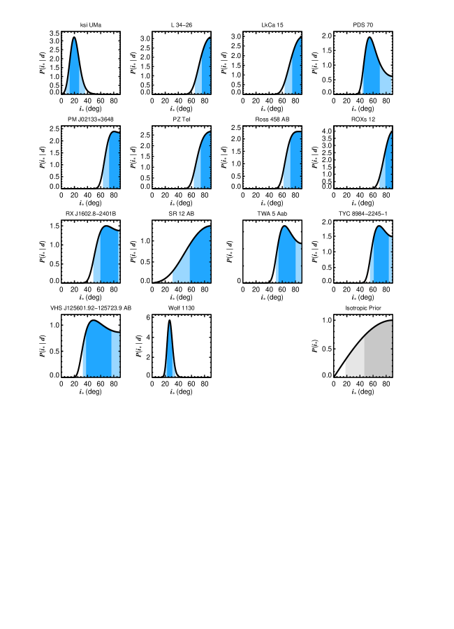
Figure 8: Posterior distributions for line-of sight stellar inclinations. See Figure 6 for details. For comparison, an isotropic prior distribution is shown in the bottom right panel.

4.5 Stellar Inclinations

Our approach to constrain $i_{*}$ relies on the Bayesian probabilistic framework developed by Masuda & Winn (2020), which takes into account the correlation between the projected and equatorial rotational velocities $v\sin i_{*}$ and $v_{\mathrm{eq}}$. Assuming normally distributed measurement errors for $v\sin{i_{*}}$, $P_{\mathrm{rot}}$, and $R_{*}$; sufficiently precise measurements of the rotation period (at the $\lesssim$20% level); and uniform priors for all three parameters, we show in Appendix A that the posterior distribution of $i_{*}$ can be expressed as:

$${}P(i_{*}\mid P_{\mathrm{rot}},R_{*},v\sin i_{*})\propto\sin i_{*}\times\frac{e^{-\frac{\big{(}v\sin i_{*}-\frac{2\pi R_{*}}{P_{\mathrm{rot}}}\sin i_{*}\big{)}^{2}}{2\big{(}\sigma_{v\sin i_{*}}^{2}+\sigma_{v_{\mathrm{eq}}}^{2}\sin^{2}i_{*}\big{)}}}}{\sqrt{\sigma_{v\sin i_{*}}^{2}+\sigma_{v_{\mathrm{eq}}}^{2}\sin^{2}i_{*}}},$$ (9)

where

$${}\sigma_{v_{\mathrm{eq}}}=\frac{2\pi R_{*}}{P_{\mathrm{rot}}}\sqrt{\Big{(}\frac{\sigma_{R_{*}}}{R_{*}}\Big{)}^{2}+\Big{(}\frac{\sigma_{P_{\mathrm{rot}}}}{P_{\mathrm{rot}}}\Big{)}^{2}}.$$ (10)

The resulting line-of-sight inclination posteriors for all 53 host stars are shown in Figures 6–8, and summary statistics are listed in Table 4.1. Constraints on the stellar inclination vary dramatically from star to star depending on the precision of the input rotation period, projected rotational velocity, and stellar radius. In some cases when these constraints are poor, the data add very little information and the posterior on $i_{*}$ resembles that for an isotropic prior, $\sin i_{*}$. Most inclination uncertainties span $\approx$10$\arcdeg$–40$\arcdeg$, but in some cases the posterior is very well constrained to within 1–2 degrees. As expected from random orientations, the majority of inclination angles peak at high values of $i_{*}$ $>45\arcdeg$, with many consistent with equator-on orientations of $i_{*}=90\arcdeg$. BD+21 55 has the most pole-on orientation with $i_{*}=3.8^{+1.2}_{-1.6}\arcdeg$.

For cases where the host star is a binary, it is assumed that the measurements of $P_{\mathrm{rot}}$ and $v\sin i_{*}$ are for the brighter component, and therefore that the inclination usually reflects the more massive member of the system. In these cases, and especially when the mass ratio is near unity, these constraints should be treated with caution because it is possible that the companion could impact the input values of period, radius, or projected rotational velocity.

The inferred equatorial velocity should always be higher than the projected rotational velocity for any line-of-sight inclinations that depart from 90$\arcdeg$. In several instances in Table 3.3, the $v\sin i_{*}$ value is larger than $v_{\mathrm{eq}}$, but for most of these systems they are consistent to within 1–2 $\sigma$. However, there are a few notable exceptions including 2MASS J01225093–2439505 ($v_{\mathrm{eq}}$ = 12.4 $\pm$ 1.0 km s^-1; $v\sin i_{*}$ = 18.1 $\pm$ 0.5 km s^-1) and Gl 229 ($v_{\mathrm{eq}}$ = 1.0 $\pm$ 0.2 km s^-1; $v\sin i_{*}$ = 2.8 $\pm$ 0.4 km s^-1). This discrepancy may be due to overestimated rotational broadening measurements, underestimated radius estimates, or periods that are overestimated. Longer-than-expected rotation periods could originate from stars with solar-like dynamos that have both strong differential rotation and spots located at non-equatorial latitudes such that the observed modulations are not tracking equatorial rotation regions. 2MASS J01225093–2439505 and Gl 229 are individually discussed in more detail in Appendix B. For this work, we treat the posterior distributions of $i_{*}$ at face value when $v_{\mathrm{eq}}<v\sin i_{*}$ because, when this occurs, the Bayesian framework we make use of yields qualitatively similar results to $v_{\mathrm{eq}}=v\sin i_{*}$; both imply an equator-on orientation with a posterior “pressed up” against $i_{*}=90\arcdeg$.

4.6 Orbital Inclinations

Probability distributions for orbital inclinations are assembled from the literature for companions with orbit fits to various combinations of relative astrometry, absolute astrometry, and radial velocities. This limits the available sample of obliquity constraints to 21 companions at separations where orbital motion is apparent on timescales of years to a few decades. For our sample the range of separations spans 10–250 AU, with most companions residing between 10–100 AU.

When possible, actual orbital inclination posterior distributions are used in our analysis, but in some instances we make use of our own approximations (for example, assumptions of normality) based on the reported summary statistics such as the mean and standard deviation. Orbital inclination posteriors for eight systems are taken from the uniform analysis in Bowler et al. (2020a), which makes use of the orbitize! orbit-fitting package (Blunt et al. 2017; Blunt et al. 2020): 1RXS J034231.8+121622 B, 2MASS J23513366+3127229 B, CD-35 2722 B, Gl 504 B, HD 49197 B, $\kappa$ And B, PZ Tel B, and TWA 5 B. The orbits of two other companions were separately fit using the same package and are directly adopted for this study: 2M0122–2439 b (Bryan et al. 2020b) and ROXs 12 B (Bryan et al. 2016). Eight systems have reported posteriors that are approximately normal, so we adopt Gaussian distributions for the following: 51 Eri b (Dupuy et al. 2022a), AB Pic b (Palma-Bifani et al. 2022), Gl 229 B (Feng et al. 2022), HD 984 B (Franson et al. 2022a), HD 19467 B (Maire et al. 2020), HD 130948 BC (Wang et al. in prep; T. Dupuy, 2022, priv. communication), HD 7672 B (Brandt et al. 2019), PDS 70 b (Wang et al. 2020), and VHS J125601.92-125723.9 b (Dupuy et al. 2022b). Finally, for two systems the inclination distributions are digitally extracted: GQ Lup B (Stolker et al. 2021) and GSC 6214-210 B (Pearce et al. 2019). The distribution medians and 68.3% credible intervals are summarized in Table 4.1.

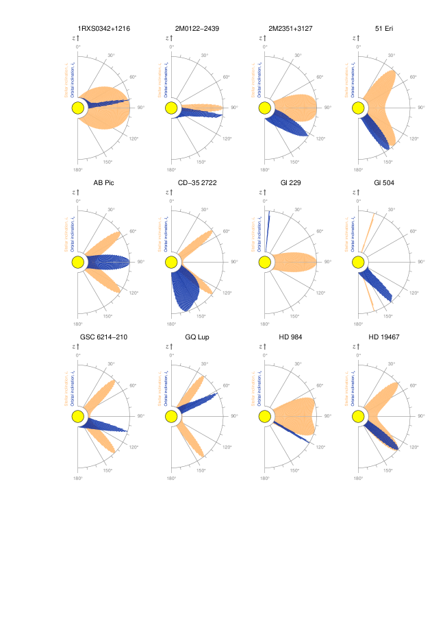
Figure 9: Line-of-sight stellar inclinations ($i_{*}$, orange) compared with the orbital inclinations of substellar companions ($i_{o}$, blue). In these “boomerang diagrams”, stellar inclinations are mirrored about the $x-y$ sky plane ($i=90\arcdeg$) because angular momentum vectors may point toward or away from the observer looking down along the $z$-axis (as depicted in the bottom right panel of Figure 10). If $i_{o}$ agrees with $i_{*}$ (e.g., HD 49197), this implies that the host and companion are consistent with spin-orbit alignment; however, the true spin-orbit angle may nevertheless be non-zero in these cases. If $i_{o}$ and $i_{*}$ disagree (e.g., Gl 504), the system is misaligned by at least the difference in the inclination angles. See Sections 2 and 4.7 for details.

Figure 10: Line-of-sight stellar inclinations ($i_{*}$, orange) compared with the orbital inclinations of substellar companions ($i_{o}$, blue). See Figure 9 caption for details. The bottom right panel depicts the orientation of the $z$ axis, pointing toward the observer, and the $x-y$ sky plane.

4.7 Minimum Stellar Obliquities

Figures 9 and 10 show the posterior distributions of $i_{*}$ and $i_{o}$ visualized in polar coordinates. Here the observer is looking down along the $z$-axis and the $x$-$y$ sky plane is located at an inclination of 90$\arcdeg$. Because the orientations of stellar inclinations in the sky plane are unconstrained, as are the senses of their spin directions (clockwise or counterclockwise from the observer’s perspective), the stellar rotational angular momentum vectors may point toward the observer or away into the plane of the sky. When assessing spin-orbit alignment—mutual agreement of orbital and angular angular momentum vectors—the stellar inclination distribution is therefore mirrored about $i=90\arcdeg$. In these polar plots the results often look like boomerang throwing sticks, so we refer to these figures as “boomerang diagrams.”

The consistency between $i_{*}$ and $i_{o}$ is quantified by sampling from these distributions and evaluating whether their absolute difference, $\Delta i$, deviates from 0$\arcdeg$. A $\Delta i$ value of 0$\arcdeg$ is consistent with alignment, $0\arcdeg<\Delta i<90\arcdeg$ is consistent with a prograde orbit, $\Delta i$ = 90$\arcdeg$ is consistent with a polar orbit, and $90\arcdeg<\Delta i$ $\leq$ $180\arcdeg$ is consistent with a retrograde orbit. However, in all cases true obliquity angles ($\psi$) can be larger. The resulting distributions of $\Delta i$ for all 21 systems are sorted by their median values in Figure 11. These differenced distributions take on a range of shapes: some are pressed up against $i=0\arcdeg$; some are bimodal, a reflection of the degeneracy of stellar inclination about the sky plane; and others significantly depart from alignment. Many distributions are quite broad and could be consistent with alignment, polar orbits, or retrograde motion. Table 4.1 summarizes the $\Delta i$ maximum a posteriori (MAP) values, median values, and credible intervals.

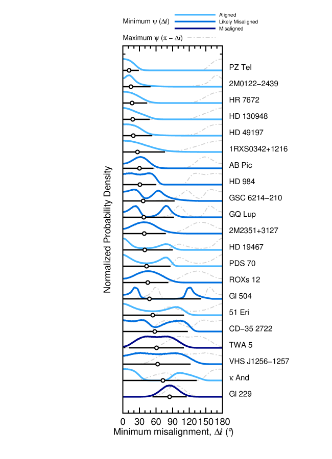
Figure 11: Distribution functions of the minimum misalignment value, $\Delta i$, equal to the absolute difference between the stellar and orbital inclinations. Median values and 95.4% credible intervals are plotted as open circles and dark blue horizontal lines. Light blue distributions are formally consistent with alignment. TWA 5 and Gl 229 are significantly misaligned (dark blue), and nine other systems are likely misaligned (blue). See Section 4.7 and Table 4.1 for details. The maximum misalignment ($\pi-\Delta i$) is shown in light gray. For Gl 229, this implies it is on a near-polar orbit.

We define two criteria to classify a system as being misaligned based on these $\Delta i$ distributions. Most of the distribution power must be located at values of $\Delta i$ away from 0$\arcdeg$. But this alone would not be a sufficient metric because a flat distribution from 0–180$\arcdeg$, for instance, could satisfy this criterion but $\Delta i$ would be unconstrained. So we also require that the MAP value is non-zero and beyond a given threshold. The characteristic uncertainty in stellar inclination measurements is about 10$\arcdeg$, so we adopt this as a reasonable value to distinguish alignment from misalignment. Systems for which $P(\Delta i>10\arcdeg)$ $\geq$ 95% and where $\Delta i$ MAP values are beyond 10$\arcdeg$ are deemed “misaligned.” Those with $P(\Delta i>10\arcdeg)$ $\geq$ 80% and $\Delta i$ MAP $>$ 10$\arcdeg$ are labeled as “likely misaligned”; most of their posterior power lay beyond that threshold. If neither are satisfied, the system is considered to be consistent with alignment. Finally, in addition to the minimum true obliquity distributions, we also overplot $\pi-\Delta i$, the maximum values of $\psi$, in Figure 11. In most cases these maximum values are near 180$\arcdeg$, showing the broad range of potential angular momentum orientations in each system.

Two companions in the sample are on significantly misaligned orbits. The orbital plane of TWA 5 B is offset with respect to the rotation axis of at least one component of the host binary TWA 5 Aab by at least 61 $\pm$ 30$\arcdeg$. The 95.4% credible interval of $\Delta i$ spans 11–110$\arcdeg$. As with most systems, this implies that prograde, polar, and retrograde orbits are allowed. Note, however, that because TWA 5 Aab is a near-equal mass resolved binary (Macintosh et al. 2001), it is possible that the stellar inclination could be impacted by the blended light curve and unresolved $v\sin i_{*}$ measurement.

Gl 229 B orbits its host in a nearly face-on orientation ($i_{o}=5.50\pm 0.16\arcdeg$; Feng et al. 2022), while we find the star is viewed nearly equator-on. The resulting minimum misalignment value is $\Delta i$ = 85${}^{+15}_{-16}\arcdeg$. Although the direction of the stellar rotation is not known, this does not impact the interpretation of the spin-orbit misalignment because in either scenario (whether it rotates clockwise or counterclockwise from the observer’s perspective), the inclination is confined close to the sky plane. As a result, the maximum value of $\psi$ ($\pi-\Delta i$) is close to the minimum value, so $\psi\approx 90\arcdeg$. Gl 229 B therefore appears to be on a polar orbit around Gl 229 A. This is the only system with this type of potentially well-constrained geometry in the sample.

We caution that this interpretation for the Gl 229 system is especially sensitive to the $v\sin i_{*}$ value of Gl 229 A because its equatorial velocity is so small (1.0 $\pm$ 0.2 km s^-1). It is difficult to reliably determine projected rotational velocities below about 2 km s^-1, so if the true $v\sin i_{*}$ value is, for instance, 0.5 km s^-1, that would be challenging to measure. Our adopted $v\sin i_{*}$ value is elevated above $v_{\mathrm{eq}}$, indicating that the projected rotational velocity may be overestimated—likely because it is near the systematics-dominated floor for broadening measurements. See Section B for a detailed discussion of this system. Additional in-depth rotational broadening analysis would help to clarify the inclination and spin-axis orientation of this system. For the purposes of this study we rely on these available measurements at face value, so a pole-on orbital orientation appears to be the most likely angular momentum architecture for this system, although this could change if the actual $v\sin i_{*}$ value of the host star is less than $\approx$1 km s^-1.

Nine companions are classified as being likely misaligned with the spin axes of their host stars: 2MASS J23513366+3127229 B, AB Pic b, CD–35 2722 B, Gl 504 B, GSC 6214-210 B, GQ Lup B, HD 984 B, ROXs 12 B, and VHS J125601.92–125723.9 b. There are a variety of reasons these systems are less confidently misaligned than for TWA 5 B and Gl 229 B. The primary contributing factors are the precision of the $v\sin i_{*}$ measurement, which impacts the width or the stellar inclination posterior, and the constraint on the orbital inclination. Improvements to both of these parameters will help narrow the resulting $\Delta i$ distributions to more definitively establish the angular momentum geometry.

Altogether, this implies that a total of 11 out of 21 systems (52${}^{+10}_{-11}$% of the sample) show signatures of offsets between the rotational and orbital angular momentum vectors. Note that this measurement assumes that host star inclinations are equally likely to point toward or away from the observer (creating the boomerang structures in Figures 9–10). If mutual alignment is a priori expected (from particular disk-based formation channels, for instance), and this non-uniform prior probability were to be imposed on the stellar inclination distributions so as to make them asymmetric about 90$\arcdeg$, this would impact the resulting $\Delta i$ distributions and the implied misalignment fraction. As expected with Bayesian probabilistic inference, the answer and interpretation will depend to some degree on the priors. We simply emphasize here that the priors for the orientation of the rotational angular momentum vectors are identical and are not conditioned on whether the orbital inclination distribution points toward or away from the observer. We discuss the implications of this prevalence of misalignments in Section 5.

The remaining ten systems are consistent with alignment: 1RXS J034231.8+121622, 2MASS J01225093–2439505, 51 Eri, HD 130948, HD 19467, HD 49197, HR 7672, $\kappa$ And, PDS 70, and PZ Tel. However, as is evident in Figure 11, the complementary distribution to $\Delta i$ for the maximum value of $\psi$ implies that there are a wide range of potential true obliquities each system can have. It is challenging to interpret individual systems with $\Delta i$ distributions consistent with 0$\arcdeg$ because these represent minimum misalignments; their true obliquities can be much larger. In many cases obliquities spanning any value from 0–180$\arcdeg$ are consistent with the observations. Instead we focus the following discussion on misaligned (and likely misaligned) systems and we develop simple population-level models to compare with our observed family of $\Delta i$ distributions.

5 Discussion

5.1 Comparison with Previous Obliquity Constraints

Several previous studies have explored spin-orbit alignment for individual systems with imaged substellar companions similar to the method we employ here:

• Bowler et al. (2017) found that the orbit of ROXs 12 B is likely to be misaligned with the spin axis of its host star, with $P(\Delta i>10\arcdeg)$ = 0.94. This is similar to the misalignment probability of 0.95 derived in this study.

• Bonnefoy et al. (2018) carried out the same analysis for Gl 504 and note possible signs of misalignment, with $P(\Delta i>10\arcdeg)$ = 0.78. We infer a higher probability of 0.91, most likely because of the more precise $v\sin i_{*}$ we adopt as well as the updated orbit constraint.

• Maire et al. (2020) found that the brown dwarf companion HD 19467 B is consistent with alignment. We reach a similar conclusion, with $P(\Delta i>10\arcdeg)$ = 0.75, which is below the threshold of 80% that we adopt for classifying systems as being “likely misaligned.”

• Bryan et al. (2020b) performed a detailed analysis of spin-orbit and spin-spin alignments in the 2MASS J01225093–2439505 system. Their results support a low stellar obliquity for the host star, consistent with our findings here.

• Schwarz et al. (2016), Wu et al. (2017), and Stolker et al. (2021) analyzed the orbital configuration of GQ Lup B with respect to the host star’s spin axis, the companion’s spin axis, and the orientation of the circumstellar disk. Although the orbit is not yet well constrained, both studies conclude that non-zero stellar obliquity is possible. We find that spin-orbit misalignment is likely in the GQ Lup system, with $P(\Delta i>10\arcdeg)$ = 0.896.

Altogether our results from this study are in good agreement with previous work focused on individual systems.

5.2 Implications of Misalignments

Most of our sample is comprised of brown dwarf companions (Figure 12), but there are two stars hosting giant planets (PDS 70 and 51 Eri) as well as a handful of objects whose masses and origin are more ambiguous (such as VHS J1256–1257 b, 2M0122–2439 b, AB Pic b, Gl 504 B, and GSC 6214-210 B). Because the overall sample size is modest, and individual constraints are fairly broad, we consider our sample as belonging to one substellar population of (predominantly) brown dwarf companions for this analysis and discussion about formation channels.

Brown dwarf companions are expected to form like stellar binaries from the turbulent fragmentation of molecular cloud cores or through disk fragmentation (e.g., Low & Lynden-Bell 1976; Bate et al. 2002; Bate 2009; Stamatellos & Whitworth 2009; Jumper & Fisher 2013). In principle, these formation sites—in cores, filamentary structures, or in disks—can result in similar orbital and rotational axes for the host and companion through a localized conservation of angular momentum during collapse. However, a variety of mechanisms have been proposed that can disrupt this alignment during or after the star formation process. This includes non-axisymmetric collapse from variable accretion, interactions with nearby protostars, or inhomogeneities in the parent cloud core (e.g., Tremaine 1991; Bate et al. 2010; Fielding et al. 2015; Offner et al. 2016); interactions with the protoplanetary disk (e.g., Lai et al. 2011; Batygin & Adams 2013; Epstein-Martin et al. 2022); or dynamical encounters with companions or passing stars at older ages (Batygin 2012; Anderson et al. 2017). There have been few large-scale empirical tests of these various models owing to the difficulty in determining obliquities for stars hosting long-period brown dwarf companions.

Observationally, close stellar binaries have been shown to be well aligned in many individual instances (e.g., Sybilski et al. 2018), although there are several notable examples of spin-orbit misalignments (e.g., Albrecht et al. 2009). Ensemble obliquity measurements of binary systems have yielded tentative or inconclusive results (Hale 1994; Justesen & Albrecht 2020). Recently, however, Marcussen & Albrecht (2022) found that most close binaries in their sample of 43 systems are consistent with alignment.

The most significant statistical result from this analysis is that spin-orbit misalignments appear to be common among stars hosting wide substellar companions. The (minimum) fraction of systems likely to be misaligned, 52${}^{+10}_{-11}$%, is higher than for cool stars hosting hot Jupiters ($\sim$5%: Winn et al. 2010; Albrecht et al. 2022) and close-in small planets (Campante et al. 2016; Winn et al. 2017). It also appears to be higher than the misalignment fraction for stars hosting debris disks ($\lesssim$10%: Le Bouquin et al. 2009; Watson et al. 2011; Greaves et al. 2014), a comparison that may be more relevant because the spatial scales of tens to hundreds of AU are closer to the population of companions considered in this study. Since debris disks are expected to trace the sites of planetesimals and planet formation, this disagreement between the incidence of misaligned debris disks and misaligned brown dwarf companions may indicate that companions in our sample did not predominantly form in disks; if this were the case, the alignment frequencies would be expected to be similar. Less is known about the overall coplanarity of systems that contain both spatially resolved debris disks and substellar companions. HD 2562 B (Konopacky et al. 2016; Maire et al. 2018) and HD 206893 B (Milli et al. 2017; Delorme et al. 2017; Marino et al. 2020; Ward-Duong et al. 2021) are notable examples of brown dwarf companions that appear to be aligned with their exterior debris disks—suggesting a disk-based origin for these companions—whereas planets orbiting HR 8799, $\beta$ Pic, and HD 106906 show a range of orientations with respect to exterior and interior disks (e.g., Dawson et al. 2011; Bailey et al. 2014; Wilner et al. 2018; Nguyen et al. 2021). A larger sample would help clarify the prevalence of aligned and misaligned orientations.

An alternative explanation is that subsequent post-formation scattering with a second object in the system (so as to alter the initial obliquity distribution) may be more common for stars hosting wide substellar companions, perhaps because multiple massive objects formed in the same disk. With a few exceptions (Haffert et al. 2019; Lagrange et al. 2019; Bohn et al. 2020b; Hinkley et al. 2022), however, most follow-up searches have not identified additional giant planets and brown dwarfs which could represent potential scatterers (e.g., Bryan et al. 2016).

It is also possible that some widely separated substellar companions could have been captured at an early age while still embedded in a dense cluster. Close encounters with passing stars can liberate planets and brown dwarfs (e.g, Parker & Quanz 2012; Daffern-Powell et al. 2022); these free-floating planets, and other isolated brown dwarfs formed during the star formation process, could then become captured onto very wide orbits by other stars, especially during the cluster dispersal phase (e.g., Perets & Kouwenhoven 2012; Parker & Daffern-Powell 2022). Without any significant realignment mechanism at these large orbital distances, the stellar obliquity distribution in such cases would be expected to be isotropic. The misaligned systems in our sample are therefore also consistent with this capture process.

There is no simple interpretation of this high misalignment fraction. If circumstellar disks are predominantly aligned with the spin axes of their host stars, this result points to a diversity of formation channels or dynamical processing in some systems. Alternatively, the observed distribution of spin-orbit orientations could reflect the primordial distribution of aligned and misaligned disks. Systems with spin-orbit misalignment are also consistent with the early capture of free-floating giant planets and brown dwarfs in dense clusters. A better understanding of the initial conditions for disks around cool stars would provide additional context to interpret results from this study.

5.3 Stellar Obliquities in Systems with Directly Imaged Planets

Alignment rates are less clear among systems with directly imaged planets, largely because long-period giant planets tend to reside around early-type stars whose rotation rates cannot be accurately determined through photometric monitoring in the same way as can be inferred for cool stars (Sepulveda et al. 2022). However, in some cases stellar inclinations and true three-dimensional orientations can be constrained using asteroseismology or spatially resolved interferometry. Below we summarize orbital and rotational angular momentum alignment in five planetary systems with previous obliquity constraints: $\beta$ Pic, HR 8799, 51 Eri, HD 206893, and PDS 70. Note that among these, only 51 Eri and PDS 70 are in our sample of 21 stars with obliquity constraints; the rest have had previous spin-orbit measurements obtained using a variety of alternative techniques.

Kraus et al. (2020) analyzed the spatial displacement of the A6 host star $\beta$ Pic in the Br$\gamma$ absorption line using VLTI/GRAVITY spectro-interferometry. When combined with the asteroseismic stellar inclination from Zwintz et al. (2019), they found that $\beta$ Pic is well aligned (to within $\leq$3 $\pm$ 5$\arcdeg$) with the orbit of $\beta$ Pic b and the outer debris disk. More recently, a second giant planet in the system, $\beta$ Pic c (Lagrange et al. 2019), was directly imaged and shown to be consistent with this coplanar geometry (Nowak et al. 2020; Lagrange et al. 2020; Brandt et al. 2021a; Lacour et al. 2021).

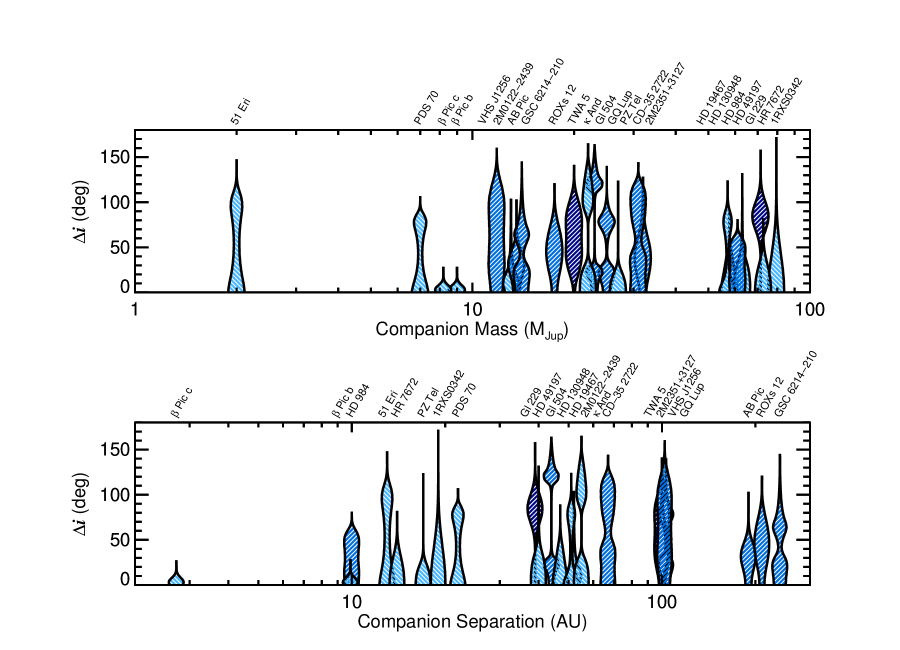
Figure 12: Top: Minimum stellar obliquity ($\Delta i$) as a function of companion mass. Color coding for each violin plot follows the scheme in Figure 11: light blue is consistent with alignment, while blue and dark blue colors denote likely spin-orbit misalignment. All planets below 10 $M_{\mathrm{Jup}}$ with stellar obliquity constraints are consistent with spin-orbit alignment, although the sample remains small. The brown dwarf companions show a mix of aligned and misaligned systems with no apparent trend with companion mass. $\beta$ Pic b and c have been added based on their true stellar obliquity from Kraus et al. (2020) and dynamical masses from Nowak et al. (2020). Note that, in general, the uncertainties in model-inferred masses (which apply to most systems in this figure) can be very large and typically range from a few $M_{\mathrm{Jup}}$ to tens of $M_{\mathrm{Jup}}$. Bottom: Same as the upper panel but for orbital separation. With the exception of HD 984 B, which is likely (though not definitively) misaligned, all companions within 20 AU are consistent with spin-orbit alignment.

The orbital inclinations (and longitudes of ascending node) of the four planets orbiting HR 8799 (Marois et al. 2008; Marois et al. 2010) have progressively improved over time with continued orbit monitoring. The precision of the constraint depends on assumptions about resonant orbits, stability, and coplanarity, but in the unconstrained case the four orbital planes lie between about 20–40$\arcdeg$ (e.g., Wang et al. 2018; Sepulveda & Bowler 2022); in the most restricted case, Zurlo et al. (2022) found an inclination of 26.9${}^{+0.16}_{-0.17}\arcdeg$ for the planetary system. Wright et al. (2011) measured an inclination of $\gtrsim$40$\arcdeg$ for the host star using oscillation frequencies from high-cadence radial velocities, which would imply a spin-orbit misalignment by at least 10$\arcdeg$. However, Sodor et al. (2014) concluded that asteroseismic analysis of HR 8799 as an A5/F0 $\gamma$ Dor variable is challenging because of resonances and amplitude variations among the pulsation frequencies. The inclination and obliquity of HR 8799 are therefore not yet reliably established, although an estimate of the core rotation period by Sepulveda et al. (2023) implies a stellar inclination in good agreement with the orbits of its four planets. Furthermore, the exterior cold disk in this system appears to be coplanar with the planets’ orbits (e.g., Faramaz et al. 2021).

Maire et al. (2019) derived a stellar inclination of the young F0 planet host 51 Eri (Macintosh et al. 2015) using the equatorial and projected rotational velocity method. The equatorial velocity was based on a rotation period of 0.65 $\pm$ 0.03 d computed using Hipparcos photometry. They conclude that the stellar inclination (39–51$\arcdeg$ or 129–141$\arcdeg$) and orbital inclination of 51 Eri b (126–147$\arcdeg$) are consistent with orbital and rotational alignment. However, Sepulveda et al. (2022) recently analyzed the TESS light curve of 51 Eri and identify it as a $\gamma$ Dor pulsating star. The variability previously attributed to rotational modulation is more likely caused by pulsation modes. Although the surface rotation rate is not constrained, the authors estimate a core rotation period of 0.9${}^{+0.3}_{-0.1}$ d and use this to deduce a stellar inclination of $\sim$62$\arcdeg$. We make use of this core rotation period estimate here; based on our stellar inclination of 54${}^{+13}_{-19}\arcdeg$ we conclude there is no evidence of misalignment.

HD 206893 hosts a brown dwarf companion (Milli et al. 2017) and giant planet (Hinkley et al. 2022) on orbits consistent with being coplanar. Delorme et al. (2017) presented ground-based photometric monitoring of the F5 host star and found clear modulations with a period very close to 1 day. They interpret this signal of 0.996 $\pm$ 0.03 d as most likely originating from a rotation period. They then use the equatorial and rotational velocities to infer a stellar inclination of 30 $\pm$ 5$\arcdeg$, which (given the symmetric nature of the distribution about 90$\arcdeg$), is consistent with the orbital inclination of 146 $\pm$ 3$\arcdeg$ for HD 206893 B and 150 $\pm$ 3$\arcdeg$ for c (Hinkley et al. 2022). This is also consistent with measurements of 40 $\pm$ 3$\arcdeg$ (Marino et al. 2020) and 45 $\pm$ 4$\arcdeg$ (Nederlander et al. 2021) for the orientation of the debris disk. However, Delorme et al. (2017) note that the photometric periodicity they measured could be attributed to stellar pulsation modes if HD 206893 is a $\gamma$ Dor variable star. This is certainly possible as F5 is near the boundary of the onset of this instability strip (Kaye et al. 1999; Aerts 2021). While the $\approx$1-day rotation period is plausible, additional monitoring of this system would be valuable to more robustly establish the nature of the periodic variations. For the time being, we therefore cautiously interpret the angular momentum geometry of this system as being potentially—but not securely—aligned.

PDS 70 hosts two accreting giant planets nested inside a transition disk (Keppler et al. 2018; Haffert et al. 2019; Zhou et al. 2021). The orbits of PDS 70 b and c have been constrained to 133${}^{+4}_{-3}\arcdeg$ and 132 $\pm$ 3$\arcdeg$, respectively, assuming non-crossing orbits and near-coplanarity (Wang et al. 2021). Thanathibodee et al. (2020) measure a rotation period of 3.03 $\pm$ 0.06 d for PDS 70 from the TESS light curve and infer a stellar rotation axis of 50 $\pm$ 8$\arcdeg$ (equal to 130 $\pm$ 8$\arcdeg$)—in good agreement with the orbits. We find a similar result consistent with spin-orbit alignment: $i_{*}$ = 60${}^{+10}_{-15}\arcdeg$, $\Delta i$ = 43${}^{+24}_{-43}$, and $P(\Delta i>10\arcdeg)$ = 0.804. These orbital and rotational orientations are also in agreement with those of the transition disk (Keppler et al. 2019). The PDS 70 system therefore appears to be in a state of organized angular momentum alignment.

In summary, a variety of constraints are now available on the true obliquities or minimum misalignments for a handful of stars hosting directly imaged planets. The $\beta$ Pic system is unambiguously aligned in $\psi$. PDS 70 is consistent with spin-orbit alignment in $\Delta i$. 51 Eri and HD 206893 are potentially aligned with their companions. The stellar inclination and obliquity of HR 8799 is not reliably constrained.

In Figure 12 we compare the minimum misalignment constraint for each system as a function of companion mass and separation. $\beta$ Pic b and c are included based on their true obliquity constraint from Kraus et al. (2020) and planet properties from Nowak et al. (2020). The sample size is modest, but we note that all four of the companions in three systems with masses below 10 $M_{\mathrm{Jup}}$ are consistent with spin-orbit alignment, and, similarly, seven of the eight companions with separations less than 20 AU are consistent with alignment. At higher masses and wider separations, there is a mixture of aligned and misaligned systems with no clear correlation with increasing brown dwarf mass or orbital separation.

Altogether, this points to an emerging trend that systems with long-period giant planets have low stellar obliquities, although the small sample size of (primarily early-type) host stars with inclination measurements remains very small. This would, however, have important implications for the formation of these companions. A uniform analysis of eccentricities by Bowler et al. (2020a, see also ) revealed that imaged planets between 5–100 AU have low eccentricities, whereas brown dwarf companions have a broader range of eccentricities. If both of these trends are validated with larger samples, this would reinforce a distinction in the orbits, obliquities, and formation of these two populations: long-period planets are most consistent with a disk-based origin with minimal dynamical evolution, whereas brown dwarf companions as a population are more aligned with formation from turbulent cloud fragmentation.

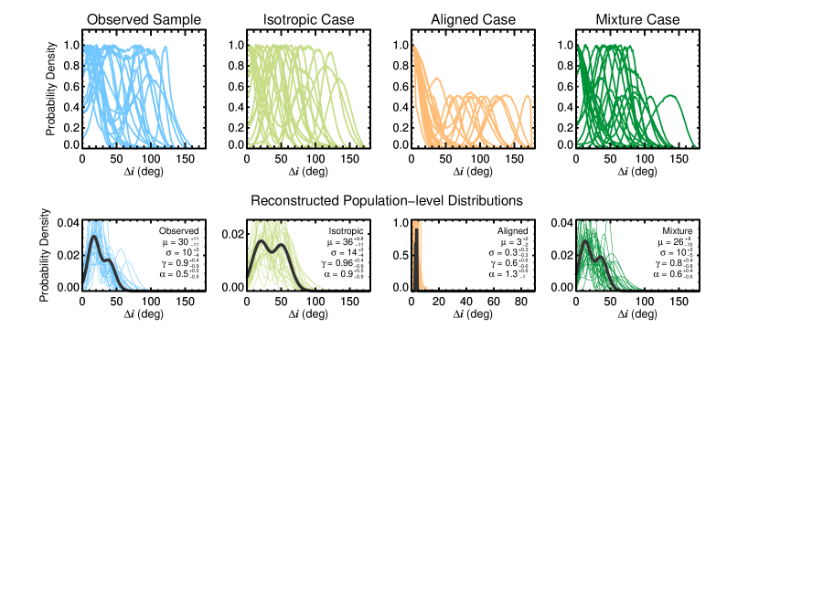
Figure 13: Top: $\Delta i$ distributions for our observed sample of substellar companions (left) compared with one synthetic realization for an isotropic stellar inclination distribution (middle left), perfect spin-orbit alignment (middle right), and a random mixture of synthetic isotropic and aligned distributions in equal proportions (right). The observed sample is qualitatively most similar to the isotropic or mixture cases, but differs substantially from a purely aligned scenario. Bottom: Reconstructed underlying distributions for each sample using hierarchical Bayesian modeling. Here the flexible LGB distribution is used for our population-level model, and constraints on hyperparameter posteriors are listed in each panel. The population-level distribution for the observed sample closely resembles a mixture of isotropic and aligned systems. The thick curve shows the LGB distribution using median hyperparameter values, while thin curves show 30 draws from the MCMC chains. Note that the scale has been adjusted in the aligned panel (middle right).

5.4 The Underlying Distribution of $\Delta i$ with Hierarchical Bayesian Modeling

Although it is difficult to make a meaningful constraint on the underlying true obliquity distribution, we can nevertheless compare our observed sample of $\Delta i$ distributions with extreme cases of isotropic stellar orientations and completely aligned spin-orbit orientations, as well as a mixture of these two scenarios. We generate three synthetic datasets for these purposes.

For the isotropic case, we randomly draw a stellar inclination from a $\sin i_{*}$ distribution from 0 to $\pi$/2. Assuming the measurement of $i_{*}$ follows a Gaussian with a standard deviation of 10$\arcdeg$, which is a characteristic level of uncertainty from this study, we then mirror the distribution across 90$\arcdeg$ to reflect the unknown orientation of the spin angular momentum vector. For each system we use the measured $i_{o}$ and our new $i_{*}$ distributions to compute a realization of a sample of $\Delta i$ distributions assuming isotropic stellar line-of-sight inclinations.

For the aligned case, the procedure is the same as the isotropic case, except instead of selecting a randomly drawn mean value of $i_{*}$ we use the MAP value of $i_{o}$. If this lies between 0 to $\pi$/2 then $i_{*}$ is mirrored onto the $\pi/2$ to $\pi$ range, and vice versa. The absolute difference then provides a distribution of minimum obliquities assuming perfect spin-orbit alignment and an unknown orientation of $\overrightarrow{L_{*}}$ to mimic the information available to an observer.

For the mixture case, we randomly draw 10 unique distributions from the isotropic sample described above and nine from the aligned sample to create an approximately even mixture of 19 systems. This represents an intermediate scenario between the two extreme examples of completely aligned and independent angular momentum architectures.

The observed and synthetic limiting cases are shown in the upper panels of Figure 13. $\Delta i$ distributions for the isotropic case are broadly located between about 0–130$\arcdeg$. As expected, the aligned case is clustered at $\Delta i$ = 0$\arcdeg$ with many individual distributions being bimodal because $i_{*}$ is often bimodal. Altogether, the observed sample better resembles the isotropic or mixed cases with many distributions peaking at non-zero $\Delta i$ values.

To quantify this agreement, we employ hierarchical Bayesian modeling to reconstruct the underlying population-level distributions of the real and synthetic samples. Our general strategy follows the framework described by Hogg et al. (2010), in which an importance sampling approximation of the likelihood function enables a phased approach to the problem: individual-level posteriors can be generated first and subsequently sampled to constrain hyperparameters of an assumed population-level model.

Here we adopt a flexible model introduced by Iriarte et al. (2021) called the Lambert generalized bimodal (LGB) distribution, which was developed to introduce skewness to the generalized bimodal distribution. The LGB distribution has four parameters: the location parameter $\mu$ (defined for all real numbers), the scale parameter $\sigma$ (defined for positive numbers), and the shape parameters $\gamma$ (defined over $[$0, 2)) and $\alpha$ (defined over (0, $e$), where $e$ is Euler’s constant). Depending on these parameters, the LGB distribution can be unimodal, bimodal, symmetric, or asymmetric; examples of the diversity of shapes can be seen in Figure 1 of Iriarte et al. (2021). $\gamma$ controls the bimodality of the distribution, and $\alpha$ determines the relative heights of the bimodal peaks or unimodal asymmetry.

This choice of the underlying model is motivated by the bimodal nature of many $\Delta i$ distributions, which tend to produce power at secondary peaks, as well as the versatility and modest number of hyperparameters of the LGB distribution. It is not, however, otherwise physically motivated, and certainly other distributions or mixture models could be used in its place to capture the behavior of the (unknown) distribution from which this sample was drawn. The exact shape and inferred parameter values are less important for this exercise than a comparison of the results from the observed sample with the isotropic, aligned, and mixture cases.

The LGB probability distribution function for $\Delta i$ takes on the following form:

$$f(\Delta i|\mu,\sigma,\gamma,\alpha)=\frac{\gamma+z^{2}}{\sigma(\gamma+1)}\phi(z)\alpha^{\Phi(z)-\frac{z}{\gamma+1}\phi(z)}$$ (11)

$$\times\Big{(}1-\ln{\alpha}\big{(}1-\Phi(z)+\frac{z}{\gamma+1}\phi(z)\big{)}\Big{)}$$

Where $z$ = $(\Delta i-\mu)/\sigma$, $\phi(z)$ is the standard normal distribution, $e^{-0.5z^{2}}/\sqrt{2\pi}$, and $\Phi(z)$ is the cumulative distribution function of the standard normal: $\big{(}1+\mathrm{erf}(z/\sqrt{2})\big{)}/2$.

Hierarchical Bayesian modeling of all three samples is carried out in a similar fashion as in Bowler et al. (2020a) for the case of the two-parameter Beta distribution, except here the posteriors of four hyperparameters are sampled. We implement a Metropolis-Hastings Markov Chain Monte Carlo (MCMC) algorithm (Metropolis et al. 1953; Hastings 1970) with tunable Gaussian jump parameters and Gibbs sampling. Uniform hyperpriors are adopted for all four hyperparameters: $\mathcal{P}(\mu)$ $\sim$ $\mathcal{U}(-1000\arcdeg,1000\arcdeg)$, so as to allow the location parameter to drift beyond the range of the data, $\mathcal{P}(\sigma)$ $\sim$ $\mathcal{U}(0\arcdeg,1000\arcdeg)$, $\mathcal{P}(\gamma)$ $\sim$ $\mathcal{U}(0,2)$, and $\mathcal{P}(\alpha)$ $\sim$ $\mathcal{U}(0,e)$.. A single Markov chain ran for 10⁵ steps with parameter acceptance rates generally falling between 20–50%. Trace plots are visually analyzed to assess convergence, and a burn-in fraction of 30% is adopted.

Results are shown in the bottom panels of Figure 13. The family of hyperparameter posterior distributions is clustered between $\Delta i$ values of $\approx$0–50$\arcdeg$ for the observed sample ($\mu=30^{+11}_{-11}$, $\sigma=10^{+3}_{-4}$, $\gamma=0.9^{+0.4}_{-0.9}$, and $\alpha=0.5^{+0.3}_{-0.5}$), $\Delta i\approx$0–80$\arcdeg$ for the isotropic case ($\mu=36^{+10}_{-11}$, $\sigma=14^{+3}_{-4}$, $\gamma=1.0^{+0.4}_{-0.9}$, and $\alpha=0.9^{+0.5}_{-0.9}$), $\Delta i\lesssim$10$\arcdeg$ for the aligned case ($\mu=3^{+2}_{-2}$, $\sigma=0.3^{+0.3}_{-0.3}$, $\gamma=0.6^{+0.6}_{-0.6}$, and $\alpha=1.3^{+0.6}_{-1}$), and $\Delta i\approx$0–50$\arcdeg$ for the mixture case ($\mu=26^{+8}_{-10}$, $\sigma=10^{+3}_{-5}$, $\gamma=0.8^{+0.4}_{-0.8}$, and $\alpha=0.6^{+0.4}_{-0.6}$). Quoted values represent median and 68.3% credible intervals of the marginalized posteriors.

Following Nagpal et al. (2022), we define the metric $\mathcal{M}$ to quantify the level of agreement between the family of underlying distributions in the observed sample and the three synthetic cases:

$$\mathcal{M}=\frac{1}{N}\sum_{n=1}^{N}\int\left|f(\Delta i)_{\mathrm{obs},n}-f(\Delta i)_{\mathrm{model},n}\right|\,d\Delta i$$ (12)

$\mathcal{M}$ is the average area of the absolute difference between random posterior draws ($n$) from the underlying model of the observed sample, $f(\Delta i)_{\mathrm{obs},n}$, compared with the isotropic, aligned, or mixture models, $f(\Delta i)_{\mathrm{model},n}$. Lower values of $\mathcal{M}$ correspond to better agreement between the two underlying families of distributions. We also quantify the spread in this metric with the standard deviation of these absolute residual areas:

$$\sigma_{\mathcal{M}}=\sqrt{\frac{\sum_{n=1}^{N}\Big{(}\int\left|f(\Delta i)_{\mathrm{obs},n}-f(\Delta i)_{\mathrm{model},n}\right|\,d\Delta i-\mathcal{M}\Big{)}}{N-1}}$$ (13)

We find $\mathcal{M}$ and $\sigma_{\mathcal{M}}$ values of 0.83 $\pm$ 0.30 when comparing the observed and isotropic case, 2.00 $\pm$ 0.46 for the observed and aligned case, and 0.67 $\pm$ 0.24 for the observed and mixture case. The inferred distribution for the observed sample is in much better agreement with the mixture scenario than either the pure aligned or isotropic cases. Indeed, all four parameters in the LGB distribution model are consistent at the 1-$\sigma$ level with the mixture sample. The aligned scenario has the poorest agreement among the three simulated samples that we tested. Although we do not attempt to constrain the relative proportion of isotropic versus aligned orbits that best fit the observed sample, the good agreement with the equal mixture suggests that there are more aligned cases in our observations than would be expected for a purely isotropic distribution.

Overall, there does not appear to be a strong correlation between the orbital and rotational planes for systems with wide substellar companions. These results reinforce the view that misalignments are common among brown dwarf companions. A larger sample and more precise individual constraints will help to clarify this picture in the future.

5.5 Sample Biases

There are several observational biases that are important to highlight as they are likely to impact the sample selection from this study with varying degrees of significance. These are individually detailed below and summarized in Section 5.5.8.

5.5.1 Light Curve Selection Biases

Because our strategy to constrain $i_{*}$ relies on rotation period measurements, any biases that impact our ability to detect and interpret periodic photometric modulations will influence the types of host stars we can analyze. For instance, light curves with a limited time baseline are inherently more sensitive to brighter stars with larger-amplitude variations and shorter rotation periods. Some of the TESS light curves we rely on comprise only a single 27-day sector (see Table 3.3), which means we would only be able to reliably establish periods on timescales of about half that baseline ($\sim$13 d). The Sun has a small surface spot covering fraction, long equatorial rotation period (24.5 d), and brightness variations typically under 0.1% (Reinhold et al. 2020). Similarly old G dwarfs would not be recovered in TESS, so inclination and obliquity measurements for these types of host stars would not be possible using methods that rely on photometric rotation periods. As a result, there is very likely a selection bias in this study in favor of systems with brighter, younger, and later-type host stars in our sample, as has been recently established by Masuda (2022) for Sun-like stars in the Kepler field. This age bias is already present for systems with directly imaged planets, but it is likely reinforced for stars with brown dwarf companions as well by disfavoring older stars.

5.5.2 Pole-on Orientations

We also expect there to be a geometric bias associated with selecting stars based on the presence of light curve modulations. For stars with solar-like dynamos, spot distributions located in equatorial regions would be more visible and would produce higher amplitude variations if seen in an equator-on orientation. Pole-on viewing angles are inherently geometrically unlikely, but for Sun-like stars this dearth of pole-on viewing angles is likely to be reinforced. However, high-latitude and polar spots are commonly observed on the surfaces of rapidly rotating active stars (Strassmeier 2009; Yadav et al. 2015; Roettenbacher et al. 2016) as a result of youth, spin-orbit coupling in close binaries, or low stellar masses with large convective envelopes. If the dominant spot structure is located in a large polar cap-like spot, and the evolution of that spot is slow, the impact on brightness variations in a light curve would be small for a star viewed pole-on compared to a similar spot rotating in and out of view in equatorial regions. There may therefore be a two-fold selection bias against pole-on orientations near $i_{*}$=0$\arcdeg$ as a result of the lack of polar spot structures for Sun-like stars and long-lived polar spots for active stars in the sample.

This possible bias against pole-on systems can be directly tested with our sample. Three out of 53 stars with inclination constraints in Table 4.1 have posterior MAP values of $i_{*}$ under 10$\arcdeg$. For an isotropic inclination distribution, $P(i_{*})=\sin i_{*}$, the probability of obtaining an orientation within 10$\arcdeg$ of pole-on is $\int_{i_{*}=0\arcdeg}^{i_{*}=10\arcdeg}\sin i_{*}di_{*}$ = 0.015. The expectation value in a sample of 53 stars is 0.8, so we would expect about one star to be viewed this way. This is similar to the number of near-pole on stars in our sample. We therefore do not find strong evidence for a significant bias disfavoring pole-on orientations.

5.5.3 Differential Rotation

Differential rotation is expected to be common and has been observed in many stars. Starspots located at mid- or high-latitudes can result in a systematically longer inferred rotation period than the true equatorial rotation period. The severity of this bias is increased for spots located at higher latitudes and stars with stronger levels of shear. An overestimated rotation period will underestimate the equatorial velocity, which in turn will overestimate the stellar inclination when using projected rotational velocity to infer $i_{*}$.

For example, the active regions in the Sun are confined to latitudes of about $\pm$30$\arcdeg$ where the rotation period is $\approx$25.7 d (based on the latitude-dependent relations for differential rotation from Snodgrass & Ulrich 1990). This is only 5% higher than the equatorial rotational velocity of 24.47 d, so the effect is not particularly large for old Sun-like stars with solar-like dynamos. However, using asteroseismology of stars in the Kepler field, Benomar et al. (2018) found that some solar-type stars rotate twice as fast at their equators compared to their mid-latitudes. A broad distribution of absolute shear also appears to be present among low-mass stars, even though the overall level of differential rotation decreases with effective temperature (Barnes et al. 2005; Reinhold et al. 2013; Reinhold & Gizon 2015). Although most stars are expected to follow a solar-like differential rotation law with shorter rotation periods at the equator and longer periods at the poles, antisolar rotation (with poles rotating faster than the equator) and cylindrical rotation may also be possible (Brun et al. 2017). Altogether, there is considerable uncertainty in the detailed picture of differential rotation and the overall impact of spot distributions on light curves. While we have made conservative assumptions about the uncertainties associated with our photometric rotation periods (see Section 4.2), we did not make explicit adjustments to the period values to correct them for potential systematic overestimates.

Figure 14: Assessing biases in orbital inclinations for direct imaging surveys. The sensitivity to faint substellar companions on various orbital inclinations depends on orbital eccentricity and the ratio of the angular semi-major axis, $\alpha$, and the inner working angle (IWA), which establishes whether a companion is detected or obscured (by a circular coronagraph, for example). Imaging is more sensitive to companions with low inclinations, wider orbits (higher values of $\alpha$/IWA), and higher eccentricities. These trends are corrected for isotropic orbital viewing geometry in Figure 15.

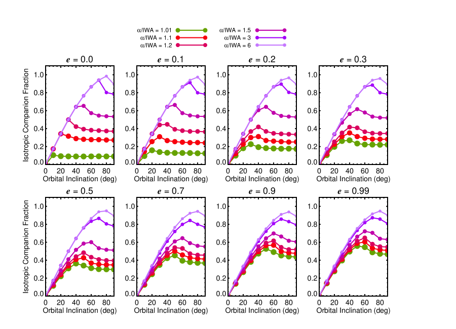
Figure 15: Same as Figure 14 but now taking into account the relative probability of observing companions with random orientations. When accounting for this $\sin i_{*}$ isotropic inclination distribution, the sensitivity to a companion is roughly constant for a given semi-major axis from the $\sin i_{*}$ envelope to $i\approx 90\arcdeg$. This results in a “truncated isotropic inclination distribution” with fewer companions having higher (more edge-on) inclinations and represents a more realistic outcome for the expected orbital inclination distribution of discoveries from blind direct imaging surveys.

One approach to assess whether there is a bias toward high inclinations is to check for an over-representation of equator-on systems in our sample in the same fashion as we did in Section 5.5.2. For this analysis, we adopt MAP values of $i_{*}$ above 80$\arcdeg$ as a threshold for equator-on viewing angles. There are 19 stars in the sample with $i_{*}>80\arcdeg$. The probability of a random orientation falling in that range is $\int_{i_{*}=80\arcdeg}^{i_{*}=90\arcdeg}\sin i_{*}di_{*}$ = 0.174, implying an expectation value of $\approx$9 for a sample of 53 stars. It does therefore appear that there are more equator-on stars than expected from chance alone. To quantify the significance of this discrepancy, we can treat this outcome as a Bernouilli trial and compute the probability of an event occurring that is at least as extreme as what was measured ($k$ = 19 out of $n$ = 53 systems) using binomial statistics. Here the probability that a success occurs is $p$ = 0.174. This statement is equivalent to computing 1 minus the probability of observing fewer than 19 stars in the 80$\arcdeg$ $<$ $i_{*}$ $<$ 90$\arcdeg$ range: $P(k\geq 19|p=0.174,n=53)$ = $1-P(k<19|p=0.174,n=53)$ = $1-\sum_{k=0}^{18}{n\choose k}p^{k}(1-p)^{n-k}$ = 0.0010. The probability of there being so many equator-on systems by chance is therefore very small. This can be interpreted either as confirmation that the overestimated rotation period bias is impacting our sample, or alternatively as a result of the Bayesian formalism we adopt, in which a broad or unconstrained $v\sin i_{*}$ value relative to $v_{\mathrm{eq}}$ will revert toward the $\sin i_{*}$ isotropic prior in which $i_{*}$ is near 90$\arcdeg$. Of course, both explanations could be at play here.

To examine whether poorly constrained $v\sin i_{*}$ values are driving the high incidence of equator-on stars, we compare the distribution of $\sigma_{v\sin i_{*}}$/$v\sin i_{*}$ values from the full sample in Table 3.3 to the subset of 19 stars with $i_{*}>80\arcdeg$. If the bias in line-of-sight stellar inclinations is caused by poor constraints on projected rotational velocities, we would expect the subsample to be shifted to higher values of $\sigma_{v\sin i_{*}}$/$v\sin i_{*}$. However, this is not what we find: the median precision of $v\sin i_{*}$ for the full sample is 3% (with a standard deviation of 13%), and for the subsample is 5% (with a standard deviation of 13%). This suggests that overestimated rotation periods, likely caused by differential rotation, are artificially increasing some of the stellar inclinations in our sample.

5.5.4 Inclination Discovery Bias

Companions found through high-contrast imaging are only visible outside of an inner working angle (IWA), which represents the closest angular separation at which a detection can be made for a given contrast. The IWA is often defined by the edge of a coronagraph or the radial extent of residual features after primary subtraction. For a star at a given distance and a companion on a circular orbit with a given semi-major axis located just outside of the IWA, a face-on orbital orientation will be more readily discoverable in a blind survey than a companion on an inclined orbit. The same companion on an edge-on orbit will spend the least time outside the IWA. This “inclination discovery bias” will impact systems with angular semi-major axes ($\alpha$) close to the IWA, or $\alpha$/IWA $\sim$ 1 (e.g., Janson 2010).

Bowler et al. (2020a) examined the impact of (the reciprocal of) this ratio to assess whether an analogous “eccentricity discovery bias” was present in their sample of companions between 5–100 AU with orbit constraints. They found that most systems at the time of discovery had $\alpha$/IWA values between 1.2–10, and therefore that this discovery bias did not play a strong role in shaping the eccentricity distribution of their sample. 13 out of 21 systems with obliquity constraints in this study overlap with the sample in Bowler et al. (2020a) that was used to analyze the impact of discovery bias. The additional systems in this study are generally at separations slightly beyond the 100 AU cutoff used in that study and generally have large $\alpha$/IWA values much greater than 1.0.

Here we examine whether an inclination discovery bias might have impacted the orbital properties of substellar companions that have been discovered in high-contrast imaging surveys (e.g., Bowler 2016; Nielsen et al. 2019; Vigan et al. 2021), which in turn could influence the minimum obliquity distribution $\Delta i$ in this study. We simulate the astrometric orbits of companions and randomly sample their projected separations on the plane of the sky as a function of orbital inclination, semi-major axis (in units of $\alpha$/IWA), and eccentricity. For each orbit we randomly draw a longitude of ascending node from 0 to 2$\pi$, argument of periastron from 0 to 2$\pi$, and time of periastron passage. The following $\alpha$/IWA values are examined: 1.01, 1.1, 1.2, 1.5, 3, and 6. 10⁵ synthetic observations of companions on unique orbits are generated for each set of sampled parameters; the proportion of observations for which the companion’s projected separation is beyond 1 $\alpha$/IWA (constituting a “detection”) represents the recovered companion fraction. Results are displayed in Figure 14.

Figure 16: Example of parameterized Bayesian priors for orbital inclinations that take into account the inclination discovery bias caused by the presence of a hard IWA in high-contrast imaging datasets (Equations 14 and 15). Note that for separations very close to the IWA, the expected orbital inclination prior deviates substantially from a traditional isotropic ($\sin i_{o}$) distribution. For circular orbits this can resemble a uniform distribution. These modified isotropic distributions are unnormalized approximations to the results in Figure 15 and depend on the angular semimajor axis $\alpha$ and orbital eccentricity. Because long-period giant planets and brown dwarf companions have distinct eccentricity distributions (Bowler et al. 2020a; Nagpal et al. 2022), a different choice for the characteristic eccentricity might be warranted depending on the properties of a newly imaged companion—for instance, $e=0.0$ for planets and $e=0.5$ for brown dwarfs.

Considering the case of circular orbits, there is a steep decline sensitivity for more inclined systems and an increase in detection sensitivity for companions on wider orbits. The recovery rate is nearly 100% for $\alpha$/IWA values beyond $\approx$3, with only the most edge-on orbits experiencing some loss in sensitivity. As soon as non-zero eccentricity is introduced, there is a general increase in sensitivity for a given $\alpha$/IWA value, except for near-face on orbits where a slight drop is evident. This behavior is readily explainable: companions on eccentric orbits will reach farther apastron distances and will spend most of their time at those locations. But for face-on circular orbits, where detection sensitivity is maximized, even a slight eccentricity will bring part of the orbit inside the IWA. This trend of overall sensitivity with increasing eccentricity persists even to unrealistically high eccentricities above 0.9. There is also a clear inclination bias present: companions on more edge-on orbits are recovered at $\approx$2–3 times lower rates compared to companions on more face-on orbits, with this drop occurring beyond inclinations of about 40$\arcdeg$ for low eccentricities and beyond 60$\arcdeg$ for high eccentricities.

However, these results do not take into account the relative geometric probability of observing face-on versus edge-on systems. To account for this effect, each curve should be adjusted by a factor of $\sin i_{*}$, as shown in Figure 15. The impact is to flatten the recovered companion fraction curves so that for any given semi-major axis, there is a roughly uniform probability of observing any orbital inclination between the $\sin i_{*}$ envelope of isotropic orbits to 90$\arcdeg$. This behavior persists to about $e$=0.5, then begins to more closely resemble an isotropic distribution at higher eccentricities, especially for large values of $\alpha$/IWA where sensitivity to companions is nearly complete. In this limit the isotropic distribution is recovered. These trends should better represent more realistic biases on the orbital inclinations of discoveries made through high-contrast imaging. The actual distribution of observed orbital inclinations will depend on the underlying range of semi-major axes, host star distances, eccentricities, and IWAs.

Figure 17: Distribution of orbital inclination MAP values for the 21 substellar companions with obliquity constraints examined in this study. Compared to an isotropic inclination distribution (gray), the observed sample has a deficit of objects with edge-on orientations between $\approx$50–90$\arcdeg$. This closely resembles predictions in Figure 15 which take into account inclination discovery bias in direct imaging surveys caused by a hard IWA.

While not the focus of this study, we note that these “truncated isotropic inclination distributions” should be more appropriate to use as Bayesian priors for the orbital plane inclinations ($\mathcal{P}(i_{o})$) of newly discovered companions located near the observational IWA than the more traditional $\mathcal{P}(i_{o})=\sin i_{o}$ inclination prior that is widely adopted for orbit fitting. Below is an approximation of these more realistic priors which account for the general behavior of inclination discovery bias as a function of semi-major axis and orbital eccentricity:

$${}\mathcal{P}(i_{o})\propto\begin{cases}\sin i_{o}&\text{if $i_{o}$ $<$ $\gamma$}\\ \sin\gamma&\text{otherwise}\end{cases}.$$ (14)

$\gamma$ is the inclination in radians beyond which the distribution is constant for increasing values of $i_{o}$. For this approximation, we implement a break from the sine curve that depends on both the angular semi-major axis $\alpha$, here parameterized as $\beta=\alpha$/IWA, and eccentricity $e$:

$${}\gamma(\beta,e)=0.5\cosh^{-1}(\beta)+1.5\log(1+e/\beta^{2}).$$ (15)

Here the inverse hyperbolic cosine term is a better fit to the $\gamma$ break values as a function of $\beta$ parameter than a polynomial. The second term is motivated by a logarithmic-like scaling of $\gamma$ with eccentricity and $\beta$. Coefficients were selected so as to reasonably agree with values in Figure 15 as a compromise between consistency with the numerical simulations and analytical simplicity. In the limit of wide orbits ($\alpha\gtrsim 11.6$ IWA), $\gamma$ $>$ $\pi/2$ and the standard isotropic distribution is recovered.

The choice of $e$ and $\beta$ may depend on the context of the system. For example, $e$=0.0 may be an appropriate choice for a new directly imaged planet, with $\beta$ corresponding to the projected separation over the IWA, whereas a moderate eccentricity of $e\approx$0.5 may be a better choice for a brown dwarf companion (Bowler et al. 2020a; Nagpal et al. 2022). Examples of these unnormalized priors are shown in Figure 16.

How do these expectations compare with actual orbital inclinations? A histogram of the median orbital inclinations from Table 4.1 is shown in Figure 17 compared to an isotropic distribution. Because the sample size is modest, we have reflected the inclination values (which span 0–180$\arcdeg$) about 90$\arcdeg$ as the predicted yields are symmetric with respect to the sky plane. The observed inclinations seems to match expectations reasonably well; there is good agreement with the isotropic case at low inclinations, and the overall distribution is approximately constant from $\approx$40–90$\arcdeg$. Altogether, this can be explained by a mixture of modest eccentricities of brown dwarfs and the range of $\alpha$/IWA values from Bowler et al. (2020a).

5.5.5 Orbital Inclination Priors

Another relevant form of inclination bias is related to the challenge of fitting orbits with small phase coverage. Most substellar companions with orbit constraints have had less than 15% of their orbits mapped with relative astrometry (Bowler et al. 2020a). This makes the inferred orbit solutions and the detailed shape of the orbital element posteriors sensitive to both random and systematic uncertainties in relative astrometry, as well as the choice of parameter priors used in the analysis. Recently, Ferrer-Chávez et al. (2021) analyzed systematic biases associated with fitting orbits to companions with very small coverage ($\approx$0.5%). They found that face-on inclinations can result in significant biases in the posterior median and mode, and that for progressively higher eccentricities, more inclined orbits can be impacted by this bias. A similar conclusion was found by O’Neil et al. (2019); without adopting their observable-based priors, inclinations are broader and less accurate. For our sample in this study, these effects can be exacerbated by the use of different approaches to orbit fitting in the literature and parameter priors that were adopted. It is therefore challenging to determine the exact scale of inclination bias caused by priors, although it is expected to be more severe for orbits with smaller fractional coverage.

5.5.6 Slow Rotation

As discussed in Section 4.7, it is challenging to reliably determine inclinations for slow rotators with equatorial velocities less than a few km s^-1 because this is near the limit where traditional spectroscopic approaches to measuring rotational broadening, macroturbulence, and microturbulence can be difficult to distinguish (e.g., Smith & Gray 1976; Gray 2005; Petigura et al. 2017; Masuda et al. 2021). The result of this is a tendency to interpret slow rotators as being equator-on, even if their actual inclinations substantially depart from 90$\arcdeg$. This may contribute to the overabundance of stellar inclinations between 80–90$\arcdeg$ discussed in Section 5.5.3. However, only seven of 53 stars with $i_{*}$ constraints have $v_{\mathrm{eq}}<3$ km s^-1, so we do not expect these systematic errors to severely impact statistical results from this study.

5.5.7 Relative Biases

In addition to overall biases that may be impacting our sample selection and inferred inclination distributions, relative biases may also be present within our sample that could in principle influence the interpretation of the misalignment results in this study. In particular, the apparent distinction between obliquities of stars hosting long-period giant planets and brown dwarf companions could instead be caused by obliquity evolution, for example through dynamical excitation over time. Imaged planets are typically young ($\lesssim$200 Myr), whereas the systems with brown dwarfs span a much broader range of ages because brown dwarfs remain bright enough to readily detect even at field ages of several Gyr. If obliquities are initially low but evolve toward a broader distribution over time, perhaps through dynamical interactions, that could manifest as a distinction between planets and brown dwarf companions as a result of their different characteristic ages. However, our sample only comprises a few field-age brown dwarfs—Gl 229, HR 7672, and HD 19467—so if obliquities are evolving then this mechanism would likely need to operate on relatively short timescales ($\lesssim$1 Gyr) corresponding to the typical age range of systems with brown dwarfs in this study.

Other possible sources of relative biases within our sample could include a dependence of obliquity on stellar host mass, metallicity, or formation environment. All of these could be explored in more detail with larger samples in the future.

5.5.8 Summary of Biases

Below we summarize the most important biases likely to impact stellar inclinations, orbital inclinations, and minimum obliquity values ($\Delta i$) in our sample.

• We expect a strong bias in favor of active stars with younger ages (faster rotation periods) and cooler temperatures (greater starspot covering fractions) as a result of the finite photometric precision and limited baseline coverage of light curves.

• Both differential rotation and slow rotation can result in a systematic overestimation of stellar inclinations. This may explain the over-representation of equator-on orientations that is present with high confidence in our larger sample of 53 host stars with inclination constraints.

• A discovery bias affecting the orbital inclination distribution is expected for companions found with high-contrast imaging. This distribution is not isotropic but instead more closely resembles a truncated $\sin i_{o}$ distribution. This deficit of edge-on orientations is reflected in the orbital inclination distribution of companions in our sample.

• Bayesian priors may be influencing the detailed shape of orbital inclination posteriors for systems with more face-on orientations and less orbital phase coverage compared to systems with well-mapped orbits.

• We do not find evidence that our sample is biased against pole-on orientations as might be expected for stars with solar-like dynamos and starspots that are confined to equatorial regions.

• Relative age biases could impact stellar obliquities for systems with giant planets and brown dwarf companions, but only if obliquity evolution occurs on relatively short timescales ($\lesssim$1 Gyr).

Altogether, it is difficult to confidently establish how these biases might be combining to affect individual and cumulative results for $\Delta i$ distributions. This certainly warrants future consideration, especially in conjunction with a better understanding of other unknown astrophysical obliquity trends that we are ignoring. These could include stellar obliquities as a function of system age, companion mass, separation, eccentricity, or multiplicity. We did not consider these in this study because the sample size and individual constraints are generally modest, but in the future these relationships can be explored in more detail with larger samples and more precise constraints on $\Delta i$.

5.6 Spin-Spin Opportunities

Most companions to the 53 host stars with stellar inclinations do not have constraints on the inclinations of their orbital planes because the physical separations in these systems are prohibitively large. However, this sample may be beneficial to explore the statistical distributions of spin-spin orientations between the host stars ($i_{*}$) and companions ($i_{p}$). A handful of obliquities have now been measured for individual brown dwarf companions and giant planets by combining rotation periods, radii, and projected rotational velocities (e.g., Bryan et al. 2020b; Bowler et al. 2020b; Zhou et al. 2020; Bryan et al. 2021; Palma-Bifani et al. 2022), but larger samples are needed to assess the prevalence of stellar-companion spin-spin alignment in order to interpret this in the context of formation secenarios (e.g., Jennings & Chiang 2021). Companions to host stars with existing inclination constraints from this study may be promising targets for follow-up photometric monitoring and high-resolution spectroscopy in the future.

6 Summary

We have carried out a homogeneous analysis of the rotation periods, inclinations, and obliquities of stars hosting directly imaged brown dwarf and giant planet companions. Below we summarize the main conclusions and interpretation from this work.

• TESS light curves for substellar host stars were uniformly examined in search of rotational modulations. Our search was isolated to spectral types $\gtrsim$F5 to avoid confusion with stellar pulsations. Supplementing these rotation periods with values from the literature yields 62 stars with period measurements, 53 of which also have $v\sin i_{*}$ values from our own new observations and previous determinations. We derived inclination posteriors using the Bayesian framework from Masuda & Winn (2020) along with general analytical expressions for inclination posteriors given $P_{\mathrm{rot}}$, $R_{*}$, and $v\sin i_{*}$ values in Appendix A.

• 21 systems with stellar inclinations also have constraints on the inclination of the companion’s orbital plane. Together these provide a measurement of $\Delta i$, the minimum value of the true spin-orbit obliquity. Companions in this subsample are predominantly brown dwarfs located between 10–100 AU with a few companions extending out to 250 AU.

• Spin-orbit misalignments for systems with substellar companions appear to be common, as revealed by $\Delta i$ distributions. Eleven of the 21 systems in our sample (52${}^{+10}_{-11}$%) have $\Delta i$ values beyond 10$\arcdeg$ with $\geq$80% confidence, indicating that misalignments are prevalent among brown dwarf companions. Depending on the orientation of the star in the sky plane and the longitude of ascending node of the orbital plane, most companions can be on prograde, polar, or retrograde orbits. This high misalignment fraction contrasts with partial or full constraints on stellar obliquities for systems with directly imaged planets, which show an emerging pattern of angular momentum alignment between the star, planet orbital plane, and, when present, the disk. We also find signs of a preference for spin-orbit alignment for companions within 20 AU. Brown dwarfs and companions at wide separations show a greater diversity of rotational and orbital angular momentum architectures.

• When the same systems are compared with stars with random orientations, stars with rotation axes aligned with orbital angular momentum vectors, and a mixture of both scenarios, our hierarchical Bayesian analysis of the underlying distributions of $\Delta i$ for the observed sample is most consistent with the even mixture and disfavors the aligned case. However, the modest sample size, generally broad $\Delta i$ distributions, potential for sample biases, and minimal information about the true obliquity angle $\psi$ limits more nuanced conclusions about how obliquities might depend on age, companion mass, and separation.

• Altogether, these results are consistent with predictions from hydrodynamic simulations that spin-orbit misalignments should be a common outcome for binary companions that form from a fragmenting molecular cloud core (e.g., Bate et al. 2010; Offner et al. 2016). Although these results could also be explained by dynamical processing of systems with primordial alignments, this would require another massive object to interact with in these systems. Large high-contrast imaging surveys have failed to uncover a population of multiple brown dwarf companions orbiting stars in non-hierarchical configurations. Some misaligned systems may also result from the capture of isolated or ejected giant planets and brown dwarfs in young dense clusters.

• We have evaluated potential biases that could be impacting the stellar and orbital inclinations in our sample. There is evidence for a higher number of systems on edge-on orbits than would be expected from chance, which may be a result of stars with differential rotation or slow rotation in the sample. More detailed modeling of the impact of these effects is warranted.

• As part of this analysis we highlight a bias in the orbital inclination distribution of companions found with high-contrast imaging in the presence of an IWA—which may be a coronagraph or residuals from primary star subtraction. This “inclination discovery bias” is most severe for objects close to the IWA and varies with semi-major axis and eccentricity. Its effect is to disfavor edge-on orientations and deviates substantially from an isotropic distribution in which $\mathcal{P}(i_{o})\propto\sin i_{o}$. The distribution of orbital inclinations for substellar companions is consistent with having been shaped by the presence of this effect. We formulate a parametric approximation for this bias, which may be useful as a more realistic Bayesian prior for orbit fits to new discoveries.

Stellar obliquities provide a rich resource to probe the formation and dynamical histories of planets and brown dwarf companions. Results from this study reinforce an emerging distinction between imaged giant planets and brown dwarf companions in terms of their orbits (Bowler et al. 2020a), demographics (Nielsen et al. 2019; Vigan et al. 2021), and mass functions (Wagner et al. 2019): brown dwarf companions are most consistent with formation in a stellar-like pathway from fragmenting turbulent clouds than within aligned disks. In the future, we expect that new discoveries from dynamically informed surveys (e.g., Franson et al. 2022b; Hinkley et al. 2022), continued astrometric orbit monitoring of known systems (e.g., Zurlo et al. 2022), precision astrometry from VLTI/GRAVITY (Nowak et al. 2020; Wang et al. 2021), and radial velocities of companions from instruments such as the Keck Planet Imager and Characterizer (Mawet et al. 2016) will be especially fruitful to build a larger sample of systems well-characterized spin-orbit constraints. In addition, spectro-interferometry capable of spatially resolving offsets from stellar rotation will enable true obliquity measurements for imaged planets orbiting early-type stars (Kraus et al. 2022). Ultimately, refined orbital inclinations and projected rotational velocities will facilitate more precise population-level obliquity constraints to carry out direct tests for differences in the obliquity distributions between long-period brown dwarf companions and directly imaged planets.

Smith (Tull Spectrograph), TESS

Appendix A Analytical Formalism to Infer Stellar Inclinations

A.1 Measurements of $v\sin i_{*}$

Masuda & Winn (2020) provide a thorough guide to infer the posterior probability distribution function of stellar inclination ($i_{*}$) given measurements or estimates of a rotation period ($P_{\mathrm{rot}}$), stellar radius ($R_{*}$), and projected rotational velocity ($v\sin i_{*}$) following a Bayesian formalism. The equatorial velocity $v_{\mathrm{eq}}$ is simply 2$\pi$$R_{*}$/$P_{\mathrm{rot}}$. If $i_{*}$, $R_{*}$, $P_{\mathrm{rot}}$, and $v\sin i_{*}$ are independent then $i_{*}$ is $\sin^{-1}(\frac{P_{\mathrm{rot}}\,v\sin i_{*}}{2\pi R_{*}})$. However, one of the important insights recognized by Masuda & Winn (2020) is that $v_{\mathrm{eq}}$ and $v\sin i_{*}$ are not independent, so accurately determining the probability distribution of $i_{*}$ must take into account the correlation between these parameters.

Under the reasonable assumption of independence between the datasets used to measure $v_{\mathrm{eq}}$ and $v\sin i_{*}$ (so that their likelihood functions are separable), and assuming $v_{\mathrm{eq}}$ and $i_{*}$ are similarly independent (so that their priors are separable), the probability distribution for $\cos i_{*}$ given a set of data $d$ is:

$$P(\cos i_{*}\mid d)\propto\mathcal{P}(\cos i_{*})\int\mathcal{L}_{v_{\mathrm{eq}}}(v_{\mathrm{eq}})\,\mathcal{L}_{v\sin i_{*}}(v_{\mathrm{eq}}\sqrt{1-\cos^{2}i_{*}})\,\mathcal{P}_{v_{\mathrm{eq}}}(v_{\mathrm{eq}})\,dv_{\mathrm{eq}}.$$ (A1)

Here $\mathcal{L}_{v_{\mathrm{eq}}}$ is the likelihood function for the equatorial velocity, $\mathcal{L}_{v\sin i_{*}}$ is the likelihood function for the projected rotational velocity, $\mathcal{P}(\cos i_{*})$ is the Bayesian prior on the cosine of the inclinations—equal to 1 for isotropic orbits—and $\mathcal{P}_{v_{\mathrm{eq}}}(v_{\mathrm{eq}})$ is the prior on the equatorial velocity. If both priors are constant then

$${}P(\cos i_{*}\mid d)\propto\int\mathcal{L}_{v_{\mathrm{eq}}}(v_{\mathrm{eq}})\,\mathcal{L}_{v\sin i_{*}}(v_{\mathrm{eq}}\sqrt{1-\cos^{2}i_{*}})\,dv_{\mathrm{eq}}.$$ (A2)

Since $v\sin i_{*}$ is typically measured from high-resolution spectroscopy, it is usually reported with Gaussian uncertainties so its likelihood function will follow a normal distribution in $v_{\mathrm{eq}}\sin i_{*}$:

$$\mathcal{L}_{v\sin i_{*}}(v_{\mathrm{eq}}\sqrt{1-\cos^{2}i_{*}})=\frac{1}{\sqrt{2\pi}\sigma_{v\sin i_{*}}}e^{-\frac{1}{2}\big{(}\frac{v_{\mathrm{eq}}\sqrt{1-\cos^{2}i_{*}}-v\sin i_{*}}{\sigma_{v\sin i_{*}}}\big{)}^{2}}.$$ (A3)

If the equatorial velocity is taken from measurements (or estimates) of $R_{*}$ and $P_{\mathrm{rot}}$ then the likelihood function for $v_{\mathrm{eq}}$ may not be straightforward to express analytically. While the stellar radius and rotation period may be normally distributed such that $R_{*}\sim\mathcal{N}(R_{*},\sigma_{R_{*}}^{2})$ and $P_{\mathrm{rot}}\sim\mathcal{N}(P_{\mathrm{rot}},\sigma_{P_{\mathrm{rot}}}^{2})$, the ratio of two independent normally distributed random variables of the form 2$\pi$$R_{*}$/$P_{\mathrm{rot}}$ itself does not generally follow a normal distribution. An analytical expression has been derived but it is not succinct, even in the case when both random variables are uncorrelated (Hinkley 1969; Oliveira et al. 2015).

However, there are certain cases when this normal ratio distribution can be approximated with a Gaussian distribution. For independent random variables $X\sim\mathcal{N}(\mu_{x},\sigma_{x}^{2})$ and $Y\sim\mathcal{N}(\mu_{y},\sigma_{y}^{2})$, Díaz-Francés & Rubio (2013) propose a second-order expansion for the variance of $Z=X/Y$ of the form $\sigma_{z}^{2}=\beta^{2}\big{(}\delta_{x}^{2}+\delta_{y}^{2}\big{)}$, where $\beta=\mu_{x}/\mu_{y}$, $\delta_{x}=\sigma_{x}/\mu_{x}$, and $\delta_{y}=\sigma_{y}/\mu_{y}$. Smaller values of $\delta_{x}$ and $\delta_{y}$ produce better agreement between the normal approximation and true distribution function. In general, the normal approximation is good if $\delta_{y}$ is small ($\lesssim$0.2). For the application to $v_{\mathrm{eq}}$ this corresponds to a rotation period measurement at the $\lesssim$20% level, which is satisfied for all targets we consider in this study.

Under these assumptions the likelihood function for $v_{\mathrm{eq}}$ becomes

$${}\mathcal{L}_{v_{\mathrm{eq}}}(v_{\mathrm{eq}})\approx\frac{1}{\sqrt{2\pi}\sigma_{v_{\mathrm{eq}}}}e^{-\frac{1}{2}\big{(}\frac{v_{\mathrm{eq}}-\frac{2\pi R_{*}}{P_{\mathrm{rot}}}}{\sigma_{v_{\mathrm{eq}}}}\big{)}^{2}},$$ (A4)

where

$${}\sigma_{v_{\mathrm{eq}}}=\frac{2\pi R_{*}}{P_{\mathrm{rot}}}\sqrt{\Big{(}\frac{\sigma_{R_{*}}}{R_{*}}\Big{)}^{2}+\Big{(}\frac{\sigma_{P_{\mathrm{rot}}}}{P_{\mathrm{rot}}}\Big{)}^{2}}$$ (A5)

Then the expression for the posterior in $\cos i$ is

$$P(\cos i_{*}\mid d)\propto\int\frac{1}{\sqrt{2\pi}\sigma_{v\sin i_{*}}}e^{-\frac{1}{2}\big{(}\frac{v_{\mathrm{eq}}\sqrt{1-\cos^{2}i_{*}}-v\sin i_{*}}{\sigma_{v\sin i_{*}}}\big{)}^{2}}\,\frac{1}{\sqrt{2\pi}\sigma_{v_{\mathrm{eq}}}}e^{-\frac{1}{2}\big{(}\frac{v_{\mathrm{eq}}-\frac{2\pi R_{*}}{P_{\mathrm{rot}}}}{\sigma_{v_{\mathrm{eq}}}}\big{)}^{2}}\,dv_{\mathrm{eq}}$$

$${}P(\cos i_{*}\mid d)\propto\frac{1}{2\pi\sigma_{v_{\mathrm{eq}}}b\sqrt{1-\cos^{2}i_{*}}}\int e^{-\frac{1}{2}\big{(}\frac{v_{\mathrm{eq}}-a}{b}\big{)}^{2}}\,e^{-\frac{1}{2}\big{(}\frac{v_{\mathrm{eq}}-c}{\sigma_{v_{\mathrm{eq}}}}\big{)}^{2}}\,dv_{\mathrm{eq}}$$ (A6)

where $a=v\sin i_{*}/\sqrt{1-\cos^{2}i_{*}}$, $b=\sigma_{v\sin i_{*}}/\sqrt{1-\cos^{2}i_{*}}$, and $c=2\pi R_{*}/P_{\mathrm{rot}}$. The integrand in Equation A6 takes the form of the product of two normal distributions, which itself is a normal distribution:

$${}\mathcal{N}(\mu_{1},\sigma_{1}^{2})\times\mathcal{N}(\mu_{2},\sigma_{2}^{2})=\frac{e^{-\frac{(\mu_{1}-\mu_{2})^{2}}{2(\sigma_{1}^{2}+\sigma_{2}^{2})}}}{\sqrt{2\pi(\sigma_{1}^{2}+\sigma_{2}^{2})}}\times\mathcal{N}(\mu_{12},\sigma_{12}^{2});$$ (A7)

here $\mu_{12}$ and $\sigma_{12}^{2}$ are the mean and variance of the resulting distribution:

$$\mu_{12}=\frac{\mu_{1}/\sigma_{1}^{2}+\mu_{2}/\sigma_{2}^{2}}{1/\sigma_{1}^{2}+1/\sigma_{2}^{2}},$$ (A8)

$$\sigma_{12}^{2}=\frac{\sigma_{1}^{2}\sigma_{2}^{2}}{\sigma_{1}^{2}+\sigma_{2}^{2}}.$$ (A9)

Making use of Equations A6 and A7, the posterior distribution for $\cos i_{*}$ can be rewritten as

$$P(\cos i_{*}\mid d)\propto\frac{1}{\sqrt{1-\cos^{2}i_{*}}}\,\frac{e^{-\frac{(a-c)^{2}}{2(b^{2}+\sigma_{v_{\mathrm{eq}}}^{2})}}}{\sqrt{2\pi(b^{2}+\sigma_{v_{\mathrm{eq}}}^{2})}}\int\mathcal{N}(\mu_{12},\sigma_{12}^{2})\,dv_{\mathrm{eq}}$$

$$P(\cos i_{*}\mid d)\propto\frac{1}{\sqrt{1-\cos^{2}i_{*}}}\,\frac{e^{-\frac{(a-c)^{2}}{2(b^{2}+\sigma_{v_{\mathrm{eq}}}^{2})}}}{\sqrt{b^{2}+\sigma_{v_{\mathrm{eq}}}^{2}}}$$ (A10)

Substituting in the values of $a$, $b$, and $c$ gives the following expression for the posterior probability of the cosine of the stellar inclination:

$${}P(\cos i_{*}\mid d)\propto\frac{e^{-\frac{\big{(}v\sin i_{*}-\frac{2\pi R_{*}}{P_{\mathrm{rot}}}\sqrt{1-\cos^{2}i_{*}}\big{)}^{2}}{2\big{(}\sigma_{v\sin i_{*}}^{2}+\sigma_{v_{\mathrm{eq}}}^{2}(1-\cos^{2}i_{*})\big{)}}}}{\sqrt{\sigma_{v\sin i_{*}}^{2}+\sigma_{v_{\mathrm{eq}}}^{2}(1-\cos^{2}i_{*})}}.$$ (A11)

The uncertainty in the equatorial velocity $v_{\mathrm{eq}}$ is given in Equation A5.

Finally, it can be useful to represent the stellar inclination constraint in terms of inclination $i_{*}$ itself. This can be achieved using a variable transformation of the form $f(i_{*})\,di_{*}=g(y)\,dy$. Here $y$ is a function of $i_{*}$, $y=y(i_{*})=\cos i_{*}$, and $g(y)$ is the posterior distribution for $\cos i_{*}$, $P(\cos i_{*}\mid d)$. Therefore $f(i_{*})=P(\cos i_{*}\mid d)\,|d\cos i_{*}/di_{*}|$ = $P(\cos i_{*}\mid d)\sin i_{*}$. The posterior of the stellar inclination in radians becomes

$${}P(i_{*}\mid d)\propto\sin i_{*}\times\frac{e^{-\frac{\big{(}v\sin i_{*}-\frac{2\pi R_{*}}{P_{\mathrm{rot}}}\sin i_{*}\big{)}^{2}}{2\big{(}\sigma_{v\sin i_{*}}^{2}+\sigma_{v_{\mathrm{eq}}}^{2}\sin^{2}i_{*}\big{)}}}}{\sqrt{\sigma_{v\sin i_{*}}^{2}+\sigma_{v_{\mathrm{eq}}}^{2}\sin^{2}i_{*}}}.$$ (A12)

Under the assumptions outlined above, Equations A11 and A12 provide the full (unnormalized) expressions for the distribution function of a stellar inclination and its cosine given measurements of $v\sin i_{*}$, $P_{\mathrm{rot}}$, and $R_{*}$.

In Figure 18 we test these relations with the same examples used in Masuda & Winn (2020). Here we assume $R_{*}$ = 1.0 $\pm$ 0.1 $R_{\odot}$ and $P_{\mathrm{rot}}$ = 5.059 $\pm$ 0.88 d, which is tailored to give $v_{\mathrm{eq}}$ = 10 $\pm$ 2 km s^-1. Compared to their Figure 1, our results are in good agreement for two cases of projected rotational velocities: $v\sin i_{*}$ = 9.8 $\pm$ 2.0 km s^-1 and $v\sin i_{*}$ = 4.0 $\pm$ 2.0 km s^-1.

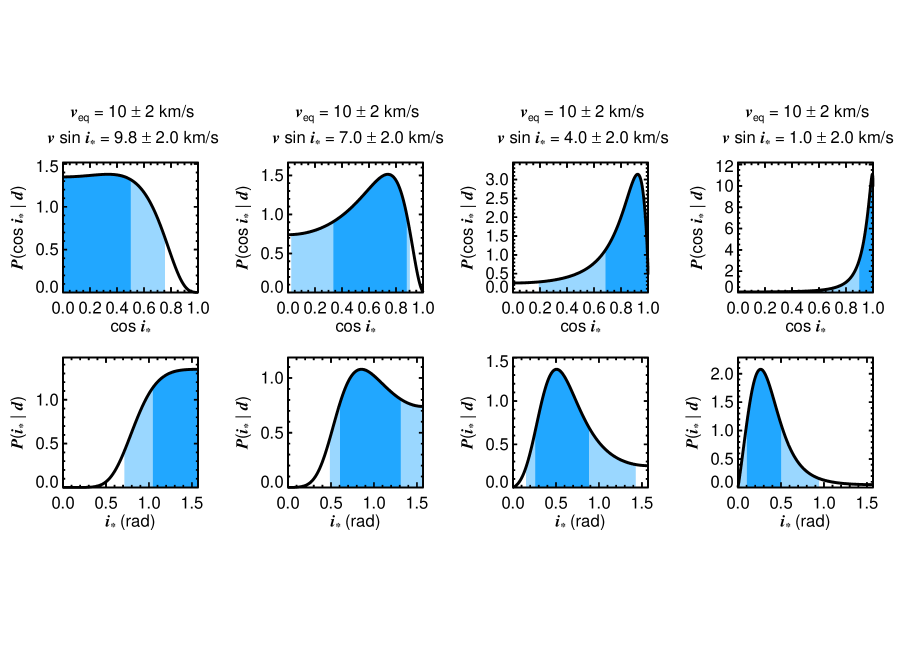
Figure 18: Posterior distributions for $\cos i_{*}$ and $i_{*}$ for the same examples from Masuda & Winn (2020) using our Equations A11 and A12. Shaded regions correspond to 68.3% and 95.4% credible intervals.

A.2 Upper Limits on $v\sin i_{*}$

In some cases only an upper limit on $v\sin i_{*}$ is available. This can occur if absorption lines are not fully resolved by an instrument or if a star is rotating slowly. Here we derive analytical expressions for this scenario in a similar fashion as was carried out for normally distributed measurements of $v\sin i_{*}$ in Appendix A.1.

Following Equation 11 of Masuda & Winn (2020), the posterior distribution of $\cos i_{*}$ can be written as an integral over $v\sin i$:

$${}P(\cos i_{*}\mid d)\propto\frac{\mathcal{P}(\cos i_{*})}{\sqrt{1-\cos i_{*}^{2}}}\int\mathcal{L}_{v_{\mathrm{eq}}}\Big{(}\frac{v\sin i_{*}}{\sqrt{1-\cos i_{*}^{2}}}\Big{)}\,\mathcal{L}_{v\sin i_{*}}(v\sin i_{*})\,\mathcal{P}_{v_{\mathrm{eq}}}\Big{(}\frac{v\sin i_{*}}{\sqrt{1-\cos i_{*}^{2}}}\Big{)}\,d\big{(}v\sin i_{*}\big{)}$$ (A13)

For an upper limit $l$ on the projected rotational velocity, its likelihood function is simply a uniform distribution from 0 km s^-1 to $l$ km s^-1: $\mathcal{L}_{v\sin i_{*}}(v\sin i_{*})$ $\sim$ $\mathcal{U}(v\sin i_{*}=0,v\sin i_{*}=l)$ km s^-1. This is equivalent to placing limits on the definite integral over $v\sin i_{*}$ from 0 to $l$. The likelihood function for the equatorial velocity, $\mathcal{L}_{v_{\mathrm{eq}}}(v\sin i_{*}/\sqrt{1-\cos i_{*}^{2}})$, is approximately normally distributed following Equation A4 if the rotation period is measured to a precision of $\lesssim$20%. Adopting an isotropic prior for $\mathcal{P}(\cos i_{*})$ and a uniform prior for $v_{\mathrm{eq}}$, Equation A13 becomes

$${}P(\cos i_{*}\mid d)\propto\int_{v\sin i_{*}=0}^{v\sin i_{*}=l}\frac{1}{\sqrt{2\pi}s}e^{-\frac{1}{2}\big{(}\frac{v\sin i_{*}-m}{s}\big{)}^{2}}\,d\big{(}v\sin i_{*}\big{)}$$ (A14)

where $m=\frac{2\pi R_{*}}{P_{\mathrm{rot}}}\sqrt{1-\cos i_{*}^{2}}$, $s=\sigma_{v_{\mathrm{eq}}}\sqrt{1-\cos i_{*}^{2}}$, and $\sigma_{v_{\mathrm{eq}}}=\frac{2\pi R_{*}}{P_{\mathrm{rot}}}\sqrt{\big{(}\frac{\sigma_{R_{*}}}{R_{*}}\big{)}^{2}+\big{(}\frac{\sigma_{P_{\mathrm{rot}}}}{P_{\mathrm{rot}}}\big{)}^{2}}$. Equation A14 is an integral over a Gaussian, the solution of which takes the following form:

$${}P(\cos i_{*}\mid d)\propto\mathrm{erf}\big{(}\frac{l-m}{\sqrt{2}\,s}\big{)}+\mathrm{erf}\big{(}\frac{m}{\sqrt{2}\,s}\big{)}$$ (A15)

and simplifies to

$${}P(\cos i_{*}\mid d)\propto\mathrm{erf}\Big{(}\frac{l-\frac{2\pi R_{*}}{P_{\mathrm{rot}}}\sqrt{1-\cos i_{*}^{2}}}{\sqrt{2}\,\sigma_{v_{\mathrm{eq}}}\sqrt{1-\cos i_{*}^{2}}}\Big{)}+\mathrm{erf}\Big{(}\frac{\sqrt{2}\,\pi R_{*}}{\sigma_{v_{\mathrm{eq}}}P_{\mathrm{rot}}}\Big{)}$$ (A16)

Therefore, for an upper limit on $v\sin i_{*}$ of $l$ km s^-1, the posterior distribution for $\cos i_{*}$ is simply proportional to the sum of two error functions.

Similarly, for the posterior of the inclination $i_{*}$, a variable transformation from $\cos i_{*}$ to $i_{*}$ gives

$${}P(i_{*}\mid d)\propto\sin i_{*}\times\Big{(}\mathrm{erf}\Big{(}\frac{l-\frac{2\pi R_{*}}{P_{\mathrm{rot}}}\sin i_{*}}{\sqrt{2}\,\sigma_{v_{\mathrm{eq}}}\sin i_{*}}\Big{)}+\mathrm{erf}\Big{(}\frac{\sqrt{2}\,\pi R_{*}}{\sigma_{v_{\mathrm{eq}}}P_{\mathrm{rot}}}\Big{)}\Big{)}.$$ (A17)

Several examples using Equations A16 and A17 are shown in Figure 19 following Masuda & Winn (2020). As in Appendix A.1, we use $R_{*}$ = 1.0 $\pm$ 0.1 $R_{\odot}$ and $P_{\mathrm{rot}}$ = 5.059 $\pm$ 0.88 d for this exercise. For a star with $v_{\mathrm{eq}}$ = 10 $\pm$ 2 km s^-1, we vary the upper limit of a hypothetical $v\sin i_{*}$ measurement from 2.5 km s^-1 to 30 km s^-1. As the upper limit moves beyond the equatorial rotational velocity, the posterior distribution of $\cos i_{*}$ tends to unity and for $i_{*}$ it tends to an isotropic distribution.

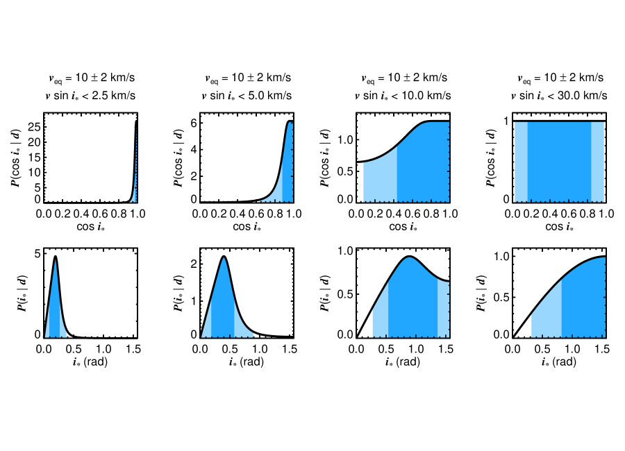
Figure 19: Same as Figure 18 but for examples of upper limits on $v\sin i_{*}$ from Masuda & Winn (2020) using our Equations A16 and A17. Shaded regions correspond to 68.3% and 95.4% credible intervals.

Appendix B Notes on Individual Stars

1RXS J034231.8+121622 This young mid-M dwarf is a likely member of the Hyades cluster (Kuzuhara et al. 2022). Its brown dwarf companion was found by Bowler et al. (2015a) and the latest orbit for the pair is determined in Bowler et al. (2020a). Our $v\sin i_{*}$ measurement of 5.1 $\pm$ 2.3 km s^-1 agrees with the upper limit of 7 km s^-1 from López-Valdivia et al. (2019). Likewise, our rotation period of 7.3 $\pm$ 0.3 d agrees with the value of 7.44 d from Newton et al. (2016).

2MASS J01033563–5515561: This low-mass hierarchical triple system comprises a close visual binary (AB) with an unresolved spectral type of M5–M6 and a wide 12–14 $M_{\mathrm{Jup}}$ accreting L-dwarf companion, 2MASS J01033563–5515561 b (Delorme et al. 2013; Eriksson et al. 2020; Betti et al. 2022). The light curve from two TESS sectors shows a strong periodic signal at 0.1664 $\pm$ 0.0003 d (3.994 $\pm$ 0.007 hr), which is consistent with fast rotation expected as a low-mass member of the $\approx$45 Myr Tuc-Hor young moving group (Kraus et al. 2014b). It is unclear which member of the binary is producing the observed modulations, but their near-equal flux ratios implies that they share similar physical properties.

To estimate their radii, we adopt an effective temperature of 2980 $\pm$ 75 K and $J$-band bolometric correction of 1.99 mag for young stars from Herczeg & Hillenbrand (2015) for 2MASS J01033563–5515561 A, which corresponds to young M5 stars. Assuming the B component is slightly cooler with a spectral type of M5.5, this corresponds to $T_{\mathrm{eff}}$ = 2920 $\pm$ 75 K and BC_J=2.01 mag. The absolute $J$-band magnitude of 2MASS J01033563–5515561 A is $M_{J}$ = 7.36 $\pm$ 0.05 mag (Delorme et al. 2013), which corresponds to a bolometric magnitude of $M_{\mathrm{bol}}$ = 9.35 $\pm$ 0.05 mag, a luminosity of $\log{L_{\mathrm{bol}}/L_{\odot}}$ = –1.84 $\pm$ 0.02 dex, and a radius of $R_{*}$ = 0.45 $\pm$ 0.03 $R_{\odot}$. The properties are similar for B: $M_{J}$ = 7.56 $\pm$ 0.05 mag (Delorme et al. 2013), $M_{\mathrm{bol}}$ = 9.57 $\pm$ 0.05 mag, $\log{L_{\mathrm{bol}}/L_{\odot}}$ = –1.93 $\pm$ 0.02 dex, and a radius of $R_{*}$ = 0.43 $\pm$ 0.02 $R_{\odot}$.

For the inclination analysis we assume the properties of A, although given the consistent radii the results would be similar for B. We find a stellar inclination of $i_{*}$=8.9${}^{+0.9}_{-1.3}\arcdeg$. In the future this measurement may be compared with the orbital angular momentum of the AB binary and, in principle, both the spin and orbit of the companion.

2MASS J01225093–2439505: This M3.5 star is a member of the AB Dor young moving group and hosts an imaged L4 substellar companion with a mass near the deuterium-burning limit (Bowler et al. 2013; Hinkley et al. 2015).

2MASS J01225093–2439505 has an inferred equatorial rotational velocity of 12.4 $\pm$ 1.0 km s^-1, which is inconsistent with the projected rotational velocity of 18.1 $\pm$ 0.5 km s^-1. The equatorial rotational velocity is based on a radius of 0.37 $\pm$ 0.03 $R_{\odot}$ from Stassun et al. (2019) and a rotation period of 1.493 $\pm$ 0.017 d from our analysis of the TESS light curve spanning two sectors. Note that this rotation period is nearly identical to the value of 1.49 $\pm$ 0.02 d determined by Bryan et al. (2020b) from a single TESS sector. The inconsistency between $v_{\mathrm{eq}}$ and $v\sin i_{*}$ implies that either the radius is too small, the rotation period is overestimated, the $v\sin i_{*}$ value is overestimated, or some combination of these.

The TESS light curve covers about 26 period cycles and shows regular single-mode modulations in Sector 3 followed by double-peaked modulations in Sector 30 with different peak amplitudes. Because of this double-peaked structure, which seems to trace two dominant groups of starspots at different longitudes, it is unlikely that the signal itself is an alias of a true underlying signal (as was discussed for LP 261-75 in Section 3.3). However, it is possible that mid-latitude starspots coupled with strong differential rotation could cause light curve modulations that are longer than the equatorial period, which might account for the discrepancy between $v_{\mathrm{eq}}$ and $v\sin i_{*}$.

It is also possible that the radius is underestimated. If the radius is the sole origin of the discrepancy between $v_{\mathrm{eq}}$ and $v\sin i_{*}$, a size of $\approx$0.53 $R_{\odot}$ would be needed to reconcile the two values. We recompute the radius using the apparent 2MASS $J$-band magnitude of 10.084 $\pm$ 0.028 mag, a $J$-band bolometric correction of 1.885 mag (midway between M3 and M4 from Herczeg & Hillenbrand 2015), an effective temperature of 3300 K (Herczeg & Hillenbrand 2015), and a $Gaia$ DR3-based distance of 33.74 $\pm$ 0.03 pc (Gaia Collaboration et al. 2022). This yields a bolometric magnitude of $M_{\mathrm{bol}}$ = 9.33 $\pm$ 0.05 mag, a luminosity of $\log{L_{\mathrm{bol}}/L_{\odot}}$ = –1.83 $\pm$ 0.02 dex, and a radius of $R_{*}$ = 0.37 $\pm$ 0.02 $R_{\odot}$—in good agreement with the TIC value from Stassun et al. (2019).

Finally, it is also possible that the $v\sin i_{*}$ value of 2MASS J01225093-2439505 may be overestimated. Our adopted value of 18.1 $\pm$ 0.5 km s^-1 is a weighted average of 14.2 $\pm$ 3.2 km s^-1 from Malo et al. (2014) and 18.2 $\pm$ 0.5 km s^-1 from Bryan et al. (2020b). Additional measurements of rotational broadening for this star would help clarify the nature of the discrepancy between $v_{\mathrm{eq}}$ and $v\sin i_{*}$.

FU Tau: FU Tau A is a young accreting late-M dwarf in the Taurus star-forming complex (Jones & Herbig 1979) which may be driving a large molecular outflow (Monin et al. 2013; although see Wu et al. 2020 for an alternate interpretation of the line emission). Its wide companion, FU Tau B, was discovered by Luhman et al. (2009) and is expected to have a mass near the deuterium-burning boundary.

The inferred mass and radius of FU Tau A is highly sensitive to the measured spectral type, extinction, effective temperature, and system age; values of 0.05–0.2 $M_{\odot}$ and 0.55–1.8 $R_{\odot}$ have been previously estimated (Luhman et al. 2009; Stelzer et al. 2010; Stelzer et al. 2013; Bulger et al. 2014). The parallax of FU Tau A in $Gaia$ DR3 (Gaia Collaboration et al. 2016; Gaia Collaboration et al. 2022) is 7.835 $\pm$ 0.075 mas, which corresponds to a distance estimate of 126.4 $\pm$ 1.0 pc (Bailer-Jones et al. 2021). This is about 10% closer than the 140 pc value that was often used in the past for Taurus members that lacked direct distance measurements, including FU Tau. We therefore re-derive the fundamental parameters of FU Tau A following a similar procedure as in Stelzer et al. (2013) using an (extinction-corrected) $J$-band bolometric correction and the revised distance.

Here we use a $J$-band bolometric correction of BC_J = 2.045 mag from Herczeg & Hillenbrand (2015), which is intermediate between young M6 and M7 stars and assumes a spectral type of M6.5 (Stelzer et al. 2013; Herczeg & Hillenbrand 2014) for FU Tau A. The optical extinction of $A_{V}$ = 0.5 $\pm$ 0.5 mag from Stelzer et al. (2013) corresponds to a $J$-band extinction of $A_{J}$ = 0.17 $\pm$ 0.11 mag based on infrared interstellar reddening law in Tokunaga (2000). This gives an absolute $J$-band magnitude of $M_{J}$ = 5.10 $\pm$ 0.12 mag for FU Tau A, a bolometric magnitude of $M_{\mathrm{bol}}$ = 7.15 $\pm$ 0.12 mag, a bolometric luminosity of $\log{L_{\mathrm{bol}}/L_{\odot}}$ = –0.96 $\pm$ 0.05 dex, and a radius of $R_{*}$ = 1.4 $\pm$ 0.1 $R_{\odot}$. These values rely on an effective temperature of $T_{\mathrm{eff}}$ = 2815 $\pm$ 75 K for a young M6.5 star (Herczeg & Hillenbrand 2015).

Based on the periodicity at 3.93 d we find from the TESS light curve, we infer an inclination of $i_{*}$=75${}^{+14}_{-5}\arcdeg$. The mm disk around FU Tau was detected by Wu et al. (2020) with ALMA but was not spatially resolved in that data. In the future, the inclination of FU Tau A’s disk and FU Tau B’s spin orientation may be compared with the inclination measured here.

FW Tau: FW Tau is a binary pair of young low-mass stars in the Taurus star-forming complex. The pair has equal flux ratio, implying similar physical properties, and shows significant orbital motion since 1989 (Schaefer et al. 2014). Bowler et al. (2014) found a spectral type of M6 $\pm$ 1 and modest extinction of $A_{V}$=0.4${}^{+1.3}_{-0.4}$ mag. A faint companion was found with HST imaging by White & Ghez (2001) and confirmed to be comoving by Kraus et al. (2014a), however follow-up studies suggest FW Tau C may be a brown dwarf or a low-mass star with an edge-on disk (Bowler et al. 2014; Kraus et al. 2015; Caceres et al. 2015; Wu & Sheehan 2017; Mora et al. 2020).

We compute the radii of FW Tau A and B by assuming each component is identical in luminosity and effective temperature. No parallax is available in $Gaia$ DR3 for FW Tau, presumably because of its binary nature, so we adopt a characteristic distance of 140 $\pm$ 10 pc for Taurus (Kenyon et al. 1994). Using a bolometric correction of 2.03 mag and $T_{\mathrm{eff}}$ = 2860 $\pm$ 75 K from Herczeg & Hillenbrand (2015), an optical extinction of $A_{V}$ = 0.4 mag (implying a $J$-band extinction of $A_{J}$ = 0.11 mag following Tokunaga 2000), and an apparent magnitude decomposed into equal-brightness individual magnitudes of $J$ = 11.1 $\pm$ 0.05 mag, we find $M_{J}$ = 5.25 $\pm$ 0.16 mag, $M_{\mathrm{bol}}$ = 7.28 $\pm$ 0.16 mag, $\log{L_{\mathrm{bol}}/L_{\odot}}$ = –1.01 $\pm$ 0.06 dex, and a radius of $R_{*}$ = 1.28 $\pm$ 0.11 $R_{\odot}$.

Our stellar rotation period of 0.91 d agrees well with the value of 0.906 d found by Chen et al. (2020) using $g$-band photometry from the Zwicky Transient Factory. They also report an $r$-band period of 0.475 d, which is probably an alias of the true rotation period. Combined with the $v\sin i_{*}$ of 49.2 $\pm$ 0.7 km s^-1 from Kounkel et al. (2019), the resulting posterior stellar inclination distribution peaks at $i_{*}$=44$\arcdeg$ and the 68% credible interval spans 39–49$\arcdeg$. Although the orbit of AB is not yet well constrained (Schaefer et al. 2014), its inclination and the properties of FW Tau C such as its disk inclination and spin inclination can eventually be compared with this stellar inclination to shed light on the formation of this hierarchical multiple system.

Gl 229: This nearby (5.7614 $\pm$ 0.0006 pc; Gaia Collaboration et al. 2022) M1 star hosts the first T dwarf companion to have been directly imaged (Nakajima et al. 1994; Oppenheimer et al. 1995; Oppenheimer 2014). With over 25 years of relative and absolute astrometry, the orbit and dynamical mass of Gl 229 B have now been exquisitely measured (Brandt et al. 2020; Brandt et al. 2021b; Feng et al. 2022).

The equatorial velocity of 1.0 $\pm$ 0.2 km s^-1 that we infer for Gl 229 is slightly (but significantly) smaller than its $v\sin i_{*}$ value of 2.8 $\pm$ 0.4 km s^-1, which is based on a compilation of projected rotational velocities from the literature (see Table 4). Most of the literature values do not include estimates of the measurement uncertainties, so these are grouped into a single value following the procedure outlined in Section 4.3. Note that our adopted value is dominated by the measurement of 2.6 $\pm$ 0.4 km s^-1 from Hojjatpanah et al. (2019), which is more heavily weighted because of its small reported uncertainties.

Most of these published $v\sin i_{*}$ measurements indicate that Gl 229 is a slow rotator, which is consistent with its old age (2–6 Gyr; Brandt et al. 2020), lack of activity signatures, and long rotation period of 27 d (Suarez Mascareno et al. 2016). Several $v\sin i_{*}$ measurements fall below 2 km s^-1 (Glebocki & Gnacinski (2005); Reiners 2007; Reiners et al. 2022), which at this level becomes very challenging to determine because it can be difficult to separate contributions to line broadening from rotation, microturbulence, and macroturbulence. The resulting obliquity constraint for Gl 229 may be suffer from a systematic bias because of an overestimated $v\sin i_{*}$ value.

The disagreement could also stem from the radius estimate or the photometric rotation period measurement. The radius of 0.55 $\pm$ 0.06 $R_{\odot}$ we adopt is similar to several other estimates such as 0.58 $\pm$ 0.05 $R_{\odot}$ from Houdebine et al. (2016) and 0.52 $\pm$ 0.02 $R_{\odot}$ from Schweitzer et al. (2019). An independent rotation period measurement would also be valuable for this star to compare with the 27 d value found by Suarez Mascareno et al. (2016).

SR 12 AB: SR 12 AB (2MASS J16271951–2441403, ROXs 21) is a close resolved binary (Simon et al. 1987) and a well-established member of the $\rho$ Ophiuchus cloud complex (e.g., Bouvier & Appenzeller 1992). Kuzuhara et al. (2011) discovered a widely separated companion, SR 12 c, with a mass near the deuterium-burning limit. SR 12 c was later found to have an accretion disk (Santamaría-Miranda et al. 2017; Martinez & Kraus 2022) with a dust mass of about one lunar mass based on a sub-mm detection with ALMA (Wu et al. 2022).

Here we derive the radius of SR 12 A using the Stefan-Boltzmann relation, but results are expected to be similar if the photometric rotation originates from SR 12 B. Schaefer et al. (2018) measured a flux ratio in the narrow-band Keck/NIRC2 $J_{\mathrm{cont}}$ filter of 0.951 $\pm$ 0.006, or 0.055 $\pm$ 0.006 mag. The apparent integrated-light $J$-band magnitude of SR 12 is 9.424 $\pm$ 0.023 mag (Cutri et al. 2003), which decomposes into apparent magnitudes of $J_{A}$ = 10.149 $\pm$ 0.023 mag and $J_{B}$ = 10.204 $\pm$ 0.023 mag. A parallax of 8.9034 $\pm$ 0.4288 mas ($d$ = 112 $\pm$ 5 pc; Bailer-Jones et al. 2018) is listed in Gaia DR2, but no parallax is present in DR3, likely because orbital motion of the binary is evident in the updated astrometry (the excess astrometric noise parameter is 7.121 mas but no RUWE value is listed). We therefore instead use the Gaia-based distance of 138.4 $\pm$ 2.6 pc inferred by Ortiz-León et al. (2018) for other members of the L1688 cloud. Adopting a spectral type of M0 from Wilking et al. (2005) implies an effective temperature of $T_{\mathrm{eff}}$ = 3900 $\pm$ 125 K (Herczeg & Hillenbrand 2015). Here we assume the $J$-band extinction of $A_{J}$ = 0.5 $\pm$ 0.2 mag from Kuzuhara et al. (2011). This implies an extinction-corrected absolute magnitude of $M_{J}$ = 3.95 $\pm$ 0.21 mag, a bolometric magnitude of $M_{\mathrm{bol}}$ = 5.61 $\pm$ 0.21 mag, a bolometric luminosity of $\log{L_{\mathrm{bol}}/L_{\odot}}$ = –0.34 $\pm$ 0.08 dex, and a radius of $R_{*}$ = 1.48 $\pm$ 0.17 $R_{\odot}$.

For this study we adopt the rotation period of 3.918 d found by Rebull et al. (2018) from K2, which is similar to the period of 3.927 d from Kiraga (2012) and 3.516 d from Grankin et al. (2008). Note that Jayasinghe et al. (2018) report a period of 7.849 d using light curves from the All-Sky Automated Survey for Supernovae (ASAS-SN); this is about twice the value from Rebull et al. (2018) so one is probably an alias of the true period. The cadence of ASAS-SN is every few days, whereas $K2$ is much finer ($\approx$30 min) and therefore should be more reliable.

Combining our radius estimate with the rotation period and adopted $v\sin i_{*}$ value of 27 $\pm$ 11 km s^-1 (Table 4) yields a broad inclination constraint that only slightly deviates from the $\sin i_{*}$ prior. Much of this is caused by the large uncertainty in projected rotational velocity. Orbital motion of AB has been detected but is not yet well determined (Schaefer et al. 2018); in the future the binary orbital plane and the spin inclination of the wide companion (Bryan et al. 2020a) can be compared with this host inclination to test for alignment.

TWA 5 Aab: TWA 5Aab is a M2 member of the $\approx$10 Myr TW Hydrae association. The brown dwarf companion TWA 5 B was found by Webb et al. (1999) and Lowrance et al. (1999), and the host was later resolved into a close visual binary by Macintosh et al. (2001).

Köhler et al. (2013) measured a dynamical mass of 0.9 $\pm$ 0.1 $M_{\odot}$ for the total mass of TWA 5Aab and a mass ratio of 1.3, implying individual masses of about 0.4 $M_{\odot}$  and 0.5 $M_{\odot}$ of the Ab and Aa components, respectively—albeit with large uncertainties. The radius of TWA 5 is listed as 0.40 $\pm$ 0.07 $R_{\odot}$ in Stassun et al. (2018), but this value differs substantially from theoretical expectations, perhaps because TWA 5 is a close binary. For example, solar-metallicity MIST models (Dotter 2016; Choi et al. 2016) predict a radius of 0.88 $R_{\odot}$ for a 0.5 $M_{\odot}$ star at 10 Myr. We instead adopt the weighted mean of radius estimates from Stassun et al. (2019) for two other coeval stars in the TWA association with the same spectral type of M2, TWA 7 (0.917 $\pm$ 0.119 $R_{\odot}$) and TWA 10 (0.860 $\pm$ 0.114 $R_{\odot}$). Following the discussion in Section 4.6, we also add a 7% uncertainty in quadrature with the original error estimates. This yields 0.89 $\pm$ 0.10 $R_{\odot}$.

Appendix C TESS light curves

Figures 20–27 show TESS light curves for host stars in our sample with periodic variations consistent with rotational modulation. Full light curves are shown in the left panels with breaks between non-contiguous sectors. The middle panels depict the Generalized Lomb-Scargle periodogram with the most prominent peak highlighted. The corresponding phased light curves and binned phased curves are displayed in the right panels. Starspot evolution is apparent for many targets.

Individual TESS sectors and rotation period measurements can be found in Table 3.3. A full description of the light curve extraction and reduction is summarized in Section 3.3. The observations used in this analysis can be accessed from MAST via https://doi.org/10.17909/t9-r086-e880 (catalog https://doi.org/10.17909/t9-r086-e880) and https://doi.org/10.17909/t9-wpz1-8s54 (catalog https://doi.org/10.17909/t9-wpz1-8s54).

Figure 20: Normalized TESS light curves and Generalized Lomb-Scargle periodograms for 1RXS J0342+1216, 2MASS J01033563–5515561, 2MASS J01225093–2439505, 2MASS J02155892–0929121, 2MASS J02192210–3925225, and 2MASS J04372171+2651014. For each light curve the strongest periodogram peak is marked with a dotted vertical line. Phased light curves are shown in the right panel with median binned phases denoted by cyan circles.

Figure 21: TESS light curves and periodograms for AB Pic, ASAS J212528–8138.5, BD+21 2486 AB, CD–35 2722, FU Tau, and FW Tau.

Figure 22: TESS light curves and periodograms for G 196-3, G 203-50, GJ 504, GJ 3305 AB, GSC 00568-01752, and GSC 08047-00232.

Figure 23: TESS light curves and periodograms for GU Psc, HD 116402, HD 129683, HD 130948, HD 16270, and HD 203030.

Figure 24: TESS light curves periodograms for HD 37216, HD 49197, HD 65486, HD 8291, HD 97334, and HD 984.

Figure 25: TESS light curves and periodograms for ksi UMa, L 34-26, LP 261-75 (Sectors 21 and 48), LP 261-75 (Sector 21), LP 261-75 (Sector 48), and LP 903-20.

Figure 26: TESS light curves and periodograms for PDS 70, PM J02133+3648, PZ Tel, Ross 458 AB, SDSS J130432.93+090713.7, and TWA 5 Aab.

Figure 27: TESS light curves and periodograms for TYC 8984-2245-1, TYC 8998-760-1, UCAC4 070-020389, VHS J125601.92–125723.9 AB, and Wolf 1130.

Appendix D Projected Rotational Velocities

$v\sin i_{*}$ values for substellar host stars with rotation periods are compiled from literature and our own new observations in Table 4. When available, $N$ independent measurements for the same star are combined into a single adopted value by computing a weighted mean and standard deviation:

$$\mu=\frac{\sum_{i=1}^{N}\mu_{i}/\sigma_{i}^{2}}{\sum_{i=1}^{N}1/\sigma_{i}^{2}}$$ (D1)

and

$$\sigma=\sqrt{\frac{1}{\sum_{i=1}^{N}1/\sigma_{i}^{2}}}.$$ (D2)

In some cases, projected rotational velocities are reported in the literature at precisions below 1%. These would dominate over other measurements with more typical uncertainties (5–20%) when computing a weighted mean. Because of the difficulty in separating the effects of microturbulence, macroturbulence, and rotational broadening, we conservatively set a floor of $\sigma_{v\sin i_{*}}$/ $v\sin i_{*}$ = 0.01 when computing the weighted mean.

In many instances $v\sin i_{*}$ values are reported without associated uncertainties. In these cases, when more than one are identified, we merge these into a single measurement by computing a robust mean and standard deviation following Beers et al. (1990).

Table 4: Adopted Projected Rotational Velocities.

	$v\sin i_{*}$
Name	(km s-1)	Reference
1RXS J034231.8+121622	5.1 $\pm$ 2.3	This work
1RXS J034231.8+121622	5.1 $\pm$ 2.3	Adopted
1RXS J160929.1–210524	8.2 $\pm$ 1.3	This work
1RXS J160929.1–210524	8.2 $\pm$ 1.3	Adopted
2MASS J01033563–5515561	35.2 $\pm$ 7.0	Malo et al. (2014)
2MASS J01033563–5515561	19.2 $\pm$ 2.4	Kraus et al. (2014b)
2MASS J01033563–5515561	20.9 $\pm$ 2.3	Adopted
2MASS J01225093–2439505	14.2 $\pm$ 3.2	Malo et al. (2014)
2MASS J01225093–2439505	18.2 $\pm$ 0.5	Bryan et al. (2020b)
2MASS J01225093–2439505	18.1 $\pm$ 0.5	Adopted
2MASS J02155892–0929121	17.6 $\pm$ 1.9	Malo et al. (2014)
2MASS J02155892–0929121	9.9 $\pm$ 0.9	Kraus et al. (2014b)
2MASS J02155892–0929121	15.7 $\pm$ 1.3	Fouqué et al. (2018)
2MASS J02155892–0929121	12.5 $\pm$ 0.7	Adopted
2MASS J04372171+2651014	22.54 $\pm$ 0.14	Gaidos et al. (2021)
2MASS J04372171+2651014	22.54 $\pm$ 0.14	Adopted
2MASS J02192210–3925225	6.5 $\pm$ 0.4	Kraus et al. (2014b)
2MASS J02192210–3925225	6.5 $\pm$ 0.4	Adopted
2MASS J16103196–1913062	5.6 $\pm$ 1.7	Dahm et al. (2012)
2MASS J16103196–1913062	5.6 $\pm$ 1.7	Adopted
2MASS J23513366+3127229	15 $\pm$ 2	This work
2MASS J23513366+3127229	12.9 $\pm$ 1.3	Malo et al. (2014)
2MASS J23513366+3127229	12.3 $\pm$ 0.8	Fouqué et al. (2018)
2MASS J23513366+3127229	12.7 $\pm$ 0.7	Adopted
51 Eri	69 $\pm$ 3	This work
51 Eri	71.8 $\pm$ 3.6	Reiners & Schmitt (2003)
51 Eri	57.4 $\pm$ 1.7	Zúñiga-Fernández et al. (2021)
51 Eri	70.0 $\pm$ 1.7	Saffe et al. (2021)
51 Eri	65.19 $\pm$ 0.17	Swastik et al. (2021)
51 Eri	80.9	Glebocki & Gnacinski (2005)
51 Eri	84	Royer et al. (2002)
51 Eri	95	Silva et al. (2009)
51 Eri	48.6	Grandjean et al. (2021)
51 Eri	81.2	Luck (2017)
51 Eri	73	Abt & Morrell (1995)
51 Eri	65.2 $\pm$ 0.6	Adopted
AB Pic	11.5 $\pm$ 0.1	Torres et al. (2006)
AB Pic	12.0 $\pm$ 0.9	Zúñiga-Fernández et al. (2021)
AB Pic	10.35 $\pm$ 0.06	Swastik et al. (2021)
AB Pic	10.8	Glebocki & Gnacinski (2005)
AB Pic	9.1	Grandjean et al. (2021)
AB Pic	10.87 $\pm$ 0.08	Adopted
ASAS J212528–8138.5	44.8 $\pm$ 4.2	Malo et al. (2014)
ASAS J212528–8138.5	43.5 $\pm$ 1.2	Torres et al. (2006)
ASAS J212528–8138.5	43.6 $\pm$ 1.2	Adopted
BD+21 55	2.1 $\pm$ 1.0	Kiefer et al. (2019)
BD+21 55	2.1 $\pm$ 1.0	Adopted
CD–35 2722	13.0 $\pm$ 0.4	Torres et al. (2006)
CD–35 2722	13.0 $\pm$ 1.5	Zúñiga-Fernández et al. (2021)
CD–35 2722	13.0 $\pm$ 0.4	Adopted
FU Tau	17.4 $\pm$ 0.3	Kounkel et al. (2019)
FU Tau	20 $\pm$ 5	Stelzer et al. (2013)
FU Tau	17.4 $\pm$ 0.3	Adopted
FW Tau	49.2 $\pm$ 0.7	Kounkel et al. (2019)
FW Tau	49.2 $\pm$ 0.7	Adopted
G 196-3	16.8 $\pm$ 1.7	This work
G 196-3	20 $\pm$ 5	Schlieder et al. (2012)
G 196-3	15.0	Glebocki & Gnacinski (2005)
G 196-3	17.2	Jeffers et al. (2018)
G 196-3	16.6 $\pm$ 1.1	Adopted
G 204-39	2.0 $\pm$ 1.1	Fouqué et al. (2018)
G 204-39	2.0 $\pm$ 1.1	Adopted
GJ 3305	15.22 $\pm$ 0.37	Jeffers et al. (2018)
GJ 3305	5.88 $\pm$ 0.47	Zúñiga-Fernández et al. (2021)
GJ 3305	3.2	Liebing et al. (2021)
GJ 3305	6.5	Houdebine (2010)
GJ 3305	5.0	Silva et al. (2009)
GJ 3305	5.3	Messina et al. (2010)
GJ 3305	11.4 $\pm$ 0.3	Adopted
Gl 229	4.5 $\pm$ 1.4	This work
Gl 229	2.61 $\pm$ 0.41	Hojjatpanah et al. (2019)
Gl 229	1.6	Glebocki & Gnacinski (2005)
Gl 229	1.0	Reiners (2007)
Gl 229	2.63	Houdebine et al. (2016)
Gl 229	9.0	López-Valdivia et al. (2019)
Gl 229	3.0	Pace et al. (2003)
Gl 229	6.4	Schröder et al. (2009)
Gl 229	2.0	Shan et al. (2021)
Gl 229	2.3	Liebing et al. (2021)
Gl 229	0.5	Reiners et al. (2022)
Gl 229	19.12	White et al. (2007)
Gl 229	2.63	Houdebine (2010)
Gl 229	2.8 $\pm$ 0.4	Adopted
Gl 504	7.76 $\pm$ 0.19	This work
Gl 504	4.5 $\pm$ 0.3	Reiners & Schmitt (2003)
Gl 504	7.2 $\pm$ 1.1	Eiff & Reiners (2012)
Gl 504	7.1 $\pm$ 0.3	Gonzalez et al. (2010)
Gl 504	6 $\pm$ 1	D’Orazi et al. (2017)
Gl 504	5.47 $\pm$ 0.17	Swastik et al. (2021)
Gl 504	6.6	Glebocki & Gnacinski (2005)
Gl 504	7.4	Valenti & Fischer (2005)
Gl 504	4.5	Schröder et al. (2009)
Gl 504	10.64	Martínez-Arnáiz et al. (2011)
Gl 504	7.1	Herrero et al. (2012)
Gl 504	5.8	Grandjean et al. (2021)
Gl 504	9.0	Luck (2017)
Gl 504	3.0	Takeda et al. (2005)
Gl 504	6.3 $\pm$ 0.1	Adopted
GQ Lup	6.8 $\pm$ 0.4	Guenther et al. (2005)
GQ Lup	5 $\pm$ 1	Donati et al. (2012)
GQ Lup	6.33 $\pm$ 0.07	Swastik et al. (2021)
GQ Lup	6.34 $\pm$ 0.07	Adopted
GSC 06214-00210	6.7 $\pm$ 0.4	This work
GSC 06214-00210	4.24 $\pm$ 0.05	Swastik et al. (2021)
GSC 06214-00210	4.29 $\pm$ 0.05	Adopted
GSC 08047-00232	19.8 $\pm$ 1.0	Torres et al. (2006)
GSC 08047-00232	20.0 $\pm$ 0.8	Zúñiga-Fernández et al. (2021)
GSC 08047-00232	19.9 $\pm$ 0.6	Adopted
GU Psc	23.8 $\pm$ 3.1	This work
GU Psc	23.7 $\pm$ 2.2	Malo et al. (2014)
GU Psc	23.7 $\pm$ 1.8	Adopted
HD 116402	38 $\pm$ 2	Chen et al. (2011)
HD 116402	33.2	Glebocki & Gnacinski (2005)
HD 116402	35	Cutispoto et al. (2002)
HD 116402	33	Kiraga (2012)
HD 116402	34.7 $\pm$ 1.0	Adopted
HD 129683	38 $\pm$ 3	Chen et al. (2011)
HD 129683	38 $\pm$ 3	Adopted
HD 130948	6.3	Glebocki & Gnacinski (2005)
HD 130948	6.8	Valenti & Fischer (2005)
HD 130948	6.0	Brewer et al. (2016)
HD 130948	6.0	Mishenina et al. (2008)
HD 130948	8.54	Martínez-Arnáiz et al. (2010)
HD 130948	6.8	Vican (2012)
HD 130948	7.8	Luck (2017)
HD 130948	6.3	Luck (2017)
HD 130948	7.0	Eiroa et al. (2013)
HD 130948	6.8 $\pm$ 0.9	Adopted
HD 16270	3.34 $\pm$ 0.07	Soto & Jenkins (2018)
HD 16270	3.7 $\pm$ 1.1	Soto & Jenkins (2018)
HD 16270	10.85	Martínez-Arnáiz et al. (2010)
HD 16270	3.34	Liebing et al. (2021)
HD 16270	3.34 $\pm$ 0.07	Adopted
HD 19467	3.3 $\pm$ 0.4	This work
HD 19467	1.6 $\pm$ 0.5	Crepp et al. (2014)
HD 19467	1.37 $\pm$ 0.14	Santos et al. (2016)
HD 19467	1.81 $\pm$ 0.18	Soto & Jenkins (2018)
HD 19467	1.92 $\pm$ 0.15	Soto & Jenkins (2018)
HD 19467	2.2 $\pm$ 0.5	Soto & Jenkins (2018)
HD 19467	1.1 $\pm$ 0.3	Soto & Jenkins (2018)
HD 19467	0.9	Glebocki & Gnacinski (2005)
HD 19467	1.5	Valenti & Fischer (2005)
HD 19467	1.4	Brewer et al. (2016)
HD 19467	1.3	Brewer et al. (2016)
HD 19467	1.0	Nordstrom et al. (2004)
HD 19467	1.554	Silva et al. (2020),
HD 19467	5.00	Liebing et al. (2021)
HD 19467	1.68 $\pm$ 0.08	Adopted
HD 203030	9.9 $\pm$ 2.0	Herrero et al. (2012)
HD 203030	6.3 $\pm$ 0.3	Frasca et al. (2018)
HD 203030	6.6 $\pm$ 0.8	Frasca et al. (2018)
HD 203030	5.62 $\pm$ 0.14	Swastik et al. (2021)
HD 203030	9.9	Strassmeier et al. (2000)
HD 203030	10.0	White et al. (2007)
HD 203030	7.4	Luck (2017)
HD 203030	6.8	Glebocki & Gnacinski (2005)
HD 203030	6.8	Brewer et al. (2016)
HD 203030	5.81 $\pm$ 0.12	Adopted
HD 3651	1.15 $\pm$ 0.5	Butler et al. (2006)
HD 3651	2.2 $\pm$ 0.5	López-Santiago et al. (2010)
HD 3651	2.2 $\pm$ 0.8	Herrero et al. (2012)
HD 3651	1.1 $\pm$ 0.3	Marsden et al. (2014)
HD 3651	1.6 $\pm$ 0.5	Gonzalez et al. (2010)
HD 3651	0.6	Glebocki & Gnacinski (2005)
HD 3651	1.5	Fischer & Valenti (2005)
HD 3651	8	López-Valdivia et al. (2019)
HD 3651	1.25	Rice & Brewer (2020)
HD 3651	1.1	Valenti & Fischer (2005)
HD 3651	11.97	Martínez-Arnáiz et al. (2010)
HD 3651	6.79	Martínez-Arnáiz et al. (2010)
HD 3651	4.1	Luck (2017)
HD 3651	1.4 $\pm$ 0.2	Adopted
HD 37216	5.8 $\pm$ 2.0	Herrero et al. (2012)
HD 37216	4.2	Glebocki & Gnacinski (2005)
HD 37216	3.35	Rice & Brewer (2020)
HD 37216	1.8	Valenti & Fischer (2005)
HD 37216	6.1	Strassmeier et al. (2000)
HD 37216	5.8	Strassmeier et al. (2000)
HD 37216	10.0	White et al. (2007)
HD 37216	5.6 $\pm$ 1.7	Adopted
HD 49197	23.1 $\pm$ 1.4	This work
HD 49197	24.44 $\pm$ 5.49	White et al. (2007)
HD 49197	23	Mizusawa et al. (2012)
HD 49197	20.7	Glebocki & Gnacinski (2005)
HD 49197	22.6 $\pm$ 1.0	Adopted
HD 8291	2.127 $\pm$ 0.19	Soto & Jenkins (2018)
HD 8291	2.30 $\pm$ 0.13	Santos et al. (2016)
HD 8291	3.0 $\pm$ 1.0	Dalal et al. (2021)
HD 8291	2.25 $\pm$ 1.1	Adopted
HD 97334	5.8 $\pm$ 0.5	Herrero et al. (2012)
HD 97334	5.4	Glebocki & Gnacinski (2005)
HD 97334	6.5	Valenti & Fischer (2005)
HD 97334	5.9	Brewer et al. (2016)
HD 97334	5.6	Mishenina et al. (2008)
HD 97334	7.74	Martínez-Arnáiz et al. (2010)
HD 97334	7.8	Luck (2017)
HD 97334	3.0	Bernacca & Perinotto (1970)
HD 97334	5.8 $\pm$ 0.5	Adopted
HD 984	38.7 $\pm$ 2.5	This work
HD 984	42.1 $\pm$ 1.7	White et al. (2007)
HD 984	39.3 $\pm$ 1.5	Zúñiga-Fernández et al. (2021)
HD 984	35.9	Glebocki & Gnacinski (2005)
HD 984	37.6	Valenti & Fischer (2005)
HD 984	21.05	Rice & Brewer (2020)
HD 984	38.6	Schröder et al. (2009)
HD 984	27.6	Grandjean et al. (2021)
HD 984	40.1 $\pm$ 1.0	Adopted
HIP 70319	1.3 $\pm$ 0.4	Herrero et al. (2012)
HIP 70319	3.8	Luck (2017)
HIP 70319	1.3	Glebocki & Gnacinski (2005)
HIP 70319	1.1	Valenti & Fischer (2005)
HIP 70319	0.1	Brewer et al. (2016)
HIP 70319	1.56	Takeda et al. (2010)
HIP 70319	2.0	Eiroa et al. (2013)
HIP 70319	1.3 $\pm$ 0.4	Adopted
HN Peg	10.6 $\pm$ 0.3	Marsden et al. (2014)
HN Peg	8.8 $\pm$ 0.2	Herrero et al. (2012)
HN Peg	10.4 $\pm$ 0.4	Eiff & Reiners (2012)
HN Peg	8.73 $\pm$ 0.06	Swastik et al. (2021)
HN Peg	9.9	Glebocki & Gnacinski (2005)
HN Peg	10.6	Valenti & Fischer (2005)
HN Peg	13	Cutispoto et al. (2002)
HN Peg	4.7	Mishenina et al. (2008)
HN Peg	12.81	Martínez-Arnáiz et al. (2010)
HN Peg	9.5	Mishenina et al. (2012)
HN Peg	9.7	Eiroa et al. (2013)
HN Peg	7.8	Grandjean et al. (2021)
HN Peg	10.1	Reiners et al. (2022)
HN Peg	11.2	Luck (2017)
HN Peg	8.92 $\pm$ 0.08	Adopted
HR 7672	4.1 $\pm$ 0.8	Herrero et al. (2012)
HR 7672	4.8	Glebocki & Gnacinski (2005)
HR 7672	3.6	Valenti & Fischer (2005)
HR 7672	2.3	Brewer et al. (2016)
HR 7672	5.0	Pace et al. (2003)
HR 7672	2.6	Mishenina et al. (2008)
HR 7672	8.06	Martínez-Arnáiz et al. (2010)
HR 7672	5.38	Martínez-Arnáiz et al. (2010)
HR 7672	8.27	Martínez-Arnáiz et al. (2010)
HR 7672	2.6	Mishenina et al. (2012)
HR 7672	5.6	Luck (2017)
HR 7672	2.3	Baum et al. (2022)
HR 7672	4	Takeda et al. (2005)
HR 7672	4.2 $\pm$ 0.7	Adopted
ksi Uma	1	Meyer et al. (1998)
ksi Uma	3	Meyer et al. (1998)
ksi Uma	2.8	Strassmeier et al. (1999)
ksi Uma	8.3	Luck (2017)
ksi Uma	3.6	Glebocki & Gnacinski (2005)
ksi Uma	3.7 $\pm$ 1.4	Adopted
L 34-26	7.4 $\pm$ 0.42	Hojjatpanah et al. (2019)
L 34-26	8.1 $\pm$ 1.2	Torres et al. (2006)
L 34-26	7.5 $\pm$ 0.4	Adopted
LkCa 15	13.9 $\pm$ 1.2	Nguyen et al. (2012)
LkCa 15	16.8 $\pm$ 0.2	Swastik et al. (2021)
LkCa 15	12.5	Glebocki & Gnacinski (2005)
LkCa 15	14.8	Hartmann et al. (1987)
LkCa 15	12.3	Hartmann et al. (1987)
LkCa 15	13.1	Hartmann et al. (1987)
LkCa 15	11.8	Hartmann et al. (1987)
LkCa 15	16.62 $\pm$ 0.19	Adopted
PDS 70	16.0 $\pm$ 0.5	Thanathibodee et al. (2020)
PDS 70	17.3 $\pm$ 0.1	Swastik et al. (2021)
PDS 70	17.16 $\pm$ 0.16	Adopted
PM J02133+3648	25.1 $\pm$ 1.1	Fouqué et al. (2018)
PM J02133+3648	25.1 $\pm$ 1.1	Adopted
PZ Tel	69.0 $\pm$ 0.1	Torres et al. (2006)
PZ Tel	58 $\pm$ 7	Herrero et al. (2012)
PZ Tel	55 $\pm$ 13	Zúñiga-Fernández et al. (2021)
PZ Tel	73 $\pm$ 5	Jenkins et al. (2012)
PZ Tel	58 $\pm$ 7	Soderblom et al. (1998)
PZ Tel	77.5 $\pm$ 2.8	Scholz et al. (2007)
PZ Tel	68	Barnes et al. (2000)
PZ Tel	70	Cutispoto et al. (2002)
PZ Tel	63	Reza & Pinzon (2004)
PZTel	70	Randich et al. (1993)
PZ Tel	66.2	Glebocki & Gnacinski (2005)
PZ Tel	54.1	Grandjean et al. (2021)
PZ Tel	69.3 $\pm$ 0.7	Adopted
Ross 458	11.5 $\pm$ 1.3	This work
Ross 458	9.75 $\pm$ 0.3	Houdebine (2010)
Ross 458	10.0	Glebocki & Gnacinski (2005)
Ross 458	9.75	Houdebine et al. (2016)
Ross 458	13.0	López-Valdivia et al. (2019)
Ross 458	5.90	Rice & Brewer (2020)
Ross 458	9.7	Browning et al. (2010)
Ross 458	11.0	Donati et al. (2008)
Ross 458	9.8 $\pm$ 0.3	Adopted
ROXs 12	8.2 $\pm$ 0.7	Bowler et al. (2017)
ROXs 12	7.20 $\pm$ 0.04	Swastik et al. (2021)
ROXs 12	7.21 $\pm$ 0.07	Adopted
RXJ1602.8–2401B	16.5 $\pm$ 1.3	Dahm et al. (2012)
RXJ1602.8–2401B	16.5 $\pm$ 1.3	Adopted
SR 12	38.7	Glebocki & Gnacinski (2005)
SR 12	19.87	Jönsson et al. (2020)
SR 12	21	Herbig & Bell (1988)
SR 12	27 $\pm$ 11	Adopted
TWA 5 Aab	53.5 $\pm$ 3.5	Torres et al. (2006)
TWA 5 Aab	59.2	Glebocki & Gnacinski (2005)
TWA 5 Aab	54	Silva et al. (2009)
TWA 5 A	55.0 $\pm$ 2.5	Adopted
TYC 8984-2245-1	19.3 $\pm$ 0.5	Torres et al. (2006)
TYC 8984-2245-1	19.3 $\pm$ 0.5	Adopted
VHS J125601.92–125723.9	75 $\pm$ 3	Bryan et al. (2018)
VHS J125601.92–125723.9	75 $\pm$ 3	Adopted
Wolf 1130	12.7	Houdebine (2010)
Wolf 1130	15	Jenkins et al. (2009)
Wolf 1130	13.9 $\pm$ 1.6	Adopted

References

- Abt & Morrell (1995) Abt, H. A., & Morrell, N. I. 1995, Astrophysical Journal Supplement, 99, 135
- Adams (2010) Adams, F. C. 2010, Annu. Rev. Astro. Astrophys., 48, 47
- Aerts (2021) Aerts, C. 2021, Reviews of Modern Physics, 93, 015001
- Albrecht et al. (2009) Albrecht, S., Reffert, S., Snellen, I. A. G., & Winn, J. N. 2009, Nature, 461, 373
- Albrecht et al. (2013) Albrecht, S., Winn, J. N., Marcy, G. W., et al. 2013, ApJ, 771, 11
- Albrecht et al. (2012) Albrecht, S., Winn, J. N., Johnson, J. A., et al. 2012, The Astrophysical Journal, 757, 18
- Albrecht et al. (2022) Albrecht, S. H., Dawson, R. I., & Winn, J. N. 2022, Publications of the Astronomical Society of the Pacific, 134, 082001
- Allers et al. (2010) Allers, K. N., Liu, M. C., Dupuy, T. J., & Cushing, M. C. 2010, The Astrophysical Journal, 715, 561
- Anderson et al. (2017) Anderson, K. R., Lai, D., & Storch, N. I. 2017, Monthly Notices of the Royal Astronomical Society, 467, 3066
- Anderson et al. (2016) Anderson, K. R., Storch, N. I., & Lai, D. 2016, MNRAS, 456, 3671
- Ansdell et al. (2020) Ansdell, M., Gaidos, E., Hedges, C., et al. 2020, MNRAS, 492, 572
- Artigau et al. (2015) Artigau, E., Gagné, J., Faherty, J., et al. 2015, ApJ, 806, 254
- Avallone et al. (2022) Avallone, E. A., Tayar, J. N., Saders, J. L. v., et al. 2022, The Astrophysical Journal, 930, 7
- Bailer-Jones et al. (2021) Bailer-Jones, C. A. L., Rybizki, J., Fouesneau, M., Demleitner, M., & Andrae, R. 2021, The Astronomical Journal, 161, 147
- Bailer-Jones et al. (2018) Bailer-Jones, C. A. L., Rybizki, J., Fouesneau, M., Mantelet, G., & Andrae, R. 2018, The Astronomical Journal, 156, 58
- Bailey et al. (2016) Bailey, E., Batygin, K., & Brown, M. E. 2016, The Astronomical Journal, 152, 126
- Bailey & Fabrycky (2019) Bailey, N., & Fabrycky, D. 2019, The Astronomical Journal, 158, 94
- Bailey et al. (2014) Bailey, V., Meshkat, T., Reiter, M., et al. 2014, The Astrophysical Journal, 780, L4
- Baliunas et al. (1996) Baliunas, S., Sokoloff, D., & Soon, W. 1996, ApJ, 457, L99
- Barnes et al. (2005) Barnes, J. R., Cameron, A. C., Donati, J.-F., et al. 2005, MNRAS, 357, L1
- Barnes et al. (2000) Barnes, J. R., Cameron, A. C., James, D. J., & Donati, J. F. 2000, MNRAS, 314, 162
- Bate (2009) Bate, M. R. 2009, Monthly Notices of the Royal Astronomical Society, 392, 590
- Bate (2012) —. 2012, Monthly Notices of the Royal Astronomical Society, 419, 3115
- Bate et al. (2002) Bate, M. R., Bonnell, I. A., & Bromm, V. 2002, Monthly Notices of the Royal Astronomical Society, 332, L65
- Bate et al. (2010) Bate, M. R., Lodato, G., & Pringle, J. E. 2010, Monthly Notices of the Royal Astronomical Society, 401, 1505
- Batygin (2012) Batygin, K. 2012, Nature, 491, 418
- Batygin & Adams (2013) Batygin, K., & Adams, F. C. 2013, ApJ, 778, 169
- Batygin et al. (2020) Batygin, K., Adams, F. C., Batygin, Y. K., & Petigura, E. A. 2020, The Astronomical Journal, 159, 101
- Baum et al. (2022) Baum, A. C., Wright, J. T., Luhn, J. K., & Isaacson, H. 2022, The Astronomical Journal, 163, 183
- Beers et al. (1990) Beers, T. C., Flynn, K., & Gebhardt, K. 1990, Astronomical Journal, 100, 32
- Belle (2012) Belle, G. T. v. 2012, The Astronomy and Astrophysics Review, 20, 51
- Benomar et al. (2018) Benomar, O., Bazot, M., Nielsen, M. B., et al. 2018, Science, 361, 1231
- Berdyugina (2005) Berdyugina, S. V. 2005, Living Reviews in Solar Physics, 2, 8
- Bernacca & Perinotto (1970) Bernacca, P. L., & Perinotto, M. 1970, CoAsi, 239, 1
- Best et al. (2021) Best, W. M. J., Liu, M. C., Magnier, E. A., & Dupuy, T. J. 2021, The Astronomical Journal, 161, 42
- Best et al. (2018) Best, W. M. J., Magnier, E. A., Liu, M. C., et al. 2018, The Astrophysical Journal Supplement Series, 234, 1
- Betti et al. (2022) Betti, S. K., Follette, K. B., Ward-Duong, K., et al. 2022, The Astrophysical Journal Letters, 935, L18
- Biller et al. (2010) Biller, B. A., Liu, M. C., Wahhaj, Z., et al. 2010, The Astrophysical Journal, 720, L82
- Blunt et al. (2017) Blunt, S., Nielsen, E. L., Rosa, R. J. D., et al. 2017, The Astronomical Journal, 153, 229
- Blunt et al. (2020) Blunt, S., Wang, J. J., Angelo, I., et al. 2020, The Astronomical Journal, 159, 89
- Bohn et al. (2020a) Bohn, A. J., Kenworthy, M. A., Ginski, C., et al. 2020a, Monthly Notices of the Royal Astronomical Society, 492, 431
- Bohn et al. (2020b) —. 2020b, The Astrophysical Journal Letters, 898, L16
- Bohn et al. (2021) Bohn, A. J., Ginski, C., Kenworthy, M. A., et al. 2021, Astronomy & Astrophysics, 648, A73
- Bonavita et al. (2022) Bonavita, M., Fontanive, C., Gratton, R., et al. 2022, Monthly Notices of the Royal Astronomical Society, 513, 5588
- Bonnefoy et al. (2018) Bonnefoy, M., Perraut, K., Lagrange, A.-M., et al. 2018, Astronomy and Astrophysics, 618, A63
- Boss (2006) Boss, A. P. 2006, The Astrophysical Journal, 637, L137
- Bouvier & Appenzeller (1992) Bouvier, J., & Appenzeller, I. 1992, ApJS, 92, 481
- Bouy et al. (2003) Bouy, H., Brandner, W., Martín, E. L., et al. 2003, The Astronomical Journal, 126, 1526
- Bowler (2016) Bowler, B. P. 2016, Publications of the Astronomical Society of the Pacific, 128, 102001
- Bowler et al. (2020a) Bowler, B. P., Blunt, S. C., & Nielsen, E. L. 2020a, Astronomical Journal, 159, 63
- Bowler et al. (2014) Bowler, B. P., Liu, M. C., Kraus, A. L., & Mann, A. W. 2014, The Astrophysical Journal, 784, 65
- Bowler et al. (2013) Bowler, B. P., Liu, M. C., Shkolnik, E. L., & Dupuy, T. J. 2013, The Astrophysical Journal, 774, 55
- Bowler et al. (2012) Bowler, B. P., Liu, M. C., Shkolnik, E. L., et al. 2012, The Astrophysical Journal, 753, 142
- Bowler et al. (2015a) Bowler, B. P., Liu, M. C., Shkolnik, E. L., & Tamura, M. 2015a, The Astrophysical Journal Supplement Series, 216, 7
- Bowler et al. (2020b) Bowler, B. P., Zhou, Y., Morley, C. V., et al. 2020b, The Astrophysical Journal Letters, 893, L30
- Bowler et al. (2015b) Bowler, B. P., Shkolnik, E. L., Liu, M. C., et al. 2015b, The Astrophysical Journal, 806, 62
- Bowler et al. (2017) Bowler, B. P., Kraus, A. L., Bryan, M. L., et al. 2017, The Astronomical Journal, 154, 165
- Bowler et al. (2018) Bowler, B. P., Dupuy, T. J., Endl, M., et al. 2018, The Astronomical Journal, 155, 159
- Brandt et al. (2021a) Brandt, G. M., Brandt, T. D., Dupuy, T. J., Li, Y., & Michalik, D. 2021a, The Astronomical Journal, 161, 179
- Brandt et al. (2021b) Brandt, G. M., Dupuy, T. J., Li, Y., et al. 2021b, The Astronomical Journal, 162, 301
- Brandt et al. (2019) Brandt, T. D., Dupuy, T. J., & Bowler, B. P. 2019, The Astronomical Journal, 158, 140
- Brandt et al. (2020) Brandt, T. D., Dupuy, T. J., Bowler, B. P., et al. 2020, The Astronomical Journal, 160, 196
- Brewer et al. (2016) Brewer, J. M., Fischer, D. A., Valenti, J. A., & Piskunov, N. 2016, The Astrophysical Journal Supplement Series, 225, 32
- Browning et al. (2010) Browning, M. K., Basri, G., Marcy, G. W., West, A. A., & Zhang, J. 2010, The Astronomical Journal, 139, 504
- Brun et al. (2017) Brun, A. S., Strugarek, A., Varela, J., et al. 2017, The Astrophysical Journal, 836, 192
- Bryan et al. (2018) Bryan, M. L., Benneke, B., Knutson, H. A., Batygin, K., & Bowler, B. P. 2018, Nature Astronomy, 128, 63
- Bryan et al. (2016) Bryan, M. L., Bowler, B. P., Knutson, H. A., et al. 2016, ApJ, 827, 100
- Bryan et al. (2021) Bryan, M. L., Chiang, E., Morley, C. V., Mace, G. N., & Bowler, B. P. 2021, The Astronomical Journal, 162, 217
- Bryan et al. (2020a) Bryan, M. L., Ginzburg, S., Chiang, E., et al. 2020a, The Astrophysical Journal, 905, 37
- Bryan et al. (2020b) Bryan, M. L., Chiang, E., Bowler, B. P., et al. 2020b, The Astronomical Journal, 159, 181
- Bulger et al. (2014) Bulger, J., Patience, J., Ward-Duong, K., et al. 2014, A&A, 570, A29
- Butler et al. (2006) Butler, R. P., Wright, J. T., Marcy, G. W., et al. 2006, The Astrophysical Journal, 646, 505
- Caceres et al. (2015) Caceres, C., Hardy, A., Schreiber, M. R., et al. 2015, The Astrophysical Journal Letters, 806, L22
- Caldwell et al. (2020) Caldwell, D. A., Tenenbaum, P., Twicken, J. D., et al. 2020, RNAAS, 4, 201
- Campante et al. (2016) Campante, T. L., Lund, M. N., Kuszlewicz, J. S., et al. 2016, ApJ, 819, 85
- Canto Martins et al. (2020) Canto Martins, B. L., Gomes, R. L., Messias, Y. S., et al. 2020, The Astrophysical Journal Supplement Series, 250, 20
- Carson et al. (2013) Carson, J., Thalmann, C., Janson, M., et al. 2013, ApJL, 763, L32
- Chatterjee et al. (2008) Chatterjee, S., Ford, E. B., Matsumura, S., & Rasio, F. A. 2008, The Astrophysical Journal, 686, 580
- Chauvin et al. (2003) Chauvin, G., Thomson, M., Dumas, C., et al. 2003, A&A, 404, 157
- Chauvin et al. (2005) Chauvin, G., Lagrange, A.-M., Zuckerman, B., et al. 2005, A&A, 438, L29
- Chen et al. (2011) Chen, C. H., Mamajek, E. E., Bitner, M. A., et al. 2011, The Astrophysical Journal, 738, 122
- Chen et al. (2020) Chen, C. H., Su, K. Y. L., & Xu, S. 2020, Nature Astronomy, 4, 328
- Choi et al. (2016) Choi, J., Dotter, A., Conroy, C., et al. 2016, The Astrophysical Journal, 823, 102
- Chubak et al. (2012) Chubak, C., Marcy, G., Fischer, D. A., et al. 2012, arXiv:1207.6212
- Crepp et al. (2014) Crepp, J. R., Johnson, J. A., Howard, A. W., et al. 2014, ApJ, 781, 29
- Crepp et al. (2012) Crepp, J. R., Johnson, J. A., Fischer, D. A., et al. 2012, The Astrophysical Journal, 751, 97
- Cruz et al. (2003) Cruz, K. L., Reid, I. N., Liebert, J., Kirkpatrick, J. D., & Lowrance, P. J. 2003, The Astronomical Journal, 126, 2421
- Cutispoto et al. (2002) Cutispoto, G., Pastori, L., Pasquini, L., et al. 2002, Astronomy & Astrophysics, 384, 491
- Cutri et al. (2003) Cutri, R. M., Skrutskie, M. F., Dyk, S. V., et al. 2003, The 2MASS All-Sky Catalog of Point Sources, University of Massachusetts and Infrared Processing and Analysis Center; IPAC/California Institute of Technology
- Czekala et al. (2015) Czekala, I., Andrews, S. M., Jensen, E. L. N., et al. 2015, The Astrophysical Journal, 806, 154
- Daffern-Powell et al. (2022) Daffern-Powell, E. C., Parker, R. J., & Quanz, S. P. 2022, Monthly Notices of the Royal Astronomical Society, 514, 920
- Dahm et al. (2012) Dahm, S. E., Slesnick, C. L., & White, R. J. 2012, The Astrophysical Journal, 745, 56
- Dalal et al. (2021) Dalal, S., Kiefer, F., Hébrard, G., et al. 2021, Astronomy & Astrophysics, 651, A11
- Davies et al. (2014) Davies, C. L., Gregory, S. G., & Greaves, J. S. 2014, Monthly Notices of the Royal Astronomical Society, 444, 1157
- Dawson (2014) Dawson, R. I. 2014, The Astrophysical Journal Letters, 790, L31
- Dawson et al. (2011) Dawson, R. I., Murray-Clay, R. A., & Fabrycky, D. C. 2011, The Astrophysical Journal, 743, L17
- Deacon et al. (2016) Deacon, N. R., Schlieder, J. E., & Murphy, S. J. 2016, Monthly Notices of the Royal Astronomical Society, 457, 3191
- Deacon et al. (2012) Deacon, N. R., Liu, M. C., Magnier, E. A., et al. 2012, The Astrophysical Journal, 755, 94
- Deacon et al. (2014) —. 2014, ApJ, 792, 119
- Deacon et al. (2017) Deacon, N. R., Magnier, E. A., Liu, M. C., et al. 2017, Monthly Notices of the Royal Astronomical Society, 467, 1126
- Delorme et al. (2013) Delorme, P., Gagné, J., Girard, J. H., et al. 2013, A&A, 553, L5
- Delorme et al. (2017) Delorme, P., Schmidt, T., Bonnefoy, M., et al. 2017, Astronomy & Astrophysics, 608, A79
- Donahue et al. (1996) Donahue, R. A., Saar, S. H., & Baliunas, S. L. 1996, Astrophysical Journal, 466, 384
- Donati et al. (2008) Donati, J.-F., Morin, J., Petit, P., et al. 2008, Monthly Notices of the Royal Astronomical Society, 390, 545
- Donati et al. (2012) Donati, J. F., Gregory, S. G., Alencar, S. H. P., et al. 2012, Monthly Notices of the Royal Astronomical Society, 425, 2948
- D’Orazi et al. (2017) D’Orazi, V., Desidera, S., Gratton, R. G., et al. 2017, A&A, 598, A19
- Dotter (2016) Dotter, A. 2016, The Astrophysical Journal Supplement Series, 222, 8
- Drilling & Landolt (2000) Drilling, J. S., & Landolt, A. U. 2000, in Allen’s Astrophysical Quantities, 4th ed., ed. A. N. Cox (New York, NY: AIP Press; Springer 2000), 381
- Dupuy et al. (2022a) Dupuy, T. J., Brandt, G. M., & Brandt, T. D. 2022a, Monthly Notices of the Royal Astronomical Society, 509, 4411
- Dupuy & Kraus (2013) Dupuy, T. J., & Kraus, A. L. 2013, Science, 341, 1492
- Dupuy & Liu (2012) Dupuy, T. J., & Liu, M. C. 2012, The Astrophysical Journal Supplement, 201, 19
- Dupuy et al. (2022b) Dupuy, T. J., Liu, M. C., Evans, E. L., et al. 2022b, arXiv, 2208.08448
- Durisen et al. (2007) Durisen, R. H., Boss, A. P., Mayer, L., et al. 2007, in Protostars and Planets V, e. B. Reipurth, D. Jewitt, & K. Keil (Tucson, AZ: Univ. Arizona Press), 607
- Díaz-Francés & Rubio (2013) Díaz-Francés, E., & Rubio, F. J. 2013, Statistical Papers, 54, 309
- Eiff & Reiners (2012) Eiff, M. A.-v., & Reiners, A. 2012, Astronomy and Astrophysics, 542, A116
- Eiroa et al. (2013) Eiroa, C., Marshall, J. P., Mora, A., et al. 2013, A&A, 555, A11
- Epstein-Martin et al. (2022) Epstein-Martin, M., Becker, J., & Batygin, K. 2022, The Astrophysical Journal, 931, 42
- Eriksson et al. (2020) Eriksson, S. C., Torres, R. A., Janson, M., et al. 2020, Astronomy & Astrophysics, 638, L6
- Fabrycky & Tremaine (2007) Fabrycky, D., & Tremaine, S. 2007, The Astrophysical Journal, 669, 1298
- Fabrycky & Winn (2009) Fabrycky, D. C., & Winn, J. N. 2009, The Astrophysical Journal, 696, 1230
- Faherty et al. (2010) Faherty, J. K., Burgasser, A. J., West, A. A., et al. 2010, The Astronomical Journal, 139, 176
- Faramaz et al. (2021) Faramaz, V., Marino, S., Booth, M., et al. 2021, The Astronomical Journal, 161, 271
- Feigelson et al. (2006) Feigelson, E. D., Lawson, W. A., Stark, M., Townsley, L., & Garmire, G. P. 2006, AJ, 131, 1730
- Feng et al. (2022) Feng, F., Butler, R. P., Vogt, S. S., et al. 2022, The Astrophysical Journal Supplement Series, 262, 21
- Ferrer-Chávez et al. (2021) Ferrer-Chávez, R., Wang, J. J., & Blunt, S. 2021, The Astronomical Journal, 161, 241
- Fielding et al. (2015) Fielding, D. B., McKee, C. F., Socrates, A., Cunningham, A. J., & Klein, R. I. 2015, Monthly Notices of the Royal Astronomical Society, 450, 3306
- Fischer & Valenti (2005) Fischer, D. A., & Valenti, J. 2005, The Astrophysical Journal, 622, 1102
- Ford & Rasio (2008) Ford, E. B., & Rasio, F. A. 2008, The Astrophysical Journal, 686, 621
- Fouqué et al. (2018) Fouqué, P., Moutou, C., Malo, L., et al. 2018, Monthly Notices of the Royal Astronomical Society, 475, 1960
- Franson et al. (2022a) Franson, K., Bowler, B. P., Brandt, T. D., et al. 2022a, The Astronomical Journal, 163, 50
- Franson et al. (2022b) Franson, K., Bowler, B. P., Bonavita, M., et al. 2022b, arXiv, 2211.09840
- Frasca et al. (2018) Frasca, A., Guillout, P., Klutsch, A., et al. 2018, Astronomy & Astrophysics, 612, A96
- Gaia Collaboration et al. (2022) Gaia Collaboration, Vallenari, A., Brown, A. G. A., & Prusti, T. 2022, arxiv:2208.00211
- Gaia Collaboration et al. (2016) Gaia Collaboration, Prusti, T., Bruijne, J. H. J. d., et al. 2016, A&A, 595, A1
- Gaidos et al. (2021) Gaidos, E., Hirano, T., Kraus, A. L., et al. 2021, Monthly Notices of the Royal Astronomical Society, 512, 583
- Gaudi & Winn (2007) Gaudi, B. S., & Winn, J. N. 2007, The Astrophysical Journal, 655, 550
- Gauza et al. (2015) Gauza, B., Bejar, V. J. S., Pérez-Garrido, A., et al. 2015, The Astrophysical Journal, 804, 96
- Geballe et al. (2002) Geballe, T. R., Knapp, G. R., Leggett, S. K., et al. 2002, The Astrophysical Journal, 564, 466
- Gizis et al. (2001) Gizis, J. E., Kirkpatrick, J. D., & Wilson, J. C. 2001, The Astronomical Journal, 121, 2185
- Glebocki & Gnacinski (2005) Glebocki, R., & Gnacinski, P. 2005, yCat, 3244, 0
- Glebocki & Stawikowski (1997) Glebocki, R., & Stawikowski, A. 1997, A&A, 328, 579
- Goldman et al. (2010) Goldman, B., Marsat, S., Henning, T., Clemens, C., & Greiner, J. 2010, Monthly Notices of the Royal Astronomical Society, 405, 1140
- Gomes et al. (2013) Gomes, J. I., Pinfield, D. J., Marocco, F., et al. 2013, Monthly Notices of the Royal Astronomical Society, 431, 2745
- Gonzalez et al. (2010) Gonzalez, G., Carlson, M. K., & Tobin, R. W. 2010, PASJ, 403, 1368
- Grandjean et al. (2021) Grandjean, A., Lagrange, A.-M., Meunier, N., et al. 2021, Astronomy & Astrophysics, 650, A39
- Grankin et al. (2008) Grankin, K. N., Bouvier, J., Herbst, W., & Melnikov, S. Y. 2008, Astronomy & Astrophysics, 479, 827
- Gray (2005) Gray, D. F. 2005, The Observation and Analysis of Stellar Photospheres (3rd Ed.; Cambridge: Cambridge Univ. Press)
- Greaves et al. (2014) Greaves, J. S., Kennedy, G. M., Thureau, N., et al. 2014, MNRAS, 438, L31
- Guenther et al. (2005) Guenther, E. W., Neuhäuser, R., Wuchterl, G., et al. 2005, Astronomische Nachrichten, 326, 958
- Haffert et al. (2019) Haffert, S. Y., Bohn, A. J., Boer, J., et al. 2019, Nature Astronomy, 3, 749
- Hale (1994) Hale, A. 1994, The Astronomical Journal, 107, 306
- Hartman et al. (2011) Hartman, J. D., Bakos, G. A., Noyes, R. W., et al. 2011, The Astronomical Journal, 141, 166
- Hartmann et al. (1987) Hartmann, L. W., Soderblom, D. R., & Stauffer, J. R. 1987, AJ, 93, 907
- Hastings (1970) Hastings, W. 1970, Biometrika, 57, 97
- Heller (1993) Heller, C. H. 1993, The Astrophysical Journal, 408, 337
- Herbig & Bell (1988) Herbig, G. H., & Bell, K. R. 1988, in Third Catalog of Emission-Line Stars of the Orion Population, ed. G. H. Herbig & K. R. Bell, Vol. 3 (Santa Cruz, CA: Lick Observatory), 90
- Herczeg & Hillenbrand (2014) Herczeg, G. J., & Hillenbrand, L. A. 2014, ApJ, 786, 97
- Herczeg & Hillenbrand (2015) —. 2015, The Astrophysical Journal, 808, 23
- Herrero et al. (2012) Herrero, E., Ribas, I., Jordi, C., Guinan, E. F., & Engle, S. G. 2012, Astronomy and Astrophysics, 537, A147
- Hinkley (1969) Hinkley, D. 1969, PASJ, 56, 635
- Hinkley et al. (2015) Hinkley, S., Bowler, B. P., Vigan, A., et al. 2015, The Astrophysical Journal Letters, 805, L10
- Hinkley et al. (2022) Hinkley, S., Lacour, S., Marleau, G. D., et al. 2022, arXiv:2208.04867
- Hogg et al. (2010) Hogg, D. W., Myers, A. D., & Bovy, J. 2010, The Astrophysical Journal, 725, 2166
- Hojjatpanah et al. (2019) Hojjatpanah, S., Figueira, P., Santos, N. C., et al. 2019, Astronomy & Astrophysics, 629, A80
- Holt (1893) Holt. 1893, AstAp, 12, 646
- Horne (1986) Horne, K. 1986, Astronomical Society of the Pacific, 98, 609
- Houdebine (2010) Houdebine, E. R. 2010, Monthly Notices of the Royal Astronomical Society, 407, 1657
- Houdebine et al. (2016) Houdebine, E. R., Mullan, D. J., Paletou, F., & Gebran, M. 2016, The Astrophysical Journal, 822, 97
- Huang et al. (2020) Huang, C. X., Vanderburg, A., Pal, A., et al. 2020, RNAAS, 4, 204
- Huber et al. (2013) Huber, D., Carter, J. A., Barbieri, M., et al. 2013, Science, 342, 331
- Huber et al. (2017) Huber, D., Zinn, J., Bojsen-Hansen, M., et al. 2017, The Astrophysical Journal, 844, 102
- Husser et al. (2013) Husser, T. O., Berg, S. W.-v., Dreizler, S., et al. 2013, A&A, 553, A6
- Ireland et al. (2011) Ireland, M. J., Kraus, A., Martinache, F., Law, N., & Hillenbrand, L. A. 2011, The Astrophysical Journal, 726, 113
- Iriarte et al. (2021) Iriarte, Y. A., de Castro, M., & Gomez, H. W. 2021, Symmetry, 13, 269
- Irwin et al. (2018) Irwin, J. M., Charbonneau, D., Esquerdo, G. A., et al. 2018, The Astronomical Journal, 156, 140
- Janson (2010) Janson, M. 2010, Monthly Notices of the Royal Astronomical Society, 408, 514
- Janson et al. (2012) Janson, M., Jayawardhana, R., Girard, J. H., et al. 2012, ApJL, 758, L2
- Jayasinghe et al. (2018) Jayasinghe, T., Kochanek, C. S., Stanek, K. Z., et al. 2018, Monthly Notices of the Royal Astronomical Society, 477, 3145
- Jeffers et al. (2018) Jeffers, S. V., Schöfer, P., Lamert, A., et al. 2018, Astronomy & Astrophysics, 614, A76
- Jenkins et al. (2016) Jenkins, J. M., Twicken, J. D., McCauliff, S., et al. 2016, Proc. SPIE, 9913, 99133E
- Jenkins et al. (2009) Jenkins, J. S., Ramsey, L. W., Jones, H. R. A., et al. 2009, The Astrophysical Journal, 704, 975
- Jenkins et al. (2012) Jenkins, J. S., Pavlenko, Y. V., Ivanyuk, O., et al. 2012, Monthly Notices of the Royal Astronomical Society, 420, 3587
- Jennings & Chiang (2021) Jennings, R. M., & Chiang, E. 2021, Monthly Notices of the Royal Astronomical Society, 507, 5187
- Jones & Herbig (1979) Jones, B. F., & Herbig, G. H. 1979, AJ, 84, 1874
- Jones et al. (2016) Jones, J., White, R. J., Quinn, S., et al. 2016, The Astrophysical Journal Letters, 822, L3
- Jumper & Fisher (2013) Jumper, P. H., & Fisher, R. T. 2013, ApJ, 769, 9
- Justesen & Albrecht (2020) Justesen, A. B., & Albrecht, S. 2020, A&A, 642, A212
- Jönsson et al. (2020) Jönsson, H., Holtzman, J. A., Prieto, C. A., et al. 2020, The Astronomical Journal, 160, 120
- Kaye et al. (1999) Kaye, A. B., Handler, G., Krisciunas, K., Poretti, E., & Zerbi, F. M. 1999, Publications of the Astronomical Society of the Pacific, 111, 840
- Kendall et al. (2007) Kendall, T. R., Jones, H. R. A., Pinfield, D. J., et al. 2007, Monthly Notices of the Royal Astronomical Society, 374, 445
- Kenyon et al. (1994) Kenyon, S., Dobrzycka, D., & Hartmann, L. 1994, AJ, 108, 1872
- Keppler et al. (2018) Keppler, M., Benisty, M., Müller, A., et al. 2018, Astronomy and Astrophysics, 617, A44
- Keppler et al. (2019) Keppler, M., Teague, R., Bae, J., et al. 2019, Astronomy & Astrophysics, 625, A118
- Kiefer et al. (2019) Kiefer, F., Hébrard, G., Sahlmann, J., et al. 2019, Astronomy & Astrophysics, 631, A125
- Kiraga (2012) Kiraga, M. 2012, Acta Astronomica, 62, 67
- Kirkpatrick et al. (2001) Kirkpatrick, J. D., Dahn, C. C., Monet, D. G., et al. 2001, The Astronomical Journal, 121, 3235
- Kirkpatrick et al. (2000) Kirkpatrick, J. D., Reid, I. N., Liebert, J., et al. 2000, The Astronomical Journal, 120, 447
- Kirkpatrick et al. (2011) Kirkpatrick, J. D., Cushing, M. C., Gelino, C. R., et al. 2011, The Astrophysical Journal Supplement, 197, 19
- Knapp et al. (2004) Knapp, G. R., Leggett, S. K., Fan, X., et al. 2004, The Astronomical Journal, 127, 3553
- Konopacky et al. (2016) Konopacky, Q. M., Rameau, J., Duchene, G., et al. 2016, The Astrophysical Journal Letters, 829, L4
- Kounkel et al. (2019) Kounkel, M., Covey, K., Moe, M., et al. 2019, The Astronomical Journal, 157, 196
- Kraus et al. (2015) Kraus, A. L., Andrews, S. M., Bowler, B. P., et al. 2015, The Astrophysical Journal, 798, L23
- Kraus & Hillenbrand (2009) Kraus, A. L., & Hillenbrand, L. A. 2009, The Astrophysical Journal, 703, 1511
- Kraus & Ireland (2012) Kraus, A. L., & Ireland, M. J. 2012, The Astrophysical Journal, 745, 5
- Kraus et al. (2014a) Kraus, A. L., Ireland, M. J., Cieza, L. A., et al. 2014a, The Astrophysical Journal, 781, 20
- Kraus et al. (2014b) Kraus, A. L., Shkolnik, E. L., Allers, K. N., & Liu, M. C. 2014b, AJ, 147, 146
- Kraus et al. (2020) Kraus, S., Bouquin, J.-B. L., Kreplin, A., et al. 2020, The Astrophysical Journal Letters, 897, L8
- Kraus et al. (2022) Kraus, S., Mortimer, D., Chhabra, S., et al. 2022, SPIE, 12183, 121831S
- Kuzuhara et al. (2011) Kuzuhara, M., Tamura, M., Ishii, M., et al. 2011, The Astronomical Journal, 141, 119
- Kuzuhara et al. (2013) Kuzuhara, M., Tamura, M., Kudo, T., et al. 2013, The Astrophysical Journal, 774, 11
- Kuzuhara et al. (2022) Kuzuhara, M., Currie, T., Takarada, T., et al. 2022, The Astrophysical Journal Letters, 934, L18
- Köhler et al. (2013) Köhler, R., Ratzka, T., Petr-Gotzens, M. G., & Correia, S. 2013, A&A, 558, A80
- Lacour et al. (2021) Lacour, S., Wang, J. J., Rodet, L., et al. 2021, Astronomy & Astrophysics, 654, L2
- Lafrenière et al. (2008) Lafrenière, D., Jayawardhana, R., & Kerkwijk, M. H. v. 2008, The Astrophysical Journal, 689, L153
- Lagrange et al. (2019) Lagrange, A.-M., Meunier, N., Rubini, P., et al. 2019, Nature Astronomy, 3, 1135
- Lagrange et al. (2020) Lagrange, A.-M., Rubini, P., Nowak, M., et al. 2020, Astronomy and Astrophysics, 642, A18
- Lai et al. (2018) Lai, D., Anderson, K. R., & Pu, B. 2018, MNRAS, 475, 5231
- Lai et al. (2011) Lai, D., Foucart, F., & Lin, D. N. C. 2011, Monthly Notices of the Royal Astronomical Society, 412, 2790
- Lambrechts & Johansen (2012) Lambrechts, M., & Johansen, A. 2012, A&A, 544, A32
- Le Bouquin et al. (2009) Le Bouquin, J.-B., Absil, O., Benisty, M., et al. 2009, Astronomy & Astrophysics, 498, L41
- Liebing et al. (2021) Liebing, F., Jeffers, S. V., Reiners, A., & Zechmeister, M. 2021, Astronomy and Astrophysics, 654, A168
- Lightkurve Collaboration et al. (2018) Lightkurve Collaboration, Miranda, C. V. d., Hedges, C., et al. 2018, Lightkurve: Kepler and TESS time series analysis in Python, Astrophysics Source Code Library, ascl:1812.013
- Liu et al. (2016) Liu, M. C., Dupuy, T. J., & Allers, K. N. 2016, ApJ, 833, 1
- Liu et al. (2002) Liu, M. C., Fischer, D. A., Graham, J. R., et al. 2002, The Astrophysical Journal, 571, 519
- Liu et al. (2007) Liu, M. C., Leggett, S. K., & Chiu, K. 2007, The Astrophysical Journal, 660, 1507
- Louden et al. (2021) Louden, E. M., Winn, J. N., Petigura, E. A., et al. 2021, The Astronomical Journal, 161, 68
- Lovis & Pepe (2007) Lovis, C., & Pepe, F. 2007, A&A, 468, 1115
- Low & Lynden-Bell (1976) Low, C., & Lynden-Bell, D. 1976, Royal Astronomical Society, 176, 367
- Lowrance et al. (1999) Lowrance, P. J., McCarthy, C., Becklin, E. E., et al. 1999, The Astrophysical Journal, 512, L69
- Luck (2017) Luck, R. E. 2017, The Astronomical Journal, 153, 21
- Luhman et al. (2009) Luhman, K. L., Mamajek, E. E., Allen, P. R., Muench, A. A., & Finkbeiner, D. P. 2009, The Astrophysical Journal, 691, 1265
- Luhman et al. (2007) Luhman, K. L., Patten, B. M., Marengo, M., et al. 2007, The Astrophysical Journal, 654, 570
- López-Santiago et al. (2010) López-Santiago, J., Montes, D., Gálvez-Ortiz, M. C., et al. 2010, Astronomy & Astrophysics, 514, A97
- López-Valdivia et al. (2019) López-Valdivia, R., Mace, G. N., Sokal, K. R., et al. 2019, The Astrophysical Journal, 879, 105
- Mace et al. (2013) Mace, G. N., Kirkpatrick, J. D., Cushing, M. C., et al. 2013, ApJ, 777, 36
- Macintosh et al. (2015) Macintosh, B., Graham, J. R., Barman, T., et al. 2015, Science, 350, 64
- Macintosh et al. (2001) Macintosh, B. A., Max, C., Zuckerman, B., et al. 2001, Young Stars Near Earth: Progress and Prospects, 244, 309
- Maire et al. (2018) Maire, A.-L., Rodet, L., Lazzoni, C., et al. 2018, Astronomy & Astrophysics, 615, A177
- Maire et al. (2019) Maire, A. L., Rodet, L., Cantalloube, F., et al. 2019, A&A, 624, A118
- Maire et al. (2020) Maire, A. L., Molaverdikhani, K., Desidera, S., et al. 2020, Astronomy and Astrophysics, 639, A47
- Malo et al. (2014) Malo, L., Artigau, E., Doyon, R., et al. 2014, ApJ, 788, 81
- Mamajek (2012) Mamajek, E. E. 2012, The Astrophysical Journal, 754, L20
- Marcussen & Albrecht (2022) Marcussen, M. L., & Albrecht, S. H. 2022, The Astrophysical Journal, 933, 227
- Marino et al. (2015) Marino, S., Pérez, S., & Casassus, S. 2015, ApJL, 798, L44
- Marino et al. (2020) Marino, S., Zurlo, A., Faramaz, V., et al. 2020, Monthly Notices of the Royal Astronomical Society, 498, 1319
- Marois et al. (2008) Marois, C., Macintosh, B., Barman, T., et al. 2008, Science, 322, 1348
- Marois et al. (2010) Marois, C., Zuckerman, B., Konopacky, Q. M., Macintosh, B., & Barman, T. 2010, Nature, 372, 1
- Marsden et al. (2014) Marsden, S. C., Petit, P., Jeffers, S. V., et al. 2014, Monthly Notices of the Royal Astronomical Society, 444, 3517
- Martinez & Kraus (2022) Martinez, R. A., & Kraus, A. L. 2022, The Astronomical Journal, 163, 36
- Martínez-Arnáiz et al. (2011) Martínez-Arnáiz, R., López-Santiago, J., Crespo-Chacón, I., & Montes, D. 2011, Monthly Notices of the Royal Astronomical Society, 414, 2629
- Martínez-Arnáiz et al. (2010) Martínez-Arnáiz, R., Maldonado, J., Montes, D., Eiroa, C., & Montesinos, B. 2010, A&A, 520, A79
- Masuda (2022) Masuda, K. 2022, The Astrophysical Journal, 937, 94
- Masuda et al. (2021) Masuda, K., Petigura, E. A., & Hall, O. J. 2021, Monthly Notices of the Royal Astronomical Society, 510, 5623
- Masuda & Winn (2020) Masuda, K., & Winn, J. N. 2020, The Astronomical Journal, 159, 81
- Mawet et al. (2016) Mawet, D., Wizinowich, P., Dekany, R., et al. 2016, Proceedings of the SPIE, 9909, 99090D
- McLaughlin (1924) McLaughlin, D. B. 1924, The Astrophysical Journal, 60, 22
- Mellon et al. (2017) Mellon, S. N., Mamajek, E. E., Oberst, T. E., & Pecaut, M. J. 2017, The Astrophysical Journal, 844, 66
- Meshkat et al. (2015) Meshkat, T., Bonnefoy, M., Mamajek, E. E., et al. 2015, Monthly Notices of the Royal Astronomical Society, 453, 2379
- Messina et al. (2010) Messina, S., Desidera, S., Turatto, M., Lanzafame, A. C., & Guinan, E. F. 2010, A&A, 520, A15
- Metchev & Hillenbrand (2004) Metchev, S. A., & Hillenbrand, L. A. 2004, The Astrophysical Journal, 617, 1330
- Metchev & Hillenbrand (2006) —. 2006, The Astrophysical Journal, 651, 1166
- Metropolis et al. (1953) Metropolis, N., Rosenbluth, A., Rosenbluth, M., Teller, A., & Teller, E. 1953, The Journal of Chemical Physics, 21, 1087
- Meyer et al. (1998) Meyer, M. R., Edwards, S., Hinkle, K. H., & Strom, S. E. 1998, The Astrophysical Journal, 508, 397
- Milli et al. (2017) Milli, J., Hibon, P., Christiaens, V., et al. 2017, A&A, 597, L2
- Mishenina et al. (2008) Mishenina, T. V., Soubiran, C., Bienaymé, O., et al. 2008, Astronomy & Astrophysics, 489, 923
- Mishenina et al. (2012) Mishenina, T. V., Soubiran, C., Kovtyukh, V. V., Katsova, M. M., & Livshits, M. A. 2012, Astronomy & Astrophysics, 547, A106
- Mizusawa et al. (2012) Mizusawa, T. F., Rebull, L. M., Stauffer, J. R., et al. 2012, The Astronomical Journal, 144, 135
- Monin et al. (2013) Monin, J.-L., Whelan, E. T., Lefloch, B., Dougados, C., & Oliveira, C. A. d. 2013, A&A, 551, L1
- Montalto et al. (2021) Montalto, M., Piotto, G., Marrese, P. M., et al. 2021, Astronomy & Astrophysics, 653, A98
- Mora et al. (2020) Mora, A., Wu, Y.-L., Bowler, B. P., & Sheehan, P. 2020, RNAAS, 4, 9
- Morton & Johnson (2011) Morton, T. D., & Johnson, J. A. 2011, The Astrophysical Journal, 729, 138
- Morton & Winn (2014) Morton, T. D., & Winn, J. N. 2014, ApJ, 796, 47
- Mugrauer et al. (2006) Mugrauer, M., Seifahrt, A., Neuhäuser, R., & Mazeh, T. 2006, Monthly Notices RAS Letters, 373, L31
- Mugrauer et al. (2010) Mugrauer, M., Vogt, N., Neuhäuser, R., & Schmidt, T. O. B. 2010, A&A, 523, L1
- Muirhead et al. (2018) Muirhead, P. S., Dressing, C. D., Mann, A. W., et al. 2018, The Astronomical Journal, 155, 180
- Murphy et al. (2007) Murphy, M. T., Tzanavaris, P., Webb, J. K., & Lovis, C. 2007, PASJ, 378, 221
- Muñoz & Perets (2018) Muñoz, D. J., & Perets, H. B. 2018, The Astronomical Journal, 156, 253
- Müller et al. (2018) Müller, A., Keppler, M., Henning, T., et al. 2018, A&A, 617, L2
- Nagpal et al. (2022) Nagpal, V., Blunt, S., Bowler, B. P., et al. 2022, arXiv, 2211.02121
- Nakajima et al. (1994) Nakajima, T., Durrance, S. T., Golimowski, D. A., & Kulkarni, S. R. 1994, The Astrophysical Journal, 428, 797
- Nakajima et al. (1995) Nakajima, T., Oppenheimer, B. R., Kulkarni, S. R., et al. 1995, Nature, 378, 463
- Naud et al. (2014) Naud, M.-E., Artigau, E., Malo, L., et al. 2014, ApJ, 787, 5
- Nederlander et al. (2021) Nederlander, A., Hughes, A. M., Fehr, A. J., et al. 2021, The Astrophysical Journal, 917, 5
- Nelder & Mead (1965) Nelder, J. A., & Mead, R. 1965, The computer journal, 7, 308
- Neuhäuser et al. (2003) Neuhäuser, R., Guenther, E. W., Alves, J., et al. 2003, Astronomische Nachrichten
- Neuhäuser et al. (2005) Neuhäuser, R., Guenther, E. W., Wuchterl, G., et al. 2005, A&A, 435, L13
- Newton et al. (2016) Newton, E. R., Irwin, J., Charbonneau, D., et al. 2016, ApJ, 821, 93
- Nguyen et al. (2012) Nguyen, D. C., Brandeker, A., Kerkwijk, M. H. v., & Jayawardhana, R. 2012, The Astrophysical Journal, 745, 119
- Nguyen et al. (2021) Nguyen, M. M., Rosa, R. J. D., & Kalas, P. 2021, The Astronomical Journal, 161, 22
- Nielsen et al. (2019) Nielsen, E. L., Rosa, R. J. D., Macintosh, B., et al. 2019, The Astronomical Journal, 158, 13
- Nordstrom et al. (2004) Nordstrom, B., Mayor, M., Andersen, J., et al. 2004, A&A, 418, 989
- Nowak et al. (2020) Nowak, M., Lacour, S., Lagrange, A.-M., et al. 2020, Astronomy and Astrophysics, 642, L2
- Oelkers et al. (2018) Oelkers, R. J., Rodriguez, J. E., Stassun, K. G., et al. 2018, The Astronomical Journal, 155, 39
- Offner et al. (2016) Offner, S. S. R., Dunham, M. M., Lee, K. I., Arce, H. G., & Fielding, D. B. 2016, The Astrophysical Journal Letters, 827, L11
- Oliveira et al. (2015) Oliveira, A., Oliveira, T., Macías, S., & Antonio. 2015, AIP Conference Proceedings, 1648, 840005
- Oppenheimer (2014) Oppenheimer, B. R. 2014, in ”50 Years of Brown Dwarfs,” V. Joergens, ed., Astrophysics and Space Science Library, Volume 401, (Zurich: Springer), astro-ph.SR, 1404.4430v1
- Oppenheimer et al. (1995) Oppenheimer, B. R., Kulkarni, S. R., Matthews, K., & Nakajima, T. 1995, Science, 270, 1478
- Ortiz-León et al. (2018) Ortiz-León, G. N., Loinard, L., Dzib, S. A., et al. 2018, The Astrophysical Journal Letters, 869, L33
- O’Neil et al. (2019) O’Neil, K. K., Martinez, G. D., Hees, A., et al. 2019, The Astronomical Journal, 158, 4
- Pace et al. (2003) Pace, G., Pasquini, L., & Ortolani, S. 2003, Astronomy & Astrophysics, 401, 997
- Palma-Bifani et al. (2022) Palma-Bifani, P., Chauvin, G., Bonnefoy, M., et al. 2022, arXiv, 2211.01474
- Parker & Daffern-Powell (2022) Parker, R. J., & Daffern-Powell, E. C. 2022, Monthly Notices of the Royal Astronomical Society: Letters, 516, L91
- Parker & Quanz (2012) Parker, R. J., & Quanz, S. P. 2012, Monthly Notices of the Royal Astronomical Society, 419, 2448
- Pearce et al. (2019) Pearce, L. A., Kraus, A. L., Dupuy, T. J., et al. 2019, The Astronomical Journal, 157, 71
- Pecaut & Mamajek (2013) Pecaut, M. J., & Mamajek, E. E. 2013, The Astrophysical Journal Supplement Series, 208, 9
- Perets & Kouwenhoven (2012) Perets, H. B., & Kouwenhoven, M. B. N. 2012, The Astrophysical Journal, 750, 83
- Petigura et al. (2017) Petigura, E. A., Howard, A. W., Marcy, G. W., et al. 2017, The Astronomical Journal, 154, 107
- Phan‐Bao et al. (2008) Phan‐Bao, N., Bessell, M. S., Martín, E. L., et al. 2008, Monthly Notices of the Royal Astronomical Society, 383, 831
- Pinfield et al. (2012) Pinfield, D. J., Burningham, B., lodieu, N., et al. 2012, Monthly Notices of the Royal Astronomical Society, 422, 1922
- Potter et al. (2002) Potter, D., Martín, E. L., Cushing, M. C., et al. 2002, The Astrophysical Journal, 567, L133
- Queloz et al. (2000) Queloz, D., Eggenberger, A., Mayor, M., et al. 2000, A&A, 359, L13
- Radigan et al. (2008) Radigan, J., Lafrenière, D., Jayawardhana, R., & Doyon, R. 2008, The Astrophysical Journal, 689, 471
- Randich et al. (1993) Randich, S., Gratton, R., & Pallavicini, R. 1993, A&A, 273, 194
- Rebolo et al. (1998) Rebolo, R., Osorio, M. R. Z., Madruga, S., et al. 1998, Science, 282, 1309
- Rebull et al. (2018) Rebull, L. M., Stauffer, J. R., Cody, A. M., et al. 2018, The Astronomical Journal, 155, 196
- Reid et al. (2008) Reid, I. N., Cruz, K. L., Kirkpatrick, J. D., et al. 2008, The Astronomical Journal, 136, 1290
- Reid & Walkowicz (2006) Reid, I. N., & Walkowicz, L. M. 2006, The Publications of the Astronomical Society of the Pacific, 118, 671
- Reiners (2007) Reiners, A. 2007, Astronomy & Astrophysics, 467, 259
- Reiners & Schmitt (2003) Reiners, A., & Schmitt, J. H. M. M. 2003, Astronomy and Astrophysics, 398, 647
- Reiners et al. (2022) Reiners, A., Shulyak, D., Käpylä, P. J., et al. 2022, Astronomy & Astrophysics, 662, A41
- Reinhold & Gizon (2015) Reinhold, T., & Gizon, L. 2015, A&A, 583, A65
- Reinhold et al. (2013) Reinhold, T., Reiners, A., & Basri, G. 2013, A&A, 560, A4
- Reinhold et al. (2020) Reinhold, T., Shapiro, A. I., Solanki, S. K., et al. 2020, Science, 368, 518
- Reza & Pinzon (2004) Reza, R. d. l., & Pinzon, G. 2004, AJ, 128, 1812
- Rice & Brewer (2020) Rice, M., & Brewer, J. M. 2020, The Astrophysical Journal, 898, 119
- Ricker et al. (2015) Ricker, G. R., Winn, J. N., Vanderspek, R., et al. 2015, Proc. SPIE, 9143, 914320
- Rodriguez et al. (2017) Rodriguez, J. E., Ansdell, M., Oelkers, R. J., et al. 2017, The Astrophysical Journal, 848, 97
- Roettenbacher et al. (2016) Roettenbacher, R. M., Monnier, J. D., Korhonen, H., et al. 2016, Nature, 533, 217
- Rossiter (1924) Rossiter, R. A. 1924, Astrophysical Journal, 60, 15
- Royer et al. (2002) Royer, F., Grenier, S., Baylac, M. O., Gomez, A. E., & Zorec, J. 2002, Astronomy and Astrophysics, 393, 897
- Ruffio et al. (2019) Ruffio, J.-B., Macintosh, B., Konopacky, Q. M., et al. 2019, The Astronomical Journal, 158, 200
- Ruffio et al. (2021) Ruffio, J.-B., Konopacky, Q. M., Barman, T., et al. 2021, The Astronomical Journal, 162, 290
- Saffe et al. (2021) Saffe, C., Miquelarena, P., Alacoria, J., et al. 2021, Astronomy and Astrophysics, 647, A49
- Santamaría-Miranda et al. (2017) Santamaría-Miranda, A., Cáceres, C., Schreiber, M. R., et al. 2017, Monthly Notices of the Royal Astronomical Society, 475, 2994
- Santos et al. (2016) Santos, L. A. d., Meléndez, J., Nascimento, J.-D. d., et al. 2016, Astronomy and Astrophysics, 592, A156
- Savitzky & Golay (1964) Savitzky, A., & Golay, M. J. E. 1964, AnaCh, 36, 1627
- Schaefer et al. (2018) Schaefer, G. H., Prato, L., & Simon, M. 2018, The Astronomical Journal, 155, 109
- Schaefer et al. (2014) Schaefer, G. H., Prato, L., Simon, M., & Patience, J. 2014, The Astronomical Journal, 147, 157
- Schlaufman (2010) Schlaufman, K. C. 2010, ApJ, 719, 602
- Schlieder et al. (2012) Schlieder, J. E., Lépine, S., & Simon, M. 2012, The Astronomical Journal, 143, 80
- Scholz et al. (2007) Scholz, A., Coffey, J., Brandeker, A., & Jayawardhana, R. 2007, The Astrophysical Journal, 662, 1254
- Scholz (2010) Scholz, R.-D. 2010, A&A, 515, A92
- Schröder et al. (2009) Schröder, C., Reiners, A., & Schmitt, J. H. M. M. 2009, Astronomy and Astrophysics, 493, 1099
- Schussler et al. (1996) Schussler, M., Caligari, P., Ferriz-Mas, A., Solanki, S. K., & Stix, M. 1996, A&A, 314, 503
- Schwarz et al. (2016) Schwarz, H., Ginski, C., Kok, R. J. d., et al. 2016, A&A, 593, A74
- Schweitzer et al. (2019) Schweitzer, A., Passegger, V. M., Cifuentes, C., et al. 2019, Astronomy & Astrophysics, 625, A68
- Sebastian et al. (2021) Sebastian, D., Gillon, M., Ducrot, E., et al. 2021, Astronomy & Astrophysics, 645, A100
- Seifahrt et al. (2005) Seifahrt, A., Mugrauer, M., Wiese, M., Neuhäuser, R., & Guenther, E. W. 2005, Astronomische Nachrichten, 326, 974
- Sepulveda & Bowler (2022) Sepulveda, A. G., & Bowler, B. P. 2022, The Astronomical Journal, 163, 52
- Sepulveda et al. (2023) Sepulveda, A. G., Huber, D., Li, G., et al. 2023, RNAAS, 7, 2
- Sepulveda et al. (2022) Sepulveda, A. G., Huber, D., Zhang, Z., et al. 2022, arXiv, 1
- Shajn & Struve (1929) Shajn, G., & Struve, O. 1929, MNRAS, 89, 222
- Shan et al. (2021) Shan, Y., Reiners, A., Fabbian, D., et al. 2021, Astronomy & Astrophysics, 654, A118
- Silva et al. (2020) Silva, A. R. C., Mena, E. D., & Tsantaki, M. 2020, Astronomy and Astrophysics, 634, A136
- Silva et al. (2009) Silva, L. d., Torres, C. A. O., Reza, R. D. L., et al. 2009, A&A, 508, 833
- Simon et al. (1987) Simon, M., Howell, R. R., Longmore, A. J., et al. 1987, Astrophysical Journal, 320, 344
- Simon & Schaefer (2011) Simon, M., & Schaefer, G. H. 2011, The Astrophysical Journal, 743, 158
- Smith et al. (2012) Smith, J. C., Stumpe, M. C., Cleve, J. E. V., et al. 2012, Publications of the Astronomical Society of the Pacific, 124, 1000
- Smith & Gray (1976) Smith, M. A., & Gray, D. F. 1976, PASP, 88, 809
- Snellen & Brown (2018) Snellen, I. A. G., & Brown, A. G. A. 2018, Nature Astronomy, 2, 883
- Snodgrass & Ulrich (1990) Snodgrass, H. B., & Ulrich, R. K. 1990, ApJ, 351, 309
- Soderblom et al. (1998) Soderblom, D. R., King, J. R., & Henry, T. J. 1998, The Astronomical Journal, 116, 396
- Sodor et al. (2014) Sodor, A., Chené, A.-N., Cat, P. D., et al. 2014, Astronomy & Astrophysics, 568, A106
- Soto & Jenkins (2018) Soto, M. G., & Jenkins, J. S. 2018, A&A, 615, A76
- Soubiran et al. (2018) Soubiran, C., Jasniewicz, G., Chemin, L., et al. 2018, Astronomy & Astrophysics, 616, A7
- Spalding (2019) Spalding, C. 2019, The Astrophysical Journal, 879, 12
- Squicciarini et al. (2022) Squicciarini, V., Gratton, R., Janson, M., et al. 2022, Astronomy & Astrophysics, 664, A9
- Stamatellos & Whitworth (2009) Stamatellos, D., & Whitworth, A. P. 2009, Monthly Notices of the Royal Astronomical Society, 392, 413
- Stassun et al. (2018) Stassun, K. G., Oelkers, R. J., Pepper, J., et al. 2018, The Astronomical Journal, 156, 102
- Stassun et al. (2019) Stassun, K. G., Oelkers, R. J., Paegert, M., et al. 2019, The Astronomical Journal, 158, 138
- Stelzer et al. (2013) Stelzer, B., Alcalá, J. M., Scholz, A., et al. 2013, Astronomy & Astrophysics, 551, A106
- Stelzer et al. (2010) Stelzer, B., Scholz, A., Argiroffi, C., & Micela, G. 2010, Monthly Notices of the Royal Astronomical Society, 408, 1095
- Stolker et al. (2021) Stolker, T., Haffert, S. Y., Kesseli, A. Y., et al. 2021, The Astronomical Journal, 162, 286
- Strassmeier (2009) Strassmeier, K. G. 2009, The Astronomy and Astrophysics Review, 17, 251
- Strassmeier et al. (1999) Strassmeier, K. G., Serkowitsch, E., & Granzer, T. 1999, Astronomy and Astrophysics Supplement Series, 140, 29
- Strassmeier et al. (2000) Strassmeier, K. G., Washuettl, A., Granzer, T., Scheck, M., & Weber, M. 2000, Astronomy and Astrophysics Supplement Series, 142, 275
- Stumpe et al. (2014) Stumpe, M. C., Smith, J. C., Catanzarite, J. H., et al. 2014, Publications of the Astronomical Society of the Pacific, 126, 100
- Stumpe et al. (2012) Stumpe, M. C., Smith, J. C., Cleve, J. E. V., et al. 2012, Publications of the Astronomical Society of the Pacific, 124, 985
- Stumpff (1980) Stumpff, P. 1980, A&AS, 41, 1
- Suarez Mascareno et al. (2016) Suarez Mascareno, A., Rebolo, R., & Hernández, J. I. G. 2016, Astronomy & Astrophysics, 595, A12
- Swastik et al. (2021) Swastik, C., Banyal, R. K., Narang, M., et al. 2021, The Astronomical Journal, 161, 114
- Sybilski et al. (2018) Sybilski, P., Pawłaszek, R. K., Sybilska, A., et al. 2018, Monthly Notices of the Royal Astronomical Society, 478, 1942
- Takeda et al. (2010) Takeda, Y., Honda, S., Kawanomoto, S., Ando, H., & Sakurai, T. 2010, Astronomy & Astrophysics, 515, A93
- Takeda et al. (2005) Takeda, Y., Sato, B., Kambe, E., & Masuda, S. 2005, PASJ, 57, 13
- Thanathibodee et al. (2020) Thanathibodee, T., Molina, B., Calvet, N., et al. 2020, The Astrophysical Journal, 892, 81
- Tokunaga (2000) Tokunaga, A. T. 2000, in Allen’s Astrophysical Quantities, 4th ed., ed. A. N. Cox (New York, NY: AIP Press; Springer 2000), 143
- Torres et al. (2006) Torres, C. A. O., Quast, G. R., Silva, L. d., et al. 2006, A&A, 460, 695
- Tremaine (1991) Tremaine, S. 1991, Icarus, 89, 85
- Tull et al. (1995) Tull, R. G., MacQueen, P. J., & Sneden, C. 1995, PASP, 107, 251
- Valenti & Fischer (2005) Valenti, J. A., & Fischer, D. A. 2005, The Astrophysical Journal Supplement Series, 159, 141
- Veras et al. (2009) Veras, D., Crepp, J. R., & Ford, E. B. 2009, The Astrophysical Journal, 696, 1600
- Vican (2012) Vican, L. 2012, The Astronomical Journal, 143, 135
- Vigan et al. (2021) Vigan, A., Fontanive, C., Meyer, M., et al. 2021, Astronomy and Astrophysics, 651, A72
- Wagner et al. (2019) Wagner, K., Apai, D., & Kratter, K. M. 2019, The Astrophysical Journal, 877, 46
- Wahhaj et al. (2011) Wahhaj, Z., Liu, M. C., Biller, B. A., et al. 2011, The Astrophysical Journal, 729, 139
- Wang et al. (2018) Wang, J. J., Graham, J. R., Dawson, R., et al. 2018, The Astronomical Journal, 156, 192
- Wang et al. (2020) Wang, J. J., Ginzburg, S., Ren, B., et al. 2020, The Astronomical Journal, 159, 263
- Wang et al. (2021) Wang, J. J., Vigan, A., Lacour, S., et al. 2021, The Astronomical Journal, 161, 148
- Ward-Duong et al. (2021) Ward-Duong, K., Patience, J., Follette, K., et al. 2021, The Astronomical Journal, 161, 5
- Watson et al. (2011) Watson, C. A., Littlefair, S. P., Diamond, C., et al. 2011, Monthly Notices RAS Letters, 413, L71
- Webb et al. (1999) Webb, R. A., Zuckerman, B., Platais, I., et al. 1999, The Astrophysical Journal, 512, L63
- White et al. (2007) White, R. J., Gabor, J. M., & Hillenbrand, L. A. 2007, The Astronomical Journal, 133, 2524
- White & Ghez (2001) White, R. J., & Ghez, A. M. 2001, The Astrophysical Journal, 556, 265
- Wilking et al. (2005) Wilking, B. A., Meyer, M. R., Robinson, J. G., & Greene, T. P. 2005, The Astronomical Journal, 1733
- Wilner et al. (2018) Wilner, D. J., MacGregor, M. A., Andrews, S. M., et al. 2018, The Astrophysical Journal, 855, 56
- Winn et al. (2010) Winn, J. N., Fabrycky, D., Albrecht, S., & Johnson, J. A. 2010, The Astrophysical Journal, 718, L145
- Winn & Fabrycky (2015) Winn, J. N., & Fabrycky, D. C. 2015, ARA&A, 53, 409
- Winn et al. (2017) Winn, J. N., Petigura, E. A., Morton, T. D., et al. 2017, The Astronomical Journal, 154, 270
- Wood et al. (2019) Wood, C. M., Boyajian, T., Braun, K. v., et al. 2019, The Astrophysical Journal, 873, 83
- Wright et al. (2011) Wright, D. J., Chené, A.-N., Cat, P. D., et al. 2011, The Astrophysical Journal Letters, 728, L20
- Wright et al. (2013) Wright, E. L., Skrutskie, M. F., Kirkpatrick, J. D., et al. 2013, The Astronomical Journal, 145, 84
- Wu & Sheehan (2017) Wu, Y.-L., & Sheehan, P. D. 2017, The Astrophysical Journal Letters, 846, L26
- Wu et al. (2017) Wu, Y.-L., Sheehan, P. D., Males, J. R., et al. 2017, ApJ, 836, 1
- Wu et al. (2020) Wu, Y.-L., Bowler, B. P., Sheehan, P. D., et al. 2020, The Astronomical Journal, 159, 229
- Wu et al. (2022) —. 2022, The Astrophysical Journal Letters, 930, L3
- Yadav et al. (2015) Yadav, R. K., Gastine, T., Christensen, U. R., & Reiners, A. 2015, Astronomy & Astrophysics, 573, A68
- Zechmeister & Kürster (2009) Zechmeister, M., & Kürster, M. 2009, A&A, 496, 577
- Zhang et al. (2021) Zhang, Z., Liu, M. C., Claytor, Z. R., et al. 2021, The Astrophysical Journal Letters, 916, L11
- Zhang et al. (2010) Zhang, Z. H., Pinfield, D. J., Day-Jones, A. C., et al. 2010, Monthly Notices of the Royal Astronomical Society, 404, 1817
- Zhou et al. (2020) Zhou, Y., Bowler, B. P., Morley, C. V., et al. 2020, The Astronomical Journal, 160, 77
- Zhou et al. (2021) Zhou, Y., Bowler, B. P., Wagner, K. R., et al. 2021, The Astronomical Journal, 161, 244
- Zurlo et al. (2022) Zurlo, A., Goździewski, K., Lazzoni, C., et al. 2022, Astronomy & Astrophysics, 666, A133
- Zwintz et al. (2019) Zwintz, K., Reese, D. R., Neiner, C., et al. 2019, Astronomy & Astrophysics, 627, A28
- Zúñiga-Fernández et al. (2021) Zúñiga-Fernández, S., Bayo, A., Elliott, P., et al. 2021, Astronomy and Astrophysics, 645, A30