CFTP/23-001
A viable $A_{4}$ 3HDM theory of quark mass matrices

Abstract

It is known that a three Higgs doublet model (3HDM) symmetric under an exact $A_{4}$ symmetry is not compatible with nonzero quark masses and/or non-block-diagonal CKM matrix. We show that a 3HDM with softly broken $A_{4}$ terms in the scalar potential does allow for a fit of quark mass matrices. Moreover, the result is consistent with $m_{h}=125\textrm{GeV}$ and the $h\rightarrow WW,ZZ$ signal. We also checked numerically that, for each point that passes all the constraints, the minimum is a global minimum of the potential.

1 Introduction

The observation in 2012 of a scalar particle with 125GeV by the ATLAS and CMS collaborations [1, 2] has incentivized experimental searches for beyond the Standard Model (SM) particles at the LHC. On par with these experimental endeavors, theoretical efforts in the search for extra scalar particles have been strengthened since this discovery. A promising framework is found in N-Higgs doublet models (NHDM).

Such models have many free parameters, which are often curtailed by imposing some discrete family symmetry. Here, we focus on the implementation of $A_{4}$ in a three Higgs doublet model (3HDM). The $A_{4}$ group is the group of even permutations on 4 elements. It is the smallest discrete group to contain a three-dimensional irreducible representation (irrep), which is ideal for describing the three families of quarks with a minimal number of independent Yukawa couplings. Thus, NHDM supplemented by the $A_{4}$ discrete symmetry has long been of interest in flavour physics research.

A number of early articles include: [3], mainly devoted to the leptonic sector and where the solution to the quark sector is briefly mentioned to include a fourth Higgs doublet and all quark fields in singlets (which is effectively the same as the Standard Model quark sector); [4], where $A_{4}$ is broken by dimension four Yukawa couplings, which, upon renormalization, will affect the scalar potential [5], which requires three Higgs doublets in the down-type quark sector and a further two in the up-type quark sector, consisting of a 5HDM; and [6], which is devoted to the leptonic sector, but has the interesting side query that it might be possible to recover a realistic CKM matrix through soft-breaking of $A_{4}$.

Quark mass matrices in the context of a 3HDM with Higgs doublets in the triplet representation of $A_{4}$ were studied in [7] and [8], with the vacuum expectation value (vev) structure $(e^{i\alpha},e^{-i\alpha},r)$, where $\alpha$ and $r$ are real constants. This vacuum solution was also included in the original study of the $A_{4}$-3HDM vaccua in Ref. [9]. Unfortunately, Degee, Ivanov and Keus [10] proved in 2013 that such a vacuum can never be the global minimum of the $A_{4}$ symmetric 3HDM. In this beautiful paper, geometric techniques were used in order to identify all possible global minima (thus, all possible viable vacua) of the $A_{4}$ symmetric 3HDM. Immediately thereafter, those minima were used to show that all assignments of the quark fields into irreps of $A_{4}$, when combined with the possible vevs for the exact $A_{4}$ potential, yield vanishing quark masses and/or a CP conserving CKM matrix, both of which are forbidden by experiment. This is in fact a consequence of a much broader theorem, proved in [11, 12]: given any flavour symmetry group, one can obtain a physical CKM mixing matrix and, simultaneously, non-degenerate and non-zero quark masses only if the vevs of the Higgs fields break completely the full flavour group. The idea is that a symmetry will reduce the number of redundant Yukawa couplings present in the SM, and it might even predict relations among observables which turn out to be consistent with experiment.

When studying in detail the extensions of $A_{4}$ to the quark sector found by Ref. [13], we noticed that, in some of them, if it weren’t for the particular form of the vevs allowed by the exact $A_{4}$ 3HDM potential, the Yukawa matrices could allow for massive quarks, and for a realistic CKM matrix. Since the $A_{4}$ symmetric potential doesn’t allow for minima other than those shown in [10], here we consider the case where the $A_{4}$ symmetry is softly broken by the addition of quadratic terms to the potential. Such terms do not spoil the theory’s renormalizability, but break the $A_{4}$ symmetry.

Our article is organized as follows. We define the notation for the scalar potential in Sec. 2.1, discuss the Yukawa Lagrangian and the form of the possible mass matrices in Sec. 2.2, giving all the expressions needed for the fit in Sec. 2.3. In Sec. 3 we present our fit to the quarks mass matrices, while in Sec. 4 we discuss the viability of the vacuum found in the fit in terms of the scalar potential. Sec. 5 is devoted to the implementation of the theoretical constraints to be imposed, and in Sec. 6 we briefly discuss the constraints coming from the LHC. The results and conclusions are presented in Sec. 7 and 8, respectively. The Appendices contain some additional expressions that are needed for the fits.

2 Parameterization for the softly-broken $A_{4}$ 3HDM

2.1 Potential and candidates for local minimum

The softly-broken potential of the 3HDM with an $A_{4}$ symmetry is given by

$$V_{H}=V_{4,\,A_{4}}+M^{2}_{ij}\left(\phi_{i}^{\dagger}\phi_{j}\right)\,,$$ (1)

where $V_{4,\,A_{4}}$ is the quartic potential for the $A_{4}$ symmetric three Higgs doublet model (3HDM), which is, in the notation of [10],

$$V_{4,\,A_{4}}= \frac{\Lambda_{0}}{3}\left(\phi_{1}^{\dagger}\phi_{1}+\phi_{2}^{\dagger}\phi_{2}+\phi_{3}^{\dagger}\phi_{3}\right)^{2}$$

$$+\Lambda_{1}\left[\left(\textrm{Re}\left\{\phi_{1}^{\dagger}\phi_{2}\right\}\right)^{2}+\left(\textrm{Re}\left\{\phi_{2}^{\dagger}\phi_{3}\right\}\right)^{2}+\left(\textrm{Re}\left\{\phi_{3}^{\dagger}\phi_{1}\right\}\right)^{2}\right]$$

$$+\Lambda_{2}\left[\left(\textrm{Im}\left\{\phi_{1}^{\dagger}\phi_{2}\right\}\right)^{2}+\left(\textrm{Im}\left\{\phi_{2}^{\dagger}\phi_{3}\right\}\right)^{2}+\left(\textrm{Im}\left\{\phi_{3}^{\dagger}\phi_{1}\right\}\right)^{2}\right]$$

$$+\frac{\Lambda_{3}}{3}\left[(\phi_{1}^{\dagger}\phi_{1})^{2}+(\phi_{2}^{\dagger}\phi_{2})^{2}+(\phi_{3}^{\dagger}\phi_{3})^{2}-(\phi_{1}^{\dagger}\phi_{1})(\phi_{2}^{\dagger}\phi_{2})-(\phi_{2}^{\dagger}\phi_{2})(\phi_{3}^{\dagger}\phi_{3})-(\phi_{3}^{\dagger}\phi_{3})(\phi_{1}^{\dagger}\phi_{1})\right]$$

$$+\Lambda_{4}\left[\textrm{Re}\left\{\phi_{1}^{\dagger}\phi_{2}\right\}\,\textrm{Im}\left\{\phi_{1}^{\dagger}\phi_{2}\right\}+\textrm{Re}\left\{\phi_{2}^{\dagger}\phi_{3}\right\}\,\textrm{Im}\left\{\phi_{2}^{\dagger}\phi_{3}\right\}+\textrm{Re}\left\{\phi_{3}^{\dagger}\phi_{1}\right\}\,\textrm{Im}\left\{\phi_{3}^{\dagger}\phi_{1}\right\}\right]\,.$$ (2)

The matrix $M^{2}_{ij}$ is a general hermitian matrix, which can be parameterized by

$$(M^{2}_{ij})=\begin{pmatrix}m^{2}_{11}&m^{2}_{12}e^{i\theta_{12}}&m^{2}_{13}e^{i\theta_{13}}\\ m^{2}_{12}e^{-i\theta_{12}}&m^{2}_{22}&m^{2}_{23}e^{i\theta_{23}}\\ m^{2}_{13}e^{-i\theta_{13}}&m^{2}_{23}e^{-i\theta_{23}}&m^{2}_{33}\end{pmatrix}\,,$$ (3)

where $m^{2}_{ij}$ are real parameters with the dimension of mass squared.

Additionally, in the notation of [14], the exact $A_{4}$ potential can be written as

$$V_{A_{4}}= \frac{r_{1}+2r_{4}}{3}\left[(\phi_{1}^{\dagger}\phi_{1})+(\phi_{2}^{\dagger}\phi_{2})+(\phi_{3}^{\dagger}\phi_{3})\right]^{2}+\frac{2(r_{1}-r_{4})}{3}\left[(\phi_{1}^{\dagger}\phi_{1})^{2}+(\phi_{2}^{\dagger}\phi_{2})^{2}\right.$$

$$\left.+(\phi_{3}^{\dagger}\phi_{3})^{2}-(\phi_{1}^{\dagger}\phi_{1})(\phi_{2}^{\dagger}\phi_{2})-(\phi_{2}^{\dagger}\phi_{2})(\phi_{3}^{\dagger}\phi_{3})-(\phi_{3}^{\dagger}\phi_{3})(\phi_{1}^{\dagger}\phi_{1})\right]$$

$$+2r_{7}\left(|\phi_{1}^{\dagger}\phi_{2}|^{2}+|\phi_{2}^{\dagger}\phi_{3}|^{2}+|\phi_{3}^{\dagger}\phi_{1}|^{2}\right)$$

$$+\Big{[}c_{3}\left[(\phi_{1}^{\dagger}\phi_{2})^{2}+(\phi_{2}^{\dagger}\phi_{3})^{2}+(\phi_{3}^{\dagger}\phi_{1})^{2}\right]+h.c.\Big{]}\,.$$ (4)

The relation between the two notations is

$$r_{1}=\frac{1}{3}(\Lambda_{0}+\Lambda_{3})\,, r_{4}=\frac{1}{6}(2\Lambda_{0}-\Lambda_{3})\,, r_{7}=\frac{1}{4}(\Lambda_{1}+\Lambda_{2})\,,$$

$$\text{Re}(c_{3})=\frac{1}{4}(\Lambda_{1}-\Lambda_{2})\,, \text{Im}(c_{3})=-\frac{1}{4}\Lambda_{4}\,.$$ (5)

We consider that the scalar fields can take complex vacuum expectation values (vevs), to be determined later. Thus, we write,

$$\phi_{i}=\begin{bmatrix}\varphi^{+}_{i}\\ \frac{|v_{i}|e^{i\rho_{i}}}{\sqrt{2}}+\frac{1}{\sqrt{2}}\left(x_{i}+ix_{i+3}\right)\end{bmatrix}.$$ (6)

Because CP is spontaneously violated, the unrotated neutral fields have no definite CP, and for convenience we label them $x_{i},i=1,\ldots,6$. We can also use the gauge freedom to absorb one of the phases in the vevs, that we choose to be $\rho_{1}$. Therefore we have the vector of vevs defined as

$$\vec{v}=(|v_{1}|,|v_{2}|e^{i\rho_{2}},|v_{3}|e^{i\rho_{3}})\,.$$ (7)

This vev contributes with four free parameters to our model, because one of the parameters is constrained by the mass of the gauge bosons to match the observed SM values,

$$|v_{1}|^{2}+|v_{2}|^{2}+|v_{3}|^{2}\equiv v^{2}\simeq(246\textrm{GeV})^{2}.$$ (8)

The vev can also be parameterized as

$$\vec{v}=v\left(\cos(\beta_{1})\cos(\beta_{2}),\cos(\beta_{2})\sin(\beta_{1})e^{ip_{2}},\sin(\beta_{2})e^{ip_{3}}\right).$$ (9)

Of the quantities arising out of the scalar potential, the vevs are the only relevant to the quark mass matrices. This leads many authors to just proclaim some vevs, without checking whether they can indeed be the global minima of a realistic Higgs potential. We will perform this crucial verification below, in Section 4.

2.2 Yukawa Lagrangian

As in Refs. [7, 13], we consider that the Higgs doublets are in the 3 of $A_{4}$ as well as the three left-handed $SU(2)$ doublets $Q_{Lj}$ of hypercharge 1/6. There are three right-handed $SU(2)$ singlets $n_{R,j}$ of hypercharge $-1/3$ and three right-handed $SU(2)$ singlets $p_{R,j}$ of hypercharge $2/3$. Our assignments for the singlets are as follows

$$n_{R1},p_{R1}\to\textbf{1},\quad n_{R2},p_{R2}\to\textbf{1}^{\prime},\quad n_{R3},p_{R3}\to\textbf{1}^{\prime\prime}\ \text{ of }A_{4}\,.$$ (10)

Then, the $A_{4}$ transformations on the fields are generated by [7, 13]

$$T:\left\{\begin{matrix}[l]\phi_{1}\to\phi_{2}\to\phi_{3}\to\phi_{1},\\[2.84526pt] Q_{L1}\to Q_{L2}\to Q_{L3}\to Q_{L1},\\[2.84526pt] n_{R1}\to n_{R1},n_{R2}\to\omega n_{R2},n_{R3}\to\omega^{2}n_{R3},\\[2.84526pt] p_{R1}\to n_{R1},p_{R2}\to\omega p_{R2},p_{R3}\to\omega^{2}p_{R3},\end{matrix}\right.$$ (11)

and

$$S:\left\{\begin{matrix}[l]\phi_{1}\to\phi_{1},\phi_{2}\to-\phi_{2},\phi_{3}\to-\phi_{3},\\[2.84526pt] Q_{L1}\to Q_{L1},Q_{L2}\to-Q_{L2},Q_{L3}\to-Q_{L3}.\\[2.84526pt] \end{matrix}\right.$$ (12)

One can easily verify that the scalar potential in Eq. (4) is invariant under the previous transformations. Now we write the $A_{4}$ invariant Yukawa Lagrangian for quarks. We have

$$-\mathcal{L}_{\rm Yukawa}= \sqrt{2}\,\hat{a}\left(\overline{Q_{L1}}\phi_{1}+\overline{Q_{L2}}\phi_{2}+\overline{Q_{L3}}\phi_{3}\right)n_{R1}$$

$$+\sqrt{2}\,\hat{b}\left(\overline{Q_{L1}}\phi_{1}+\omega\,\overline{Q_{L2}}\phi_{2}+\omega^{2}\,\overline{Q_{L3}}\phi_{3}\right)n_{R2}$$

$$+\sqrt{2}\,\hat{c}\left(\overline{Q_{L1}}\phi_{1}+\omega^{2}\,\overline{Q_{L2}}\phi_{2}+\omega\,\overline{Q_{L3}}\phi_{3}\right)n_{R3}$$

$$+\sqrt{2}\,\hat{a}^{\prime}\left(\overline{Q_{L1}}\tilde{\phi}_{1}+\overline{Q_{L2}}\tilde{\phi}_{2}+\overline{Q_{L3}}\tilde{\phi}_{3}\right)p_{R1}$$

$$+\sqrt{2}\,\hat{b}^{\prime}\left(\overline{Q_{L1}}\tilde{\phi}_{1}+\omega\,\overline{Q_{L2}}\tilde{\phi}_{2}+\omega^{2}\,\overline{Q_{L3}}\tilde{\phi}_{3}\right)p_{R2}$$

$$+\sqrt{2}\,\hat{c}^{\prime}\left(\overline{Q_{L1}}\tilde{\phi}_{1}+\omega^{2}\,\overline{Q_{L2}}\tilde{\phi}_{2}+\omega\,\overline{Q_{L3}}\tilde{\phi}_{3}\right)p_{R3}+\text{h.c.},$$ (13)

where, as usual,

$$\tilde{\phi}_{j}\equiv i\,\sigma_{2}\phi^{*}_{j}\,,$$ (14)

and we define

$$\hat{a}=ae^{i\,\alpha},\ \hat{b}=be^{i\,\beta},\ \hat{c}=ce^{i\,\gamma},\ \hat{a}^{\prime}=a^{\prime}e^{i\,\alpha^{\prime}},\ \hat{b}^{\prime}=b^{\prime}e^{i\,\beta^{\prime}},\ \hat{c}^{\prime}=c^{\prime}e^{i\,\gamma^{\prime}}\,,$$ (15)

where $a,b,c,a^{\prime},b^{\prime},c^{\prime}$ are real and positive. This choice of invariant Lagrangian corresponds to the case I identified in Ref. [13] (see the next section).

2.3 Yukawa matrices, masses and CKM

We aim to fit six quark masses and four CKM matrix elements to the currently accepted SM values for these observables. Therefore, we’re interested in softly-broken $A_{4}$ symmetric models with up to ten parameters. Ref. [13] has studied all of the possible extensions of $A_{4}$ to the fermion sector. Using their results, we can check which of them can accommodate non-vanishing quark masses, CKM mixing angles and CP violation by considering a general vev $\vec{v}$. We take the Jarlskog invariant as a measure of CP violation [15]. Out of all possibilities, we are left with five of them, which we list in Table 1. There, $A$ are real constants, $\Omega$ are constants in the $[0,2\pi[$ interval, $\omega=e^{i\frac{2\pi}{3}}$ ($\omega^{3}=1$) and ^T is the transpose of the matrix.

Case	$M_{d}$	$M_{u}$
I	$\begin{pmatrix}ae^{i\alpha}v_{1}&be^{i\beta}v_{1}&ce^{i\gamma}v_{1}\\ ae^{i\alpha}v_{2}&\omega be^{i\beta}v_{2}&\omega^{2}ce^{i\gamma}v_{2}\\ ae^{i\alpha}v_{3}&\omega^{2}be^{i\beta}v_{3}&\omega ce^{i\gamma}v_{3}\\ \end{pmatrix}$	$\begin{pmatrix}A\rightarrow A^{\prime},&A\in\{a,b,c\}\\ \Omega\rightarrow\Omega^{\prime},&\Omega\in\{\alpha,\beta,\gamma\}\\ v_{i}\rightarrow v_{i}^{*},&i\in\{1,2,3\}\end{pmatrix}$
II	$\text{I}_{d}^{T}$	$\text{I}_{u}^{T}$
III	$\begin{pmatrix}0&(ae^{i\alpha}-be^{i\beta})v_{3}&(ae^{i\alpha}+be^{i\beta})v_{2}\\ (ae^{i\alpha}+be^{i\beta})v_{3}&0&(ae^{i\alpha}-be^{i\beta})v_{1}\\ (ae^{i\alpha}-be^{i\beta})v_{2}&(ae^{i\alpha}+be^{i\beta})v_{1}&0\end{pmatrix}$	$\begin{pmatrix}A\rightarrow A^{\prime},&A\in\{a,b\}\\ \Omega\rightarrow\Omega^{\prime},&\Omega\in\{\alpha,\beta\}\\ v_{i}\rightarrow v_{i}^{*},&i\in\{1,2,3\}\end{pmatrix}$
IV	$\text{I}_{d}$	$\text{III}_{u}$
V	$\text{III}_{d}$	$\text{I}_{u}$

Table 1: Extensions of $A_{4}$ to the Yukawa sector with non-vanishing determinant, and non-zero $J$ for general, complex valued, vevs $(v_{1},v_{2},v_{3})$. In the Table, $\text{I}_{d}$ stands for the matrix $M_{d}$ for case I and similarly for the other entries.

In the table above, we have used the convention where the quarks’ mass terms are written as

$$-\mathcal{L}_{\text{Yukawa}}\supset\overline{n_{L}}M_{d}n_{R}+\overline{p_{L}}M_{u}p_{R}+\text{h.c.}\,,$$ (16)

where h.c. stands for the hermitian conjugate.

In the Yukawa sector, there are ten observables, six masses, three mixing angles and one Jarlskog invariant, therefore, we would prefer to look for a case with ten parameters, or less. All possible neutral vevs of the 3HDM are consistent with the parameterization in Eq. (9), which consists of four free parameters that we can fit; two angles, and two phases. Looking at the cases in Table 1, we will see that it is possible to reduce the number of free parameters by performing both basis transformations to right-handed quarks and global $U(1)_{Y}$ rephasings, both of which have no effect on the physical predictions of the theory.

For case I, the down quark mass matrices read

$$M_{d}=\begin{pmatrix}ae^{i\alpha}v_{1}&be^{i\beta}v_{1}&ce^{i\gamma}v_{1}\\ ae^{i\alpha}v_{2}&\omega be^{i\beta}v_{2}&\omega^{2}ce^{i\gamma}v_{2}\\ ae^{i\alpha}v_{3}&\omega^{2}be^{i\beta}v_{3}&\omega ce^{i\gamma}v_{3}\\ \end{pmatrix}\,=D_{v}WD_{a}D_{\alpha},$$ (17)

where (remember that the $v_{i}$ are complex)

$$D_{v}=\textrm{diag}(v_{1},v_{2},v_{3})\,,\,\,D_{a}=\textrm{diag}(a,b,c)\,,\,\,D_{\alpha}=\textrm{diag}(e^{i\alpha},e^{i\beta},e^{i\gamma})\,,\,\,W=\begin{pmatrix}1&1&1\\ 1&\omega&\omega^{2}\\ 1&\omega^{2}&\omega\end{pmatrix}\,.$$ (18)

We see that we can perform a unitary transformation to the right-handed quarks that removes all three phases $\alpha$, $\beta$, $\gamma$. The same holds for $M_{u}$, by performing the substitution $A\rightarrow A^{\prime}$, $\Omega\rightarrow\Omega^{\prime}$ and $v_{i}\rightarrow v_{i}^{*}$. We note that the case I matrices were also used by Ref. [16] as the mass matrices for the charged leptons.

In this work, we study this case, that corresponds to the Lagrangian in Eq. (2.2). Then, given that $D_{\alpha}D_{\alpha}^{\dagger}=\mathds{1}$ and $D_{a}D_{a}^{\dagger}=D_{a^{2}}=\text{diag}(a^{2},b^{2},c^{2})$, we find

$$H_{d} \equiv M_{d}M_{d}^{\dagger}=D_{v}S_{d}D_{v}^{\dagger}\,,$$

$$H_{u} \equiv M_{u}M_{u}^{\dagger}=D_{v}^{\dagger}S_{u}D_{v}\,,$$ (19)

where $S_{d}=WD_{a^{2}}W^{\dagger}$ and $a^{2}\rightarrow a^{\prime 2}$ for the up quark case. This matrix can now be explicitly written out using appropriate parameters as

$$S_{d}=\begin{pmatrix}\Sigma_{d}&Z_{d}e^{i\phi_{d}}&Z_{d}e^{-i\phi_{d}}\\ Z_{d}e^{-i\phi_{d}}&\Sigma_{d}&Z_{d}e^{i\phi_{d}}\\ Z_{d}e^{i\phi_{d}}&Z_{d}e^{-i\phi_{d}}&\Sigma_{d}\end{pmatrix},$$ (20)

where $\Sigma_{d}$ and $Z_{d}$ are real, and

$$\Sigma_{d} \equiv a^{2}+b^{2}+c^{2}\,,$$

$$Z_{d}\ e^{i\phi_{d}} \equiv a^{2}+\omega^{2}b^{2}+\omega c^{2}\,,$$ (21)

with corresponding primes for the up case. For completeness, the specific forms for $H_{d}$ and $H_{u}$ found after using the parameterizations in Eqs. (9) and (21) are written in Appendix A. The eigenvalues of the matrices $H_{d}$ and $H_{u}$ will be fitted for the (square of the) quark masses, $(m_{d}^{2},m_{s}^{2},m_{b}^{2})$ and $(m_{u}^{2},m_{c}^{2},m_{t}^{2})$, respectively

We now turn to the Cabibbo-Kobayashi-Maskawa (CKM) matrix. As found by Branco and Lavoura [17], the absolute values of the CKM matrix can be obtained through calculating the traces of appropriate powers of the matrices $H_{u}$ and $H_{d}$. They observe that

$$\textrm{Tr}\left(H_{u}^{a}H_{d}^{b}\right)\equiv L_{ab}=\sum_{k,i}U_{ki}(D_{u}^{a})_{kk}(D_{d}^{b})_{ii}\,,$$ (22)

where $U_{ki}=|V_{ki}|^{2}\,$ and $V$ is the CKM matrix. The CKM matrix is unitary and therefore $U$ only has four independent entries. Consequently, in order to compute $U$, it is only necessary to resort to

$$L_{11}= U_{ki}(D_{u})_{kk}(D_{d})_{ii}\,,$$

$$L_{12}= U_{ki}(D_{u})_{kk}(D_{d}^{2})_{ii}\,,$$

$$L_{21}= U_{ki}(D_{u}^{2})_{kk}(D_{d})_{ii}\,,$$

$$L_{22}= U_{ki}(D_{u}^{2})_{kk}(D_{d}^{2})_{ii}\,.$$ (23)

These equations are linear in $U_{ik}$ and are, therefore, invertible for this variable. Thus, by picking $U_{11}$, $U_{21}$, $U_{13}$, and $U_{23}$ (respectively, $U_{ud}$, $U_{cd}$, $U_{ub}$, and $U_{cb}$), we are able to obtain a unique solution for the magnitudes of the CKM elements as a function of $L_{ab}$ and the quark masses. Namely,

$$U_{11} = \left({m_{b}}^{2}-{m_{s}}^{2}\right)\left({m_{c}}^{2}-{m_{t}}^{2}\right)\frac{a_{11}}{\textrm{det}}\,,$$

$$U_{21} = \left({m_{b}}^{2}-{m_{s}}^{2}\right)\left({m_{u}}^{2}-{m_{t}}^{2}\right)\frac{a_{21}}{\textrm{det}}\,,$$

$$U_{13} = \left({m_{d}}^{2}-{m_{s}}^{2}\right)\left({m_{c}}^{2}-{m_{t}}^{2}\right)\frac{a_{13}}{\textrm{det}}\,,$$

$$U_{23} = \left({m_{d}}^{2}-{m_{s}}^{2}\right)\left({m_{u}}^{2}-{m_{t}}^{2}\right)\frac{a_{23}}{\textrm{det}}\,,$$ (24)

where

$$a_{11} = {L_{11}}\left({m_{b}}^{2}+{m_{s}}^{2}\right)\left({m_{c}}^{2}+{m_{t}}^{2}\right)-{L_{12}}\left({m_{c}}^{2}+{m_{t}}^{2}\right)-{L_{21}}\left({m_{b}}^{2}+{m_{s}}^{2}\right)+{L_{22}}$$ (25)

$$+m_{b}^{2}\left(-m_{c}^{2}m_{t}^{2}\left(m_{d}^{2}+m_{s}^{2}\right)-m_{s}^{2}m_{u}^{2}\left(m_{c}^{2}+m_{t}^{2}\right)+m_{s}^{2}m_{u}^{4}\right)+m_{c}^{2}m_{d}^{2}m_{t}^{2}\left(m_{d}^{2}-m_{s}^{2}\right)\,,$$

$$a_{21} = -{L_{11}}\left({m_{b}}^{2}+{m_{s}}^{2}\right)\left({m_{t}}^{2}+{m_{u}}^{2}\right)+{L_{12}}\left({m_{u}}^{2}+{m_{t}}^{2}\right)+{L_{21}}\left({m_{b}}^{2}+{m_{s}}^{2}\right)-{L_{22}}$$ (26)

$$+m_{b}^{2}\left(m_{c}^{2}m_{s}^{2}\left(m_{t}^{2}+m_{u}^{2}-m_{c}^{2}\right)+m_{t}^{2}m_{u}^{2}\left(m_{d}^{2}+m_{s}^{2}\right)\right)+m_{d}^{2}m_{t}^{2}m_{u}^{2}\left(m_{s}^{2}-m_{d}^{2}\right)\,,$$

$$a_{13} = -{L_{11}}\left({m_{d}}^{2}+{m_{s}}^{2}\right)\left({m_{t}}^{2}+{m_{c}}^{2}\right)+{L_{12}}\left({m_{c}}^{2}+{m_{t}}^{2}\right)+{L_{21}}\left({m_{d}}^{2}+{m_{s}}^{2}\right)-{L_{22}}$$ (27)

$$+m_{b}^{2}m_{c}^{2}m_{t}^{2}\left(m_{d}^{2}+m_{s}^{2}-m_{b}^{2}\right)+m_{d}^{2}m_{s}^{2}\left(m_{c}^{2}\left(m_{t}^{2}+m_{u}^{2}\right)+m_{u}^{2}\left(m_{t}^{2}-mu^{2}\right)\right)\,,$$

$$a_{23} = {L_{11}}\left({m_{d}}^{2}+{m_{s}}^{2}\right)\left({m_{t}}^{2}+{m_{u}}^{2}\right)-{L_{12}}\left({m_{u}}^{2}+{m_{t}}^{2}\right)-{L_{21}}\left({m_{d}}^{2}+{m_{s}}^{2}\right)+{L_{22}}$$ (28)

$$+m_{t}^{2}m_{u}^{2}\left(m_{b}^{4}-m_{b}^{2}\left(m_{d}^{2}+m_{s}^{2}\right)-m_{d}^{2}m_{s}^{2}\right)+m_{c}^{4}m_{d}^{2}m_{s}^{2}-m_{c}^{2}m_{d}^{2}m_{s}^{2}\left(m_{t}^{2}+m_{u}^{2}\right)\,,$$

and

$$\textrm{det}=\left({m_{b}}^{2}-{m_{d}}^{2}\right)\left({m_{c}}^{2}-{m_{u}}^{2}\right)\left({m_{d}}^{2}-{m_{s}}^{2}\right)\left({m_{u}}^{2}-{m_{t}}^{2}\right)\left({m_{b}}^{2}-{m_{s}}^{2}\right)\left({m_{c}}^{2}-{m_{t}}^{2}\right)\,.$$ (29)

In these equations, the $L_{ij}$ are obtained by evaluating the left hand side of Eq. (22). Finally, we note that knowing these four CKM magnitudes, we can determine the Jarslkog invariant [15], up to its sign. Thus, given some phase convention, we are also able to determine the phases of all CKM matrix elements.

3 The fit to the quark mass matrices

3.1 Parameters and observables

We would like to fit 10 observables (6 quark masses and 4 CKM parameters) with the 10 free parameters that we have in this model,

$$\beta_{1},\beta_{2},\rho_{2},\rho_{3},\Sigma_{d},\Sigma_{u},Z_{d},Z_{u},\phi_{d},\phi_{u}\,.$$ (30)

Notice that this is a huge improvement over the SM, where there are 18 complex Yukawa parameters. Similarly, in Ref. [4], there are 18 Yukawa couplings; in their notation $h_{1}^{u,d}$, $h_{2}^{u,d}$, $h_{3}^{u,d}$, and those with $h\rightarrow h^{\prime}$ and $h\rightarrow h^{\prime\prime}$. These reduce to 12 complex parameters, even after the approximation in their equation (19). So, having only 10 real parameters is already excellent.

Moreover, our 10 parameters are constrained. Although we were not able to find an analytical relation which expresses such a constraint, we can show numerically that it does exist. We postpone this proof until the end of section 3.3. The upshot is that it was not guaranteed a priori that our 10 parameters would be able to fit the 10 observables. Turning the argument around, the fact that the 10 experimental values do allow for a good fit in the $A_{4}$-3HDM can be viewed as a success for the model.

3.2 The fitting procedure

We have implemented a $\chi^{2}$ analysis of the model, through a minimization performed using the CERN Minuit library [18]. The observables employed in this analysis, labeled by $i=1,...,11$ are specified in Table 2, where $\overline{X}_{i}$ represents the experimental mean value of the observable $X_{i}$ and $\sigma_{i}$ is the experimental error, which, when both left and right bounds are stated, is assumed to be the largest of the two.

Observable	Experimental value	Model prediction
$m_{u}$ [MeV]	$2.16\pm 0.50$	$2.15$
$m_{c}$ [MeV]	$1270\pm 20$	$1271.6$
$m_{t}$ [GeV]	$172.69\pm 0.30$	$172.68$
$m_{d}$ [MeV]	$4.67\pm 0.50$	$4.66$
$m_{s}$ [MeV]	$93.4\pm 8.6$	$92.08$
$m_{b}$ [MeV]	$4180\pm 30$	$4180.39$
$|V_{11}|$	$0.97435\pm 0.00016$	$0.97434$
$|V_{21}|$	$0.22486\pm 0.00067$	$0.22479$
$|V_{13}|$	$0.00369\pm 0.00011$	$0.00369$
$|V_{23}|$	$0.04182\pm 0.00085$	$0.04178$
$J$	$(3.08\pm 0.15)\times 10^{-5}$	$3.09\times 10^{-5}$

Table 2: Experimental values and fit results.

The data on the quark masses as well as for the CKM matrix elements and the Jarlskog invariant experimental values were obtained from [19]. As mentioned, $|J|$ is fixed by $|V_{11}|$, $|V_{21}|$, $|V_{13}|$, and $|V_{23}|$. However, using it in the fit speeds the numerical convergence onto a good solution.

The $\chi^{2}$ function depends on the 10 parameters of our model (31),

$$\beta_{1},\beta_{2},\rho_{2},\rho_{3},\Sigma_{d},\Sigma_{u},Z_{d},Z_{u},\phi_{d},\phi_{u}$$ (31)

and is written as

$$\chi^{2}(\textrm{{p}})=\sum_{i=1}^{11}\left(\frac{P_{i}(\textrm{{p}})-\overline{X}_{i}}{\sigma_{i}}\right)^{2}\,,$$ (32)

where $P_{i}(\textrm{{p}})$ is our model’s prediction for each of the 11 (10 + $J$) observables. The fit is complicated by the fact that the masses (squared) are obtained from the eigenvalues of $H_{d},H_{u}$ but the elements of the CKM also depend on the masses, see Eq. (2.3). So, we start by calculating the eigenvalues of $H_{d}$ and $H_{u}$, which depend only on the parameters in Eq. (31). Then, we evaluate the $L_{ij}$ from the left hand side of Eq. (22), and finally the CKM elements are obtained from Eq. (2.3). In Appendix A we give the explicit expressions for the matrices $H_{d}$ and $H_{u}$.

3.3 Results of the fit

We have found an excellent fit of our model to the data, given in the second column of Table 2. This fit results in $\chi^{2}=0.058$, for the parameters

$$\beta_{1}= 1.4260868\ \textrm{radians}\,,$$

$$\beta_{2}= 1.5424328\ \textrm{radians}\,,$$

$$\rho_{2}= 4.2784971\ \textrm{radians}\,,$$

$$\rho_{3}= 5.3682785\ \textrm{radians}\,,$$

$$\Sigma_{d}= 0.2889178\times 10^{-3}\,,$$

$$\Sigma_{u}= 0.4927455\,,$$

$$Z_{d}= 0.1816577\times 10^{-3}\,,$$

$$Z_{u}= 0.4758317\,,$$

$$\phi_{d}= -1.7324779\ \textrm{radians}\,,$$

$$\phi_{u}= 0.20644967\times 10^{-1}\ \textrm{radians}\,.$$ (33)

This fit also leads to the data in the third column of Table 2, as well as to the vevs

$$|v_{i}|=\left(1.00604,6.90357,245.901\right)\textrm{(GeV)}.$$ (34)

We notice that the vevs obey $v_{1}<v_{2}<<v_{3}$. This hierarchy of vevs is related to the hierarchy of the quark masses. This was also obtained in Ref. [7], although their model is not consistent, as their vev structure is not that of [10] for the symmetric $A_{4}$ potential they consider.

We can now perform a second (toy) fitting procedure, which illustrates the fact that the ten parameters in our model are constrained, as announced at the end of section 3.1. In this fit, we take all experimental values in Table 2, except that we trade the correct experimental value of $m_{s}$ for $m_{s}=(2\pm 0.02)\textrm{GeV}$. Now, the fit is very poor, having $\chi^{2}=600$. If these had been the correct experimental values for the 10 observables, then our model would not be able to fit them. Conversely, the fact that such a fit is possible is a success for the model.

4 Viability of the vacuum found in the fit

We start by defining the three doublets as in Eq. (6). Next we define the physical eigenstates for the charged Higgs as $(G^{+},S^{+}_{2},S^{2}_{3})^{T}$, and for the neutral states we have $(G^{0},S^{0}_{2},S^{0}_{3},S^{0}_{4},S^{0}_{5},S^{0}_{6})^{T}$, identifying the would-be Goldstone bosons $G^{+}\equiv S^{+}_{1}$ and $G^{0}\equiv S^{0}_{1}$. With these conventions, and following the definitions in [20], we define the $3\times 3$ matrix $\tilde{U}$ by

$$\varphi_{i}^{+}\equiv\sum_{j=1}^{3}\tilde{U}_{ij}S^{+}_{j}\,,$$ (35)

and the $3\times 6$ matrix $\tilde{V}$ by

$$x_{i}+ix_{i+3}=\sum_{j=1}^{6}\tilde{V}_{ij}S^{0}_{j}\,.$$ (36)

These matrices are then related to the diagonalization matrices of the charged and neutral scalars, to which we now turn.

4.1 The minimization of the potential

In our procedure we already know the values of the vevs. So, we use the stationarity equations to solve for the soft parameters, and leave the quartic parameters of the potential $\Lambda_{i}$ as free parameters. In this way we can solve for $m^{2}_{11},m^{2}_{22},m^{2}_{33}$ as well as for $\text{Im}(m^{2}_{12}),\text{Im}(m^{2}_{13})$, leaving as free parameters the $\Lambda_{i}$ and $\text{Re}(m^{2}_{12}),\text{Re}(m^{2}_{13}),\text{Re}(m^{2}_{23}),\text{Im}(m^{2}_{23})$. When evaluating the scalar mass matrices (see below) the conditions have to be applied to ensure that we are at the minimum. For completeness we write these conditions in Appendix B.

4.2 The charged mass matrix

The charged mass matrix is obtained from the second derivatives at the minimum,

$$\mathcal{M}^{2}_{C}=\left.\frac{\partial^{2}V_{H}}{\partial\varphi_{i}^{+}\partial\varphi_{j}^{-}}\right|_{\text{Min}}.$$ (37)

The matrix $\mathcal{M}^{2}_{C}$ is an hermitian matrix, with real eigenvalues and satisfying, with our usual conventions,

$$R_{\rm ch}\mathcal{M}^{2}_{C}R^{\dagger}_{\rm ch}=\text{diag}(0,m^{2}_{S^{+}_{2}},m^{2}_{S^{+}_{3}})\equiv\mathcal{M}^{2}_{D_{ch}}\,,$$ (38)

where $R_{\rm ch}$ is an unitary matrix that satisfies,

$$S^{+}_{i}=\sum_{j=1}^{3}\left(R_{\rm ch}\right)_{ij}\varphi^{+}_{j}\,.$$ (39)

This can be seen from

$$\mathcal{L}_{\rm mass}= -\varphi^{-}_{i}\left(\mathcal{M}^{2}_{C}\right)_{ij}\varphi^{+}_{j}=-\varphi^{-}_{i}\left(R^{\dagger}_{\rm ch}R_{\rm ch}\mathcal{M}^{2}_{C}R^{\dagger}_{\rm ch}R_{\rm ch}\right)_{ij}\varphi^{+}_{j}=-\varphi^{-}_{i}\left(R^{\dagger}_{\rm ch}\mathcal{M}^{2}_{D_{ch}}R_{\rm ch}\right)_{ij}\varphi^{+}_{j}$$

$$= -S^{-}_{i}\left(\mathcal{M}^{2}_{D_{ch}}\right)_{ij}S^{+}_{j}\,,$$ (40)

where we have used Eq. (39).

We have checked both algebraically and numerically that we have a zero eigenvalue corresponding to $G^{+}$ and we require that all other masses squared are positive, a condition for a local minimum.

4.3 The neutral mass matrix

Since in our case CP is not conserved, we denote the unrotated neutral scalars by $x_{i},i=1,\ldots,6$, as in Eq. (6). We therefore obtain the neutral mass matrix as,

$$\mathcal{M}^{2}_{N}=\left.\frac{\partial^{2}V_{H}}{\partial x_{i}\partial x_{j}}\right|_{\text{Min}}.$$ (41)

This is a symmetric real matrix diagonalized by an orthogonal $6\times 6$ matrix,

$$R_{\rm neu}\mathcal{M}^{2}_{N}R^{T}_{\rm neu}=\text{diag}(0,m^{2}_{S^{0}_{2}},m^{2}_{S^{0}_{3}},m^{2}_{S^{0}_{4}},m^{2}_{S^{0}_{5}},m^{2}_{S^{0}_{6}})\equiv\mathcal{M}^{2}_{D_{\rm neu}}\,,$$ (42)

with

$$S^{0}_{i}=\sum_{j=1}^{6}\left(R_{\rm neu}\right)_{ij}x_{j}\,.$$ (43)

As for the case of the charged scalars, we have checked both algebraically and numerically that we have a zero eigenvalue corresponding to $G^{0}$ and we require that all other masses squared are positive, a condition for a local minimum.

5 Theoretical Constraints

After having shown that a solution exists for the vevs and parameters in the Yukawa sector that correctly fits the quarks masses and the CKM entries, we have to show that this is compatible with the scalar potential analysis. In particular we have to show that the vevs correspond to a local minimum of the potential and that both the theoretical constraints as well as those coming from LHC are satisfied. In this section we analyze the theoretical constraints.

5.1 Perturbative Unitarity

This problem was already solved in [14], so we take the potential in the form of Eq. (4). From Ref. [14] we have the following expression for the eigenvalues $\lambda_{i}$

$$\lambda_{1}= 2\left(2\text{Re}(c_{3})+r_{1}\right)$$ (44)

$$\lambda_{2}= 2\left(\sqrt{3}\,|\text{Im}(c_{3})|-\text{Re}(c_{3})+r_{1}\right)$$ (45)

$$\lambda_{3}= 2\left(-\sqrt{3}\,|\text{Im}(c_{3})|-\text{Re}(c_{3})+r_{1}\right)$$ (46)

$$\lambda_{4}= 2(r_{4}+r_{7})$$ (47)

$$\lambda_{5}= 2(r_{4}-r_{7})$$ (48)

$$\lambda_{6}= 2(r_{1}+2r_{7})$$ (49)

$$\lambda_{7}= 2(r_{1}-r_{7})$$ (50)

$$\lambda_{8}= 2(r_{4}+|c_{3}|)$$ (51)

$$\lambda_{9}= 2(r_{4}-|c_{3}|)$$ (52)

$$\lambda_{10}= 6r_{1}+8r_{4}+4r_{7}$$ (53)

$$\lambda_{11}= 6r_{1}-2(2r_{4}+r_{7})$$ (54)

$$\lambda_{12}= 6|c_{3}|+2r_{4}+4r_{7}$$ (55)

$$\lambda_{13}= -6|c_{3}|+2r_{4}+4r_{7}$$ (56)

Perturbative unitarity is satisfied if

$$|\lambda_{i}|<8\pi,\quad\forall i.$$ (57)

5.2 The BFB conditions

For the $A_{4}$ symmetric potential, the conditions for boundedness from below along the neutral directions (BFB-n) have been conjectured in [21], and proved to hold in [22]. These are

$$\Lambda_{0}+\Lambda_{3}\geq 0\,,$$ (58)

$$\frac{4}{3}(\Lambda_{0}+\Lambda_{3})+\frac{1}{2}(\Lambda_{1}+\Lambda_{2})-\Lambda_{3}-\frac{1}{2}\sqrt{(\Lambda_{1}-\Lambda_{2})^{2}+\Lambda_{4}^{2}}\geq 0\,,$$ (59)

$$\Lambda_{0}+\frac{1}{2}(\Lambda_{1}+\Lambda_{2})+\frac{1}{2}(\Lambda_{1}-\Lambda_{2})\cos{(2k\pi/3)}+\frac{1}{2}\Lambda_{4}\sin{(2k\pi/3)}\geq 0\,\ \ (k=1,2,3)\,.$$ (60)

However, as shown in [23, 21], a potential which is BFB-n is not necessarily BFB along the charge breaking directions (BFB-c). Necessary BFB-c conditions have yet to be found for the $A_{4}$ 3HDM, but sufficient conditions have been proposed in [24] following the technique developed in [25]. They are,

$$A_{d}\geq 0\,,\ \ \ \ A_{o}\geq-A_{d}/2\,,$$ (61)

where

$$A_{d}= a\ =\ \frac{2}{3}(\Lambda_{0}+\Lambda_{3})\,,$$

$$A_{o}= b+\textrm{min}(0,c)-d$$

$$= \frac{1}{3}(2\Lambda_{0}-\Lambda_{3})+\frac{1}{2}(\Lambda_{1}+\Lambda_{2})+\min(0,-\frac{1}{2}(\Lambda_{1}+\Lambda_{2}))-\frac{1}{2}\sqrt{(\Lambda_{1}-\Lambda_{2})^{2}+\Lambda_{4}^{2}}\,.$$ (62)

It is important to remark that, since these are sufficient, but not necessary, conditions, some good points in parameter space may be excluded by this restriction.

5.3 The oblique parameters $S,T,U$

For this we use the notation and results from [20], which require the matrices $\tilde{U}$ and $\tilde{V}$. Comparing Eq. (39) with the definition in Eq. (35), we conclude that

$$\tilde{U}=R_{\rm ch}^{\dagger}\,,$$ (63)

where the matrix $R_{\rm ch}$ is obtained from the numerical diagonalization of Eq. (38). Similarly, comparing Eq. (43) with the definition of $\tilde{V}$ in Eq. (36), we get,

$$\tilde{V}_{ij}=\left(R^{T}_{\rm neu}\right)_{ij}+i\left(R^{T}_{\rm neu}\right)_{i+3,j}.$$ (64)

Having $\tilde{U}$ and $\tilde{V}$, we can construct the needed matrices $\text{Im}\left(\tilde{V}^{\dagger}\tilde{V}\right)$ , $\tilde{U}^{\dagger}\tilde{U}$, $\tilde{V}^{\dagger}\tilde{V}$ and $\tilde{U}^{\dagger}\tilde{V}$, and implement the procedure of [20].

5.4 Global minimum

After finding a set of $m_{i,j}$ and $\Lambda_{i}$ which reproduce the vevs in Eq. (34) necessary for a good fit of the quark mass matrices, and after performing the previous theoretical checks on the scalar potential, we must still ensure that our minimum is indeed the global minimum. This step is almost never taken in studies of quark mass matrices, since there are no exact analytical formulae for it. Moreover, one must check that there are no lower minima both along the neutral directions and along the charge breaking directions. We follow the strategy discussed in Ref. [24]. Take a specific set of $m^{2}_{ij}$ and $\Lambda_{i}$. Then we parameterize the scalar doublets as [23, 24],

$$\langle\phi_{1}\rangle=\sqrt{r_{1}}\,\begin{pmatrix}0\\[2.84526pt] 1\end{pmatrix}\,,\quad\langle\phi_{2}\rangle=\sqrt{r_{2}}\,\begin{pmatrix}\sin(\alpha_{2})\\[2.84526pt] \cos(\alpha_{2})e^{i\beta_{2}}\end{pmatrix}\,,\quad\langle\phi_{3}\rangle=\sqrt{r_{3}}e^{i\gamma}\,\begin{pmatrix}\sin(\alpha_{3})\\[2.84526pt] \cos(\alpha_{3})e^{i\beta_{3}}\end{pmatrix}\,,$$ (65)

where we have already used the gauge freedom. Now we let the vevs run free, for both charge conserving and charge violating directions. We give one seed point and perform a minimization of the potential using the CERN Minuit library [18]. We obtain not only the value of the potential at the minimum, but also the values of $r_{i},\alpha_{2},\beta_{2},\alpha_{3},\beta_{3}$ and $\gamma$. Then, we take one more (randomly generated) seed point and repeat the minimization. Finally, we take the minimum as the global one if it is found as the global minimum in each of 200 searches with randomly generated seed points. We have done this verification for every point that passed all the constraints. In all cases, we found that the local minimum was also a global minimum. In particular we always found that

$$\sin(\alpha_{2})=\sin(\alpha_{3})=0,$$ (66)

showing that we do not have charged breaking directions and, comparing with Eq. (6), we verified numerically that,

$$\frac{|v_{i}|}{\sqrt{2}}=\sqrt{r_{i}},\quad e^{i\,\rho_{2}}=\cos(\alpha_{2})\,e^{i\,\beta_{2}},\quad e^{i\,\rho_{3}}=\cos(\alpha_{3})\,e^{i\,(\beta_{3}+\gamma)}\,.$$ (67)

6 Simple LHC Constraints

Up to now we have implemented the theoretical constraints on the model. The next step is to implement the LHC constraints. To do this completely one would have to implement all the decays of the neutral and charged Higgs as well as their branching ratios. One would also have to worry about the electric dipole moments (EDM) and the flavour-changing neutral couplings (FCNC), as the model does not have a structure of couplings of the Higgs to the fermions that automatically ensures vanishing FCNC [26, 27, 28]. This lies beyond the scope of the present work. Nonetheless, we can implement easily the constraints that come from $h\rightarrow WW/ZZ$ in the $\kappa$ formalism, where the deviation from the coupling of the SM Higgs boson to a pair of $W$’s (or $Z$’s) is measured by $\kappa_{V}$. In our model,

$$\kappa_{V}=R^{\rm neu}_{21}v_{1}+R^{\rm neu}_{22}v_{2}\cos(\rho_{2})+R^{\rm neu}_{23}v_{3}\cos(\rho_{3})+R^{\rm neu}_{25}v_{2}\sin(\rho_{2})+R^{\rm neu}_{26}v_{3}\sin(\rho_{3}),$$ (68)

where $R^{\rm neu}$ is matrix defined in Eq. (42). We take the experimental constraint from ATLAS [29],

$$\kappa_{W}=1.0206{\,}^{+0.05172}_{-0.05087},\quad\kappa_{Z}=0.99{\,}^{+0.06136}_{-0.05214}\,.$$ (69)

7 Results

In this section we present the results of the analysis of the scalar potential after imposing that we have a good solution for the fit of the quarks masses and CKM entries, as explained in Section 3.

7.1 Scanning strategy

We start by imposing the vevs obtained in the fit.

$$v_{1}=1.00604\,\text{(GeV)},\quad v_{2}=6.90357\,e^{i\,4.278497}\,\text{(GeV)},\quad v_{3}=245.901\,e^{i\,5.368278}\,\text{(GeV)}.$$ (70)

Now we vary the free parameters of the potential in the following ranges,

$$\log_{10}|\Lambda_{i}|\in[-3,1],\quad\log_{10}|\text{Im}(m^{2}_{23})|\in[-1,7]\text{GeV}^{2},\quad\log_{10}|\text{Re}(m^{2}_{ij})|\in[-1,7]\text{GeV}^{2},$$ (71)

where in the last equation we use

$$m^{2}_{ij}\in\left\{m^{2}_{12},m^{2}_{13},m^{2}_{23}\right\}.$$ (72)

We randomly scan as in Eq. (71), and then:

1. Apply the theoretical constraints that only depend on the $\Lambda_{i}$, that is BFB and perturbative unitarity.

2. Then obtain the eigenvalues for the charged and neutral scalars. Verify that all the masses squared are positive, and that we have a zero eigenvalue corresponding to the Goldstone bosons, $G^{0}$ and $G^{+}$.

3. Verify the S, T and U oblique parameters.

4. Apply the LHC constraint on $\kappa_{V}$.

5. Check numerically that the vev is indeed a global minimum.

7.2 The scalar spectrum

We found that there is a strong correlation in the scalar masses. If we denote the masses of the neutral scalars by $(m_{G^{0}}=0,m_{S^{0}_{2}},m_{S^{0}_{3}},m_{S^{0}_{4}},m_{S^{0}_{5}},m_{S^{0}_{6}})$, and $(m_{G^{+}}=0,m_{H^{+}_{1}},m_{H^{+}_{2}})$ for the charged scalars, we find numerically that

$$m_{S^{0}_{3}}\simeq m_{S^{0}_{4}}\simeq m_{H^{+}_{1}},\quad m_{S^{0}_{5}}\simeq m_{S^{0}_{6}}\simeq m_{H^{+}_{2}}.$$ (73)

This is true even if we do not require $m_{S^{0}_{2}}=125$ GeV, and specially true after implementing the constraints of perturbative unitarity, BFB and STU. But, as we want to reproduce the LHC results, we also required that [19]

$$m_{S_{2}^{0}}=125.25\pm 0.17\quad\text{GeV}.$$ (74)

In the following figures we show the correlation among the masses. Included in red are the points generated before the theoretical cuts were applied, and in green the points remaining after the constraints were implemented.

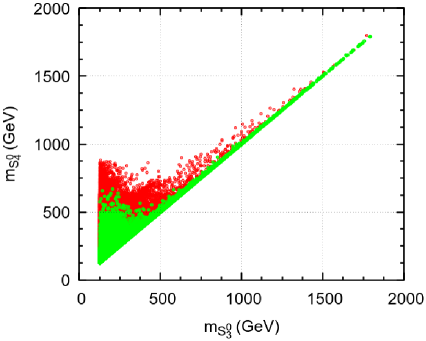
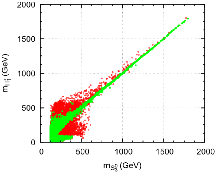
Figure 1: Left panel: Relation between $m_{S_{3}^{0}}$ and $m_{S_{4}^{0}}$. Right panel: Relation between $m_{S_{3}^{0}}$ and $m_{H_{1}^{+}}$. Color conventions: No cuts (red); with cuts (green)

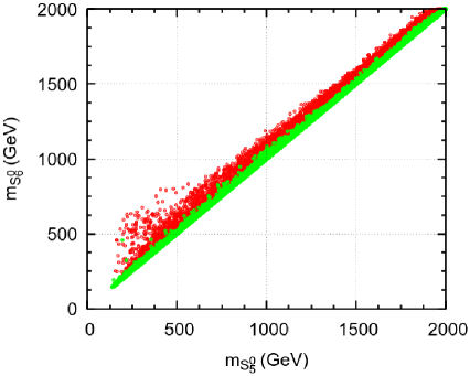
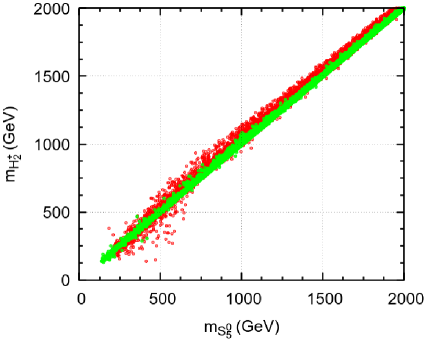
Figure 2: Left panel: Relation between $m_{S_{5}^{0}}$ and $m_{S_{6}^{0}}$. Right panel: Relation between $m_{S_{5}^{0}}$ and $m_{H_{2}^{+}}$. Color conventions: No cuts (red); with cuts (green)

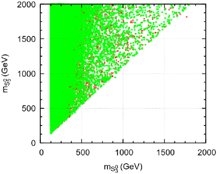
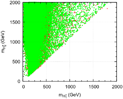
Figure 3: Left panel: Relation between $m_{S_{3}^{0}}$ and $m_{S_{5}^{0}}$. Right panel: Relation between $m_{H_{1}^{+}}$ and $m_{H_{2}^{+}}$. Color conventions: No cuts (red); with cuts (green)

7.3 The $\kappa_{V}$ constraint

We can now implement the $\kappa_{V}$ constraint on the model. In the following figures, in red are points without cuts, in green with cuts but no $\kappa_{V}$ constraint, and finally in blue points remaining after this constraint is applied. We took the ATLAS result of Eq. (69) at $2\sigma$. While the theoretical constraints cut around 88% of the points, the $\kappa_{V}$ constraint only cuts 22% of the remaining points. In Fig. 4 we show the relation between $\kappa_{V}$ and $\Lambda_{1,4}$ for the three sets of points as discussed above.

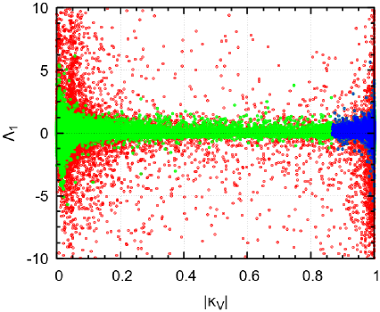
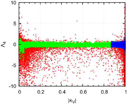
Figure 4: Left panel: Relation between $\kappa_{V}$ and $\Lambda_{1}$. Right panel: Relation between $\kappa_{V}$ and $\Lambda_{4}$. Color conventions: No cuts (red), with theoretical cuts (green), and after the $\kappa_{V}$ constraint (blue).

In fact it is not obvious from Fig. 4 that the $\kappa_{V}$ constraint only cuts about 22% of the points that pass the other cuts. This is because there is a very large number of points with $|\kappa_{V}|\lesssim 1$, even without theoretical cuts, and this is even more so after imposing the theoretical cuts. In this figure, we have 200000 points in the green region, but from these 156516 are in the blue region. That is, after theoretical cuts, 78% of the points also satisfy the $\kappa_{V}$ constraint. In Fig. 5 we show the relation between $\Lambda_{0}$ and $\Lambda_{3,4}$ for the same sets of points.

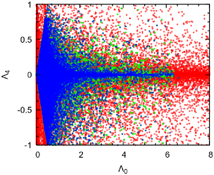
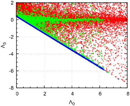
Figure 5: Left panel: Relation between $\Lambda_{0}$ and $\Lambda_{4}$. Right panel: Relation between $\Lambda_{0}$ and $\Lambda_{3}$ Color conventions: No cuts (red), with theoretical cuts (green), and after the $\kappa_{V}$ constraint (blue).

We see that, while for $(\Lambda_{0},\,\Lambda_{4})$ there is not much difference before and after the $\kappa_{V}$ constraint, the same is not true for $(\Lambda_{0},\,\Lambda_{3})$, where the constraints impose a linear relation between those two parameters. We note that, while $\Lambda_{0}$ is always positive, $\Lambda_{3}$ can be negative respecting the BFB condition in Eq. (58), $\Lambda_{0}+\Lambda_{3}\geq 0$, as it is clear in the right-handed panel of Fig. 5. Before we end this section, let us remark that we did not redraw the figures in Sec. 7.2 after imposing the $\kappa_{V}$ constraint, as the blue points would just superimpose the green points, as we have checked.

8 Conclusions

It is known that the 3HDM symmetric under an exact $A_{4}$ symmetry is not compatible with non-zero quark masses and/or non-block-diagonal CKM matrix [13]. In this work, we studied a 3HDM with $A_{4}$ softly broken. This allows us to evade the above result, by enlarging the structure of the possible vacua.

We obtained an excellent fit of the quarks mass matrices, including the CP-violating Jarlskog invariant. This leads to a unique solution for the vevs. We showed that, with the solution for the vevs obtained from the fit, it is possible to have a local minimum of the potential. We enforce this by imposing that all squared masses are positive. As in our scheme the scalar masses are not input parameters, we have to restrict one of the neutral scalars to have the mass of the known Higgs boson.

We have implemented the BFB, perturbative unitarity and the oblique parameters $S,T,U$ theoretical constraints. From LHC, we have considered the observed Higgs mass and the $\kappa_{V}$ constraint. After imposing the other constraints, we found that most of the points are close to the alignment required to respect the experimental $\kappa_{V}$ constraint. We have discovered a strong correlation among the masses of the scalars, even before applying the theoretical constraints, especially for moderate to large scalar masses.

One important point is that we have numerically checked for all the points that pass our constraints, that for a given set of parameters of the potential, our minimum is the true global minimum.

Acknowledgments

This work is supported in part by FCT (Fundação para a Ciência e Tecnologia) under Contracts CERN/FIS-PAR/0002/2021, CERN/FIS-PAR/0008/2019, UIDB/00777/2020, and UIDP/00777/2020; these projects are partially funded through POCTI (FEDER), COMPETE, QREN, and the EU. The work of I.B. was supported by a CFTP fellowship with reference BL210/2022-IST-ID and the work of S. C. by a CFTP fellowship with reference BL255/2022-IST-ID.

Appendix A The matrices $H_{d}$ and $H_{u}$

$$H_{d}(1,1)= \Sigma_{d}v^{2}\cos^{2}(\beta_{1})\cos^{2}(\beta_{2})$$ (75)

$$H_{d}(1,2)= v^{2}Z_{d}\cos(\beta_{1})\cos^{2}(\beta_{2})\cos(\rho_{2}-\phi_{d})\sin(\beta_{1})$$

$$-i\,v^{2}Z_{d}\cos(\beta_{1})\cos^{2}(\beta_{2})\sin(\beta_{1})\sin(\rho_{2}-\phi_{d})$$ (76)

$$H_{d}(1,3)= v^{2}Z_{d}\cos(\beta_{1})\cos(\beta_{2})\cos(\rho_{3}+\phi_{d})\sin(\beta_{2})$$

$$-i\,v^{2}Z_{d}\cos(\beta_{1})\cos(\beta_{2})\sin(\beta_{2})\sin(\rho_{3}+\phi_{d})$$ (77)

$$H_{d}(2,1)= (H_{d}(1,2))^{*}$$ (78)

$$H_{d}(2,2)= \Sigma_{d}v^{2}\cos^{2}(\beta_{2})\sin^{2}(\beta_{1})$$ (79)

$$H_{d}(2,3)= v^{2}Z_{d}\cos(\beta_{2})\cos(\rho_{2}-\rho_{3}+\phi_{d})\sin(\beta_{1})\sin(\beta_{2})$$

$$+i\,v^{2}Z_{d}\cos(\beta_{2})\sin(\beta_{1})\sin(\beta_{2})\sin(\rho_{2}-\rho_{3}+\phi_{d})$$ (80)

$$H_{d}(3,1)= (H_{d}(1,3))^{*}$$ (81)

$$H_{d}(3,2)= (H_{d}(2,3))^{*}$$ (82)

$$H_{d}(3,3)= \Sigma_{d}v^{2}\sin^{2}(\beta_{2})$$ (83)

$$H_{u}(1,1)= \Sigma_{u}v^{2}\cos^{2}(\beta_{1})\cos^{2}(\beta_{2})$$ (84)

$$H_{u}(1,2)= v^{2}Z_{u}\cos(\beta_{1})\cos^{2}(\beta_{2})\cos(\rho_{2}+\phi_{u})\sin(\beta_{1})$$

$$+i\,v^{2}Z_{u}\cos(\beta_{1})\cos^{2}(\beta_{2})\sin(\beta_{1})\sin(\rho_{2}+\phi_{u})$$ (85)

$$H_{u}(1,3)= v^{2}Z_{u}\cos(\beta_{1})\cos(\beta_{2})\cos(-\rho_{3}+\phi_{u})\sin(\beta_{2})$$

$$-i\,v^{2}Z_{u}\cos(\beta_{1})\cos(\beta_{2})\sin(\beta_{2})\sin(-\rho_{3}+\phi_{u})$$ (86)

$$H_{u}(2,1)= (H_{u}(1,2))^{*}$$ (87)

$$H_{u}(2,2)= \Sigma_{u}v^{2}\cos^{2}(\beta_{2})\sin^{2}(\beta_{1})$$ (88)

$$H_{u}(2,3)= v^{2}Z_{u}\cos(\beta_{2})\cos(-\rho_{2}+\rho_{3}+\phi_{u})\sin(\beta_{1})\sin(\beta_{2})$$

$$+i\,v^{2}Z_{u}\cos(\beta_{2})\sin(\beta_{1})\sin(\beta_{2})\sin(-\rho_{2}+\rho_{3}+\phi_{u})$$ (89)

$$H_{u}(3,1)= (H_{u}(1,3))^{*}$$ (90)

$$H_{u}(3,2)= (H_{u}(2,3))^{*}$$ (91)

$$H_{u}(3,3)= \Sigma_{u}v^{2}\sin^{2}(\beta_{2})$$ (92)

Appendix B The minimization conditions

$$m^{2}_{11}= -\frac{\sec(\rho_{2})\sec(\rho_{3})}{24v_{1}^{2}}\left[-12\text{Im}(m^{2}_{23})v_{2}v_{3}\sin(2(\rho_{2}-\rho_{3}))+\cos(\rho_{2}-\rho_{3})\left(4\Lambda_{0}v_{1}^{2}v^{2}\right.\right.$$

$$\hskip 28.45274pt\left.\left.+6\Lambda_{1}v_{1}^{2}v_{2}^{2}+6\Lambda_{1}v_{1}^{2}v_{3}^{2}+3\Lambda_{1}v_{2}^{2}v_{3}^{2}-3\Lambda_{2}v_{2}^{2}v_{3}^{2}+2\Lambda_{3}v_{1}^{2}\left(2v_{1}^{2}-v_{2}^{2}-v_{3}^{2}\right)\right)\right.$$

$$\hskip 28.45274pt\left.+4\Lambda_{0}v_{1}^{2}v_{2}^{2}\cos(\rho_{2}+\rho_{3})+4\Lambda_{0}v_{1}^{2}v_{3}^{2}\cos(\rho_{2}+\rho_{3})+4\Lambda_{0}v_{1}^{4}\cos(\rho_{2}+\rho_{3})\right.$$

$$\hskip 28.45274pt\left.+6\Lambda_{1}v_{1}^{2}v_{2}^{2}\cos(\rho_{2}+\rho_{3})+6\Lambda_{1}v_{1}^{2}v_{3}^{2}\cos(\rho_{2}+\rho_{3})-3\Lambda_{1}v_{2}^{2}v_{3}^{2}\cos(3(\rho_{2}-\rho_{3}))\right.$$

$$\hskip 28.45274pt\left.+3\Lambda_{2}v_{2}^{2}v_{3}^{2}\cos(3(\rho_{2}-\rho_{3}))-2\Lambda_{3}v_{1}^{2}v_{2}^{2}\cos(\rho_{2}+\rho_{3})-2\Lambda_{3}v_{1}^{2}v_{3}^{2}\cos(\rho_{2}+\rho_{3})\right.$$

$$\hskip 28.45274pt\left.+4\Lambda_{3}v_{1}^{4}\cos(\rho_{2}+\rho_{3})+3\Lambda_{4}v_{1}^{2}v_{2}^{2}\sin(\rho_{2}-\rho_{3})+3\Lambda_{4}v_{1}^{2}v_{2}^{2}\sin(\rho_{2}+\rho_{3})\right.$$

$$\hskip 28.45274pt\left.+3\Lambda_{4}v_{1}^{2}v_{3}^{2}\sin(\rho_{2}-\rho_{3})-3\Lambda_{4}v_{1}^{2}v_{3}^{2}\sin(\rho_{2}+\rho_{3})-3\Lambda_{4}v_{2}^{2}v_{3}^{2}\sin(\rho_{2}-\rho_{3})\right.$$

$$\hskip 28.45274pt\left.+3\Lambda_{4}v_{2}^{2}v_{3}^{2}\sin(3(\rho_{2}-\rho_{3}))-12\text{Re}(m^{2}_{23})v_{2}v_{3}\cos(2(\rho_{2}-\rho_{3}))\right.$$

$$\hskip 28.45274pt\left.+24\text{Re}(m^{2}_{13})v_{1}v_{3}\cos(\rho_{2})+24\text{Re}(m^{2}_{12})v_{1}v_{2}\cos(\rho_{3})+12\text{Re}(m^{2}_{23})v_{2}v_{3}\right]$$ (93)

$$m^{2}_{22}= -\frac{1}{12v_{2}}\Big{[}3\sec(\rho_{2})\left(-4\text{Im}(m^{2}_{23})v_{3}\sin(\rho_{3})+v_{2}v_{3}^{2}(\Lambda_{1}-\Lambda_{2})\cos(\rho_{2}-2\rho_{3})-\Lambda_{4}v_{2}v_{3}^{2}\sin(\rho_{2}-2\rho_{3})\right.$$

$$\hskip 28.45274pt\left.+4\text{Re}(m^{2}_{23})v_{3}\cos(\rho_{3})+4\text{Re}(m^{2}_{12})v_{1}\right)+v_{2}\left(4\Lambda_{0}v^{2}+6\Lambda_{1}v_{1}^{2}+3\Lambda_{1}v_{3}^{2}+3\Lambda_{2}v_{3}^{2}\right.$$

$$\hskip 28.45274pt\left.-2\Lambda_{3}v_{1}^{2}+4\Lambda_{3}v_{2}^{2}-2\Lambda_{3}v_{3}^{2}+3\Lambda_{4}v_{1}^{2}\tan(\rho_{2})\right)\Big{]}$$ (94)

$$m^{2}_{33}= -\frac{1}{12v_{3}}\Big{[}3\sec(\rho_{3})\left(4\text{Im}(m^{2}_{23})v_{2}\sin(\rho_{2})+v_{2}^{2}v_{3}(\Lambda_{1}-\Lambda_{2})\cos(2\rho_{2}-\rho_{3})-\Lambda_{4}v_{2}^{2}v_{3}\sin(2\rho_{2}-\rho_{3})\right.$$

$$\hskip 28.45274pt\left.+4\text{Re}(m^{2}_{23})v_{2}\cos(\rho_{2})+4\text{Re}(m^{2}_{13})v_{1}\right)+v_{3}\left(4\Lambda_{0}\left(v_{1}^{2}+v_{2}^{2}+v_{3}^{2}\right)+6\Lambda_{1}v_{1}^{2}+3\Lambda_{1}v_{2}^{2}\right.$$

$$\hskip 28.45274pt\left.+3\Lambda_{2}v_{2}^{2}-2\Lambda_{3}v_{1}^{2}-2\Lambda_{3}v_{2}^{2}+4\Lambda_{3}v_{3}^{2}-3\Lambda_{4}v_{1}^{2}\tan(\rho_{3})\right)\Big{]}$$ (95)

$$\text{Im}(m^{2}_{12})= \frac{1}{4v_{1}}\Big{[}\sec(\rho_{2})\left(4\text{Im}(m^{2}_{23})v_{3}\cos(\rho_{2}-\rho_{3})-\Lambda_{1}v_{2}v_{3}^{2}\sin(2(\rho_{2}-\rho_{3}))-\Lambda_{1}v_{1}^{2}v_{2}\sin(2\rho_{2})\right.$$

$$\hskip 14.22636pt\left.+\Lambda_{2}v_{2}v_{3}^{2}\sin(2(\rho_{2}-\rho_{3}))+\Lambda_{2}v_{1}^{2}v_{2}\sin(2\rho_{2})-\Lambda_{4}v_{2}v_{3}^{2}\cos(2(\rho_{2}-\rho_{3}))\right.$$

$$\hskip 14.22636pt\left.+\Lambda_{4}v_{1}^{2}v_{2}\cos(2\rho_{2})-4\text{Re}(m^{2}_{23})v_{3}\sin(\rho_{2}-\rho_{3})-4\text{Re}(m^{2}_{12})v_{1}\sin(\rho_{2})\right)\Big{]}$$ (96)

$$\text{Im}(m^{2}_{13})= -\frac{1}{4v_{1}}\Big{[}\sec(\rho_{3})\left(4\text{Im}(m^{2}_{23})v_{2}\cos(\rho_{2}-\rho_{3})-\Lambda_{1}v_{2}^{2}v_{3}\sin(2(\rho_{2}-\rho_{3}))+\Lambda_{1}v_{1}^{2}v_{3}\sin(2\rho_{3})\right.$$

$$\hskip 14.22636pt\left.+\Lambda_{2}v_{2}^{2}v_{3}\sin(2(\rho_{2}-\rho_{3}))-\Lambda_{2}v_{1}^{2}v_{3}\sin(2\rho_{3})-\Lambda_{4}v_{2}^{2}v_{3}\cos(2(\rho_{2}-\rho_{3}))\right.$$

$$\hskip 14.22636pt\left.+\Lambda_{4}v_{1}^{2}v_{3}\cos(2\rho_{3})-4\text{Re}(m^{2}_{23})v_{2}\sin(\rho_{2}-\rho_{3})+4\text{Re}(m^{2}_{13})v_{1}\sin(\rho_{3})\right)\Big{]}$$ (97)

References

- [1] ATLAS collaboration, Observation of a new particle in the search for the Standard Model Higgs boson with the ATLAS detector at the LHC, Phys. Lett. B 716 (2012) 1 [1207.7214].
- [2] CMS collaboration, Observation of a New Boson at a Mass of 125 GeV with the CMS Experiment at the LHC, Phys. Lett. B 716 (2012) 30 [1207.7235].
- [3] E. Ma and G. Rajasekaran, Softly broken a(4) symmetry for nearly degenerate neutrino masses, Phys. Rev. D64 (2001) 113012 [hep-ph/0106291].
- [4] E. Ma, Quark mass matrices in the a(4) model, Mod. Phys. Lett. A17 (2002) 627 [hep-ph/0203238].
- [5] E. Ma, H. Sawanaka and M. Tanimoto, Quark Masses and Mixing with A4 Family Symmetry, Phys. Lett. B 641 (2006) 301 [hep-ph/0606103].
- [6] E. Ma, Suitability of a(4) as a family symmetry in grand unification, Mod. Phys. Lett. A21 (2006) 2931 [hep-ph/0607190].
- [7] L. Lavoura and H. Kuhbock, A(4) model for the quark mass matrices, Eur. Phys. J. C 55 (2008) 303 [0711.0670].
- [8] S. Morisi and E. Peinado, An A4 model for lepton masses and mixings, Phys. Rev. D80 (2009) 113011 [0910.4389].
- [9] R. de Adelhart Toorop, F. Bazzocchi, L. Merlo and A. Paris, Constraining Flavour Symmetries At The EW Scale I: The A4 Higgs Potential, JHEP 03 (2011) 035 [erratum: JHEP 01 (2013) 098] [1012.1791].
- [10] A. Degee, I.P. Ivanov and V. Keus, Geometric minimization of highly symmetric potentials, JHEP 02 (2013) 125 [1211.4989].
- [11] M. Leurer, Y. Nir and N. Seiberg, Mass matrix models, Nucl. Phys. B 398 (1993) 319 [hep-ph/9212278].
- [12] R. González Felipe, I.P. Ivanov, C.C. Nishi, H. Serôdio and J.P. Silva, Constraining multi-Higgs flavour models, Eur. Phys. J. C 74 (2014) 2953 [1401.5807].
- [13] R. González Felipe, H. Serôdio and J.P. Silva, Models with three Higgs doublets in the triplet representations of or , Phys. Rev. D 87 (2013) 055010 [1302.0861].
- [14] M.P. Bento, J.C. Romão and J.P. Silva, Unitarity bounds for all symmetry-constrained 3HDMs, JHEP 08 (2022) 273 [2204.13130].
- [15] C. Jarlskog, Commutator of the Quark Mass Matrices in the Standard Electroweak Model and a Measure of Maximal Nonconservation, Phys. Rev. Lett. 55 (1985) 1039.
- [16] N. Razzaghi, S. M. M. Rasouli, P. Parada and P. Moniz, Two-Zero Textures Based on Symmetry and Unimodular Mixing Matrix, Symmetry 14 (2022) no.11, 2410 [2203.05753]
- [17] G.C. Branco and L. Lavoura, Rephasing Invariant Parametrization of the Quark Mixing Matrix, Phys. Lett. B 208 (1988) 123.
- [18] F. James and M. Roos, Minuit: A System for Function Minimization and Analysis of the Parameter Errors and Correlations, Comput. Phys. Commun. 10 (1975) 343.
- [19] Particle Data Group collaboration, Review of Particle Physics, PTEP 2022 (2022) 083C01.
- [20] W. Grimus, L. Lavoura, O.M. Ogreid and P. Osland, A Precision constraint on multi-Higgs-doublet models, J. Phys. G35 (2008) 075001 [0711.4022].
- [21] I.P. Ivanov and F. Vazão, Yet another lesson on the stability conditions in multi-Higgs potentials, JHEP 11 (2020) 104 [2006.00036].
- [22] N. Buskin and I.P. Ivanov, Bounded-from-below conditions for -symmetric 3HDM, J. Phys. A 54 (2021) 325401 [2104.11428].
- [23] F.S. Faro and I.P. Ivanov, Boundedness from below in the three-Higgs-doublet model, Phys. Rev. D 100 (2019) 035038 [1907.01963].
- [24] S. Carrôlo, J.C. Romão and J.P. Silva, Conditions for global minimum in the symmetric 3HDM, Eur. Phys. J. C 82 (2022) 749 [2207.02928].
- [25] R. Boto, J.C. Romão and J.P. Silva, Bounded from below conditions on a class of symmetry constrained 3HDM, Phys. Rev. D 106 (2022) 115010 [2208.01068].
- [26] S.L. Glashow and S. Weinberg, Natural Conservation Laws for Neutral Currents, Phys. Rev. D 15 (1977) 1958.
- [27] P.M. Ferreira, L. Lavoura and J.P. Silva, Renormalization-group constraints on Yukawa alignment in multi-Higgs-doublet models, Phys. Lett. B 688 (2010) 341 [1001.2561].
- [28] K. Yagyu, Higgs boson couplings in multi-doublet models with natural flavour conservation, Phys. Lett. B 763 (2016) 102 [1609.04590].
- [29] ATLAS collaboration, A detailed map of Higgs boson interactions by the ATLAS experiment ten years after the discovery, Nature 607 (2022) 52 [2207.00092].