Symmetric Kondo Lattice States in Doped Strained Twisted Bilayer Graphene

Abstract

We use the topological heavy fermion (THF) model Song and Bernevig (2022) and its Kondo Lattice (KL) formulation Hu et al. to study the possibility of a symmetric Kondo state in twisted bilayer graphene. Via a large-$N$ approximation, we find a symmetric Kondo state in the KL model at fillings $\nu=0,\pm 1,\pm 2$ where a KL model can be constructed Hu et al. . In the symmetric Kondo state, all symmetries are preserved and the local moments are Kondo screened by the conduction electrons. At the mean-field level of the THF model at $\nu=0,\pm 1,\pm 2,\pm 3$ we also find a similar symmetric state that is adiabatically connected to the symmetric Kondo state Coleman (2015). We study the stability of the symmetric state by comparing its energy with the ordered (symmetry-breaking) states found in Ref. Song and Bernevig (2022) and find the ordered states to have lower energy at $\nu=0,\pm 1,\pm 2$. However, moving away from integer fillings by doping holes to the light bands, our mean-field calculations find the energy difference between the ordered state and the symmetric state to be reduced, which suggests the loss of ordering and a tendency towards Kondo screening. We expect that including the Gutzwiller projection in our mean-field state will further reduce the energy of the symmetric state. In order to include many-body effects beyond the mean-field approximation, we also performed dynamical mean-field theory (DMFT) calculations on the THF model in the non-ordered phase. The spin susceptibility follows a Curie behavior at $\nu=0,\pm 1,\pm 2$ down to $\sim 2\text{K}$ where the onset of screening of the local moment becomes visible. This hints to very low Kondo temperatures at these fillings, in agreement with the outcome of our mean-field calculations. At non-integer filling $\nu=\pm 0.5,\pm 0.8,\pm 1.2$ DMFT shows deviations from a $1/T$-susceptibility at much higher temperatures, suggesting a more effective screening of local moments with doping. Finally, we study the effect of a $C_{3z}$-rotational-symmetry-breaking strain via mean-field approaches and find that a symmetric phase (that only breaks $C_{3z}$ symmetry) can be stabilized at sufficiently large strain at $\nu=0,\pm 1,\pm 2$. Our results suggest that a symmetric Kondo phase is strongly suppressed at integer fillings, but could be stabilized either at non-integer fillings or by applying strain.

Introduction— The experiments on magic-angle $(\theta=1.05^{\circ})$ twisted bilayer graphene (MATBLG) Bistritzer and MacDonald (2011); Balents et al. (2020a); Andrei et al. (2021) have established the existence of a variety of interesting phases Cao et al. (2020a); Lu et al. (2019); Stepanov et al. (2020); Xie and MacDonald (2021); Kerelsky et al. (2019); Jiang et al. (2019); Wong et al. (2020); Zondiner et al. (2020); Choi et al. (2021); Park et al. (2021); Lu et al. (2021); Saito et al. (2021a); Rozen et al. (2021); Das et al. (2022); Seifert et al. (2020); Otteneder et al. (2020); Lisi et al. (2021); Benschop et al. (2021); Hesp et al. (2021); Hubmann et al. (2022); Jaoui et al. (2022); Grover et al. (2022), including correlated insulating phases Cao et al. (2018a, 2020b); Polshyn et al. (2019); Liu et al. (2021a); Xie et al. (2019); Choi et al. (2019); Nuckolls et al. (2020); Saito et al. (2021b); Das et al. (2021); Wu et al. (2021); Stepanov et al. (2021) and superconductivity Cao et al. (2018b, 2021); Yankowitz et al. (2019); Diez-Merida et al. (2021); Di Battista et al. (2022). Their discovery has been followed by considerable theoretical efforts  Efimkin and MacDonald (2018); Vafek and Kang (2020); Padhi et al. (2018, 2020); Guinea and Walet (2018); Dodaro et al. (2018); Hejazi et al. (2021); Khalaf et al. (2021); Po et al. (2018); König et al. (2020); Christos et al. (2020); Kennes et al. (2018); Huang et al. (2020); Guo et al. (2018); Cha et al. (2021); Kang et al. (2021); Wu et al. (2019); Balents et al. (2020b); Fernandes and Venderbos (2020); Wilson et al. (2020); Cea et al. (2019); Yu et al. (2022); Herzog-Arbeitman et al. (2020, 2022); Yu et al. aimed at understanding their origin. An extended Hubbard model has been constructed to analyze the interacting physics Kang and Vafek (2019, 2018); Koshino et al. (2018); Ochi et al. (2018); Vafek and Kang (2021); Ochi et al. (2018); Xu and Balents (2018); Xu et al. (2018); Venderbos and Fernandes (2018); Yuan and Fu (2018); Da Liao et al. (2019, 2021); Chichinadze et al. (2020); Kang et al. (2021); Seo et al. (2019), however, due to the non-trivial topology of the flat bands  Liu et al. (2019a); Zou et al. (2018); Song et al. (2019); Po et al. (2019); Lian et al. (2020); Hejazi et al. (2019a); Liu et al. (2018); Thomson et al. (2018); Song et al. (2021), certain symmetries become non-local. Alternatively, an approach based on a momentum space model has been considered Bultinck et al. (2020a); Bernevig et al. (2021a); Xie et al. (2021); You and Vishwanath (2019); Wu and Das Sarma (2020); Isobe et al. (2018); Liu et al. (2019b); Wang et al. (2021); Bernevig et al. (2021b), in which correlated insulators Bultinck et al. (2020b); Lian et al. (2021); Bernevig et al. (2021c); Liu and Dai (2021); Cea and Guinea (2020); Zhang et al. (2020); Liu et al. (2021b); Xie and MacDonald (2020), superconductivity Lian et al. (2019); Wu et al. (2018); González and Stauber (2019); Lewandowski et al. (2021); Hejazi et al. (2019b); Xie et al. (2020), and other correlated quantum phases Kwan et al. (2021); Ledwith et al. (2020); Abouelkomsan et al. (2020); Repellin and Senthil (2020); Sheffer and Stern (2021) have been identified and studied. Besides, various numerical calculations Kang and Vafek (2020); Soejima et al. (2020); Eugenio and Dag (2020); Huang et al. (2019); Zhang et al. (2021); Hofmann et al. (2022); Repellin et al. (2020); Zhang et al. (2022) have also been performed to investigate the correlated nature of the phenomena. However, the active phase diagram including the states at non-integer fillings is not well understood. The exact mapping between the MATBLG and topological heavy-fermion model constructed in Ref. Song and Bernevig (2022) could be used for developments in this direction. This mapping establishes a bridge between heavy-fermions Hewson (1997); Coleman (2015); Stewart (1984); Si and Steglich (2010); Gegenwart et al. (2008) and moiré systems Song and Bernevig (2022); Hu et al. ; Ramires and Lado (2021). The presence of localized moments in MATBG is supported by recent entropy measurements which have found a Pomeranchuk-type transition Saito et al. (2020); Rozen et al. (2021). A large entropy observed at high-temperatures, originates from weakly interacting local moments whose fluctuations are quenched at low temperatures Saito et al. (2020); Rozen et al. (2021). Since a similar behavior is observed in heavy fermion systems Coleman (2015); Hewson (1997), where the fluctuating local moments are screened by conduction electrons (Kondo effect), this observation is suggestive of a Kondo state with screened local moments in MATBLG Hewson (1997); Lau and Coleman .

In this paper we use the KL model Hu et al. , to describe and study the symmetric Kondo (SK) state. We focus on integer fillings $\nu=0,\pm 1,\pm 2$, where a KL model can be constructed Hu et al. (a KL description fails at $\nu=\pm 3$ as demonstrated in Ref. Hu et al. ). The SK phase preserves all symmetries; the local moments are screened. We discuss the topology and the band structure of the SK state and extend the study to the THF model where we identify the symmetric state that is adiabatically connected to the SK state  Coleman (2015). In order to address integer and fractional fillings on equal footing, we perform both a mean-field and a dynamical mean-field theory (DMFT) calculations of the THF defining a “periodic Anderson model” with a momentum-dependent hybridization between the correlated $f$- and the dispersive $c$-electrons in the non-ordered state.

Our mean-field calculations indicate that the energy of the symmetric state is higher than that of the ordered (symmetry-breaking) states found in Ref. Song and Bernevig (2022) at integer filling. We thus conclude that ordered states are more energetically favored at integer fillings. DMFT supports this picture as we obtain a Curie behavior of the local spin susceptibility at integer fillings, down to very low temperatures $\sim 2$K, hinting to a very small Kondo scale (lower than $\sim 2$K). Together with the mean-field results we would then expect an ordered state to be favored at low temperatures for these fillings.

Turning to the effect of doping, instead, from our mean-field analysis, we find that the energy difference between the symmetric phase and the ordered phase can be sizeably reduced. Doping hence suppresses the ordering and enhances the Kondo screening. This conclusion is further supported by the DMFT results at non-integer fillings. Here, we find clear deviations from the Curie behavior in the entire range from 10K down to $\sim$1K. Even though it is computationally too demanding to go further down in temperature, we point out that our evidence of a clear-cut difference in the screening properties between integer and fractional fillings is reliable. DMFT treats indeed local quantum fluctuations exactly Georges et al. (1996) and hence takes into account the many-body processes that can potentially lead to the screening of local moments at any filling.

Since realistic samples have intrinsic strains, we finally study the effect of a $C_{3z}$-breaking strain on the symmetric phase. Our mean-field calculations show that the order is suppressed by the strain effect and a symmetric state can be stabilized at a sufficiently large strain at $\nu=0,\pm 1,\pm 2$.

In summary, we conclude that a symmetric Kondo phase is absent at integer fillings of MATBLG, but could in principle be stabilized either at non-integer fillings or by applying strain.

Topological Heavy Fermion model and the Kondo lattice model— The THF model Song and Bernevig (2022) contains two types of electrons: topological conduction $c$-electrons ($c_{\mathbf{k},a\eta s}$) and localized $f$-electrons ($f_{\mathbf{R},\alpha\eta s}$). The operator $c_{\mathbf{k},a\eta s}$ annihilates conduction $c$-electron with momentum $\mathbf{k}$, orbital $a\in\{1,2,3,4\}$, valley $\eta\in\{+,-\}$ and spin $s\in\{\uparrow,\downarrow\}$. At the $\Gamma_{M}$-point for each valley and each spin projection, $c$-electrons in the orbital $1$ and $2$ transform according to the $\Gamma_{3}$ irreducible representation (of magnetic space group $P6^{\prime}2^{\prime}2)$ Song and Bernevig (2022). The remaining $c$-electrons ($a=3,4$) at the same valley with the same spin projection transform in the $\Gamma_{1}\oplus\Gamma_{2}$ reducible representation (of magnetic space group $P6^{\prime}2^{\prime}2)$ Song and Bernevig (2022). We will call them $\Gamma_{3}$ $c$-electrons ($a=1,2$) and $\Gamma_{1}\oplus\Gamma_{2}$ $c$-electrons ($a=3,4$) respectively. $f_{\mathbf{R},\alpha\eta s}$ is the annihilation operator of the $f$-electron at the moiré unit cell $\mathbf{R}$ with orbital $\alpha\in\{1,2\}$, valley $\eta$ and spin $s$. The Hamiltonian of the THF model Song and Bernevig (2022); SM is

$${\hat{H}}_{THF}={\hat{H}}_{c}+{\hat{H}}_{fc}+{\hat{H}}_{U}+{\hat{H}}_{W}+{\hat{H}}_{V}+{\hat{H}}_{J}$$ (1)

where ${\hat{H}}_{c}$ describes the kinetic term of conduction electrons, ${\hat{H}}_{fc}$ describes the hybridization between $f$-$c$ electrons Song and Bernevig (2022); SM . The interactions include an on-site Hubbard interaction of $f$-electrons (${\hat{H}}_{U}$ with $U=57.95$meV), a repulsion between $f$- and $c$-electrons (${\hat{H}}_{W}$ with $W=48$meV), a Coulomb interaction between $c$-electrons (${\hat{H}}_{V}$ with $V(\mathbf{q}=0)/\Omega_{0}=48.33$meV and $\Omega_{0}$ the area of moiré unit cell), and a ferromagnetic exchange coupling between $f$-and $c$-electrons (${\hat{H}}_{J}$ with $J=16.38$meV) Song and Bernevig (2022); SM .

Based on the THF model Song and Bernevig (2022), a KL model of MATBLG has been constructed via a generalized Schrieffer–Wolff (SW) transformation as shown in Ref. Hu et al. . The KL model is described by the following Hamiltonian

$${\hat{H}}_{Kondo}={\hat{H}}_{c}+{\hat{H}}_{cc}+{\hat{H}}_{K}+{\hat{H}}_{J}\,.$$ (2)

where ${\hat{H}}_{c},{\hat{H}}_{J}$ come from the original THF model and ${\hat{H}}_{cc},{\hat{H}}_{K}$ emerge from the SW transformation. ${\hat{H}}_{cc}$ is the one-body scattering term of $\Gamma_{3}$ $c$-electrons with the form of

$${\hat{H}}_{cc}= \sum_{|\mathbf{k}|<\Lambda_{c}}\sum_{\begin{subarray}{c}a,a^{\prime}\in\{1,2\}\\ \eta,s\end{subarray}}e^{-|\mathbf{k}|^{2}\lambda^{2}}:c_{\mathbf{k},a\eta s}^{\dagger}c_{\mathbf{k},a^{\prime}\eta s}:\bigg{(}\frac{-1}{D_{\nu_{c},\nu_{f}}}$$

$$+\frac{-1}{D_{\nu_{c},\nu_{f}}}\bigg{)}\begin{bmatrix}\gamma^{2}/2&\gamma v_{\star}^{\prime}(\eta k_{x}-ik_{y})\\ \gamma v_{\star}^{\prime}(\eta k_{x}+ik_{y})&\gamma^{2}/2\end{bmatrix}_{a,a^{\prime}}\,.$$ (3)

$\lambda$ is the damping factor of the $f$-$c$ hybridization in the THF model. $\gamma,v_{\star}^{\prime}$ characterize the zeroth order and linear order $f$-$c$ hybridization of the THF model with $v_{\star}^{\prime}$ characterizing a $\mathbf{k}$-dependent hybridization matrix Song and Bernevig (2022); SM . $D_{1,\nu_{c},\nu_{f}}$ and $D_{2,\nu_{c},\nu_{f}}$ are defined as

$$D_{1,\nu_{c},\nu_{f}}=(U-W)\nu_{f}-\frac{U}{2}+(\frac{-V(0)}{\Omega_{0}}+W){\nu}_{c}$$

$$D_{2,\nu_{c},\nu_{f}}=(U-W)\nu_{f}+\frac{U}{2}+(\frac{-V(0)}{\Omega_{0}}+W){\nu}_{c}\,,$$ (4)

where $\nu_{f},\nu_{c}$ are the filling of $f$- and $c$-electrons determined from the calculations of the THF model at the zero-hybridization limit Hu et al. . We point out that in the single-orbital Kondo model, the one-body scattering term merely introduces a chemical potential shift Coleman (2015); Schrieffer and Wolff (1966) of the $c$-electrons and is usually omitted. However, in our model, ${\hat{H}}_{cc}$ cannot be ignored for two reasons. First, ${\hat{H}}_{cc}$ is $\mathbf{k}$-dependent and thus introduces additional kinetic energy to the conduction electrons. From Eq. S24, we observe the $\mathbf{k}$-dependency mainly comes from the linear $\mathbf{k}$ term that is proportional to $v_{\star}^{\prime}$ and can be traced back to the $\mathbf{k}$-dependency of the hybridization matrix in the THF model. Secondly, even if we drop the $v_{\star}^{\prime}$ term in Eq. S24 ($v_{\star}^{\prime}=0$ corresponding to the chiral limit Song and Bernevig (2022)), ${\hat{H}}_{cc}$ still produces an energy shift for the $\Gamma_{3}$ $c$-electrons. Thus ${\hat{H}}_{cc}$ leads to the energy splitting between $\Gamma_{3}$ and $\Gamma_{1}\oplus\Gamma_{2}$ $c$-electrons and cannot be simply treated as a shift of the chemical potential.

${\hat{H}}_{K}$ is the Kondo interaction between $f$- and $\Gamma_{3}$ $c$-electrons whose explicit form is given in Refs. SM ; Hu et al. . The Kondo interaction consists of two parts: the zeroth order Kondo interaction proportional to $\gamma^{2}/D_{\nu_{c},\nu_{f}}$ and the first order Kondo interaction proportional to $\gamma v_{\star}^{\prime}/D_{\nu_{c},\nu_{f}}$, where $D_{\nu_{c},\nu_{f}}^{-1}=-D_{1,\nu_{c},\nu_{f}}^{-1}+D_{2,\nu_{c},\nu_{f}}^{-1}$. The zeroth order Kondo interaction term describes the antiferromagnetic interaction between the $U(8)$ moments of the $f$- and the $\Gamma_{3}$ $c$-electrons and has a $U(8)$ symmetry. The linear-order Kondo interaction only has a flat $U(4)$ symmetry and is $\mathbf{k}$-dependent Song and Bernevig (2022); SM . ${\hat{H}}_{J}$ is the ferromagnetic exchange interaction between $\Gamma_{1}\oplus\Gamma_{2}$ $c$- and $f$-electrons that already exists in the TFH model Song and Bernevig (2022); SM . We also note that, for both the THF model and the KL model, ground states at filling $\nu$ and $-\nu$ are connected by a charge-conjugation transformation Song and Bernevig (2022). This can be broken by other one-body terms which we did not consider here. Therefore, in what follows, we only focus on $\nu\leq 0$.

Figure 1: (a) Band structure of the non-interaction THF model at $\nu=0$. (b), (c), (d) Band structure of the SK phase at $\nu=0,-1,-2$ respectively.

Mean-field Hamiltonian of the Kondo model— We next perform a mean-field study of the KL model Coleman (2015). This MF suppresses the RKKY interaction and essentially restores the hybridization term ${\hat{H}}_{fc}$ of the original periodic Anderson model, but in a renormalized form. It becomes exact in the $N\rightarrow\infty$ limit (we have $N=4$ here which corresponds to the approximate flat $U(4)$ symmetry of the KL Hamiltonian in Eq. 2). At the mean-field level, the Kondo interaction ${\hat{H}}_{K}$ can be written as (see Supplementary Materials (SM))

$${\hat{H}}_{K}^{MF}= \sum_{\mathbf{R},|\mathbf{k}|<\Lambda_{c}}\sum_{\alpha\eta s}\frac{e^{i\mathbf{k}\cdot\mathbf{R}-|\mathbf{k}|^{2}\lambda^{2}/2}}{\sqrt{N_{M}}D_{\nu_{c},\nu_{f}}}\Bigg{[}-f_{\mathbf{R},\alpha\eta s}^{\dagger}c_{\mathbf{k},a\eta s}$$

$$\begin{pmatrix}\gamma^{2}V_{1}^{*}+\gamma v_{\star}^{\prime}V_{2}^{*}&V_{1}^{*}(\eta k_{x}-ik_{y})\\ V_{1}^{*}(\eta k_{x}+ik_{y})&\gamma^{2}V_{1}^{*}+\gamma v_{\star}^{\prime}V_{2}^{*}\end{pmatrix}_{\alpha,a}+\text{h.c.}\bigg{]}$$

$$+N_{M}\bigg{[}\gamma^{2}|V_{1}^{*}|^{2}+\gamma v_{\star}^{\prime}(V_{1}^{*}V^{*}_{2}+V_{2}^{*}V^{*}_{1})\bigg{]}+\text{H.T.}$$ (5)

where we have introduced the following mean fields

$$V^{*}_{1}= \sum_{\mathbf{R},|\mathbf{k}|<\Lambda_{c}}\sum_{\alpha\eta s}\frac{e^{i\mathbf{k}\cdot\mathbf{R}-|\mathbf{k}|^{2}\lambda^{2}/2}}{\sqrt{N_{M}}N_{M}}\langle\Psi|f_{\mathbf{R},\alpha\eta s}^{\dagger}c_{\mathbf{k},\alpha\eta s}|\Psi\rangle$$

$$V^{*}_{2}= \sum_{\mathbf{R},|\mathbf{k}|<\Lambda_{c}}\sum_{\alpha a\eta s}\frac{e^{i\mathbf{k}\cdot\mathbf{R}-|\mathbf{k}|^{2}\lambda^{2}/2}}{\sqrt{N_{M}}N_{M}}(\eta k_{x}\sigma_{x}+k_{y}\sigma_{y})_{\alpha a}$$

$$\langle\Psi|f_{\mathbf{r},\alpha\eta s}^{\dagger}c_{\mathbf{k},\alpha\eta s}|\Psi\rangle$$ (6)

with $|\Psi\rangle$ being the mean-field ground state, and H.T. denotes the Hartree term ($\langle f^{\dagger}f\rangle,\langle c^{\dagger}c\rangle$) whose explicit formula is in the Supplementay Materials (SM) SM . Several points are in order. First, as we have mentioned above, the mean field restores the hybridization of the original Anderson model, but in a renormalized form. $V^{*}_{1},V^{*}_{2}$ describe the renormalized hybridization between the $f$- and $\Gamma_{3}$ $c$-electrons driven by the Kondo interactions between two types of electrons($f$ and $\Gamma_{3}$ $c$) Coleman (2015); Read and Newns (1983). Second, it is necessary to keep the Hartree contributions. In the canonical Kondo model, the Hartree term merely produces a chemical potential shift (in the case without symmetry breaking) and hence can be omitted. Here, Hartree contributions (see SM SM ) are $\mathbf{k}$-dependent because of the $\mathbf{k}$-dependency of the Kondo interactions, and thus contribute to the dispersion of the conduction $c$-electrons. Furthermore, since only $\Gamma_{3}$ $c$-electrons contribute to the Kondo interaction, the Hartree term also produces an energy splitting between the $\Gamma_{3}$ and the $\Gamma_{1}\oplus\Gamma_{2}$ $c$-electrons.

As for ${\hat{H}}_{J}$, we perform a similar mean-field decoupling

$${\hat{H}}_{J}^{MF}= J\sum_{\mathbf{R},|\mathbf{k}|<\Lambda_{c},\alpha\eta s}\frac{e^{i\mathbf{k}\cdot\mathbf{R}}}{\sqrt{N_{M}}}\bigg{(}V_{3}\delta_{1,\eta(-1)^{\alpha+1}}f_{\mathbf{R},\alpha\eta s}^{\dagger}c_{\mathbf{k},\alpha+2\eta s}$$

$$+V_{4}\delta_{-1,\eta(-1)^{\alpha+1}}\eta f_{\mathbf{R},\alpha\eta s}^{\dagger}c_{\mathbf{k},\alpha+2\eta s}+\text{h.c.}\bigg{)}$$

$$-JN_{M}\bigg{[}|V_{3}|^{2}+|V_{4}|^{2}\bigg{]}+\text{H.T.}$$ (7)

where we have introduced the following two mean-field averages that describe the $f$-$c$ hybridization:

$$V_{3}=\sum_{\mathbf{R},|\mathbf{k}|<\Lambda_{c}}\sum_{\alpha\eta,s}\frac{e^{i\mathbf{k}\cdot\mathbf{R}}\delta_{1,\eta(-1)^{\alpha+1}}}{\sqrt{N_{M}}N_{M}}\langle\Psi|f_{\mathbf{R},\alpha\eta s}^{\dagger}c_{\mathbf{k},\alpha+2\eta s}|\Psi\rangle$$

$$V_{4}=\sum_{\mathbf{R},|\mathbf{k}|<\Lambda_{c}}\sum_{\alpha\eta,s}\frac{e^{i\mathbf{k}\cdot\mathbf{R}}\delta_{-1,\eta(-1)^{\alpha+1}}}{\sqrt{N_{M}}N_{M}}\langle\Psi|\eta f_{\mathbf{R},\alpha\eta s}^{\dagger}c_{\mathbf{k},\alpha+2\eta s}|\Psi\rangle\,,$$ (8)

To impose the filling of the $f$-electrons to be $\nu_{f}$, we introduce the Lagrange multiplier  Lau and Coleman ; Read and Newns (1983); SM :

$${\hat{H}}_{\lambda_{f}}=\sum_{\mathbf{R},\alpha\eta s}\lambda_{f}\bigg{(}:f_{\mathbf{R},\alpha\eta s}^{\dagger}f_{\mathbf{R},\alpha\eta s}:-\nu_{f}\bigg{)}$$ (9)

with $\lambda_{f}$ to be determined self-consistently SM . Finally, we introduce a chemical potential $\mu_{c}$ to the $c$-electrons

$${\hat{H}}_{\mu_{c}}=-\mu_{c}\sum_{|\mathbf{k}|<\Lambda_{c},a\eta s}:c_{\mathbf{k},a\eta s}^{\dagger}c_{\mathbf{k},a\eta s}:\,.$$ (10)

In the calculation, we tune $\mu_{c}$ and $\lambda_{c}$ together to fix both the total filling $\nu=\nu_{f}+\nu_{c}$ and the filling of $f$-electrons SM . The final mean-field Hamiltonian of the KL model now is

$${\hat{H}}_{Kondo}^{MF}={\hat{H}}_{c}+{\hat{H}}_{cc}+{\hat{H}}_{K}^{MF}+{\hat{H}}_{J}^{MF}+{\hat{H}}_{\lambda_{f}}+{\hat{H}}_{\mu_{c}}\,.$$ (11)

We then self-consistently solve the mean-field equations (see SM SM ). At $\nu=\nu_{f}=0,-1,-2$ (where a KL model can be constructed), we identify a SK state that preserves all the symmetries and is characterized by $V^{*}_{1}\neq 0,V^{*}_{2}\neq 0,V^{*}_{3}=0,V^{*}_{4}=0$ SM . We comment that the exchange interaction ${\hat{H}}_{J}$ Song and Bernevig (2022) between $f$- and $\Gamma_{1}\oplus\Gamma_{2}$ $c$-electrons is ferromagnetic, and hence disfavors the singlet formation or hybridization ($V_{3},V_{4}$) between $f$- and $\Gamma_{1}\oplus\Gamma_{2}$ $c$-electrons. We find that $V_{3},V_{4}$ vanish (their numerical amplitudes are smaller than $10^{-5}$). In fact, ${\hat{H}}_{J}$ favors the triplet formation or pairing formation ($f^{\dagger}c^{\dagger}$), where both lead to a symmetry-breaking state at the mean-field level and are beyond our current consideration of SK state.

Properties of the symmetric Kondo phase— In Fig. 1, we plot the band structure of the SK phase and compare it with the non-interacting THF model. We find the hybridization in the SK state defined in Eq. 5 to be enhanced compared to the non-interacting limit of THF model, which is clear from the increase of the gap of the $\Gamma_{3}$ states at the $\Gamma$ point Song and Bernevig (2022) from its non-interacting value $24.75$meV at $\nu=0$, to $168$meV, $190$meV, $213$meV at $\nu=0,-1,-2$ respectively. We also find that in the SK phase the bandwidths of the flat bands at $\nu=-1,-2$ become $16$meV, $53$meV, which are (much) larger than the non-interacting flat-band bandwidth ($=7.4$meV) of the THF model (Fig. 1). However, at $\nu=0$, the flat-band bandwidth is the same as the non-interacting flat-band bandwidth. This is because, at $\nu=0$, the one-body scattering term and the Hartree contributions from ${\hat{H}}_{K},{\hat{H}}_{J}$ all vanish SM , and the enhanced hybridization pushes the remote bands away from the Fermi energy and does not change much the band structures of the flat bands. In addition, unlike the non-interacting case, here we found the flat bands are mostly formed by $\Gamma_{1}\oplus\Gamma_{2}$ $c$-electrons with orbital weights larger than $70\%$ at $\nu=0,-1,-2$. This is because the large $f$-$c$ hybridization induced by $V_{1},V_{2}$ (Eq. 5) pushes the energy of $\Gamma_{3}$ $c$- and $f$-electrons away from the Fermi energy and reduces their orbital weights SM .

The flat bands in the SK phase form $\Gamma_{1}\oplus\Gamma_{2}$, $M_{1}\oplus M_{2}$ and $K_{2}K_{3}$ representations at $\Gamma_{M},M_{M},K_{M}$ respectively, and have the same topology as the flat bands in the non-interacting THF model Song and Bernevig (2022). More explicitly, the flat bands for each valley and each spin projection belong to a fragile topology Song and Bernevig (2022) at $\nu=-1,-2$. At $\nu=0$, due to the additional particle-hole symmetry, flat bands have a stable topology Song and Bernevig (2022); Song et al. (2019, 2021); SM , which is characterized by the odd winding number of the Wilson loop as shown in supplementary material SM . We mention that the interplay between Kondo effect and the topological bands has also been studied in various other systems Dzero et al. (2010); Lai et al. (2018); Hu and Si (2022); Chen et al. (2022); Dzero et al. (2016); Lei et al. (2021).

Symmetric phase in the topological heavy-fermion model— We next investigate the similar symmetric phase in the THF model Eq. 1. We first focus on integer fillings $\nu=0,-1,-2,-3$ and perform the mean-field calculations of THF as introduced in Ref. Song and Bernevig (2022); SM . By enforcing the mean-field Hamiltonian to preserve all the symmetries, we are able to identify a symmetric state that preserves all the symmetries at $\nu=0,-1,-2,-3$. To observe the stability of the symmetric phase, we compare its energy ($E_{sym}$) with the energy ($E_{order}$) of the ordered (symmetry-breaking) ground states derived in Ref. Song and Bernevig (2022). The ordered ground states in Ref. Song and Bernevig (2022) are a Kramers inter-valley-coherent (KIVC) state at $\nu=0$, a KIVC+valley polarized (VP) state at $\nu=-1$, a KIVC state at $\nu=-2$ and a VP state at $\nu=-3$. We point out that at $\nu=-3$ other states with lower energy exist Xie et al. (2022). In our numerical calculations, we find $\Delta E=E_{sym}-E_{order}=47\mathrm{meV},40\mathrm{meV},33\mathrm{meV},23\mathrm{meV}$ at $\nu=0,-1,-2,-3$ respectively. In all integer filling cases, the symmetric states have higher energy, and the ground states cannot be the symmetric state, which is consistent with the previous calculations of Ref. Hu et al. ; Song and Bernevig (2022); Bernevig et al. (2021c). Note that our mean-field calculation does not include a Gutzwiller projection to fix the filling of $f$-electrons at each site, and hence we expect the energy of projected symmetric states will be lower. However, as we show later, after including the effect of local correlations via the DMFT approach, we confirm that the Kondo phase, which is adiabatically connected to the symmetric phase in the mean-field calculations, is strongly suppressed at integer fillings (down to temperatures $\sim 1$-$2$K). This further supports the development of ordering at integer fillings.

Figure 2: Doping dependence of the ground state energy difference $\Delta E=E_{sym}-E_{order}$ near integer fillings $\nu_{t}=0,-1,-2,-3$.

Effects of doping— We next investigate the effects of doping, first at the level of mean-field theory. We stick to a narrow region $\nu\in[\nu_{int}-0.5,\nu_{int}+0.5]$ near each integer filling $\nu_{int}=0,-1,-2,-3$ and compare the energies of the ordered states $E_{ord}$ and the symmetric states $E_{sym}$ in the THF model. To find the ordered state solutions, we first initialize the calculations with the mean-field solutions at integer filling $\nu_{int}$ and fill the mean-field bands up to current filling $\nu$. We then self-consistently solve the mean-field equations and calculate the energy of the resulting states. We obtain the symmetric-state solution in a similar manner but take the symmetric solution at $\nu_{int}$ as initialization and enforce the symmetry of the mean-field Hamiltonian during the calculations. Fig. 2 displays a plot of the difference of the ground state energies $\Delta E=E_{sym}-E_{order}$ as a function of doping $\Delta\nu=\nu-\nu_{int}$ near $\nu_{int}=0,-1,-2,-3$. We observe that hole doping at $\nu=0,-1,-2,-3$ and electron doping at $\nu=0$ decreases the $\Delta E$. Doping holes at $\nu=0,-1,-2,-3$ and doping electrons at $\nu=0$ to the ordered states is equivalent to doping the light (dispersive) bands which are mostly formed by conduction $c$-electrons. After doping, the conduction electrons will stay close to the Fermi energy, and then enhance the tendency towards the Kondo effect.

However, doping electrons at $\nu=-1,-2$ to the ordered states is equivalent to doping heavy (flat) bands which mostly come from the $f$-electrons. Because of the flatness of the band, we find the nature of the ordered states will change with doping (see SM  SM ). For example at $\nu=2$, the KIVC order is suppressed by the electron doping (see SM SM ). Thus, $\Delta E$ will be affected by both, changes of ordering and doping. However, a sizeable change of the order parameters is not observed for hole doping at $\nu=0,-1,-2,-3$ and also electron doping at $\nu=0$ (see SM SM ), because we are doping conduction $c$-electrons in both cases. We also point out the complexity of $\nu=-3$. First, other states that break translational invariant Xie et al. (2022) could have lower energy than the VP state we currently considered. Second, even for the VP state, doping electrons is equivalent to doping both heavy and light bands Song and Bernevig (2022), since both light and heavy bands appear in the electron doping case Song and Bernevig (2022). In practice, as we increase $\Delta\nu$, we find that, at $\nu=-1,-2$, $\Delta E$ will first decrease and then increase and, at $\nu=-3$, $\Delta E$ will always increase.

In summary, we conclude that hole doping can suppress the long-range order and enhance the tendency towards the Kondo effect near $\nu=0,-1,-2$. Electron doping, depending on the fillings, could also enhance the tendency toward the Kondo effect. However, on the electron doping side, the change of order moments indicates the importance of the correlation effect which could be underestimated in the mean-field approach. In the next section, we provide a more comprehensive study of the doping effect using the DMFT calculation.

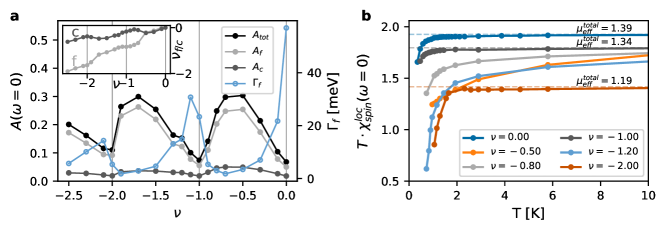
Figure 3: DMFT solution of the THF model. (a) Doping $\nu$ dependent low-energy spectral function at the Fermi level ($A(\omega=0)$) for the full system $A_{tot}$, the c- ($A_{c}$) and the f-electrons ($A_{f}$) at $11.6$ K. Also shown is the scattering rate $\Gamma_{f}$ as extracted from the local f-electron self-energy. (b) Effective local moment $T\cdot\chi_{\text{spin}}^{\text{loc}}(\omega=0)$ as a function of temperature $T$ for different doping levels $\nu$.

Dynamical mean-field theory results of the THF model—

In the following, we present the dynamical mean-field theory resultss of the THF model (Eq. 1), where we describe the local quantum many-body effects of the density-density Hubbard term ${\hat{H}}_{U}$ within the $f$-subspace. The ${\hat{H}}_{W}$ and ${\hat{H}}_{V}$ interactions involving density fluctuations on the $c$ orbitals are accounted for at the static mean-field level. We neglect ordered phases and perform calculations in the non-ordered one. There, we focus in particular on lifetime effects, quasiparticle weights and exploit the ability of DMFT to take local vertex corrections to the spin-spin correlation function into account.

First, DMFT finds a qualitative difference between the strong quasiparticle renormalization when the $f$+$c$ manifold is occupied with an integer number of electrons and a lighter Fermi liquid at fractional fillings: this can be seen from the scattering rate $\Gamma_{f}=-\text{Im}\Sigma_{f}(\omega=0)$ which is shown as a function of the total filling $\nu$ at $T=11.6$K (light blue empty circles) in Fig.3(a). The largest scattering rates are found close to $\nu=0.0$, -1.0 and -2.0, progressively decreasing as one moves away from the charge neutrality point. Correspondingly, the spectral weight at the Fermi level (black and grey solid circles) is suppressed at these fillings, with a residual nonzero value due to the finite temperature on the one hand and the resilient $f$/$c$ hybridization on the other.

Fig.3(b) illustrates the temperature-dependent screening of the local magnetic moment on the $f$ orbitals at different fillings. A flat $T\cdot\chi_{\text{spin}}^{\text{loc}}(\omega=0)$ indicates Curie behavior and a well-defined effective local moment, while deviations signal the onset of screening and a crossover towards a renormalized Pauli-like behavior, in agreement with the general expectation of zero-temperature Fermi-liquid in the periodic Anderson model de’ Medici et al. (2005). While at $\nu=0.0$, -1.0 and -2.0 the $1/T$ local spin susceptibility persists down to 1-2 K, the fractional fillings deviate from Curie at much higher temperatures, in line with the better Fermi-liquid nature signaled by the single-particle quantities in Fig.3(a).

As in the Hartree-Fock treatment of the THF model, DMFT confirms the difference between electron doping and hole doping (particle-hole asymmetry) near integer filling $\nu=-1$ and -2. Here, DMFT reveals particle-hole asymmetric scattering rates (Fig. 3(a)) and also in the difference of effective local moments at $\nu=-0.8$ and $-1.2$(Fig. 3(b)).

In summary, our DMFT calculations confirm that the Kondo phase is strongly suppressed at integer fillings $\nu=0,-1,-2$, increasing the propensity towards long-range order at these fillings. However, by doping the system, the development of Kondo screening (starting from $\sim 10$K) is observed, which suggests that doping could enhance the Kondo effect. This picture is consistent with our mean-field calculations.

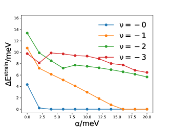
Figure 4: Energy difference $\Delta E^{strain}=E_{sym}^{strain}-E_{ord}^{strain}$ between the symmetric state that only breaks $C_{3z}$ symmetry ($E_{sym}^{strain}$) and the ordered state ($E_{ord}^{strain}$) as a function of $\alpha$ - a parameter characterizing the strain amplitude. We note that even at zero strain $\alpha=0$, a symmetric state that only breaks $C_{3z}$ symmetry has lower energy than the fully symmetric state. Thus $\Delta E^{strain}$ at $\alpha=0$ is smaller than the corresponding $\Delta E$ in Fig. 2.

Effects of strain— Since twisted bilayer graphene samples exhibit intrinsic strain Zhang et al. (2022) and the ordered states are disfavored by strain, we investigate the effect of strain on the symmetric state of THF model via mean-field approach. We focus on $\nu=0,-1,-2,-3$ and introduce the following Hamiltonian SM that qualitatively characterizes the effect of strain

$${\hat{H}}_{strain}=\alpha\sum_{\mathbf{R},\eta s}(f_{\mathbf{R},1\eta s}^{\dagger}f_{\mathbf{R},2\eta s}+\text{h.c.})$$

where $\alpha$ is proportional to the strain amplitude (we leave the construction of a realistic strain Hamiltonian Nakatsuji and Koshino (2022a, b); Vafek and Kang (2022) for a future study). A non-zero $\alpha$ breaks the $C_{3z}$ symmetry but preserves all other symmetries SM . We compare the ground state energies of the symmetric states ($E^{strain}_{sym}$) and the ordered states ($E^{strain}_{ord}$) at non-zero strain. To obtain the symmetric state solution, we solve the mean-field equations by requiring the mean-field Hamiltonian to satisfy all symmetries except for the $C_{3z}$. We obtain the solution of the ordered states by initializing the mean-field calculations with the ordered ground states at zero strain and then perform self-consistent calculations. In Fig. 4, we plot the difference between the ground state energies of the symmetric and the ordered states $\Delta E^{strain}=E_{sym}^{strain}-E^{strain}_{order}$ as a function of the effective strain amplitude $\alpha$ with $0\text{meV}<\alpha<20$meV at $\nu=0,-1,-2,-3$. We observe that $\Delta E$ at $\nu=0,-1$ vanishes at sufficiently large strain. A detailed analysis SM of the wavefunction shows that the ordered state cannot be stabilized and converged to a $C_{3z}$ broken symmetric solution at large strain. By further increasing strain, we find a symmetric state at $\nu=-2$ can also be stabilized at $\alpha\sim 45$meV (see SM SM ). We conclude that a symmetric phase can be stabilized by sufficiently large strain at $\nu=0,-1,-2$. As for $\nu=-3$, we mention that other ordered states, that break translational symmetry and have lower energy than the VP state, exist even at zero strain. We leave a systematical analysis of $\nu=-3$ for future study. Finally, we comment that even at zero strain, a symmetric state that breaks $C_{3z}$ symmetry has lower energy than the fully symmetric state that preserves all the symmetries (including $C_{3z}$). Therefore, $\Delta E^{strain}$ (energy difference between a symmetric state that only breaks $C_{3z}$ and an ordered state) at zero strain $\alpha=0$ in Fig. 4 is smaller than the corresponding $\Delta E$ (energy difference between a fully symmetric state and an ordered state) in Fig. 2.

Discussion and summary— Our main result is that an ordered state, instead of a SK state, will be the ground state of the system at integer filling $\nu=0,-1,-2,-3$. Our mean-field calculations of THF model indicate ground state energy of the symmetric state is higher than the one of the ordered states at these fillings. Via DMFT calculations, we find the Kondo temperature to be substantially smaller than 2K. Thus, we conclude the Kondo effect is suppressed at integer filling $\nu=0,-1,-2,-3$, and the ground state is likely to be an ordered state. However, our mean-field calculations suggest doping can reduce the energy difference between the symmetric state and the ordered state enhancing the tendency towards the SK state. This has also been confirmed by the DMFT calculations which show a strong deviation from the Curie Weiss law at non-integer fillings $\nu=-0.5,-0.8,-1.2$ already around 10K. Furthermore, we show that a sufficiently large $C_{3z}$ breaking strain could also stabilize a symmetric state that only breaks the $C_{3z}$ symmetry at $\nu=0,-1,-2$. Therefore, we conclude both doping and strain enhance the Kondo effect and could, in principle, stabilize a SK state. Our results may explain the recent entropy experiments Saito et al. (2021a); Rozen et al. (2021) which reveal a high-temperature phase with fluctuating moments and a low-temperature Fermi liquid phase with unpolarized isospins. This could be understood as a sign of screening of the local moments and the development of the SK phase at low temperatures.

As far as the SK state is concerned, we have performed a systematic study of its band structure and topology. Via the mean-field approach, we successfully identified the SK state in the KL model, and a symmetric state, that is adiabatically connected to the SK state, in the THF model. For the SK state in the KL model, we find that the $\Gamma_{3}$ states near the $\Gamma_{M}$ point have been pushed away, and the bandwidth of the flat bands is enlarged at $\nu=-1,-2$. The hybridization between $f$-electrons and $\Gamma_{3}$ $c$-electons is enhanced by the Kondo interactions. Consequently, the flat bands are mostly formed by $\Gamma_{1}\oplus\Gamma_{2}$ $c$-electrons. The topology of the flat bands remains the same as in the non-interacting case. However, for the symmetric state in the THF model, the enhanced $f$-$c$ hybridization does not appear. We mention that the mean-field solution of the symmetric state in the THF model underestimates the correlation effect, which could be the origin of the weak $f$-$c$ hybridization. We expect introducing a Gutzwiller projector will give a more precise description of the symmetric state in the THF model.

Note added— After finishing this work, we learned that related, but not identical, results have also recently been obtained by the S. Das Sarma’s  Chou and Sarma (2022), P. Coleman’s Lau and Coleman , and Z. Song’s groups Zhou and Song . We also mention that results from Z. Song’s group are compatible with our DMFT results.

Acknowledgements— B. A. B.’s work was primarily supported by the DOE Grant No. DE-SC0016239, the Simons Investigator Grant No. 404513. H. H. was supported by the European Research Council (ERC) under the European Union’s Horizon 2020 research and innovation program (Grant Agreement No. 101020833). J. H. A. was supported by a Hertz Fellowship. D. C. was supported by the DOE Grant No. DE-SC0016239 and the Simons Investigator Grant No. 404513. A. M. T. was supported by the Office of Basic Energy Sciences, Material Sciences and Engineering Division, U.S. Department of Energy (DOE) under Contract No. DE-SC0012704. G. R, L. K, T. W., G. S. and R. V. thank the Deutsche Forschungsgemeinschaft (DFG, German Research Foundation) for funding through QUAST FOR 5249-449872909 (Projects P4 and P5). G.R. acknowledges funding from the European Commission via the Graphene Flagship Core Project 3 (grant agreement ID: 881603). T.W. acknowledges support by the Cluster of Excellence “CUI: Advanced Imaging of Matter” of the Deutsche Forschungsgemeinschaft (DFG)–EXC 2056–Project ID No. 390715994.

Supplementary Materials

S1 Toplogical heavy-fermion model

The topological heavy-fermion (THF) model introduced in Ref. Song and Bernevig (2022) takes the following Hamiltonian

$${\hat{H}}={\hat{H}}_{c}+{\hat{H}}_{fc}+{\hat{H}}_{U}+{\hat{H}}_{J}+{\hat{H}}_{W}+{\hat{H}}_{V}+{\hat{H}}_{\mu}$$ (S12)

The single-particle Hamiltonian of conduction $c$-electrons has the form of

$$\hat{H}_{c}=\sum_{\eta,s,a,a^{\prime},|\mathbf{k}|<\Lambda_{c}}H_{a,a^{\prime}}^{(c,\eta)}(\mathbf{k})c_{\mathbf{k}a\eta s}^{\dagger}c_{\mathbf{k}a^{\prime}\eta s}\quad,\quad H^{(c,\eta)}(\mathbf{k})=\begin{bmatrix}0_{2\times 2}&v_{\star}(\eta k_{x}\sigma_{0}+ik_{y}\sigma_{z})\\ v_{\star}(\eta k_{x}\sigma_{0}-ik_{y}\sigma_{z})&M\sigma_{x}.\end{bmatrix}$$ (S13)

where $\sigma_{0,x,y,z}$ are identity and Pauli matrices. $c_{\mathbf{k}a\eta s}$ represents the annihilation operator of the $a(=1,2,3,4)$-th conduction band basis of the valley $\eta(=\pm)$ and spin $s(=\uparrow,\downarrow)$ at the moiré momentum $\mathbf{k}$. At $\Gamma_{M}$ point ($\mathbf{k}=0$) of the moiré Brillouin zone (MBZ), $c_{\mathbf{k}1\eta s},c_{\mathbf{k}2\eta s}$ form a $\Gamma_{3}$ irreducible representation (of $P6^{\prime}2^{\prime}2$ group), $c_{\mathbf{k}3\eta s},c_{\mathbf{k}4\eta s}$ form a $\Gamma_{1}\oplus\Gamma_{2}$ reducible (into $\Gamma_{1}$ and $\Gamma_{2}$ - as they are written, the $c_{\mathbf{k}3\eta s},c_{\mathbf{k}4\eta s}$ are just the $\sigma_{x}$ linear combinations of $\Gamma_{1}\pm\Gamma_{2}$ ) representation (of $P6^{\prime}2^{\prime}2$ group). $\Lambda_{c}$ is the momentum cutoff for the $c$-electrons. $N$ is the total number of moiré unit cells. The parameter values are $v_{\star}=-4.303\mathrm{eV}\cdot\mathrm{\mathring{A}}$, $M=3.697$meV.

The hybridization between $f$ and $c$ electrons has the form of

$$\hat{H}_{fc}=\frac{1}{\sqrt{N_{M}}}\sum_{\begin{subarray}{c}|\mathbf{k}|<\Lambda_{c}\\ \mathbf{R}\end{subarray}}\sum_{\alpha a\eta s}\bigg{(}e^{i\mathbf{k}\cdot\mathbf{R}-\frac{|\mathbf{k}|^{2}\lambda^{2}}{2}}H^{(fc,\eta)}_{\alpha a}(\mathbf{k})f_{\mathbf{R}\alpha\eta s}^{\dagger}c_{\mathbf{k}a\eta s}+h.c.\bigg{)}\ ,$$ (S14)

where $f_{\mathbf{R}\alpha\eta s}$ represents the annihilation operators of the $f$ electrons with orbital index $\alpha(=1,2)$, valley index $\eta(=\pm)$ and spin $s(=\uparrow,\downarrow)$ at the moiré unit cell $\mathbf{R}$. $N_{M}$ is the number of moiré unit cells and $\lambda=0.3376a_{M}$ is the damping factor, where $a_{M}$ is the moiré lattice constant. The hybridization matrix $H^{(fc,\eta)}$ has the form of

$$H^{(fc,\eta)}(\mathbf{k})=\begin{pmatrix}\gamma\sigma_{0}+v_{\star}^{\prime}(\eta k_{x}\sigma_{x}+k_{y}\sigma_{y}),&0_{2\times 2}\end{pmatrix}$$ (S15)

which describe the hybridization between $f$ electrons and $\Gamma_{3}$ $c$ electrons $(a=1,2)$. The parameter values are $\gamma=-24.75$meV, $v_{\star}^{\prime}=1.622\mathrm{eV}\cdot\mathrm{\mathring{A}}$.

${\hat{H}}_{U}$ ($U=57.89\mathrm{meV}$) describes the on-site interactions of $f$-electrons.

$${\hat{H}}_{U}=\frac{U}{2}\sum_{\mathbf{R}}:n^{f}_{\mathbf{R}}::n^{f}_{\mathbf{R}}:,$$ (S16)

where $n^{f}_{\mathbf{R}}=\sum_{\alpha\eta s}f_{\mathbf{R}\alpha\eta s}^{\dagger}f_{\mathbf{R}\alpha\eta s}$ is the $f$-electrons density and the colon symbols represent the normal ordered operator with respect to the normal state: $:f^{\dagger}_{\mathbf{R}\alpha_{1}\eta_{1}s_{1}}f_{\mathbf{R}\alpha_{2}\eta_{2}s_{2}}:=f^{\dagger}_{\mathbf{R}\alpha_{1}\eta_{1}s_{1}}f_{\mathbf{R}\alpha_{2}\eta_{2}s_{2}}-\frac{1}{2}\delta_{\alpha_{1}\eta_{1}s_{1};\alpha_{2}\eta_{2}s_{2}}$.

The ferromagnetic exchange interaction between $f$ and $c$ electrons ${\hat{H}}_{J}$ is defined as

$$H_{J}=-\frac{J}{2N_{M}}\sum_{\mathbf{R}s_{1}s_{2}}\sum_{\alpha\alpha^{\prime}\eta\eta^{\prime}}\sum_{|\mathbf{k}_{1}|,|\mathbf{k}_{2}|<\Lambda_{c}}e^{i(\mathbf{k}_{1}-\mathbf{k}_{2})\cdot\mathbf{R}}(\eta\eta^{\prime}+(-1)^{\alpha+\alpha^{\prime}}):f_{\mathbf{R}\alpha\eta s_{1}}^{\dagger}f_{\mathbf{R}\alpha^{\prime}\eta^{\prime}s_{2}}::c_{\mathbf{k}_{2},\alpha^{\prime}+2,\eta^{\prime}s_{2}}^{\dagger}c_{\mathbf{k}_{1},\alpha+2,\eta s_{1}}:$$ (S17)

where $J=16.38$meV and $:c_{\mathbf{k}_{2},\alpha^{\prime}+2,\eta^{\prime}s_{2}}^{\dagger}c_{\mathbf{k}_{1},\alpha+2,\eta s_{1}}:=c_{\mathbf{k}_{2},\alpha^{\prime}+2,\eta^{\prime}s_{2}}^{\dagger}c_{\mathbf{k}_{1},\alpha+2,\eta s_{1}}-\frac{1}{2}\delta_{\mathbf{k}_{1},\mathbf{k}_{2}}\delta_{\alpha,\alpha^{\prime}}\delta_{\eta,\eta^{\prime}}\delta_{s_{1},s_{2}}$

The repulsion between $f$ and $c$ electrons ${\hat{H}}_{W}$ has the form of

$$\hat{H}_{W}=\sum_{\eta,s,\eta^{\prime},s^{\prime},a,\alpha}\sum_{|\mathbf{k}|<\Lambda_{c},|\bm{\mathbf{k}+\mathbf{q}}|<\Lambda_{c}}W_{a}e^{-i\mathbf{q}\cdot\mathbf{R}}:f_{\mathbf{R},a\eta s}^{\dagger}f_{\mathbf{R},a\eta s}::c_{\mathbf{k}+\mathbf{q},a\eta^{\prime}s^{\prime}}^{\dagger}c_{\mathbf{k},a\eta^{\prime}s^{\prime}}:$$ (S18)

where we take $W_{1}=W_{2}=44.03$meV and $W_{3}=W_{4}=50.20$meV.

The Coulomb interaction between $c$ electrons has the form of

$${\hat{H}}_{V}=\frac{1}{2\Omega_{0}N}\sum_{\eta_{1}s_{1}a_{1}}\sum_{\eta_{2}s_{2}a_{2}}\sum_{|\mathbf{k}_{1}|,|\mathbf{k}_{2}|<\Lambda_{c}}\sum_{\begin{subarray}{c}\mathbf{q}\\ |\mathbf{k}_{1}+\mathbf{q}|,|\mathbf{k}_{2}+\mathbf{q}|<\Lambda_{c}\end{subarray}}V(\mathbf{q}):c_{\mathbf{k}_{1}a_{1}\eta_{1}s_{1}}^{\dagger}c_{\mathbf{k}_{1}+\mathbf{q}a_{1}\eta_{1}s_{1}}::c_{\mathbf{k}_{2}+\mathbf{q}a_{2}\eta_{2}s_{2}}^{\dagger}c_{\mathbf{k}_{2}a_{2}\eta_{2}s_{2}}:$$ (S19)

where $\Omega_{0}$ is the area of the moiré unit cell and $V(\mathbf{q}=0)/\Omega_{0}=48.33\mathrm{meV}$. We will always treat ${\hat{H}}_{V}$ at mean-field level (int both the THF model and the Kondo lattice (KL) model) Song and Bernevig (2022)

$${\hat{H}}_{V}\approx\frac{V(0)}{\Omega_{0}}\nu_{c}\sum_{|\mathbf{k}|<\Lambda_{c},a,\eta,s}c_{\mathbf{k},a\eta s}^{\dagger}c_{\mathbf{k},a\eta s}-\frac{V(0)}{2\Omega_{0}}N_{M}\nu_{c}^{2}+\frac{V(0)}{\Omega_{0}}\sum_{|\mathbf{k}|<\Lambda_{c}}8\nu_{c}$$ (S20)

where $\nu_{c}$ is the filling of $c$ electrons $\nu_{c}=\frac{1}{N_{M}}\sum_{|\mathbf{k}|<\Lambda_{c},a,\eta,s}\langle\Psi|:c_{\mathbf{k},a\eta s}^{\dagger}c_{\mathbf{k},a\eta s}:|\Psi\rangle$ with $|\psi\rangle$ the ground state.

Finally, we introduce a chemical potential term

$${\hat{H}}_{\mu}=-\mu\sum_{|\mathbf{k}|<\Lambda_{c},a\eta s}c_{\mathbf{k},a\eta s}^{\dagger}c_{\mathbf{k},a\eta s}-\mu\sum_{\mathbf{R},\alpha\eta s}f_{\mathbf{R},\alpha\eta s}^{\dagger}f_{\mathbf{R},\alpha\eta s}\,.$$ (S21)

S2 Kondo lattice model

The Kondo lattice model is derived by performing a generalized Schrieffer-Wolff (SW) transformation on the topological heavy fermion model (detailed derivation in Ref. Hu et al. ). The Hamiltonian has the form of

$${\hat{H}}_{Kondo}={\hat{H}}_{c}+{\hat{H}}_{V}+{\hat{H}}_{W}+{\hat{H}}_{J}+{\hat{H}}_{K}+{\hat{H}}_{cc}-{\hat{H}}_{\mu_{c}}$$ (S22)

where ${\hat{H}}_{c}$ (Eq. S13), ${\hat{H}}_{V}$ (Eq. S19) and ${\hat{H}}_{W}$ (Eq. S18) and ${\hat{H}}_{J}$ (Eq. S17) come from the original TFH model. The Kondo interactions and the one-body scattering term are

$${\hat{H}}_{K}= \sum_{\mathbf{R},|\mathbf{k}|<\Lambda_{c},|\mathbf{k}^{\prime}|<\Lambda_{c}}\sum_{\alpha,\alpha^{\prime},a,a^{\prime},\eta,\eta^{\prime},s,s^{\prime}}\frac{e^{i(\mathbf{k}-\mathbf{k}^{\prime})\mathbf{R}-|\mathbf{k}|^{2}\lambda^{2}/2-|\mathbf{k}^{\prime}|^{2}\lambda^{2}/2}}{N_{M}D_{\nu_{c},\nu_{f}}}:f_{\mathbf{R},\alpha\eta s}^{\dagger}f_{\mathbf{R},\alpha^{\prime}\eta^{\prime}s^{\prime}}::c_{\mathbf{k}^{\prime},a^{\prime}\eta^{\prime}s^{\prime}}^{\dagger}c_{\mathbf{k},a\eta s}:$$

$$\bigg{[}\gamma^{2}\delta_{\alpha^{\prime},a^{\prime}}\delta_{\alpha,a}+\gamma v_{\star}^{\prime}\delta_{\alpha,a}[\eta^{\prime}k^{\prime}_{x}\sigma_{x}-k^{\prime}_{y}\sigma_{y}]_{\alpha^{\prime}a^{\prime}}+\gamma v_{\star}^{\prime}\delta_{\alpha^{\prime},a^{\prime}}[\eta k_{x}\sigma_{x}+k_{y}\sigma_{y}]_{\alpha a}\bigg{]}$$

and

$${\hat{H}}_{cc}= -\sum_{|\mathbf{k}|<\Lambda_{c},\eta,s}\sum_{a,a^{\prime}\in\{1,2\}}e^{-|\mathbf{k}|^{2}\lambda^{2}}\bigg{(}\frac{1}{D_{1,\nu_{c},\nu_{f}}}+\frac{1}{D_{2,\nu_{c},\nu_{f}}}\bigg{)}\begin{bmatrix}\gamma^{2}/2&\gamma v_{\star}^{\prime}(\eta k_{x}-ik_{y})\\ \gamma v_{\star}^{\prime}(\eta k_{x}+ik_{y})&\gamma^{2}/2\end{bmatrix}_{a,a^{\prime}}:c_{\mathbf{k},a\eta s}^{\dagger}c_{\mathbf{k},a^{\prime}\eta s}:$$ (S24)

where

$$D_{1,\nu_{c},\nu_{f}}=(U-W)\nu_{f}-\frac{U}{2}+(\frac{-V_{0}}{\Omega_{0}}+W){\nu}_{c}\quad,\quad D_{2,\nu_{c},\nu_{f}}=(U-W)\nu_{f}+\frac{U}{2}+(\frac{-V_{0}}{\Omega_{0}}+W){\nu}_{c}$$

$$D_{\nu_{c},\nu_{f}}=\bigg{[}-\frac{1}{D_{1,\nu_{c},\nu_{f}}}+\frac{1}{D_{2,\nu_{c},\nu_{f}}}\bigg{]}^{-1}\,.$$ (S25)

We point out that, at $\nu=\nu_{f}=\nu_{c}=0$, $D_{1,\nu_{c},\nu_{f}}=-D_{2,\nu_{c},\nu_{f}}$ and the on-body term ${\hat{H}}_{cc}(=0)$ vanishes.

We note that in the Kondo model the filling of $f$ electron at each site is fixed to be $\nu_{f}$. Then we can replace $\sum_{\alpha\eta s}:f_{\mathbf{R},\alpha\eta s}^{\dagger}f_{\mathbf{R},\alpha\eta s}:$ with $\nu_{f}$ and ${\hat{H}}_{W}$ becomes

$${\hat{H}}_{W}=\sum_{|\mathbf{k}|<\Lambda_{c},|\mathbf{k}^{\prime}|<\Lambda_{c},a\eta s}\sum_{\mathbf{Q}}W\nu_{f}:c_{\mathbf{k},a\eta^{\prime}s^{\prime}}^{\dagger}c_{\mathbf{k}^{\prime},a\eta s}\delta_{\mathbf{k},\mathbf{k}^{\prime}+\mathbf{Q}}$$ (S26)

where $\mathbf{Q}\in\{m\bm{b}_{M1}+m\bm{b}_{M2}|m,n\in\mathbb{Z}\}$ and $\mathbf{b}_{M1}$, $\mathbf{b}_{M2}$ are the reciprocal lattice vectors. If we focus on the conduction electrons within the first MBZ, we can replace $\delta_{\mathbf{k},\mathbf{k}^{\prime}+\mathbf{Q}}$ by $\delta_{\mathbf{k},\mathbf{k}^{\prime}}$ and

$${\hat{H}}_{W}=\sum_{|\mathbf{k}|<\Lambda_{c},a\eta s}\sum_{\mathbf{Q}}W\nu_{f}:c_{\mathbf{k},a\eta^{\prime}s^{\prime}}^{\dagger}c_{\mathbf{k},a\eta s}$$ (S27)

which is a chemical shift of conduction electrons. We also set $W_{1}=W_{2}=W_{3}=W_{4}=W=47.12$meV in ${\hat{H}}_{W}$ to simplify the SW transformation. The realistic values of $W_{1,2,3,4}$ are not identical but the difference is about $15\%$.

Finally, we introduce a chemical potential $\mu_{c}$ to tune the filling of the system

$${\hat{H}}_{\mu_{c}}=-\mu_{c}\sum_{|\mathbf{k}|<\Lambda_{c},a\eta s}:c_{\mathbf{k},a\eta s}^{\dagger}c_{\mathbf{k},a\eta s}:$$ (S28)

S3 Symmetry

We now provide the symmetry transformation of electron operators. For a given symmetry operation $g$, we let $D^{f}(g),D^{c^{\prime}}(g),D^{c^{\prime\prime}}(g)$ denote the representation matrix of $f$-, $\Gamma_{3}$ $c$- and $\Gamma_{1}\oplus\Gamma_{2}$ $c$-electrons:

$$gf_{\mathbf{R},\alpha\eta s}^{\dagger}g^{-1}=\sum_{\alpha^{\prime}\eta^{\prime}s^{\prime}}f_{g\mathbf{R},\alpha^{\prime}\eta^{\prime}s^{\prime}}^{\dagger}D^{f}(g)_{\alpha^{\prime}\eta^{\prime}s^{\prime},\alpha\eta s}$$

$$gc_{\mathbf{k},a\eta s}^{\dagger}g^{-1}=\sum_{a^{\prime}\in\{1,2\},\eta^{\prime}s^{\prime}}c_{g\mathbf{k},a^{\prime}\eta^{\prime}s^{\prime}}^{\dagger}D^{c^{\prime}}(g)_{a^{\prime}\eta^{\prime}s^{\prime},a\eta s},\quad a\in\{1,2\}$$

$$gc_{\mathbf{k},a\eta s}^{\dagger}g^{-1}=\sum_{a^{\prime}\in\{3,4\},\eta^{\prime}s^{\prime}}c_{g\mathbf{k},a^{\prime}\eta^{\prime}s^{\prime}}^{\dagger}D^{c^{\prime\prime}}(g)_{a^{\prime}+2\eta^{\prime}s^{\prime},a+2\eta s},\quad a\in\{3,4\}$$ (S29)

We consider the following symmetry operations as given in Ref. Song and Bernevig (2022).

$$T,C_{3z},C_{2x},C_{2z}T$$ (S30)

with the following representation matrices

$$T :\quad D^{f}(T)=\sigma_{0}\tau_{x}\varsigma_{0},\quad D^{c^{\prime}}(T)=\sigma_{0}\tau_{x}\varsigma_{0},\quad D^{c^{\prime\prime}}(T)=\sigma_{0}\tau_{x}\varsigma_{0}$$

$$C_{3z} :\quad D^{f}(C_{3z})=e^{i\frac{2\pi}{3}\sigma_{z}\tau_{z}}\varsigma_{0},\quad D^{c^{\prime}}(C_{3z})=e^{i\frac{2\pi}{3}\sigma_{z}\tau_{z}}\varsigma_{0},\quad D^{c^{\prime\prime}}(C_{3z})=\sigma_{0}\tau_{0}\varsigma_{0}$$

$$C_{2x} :\quad D^{f}(C_{2x})=\sigma_{x}\tau_{0}\varsigma_{0},\quad D^{c^{\prime}}(C_{2x})=\sigma_{x}\tau_{0}\varsigma_{0},\quad D^{c^{\prime\prime}}(C_{2x})=\sigma_{x}\tau_{0}\varsigma_{0}$$

$$C_{2z}T :\quad D^{f}(C_{2x}T)=\sigma_{x}\tau_{0}\varsigma_{0},\quad D^{c^{\prime}}(C_{2x}T)=\sigma_{x}\tau_{0}\varsigma_{0},\quad D^{c^{\prime\prime}}(C_{2z}T)=\sigma_{x}\tau_{0}\varsigma_{0}$$ (S31)

where $\sigma_{x,y,z,0},\tau_{x,y,z,0},\varsigma_{x,y,z,0}$ are Pauli or identity matrices of orbital, valley and spin degrees of freedom respectively.

At $M\neq 0,v_{\star}^{\prime}\neq 0$, we also have $U(1)_{c}$ charge symmetry, $U(1)_{v}$ valley symmetry and $SU(2)_{\eta}$ spin symmetry for each valley $\eta$. We also mention that at $M=0$, we have an enlarged flat $U(4)$ symmetry and at $v_{\star}^{\prime}=0$ we have an enlarged chiral $U(4)$ symmetry Song and Bernevig (2022); Hu et al. . At $M=0,v_{\star}^{\prime}=0$, we have a $U(4)\times U(4)$ symmetry Song and Bernevig (2022); Hu et al. . Here, we consider the case of $M\neq 0,v_{\star}^{\prime}\neq 0$, where we only have a $U(1)_{c}\times U(1)_{v}\times SU(2)_{\eta=+}\times SU(2)_{\eta=-}$ symmetry. We comment that $M=3.698$meV is relatively small and we have an approximate flat $U(4)$ symmetry. Under $U(1)_{c}$ transformation $g_{U(1)_{c}}({\theta_{c}})$ (characterized by a real number $\theta_{c}$), $U(1)_{v}$ transformation $g_{U(1)_{v}}({\theta_{v}})$ (characterized by a real number $\theta_{v}$) and $SU(2)_{\eta}$ spin transformation $g_{SU(2)_{\eta}}({\theta^{\mu}_{\eta}})$ (characterized by three real numbers $\theta^{\mu}_{\eta},\mu\in\{x,y,z\}$ ), we have

$$U(1)_{c}: \quad D^{f}(g_{U(1)_{c}}((\theta_{c}))=e^{-i\theta_{c}}\sigma_{0}\tau_{0}\varsigma_{0},\quad D^{c^{\prime}}(g_{U(1)_{c}}((\theta_{c}))=e^{-i\theta_{c}}\sigma_{0}\tau_{0}\varsigma_{0},\quad D^{c^{\prime\prime}}(g_{U(1)_{c}}((\theta_{c}))=e^{-i\theta_{c}}\sigma_{0}\tau_{0}\varsigma_{0}$$

$$U(1)_{v}: \quad D^{f}(g_{U(1)_{v}}((\theta_{v}))=\sigma_{0}e^{-i\theta_{v}\tau_{z}}\varsigma_{0},\quad D^{c^{\prime}}(g_{U(1)_{v}}((\theta_{v}))=\sigma_{0}e^{-i\theta_{v}\tau_{z}}\varsigma_{0},\quad D^{c^{\prime\prime}}(g_{U(1)_{v}}((\theta_{v}))=\sigma_{0}e^{-i\theta_{v}\tau_{z}}\varsigma_{0}$$

$$SU(2)_{\eta}: \quad D^{f}(g_{SU(2)_{\eta}}(\theta_{\eta}^{\mu}))=\sigma_{0}e^{-i\sum_{\mu}\theta_{\mu}^{\eta}\frac{\tau_{0}+\eta\tau_{z}}{4}\varsigma_{\mu}},\quad D^{c^{\prime}}(g_{SU(2)_{\eta}}(\theta_{\eta}^{\mu}))=\sigma_{0}e^{-i\sum_{\mu}\theta^{\eta}_{\mu}\frac{\tau_{0}+\eta\tau_{z}}{4}\varsigma_{\mu}},\quad$$

$$\quad D^{c^{\prime\prime}}(g_{SU(2)_{\eta}}(\theta_{\eta}^{\mu}))=\sigma_{0}e^{-i\sum_{\mu}\theta_{\mu}^{\eta}\frac{\tau_{0}+\eta\tau_{z}}{4}\varsigma_{\mu}}$$ (S32)

S4 Mean-field solutions of the Kondo lattice model

The Kondo Hamiltonian in Eq. S22 contains two single-particle term ${\hat{H}}_{c}$ and ${\hat{H}}_{cc}$ and two interaction terms ${\hat{H}}_{K}+{\hat{H}}_{J}$. We now discuss the mean-field decoupling of ${\hat{H}}_{K},{\hat{H}}_{J}$.

S4.1 Mean-field decoupling of ${\hat{H}}_{K}$

We treat the interaction terms via mean-field decoupling

$${\hat{H}}_{K}\approx {\hat{H}}_{K}^{MF}$$

$$= \sum_{\mathbf{R},|\mathbf{k}|<\Lambda_{c},|\mathbf{k}^{\prime}|<\Lambda_{c}}\sum_{\alpha,\alpha^{\prime},a,a^{\prime},\eta,\eta^{\prime},s,s^{\prime}}\frac{e^{i(\mathbf{k}-\mathbf{k}^{\prime})\mathbf{R}-|\mathbf{k}|^{2}\lambda^{2}/2-|\mathbf{k}^{\prime}|^{2}\lambda^{2}/2}}{N_{M}D_{\nu_{c},\nu_{f}}}$$

$$\bigg{[}\gamma^{2}\delta_{\alpha^{\prime},a^{\prime}}\delta_{\alpha,a}+\gamma v_{\star}^{\prime}\delta_{\alpha,a}[\eta^{\prime}k^{\prime}_{x}\sigma_{x}-k^{\prime}_{y}\sigma_{y}]_{\alpha^{\prime}a^{\prime}}+\gamma v_{\star}^{\prime}\delta_{\alpha^{\prime},a^{\prime}}[\eta k_{x}\sigma_{x}+k_{y}\sigma_{y}]_{\alpha a}\bigg{]}$$

$$\bigg{\{}\langle f_{\mathbf{R},\alpha\eta s}^{\dagger}c_{\mathbf{k},a\eta s}\rangle\langle c_{\mathbf{k}^{\prime},a^{\prime}\eta^{\prime}s^{\prime}}^{\dagger}f_{\mathbf{R},\alpha^{\prime}\eta^{\prime}s^{\prime}}\rangle-\langle f_{\mathbf{R},\alpha\eta s}^{\dagger}c_{\mathbf{k},a\eta s}\rangle c_{\mathbf{k}^{\prime},a^{\prime}\eta^{\prime}s^{\prime}}^{\dagger}f_{\mathbf{R},\alpha^{\prime}\eta^{\prime}s^{\prime}}-f_{\mathbf{R},\alpha\eta s}^{\dagger}c_{\mathbf{k},a\eta s}\langle c_{\mathbf{k}^{\prime},a^{\prime}\eta^{\prime}s^{\prime}}^{\dagger}f_{\mathbf{R},\alpha^{\prime}\eta^{\prime}s^{\prime}}\rangle$$

$$-\langle:f_{\mathbf{R},\alpha\eta s}^{\dagger}f_{\mathbf{R},\alpha^{\prime}\eta^{\prime}s^{\prime}}:\rangle\langle:c_{\mathbf{k}^{\prime},a^{\prime}\eta^{\prime}s^{\prime}}^{\dagger}c_{\mathbf{k},a\eta s}:\rangle+\langle:f_{\mathbf{R},\alpha\eta s}^{\dagger}f_{\mathbf{R},\alpha^{\prime}\eta^{\prime}s^{\prime}}:\rangle:c_{\mathbf{k}^{\prime},a^{\prime}\eta^{\prime}s^{\prime}}^{\dagger}c_{\mathbf{k},a\eta s}:+:f_{\mathbf{R},\alpha\eta s}^{\dagger}f_{\mathbf{R},\alpha^{\prime}\eta^{\prime}s^{\prime}}:\langle:c_{\mathbf{k}^{\prime},a^{\prime}\eta^{\prime}s^{\prime}}^{\dagger}c_{\mathbf{k},a\eta s}:\rangle\bigg{\}}$$ (S33)

where for an operator $O$, $\langle O\rangle=\langle\Psi|O|\Psi\rangle$ with $|\Psi\rangle$ the mean-field ground state.

S4.1.1 Fock term

We first consider the Fock term (F.T.), which takes the form of

$$\text{F.T.}= \sum_{\mathbf{R},|\mathbf{k}|<\Lambda_{c},|\mathbf{k}^{\prime}|<\Lambda_{c}}\sum_{\alpha,\alpha^{\prime},a,a^{\prime},\eta,\eta^{\prime},s,s^{\prime}}\frac{e^{i(\mathbf{k}-\mathbf{k}^{\prime})\mathbf{R}-|\mathbf{k}|^{2}\lambda^{2}/2-|\mathbf{k}^{\prime}|^{2}\lambda^{2}/2}}{N_{M}D_{\nu_{c},\nu_{f}}}$$

$$\bigg{[}\gamma^{2}\delta_{\alpha^{\prime},a^{\prime}}\delta_{\alpha,a}+\gamma v_{\star}^{\prime}\delta_{\alpha,a}[\eta^{\prime}k^{\prime}_{x}\sigma_{x}-k^{\prime}_{y}\sigma_{y}]_{\alpha^{\prime}a^{\prime}}+\gamma v_{\star}^{\prime}\delta_{\alpha^{\prime},a^{\prime}}[\eta k_{x}\sigma_{x}+k_{y}\sigma_{y}]_{\alpha a}\bigg{]}$$

$$\bigg{\{}\langle f_{\mathbf{R},\alpha\eta s}^{\dagger}c_{\mathbf{k},a\eta s}\rangle\langle c_{\mathbf{k}^{\prime},a^{\prime}\eta^{\prime}s^{\prime}}^{\dagger}f_{\mathbf{R},\alpha^{\prime}\eta^{\prime}s^{\prime}}\rangle-\langle f_{\mathbf{R},\alpha\eta s}^{\dagger}c_{\mathbf{k},a\eta s}\rangle c_{\mathbf{k}^{\prime},a^{\prime}\eta^{\prime}s^{\prime}}^{\dagger}f_{\mathbf{R},\alpha^{\prime}\eta^{\prime}s^{\prime}}-f_{\mathbf{R},\alpha\eta s}^{\dagger}c_{\mathbf{k},a\eta s}\langle c_{\mathbf{k}^{\prime},a^{\prime}\eta^{\prime}s^{\prime}}^{\dagger}f_{\mathbf{R},\alpha^{\prime}\eta^{\prime}s^{\prime}}\rangle\bigg{\}}$$

$$= \sum_{\mathbf{R}}\frac{1}{D_{\nu_{c},\nu_{f}}}\bigg{\{}\gamma^{2}\langle\sum_{|\mathbf{k}|<\Lambda_{c}}\sum_{\alpha\eta s}\frac{e^{i\mathbf{k}\cdot\mathbf{R}-|\mathbf{k}|^{2}\lambda^{2}/2}}{\sqrt{N_{M}}}f_{\mathbf{R},\alpha\eta s}^{\dagger}c_{\mathbf{k},a\eta s}\rangle\langle\sum_{|\mathbf{k}^{\prime}|<\Lambda_{c}}\sum_{\alpha^{\prime}\eta^{\prime}s^{\prime}}\frac{e^{-i\mathbf{k}^{\prime}\cdot\mathbf{R}-|\mathbf{k}^{\prime}|^{2}\lambda^{2}/2}}{\sqrt{N_{M}}}c_{\mathbf{k}^{\prime},\alpha^{\prime}\eta^{\prime}s^{\prime}}^{\dagger}f_{\mathbf{R},\alpha^{\prime}\eta^{\prime}s^{\prime}}\rangle$$

$$-\bigg{[}\gamma^{2}\sum_{|\mathbf{k}|<\Lambda_{c}}\sum_{\alpha\eta s}\frac{e^{i\mathbf{k}\cdot\mathbf{R}-|\mathbf{k}|^{2}\lambda^{2}/2}}{\sqrt{N_{M}}}f_{\mathbf{R},\alpha\eta s}^{\dagger}c_{\mathbf{k},a\eta s}\langle\sum_{|\mathbf{k}^{\prime}|<\Lambda_{c}}\sum_{\alpha^{\prime}\eta^{\prime}s^{\prime}}\frac{e^{-i\mathbf{k}^{\prime}\cdot\mathbf{R}-|\mathbf{k}^{\prime}|^{2}\lambda^{2}/2}}{\sqrt{N_{M}}}c_{\mathbf{k}^{\prime},\alpha^{\prime}\eta^{\prime}s^{\prime}}^{\dagger}f_{\mathbf{R},\alpha^{\prime}\eta^{\prime}s^{\prime}}\rangle+\text{h.c.}\bigg{]}$$

$$+\gamma v_{\star}^{\prime}\langle\sum_{|\mathbf{k}|<\Lambda_{c}}\sum_{\alpha\eta s}\frac{e^{i\mathbf{k}\cdot\mathbf{R}-|\mathbf{k}|^{2}\lambda^{2}/2}}{\sqrt{N_{M}}}f_{\mathbf{R},\alpha\eta s}^{\dagger}c_{\mathbf{k},\alpha\eta s}\rangle\langle\sum_{|\mathbf{k}^{\prime}|<\Lambda_{c}}\sum_{a^{\prime}\alpha^{\prime}\eta^{\prime}s^{\prime}}\frac{e^{-i\mathbf{k}^{\prime}\cdot\mathbf{R}-|\mathbf{k}^{\prime}|^{2}\lambda^{2}/2}[\eta^{\prime}k^{\prime}_{x}\sigma_{x}-k^{\prime}_{y}\sigma_{y}]_{\alpha^{\prime}a^{\prime}}}{\sqrt{N_{M}}}c_{\mathbf{k}^{\prime},a^{\prime}\eta^{\prime}s^{\prime}}^{\dagger}f_{\mathbf{R},\alpha^{\prime}\eta^{\prime}s^{\prime}}\rangle$$

$$+\gamma v_{\star}^{\prime}\langle\sum_{|\mathbf{k}|<\Lambda_{c}}\sum_{\alpha a\eta s}\frac{e^{i\mathbf{k}\cdot\mathbf{R}-|\mathbf{k}|^{2}\lambda^{2}/2}[\eta k_{x}\sigma_{x}+k_{y}\sigma_{y}]_{\alpha a}}{\sqrt{N_{M}}}f_{\mathbf{R},\alpha\eta s}^{\dagger}c_{\mathbf{k},\alpha\eta s}\rangle\langle\sum_{|\mathbf{k}^{\prime}|<\Lambda_{c}}\sum_{\alpha^{\prime}\eta^{\prime}s^{\prime}}\frac{e^{-i\mathbf{k}^{\prime}\cdot\mathbf{R}-|\mathbf{k}^{\prime}|^{2}\lambda^{2}/2}}{\sqrt{N_{M}}}c_{\mathbf{k}^{\prime},\alpha^{\prime}\eta^{\prime}s^{\prime}}^{\dagger}f_{\mathbf{R},\alpha^{\prime}\eta^{\prime}s^{\prime}}\rangle$$

$$-\gamma v_{\star}^{\prime}\bigg{[}\sum_{|\mathbf{k}|<\Lambda_{c}}\sum_{\alpha a\eta s}\frac{e^{i\mathbf{k}\cdot\mathbf{R}-|\mathbf{k}|^{2}\lambda^{2}/2}[\eta k_{x}\sigma_{x}+k_{y}\sigma_{y}]_{\alpha a}}{\sqrt{N_{M}}}f_{\mathbf{R},\alpha\eta s}^{\dagger}c_{\mathbf{k},\alpha\eta s}\langle\sum_{|\mathbf{k}^{\prime}|<\Lambda_{c}}\sum_{\alpha^{\prime}\eta^{\prime}s^{\prime}}\frac{e^{-i\mathbf{k}^{\prime}\cdot\mathbf{R}-|\mathbf{k}^{\prime}|^{2}\lambda^{2}/2}}{\sqrt{N_{M}}}c_{\mathbf{k}^{\prime},\alpha^{\prime}\eta^{\prime}s^{\prime}}^{\dagger}f_{\mathbf{R},\alpha^{\prime}\eta^{\prime}s^{\prime}}\rangle$$

$$+\sum_{|\mathbf{k}|<\Lambda_{c}}\langle\sum_{\alpha a\eta s}\frac{e^{i\mathbf{k}\cdot\mathbf{R}-|\mathbf{k}|^{2}\lambda^{2}/2}[\eta k_{x}\sigma_{x}+k_{y}\sigma_{y}]_{\alpha a}}{\sqrt{N_{M}}}f_{\mathbf{R},\alpha\eta s}^{\dagger}c_{\mathbf{k},\alpha\eta s}\rangle\sum_{|\mathbf{k}^{\prime}|<\Lambda_{c}}\sum_{\alpha^{\prime}\eta^{\prime}s^{\prime}}\frac{e^{-i\mathbf{k}^{\prime}\cdot\mathbf{R}-|\mathbf{k}^{\prime}|^{2}\lambda^{2}/2}}{\sqrt{N_{M}}}c_{\mathbf{k}^{\prime},\alpha^{\prime}\eta^{\prime}s^{\prime}}^{\dagger}f_{\mathbf{R},\alpha^{\prime}\eta^{\prime}s^{\prime}}+\text{h.c.}\bigg{]}\bigg{\}}$$ (S34)

We introduce the following mean-field expectation values

$$V_{1}=\sum_{\mathbf{R},|\mathbf{k}|<\Lambda_{c}}\sum_{\alpha\eta s}\frac{e^{i\mathbf{k}\cdot\mathbf{R}-|\mathbf{k}|^{2}\lambda^{2}/2}}{N_{M}\sqrt{N_{M}}}\langle\Psi|f_{\mathbf{R},\alpha\eta s}^{\dagger}c_{\mathbf{k},\alpha\eta s}|\Psi\rangle$$

$$V_{2}=\sum_{\mathbf{R},|\mathbf{k}|<\Lambda_{c}}\sum_{\alpha a\eta s}\frac{e^{i\mathbf{k}\cdot\mathbf{R}-|\mathbf{k}|^{2}\lambda^{2}/2}}{N_{M}\sqrt{N_{M}}}(\eta k_{x}\sigma_{x}+k_{y}\sigma_{y})_{\alpha a}\langle\Psi|f_{\mathbf{R},\alpha\eta s}^{\dagger}c_{\mathbf{k},a\eta s}|\Psi\rangle$$ (S35)

and assume the ground state is translational invariant such that

$$\sum_{|\mathbf{k}|<\Lambda_{c}}\sum_{\alpha\eta s}\frac{e^{i\mathbf{k}\cdot\mathbf{R}-|\mathbf{k}|^{2}\lambda^{2}/2}}{\sqrt{N_{M}}}\langle\Psi|f_{\mathbf{R},\alpha\eta s}^{\dagger}c_{\mathbf{k},\alpha\eta s}|\Psi\rangle=\frac{1}{N_{M}}\sum_{\mathbf{R},|\mathbf{k}|<\Lambda_{c}}\sum_{\alpha\eta s}\frac{e^{i\mathbf{k}\cdot\mathbf{R}-|\mathbf{k}|^{2}\lambda^{2}/2}}{\sqrt{N_{M}}}\langle\Psi|f_{\mathbf{R},\alpha\eta s}^{\dagger}c_{\mathbf{k},\alpha\eta s}|\Psi\rangle=V_{1}$$

$$\sum_{|\mathbf{k}|<\Lambda_{c}}\sum_{\alpha a\eta s}\frac{e^{i\mathbf{k}\cdot\mathbf{R}-|\mathbf{k}|^{2}\lambda^{2}/2}}{\sqrt{N_{M}}}(\eta k_{x}\sigma_{x}+k_{y}\sigma_{y})_{\alpha a}\langle\Psi|f_{\mathbf{r},\alpha\eta s}^{\dagger}c_{\mathbf{k},\alpha\eta s}|\Psi\rangle$$

$$= \frac{1}{N_{M}}\sum_{\mathbf{R},|\mathbf{k}|<\Lambda_{c}}\sum_{\alpha a\eta s}\frac{e^{i\mathbf{k}\cdot\mathbf{R}-|\mathbf{k}|^{2}\lambda^{2}/2}}{\sqrt{N_{M}}}(\eta k_{x}\sigma_{x}+k_{y}\sigma_{y})_{\alpha a}\langle\Psi|f_{\mathbf{r},\alpha\eta s}^{\dagger}c_{\mathbf{k},\alpha\eta s}|\Psi\rangle=V_{2}$$ (S36)

Then the Fock term (Eq. S34) becomes

$$\text{F.T.}= -\frac{\gamma^{2}}{D_{\nu_{c},\nu_{f}}}\sum_{\mathbf{R},|\mathbf{k}|<\Lambda_{c}}\sum_{\alpha\eta,s}\frac{e^{i\mathbf{k}\cdot\mathbf{R}-|\mathbf{k}|^{2}\lambda^{2}/2}}{\sqrt{N_{M}}}\bigg{(}V^{*}_{1}f_{\mathbf{R},\alpha\eta s}^{\dagger}c_{\mathbf{k},\alpha\eta s}+\text{h.c.}\bigg{)}+\frac{N_{M}\gamma^{2}|V_{1}|^{2}}{D_{\nu_{c},\nu_{f}}}$$

$$-\frac{\gamma v_{\star}^{\prime}}{D_{\nu_{c},\nu_{f}}}\sum_{\mathbf{R},|\mathbf{k}|<\Lambda_{c}}\sum_{\alpha,a,\eta,s}\frac{e^{i\mathbf{k}\cdot\mathbf{R}-|\mathbf{k}|^{2}\lambda^{2}/2}}{\sqrt{N_{M}}}\bigg{(}V^{*}_{1}(\eta k_{x}\sigma_{x}+k_{y}\sigma_{y})_{\alpha a}f_{\mathbf{R},\alpha\eta s}^{\dagger}c_{\mathbf{k},\alpha\eta s}+\text{h.c.}\bigg{)}+\frac{N_{M}\gamma v_{\star}^{\prime}V_{1}^{*}V_{2}}{D_{\nu_{c},\nu_{f}}}$$

$$-\frac{\gamma v_{\star}^{\prime}}{D_{\nu_{c},\nu_{f}}}\sum_{\mathbf{R},|\mathbf{k}|<\Lambda_{c}}\sum_{\alpha,\eta,s}\frac{e^{i\mathbf{k}\cdot\mathbf{R}-|\mathbf{k}|^{2}\lambda^{2}/2}}{\sqrt{N_{M}}}\bigg{(}V^{*}_{2}f_{\mathbf{R},\alpha\eta s}^{\dagger}c_{\mathbf{k},\alpha\eta s}+\text{h.c.}\bigg{)}+\frac{N_{M}\gamma v_{\star}^{\prime}V_{2}^{*}V_{1}}{D_{\nu_{c},\nu_{f}}}$$ (S37)

S4.1.2 Hartree term

For the Hartree term (H.T.), we introduce the following density matrices $O^{f},O^{c^{\prime},1},O^{c^{\prime},2}$, where $O^{f}$ have also been used in the mean-field calculations of the THF model as shown in Ref. Song and Bernevig (2022) (however, $O^{c^{\prime},1},O^{c^{\prime},2},V_{1},V_{2}$ are absent in the THF model)

$$O^{f}_{\alpha\eta s,\alpha^{\prime}\eta^{\prime}s^{\prime}}=\frac{1}{N_{M}}\sum_{\mathbf{R}}\langle\Psi|:f_{\mathbf{R},\alpha\eta s}^{\dagger}f_{\mathbf{R},\alpha^{\prime}\eta^{\prime}s^{\prime}}:|\Psi\rangle$$

$${O}^{c^{\prime},1}_{a\eta s,a^{\prime}\eta^{\prime}s^{\prime}}=\frac{1}{N_{M}}\sum_{|\mathbf{k}|<\Lambda_{c}}e^{-|\mathbf{k}|^{2}\lambda^{2}}\langle\Psi|:c_{\mathbf{k},a\eta s}^{\dagger}c_{\mathbf{k},a^{\prime}\eta^{\prime}s^{\prime}}:|\Psi\rangle,\quad a,a^{\prime}\in\{1,2\}$$

$${O}^{c^{\prime},2}_{a^{\prime}\eta^{\prime}s^{\prime},\alpha\eta s}=\frac{1}{N_{M}}\sum_{|\mathbf{k}|<\Lambda_{c}}\sum_{a=1,2}e^{-|\mathbf{k}|^{2}\lambda^{2}}(\eta k_{x}\sigma_{x}+k_{y}\sigma_{y})_{\alpha a}\langle\Psi|:c_{\mathbf{k},a^{\prime}\eta^{\prime}s^{\prime}}^{\dagger}c_{\mathbf{k},a\eta s}:|\Psi\rangle,\quad a^{\prime},\alpha\in\{1,2\}\,.$$ (S38)

We then assume the ground state is translational invariance such that

$$\langle\Psi|:f_{\mathbf{R},\alpha\eta s}^{\dagger}f_{\mathbf{R},\alpha^{\prime}\eta^{\prime}s^{\prime}}:|\Psi\rangle=\frac{1}{N_{M}}\sum_{\mathbf{R}}\langle\Psi|:f_{\mathbf{R},\alpha\eta s}^{\dagger}f_{\mathbf{R},\alpha^{\prime}\eta^{\prime}s^{\prime}}:|\Psi\rangle=O^{f}_{\alpha\eta s,\alpha^{\prime}\eta^{\prime}s^{\prime}}\,.$$ (S39)

Using Eq. S38 and Eq. S39, the Hartree term can be written as

H.T.

$$= \sum_{\begin{subarray}{c}\mathbf{R},\\ |\mathbf{k}|<\Lambda_{c},|\mathbf{k}^{\prime}|<\Lambda_{c}\end{subarray}}\sum_{\begin{subarray}{c}\alpha,\alpha^{\prime},a,a^{\prime},\\ \eta,\eta^{\prime},s,s^{\prime}\end{subarray}}\frac{e^{i(\mathbf{k}-\mathbf{k}^{\prime})\mathbf{R}-|\mathbf{k}|^{2}\lambda^{2}/2-|\mathbf{k}^{\prime}|^{2}\lambda^{2}/2}}{N_{M}D_{\nu_{c},\nu_{f}}}\bigg{[}\gamma^{2}\delta_{\alpha^{\prime},a^{\prime}}\delta_{\alpha,a}+\gamma v_{\star}^{\prime}\delta_{\alpha,a}[\eta^{\prime}k^{\prime}_{x}\sigma_{x}-k^{\prime}_{y}\sigma_{y}]_{\alpha^{\prime}a^{\prime}}+\gamma v_{\star}^{\prime}\delta_{\alpha^{\prime},a^{\prime}}[\eta k_{x}\sigma_{x}+k_{y}\sigma_{y}]_{\alpha a}\bigg{]}$$

$$\bigg{\{}-\langle:f_{\mathbf{R},\alpha\eta s}^{\dagger}f_{\mathbf{R},\alpha^{\prime}\eta^{\prime}s^{\prime}}:\rangle\langle:c_{\mathbf{k}^{\prime},a^{\prime}\eta^{\prime}s^{\prime}}^{\dagger}c_{\mathbf{k},a\eta s}:\rangle+\langle:f_{\mathbf{R},\alpha\eta s}^{\dagger}f_{\mathbf{R},\alpha^{\prime}\eta^{\prime}s^{\prime}}:\rangle:c_{\mathbf{k}^{\prime},a^{\prime}\eta^{\prime}s^{\prime}}^{\dagger}c_{\mathbf{k},a\eta s}:+:f_{\mathbf{R},\alpha\eta s}^{\dagger}f_{\mathbf{R},\alpha^{\prime}\eta^{\prime}s^{\prime}}:\langle:c_{\mathbf{k}^{\prime},a^{\prime}\eta^{\prime}s^{\prime}}^{\dagger}c_{\mathbf{k},a\eta s}:\rangle\bigg{\}}$$

$$= \sum_{\begin{subarray}{c}\alpha,\alpha^{\prime},\\ \eta,\eta^{\prime},s,s^{\prime}\end{subarray}}\frac{N_{M}}{D_{\nu_{c},\nu_{f}}}\bigg{[}-\gamma^{2}O^{f}_{\alpha\eta s,\alpha\eta^{\prime}s^{\prime}}O^{c^{\prime}1}_{\alpha^{\prime}\eta^{\prime}s^{\prime},\alpha\eta s}-\bigg{(}\gamma v_{\star}^{\prime}O^{f}_{\alpha\eta s,\alpha^{\prime}\eta^{\prime}s^{\prime}}O^{c^{\prime},2}_{\alpha^{\prime}\eta^{\prime}s^{\prime},\alpha\eta s}+\text{h.c.}\bigg{)}\bigg{]}$$

$$+\sum_{|\mathbf{k}|<\Lambda_{c}}\sum_{\begin{subarray}{c}\alpha,\alpha^{\prime},\\ \eta,\eta^{\prime},s,s^{\prime}\end{subarray}}\bigg{\{}O^{f}_{\alpha\eta s,\alpha^{\prime}\eta^{\prime}s^{\prime}}e^{-|\mathbf{k}|^{2}\lambda^{2}}:c_{\mathbf{k},a^{\prime}\eta^{\prime}s^{\prime}}^{\dagger}c_{\mathbf{k},a\eta s}:\delta_{\alpha,a}\delta_{\alpha^{\prime},a^{\prime}}+\bigg{[}\gamma v_{\star}^{\prime}O^{f}_{\alpha\eta s,\alpha^{\prime}\eta^{\prime}s^{\prime}}\delta_{\alpha,a}[\eta^{\prime}k_{x}\sigma_{x}-k_{y}\sigma_{y}]_{\alpha^{\prime}a^{\prime}}e^{-|\mathbf{k}|^{2}\lambda^{2}}$$

$$:c^{\dagger}_{\mathbf{k},a^{\prime}\eta^{\prime}s}c_{\mathbf{k},a\eta s}:+\text{h.c.}\bigg{]}\bigg{\}}+\sum_{\mathbf{R}}\sum_{\begin{subarray}{c}\alpha,\alpha^{\prime},\\ \eta,\eta^{\prime},s,s^{\prime}\end{subarray}}\bigg{\{}:f_{\mathbf{R},\alpha\eta s}^{\dagger}f_{\mathbf{R},\alpha^{\prime}\eta^{\prime}s^{\prime}}:O^{c^{\prime},1}_{\alpha^{\prime}\eta^{\prime}s^{\prime},\alpha\eta s}+\bigg{[}\gamma v_{\star}^{\prime}:f_{\mathbf{R},\alpha\eta s}^{\dagger}f_{\mathbf{R}^{\prime},\alpha^{\prime}\eta^{\prime}s^{\prime}}:O^{c^{\prime},2}_{\alpha^{\prime}\eta^{\prime}s^{\prime},\alpha\eta s}+\text{h.c.}\bigg{]}\bigg{\}}$$ (S40)

S4.1.3 Fock and Hartree terms

Combining Fock and Hartree (Eq. S37 and Eq. S37) terms, we have

$${\hat{H}}_{K}\approx {\hat{H}}_{K}^{MF}$$

$$= \text{F.T.}+\text{H.T.}$$

$$= -\frac{\gamma^{2}}{D_{\nu_{c},\nu_{f}}}\sum_{\mathbf{R},|\mathbf{k}|<\Lambda_{c}}\sum_{\alpha\eta,s}\frac{e^{i\mathbf{k}\cdot\mathbf{R}-|\mathbf{k}|^{2}\lambda^{2}/2}}{\sqrt{N_{M}}}\bigg{[}\bigg{(}V^{*}_{1}f_{\mathbf{R},\alpha\eta s}^{\dagger}c_{\mathbf{k},\alpha\eta s}+\text{h.c.}\bigg{)}\bigg{]}+\frac{N_{M}\gamma^{2}|V_{1}|^{2}}{D_{\nu_{c},\nu_{f}}}$$

$$-\frac{\gamma v_{\star}^{\prime}}{D_{\nu_{c},\nu_{f}}}\sum_{\mathbf{R},|\mathbf{k}|<\Lambda_{c}}\sum_{\alpha,a,\eta,s}\frac{e^{i\mathbf{k}\cdot\mathbf{R}-|\mathbf{k}|^{2}\lambda^{2}/2}}{\sqrt{N_{M}}}\bigg{[}\bigg{(}V^{*}_{1}(\eta k_{x}\sigma_{x}+k_{y}\sigma_{y})_{\alpha a}f_{\mathbf{R},\alpha\eta s}^{\dagger}c_{\mathbf{k},\alpha\eta s}+\text{h.c.}\bigg{)}\bigg{]}+\frac{N_{M}\gamma v_{\star}^{\prime}V_{1}^{*}V_{2}}{D_{\nu_{c},\nu_{f}}}$$

$$-\frac{\gamma v_{\star}^{\prime}}{D_{\nu_{c},\nu_{f}}}\sum_{\mathbf{R},|\mathbf{k}|<\Lambda_{c}}\sum_{\alpha,\eta,s}\frac{e^{i\mathbf{k}\cdot\mathbf{R}-|\mathbf{k}|^{2}\lambda^{2}/2}}{\sqrt{N_{M}}}\bigg{[}\bigg{(}V^{*}_{2}f_{\mathbf{R},\alpha\eta s}^{\dagger}c_{\mathbf{k},\alpha\eta s}+\text{h.c.}\bigg{)}-V_{2}^{*}V_{1}\bigg{]}+\frac{N_{M}\gamma v_{\star}^{\prime}V_{2}^{*}V_{1}}{D_{\nu_{c},\nu_{f}}}$$

$$+ \sum_{\begin{subarray}{c}\alpha,\alpha^{\prime},\\ \eta,\eta^{\prime},s,s^{\prime}\end{subarray}}\frac{N_{M}}{D_{\nu_{c},\nu_{f}}}\bigg{[}-\gamma^{2}O^{f}_{\alpha\eta s,\alpha\eta^{\prime}s^{\prime}}O^{c^{\prime}1}_{\alpha^{\prime}\eta^{\prime}s^{\prime},\alpha\eta s}-\bigg{(}\gamma v_{\star}^{\prime}O^{f}_{\alpha\eta s,\alpha^{\prime}\eta^{\prime}s^{\prime}}O^{c^{\prime},2}_{\alpha^{\prime}\eta^{\prime}s^{\prime},\alpha\eta s}+\text{h.c.}\bigg{)}\bigg{]}$$

$$+\sum_{|\mathbf{k}|<\Lambda_{c}}\sum_{\begin{subarray}{c}\alpha,\alpha^{\prime},\\ \eta,\eta^{\prime},s,s^{\prime}\end{subarray}}\bigg{\{}O^{f}_{\alpha\eta s,\alpha^{\prime}\eta^{\prime}s^{\prime}}e^{-|\mathbf{k}|^{2}\lambda^{2}}:c_{\mathbf{k},a^{\prime}\eta^{\prime}s^{\prime}}^{\dagger}c_{\mathbf{k},a\eta s}:\delta_{\alpha,a}\delta_{\alpha^{\prime},a^{\prime}}+\bigg{[}\gamma v_{\star}^{\prime}O^{f}_{\alpha\eta s,\alpha^{\prime}\eta^{\prime}s^{\prime}}\delta_{\alpha,a}[\eta^{\prime}k_{x}\sigma_{x}-k_{y}\sigma_{y}]_{\alpha^{\prime}a^{\prime}}e^{-|\mathbf{k}|^{2}\lambda^{2}}$$

$$:c^{\dagger}_{\mathbf{k},a^{\prime}\eta^{\prime}s}c_{\mathbf{k},a\eta s}:+\text{h.c.}\bigg{]}\bigg{\}}+\sum_{\mathbf{R}}\sum_{\begin{subarray}{c}\alpha,\alpha^{\prime},\\ \eta,\eta^{\prime},s,s^{\prime}\end{subarray}}\bigg{\{}:f_{\mathbf{R},\alpha\eta s}^{\dagger}f_{\mathbf{R},\alpha^{\prime}\eta^{\prime}s^{\prime}}:O^{c^{\prime},1}_{\alpha^{\prime}\eta^{\prime}s^{\prime},\alpha\eta s}+\bigg{[}\gamma v_{\star}^{\prime}:f_{\mathbf{R},\alpha\eta s}^{\dagger}f_{\mathbf{R}^{\prime},\alpha^{\prime}\eta^{\prime}s^{\prime}}:O^{c^{\prime},2}_{\alpha^{\prime}\eta^{\prime}s^{\prime},\alpha\eta s}+\text{h.c.}\bigg{]}\bigg{\}}$$ (S41)

$V_{1},V_{2}$ describes the Fock contribution that characterize the hybridization between $f$- and $\Gamma_{3}$ $c$-electrons. $O^{f},O^{c^{\prime},1},O^{c^{\prime},2}$ are the mean fields taking the form of $\langle f^{\dagger}f\rangle,\langle c^{\dagger}c\rangle$ which represent the Fock contribution.

S4.2 Mean-field decoupling of ${\hat{H}}_{J}$

We now perform a mean-field decoupling of the ferromagnetic exchange coupling term Song and Bernevig (2022)

$${\hat{H}}_{J}\approx {\hat{H}}_{J}^{MF}$$

$$= -\frac{J}{2N_{M}}\sum_{\mathbf{R}}\sum_{\alpha\alpha^{\prime}\eta\eta^{\prime},ss^{\prime}}\sum_{|\mathbf{k}|,|\mathbf{k}^{\prime}|<\Lambda_{c}}e^{i(\mathbf{k}-\mathbf{k}^{\prime})\cdot\mathbf{R}}(\eta\eta^{\prime}+(-1)^{\alpha+\alpha^{\prime}})\bigg{\{}\langle f_{\mathbf{R},\alpha\eta s}^{\dagger}c_{\mathbf{k}^{\prime},\alpha+2,\eta s}\rangle\langle c_{\mathbf{k}^{\prime},\alpha^{\prime}+2,\eta^{\prime}s^{\prime}}^{\dagger}f_{\mathbf{R},\alpha^{\prime}\eta^{\prime}s^{\prime}}\rangle$$

$$-\langle f_{\mathbf{R},\alpha\eta s}^{\dagger}c_{\mathbf{k},\alpha+2,\eta s_{1}}\rangle c_{\mathbf{k}^{\prime},\alpha^{\prime}+2,\eta^{\prime}s^{\prime}}^{\dagger}f_{\mathbf{R},\alpha^{\prime}\eta^{\prime}s^{\prime}}-f_{\mathbf{R},\alpha\eta s_{1}}^{\dagger}c_{\mathbf{k},\alpha+2,\eta s}\langle c_{\mathbf{k}^{\prime},\alpha^{\prime}+2,\eta^{\prime}s^{\prime}}^{\dagger}f_{\mathbf{R},\alpha^{\prime}\eta^{\prime}s^{\prime}}\rangle$$

$$-\langle:f_{\mathbf{R},\alpha\eta s}^{\dagger}f_{\mathbf{R},\alpha^{\prime}\eta^{\prime}s^{\prime}}:\rangle\langle:c_{\mathbf{k}^{\prime},\alpha^{\prime}+2,\eta^{\prime}s^{\prime}}^{\dagger}c_{\mathbf{k},\alpha+2,\eta s}:\rangle+:f_{\mathbf{R},\alpha\eta s}^{\dagger}f_{\mathbf{R},\alpha^{\prime}\eta^{\prime}s^{\prime}}:\langle:c_{\mathbf{k}^{\prime},\alpha^{\prime}+2,\eta^{\prime}s^{\prime}}^{\dagger}c_{\mathbf{k},\alpha+2,\eta s}:\rangle$$

$$+\langle:f_{\mathbf{R},\alpha\eta s}^{\dagger}f_{\mathbf{R},\alpha^{\prime}\eta^{\prime}s^{\prime}}:\rangle:c_{\mathbf{k}^{\prime},\alpha^{\prime}+2,\eta^{\prime}s^{\prime}}^{\dagger}c_{\mathbf{k},\alpha+2,\eta s}:\bigg{\}}$$ (S42)

S4.2.1 Fock term

The Fock term takes the form of

$$\text{F.T.}= -\frac{J}{2N_{M}}\sum_{\mathbf{R}}\sum_{\alpha\alpha^{\prime}\eta\eta^{\prime},ss^{\prime}}\sum_{|\mathbf{k}|,|\mathbf{k}^{\prime}|<\Lambda_{c}}e^{i(\mathbf{k}-\mathbf{k}^{\prime})\cdot\mathbf{R}}(\eta\eta^{\prime}+(-1)^{\alpha+\alpha^{\prime}})\bigg{\{}\langle f_{\mathbf{R},\alpha\eta s}^{\dagger}c_{\mathbf{k}^{\prime},\alpha+2,\eta s}\rangle\langle c_{\mathbf{k}^{\prime},\alpha^{\prime}+2,\eta^{\prime}s^{\prime}}^{\dagger}f_{\mathbf{R},\alpha^{\prime}\eta^{\prime}s^{\prime}}\rangle$$

$$-\langle f_{\mathbf{R},\alpha\eta s}^{\dagger}c_{\mathbf{k},\alpha+2,\eta s_{1}}\rangle c_{\mathbf{k}^{\prime},\alpha^{\prime}+2,\eta^{\prime}s^{\prime}}^{\dagger}f_{\mathbf{R},\alpha^{\prime}\eta^{\prime}s^{\prime}}-f_{\mathbf{R},\alpha\eta s_{1}}^{\dagger}c_{\mathbf{k},\alpha+2,\eta s}\langle c_{\mathbf{k}^{\prime},\alpha^{\prime}+2,\eta^{\prime}s^{\prime}}^{\dagger}f_{\mathbf{R},\alpha^{\prime}\eta^{\prime}s^{\prime}}\rangle\bigg{\}}$$

$$= -J\sum_{\mathbf{R}}\sum_{\xi=\pm}\bigg{\{}\langle\sum_{|\mathbf{k}^{\prime}|<\Lambda_{c},\alpha\eta s}\frac{e^{i(-\mathbf{k}^{\prime})\cdot\mathbf{R}}}{\sqrt{N_{M}}}\delta_{\xi,\eta(-1)^{\alpha+1}}f_{\mathbf{R},\alpha\eta s}^{\dagger}c_{\mathbf{k}^{\prime},\alpha+2,\eta s}\rangle\langle\sum_{|\mathbf{k}|<\Lambda_{c},\alpha^{\prime}\eta^{\prime}s^{\prime}}\delta_{\xi,\eta^{\prime}(-1)^{\alpha^{\prime}+1}}\frac{e^{i\mathbf{k}\cdot\mathbf{R}}}{\sqrt{N_{M}}}c_{\mathbf{k}^{\prime},\alpha^{\prime}+2,\eta^{\prime}s^{\prime}}^{\dagger}f_{\mathbf{R},\alpha^{\prime}\eta^{\prime}s^{\prime}}\rangle$$

$$-\sum_{|\mathbf{k}|<\Lambda_{c},\alpha\eta s}\frac{e^{i(-\mathbf{k}^{\prime})\cdot\mathbf{R}}}{\sqrt{N_{M}}}\delta_{\xi,\eta(-1)^{\alpha+1}}f_{\mathbf{R},\alpha\eta s}^{\dagger}c_{\mathbf{k}^{\prime},\alpha+2,\eta s}\langle\sum_{|\mathbf{k}^{\prime}|<\Lambda_{c},\alpha\eta s}\delta_{\xi,\eta^{\prime}(-1)^{\alpha^{\prime}+1}}\frac{e^{i\mathbf{k}\cdot\mathbf{R}}}{\sqrt{N_{M}}}\sum_{\alpha^{\prime}\eta^{\prime}s^{\prime}}c_{\mathbf{k}^{\prime},\alpha^{\prime}+2,\eta^{\prime}s^{\prime}}^{\dagger}f_{\mathbf{R},\alpha^{\prime}\eta^{\prime}s^{\prime}}\rangle$$

$$-\langle\sum_{\mathbf{k}^{\prime},\alpha\eta s}\frac{e^{i(-\mathbf{k}^{\prime})\cdot\mathbf{R}}}{\sqrt{N_{M}}}\delta_{\xi,\eta(-1)^{\alpha+1}}f_{\mathbf{R},\alpha\eta s}^{\dagger}c_{\mathbf{k}^{\prime},\alpha+2,\eta s}\rangle\sum_{|\mathbf{k}|<\Lambda_{c},\alpha^{\prime}\eta^{\prime}s^{\prime}}\frac{e^{i\mathbf{k}\cdot\mathbf{R}}}{\sqrt{N_{M}}}\delta_{\xi,\eta^{\prime}(-1)^{\alpha^{\prime}+1}}c_{\mathbf{k}^{\prime},\alpha^{\prime}+2,\eta^{\prime}s^{\prime}}^{\dagger}f_{\mathbf{R},\alpha^{\prime}\eta^{\prime}s^{\prime}}\bigg{\}}$$ (S43)

We then introduce the following mean-fields

$$V_{3}=\sum_{\mathbf{R},|\mathbf{k}|<\Lambda_{c}}\sum_{\alpha\eta,s}\frac{e^{i\mathbf{k}\cdot\mathbf{R}}\delta_{1,\eta(-1)^{\alpha+1}}}{{N_{M}}\sqrt{N_{M}}}\langle\Psi|f_{\mathbf{R},\alpha\eta s}^{\dagger}c_{\mathbf{k},\alpha+2\eta s}|\Psi\rangle$$

$$V_{4}=\sum_{\mathbf{R},|\mathbf{k}|<\Lambda_{c}}\sum_{\alpha\eta,s}\frac{e^{i\mathbf{k}\cdot\mathbf{R}}\delta_{-1,\eta(-1)^{\alpha+1}}}{{N_{M}}\sqrt{N_{M}}}\langle\Psi|\eta f_{\mathbf{R},\alpha\eta s}^{\dagger}c_{\mathbf{k},\alpha+2\eta s}|\Psi\rangle$$ (S44)

and assume the ground state is translational invariant such that

$$\sum_{|\mathbf{k}|<\Lambda_{c}}\sum_{\alpha\eta,s}\frac{e^{i\mathbf{k}\cdot\mathbf{R}}\delta_{1,\eta(-1)^{\alpha+1}}}{{}\sqrt{N_{M}}}\langle\Psi|f_{\mathbf{R},\alpha\eta s}^{\dagger}c_{\mathbf{k},\alpha+2\eta s}|\Psi\rangle=\frac{1}{N_{M}}\sum_{\mathbf{R}}\sum_{|\mathbf{k}|<\Lambda_{c}}\sum_{\alpha\eta,s}\frac{e^{i\mathbf{k}\cdot\mathbf{R}}\delta_{1,\eta(-1)^{\alpha+1}}}{{}\sqrt{N_{M}}}\langle\Psi|f_{\mathbf{R},\alpha\eta s}^{\dagger}c_{\mathbf{k},\alpha+2\eta s}|\Psi\rangle=V_{3}$$

$$\sum_{|\mathbf{k}|<\Lambda_{c}}\sum_{\alpha\eta,s}\frac{e^{i\mathbf{k}\cdot\mathbf{R}}\delta_{-1,\eta(-1)^{\alpha+1}}}{{}\sqrt{N_{M}}}\langle\Psi|f_{\mathbf{R},\alpha\eta s}^{\dagger}c_{\mathbf{k},\alpha+2\eta s}|\Psi\rangle=\frac{1}{N_{M}}\sum_{\mathbf{R}}\sum_{|\mathbf{k}|<\Lambda_{c}}\sum_{\alpha\eta,s}\frac{e^{i\mathbf{k}\cdot\mathbf{R}}\delta_{-1,\eta(-1)^{\alpha+1}}}{{}\sqrt{N_{M}}}\langle\Psi|f_{\mathbf{R},\alpha\eta s}^{\dagger}c_{\mathbf{k},\alpha+2\eta s}|\Psi\rangle=V_{4}$$ (S45)

Then the Fock term can be written as

$$\text{F.T.}= -JN_{M}[|V_{3}|^{2}+|V_{4}|^{2}]$$

$$+J\sum_{\mathbf{R},|\mathbf{k}|<\Lambda_{c},\alpha\eta s}\bigg{\{}\frac{e^{i(-\mathbf{k}^{\prime})\cdot\mathbf{R}}}{\sqrt{N_{M}}}\bigg{[}\delta_{1,\eta(-1)^{\alpha+1}}f_{\mathbf{R},\alpha\eta s}^{\dagger}c_{\mathbf{k}^{\prime},\alpha+2,\eta s}V_{3}^{*}+\delta_{-1,\eta(-1)^{\alpha+1}}f_{\mathbf{R},\alpha\eta s}^{\dagger}c_{\mathbf{k}^{\prime},\alpha+2,\eta s}V_{4}^{*}+\bigg{]}+\text{h.c.}\bigg{\}}$$ (S46)

S4.2.2 Hartree term

The Hartree term takes the form of

$$\text{H.T.}= -\frac{J}{2N_{M}}\sum_{\mathbf{R}}\sum_{\alpha\alpha^{\prime}\eta\eta^{\prime},ss^{\prime}}\sum_{|\mathbf{k}|,|\mathbf{k}^{\prime}|<\Lambda_{c}}e^{i(\mathbf{k}-\mathbf{k}^{\prime})\cdot\mathbf{R}}(\eta\eta^{\prime}+(-1)^{\alpha+\alpha^{\prime}})\bigg{\{}-\langle:f_{\mathbf{R},\alpha\eta s}^{\dagger}f_{\mathbf{R},\alpha^{\prime}\eta^{\prime}s^{\prime}}:\rangle\langle:c_{\mathbf{k}^{\prime},\alpha^{\prime}+2,\eta^{\prime}s^{\prime}}^{\dagger}c_{\mathbf{k},\alpha+2,\eta s}:\rangle$$

$$+:f_{\mathbf{R},\alpha\eta s}^{\dagger}f_{\mathbf{R},\alpha^{\prime}\eta^{\prime}s^{\prime}}:\langle:c_{\mathbf{k}^{\prime},\alpha^{\prime}+2,\eta^{\prime}s^{\prime}}^{\dagger}c_{\mathbf{k},\alpha+2,\eta s}:\rangle+\langle:f_{\mathbf{R},\alpha\eta s}^{\dagger}f_{\mathbf{R},\alpha^{\prime}\eta^{\prime}s^{\prime}}:\rangle:c_{\mathbf{k}^{\prime},\alpha^{\prime}+2,\eta^{\prime}s^{\prime}}^{\dagger}c_{\mathbf{k},\alpha+2,\eta s}:\bigg{\}}$$ (S47)

We introduce the following density matric which has also been used in Ref. Song and Bernevig (2022)

$$O^{c^{\prime\prime}}_{a\eta s,a^{\prime}\eta^{\prime}s^{\prime}}=\frac{1}{N_{M}}\sum_{|\mathbf{k}|<\Lambda_{c}}\langle\Psi|:c_{\mathbf{k},a+2\eta s}^{\dagger}c_{\mathbf{k},a^{\prime}+2\eta^{\prime}s^{\prime}}:|\Psi\rangle,\quad a,a^{\prime}\in\{1,2\}\,.$$ (S48)

Using Eq. S38 and Eq. S48, the Hartree term becomes

$$\text{H.T.}= -\frac{JN_{M}}{2}\sum_{\alpha\alpha^{\prime}\eta\eta^{\prime}ss^{\prime}}(\eta\eta^{\prime}+(-1)^{\alpha+\alpha^{\prime}})O^{f}_{\alpha\eta s,\alpha^{\prime}\eta^{\prime}s^{\prime}}O^{c^{\prime\prime}}_{\alpha^{\prime}\eta^{\prime}s^{\prime},\alpha\eta s}$$

$$+\frac{J}{2}\sum_{\mathbf{R}_{c},\alpha\alpha^{\prime}\eta\eta^{\prime}ss^{\prime}}:f_{\mathbf{R},\alpha\eta s}^{\dagger}f_{\mathbf{R},\alpha^{\prime}\eta^{\prime}s^{\prime}}:O^{c^{\prime\prime}}_{\alpha^{\prime}\eta^{\prime}s^{\prime},\alpha\eta s}+\frac{J}{2}\sum_{|\mathbf{k}|<\Lambda_{c},\alpha\alpha^{\prime}\eta\eta^{\prime}ss^{\prime}}O^{f}_{\alpha\eta s,\alpha^{\prime}\eta^{\prime}s^{\prime}}:c_{\mathbf{k}^{\prime},\alpha^{\prime}+2,\eta^{\prime}s^{\prime}}^{\dagger}c_{\mathbf{k},\alpha+2,\eta s}:$$ (S49)

S4.2.3 Fock and Hartree terms

Combing Hartree and Fock terms (Eq. S46 and Eq. S49), we have

$${\hat{H}}_{J}\approx {\hat{H}}_{J}^{MF}$$

$$= -JN_{M}\sum_{\xi=\pm}|V_{3}|^{2}+|V_{4}|^{2}$$

$$+J\sum_{\mathbf{R},|\mathbf{k}|<\Lambda_{c},\alpha\eta s}\bigg{\{}\frac{e^{i(-\mathbf{k}^{\prime})\cdot\mathbf{R}}}{\sqrt{N_{M}}}\bigg{[}\delta_{1,\eta(-1)^{\alpha+1}}f_{\mathbf{R},\alpha\eta s}^{\dagger}c_{\mathbf{k}^{\prime},\alpha+2,\eta s}V_{3}^{*}+\delta_{-1,\eta(-1)^{\alpha+1}}f_{\mathbf{R},\alpha\eta s}^{\dagger}c_{\mathbf{k}^{\prime},\alpha+2,\eta s}V_{4}^{*}\bigg{]}+\text{h.c.}\bigg{\}}$$

$$-\frac{JN_{M}}{2}\sum_{\alpha\alpha^{\prime}\eta\eta^{\prime}ss^{\prime}}(\eta\eta^{\prime}+(-1)^{\alpha+\alpha^{\prime}})O^{f}_{\alpha\eta s,\alpha^{\prime}\eta^{\prime}s^{\prime}}O^{c^{\prime\prime}}_{\alpha^{\prime}\eta^{\prime}s^{\prime},\alpha\eta s}$$

$$+\frac{J}{2}\sum_{\mathbf{R}_{c},\alpha\alpha^{\prime}\eta\eta^{\prime}ss^{\prime}}:f_{\mathbf{R},\alpha\eta s}^{\dagger}f_{\mathbf{R},\alpha^{\prime}\eta^{\prime}s^{\prime}}:O^{c^{\prime\prime}}_{\alpha^{\prime}\eta^{\prime}s^{\prime},\alpha\eta s}+\frac{J}{2}\sum_{|\mathbf{k}|<\Lambda_{c},\alpha\alpha^{\prime}\eta\eta^{\prime}ss^{\prime}}O^{f}_{\alpha\eta s,\alpha^{\prime}\eta^{\prime}s^{\prime}}:c_{\mathbf{k}^{\prime},\alpha^{\prime}+2,\eta^{\prime}s^{\prime}}^{\dagger}c_{\mathbf{k},\alpha+2,\eta s}:$$ (S50)

$V_{3},V_{4}$ describes the Fock contribution that characterize the hybridization between $f$- and $\Gamma_{1}\oplus\Gamma_{2}$ $c$-electrons. $O^{f},O^{c^{\prime\prime}}$ are the mean fields taking the form of $\langle f^{\dagger}f\rangle,\langle c^{\dagger}c\rangle$ which represent the Fock contribution and have also been used in Ref. Song and Bernevig (2022).

S4.3 Filling constraints and mean-field equations

We note that in the Kondo model the filling of $f$ electrons is fixed to be $\nu_{f}$ at each site. To simplify the calculation, we take a common approximation that only requires the average filling of $f$-electron to be $\nu_{f}$ Coleman (2015); Read and Newns (1983). In other words, we only require $\frac{1}{N_{M}}\sum_{\mathbf{R},\alpha\eta s}\langle\Psi|:f_{\mathbf{R},\alpha\eta s}^{\dagger}f_{\mathbf{R},\alpha\eta s}:|\Psi\rangle=\nu_{f}$. We then add the following term to the Hamiltonian

$${\hat{H}}_{\lambda_{f}}=\sum_{\mathbf{R},\alpha\eta s}\lambda_{f}\bigg{(}:f_{\mathbf{R},\alpha\eta s}^{\dagger}f_{\mathbf{R},\alpha\eta s}:-\nu_{f}\bigg{)}$$ (S51)

and determine the Langrangian multiplier $\lambda_{f}$ from the following equation

$$\frac{1}{N_{M}}\sum_{\mathbf{R},\alpha\eta s}\langle\Psi|:f_{\mathbf{R},\alpha\eta s}^{\dagger}f_{\mathbf{R},\alpha\eta s}:|\Psi\rangle=\nu_{f}$$ (S52)

In practice, we perform calculations at fixed total filling $\nu=\nu_{f}+\nu_{c}$, where $\nu_{f}$ and $\nu_{c}$ are the average fillings of $f$ and $c$ electrons respectively. Since $\nu_{f}$ is also fixed in the Kondo model, we will self-consistently determine the chemical potential $\mu_{c}$ (in Eq. S28) by requiring

$$\frac{1}{N_{M}}\sum_{|\mathbf{k}|<\Lambda_{c},a\eta s}\langle\Psi|:c_{\mathbf{k},a\eta s}^{\dagger}c_{\mathbf{k},a\eta s}:|\Psi\rangle=\nu_{c}=\nu-\nu_{f}$$ (S53)

Finally, our mean-field Hamiltonian takes the form of

$${\hat{H}}^{MF}={\hat{H}}_{c}+{\hat{H}}_{cc}+{\hat{H}}_{K}^{MF}+{\hat{H}}_{J}^{MF}+{\hat{H}}_{\lambda_{f}}+{\hat{H}}_{\mu_{c}}$$ (S54)

and we determine $V_{1},V_{2},V_{3},V_{4},O^{f},O^{c^{\prime},1},O^{c^{\prime},2},O^{c^{\prime\prime}},\lambda_{f},\mu_{c}$ from the self-consistent equations (Eq. S35, Eq. S38, Eq. S44, Eq. S48, Eq. S52, Eq. S53). During the self-consistent solution, at each step, we will adjust $\lambda_{f},\mu_{c}$ according to the current filling of $f$- and $c$-electrons. We use $\nu_{f}^{i}$ and $\nu_{c}^{i}$ denote the filling of $f$ and $c$ at $i$-th step. For the $i+1$-th step, we will update $\lambda_{f},\mu_{c}$ as $\lambda_{f}\rightarrow\lambda_{f}+r(\nu_{f}^{i}-\nu_{f}),\mu_{c}\rightarrow\mu_{c}-r(\nu_{c}^{i}-\nu_{c})$, where $r(>0)$ will be manually adjusted to improve the convergence (in practice, we take $r\sim 0.001$).

S4.4 Mean-field equations of the symmetric Kondo state

We focus on the symmetric Kondo phase without any symmetry breaking. Therefore, we require our density matrix of $f$- and $c$- electrons (Eq. S38, Eq. S48) to be symmetric. We can then utilize symmetry to simplify the self-consistent equations (Eq. S38, Eq. S48). We first consider the $U(1)_{v}$ symmetry. From Eq. S32, a $U(1)_{v}$ symmetric solution satisfies

$$O^{f}_{\alpha\eta s,\alpha^{\prime}\eta^{\prime}s^{\prime}}=O^{f}_{\alpha\eta s,\alpha^{\prime}\eta^{\prime}s^{\prime}}e^{-i\theta_{\nu}(\eta-\eta^{\prime})}\Rightarrow O^{f}_{\alpha\eta s,\alpha-\eta s^{\prime}}=0$$

$$O^{c^{\prime},1}_{a\eta s,a^{\prime}\eta^{\prime}s^{\prime}}=O^{c^{\prime},1}_{a\eta s,a^{\prime}\eta^{\prime}s^{\prime}}e^{-i\theta_{\nu}(\eta-\eta^{\prime})}\Rightarrow O^{c^{\prime},1}_{a\eta s,a^{\prime}-\eta^{\prime}s^{\prime}}=0$$

$$O^{c^{\prime},2}_{a\eta s,\alpha^{\prime}\eta^{\prime}s^{\prime}}=O^{c^{\prime},2}_{a\eta s,\alpha^{\prime}\eta^{\prime}s^{\prime}}e^{-i\theta_{\nu}(\eta-\eta^{\prime})}\Rightarrow O^{c^{\prime},2}_{a\eta s,\alpha^{\prime}-\eta^{\prime}s^{\prime}}=0$$

$$O^{c^{\prime\prime}}_{a\eta s,a^{\prime}\eta^{\prime}s^{\prime}}=O^{c^{\prime\prime}}_{a\eta s,a^{\prime}\eta^{\prime}s^{\prime}}e^{-i\theta_{\nu}(\eta-\eta^{\prime})}\Rightarrow O^{c^{\prime\prime}}_{a\eta s,a^{\prime}-\eta s^{\prime}}=0$$

and $V_{1},V_{2},V_{3},V_{4}$ are invariant under $U(1)_{v}$ transformation. From Eq. LABEL:eq:valley_diag, $O^{f},O^{c^{\prime},1},O^{c^{\prime},2},O^{c^{\prime\prime}}$ are block diagonalized in valley index. We next consider a $SU(2)_{\eta}$ transformation acting on the valley $\eta$. We find

$$\sum_{s,s^{\prime}}[e^{i\sum_{\mu}\theta^{\eta}_{\mu}\sigma^{\mu}}]_{s_{2},s}O^{f}_{\alpha\eta s,\alpha^{\prime}\eta s^{\prime}}[e^{i\sum_{\mu}\theta^{\eta}_{\mu}\sigma^{\mu}}]_{s^{\prime},s_{2}^{\prime}}=O^{f}_{\alpha\eta s_{2},\alpha^{\prime}\eta s_{2}^{\prime}}\Rightarrow O^{f}_{a\eta s,a^{\prime}\eta s^{\prime}}\propto\mathbb{I}_{s,s^{\prime}}$$

$$\sum_{s,s^{\prime}}[e^{i\sum_{\mu}\theta^{\eta}_{\mu}\sigma^{\mu}}]_{s_{2},s}O^{c^{\prime},1}_{a\eta s,a^{\prime}\eta s^{\prime}}[e^{i\sum_{\mu}\theta^{\eta}_{\mu}\sigma^{\mu}}]_{s^{\prime},s_{2}^{\prime}}=O^{c^{\prime},1}_{a\eta s,a^{\prime}\eta s^{\prime}}\Rightarrow O^{c^{\prime},1}_{a\eta s,a^{\prime}\eta s^{\prime}}\propto\mathbb{I}_{s,s^{\prime}}$$

$$\sum_{s,s^{\prime}}[e^{i\sum_{\mu}\theta^{\eta}_{\mu}\sigma^{\mu}}]_{s_{2},s}O^{c^{\prime},2}_{a\eta s,a^{\prime}\eta s^{\prime}}[e^{i\sum_{\mu}\theta^{\eta}_{\mu}\sigma^{\mu}}]_{s^{\prime},s_{2}^{\prime}}=O^{c^{\prime},2}_{a\eta s,a^{\prime}\eta s^{\prime}}\Rightarrow O^{c^{\prime},2}_{a\eta s,a^{\prime}\eta s^{\prime}}\propto\mathbb{I}_{s,s^{\prime}}$$

$$\sum_{s,s^{\prime}}[e^{i\sum_{\mu}\theta^{\eta}_{\mu}\sigma^{\mu}}]_{s_{2},s}O^{c^{\prime\prime}}_{a\eta s,a^{\prime}\eta s^{\prime}}[e^{i\sum_{\mu}\theta^{\eta}_{\mu}\sigma^{\mu}}]_{s^{\prime},s_{2}^{\prime}}=O^{c^{\prime\prime}}_{a\eta s,a^{\prime}\eta s^{\prime}}\Rightarrow O^{c^{\prime\prime}}_{a\eta s,a^{\prime}\eta s^{\prime}}\propto\mathbb{I}_{s,s^{\prime}}$$ (S56)

where $\mathbb{I}$ is an $2\times 2$ identical matrix. In addition, $V_{1},V_{2},V_{3},V_{4}$ are invariant under $SU(2)_{\eta}$ transformation.

From Eq. LABEL:eq:valley_diag and Eq. S56, the density matrices $O^{f},O^{c^{\prime},1},O^{c^{\prime\prime}}$ are diagonalized in valley and spin incdies. We then introduce $2\times 2$ matrices, $o^{f,\eta},o^{c^{\prime},1,\eta},o^{c^{\prime},2,\eta},o^{c^{\prime\prime},\eta}$, such that

$$O^{f}_{\alpha\eta s,\alpha^{\prime}\eta^{\prime}s^{\prime}}=o^{f,\eta}_{\alpha,\alpha^{\prime}}\delta_{\eta,\eta^{\prime}}\delta_{s,s^{\prime}},\quad O^{c^{\prime},1}_{a\eta s,a^{\prime}\eta^{\prime}s^{\prime}}=o^{c^{\prime},1,\eta}_{a,a^{\prime}}\delta_{\eta,\eta^{\prime}}\delta_{s,s^{\prime}},\quad$$

$$O^{c^{\prime},2}_{a\eta s,a^{\prime}\eta^{\prime}s^{\prime}}=o^{c^{\prime},2,\eta}_{a,a^{\prime}}\delta_{\eta,\eta^{\prime}}\delta_{s,s^{\prime}},\quad O^{c^{\prime\prime}}_{a\eta s,a^{\prime}\eta^{\prime}s^{\prime}}=o^{c^{\prime\prime},\eta}_{a,a^{\prime}}\delta_{\eta,\eta^{\prime}}\delta_{s,s^{\prime}}$$ (S57)

We now consider the effect of discrete symmetries in Eq. S30. Using Eq. S31 and Eq. S57, we find

$$T: \quad(o^{f,\eta})^{*}=o^{f,-\eta},\quad(o^{c^{\prime},1,\eta})^{*}=o^{c^{\prime},1,-\eta},\quad(o^{c^{\prime},2,\eta})^{*}=o^{c^{\prime},2,-\eta},\quad(o^{c^{\prime\prime},\eta})^{*}=o^{c^{\prime\prime},-\eta}$$

$$C_{3z}: \quad e^{i\frac{2\pi\eta}{3}\sigma_{z}}o^{f,\eta}e^{-i\frac{2\pi\eta}{3}\sigma_{z}}=o^{f,\eta},\quad e^{i\frac{2\pi\eta}{3}\sigma_{z}}o^{c^{\prime},1,\eta}e^{-i\frac{2\pi\eta}{3}\sigma_{z}}=o^{c^{\prime},1,\eta},\quad e^{i\frac{\eta 2\pi}{3}}o^{c^{\prime},2,\eta}e^{-i\frac{\eta 2\pi}{2}\sigma^{z}}=o^{c^{\prime},2,\eta},\quad o^{c^{\prime\prime},\eta}=o^{c^{\prime\prime},\eta}$$

$$C_{2x}: \quad\sigma_{x}o^{f,\eta}\sigma_{x}=o^{f,\eta},\quad\sigma_{x}o^{c^{\prime},1,\eta}\sigma_{x}=o^{c^{\prime},1,\eta},\quad\sigma_{x}o^{c^{\prime},2,\eta}\sigma_{x}=o^{c^{\prime},2,\eta},\quad\sigma_{x}o^{c^{\prime\prime},\eta}\sigma_{x}=o^{c^{\prime\prime},\eta}$$

$$C_{2z}T: \quad(\sigma_{x}o^{f,\eta}\sigma_{x})^{*}=o^{f,\eta},\quad(\sigma_{x}o^{c^{\prime},1,\eta}\sigma_{x})^{*}=o^{c^{\prime},1,\eta},\quad(\sigma_{x}o^{c^{\prime},2,\eta}\sigma_{x})^{*}=-o^{c^{\prime},2,-\eta},\quad(\sigma_{x}o^{c^{\prime\prime},\eta}\sigma_{x})^{*}=o^{c^{\prime\prime},\eta}$$ (S58)

From the definition (Eq. S38), $O^{f},O^{c^{\prime},1},O^{c^{\prime\prime}}$ are Hermitian matrices and then $o^{f},o^{c^{\prime},1},o^{c^{\prime\prime}}$ are also Hermitian matrices. Combining Eq. S58 and the Hermitian properties, we can introduce real numbers $\chi^{f}_{0},\chi^{c^{\prime},1}_{0},\chi^{c^{\prime\prime}}_{0},\chi^{c^{\prime\prime}}_{1}$ and then $o^{f},o^{c^{\prime}},o^{c^{\prime\prime}}$ take the following structure

$$o^{f,\eta}=o^{f,-\eta}=\chi^{f}_{0}\sigma_{0},\quad o^{c^{\prime},1,\eta}=o^{c^{\prime},-\eta}=\chi^{c^{\prime},1}_{0}\sigma_{0},\quad o^{c^{\prime},2,\eta}=0,\quad o^{c^{\prime\prime},\eta}=\chi^{c^{\prime\prime}}_{0}\sigma_{0}+\chi^{c^{\prime\prime}}_{1}\sigma_{x}$$ (S59)

where $\sigma_{0},\sigma_{x,y,z}$ are identity and Pauli matrices respectively with row and column indices $\alpha=1,2$. Since the filling of $f$- and $\Gamma_{1}\oplus\Gamma_{2}$ $c$- electrons are $\nu_{f}=\text{Tr}[O^{f}],\nu_{c^{\prime\prime}}=\text{Tr}[O^{c^{\prime\prime}}]$ respectively, we find $\chi^{f}_{0}=\nu_{f}/8,\chi^{c^{\prime\prime}}_{0}=\nu_{c^{\prime\prime}}/8$. Using Eq. S59 and Eq. S57, for the symmetric solution, we finally have

$$O^{f}_{\alpha\eta s,\alpha^{\prime}\eta^{\prime}s^{\prime}}=\delta_{\alpha,\alpha^{\prime}}\delta_{\eta,\eta^{\prime}}\delta_{s,s^{\prime}}\nu_{f}/8$$

$$O^{c^{\prime},1}_{a\eta s,a^{\prime}\eta^{\prime}s^{\prime}}=\delta_{a,a^{\prime}}\delta_{\eta,\eta^{\prime}}\delta_{s,s^{\prime}}\chi_{0}^{c^{\prime},1},\quad O^{c^{\prime},2}_{a\eta s,a^{\prime}\eta^{\prime}s^{\prime}}=0,\quad a,a^{\prime}\in\{1,2\}$$

$$O^{c^{\prime\prime}}_{a\eta s,a^{\prime}\eta^{\prime}s^{\prime}}=\delta_{\eta,\eta^{\prime}}\delta_{s,s^{\prime}}(\delta_{a,a^{\prime}}\nu_{c^{\prime\prime}}/8+\delta_{a,3-a^{\prime}}\chi^{c^{\prime\prime}}_{x}),\quad a,a^{\prime}\in\{1.2\}$$ (S60)

As for the hybridization fields, we find discrete symmetries will not impose constraints on $V_{1},V_{2}$. As for $V_{3},V_{4}$, we have

$$T :V_{3}=V_{4}^{*};\quad\quad C_{3z}:V_{3}=e^{i2\pi/3}V_{3},\quad V_{4}=e^{i2\pi/3}V_{4}$$

$$C_{2x} :V_{3}=V_{4};\quad\quad C_{2z}T:V_{3}=V_{4}^{*}$$ (S61)

therefore

$$V_{3}=V_{4}=0$$ (S62)

In summary, instead of solving self-consistent equations of $O^{f},O^{c^{\prime},1},O^{c^{\prime\prime}},V_{3},V_{4}$ (Eq. S38, Eq. S44, Eq. S48), we can use

$$\nu_{f}=\frac{1}{N_{M}}\sum_{\mathbf{R},\alpha\eta s}\langle\Psi|:f_{\mathbf{R},\alpha\eta s}^{\dagger}f_{\mathbf{R},\alpha\eta s}:|\Psi\rangle$$

$$\chi^{c^{\prime},1}_{0}=\frac{1}{8N_{M}}\sum_{|\mathbf{k}|<\Lambda_{c},a=1,2,\eta s}\langle\Psi|e^{-|\mathbf{k}|^{2}\lambda^{2}}:c_{\mathbf{k},a\eta s}^{\dagger}c_{\mathbf{k},a\eta s}:|\Psi\rangle$$

$$\nu_{c^{\prime\prime}}=\frac{1}{N_{M}}\sum_{|\mathbf{k}|<\Lambda_{c},a=3,4,\eta s}\langle\Psi|:c_{\mathbf{k},a\eta s}^{\dagger}c_{\mathbf{k},a\eta s}:|\Psi\rangle$$

$$\chi_{1}^{c^{\prime\prime}}=\frac{1}{8N_{M}}\sum_{|\mathbf{k}|<\Lambda_{c},\eta s}\langle\Psi|c_{\mathbf{k},3\eta s}^{\dagger}c_{\mathbf{k},4\eta s}+c_{\mathbf{k},4\eta s}^{\dagger}c_{\mathbf{k},3\eta s}|\Psi\rangle$$

$$V_{3}=V_{4}=0$$ (S63)

and obtain $O^{f},O^{c},O^{c^{\prime\prime}}$ via Eq. S60. We note that the first equation in Eq. S63 is equivalent to Eq. S52. In summary, combining Eq. S35, Eq. S53 and Eq. S63, we have a complete set of mean-field self-consistent equations for the symmetric Kondo state. We comment that Eq. S63 are the same mean-field equations as we derived in Sec. S4.1, Sec. S4.2 and Sec. S4.3, but with additional symmetry requirement, that is the ground states satisfy all symmetries.

We mention that, at $\nu=\nu_{f}=\nu_{c}=0$, we have $O^{f}_{\alpha\eta s,\alpha^{\prime}\eta^{\prime}s^{\prime}}=0,O^{c^{\prime}}_{\alpha\eta s,\alpha^{\prime}\eta^{\prime}s^{\prime}}=0$ and the Hartree term in Eq. S41 vanishes. We now prove the Hartree term in Eq. S50 also vanishes. We note the only non-zero components of $O^{c^{\prime\prime}}$ are $O^{c^{\prime\prime}}_{1\eta s,2\eta s},O^{c^{\prime\prime}}_{2\eta s,1\eta s}$. From Eq. S49, the Hartree term takes the form of (with $O^{f}=0$)

$$-\frac{J}{2N_{M}}\sum_{\mathbf{R}s_{1}s_{2}}\sum_{\alpha\alpha^{\prime}\eta\eta^{\prime}}\sum_{|\mathbf{k}_{1}|,|\mathbf{k}_{2}|<\Lambda_{c}}e^{i(\mathbf{k}_{1}-\mathbf{k}_{2})\cdot\mathbf{R}}(\eta\eta^{\prime}+(-1)^{\alpha+\alpha^{\prime}})\bigg{[}:f_{\mathbf{R}\alpha\eta s_{1}}^{\dagger}f_{\mathbf{R}\alpha^{\prime}\eta^{\prime}s_{2}}:O^{c^{\prime\prime}}_{\alpha^{\prime}\eta^{\prime}s_{2},\alpha\eta s_{1}}\bigg{]}$$

$$= -\frac{J}{2N_{M}}\sum_{\mathbf{R}s}\sum_{\alpha\eta}\sum_{|\mathbf{k}_{1}|,|\mathbf{k}_{2}|<\Lambda_{c}}e^{i(\mathbf{k}_{1}-\mathbf{k}_{2})\cdot\mathbf{R}}(\eta\eta+(-1)^{\alpha+3-\alpha})\bigg{[}:f_{\mathbf{R}\alpha\eta s}^{\dagger}f_{\mathbf{R}\alpha^{\prime}\eta s}:O^{c^{\prime\prime}}_{3-\alpha\eta s,\alpha\eta s}\bigg{]}$$

$$= -\frac{J}{2N_{M}}\sum_{\mathbf{R}s}\sum_{\alpha\eta}\sum_{|\mathbf{k}_{1}|,|\mathbf{k}_{2}|<\Lambda_{c}}e^{i(\mathbf{k}_{1}-\mathbf{k}_{2})\cdot\mathbf{R}}(0)\bigg{[}:f_{\mathbf{R}\alpha\eta s}^{\dagger}f_{\mathbf{R}\alpha^{\prime}\eta s}:O^{c^{\prime\prime}}_{3-\alpha\eta s,\alpha\eta s}\bigg{]}$$

$$= 0$$ (S64)

and hence vanishes. In summary, at $\nu=0$, we only need to consider $V_{1},V_{2}$, and other mean fields vanish.

S4.5 Properties of the symmetric Kondo state

We solve the self-consistent equations Eq. S35, Eq. S44, Eq. S52, Eq. S53 and Eq. S63 at integer filling $\nu=0,-1,-2$ with $\nu_{f}=\nu,\nu_{c}=0$. We identify the symmetric Kondo (SK) states at $\nu=0,-1,-2$ which are characterized by $V_{1}\neq 0$ ($|\gamma^{2}V_{1}/D_{\nu_{f},\nu_{c}}|=95\mathrm{meV},111\mathrm{meV},209\mathrm{meV}$ at $\nu=0,-1,-2$ respectively), $V_{2}\neq 0$ ($|v_{\star}^{\prime}\gamma V_{2}/D_{\nu_{f},\nu_{c}}|=80\mathrm{meV},97\mathrm{meV},197\mathrm{meV}$ at $\nu=0,-1,-2$ respectively) and $V_{3}=0,V_{4}=0$. Even if we allow non-zero $V_{3},V_{4}$ and initialize the mean-field calculations with non-zero $V_{3},V_{4}$, $V_{3},V_{4}$, we still find $V_{3}=V_{4}=0$ after self-consistent calculations (amplitudes smaller than $10^{-5}$). This is because ${\hat{H}}_{J}$ describes ferromagnetic interactions and disfavors the development of non-zero $V_{3},V_{4}$. We also comment that the non-zero $V_{1},V_{2}$, introduce an effective $f$-$c$ hybridization (Eq. S37) and characterize the Kondo physics.

We next discuss the topological feature of the bands. Since the SK states preserve all the symmetries, it is sufficient to only consider the bands in valley $+$ and spin $\uparrow$. We find at $\nu=0,-1,-2$, the representations formed by flat bands at $\Gamma,K,M$ are $\Gamma_{1}\oplus\Gamma_{2},K_{2}K_{3},M_{1}\oplus M_{2}$ respectively. We note that the representations formed by flat bands here are equivalent to that of the non-interacting THF model. Thus, the flat bands form a fragile topology at $\nu=-1,-2$ and a stable topology at $\nu=0$ due to the additional particle-hole symmetry at $\nu=0$ Song et al. (2019); Song and Bernevig (2022).

In addition, we also calculate the Wilson loop of the flat bands (valley $+$ spin $\uparrow$). In the calculation of Wilson loop, we let $k_{1}\in\{\frac{i}{N}\}_{i=1,...,N-1},k_{2}=\{\frac{j}{N}\}_{j=1,...,N-1}$ and $k_{1}\in\{\frac{i}{N}\}_{i=1,...,N-1},k_{2}=\{\frac{j}{N}\}_{j=1,...,N-1}$ and $\mathbf{k}=k_{1}\textbf{b}_{M,1}+k_{2}\textbf{b}_{M,2}$, where $\textbf{b}_{M,1}=\frac{4\pi}{3a_{M}}(\sqrt{3},0),\textbf{b}_{M,2}=\frac{4\pi}{3a_{M}}(\frac{\sqrt{3}}{2},\frac{3}{2})$ are two moiré reciprocal lattice vectors and $a_{M}$ is the moiré lattice constant. We then let $|u_{n,\mathbf{k}}\rangle$ denote the $n$-th eigenvectors of the single-particle Hamiltonian $H(\mathbf{k})$ (of valley $+$ spin $\uparrow$). We focus on the subset of the bands, which we denote with band indices $n=1,..,n_{band}$. Here, we take the flat bands as the subset of the bands that we are interested in. We then define the matrix $U_{\mathbf{k}}$ as a matrix formed by the eigenvectors of the flat bands $U_{\mathbf{k}}=[|u_{1,\mathbf{k}}\rangle,|u_{2,\mathbf{k}}\rangle,...,|u_{n_{band},\mathbf{k}}\rangle]$. The Wilson loop Song et al. (2019) along the $k_{2}$ direction is defined as

$$W(k_{1})=U_{k_{1},k_{2}=0}^{\dagger}\prod_{j=1}^{N-1}\bigg{(}U_{k_{1},k_{2}=\frac{2\pi j}{N}}U_{k_{1},k_{2}=\frac{2\pi(j+1)}{N}}^{\dagger}\bigg{)}V^{(k_{1}=0,k_{2}=2\pi)}U_{k_{1},k_{2}=2\pi}\,.$$ (S65)

where $V^{\bm{G}}$ is defined as $H(\mathbf{k}+\bm{G})=V^{\bm{G}}H(\mathbf{k})V^{\bm{G},{\dagger}}$, $\bm{G}=n\textbf{b}_{M,1}+m\textbf{b}_{M,2}$, $n,m\in\mathbb{Z}$. We mention that $c$-electrons are defined in the momentum space that can be larger than the first MBZ (depending on the momentum cutoff $\Lambda_{c}$). Thus we introduce $V^{\mathbf{G}}$ that maps $c_{\mathbf{k}}$ to $c_{\mathbf{k}+\mathbf{G}}$ to restore the periodic condition $H(\mathbf{k}+\bm{G})=V^{\bm{G}}H(\mathbf{k})V^{\bm{G},{\dagger}}$. The corresponding Wilson loop Hamiltonian Song et al. (2019) is

$$\mathcal{H}(k_{1})=-i\ln(W(k_{1}))$$ (S66)

We plot the Wilson loop spectrum (eigenvalues of $\mathcal{H}(k_{1})$) in Fig. S5, where we observe the Wilson loop has winding number $1$. As shown in Ref. Song et al. (2019), in the presence of additional particle-hole symmetry at $\nu=0$ Song et al. (2019); Song and Bernevig (2022), $(-1)^{n}$ with $n$ the winding number of Wilson loop is a stable topological index. We conclude that at $\nu=0$, the symmetric Kondo state has a stable topology that is characterized by the odd winding number of the Wilson loop.

From Fig. S5, we observe the behaviors of the Wilson loop are similar at different fillings. We check the overlapping of the flat-band wavefunctions between different bands. We let $\{|u_{i,\mathbf{k}}^{\nu}\rangle\}_{i=1,...,n_{band}}$ denote the wavefunction of flat bands at filling $\nu$. We define the overlapping between wavefunctions at fillings $\nu$ and $\nu^{\prime}$ as

$$Overlap(\nu,\nu^{\prime})=\frac{1}{N}\sum_{\mathbf{k}}\sum_{i,j\in\{1,...,n_{band}\}}\langle u_{i,\mathbf{k}}^{\nu}|u_{j,\mathbf{k}}^{\nu^{\prime}}\rangle\langle u_{j,\mathbf{k}}^{\nu^{\prime}}|u_{i,\mathbf{k}}^{\nu}\rangle$$ (S67)

We find $Overlap(0,-1)=99.1\%,Overlap(-1,-2)=91.6\%$. The large overlapping of wavefunctions between different fillings indicates similar behaviors of the Wilson loop at different fillings as we showed in Fig. S5.

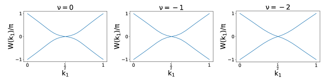
Figure S5: Wilson loop spectrum of flat bands of SK states at $\nu=0,-1,-2$.

Finally, we analyze the mean-field Hamiltonian of the symmetric Kondo state. The mean-field single-particle Hamiltonian of valley $\eta$ and spin $\uparrow$ (spin $\uparrow$ and spin $\downarrow$ are equivalent) of the Kondo symmetric state can be approximately written as

$$\tilde{H}^{(\eta)}(\mathbf{k})=\begin{bmatrix}\tilde{H}^{(f,\eta)}(\mathbf{k})&\tilde{H}^{(fc,\eta)}(\mathbf{k})\\ \tilde{H}^{(fc,\eta),{\dagger}}(\mathbf{k})&\tilde{H}^{(c,\eta)}(\mathbf{k})\end{bmatrix}$$ (S68)

$$\tilde{H}^{(f,\eta)}(\mathbf{k})=E_{f}\mathbb{I}_{2\times 2}$$

$$\tilde{H}^{(c,\eta)}(\mathbf{k})=\begin{bmatrix}E_{c}\mathbb{I}_{2\times 2}&v_{\star}(\eta k_{x}\sigma_{0}+ik_{y}\sigma_{z})\\ v_{\star}(\eta k_{x}\sigma_{0}-ik_{y}\sigma_{z})&E_{c^{\prime\prime}}\mathbb{I}_{2\times 2}\end{bmatrix}$$

$$\tilde{H}^{(fc,\eta)}(\mathbf{k})=\begin{bmatrix}\tilde{\gamma}\sigma_{0}+\tilde{v_{\star}^{\prime}}(\eta k_{x}\sigma_{x}+k_{y}\sigma_{y})&0_{2\times 2}\end{bmatrix}$$ (S69)

where $\tilde{H}^{(f,\eta)},\tilde{H}^{(c,\eta)},\tilde{H}^{(fc,\eta)}$ denote the single-particle Hamiltonian of the $f$-block, $c$-block and $fc$-block respectively. $E_{f},E_{c},E_{c^{\prime\prime}}$ denote the energy shifting induced by the Hartree term, one-body scattering term ${\hat{H}}_{cc}$ and chemical potential. $E_{f},E_{c}$ can be $\mathbf{k}$ dependent and we only keep its $\mathbf{k}$-independent part which makes dominant contributions. $E_{c^{\prime\prime}}$ comes from the Hartree contribution of ${\hat{H}}_{J}$ (Eq. S49, which is relatively small and we set $E_{c^{\prime\prime}}=0$. We also set $M=0$, since it is small compared to the other parameters. $\tilde{\gamma},\tilde{v_{\star}}^{\prime}$ denote the renormalized $f$-$c$ hybridization emerged from Kondo interactions (Eq. S37). We also drop the damping factor $e^{-|\mathbf{k}|^{2}\lambda^{2}/2}$ to simplify the analysis. In practice, we find $|\tilde{\gamma}|=\frac{1}{D_{\nu_{c},\nu_{f}}}|\gamma^{2}V_{1}^{*}+\gamma v_{\star}^{\prime}V_{2}^{*}|\approx 175\text{meV},209\text{meV},406\text{meV}$. In the chiral limit $v_{\star}^{\prime}=0$, we also have $\tilde{v_{\star}^{\prime}}=0$ ($\tilde{v_{\star}^{\prime}}=v_{\star}^{\prime}=\gamma v_{\star}^{\prime}V_{1}^{*}/D_{\nu_{c},\nu_{f}}$). We note that $|\tilde{v}_{\star}^{\prime}||\mathbf{k}|$ can reach a similar amplitude as the $k$-independent hybridization $|\tilde{\gamma}|$. However, we expect in most regions of MBZ, $|\tilde{\gamma}|$ makes the dominant contribution. We, therefore, drop the set $\tilde{v_{\star}^{\prime}}=0$ or equivalently $v_{\star}^{\prime}=0$ as an approximation. By setting $v_{\star}^{\prime}=0$, we can further separate $\tilde{H}^{(\eta)}(\mathbf{k})$ into two blocks. The first block corresponds to the row and column indices $1,3,5$ with electron operators,$f_{\mathbf{k},1\eta s},c_{\mathbf{k},1\eta s},c_{\mathbf{k},3\eta s}$. The second block corresponds to the row and column indices $2,4,6$ with electron operators,$f_{\mathbf{k},2\eta s},c_{\mathbf{k},2\eta s},c_{\mathbf{k},4\eta s}$. We focus on the first block whose single-particle Hamiltonian is

$$\tilde{h}^{(\eta)}(\mathbf{k})=\begin{bmatrix}E_{f}&\tilde{\gamma}&0\\ \tilde{\gamma}&E_{c}&v_{\star}(\eta k_{x}+ik_{y})\\ 0&v_{\star}(\eta k_{x}-ik_{y})&0\end{bmatrix}$$ (S70)

We next analyze the eigensystems of $\tilde{h}^{(\eta)}(\mathbf{k})$. We note that $\tilde{\gamma}$ provides the largest energy scales near $\Gamma_{M}$ point and will gap out $f$- and $\Gamma_{3}$ $c$-electrons. To observe this, we first consider the first $2\times 2$ block of $\tilde{h}^{(\eta)}(\mathbf{k})$ which describes the single-particle Hamiltonian of $f$- and $\Gamma_{3}$ $c$-electrons

$$\begin{bmatrix}E_{f}&\tilde{\gamma}\\ \tilde{\gamma}&E_{c}\end{bmatrix}$$ (S71)

The eigenvalues and eigenvectors are

$$E_{1} =\frac{E_{c}+E_{f}}{2}-\sqrt{\tilde{\gamma}^{2}+\frac{(E_{c}-E_{f})^{2}}{4}},\quad E_{2}=\frac{E_{c}+E_{f}}{2}+\sqrt{\tilde{\gamma}^{2}+\frac{(E_{c}-E_{f})^{2}}{4}}$$

$$v_{1} =\frac{1}{\sqrt{2E_{fc}(E_{fc}-E_{3})}}\begin{bmatrix}E_{3}-E_{fc}&\tilde{\gamma}\end{bmatrix}^{T},\quad v_{2}=\frac{1}{\sqrt{2E_{fc}(E_{fc}+E_{3})}}\begin{bmatrix}E_{3}+E_{fc}&\tilde{\gamma}\end{bmatrix}^{T}$$

where $E_{3}=\frac{E_{f}-E_{c}}{2},E_{fc}=\sqrt{\tilde{\gamma}^{2}+E_{3}^{2}}$. Since $\tilde{\gamma}$ is larger than $E_{c},E_{f}$, $\Gamma_{3}$ $c$-electrons and $f$-electrons are gapped out by the hybridization. Consequently, the flat bands are mostly formed by $\Gamma_{1}\oplus\Gamma_{2}$ $c$-electrons. Numerically, we indeed find the orbital weights of $\Gamma_{1}\oplus\Gamma_{2}$ $c$-electrons are large ($71\%,77\%,89\%$ at $\nu=0,-1,-2$ respectively).

We next treat $v_{\star}$ perturbatively. We find the dispersion of the flat band becomes

$$E_{\mathbf{k}}^{flat}\approx\frac{-E_{f}|\mathbf{k}|^{2}(v_{\star})^{2}}{E_{1}E_{2}}=\frac{E_{f}|\mathbf{k}|^{2}(v_{\star})^{2}}{\tilde{\gamma}^{2}-E_{c}E_{f}}$$ (S73)

At $\nu=0$ with particle-hole symmetry, $E_{f}=E_{c}=0$ and $E_{\mathbf{k}}^{flat}\approx 0$. However, at $\nu=-1,-2$, where $E_{f}\neq 0,E_{c}\neq 0$, flat bands become dispersive. We observe that $|E_{c}|$ is much smaller than $|\tilde{\gamma}|$ at $\nu=-1,-2$. $E_{f}$ increases as we change from $\nu=0$ to $\nu=-2$, because we are doping more holes to the $f$-orbitals. At $\nu=-2$, $E_{f}$ can reach $\sim 0.5|\tilde{\gamma}|$, but at $\nu=-1$, $E_{f}\sim 0.1|\tilde{\gamma}|$. Approximately, the dispersion of the flat band is $E_{\mathbf{k}}^{flat}\approx(v_{\star})^{2}E_{f}/\tilde{\gamma}^{2}$. At $\nu=-1$, we have $E_{\mathbf{k}}\approx 13\mathrm{meV}\cdot\mathrm{\mathring{A}^{2}}|\mathbf{k}|^{2}$ and, at $\nu=-2$, we have $E_{\mathbf{k}}\approx 45\mathrm{meV}\cdot\mathrm{\mathring{A}^{2}}|\mathbf{k}|^{2}$. This indicates a larger dispersion at $\nu=-2$, which is consistent with our numerical result shown in the main text Fig.1.

We next analyze the wavefunctions of the flat bands. The corresponding electron operator of the flat band $d^{\dagger}_{flat,\mathbf{k}}$ is

$$d^{\dagger}_{flat,\mathbf{k}}\approx\frac{1}{A_{\mathbf{k}}}\bigg{[}c^{\dagger}_{\mathbf{k},3\eta s}+\frac{v_{\star}(\eta k_{x}-ik_{y})}{E_{c}E_{f}-\tilde{\gamma}^{2}}\bigg{(}-E_{f}c^{\dagger}_{\mathbf{k},1\eta s}+\tilde{\gamma}f^{\dagger}_{\mathbf{k},1\eta s}\bigg{)}\bigg{]}$$ (S74)

where the normalization factor

$$A_{\mathbf{k}}=\sqrt{1+\frac{|v_{\star}|^{2}|\mathbf{k}|^{2}(E_{f}^{2}+\tilde{\gamma}^{2})}{(E_{c}E_{f}-\tilde{\gamma}^{2})^{2}}}$$ (S75)

We observe that in the large $|\tilde{\gamma}|$ limit, the flat bands are mostly formed by $\Gamma_{1}\oplus\Gamma_{2}$ $c$-electrons ($c_{\mathbf{k},3\eta s}^{\dagger}$). We also provide the Berry curvature derived from the wavefunction in Eq. S74

$$\Omega(\mathbf{k})=\frac{-2(E_{c}E_{f}-\tilde{\gamma}^{2})^{2}(E_{f}^{2}+\tilde{\gamma}^{2})v_{\star}^{2}}{\bigg{[}(E_{c}E_{f}-\tilde{\gamma}^{2})^{2}+(E_{f}^{2}+\tilde{\gamma}^{2})v_{\star}^{2}|\mathbf{k}|^{2}\bigg{]}^{2}}$$ (S76)

We next calculate the Wilson loop from the wavefunction in Eq. S74. The wavefunctions of $d_{flat,\mathbf{k}}^{\dagger}$ is

$$u(\mathbf{k})=\frac{1}{A_{\mathbf{k}}}\begin{bmatrix}1&\frac{v_{\star}\eta k_{x}-ik_{y}}{E_{c}E_{f}-\tilde{\gamma}^{2}}(-E_{f})&\frac{v_{\star}\eta k_{x}-ik_{y}}{E_{c}E_{f}-\tilde{\gamma}^{2}}\tilde{\gamma}\end{bmatrix}^{T}$$ (S77)

where the first, second and third rows denote $c^{\dagger}_{\mathbf{k},3\eta s},f^{\dagger}_{\mathbf{k},1\eta s},c^{\dagger}_{\mathbf{k},1\eta s}$ respectively. We then parametrize the momentum as

$$\mathbf{k}=x_{1}a_{M}\textbf{b}_{M,1}+x_{2}a_{M}\textbf{b}_{M,2},\quad\textbf{b}_{M,1}=\frac{4\pi}{3a_{M}}(\sqrt{3},0),\quad\textbf{b}_{M,2}=\frac{4\pi}{3a_{M}}(\frac{\sqrt{3}}{2},\frac{3}{2})$$ (S78)

$$x_{1},x_{2}\in[-\frac{1}{2},\frac{1}{2}]\frac{1}{a_{M}}$$ (S79)

and define $|u(x_{1},x_{2})\rangle$ as $|u(\mathbf{k})\rangle$ with $\mathbf{k}=x_{1}a_{M}\textbf{b}_{M,1}+x_{2}a_{M}\textbf{b}_{M,2}$. The Wilson loop can be written as

$$W(x_{1})=\prod_{j=0}^{N-1}\langle u(x_{1},x_{2}=x_{2,i})|u(x_{1},x_{2}=x_{2,j+1}\rangle\langle u(x_{1},x_{2,N})|u(x_{1},x_{2,0})\rangle,\quad x_{2,i}=-\frac{1}{2a_{M}}+\frac{1}{a_{M}}\frac{i}{N}$$ (S80)

The spectrum of the Wilson loop is

$$N(x_{1})=-i\ln(W(x_{1}))=-i\int_{-\frac{1}{2a_{M}}}^{\frac{1}{2a_{M}}}\langle u(x_{1},x_{2})|\partial_{x_{2}}|u(x_{1},x_{2})\rangle dx_{2}-i\ln(\langle u(x_{1},1/(2a_{M}))|u(x_{1},-1/(2a_{M})\rangle)$$ (S81)

In the continuous limit with $a_{M}\rightarrow 0$, we find

$$N(x_{1})=-i\int_{-\infty}^{\infty}\langle u(x_{1},x_{2})|\partial_{x_{2}}|u(x_{1},x_{2})\rangle dx_{2}-i\ln(\langle u(x_{1},\infty)|u(x_{1},-\infty\rangle)$$ (S82)

Combining Eq. S77 and Eq. S82, we find

$$N(x_{1})= \pi\bigg{(}1+\frac{v_{\star}^{2}x_{1}}{\sqrt{x_{1}^{2}v_{\star}^{2}+\frac{(\tilde{\gamma}^{2}-E_{c}E_{f})^{2}}{E_{f}^{2}+\tilde{\gamma}^{2}}}}\bigg{)}$$ (S83)

Even though Eq. S82 is calculated from the perturbative wavefunction in Eq. S77, it qualitatively captures the behaviors of the Wilson loop shown in Fig. S5. We observe that $N(-\infty)=0$ and $N(\infty)=2\pi$, which indicates a $2\pi$ winding at $\nu=0,-1,-2$. We also mention that current calculations correspond to one of the two flat bands for each valley and each spin, because we only pick one block of the single-particle Hamiltonian as we discussed near Eq. S70. The other flat band can be derived in the same manner and has similar behaviors, since it has a similar single-particle Hamiltonian.

S5 Mean-field solutions of the topological heavy-fermion model

We now discuss the mean-field equations of topological heavy-fermion mode in Eq. S12. We use a similar Hartree-Fock approximation as introduced in Ref. Song and Bernevig (2022). However, we decouple ${\hat{H}}_{J}$ via Eq. S50. The mean-field expectation values we considered are

$$O^{f}_{\alpha\eta s,\alpha^{\prime}\eta^{\prime}s^{\prime}}=\frac{1}{N_{M}}\sum_{\mathbf{R}}\langle\Psi|:f_{\mathbf{R},\alpha\eta s}^{\dagger}f_{\mathbf{R},\alpha^{\prime}\eta^{\prime}s^{\prime}}:|\Psi\rangle$$

$$O^{c^{\prime}}_{a\eta s,a^{\prime}\eta^{\prime}s^{\prime}}=\frac{1}{N_{M}}\sum_{|\mathbf{k}|<\Lambda_{c}}\langle\Psi|:c_{\mathbf{k},a\eta s}^{\dagger}c_{\mathbf{k},a^{\prime}\eta^{\prime}s^{\prime}}:|\Psi\rangle,\quad a\in\{1,2\}$$

$$O^{c^{\prime\prime}}_{a\eta s,a^{\prime}\eta^{\prime}s^{\prime}}=\frac{1}{N_{M}}\sum_{|\mathbf{k}|<\Lambda_{c}}\langle\Psi|:c_{\mathbf{k},a+2\eta s}^{\dagger}c_{\mathbf{k},a^{\prime}+2\eta^{\prime}s^{\prime}}:|\Psi\rangle,\quad a,a^{\prime}\in\{1,2\}$$

$$O^{c^{\prime}f}_{a\eta s,\alpha^{\prime}\eta^{\prime}s^{\prime}}=\frac{1}{\sqrt{N}N}\sum_{|\mathbf{k}|<\Lambda_{c},\mathbf{R}}e^{-i\mathbf{k}\cdot\mathbf{R}}\langle\Psi|c_{\mathbf{k},a\eta s}^{\dagger}f_{\mathbf{R},\alpha^{\prime}\eta^{\prime}s^{\prime}}|\Psi\rangle,\quad a\in\{1,2\}$$

$$V_{3}=\sum_{\mathbf{R},|\mathbf{k}|<\Lambda_{c}}\sum_{\alpha\eta,s}\frac{e^{i\mathbf{k}\cdot\mathbf{R}}\delta_{1,\eta(-1)^{\alpha+1}}}{{N_{M}}\sqrt{N_{M}}}\langle\Psi|f_{\mathbf{R},\alpha\eta s}^{\dagger}c_{\mathbf{k},\alpha+2\eta s}|\Psi\rangle$$

$$V_{4}=\sum_{\mathbf{R},|\mathbf{k}|<\Lambda_{c}}\sum_{\alpha\eta,s}\frac{e^{i\mathbf{k}\cdot\mathbf{R}}\delta_{-1,\eta(-1)^{\alpha+1}}}{{N_{M}}\sqrt{N_{M}}}\langle\Psi|\eta f_{\mathbf{R},\alpha\eta s}^{\dagger}c_{\mathbf{k},\alpha+2\eta s}|\Psi\rangle$$ (S84)

where $O^{f},O^{c^{\prime\prime}},V_{3},V_{4}$ have also been used in the Kondo lattice mean-field calculations (Eq. S38, Eq. S48 and Eq. S44).

In addition, THF model also has a chemical potential term ${\hat{H}}_{\mu}$ (Eq. S21) and we determine $\mu$ by requiring the total filling of $f$- and $c$-electrons to be $\nu$:

$$\nu=\text{Tr}[O^{f}]+\text{Tr}[O^{c^{\prime}}]+\text{Tr}[O^{c^{\prime\prime}}]$$ (S85)

where we note that the filling of $f$-, $\Gamma_{3}$ $c$- and $\Gamma_{1}\oplus\Gamma_{2}$ $c$-electrons are

$$\nu_{f}=\text{Tr}[O^{f}],\quad\nu_{c^{\prime}}=\text{Tr}[O^{c^{\prime}}],\quad\nu_{c^{\prime\prime}}=\text{Tr}[O^{c^{\prime\prime}}]\,,$$ (S86)

respectively.

We discuss the difference and similarities between the mean-field equations of the KL model and that of the THF model. For the THF model, we introduce mean fields $O^{f},O^{c^{\prime}},O^{c^{\prime\prime}},O^{c^{\prime}f},V_{3},V_{4}$ (Eq. S84) (for a generic state without enforcing any symmetries). As for KL model, we introduce mean fields $V_{1},V_{2},O^{f},O^{c^{\prime},1},O^{c^{\prime},2},O^{c^{\prime\prime}},V_{3},V_{4}$ (Eq. S38, Eq. S35, Eq. S48, Eq. S44) (for a generic state without enforcing any symmetry).

• For both models, $O^{c^{\prime\prime}},O^{f},V_{3},V_{4}$ are part of mean fields and contribute the mean-field decoupling of ${\hat{H}}_{J}$ (Eq. S50).

• In the THF model, we introduce a chemical potential term $\mu$ that couples to both the $f$-electron density operators and $c$-electron density operator (Eq. S21. We enforce the total filling of $f$- and $c$-electrons to be $\nu$ by tuning $\mu$. In the KL model, we introduce a Lagrangian multiplier $\lambda_{f}$ (Eq. S51) that couples to $f$-electron density operators, and a chemical potential $\mu_{c}$ (Eq. S28) that couples to the $c$-electron density operators. We enforce the fillings of $f$-electrons and $c$-electrons to be $\nu_{f}$ and $\nu_{c}$ respectively by tuning $\lambda_{f}$ and $\mu_{c}$ in the KL model.

• We also mention that $O^{c^{\prime}}$ in THF model (Eq. S84) and $O^{c^{\prime},1}$ in the KL model (Eq. S38) are different, where the latter one has included an additional damping factor $e^{-|\mathbf{k}|^{2}\lambda^{2}}$.

• In the THF model, we do not need hybridization fields $V_{1},V_{2}$ (Eq. S35), since both come from the decoupling of Kondo interactions that only appear in the KL model.

S5.1 Mean-field equations of fully symmetric state

We next discuss the solution of the symmetric state The fully symmetric state is characterized by density matrices $O^{f},O^{c^{\prime}},O^{c^{\prime\prime}},O^{c^{\prime}f}$ and hybridization fields $V_{3},V_{4}$ that satisfy all symmetries. The structures of $O^{f},O^{c^{\prime\prime}}$ in the fully symmetric state are given in Eq. S60. We also prove that $V_{3}=V_{4}=0$ in a fully symmetric state (near Eq. S62). We now discuss the symmetry properties of $O^{c^{\prime}},O^{c^{\prime}f}$. From Eq. S32, a $U(1)_{v}$ symmetric solution satisfies

$$O^{c^{\prime}}_{a\eta s,\alpha^{\prime}\eta^{\prime}s^{\prime}}=O^{c^{\prime}}_{a\eta s,\alpha^{\prime}\eta^{\prime}s^{\prime}}e^{-i\theta_{\nu}(\eta-\eta^{\prime})}\Rightarrow O^{c^{\prime}}_{a\eta s,\alpha-\eta s^{\prime}}=0$$

$$O^{c^{\prime}f}_{a\eta s,\alpha^{\prime}\eta^{\prime}s^{\prime}}=O^{c^{\prime}f}_{a\eta s,\alpha^{\prime}\eta^{\prime}s^{\prime}}e^{-i\theta_{\nu}(\eta-\eta^{\prime})}\Rightarrow O^{c^{\prime}f}_{a\eta s,\alpha-\eta s^{\prime}}=0$$ (S87)

Then, $O^{c^{\prime}},O^{c^{\prime}f}$ is block diagonalized in valley indices. We next consider a $SU(2)_{\eta}$ transformation acting on the valley $\eta$. It indicates

$$\sum_{s,s^{\prime}}[e^{i\sum_{\mu}\theta^{\eta}_{\mu}\sigma^{\mu}}]_{s_{2},s}O^{c^{\prime}}_{\alpha\eta s,\alpha^{\prime}\eta s^{\prime}}[e^{i\sum_{\mu}\theta^{\eta}_{\mu}\sigma^{\mu}}]_{s^{\prime},s_{2}^{\prime}}=O^{c^{\prime}}_{\alpha\eta s_{2},\alpha^{\prime}\eta s_{2}^{\prime}}\Rightarrow O^{c^{\prime}}_{\alpha\eta s,\alpha^{\prime}\eta s^{\prime}}$$

$$\sum_{s,s^{\prime}}[e^{i\sum_{\mu}\theta^{\eta}_{\mu}\sigma^{\mu}}]_{s_{2},s}O^{c^{\prime}f}_{\alpha\eta s,\alpha^{\prime}\eta s^{\prime}}[e^{i\sum_{\mu}\theta^{\eta}_{\mu}\sigma^{\mu}}]_{s^{\prime},s_{2}^{\prime}}=O^{c^{\prime}f}_{\alpha\eta s_{2},\alpha^{\prime}\eta s_{2}^{\prime}}\Rightarrow O^{c^{\prime}f}_{\alpha\eta s,\alpha^{\prime}\eta s^{\prime}}$$ (S88)

Combining Eq. S87 and Eq. S88, we can introduce $2\times 2$ matrices $o^{c^{\prime},\eta},o^{c^{\prime}f,\eta}$, such that

$$O^{c^{\prime}}_{\alpha\eta s,\alpha^{\prime}\eta^{\prime}s^{\prime}}=o^{c^{\prime}}_{\alpha,\alpha^{\prime}}\delta_{s,s^{\prime}}\delta_{\eta,\eta^{\prime}},\quad O^{c^{\prime}f}_{\alpha\eta s,\alpha^{\prime}\eta^{\prime}s^{\prime}}=o^{c^{\prime}f}_{\alpha,\alpha^{\prime}}\delta_{s,s^{\prime}}\delta_{\eta,\eta^{\prime}}$$ (S89)

We now consider the effect of discrete symmetries in Eq. S30. Using Eq. S31 and Eq. S89, we find

$$T: \quad(o^{c^{\prime},\eta})^{*}=o^{c^{\prime},-\eta},\quad(o^{c^{\prime}f,\eta})^{*}=o^{c^{\prime}f,-\eta}$$

$$C_{3z}: \quad e^{i2\pi/3\eta\sigma_{z}}o^{c^{\prime},\eta}e^{-i2\pi\eta/3\sigma_{z}}=o^{c^{\prime},\eta},\quad e^{i2\pi/3\eta\sigma_{z}}o^{c^{\prime}f,\eta}e^{-i2\pi\eta/3\sigma_{z}}=o^{c^{\prime}f,\eta}$$

$$C_{2x}: \quad\sigma_{x}o^{c^{\prime},\eta}\sigma_{x}=o^{c^{\prime},\eta},\quad\sigma_{x}o^{c^{\prime}f,\eta}\sigma_{x}=o^{c^{\prime}f,\eta}$$

$$C_{2z}T: \quad\sigma_{x}(o^{c^{\prime},\eta})^{*}\sigma_{x}=o^{c^{\prime},\eta},\quad\sigma_{x}(o^{c^{\prime}f,\eta})^{*}\sigma_{x}=o^{c^{\prime}f,\eta}$$ (S90)

Then we can introduce a single real number $\chi_{0}^{c^{\prime}},\chi_{0}^{c^{\prime}f}$ to characterize the density matrices

$$O^{c^{\prime}}_{\alpha\eta s,\alpha^{\prime}\eta^{\prime}s^{\prime}}=\chi_{0}^{c^{\prime}}\delta_{\alpha,\alpha^{\prime}}\delta_{\eta,\eta^{\prime}},\quad O^{c^{\prime}f}_{\alpha\eta s,\alpha^{\prime}\eta^{\prime}s^{\prime}}=\chi_{0}^{c^{\prime}f}\delta_{\alpha,\alpha^{\prime}}\delta_{\eta,\eta^{\prime}}\delta_{s,s^{\prime}}\,.$$ (S91)

Since the filling of $\Gamma_{3}$ $c$-electrons is $\nu_{c^{\prime}}=\text{Tr}[O^{c^{\prime}}]=8\chi_{0}^{c^{\prime}}$, we let $\chi_{0}^{c^{\prime}}=\nu_{c^{\prime}}/8$. Therefore, instead of calculating the original density matrices in Eq. S84, we can calculate the following quantities

$$\nu_{f}=\frac{1}{N_{M}}\sum_{\mathbf{R},\alpha\eta s}\langle\Psi|:f_{\mathbf{R},\alpha\eta s}^{\dagger}f_{\mathbf{R},\alpha\eta s}:|\Psi\rangle$$

$$\nu_{c^{\prime}}=\frac{1}{N_{M}}\sum_{|\mathbf{k}|<\Lambda_{c},a=1,2,\eta s}\langle\Psi|:c_{\mathbf{k},a\eta s}^{\dagger}c_{\mathbf{k},a\eta s}:|\Psi\rangle$$

$$\nu_{c^{\prime\prime}}=\frac{1}{N_{M}}\sum_{|\mathbf{k}|<\Lambda_{c},a=3,4,\eta s}\langle\Psi|:c_{\mathbf{k},a\eta s}^{\dagger}c_{\mathbf{k},a\eta s}:|\Psi\rangle$$

$$\chi^{c^{\prime}f}=\frac{1}{8N_{M}\sqrt{N_{M}}}\sum_{|\mathbf{k}|<\Lambda_{c},\mathbf{R},\alpha\eta s}e^{-i\mathbf{k}\cdot\mathbf{R}}\langle\Psi|c^{\dagger}_{\mathbf{k},\alpha\eta s}f_{\mathbf{R},\alpha\eta s}|\Psi\rangle$$ (S92)

and construct density matrices via Eq. S60 and Eq. S91. In addition, the filling constraints in Eq. S85 becomes

$$\nu=\nu_{f}+\nu_{c^{\prime}}+\nu_{c^{\prime\prime}}$$ (S93)

Combining Eq. S92 and Eq. S93, we have a complete set of the mean-field self-consistent equations of symmetric state.

Here we discuss the differences and similarities between the symmetric solution in the KL model (Sec. S4.5) and the symmetric solution in the THF model as introduced in this section.

• Both Kondo symmetric (KS) state in KL model and the symmetric state in the THF model preserve all the symmetries.

• The KS state is adiabatically connected to the symmetric state in the THF model.

• The mean-field solutions are exact at $N=\infty$.

• To obtain a more precise description of the Kondo state, we need to introduce a Gutzwiller projector to our symmetric-state wavefunction in the THF model. The Gutzwiller projector will suppress the charge fluctuations of $f$-electrons and is expected to further lower the energy of the symmetric state.

• We also comment that, in the THF model, the flat bands are mainly formed by $f$-electrons with $f$-electron orbital weights $80\%$, $85\%$ and $87\%$ at $\nu=0,-1,-2$ respectively. However, in the KL model, the flat bands are mainly formed by $\Gamma_{1}\oplus\Gamma_{2}$ electrons as discussed in Sec. S4.5. This is because, in the KL model, we observed an enhanced $f$-$c$ hybridization driven by Kondo interactions which is absent in the symmetric state solution of THF model. We expect the enhanced hybridization will be recovered after introducing the Gutzwiller projector.

• We find the spectrum of the Wilson loop in the symmetric state of the THF model has winding number one and three crossing points(Fig. S6). However, in the SK state of the KL model, the spectrum of the Wilson loop spectrum has winding number one and one crossing point (Fig. S5). However, at $\nu=0$, for both the THF model and the KL model, the symmetric state has a stable topology with an odd Winding number of Wilson loop spectrum Song et al. (2019). We also mention the difference in the Wilson loop spectrum comes from the absence of enhanced $f$-$c$ hybridization in the THF model.

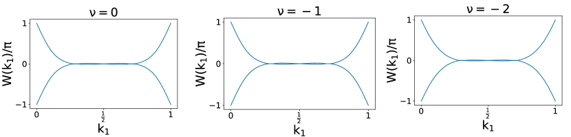
Figure S6: Wilson loop spectrum of symmetric state in the THF model at $\nu=0,-1,-2$

S5.2 Mean-field equations of the symmetric state in the presence of strain

We now discuss the mean-field solution of the symmetric state in the presence of strain. We add the following term to the Hamiltonian (Eq. S12)

$${\hat{H}}_{strain}=\alpha\sum_{\mathbf{R},\eta s}(f_{\mathbf{R},1\eta s}^{\dagger}f_{\mathbf{R},2\eta s}+\text{h.c.})$$ (S94)

We note that ${\hat{H}}_{strain}$ only breaks $C_{3z}$ symmetry. To show this, we rewrite the ${\hat{H}}_{strain}$ as

$${\hat{H}}_{strain}=\sum_{\mathbf{R},\alpha\eta s,\alpha^{\prime}\eta^{\prime}s^{\prime}}\alpha f_{\mathbf{R},\alpha\eta s}^{\dagger}[h_{strain}]_{\alpha\eta s,\alpha^{\prime}\eta^{\prime}s^{\prime}}f_{\mathbf{R},\alpha^{\prime}\eta^{\prime}s^{\prime}}$$

$$h_{strain}=\sigma_{x}\tau_{0}\varsigma_{0}$$ (S95)

where the matrix structure of ${\hat{H}}_{strain}$ is denoted by $h_{strain}\sigma_{x}\tau_{0}\varsigma_{0}$. We now show it commutes with $D^{f}(T),D^{f}(C_{2x}),D^{f}(C_{2z}T),D^{f}(g_{SU(2)_{\eta}}(\theta_{\eta}^{\mu})),D^{f}(g_{U(1)_{v}}((\theta_{v})),D^{f}(g_{U(1)_{c}}((\theta_{c}))$ (Eq. S31, Eq. S32) and hence ${\hat{H}}_{strain}$ preserves all symmetries except for $C_{3z}$

$$[h_{strain},D^{f}(T)]=[\sigma_{x}\tau_{0}\varsigma_{0},\sigma_{0}\tau_{x}\varepsilon_{0}]=0$$

$$[h_{strain},D^{f}(C_{2x})]=[\sigma_{x}\tau_{0}\varsigma_{0},\sigma_{x}\tau_{0}\varsigma_{0}]=0$$

$$[h_{strain},D^{f}(C_{2z}T)]=[\sigma_{x}\tau_{0}\varsigma_{0},\sigma_{x}\tau_{0}\varsigma_{0}]=0$$

$$[h_{strain},D^{f}(g_{U(1)_{c}}((\theta_{c}))]=[\sigma_{x}\tau_{0}\varsigma_{0},e^{-i\theta_{c}}\sigma_{0}\tau_{0}\varsigma_{0}]=0$$

$$[h_{strain},D^{f}(g_{U(1)_{v}}((\theta_{v}))]=[\sigma_{x}\tau_{0}\varsigma_{0},\sigma_{0}e^{-i\theta_{v}\tau_{z}}\varsigma_{0}]=0$$

$$[h_{strain},D^{f}(g_{SU(2)_{\eta}}(\theta_{\eta}^{\mu}))]=[\sigma_{x}\tau_{0}\varsigma_{0},\sigma_{0}e^{-i\sum_{\mu}\theta_{\mu}^{\eta}\frac{\tau_{0}+\eta\tau_{z}}{4}\varsigma_{\mu}}]=0$$

In the presence of strain, the symmetric state is defined as the state that preserves all the symmetries except for $C_{3z}$ which is broken by the strain. In the presence of $C_{3z}$-breaking strain, Eq. S57 and Eq. S89 still hold, because the system still has $U(1)_{c}\times U(1)_{v}\times SU(2)_{+}\times SU(2)_{-}$ symmetry. As for Eq. S58 and Eq. S90, we only need to consider $T,C_{2x},C_{2z}T$ and we find

$$O^{f}_{\alpha\eta s,\alpha^{\prime}\eta^{\prime}s^{\prime}}=\bigg{[}\chi_{0}^{f}\sigma_{0}+\chi_{1}^{f}\sigma_{x}\bigg{]}_{\alpha,\alpha^{\prime}}\delta_{\eta,\eta^{\prime}}\delta_{s,s^{\prime}}$$

$$O^{c^{\prime}}_{\alpha\eta s,\alpha^{\prime}\eta^{\prime}s^{\prime}}=\bigg{[}\chi_{0}^{c^{\prime}}\sigma_{0}+\chi_{1}^{c^{\prime}}\sigma_{x}\bigg{]}_{\alpha,\alpha^{\prime}}\delta_{\eta,\eta^{\prime}}\delta_{s,s^{\prime}},\quad O^{c^{\prime\prime}}_{\alpha\eta s,\alpha^{\prime}\eta^{\prime}s^{\prime}}=\bigg{[}\chi_{0}^{c^{\prime\prime}}\sigma_{0}+\chi_{1}^{c^{\prime\prime}}\sigma_{x}\bigg{]}_{\alpha,\alpha^{\prime}}\delta_{\eta,\eta^{\prime}}\delta_{s,s^{\prime}},$$

$$O^{c^{\prime}f}_{\alpha\eta s,\alpha^{\prime}\eta^{\prime}s^{\prime}}=\bigg{[}\chi_{0}^{c^{\prime}f}\sigma_{0}+\chi_{1}^{c^{\prime}f}\sigma_{x}\bigg{]}_{\alpha,\alpha^{\prime}}\delta_{\eta,\eta^{\prime}}\delta_{s,s^{\prime}}$$ (S96)

where $\chi_{0}^{f},\chi_{1}^{f},\chi_{0}^{c^{\prime}},\chi_{1}^{c^{\prime}},\chi_{0}^{c^{\prime\prime}},\chi_{1}^{c^{\prime\prime}},\chi_{0}^{c^{\prime}f},\chi_{1}^{c^{\prime}f}$ are real numbers tha characterize the density matrices. Combining Eq. S38, Eq. S48 and Eq. S96, we find

$$\chi_{0}^{f}=\frac{1}{8N_{M}}\sum_{\mathbf{R},\alpha etas}\langle\Psi|:f_{\mathbf{R},\alpha\eta s}^{\dagger}f_{\mathbf{R},\alpha\eta s}:|\Psi\rangle,\quad\chi_{1}^{f}=\frac{1}{8N_{M}}\sum_{\mathbf{R},\eta s}\langle\Psi|f_{\mathbf{R},1\eta s}^{\dagger}f_{\mathbf{R},2\eta s}+f_{\mathbf{R},2\eta s}^{\dagger}f_{\mathbf{R},1\eta s}|\Psi\rangle$$

$$\chi_{0}^{c^{\prime}}=\frac{1}{8N_{M}}\sum_{|\mathbf{k}|<\Lambda_{c},=1,2,\eta s}\langle\Psi|:c_{\mathbf{k},a\eta s}^{\dagger}c_{\mathbf{k},a\eta s}^{\dagger}:|\Psi\rangle,\quad\chi_{1}^{c^{\prime}}=\frac{1}{8N_{M}}\sum_{|\mathbf{k}|<\Lambda_{c},\eta s}\langle\Psi|c_{\mathbf{k},1\eta s}^{\dagger}c_{\mathbf{k},2\eta s}+c_{\mathbf{k},2\eta s}^{\dagger}c_{\mathbf{k},1\eta s}|\Psi\rangle$$

$$\chi_{0}^{c^{\prime\prime}}=\frac{1}{8N_{M}}\sum_{|\mathbf{k}|<\Lambda_{c},=3,4,\eta s}\langle\Psi|:c_{\mathbf{k},a\eta s}^{\dagger}c_{\mathbf{k},a\eta s}^{\dagger}:|\Psi\rangle,\quad\chi_{1}^{c^{\prime\prime}}=\frac{1}{8N_{M}}\sum_{|\mathbf{k}|<\Lambda_{c},\eta s}\langle\Psi|c_{\mathbf{k},3\eta s}^{\dagger}c_{\mathbf{k},4\eta s}+c_{\mathbf{k},4\eta s}^{\dagger}c_{\mathbf{k},3\eta s}|\Psi\rangle$$

$$\chi_{0}^{c^{\prime}f}=\frac{1}{8N_{M}\sqrt{N_{M}}}\sum_{|\mathbf{k}|<\Lambda_{c},\mathbf{R},\alpha\eta s}e^{-i\mathbf{k}\cdot\mathbf{R}}\langle\Psi|c^{\dagger}_{\mathbf{k},\alpha\eta s}f_{\mathbf{R},\alpha\eta s}|\Psi\rangle,\quad$$

$$\chi_{1}^{c^{\prime}f}=\frac{1}{8N_{M}\sqrt{N_{M}}}\sum_{|\mathbf{k}|<\Lambda_{c},\mathbf{R},\eta s}e^{-i\mathbf{k}\cdot\mathbf{R}}\langle\Psi|c^{\dagger}_{\mathbf{k},1\eta s}f_{\mathbf{R},2\eta s}+c^{\dagger}_{\mathbf{k},2\eta s}f_{\mathbf{R},1\eta s}|\Psi\rangle$$

$$\chi_{0}^{c^{\prime\prime}f}=\frac{1}{8N_{M}\sqrt{N_{M}}}\sum_{|\mathbf{k}|<\Lambda_{c},\mathbf{R},\alpha\eta s}e^{-i\mathbf{k}\cdot\mathbf{R}}\langle\Psi|c^{\dagger}_{\mathbf{k},\alpha+2\eta s}f_{\mathbf{R},\alpha\eta s}|\Psi\rangle,\quad$$

$$\chi_{1}^{c^{\prime\prime}f}=\frac{1}{8N_{M}\sqrt{N_{M}}}\sum_{|\mathbf{k}|<\Lambda_{c},\mathbf{R},\eta s}e^{-i\mathbf{k}\cdot\mathbf{R}}\langle\Psi|c^{\dagger}_{\mathbf{k},3\eta s}f_{\mathbf{R},2\eta s}+c^{\dagger}_{\mathbf{k},4\eta s}f_{\mathbf{R},3\eta s}|\Psi\rangle$$ (S97)

where we also have $\chi_{0}^{f}=\nu_{f}/8,\chi_{0}^{c^{\prime}}=\nu_{c^{\prime}}/8,\chi_{0}^{c^{\prime\prime}}=\nu_{c^{\prime\prime}}/8$. As for $V_{3},V_{4}$, we only consider the $T,C_{2x},C_{z}T$ of Eq. S61, which indicates

$$V_{3}=V_{4}=V_{3}^{*}=V_{4}^{*}$$ (S98)

Combining Eq. S44, Eq. S93, Eq. S97 and Eq. S98 with filling constraints $\nu=\nu_{f}+\nu_{c^{\prime}}+\nu_{c^{\prime\prime}}$, we have a complete set of the mean-field self-consistent equations of symmetric state in the presence of strain. We perform calculations with non-zero strain at $\nu=0,-1,-2,-3$. We initialize the calculations with the fully symmetric solutions derived at zero strain, and the procedure converges within 500 iterations. The results are illustrated and discussed in Sec. S5.4.

S5.3 Effect of doping

We now discuss the effect of doping at zero strain. For hole doping at $\nu=0,-1,-2,-3$ and electron doping at $\nu=0$, we mainly dope electrons to the light bands that are mostly formed by $c$-electrons (Fig. S7). Consequently, the energy difference between the symmetric state and the ordered state decreases since we have more conduction $c$-electrons near the Fermi energy, and the system favors the symmetric state.

We now point out the complexity of electron dopings at $\nu=-1,-2$. Doping electrons at $\nu=-1,-2$ is equivalent to dope electrons to the heavy bands that are mostly formed by $f$-electrons (Fig. S7). The heavy (flat) bands become closer to the Fermi energy, and hence, the energy cost of putting $f$-electrons into flat bands will be small. Then we can fill the heavy (flat) bands with a small energy cost. By filling the heavy (flat) bands, the type of orders formed by $f$-electrons can change a lot. To observe the change of the ordered states, we consider the following order parameters

$$O_{x}=\frac{1}{N_{M}}\sum_{\mathbf{R},\alpha\eta s,\alpha^{\prime}\eta^{\prime}s^{\prime}}f_{\mathbf{R},\alpha\eta s}^{\dagger}[o_{x}]_{\alpha\eta s,\alpha^{\prime}\eta^{\prime}s^{\prime}}f_{\mathbf{R},\alpha^{\prime}\eta^{\prime}s^{\prime}},\quad x\in\{KIVC,S_{z},V_{z},V_{y}\}$$

$$o_{KIVC}=\sigma_{y}\tau_{y}\varsigma_{0},\quad o_{S_{z}}=\sigma_{0}\tau_{0}\varsigma_{z},\quad o_{V_{z}}=\sigma_{0}\tau_{z}\varsigma_{0},\quad o_{V_{y}}=\sigma_{0}\tau_{y}\varsigma_{0}$$ (S99)

We measure the expectation values of $O_{x=KIVC,S_{z},V_{z},V_{y}}$ with respect to the ordered states at each filling. In Fig. S8, we show the evolution of $\langle O_{x}\rangle$ as a function of doping. We find for hole doping at $\nu=0,-1,-2$ and electron doping at $\nu=0$ (where carriers go to light bands in both cases), the system stays in the same ordered states (compared to the integer filling). However, for electron doping at $\nu=-1,-2$, we can observe the changes of the order parameters. This is because we are mainly dope $f$-electrons for electron doping at $\nu=-1,-2$. We thus conclude that electron doping at $\nu=-1,-2$ will introduce sizeable changes of the order parameters. Both the change of order parameters and the doping effect will affect the energy competition between the symmetric state and the ordered state.

Finally, we comment on the $\nu=-3$ case. At $\nu=-3$, the actual ground state might be a CDW state which breaks the translational symmetry Xie et al. (2022) and is beyond our current consideration. In addition, at $\nu=-3$, even for the valley polarized state we currently considered, electron doping is equivalent to doping both heavy and light bands (Fig. S7), which is different from $\nu=-1,-2$. We leave the detailed study of $\nu=-3$ for future study.

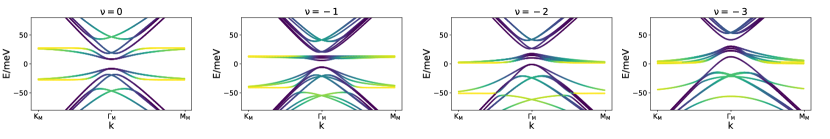
Figure S7: Dipsersions of KIVC state at $\nu=0$, KIVC+VP state at $\nu=-1$, KIVC state at $\nu=-2$ and VP state at $\nu=-3$. The color represents the weight of $f$-(yellow) and $c$-(blue) electrons.

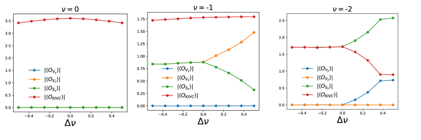
Figure S8: Evolution of order parameter as a function of doping at $\nu=0,-1,-2$

S5.4 Effect of strain

We next analyze the effect of the strain. We first note that as we increase $\alpha$ (Eq. S95), the strain will gradually suppress the KIVC order ($O^{KIVC}$, Eq. S99). This can be observed from

$$\{o_{KIVC},h_{strain}\}=\{\sigma_{y}\tau_{y}\varsigma_{0},\sigma_{x}\tau_{0}\varsigma_{0}\}=0$$ (S100)

Heuristically, the anti-commuting nature indicates the competition between $o_{KIVC}$ and $h_{strain}$. Thus, as we increase $h_{strain}$, $o_{KIVC}$ will be suppressed. We also find the spin-polarization $O_{S_{z}}$ and valley polarization $O_{V_{z}}$ commute with $h_{strain}$

$$[o_{S_{z}},h_{strain}]=[\sigma_{0}\tau_{0}\varsigma_{z},\sigma_{x}\tau_{0}\varsigma_{0}]=0,\quad[o_{V_{z}},h_{strain}]=[\sigma_{0}\tau_{z}\varsigma_{0},\sigma_{x}\tau_{0}\varsigma_{0}]=0$$ (S101)

Heuristically, this indicates the valley and spin polarization do not directly compete with $h_{strain}$. However, as we will show in this section, a sufficiently large strain could still destroy the valley and spin polarization in the THF model.

For future convenience, we also introduce the eigenstates of the strain Hamiltonian ${\hat{H}}_{strain}$ (Eq. S95)

$$d_{\mathbf{R},1\eta s}^{\dagger}=\frac{1}{\sqrt{2}}(f_{\mathbf{R},1\eta s}^{\dagger}-f_{\mathbf{R},2\eta s}^{\dagger}),\quad d_{\mathbf{R},2\eta s}^{\dagger}=\frac{1}{\sqrt{2}}(f_{\mathbf{R},1\eta s}^{\dagger}+f_{\mathbf{R},2\eta s}^{\dagger})$$ (S102)

We will call $d_{\mathbf{R},1\eta s}^{\dagger}$ and $d_{\mathbf{R},2\eta s}^{\dagger}$ as $d_{1}$ and $d_{2}$ electrons (orbitals), respectively, for short. We mention that $d_{1},d_{2}$ are $f$-electrons. The strain Hamiltonian can then be written as

$${\hat{H}}_{strain}=\alpha\sum_{\mathbf{R},\alpha\eta s}(-d_{\mathbf{R},1\eta s}^{\dagger}d_{\mathbf{R},1\eta s}+d_{\mathbf{R},2\eta s}^{\dagger}d_{\mathbf{R},2\eta s})$$ (S103)

Thus, for a positive strain amplitude $\alpha>0$, the energy of $d_{1}$ electrons will be lowered and the energy of $d_{2}$ electrons will be raised. We introduce $\langle h_{strain}\rangle$ to characterize the population imbalance between $d_{1}$ and $d_{2}$ electrons

$$\langle h_{strain}\rangle=\langle\frac{1}{N_{M}}\sum_{\mathbf{R},\alpha\eta s,\alpha^{\prime}\eta^{\prime}s^{\prime}}f_{\mathbf{R},\alpha\eta s}^{\dagger}[h_{strain}]_{\alpha\eta s,\alpha^{\prime}\eta^{\prime}s^{\prime}}f_{\mathbf{R},\alpha^{\prime}\eta^{\prime}s^{\prime}}\rangle=\frac{1}{N_{M}}\sum_{\mathbf{R},\alpha\eta s}\langle d_{\mathbf{R},1\eta s}^{\dagger}d_{\mathbf{R},1\eta s}-d_{\mathbf{R},2\eta s}^{\dagger}d_{\mathbf{R},2\eta s}\rangle\,$$ (S104)

In Fig. S9, we plot the evolution of various order parameters and also $|\langle h_{strain}\rangle|$ where the expectation value is taken with respect to the ordered state solution. In all cases, $|\langle h_{strain}\rangle|$ increases as we increase $\alpha$, since $\alpha$ linearly coupled to $h_{strain}$ term. The KIVC order will be suppressed and fully destroyed at sufficient strong strain at $\nu=0,-1,-2$. At $\nu=0$, after the destruction of the KIVC order, self-consistent calculation produces a symmetric ground state that only breaks $C_{3z}$ symmetry, even though we initialize the mean-field calculation with an ordered state.

However, at $\nu=-1,-2$, after the destruction of KIVC order, the spin polarization and valley polarization still exist. By further increasing the strain, the ordered states will finally become unstable (Fig. S9), which means the mean-field calculations that are initialized with ordered solutions converge to a symmetric state.

We next analyze the transition from an ordered state to a symmetric state at a large strain at $\nu=-1,-2$.

S5.4.1 $\nu=-1$

We first consider the $\nu=-1$ with $4\text{meV}\lesssim\alpha\lesssim 18\text{meV}$. In this parameter region, the KIVC order is destroyed but valley and spin polarization persist (Fig. S9). In Fig. S10 (a) (b), we plot the band structures in this parameter region. We note that flat bands that are mostly formed by $f$-electrons (marked by red circles, Fig. S10) move towards the Fermi level, as we increase strain. Near the transition point to the symmetric state, the flat bands are very close to the Fermi level. This signals an instability of the ordered states since we can fill the flat band without any energy cost. By diagonalizing the mean-field Hamiltonian, we find the flat bands (marked by red circles, Fig. S10) correspond to $d_{1}$ electrons (Eq. S103). By filling the flat bands, we have more populations in $d_{1}$ orbitals, which increase $|\langle h_{strain}\rangle|$ (Eq. S104) and drive the system to a symmetric state.

We now estimate the critical value of strain $\alpha_{c}$ at which a transition from an ordered state to a symmetric state happens. At $\alpha_{c}$, the flat bands (marked by red circles, Fig. S10) are very close to the Fermi energy and induce the transition. To estimate $\alpha_{c}$, we calculate the excitation gap of the flat bands (marked by red circles, Fig. S10): $\Delta E_{flat}$. Then we have

$$\Delta E_{flat}\bigg{|}_{\alpha\approx\alpha_{c}}=0$$ (S105)

We estimate $\Delta E_{flat}$ using the zero-hybridization limit Hu et al. of the model, where $\gamma=0,v_{\star}^{\prime}=0$ (Eq. S15). In addition, we also set $J=0$ to simplify the calculation (Eq. S17). The zero-hybridization model with non-zero strains are

$${\hat{H}}_{\text{zero-hyb}}={\hat{H}}_{U}+{\hat{H}}_{W}+{\hat{H}}_{V}+{\hat{H}}_{stain}+{\hat{H}}_{c}+{\hat{H}}_{\mu}$$ (S106)

where ${\hat{H}}_{U},{\hat{H}}_{W},{\hat{H}}_{V},{\hat{H}}_{strain},{\hat{H}}_{c},{\hat{H}}_{\mu}$ are defined in Eq. S16, Eq. S18, Eq. S19, Eq. S95, Eq. S13 and Eq. S12 respectively, and ${\hat{H}}_{V}$ are treated with mean-field methods. In the zero-hybridization model, the filling of $f$-electrons $\nu_{f}$ and $c$-electrons-$\nu_{c}$ are good quantum numbers. We solve the zero-hybridization model at fixed total filling $\nu$ with the assumption that the ground state does not break translational symmetry (fillings of $f$-electrons are uniform) Hu et al. . To estimate the excitation gap of the flat bands, we calculate the energy cost of adding one $d_{\mathbf{R},1\eta s}$ electron. We mention that, in our mean-field calculations with finite $f$-$c$ hybridization, the relevant flat bands (marked by red circles in Fig. S10) correspond to $d_{1}$ electrons. We let $|\Psi_{\text{zero-hyb}}\rangle$ denote the ground state of the zero-hybridization model. The state with one-more $d_{\mathbf{R},1\eta s}$ is

$$|\Psi^{exct}_{\text{zero-hyb}}\rangle=d_{\mathbf{R},1\eta s}^{\dagger}|\Psi_{\text{zero-hyb}}\rangle\,.$$ (S107)

We next calculate

$$\Delta E_{flat}=\langle\Psi^{exct}_{\text{zero-hyb}}|{\hat{H}}_{\text{zero-hyb}}|\Psi^{exct}_{\text{zero-hyb}}\rangle-\langle\Psi_{\text{zero-hyb}}|{\hat{H}}_{\text{zero-hyb}}|\Psi_{\text{zero-hyb}}\rangle$$ (S108)

The energy loss from Hubbard interaction term is

$$\Delta E_{U}=\langle\Psi^{exct}_{\text{zero-hyb}}|{\hat{H}}_{U}|\Psi^{exct}_{U}\rangle-\langle\Psi_{\text{zero-hyb}}|{\hat{H}}_{U}|\Psi_{\text{zero-hyb}}\rangle=\frac{U}{2}(\nu_{f}+1)^{2}-\frac{U}{2}\nu_{f}^{2}=U(\nu_{f}+\frac{1}{2})$$

The energy loss from ${\hat{H}}_{W}$ term is

$$\Delta E_{W}= \langle\Psi^{exct}_{\text{zero-hyb}}|{\hat{H}}_{W}|\Psi^{exct}_{\text{zero-hyb}}\rangle-\langle\Psi_{\text{zero-hyb}}|{\hat{H}}_{W}|\Psi_{\text{zero-hyb}}\rangle$$

$$= \sum_{a=1,2,3,4}W_{a}\nu_{c,a}(\nu_{f}+1)-\sum_{a=1,2,3,4}W_{a}\nu_{c,a}\nu_{f}=\sum_{a=1,2,3,4}W_{a}\nu_{c,a}$$ (S109)

where $\nu_{c,a}$ denotes the filling of $c$-electrons in orbital $a$. The energy change from ${\hat{H}}_{V}$ is

$$\Delta E_{V}=\langle\Psi^{exct}_{\text{zero-hyb}}|{\hat{H}}_{V}|\Psi^{exct}_{\text{zero-hyb}}\rangle-\langle\Psi_{\text{zero-hyb}}|{\hat{H}}_{V}|\Psi_{\text{zero-hyb}}\rangle=0$$ (S110)

The energy change from ${\hat{H}}_{strain}$ is

$$\Delta E_{strain}=\langle\Psi^{exct}_{\text{zero-hyb}}|{\hat{H}}_{strain}|\Psi^{exct}_{\text{zero-hyb}}\rangle-\langle\Psi_{\text{zero-hyb}}|{\hat{H}}_{strain}|\Psi_{\text{zero-hyb}}\rangle=-\alpha$$ (S111)

The energy change from chemical potential ${\hat{H}}_{\mu}$ is

$$\Delta E_{\mu}=\langle\Psi^{exct}_{\text{zero-hyb}}|{\hat{H}}_{\mu}|\Psi^{exct}_{\text{zero-hyb}}\rangle-\langle\Psi_{\text{zero-hyb}}|{\hat{H}}_{\mu}|\Psi_{\text{zero-hyb}}\rangle-\mu$$ (S112)

Then the excitation energy of adding one $d_{\mathbf{R},1\eta s}$ electron is

$$\Delta E_{flat}=\Delta E_{U}+\Delta E_{W}+\Delta_{strain}+\Delta E_{\mu}=\frac{U}{2}(\nu_{f}+1/2)+\sum_{a}W_{a}\nu_{c,a}-\mu-\alpha$$ (S113)

We further take the following approximation: $W_{1,2,3,4}=W=47$meV (the difference between $W_{1,2,3,4}$ is about 15$\%$). Then

$$\Delta E_{flat}\approx\frac{U}{2}(\nu_{f}+1/2)+W\nu_{c}-\mu-\alpha$$ (S114)

At $\nu=-1$ and $0\text{meV}\leq\alpha\leq 43$meV, the ground state of the zero-hybridization model has $\nu_{f}=-1,\nu_{c}=\nu-\nu_{f}=0$ (Fig. S11). Then

$$\Delta E_{flat}=-\frac{U}{2}-\mu-\alpha$$ (S115)

We next determine chemical potential $\mu$. Chemical potential $\mu$ is determined by requiring the $c$-electrons filling to be $\nu_{c}=0$. The single-particle Hamiltonian of $c$-electron in the zero-hybridization limit takes the form of

$${\hat{H}}_{c,\text{zero-hyb}}={\hat{H}}_{c}+\sum_{\mathbf{k},a\eta s}(W\nu_{f}+\frac{V(0)}{\Omega_{0}}\nu_{c}-\mu)c_{\mathbf{k},a\eta s}^{\dagger}c_{\mathbf{k},a\eta s}$$ (S116)

where we have set $W_{1,2,3,4}=W$. We note that when

$$W\nu_{f}-\frac{V(0)}{\Omega_{0}}\nu_{c}-\mu=0$$ (S117)

${\hat{H}}_{c,\text{zero-hyb}}={\hat{H}}_{c}$ and we have $\nu_{c}=0$. Therefore,

$$\mu=W\nu_{f}+\frac{V(0)}{\Omega_{0}}\nu_{c}=-W$$ (S118)

where we take $\nu_{c}=0,\nu_{f}=-1$ (Fig. S11). Using Eq. S115 and Eq. S118, we find

$$\Delta E_{flat}=W-\frac{U}{2}-\alpha$$ (S119)

Then the flat bands reach Fermi energy when $\Delta E_{flat}=0$, which leads to

$$\Delta E_{flat}=0\Rightarrow\alpha_{c}=W-\frac{U}{2}=18\text{meV}$$ (S120)

which is close to the value (also around $\alpha=18$meV as shown in Fig. S9 (b)) from self-consistent calculations of the finite-hybridization model. Here, the finite-hybridization model refers to the original THF model with finite $\gamma,v_{\star}^{\prime}$. Therefore, we conclude the transition from an ordered state to a symmetric state happens at $\alpha=\alpha_{c}\approx 18$meV at $\nu=-1$.

We also discuss the solutions of the zero-hybridization model here. In Fig. S11 (a), we show the ground state properties of the zero-hybridization model at various strains and $\nu=-1$, where

$$\nu^{f}_{1}=\frac{1}{N_{M}}\sum_{\mathbf{R},\eta s}:d_{\mathbf{R},1\eta s}^{\dagger}d_{\mathbf{R},1\eta s}:,\quad\nu^{f}_{2}=\frac{1}{N_{M}}\sum_{\mathbf{R},\eta s}:d_{\mathbf{R},2\eta s}^{\dagger}d_{\mathbf{R},2\eta s}:$$ (S121)

denotes the filling of $d_{1}$ and $d_{2}$ electrons respectively with $\nu^{f}=\nu^{f}_{1}+\nu^{f}_{2}$. We find a transition happens at $\alpha\approx 25$meV. We note that this transition is described by filling one more $d_{\mathbf{R},1\eta s}$ electrons at each site. After the transition, there will be 4 $f$-electrons filling $d_{1}$ orbitals, and zero $f$-electrons filling the $d_{1}$ orbitals. Thus for $d_{1}$ orbitals, all the valleys and spins are filled, but for $d_{2}$ orbitals all the valleys and spins are empty. Therefore, there is no room to develop order and the ground state is a symmetric state. We note that the transition in the zero-hybridization limit and the transition in the finite-hybridization model (at $\nu=-1,\alpha\approx 16$meV, Fig. S9) share the same origin. They are both driven by filling electrons in $d_{1}$ orbitals (in the finite-hybridization model, we fill the flat bands) and, after the transition, both ground states are symmetric. Thus, the results between zero-hybridization and finite-hybridization models are consistent. However, the critical values $\alpha_{c}$ for the two models are different, since we have finite $f$-$c$ hybridization in the finite-hybridization model.

S5.4.2 $\nu=-2$

We next discuss the transition from an ordered state to a symmetric state at $\nu=-2$. We focus on the parameter region $10\text{meV}\lesssim\alpha\lesssim 45$meV, where the KIVC order is destroyed but valley and spin polarization exist (Fig. S9). In Fig. S10 (c) (d), we plot the band structures in this parameter region. As we increase strain, we note that flat bands (marked with red circles, Fig. S10), move towards the Fermi level. Similar to the $\nu=-1$ case, when the flat bands reach the Fermi energy, a transition to the symmetric state happens. However, at $\nu=-2$, we need a much larger strain to destroy the ordered state as shown in Fig. S9 (d). To understand this, we start from the zero-hybridization limit of the model (Eq. S106). As shown in Eq. S114, the excitation energy of the relevant flat bands (marked by red circles in Fig. S10)

$$\Delta E_{flat}=\frac{U}{2}(\nu_{f}+1/2)+W\nu_{c}-\mu-\alpha$$ (S122)

By solving the zero-hybridization model, we find the ground states have $\nu_{f}=-1$ and $\nu_{c}=-1$ in the parameter region we focused $4\text{meV}\lesssim\alpha\lesssim 18\text{meV}$, as shown in Fig. S11. Then

$$\Delta E_{flat}=-\frac{U}{2}-W-\mu-\alpha$$ (S123)

We now calculate the chemical potential. $\mu$ is determined by requiring the filling of $c$-electrons to be $\nu_{c}=-1$. The single-particle Hamiltonian of $c$-electron in the zero-hybridization limit (Eq. S116) takes the form of

$${\hat{H}}_{c,\text{zero-hyb}}={\hat{H}}_{c}+\sum_{\mathbf{k},a\eta s}(W\nu_{f}+\frac{V(0)}{\Omega_{0}}\nu_{c}-\mu)c_{\mathbf{k},a\eta s}^{\dagger}c_{\mathbf{k},a\eta s}$$ (S124)

where we have set $W_{1,2,3,4}=W$, and take the mean-field treatment of ${\hat{H}}_{V}$(Eq. S20). At $M=0$ limit ($M=3.697$meV, which is relatively small), the dispersion of $c$-electrons are $E_{\mathbf{k}}=\pm v_{\star}|\mathbf{k}|-E_{c}$, where we define

$$E_{c}=W\nu_{f}+\frac{V(0)}{\Omega_{0}}\nu_{c}-\mu$$ (S125)

Then all the $c$-states with energy smaller than $0$ will be filled. The corresponding Fermi momentum $k_{F}$ is

$$|v_{\star}k_{F}|=E_{c}\Rightarrow k_{F}=\frac{1}{|v_{\star}|}E_{c}$$ (S126)

Then the filling of $c$-electrons is

$$\nu_{c}=-\frac{8}{A_{MBZ}}\int_{|\mathbf{k}|<k_{F}}dk_{x}dk_{y}=-\frac{8\pi k_{F}^{2}}{A_{MBZ}}=-\frac{8\pi E_{c}^{2}}{A_{MBZ}|v_{\star}|^{2}}$$ (S127)

where the prefactor $8$ comes from the 8-fold degeneracy of the bands (2 spins, 2 valleys, and 2 orbitals) and $A_{MBZ}$ is the area of MBZ. We require $\nu_{c}=-1$ which indicates

$$\nu_{c}=-\frac{8\pi E_{c}^{2}}{A_{MBZ}|v_{\star}|^{2}}=-1\Rightarrow E_{c}=\sqrt{\frac{A_{MBZ}|v_{\star}|^{2}}{8\pi}}$$ (S128)

Using Eq. S125 and Eq. S128, we find

$$\mu=-W-\frac{V(0)}{\Omega_{0}}-\sqrt{\frac{A_{MBZ}|v_{\star}|^{2}}{8\pi}}$$ (S129)

where we take $\nu_{f}=-1,\nu_{c}=-1$. Combining Eq. S123 and Eq. S128, we find

$$\Delta E_{flat}=-\frac{U}{2}+\frac{V(0)}{\Omega_{0}}+\sqrt{\frac{A_{MBZ}|v_{\star}|^{2}}{8\pi}}-\alpha$$ (S130)

And the transition happens at

$$\Delta E_{flat}=0\Rightarrow\alpha_{c}=-\frac{U}{2}+\frac{V(0)}{\Omega_{0}}+\sqrt{\frac{A_{MBZ}|v_{\star}|^{2}}{8\pi}}=62\text{meV}$$ (S131)

We note that our estimation of transition in Eq. S131 is based on the single-particle picture and has not included the effect of hybridization. Thus the estimated value is larger than the transition value $\alpha\approx 45$meV from mean-field self-consistent calculations with finite $f$-$c$ hybridization.

We also discuss the solution obtained from the zero-hybridization model at $\nu=-2$. In Fig. S11 (b), we show the ground state properties of the zero-hybridization model at various strains and $\nu=-2$. We observe two transitions, both characterize by the increments of $\nu^{f}_{1}$. After the first transition $\alpha\sim 15$meV, we have three $d_{1}$ electrons at each site. Then not all valleys and spins of $d_{1}$ orbitals are filled. This gives the possibility of developing spin and valley polarized order after we turn on the ${\hat{H}}_{J}$ and $f$-$c$ hybridization. Indeed, from Fig. S9, we can observe the non-vanishing order at $15\text{meV}\lesssim\alpha\lesssim 40$meV. By further increasing strain, at $\alpha\approx 50$meV, we observe a second transition in the zero-hybridization model. After the second transition, we have $\nu_{1}^{f}=2$, $\nu^{f}_{2}=-2$ and there is no room for $f$-electrons to develop order. Correspondingly, for the finite-hybridization model, we also observe a transition to the symmetric stat at $\alpha\approx 45$meV. Thus we conclude the consistency between zero-hybridization and finite-hybridization models. We also point out that, the transition value $\alpha_{c}\approx 62$meV suggested from single-particle excitation in Eq. S131 is also larger than the transition value $\alpha_{c}\approx 50$meV obtained by solving many-body wavefunction in the zero-hybridization model. This points out the limitation of the single-particle picture.

Finally, we comment on the difference between $\nu=-1$ and $\nu=-2$. Eq. S131 and Eq. S120 indicate that a relatively large strain is required to destroy the ordered state at $\nu=-2$ compared to $\nu=-1$. This is because, near the transition point with $\alpha<\alpha_{c}$, $c$-electrons have filling $\nu_{c}=0$ at $\nu=-1$, but have filling $\nu_{c}=-1$ at $\nu=-2$ (Fig. S11). In other words, we dope more holes to the $c$-bands at $\nu=-2$ compared to $\nu=-1$. In order to dope more holes to $c$-bands, the chemical potential (or Fermi energy) needs to be increased. The increment of chemical potential also leads to a larger Fermi surface, which has been observed in the model with finite hybridization (Fig. S10), where the Fermi surface at $\nu=-2$ is larger than the Fermi surface at $\nu=-1$. In the zero-hybridization model, the change of chemical potential can be observed analytically from Eq. S118 and Eq. S129. We note that the excitation gap of the flat band ($\Delta E_{flat}$) is measured with respect to the Fermi energy (or chemical potential). Then at fixed $\alpha$, we find the value of $\Delta E_{flat}$ at $\nu=-2$ is much larger than its value at $\nu=-1$ (Eq. S119 and Eq. S130) due to the larger chemical potential at $\nu=-2$. Thus, at $\nu=-2$, a much larger strain is needed to make $\Delta E_{flat}=0$ and destroy the ordering.

S5.4.3 Discussions about $\nu=-3$

We now discuss $\nu=-3$. We first comment that, at $\nu=-3$, other low energy states that break translational symmetry exists even at zero strain Xie et al. (2022). Furthermore, even in the zero-hybridization limit at zero strain, $\nu=-3$ is close to the transition point between $\nu_{f}=-3$ and $\nu_{f}=-2$ states Song and Bernevig (2022). These all point out the complexity of $\nu=-3$ even in the absence of strain. Thus, we leave a more systematical analysis at $\nu=-3$ for future study.

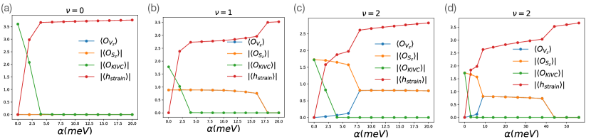
Figure S9: (a), (b), (c) Evolution of order parameters as a function of strain amplitude $\alpha$ at $\nu=0,-1,-2$. (d) Evolution of order parameters at $\nu=-2$ with an extended parameter region $0\text{meV}\leq\alpha\leq 55$meV

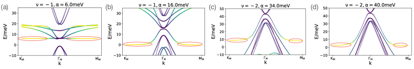
Figure S10: Band structure at $\nu=-1$ (a), (b) and $\nu=-2$ (c), (d). Red circles mark the relevant flat bands.

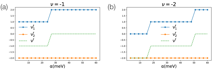
Figure S11: Evolution of filling as a function of the strain in the zero-hybridization model at $\nu=-1,-2$.

S5.5 Strain

We now discuss the derivation of strain term in the Eq. S95. Here we will take a minimal model to capture the effect of strain, and leave a detailed analysis (based on Ref. Vafek and Kang (2022)) for future study. We take the single-particle Hamiltonian of twisted bilayer graphene at valley $\eta$ and with non-zero strain Nakatsuji and Koshino (2022a)

$$H^{\eta}(\mathbf{k})=\begin{bmatrix}H^{\eta}_{1}(\mathbf{k})&U\\ U^{\dagger}&H^{\eta}_{2}(\mathbf{k})\end{bmatrix}$$ (S132)

where $H_{l}(\mathbf{k})$ is a $2\times 2$ matrix that characterizes the Hamiltonian of $l$-layer graphene. $U$ is the interlayer coupling matrix. In real space, $U$ takes the form of

$$U=\sum_{j=1}^{3}U_{j}e^{i\eta\bm{q}_{j}\cdot\mathbf{r}},\quad U_{j}=\begin{bmatrix}w_{0}&w_{1}e^{-i\eta 2(j-1)\pi/3}\\ w_{1}e^{i\eta 2(j-1)\pi/3}&w_{0}\end{bmatrix}$$

with $w_{0},w_{1}$ are two constant parameters that characterize the interlayer couplings. $H_{l}(\mathbf{k})$ is given by

$$H^{\eta}_{l=1,2}(\mathbf{k})=-\hbar v_{F}\bigg{[}\bigg{(}R(\mp\theta)+\mathcal{E}^{l}\bigg{)}^{-1}(\mathbf{k}+\frac{e}{\hbar}\bm{A}^{l,\eta})\bigg{]}\cdot\bm{\sigma}^{\eta}$$

where $\bm{\sigma}^{\eta}=(\eta\sigma_{x},\sigma_{y})$ , $R(\theta)$ is a rotation matrix, $\theta$ is the twist angle and Nakatsuji and Koshino (2022a)

$$\mathcal{E}^{l}=\begin{bmatrix}\epsilon_{xx}^{(l)}&-\Omega^{(l)}+\epsilon_{xy}^{(l)}\\ -\Omega^{(l)}+\epsilon_{xy}^{(l)}&\epsilon_{yy}^{(l)}\end{bmatrix}$$

$$\bm{A}^{l,\eta}=\eta\frac{3\beta\gamma_{0}}{2ev_{F}}\begin{bmatrix}\epsilon_{-}^{(l)}\\ \epsilon_{xy}^{(l)}\end{bmatrix},\quad\gamma_{0}=2.7\text{eV},\quad\beta\approx 3.14$$

$$\epsilon_{\pm}^{(l)}=\frac{1}{2}(\epsilon_{xx}^{(l)}\pm\epsilon_{yy}^{(l)})\,.$$ (S134)

$\epsilon_{xx}^{(l)},\epsilon_{yy}^{(l)}$ are normal strains along $x$ and $y$ directions respectively, $\epsilon_{xy}^{(l)}$ is the sheer strain. $\Omega^{(l)}$ denotes a rotation from the twist angles Nakatsuji and Koshino (2022a). Since the flat band is sensitive to $\epsilon_{-}=(\epsilon_{-}^{(1)}-\epsilon_{-}^{(2)})/2$ and $\epsilon_{xy}=(\epsilon_{xy}^{(1)}-\epsilon_{xy}^{(2)})/2$ Nakatsuji and Koshino (2022a), we consider the heterostrain with $\Omega^{(l)}=0,\epsilon_{+}^{(l)}=0,\epsilon_{-}^{(l)}=(-1)^{l+1}\epsilon_{-},\epsilon_{xy}^{(l)}=(-1)^{l+1}\epsilon_{xy}$. We further focus on the sheer strain $\epsilon_{xy}$ and set the normal anisotropic strain to be zero $\epsilon_{-}=0$. For small twist angle, we approximately have

$$H^{\eta}_{l=1,2}(\mathbf{k})\approx -\hbar v_{F}\bigg{[}\bigg{(}R(\pm\theta)-\mathcal{E}^{l}\bigg{)}(\mathbf{k}+\frac{e}{\hbar}\bm{A}^{l,\eta})\bigg{]}\cdot\bm{\sigma}^{\eta}$$

$$\approx -\hbar v_{F}\bigg{[}R(\pm\theta)\mathbf{k}-\mathcal{E}^{l}\mathbf{k}+\frac{e}{\hbar}\bm{A}^{l,\eta}\bigg{]}\cdot\bm{\sigma}^{\eta}$$ (S135)

The effect of strain is then captured by the following single particle Hamiltonian of valley $\eta$

$$H_{strain}^{\eta}(\mathbf{k})=H_{strain,1}^{\eta}+H_{strain,2}^{\eta}$$

$$H_{strain,1}^{\eta}=-\frac{3\beta\gamma_{0}\eta}{2}\epsilon_{xy}\begin{bmatrix}\sigma_{y}&\\ &-\sigma_{y}\end{bmatrix},\quad\quad H_{strain,2}^{\eta}=\hbar v_{F}\epsilon_{xy}\begin{bmatrix}\eta k_{y}\sigma_{x}+k_{x}\sigma_{y}\\ &-\eta k_{y}\sigma_{x}-k_{x}\sigma_{y}\end{bmatrix}$$ (S136)

We next project the $H_{strain}^{\eta}(\mathbf{k})$ to the Wannier basis of $f$-electrons. We take the following wavefunction of $f$ electrons at $\mathbf{R}$ with orbital $\alpha$, valley $\eta$ and spin $s$  Song and Bernevig (2022)

$$|W_{\mathbf{R},\alpha=1,\eta,s}\rangle=\sqrt{\frac{2\pi\lambda_{0}^{2}}{\Omega_{tot}}}\sum_{l=\pm}\sum_{\mathbf{k}}\sum_{\mathbf{Q}\in\mathcal{Q}_{l\eta}}e^{i\frac{\pi}{4}l\eta-i\mathbf{k}\cdot\mathbf{R}-\frac{1}{2}\lambda_{0}^{2}(\mathbf{k}-\mathbf{Q})^{2}}|\mathbf{k},\mathbf{Q},1,\eta,s\rangle$$

$$|W_{\mathbf{R},\alpha=2,\eta,s}\rangle=\sqrt{\frac{2\pi\lambda_{0}^{2}}{\Omega_{tot}}}\sum_{l=\pm}\sum_{\mathbf{k}}\sum_{\mathbf{Q}\in\mathcal{Q}_{l\eta}}e^{-i\frac{\pi}{4}l\eta-i\mathbf{k}\cdot\mathbf{R}-\frac{1}{2}\lambda_{0}^{2}(\mathbf{k}-\mathbf{Q})^{2}}|\mathbf{k},\mathbf{Q},2,\eta,s\rangle$$ (S137)

where $\lambda_{0}=0.1a_{M}$, $\Omega_{tot}$ is the total area of the sample and $\mathcal{Q}_{l\eta}=\{\pm\bm{q}_{1}+n_{1}\bm{b}_{M,1}+n_{2}\bm{b}_{M,2}|n_{1},n_{2}\in\mathbb{Z}\}$, $\bm{q}_{1}=k_{\theta}(0,-1)$ Song and Bernevig (2022). From Eq. S136 and Eq. S137, we can calculate

$$h^{strain}_{\alpha\eta s,\alpha_{2}\eta_{2}s_{2}}=\frac{1}{N_{M}}\sum_{\mathbf{R}}\langle W_{\mathbf{R},\alpha,\eta,s}|\sum_{\mathbf{k},\alpha^{\prime}l^{\prime},\alpha_{2}^{\prime}l_{2}^{\prime},\eta^{\prime},s^{\prime}}\psi^{\dagger}_{\mathbf{k},l,\alpha^{\prime},\eta^{\prime},s^{\prime}}[H_{strain}^{\eta^{\prime}}(\mathbf{k})]_{l^{\prime}\alpha^{\prime},l_{2}^{\prime}\alpha_{2}^{\prime}}\psi_{\mathbf{k},l_{2}^{\prime}\alpha^{\prime},\eta^{\prime},s^{\prime}}|W_{\mathbf{R},\alpha_{2},\eta_{2},s_{2}}\rangle$$ (S138)

where $\psi_{\mathbf{k},l,\alpha,\eta,s}$ is the electron operator of the original electron basis with momentum $\mathbf{k}$, layer $l$, sublattice $\alpha$, valley $\eta$ and spin $s$. Here, we take the average over all the moiré unit cells (sum over $\mathbf{R}$), and thus we only keep the momentum-independent (in $f$-electron basis) contributions. We leave the momentum-dependent term for future studies. In the $f$-basis, the strain can be characterized by

$${\hat{H}}_{strain}=\sum_{\mathbf{R},\alpha\eta s,\alpha_{2}\eta_{2}s_{2}}h^{strain}_{\alpha\eta s,\alpha_{2}\eta_{2}s_{2}}f_{\mathbf{R},\alpha\eta s}^{\dagger}f_{\mathbf{R},\alpha_{2}\eta_{2}s_{2}}$$ (S139)

We next evaluate $h^{strain}$ from Eq. S138. We separate $h^{strain}$ into two parts (Eq. S136)

$$h^{strain,1}_{\alpha\eta s,\alpha_{2}\eta_{2}s_{2}}=\frac{1}{N_{M}}\sum_{\mathbf{R}}\langle W_{\mathbf{R},\alpha,\eta,s}|\sum_{\mathbf{k},\alpha^{\prime}l^{\prime},\alpha_{2}^{\prime}l_{2}^{\prime},\eta^{\prime},s^{\prime}}\psi^{\dagger}_{\mathbf{k},l,\alpha^{\prime},\eta^{\prime},s^{\prime}}[H_{strain,1}^{\eta^{\prime}}(\mathbf{k})]_{l^{\prime}\alpha^{\prime},l_{2}^{\prime}\alpha_{2}^{\prime}}\psi_{\mathbf{k},l_{2}^{\prime}\alpha^{\prime},\eta^{\prime},s^{\prime}}|W_{\mathbf{R},\alpha_{2},\eta_{2},s_{2}}\rangle$$

$$h^{strain,2}_{\alpha\eta s,\alpha_{2}\eta_{2}s_{2}}=\frac{1}{N_{M}}\sum_{\mathbf{R}}\langle W_{\mathbf{R},\alpha,\eta,s}|\sum_{\mathbf{k},\alpha^{\prime}l^{\prime},\alpha_{2}^{\prime}l_{2}^{\prime},\eta^{\prime},s^{\prime}}\psi^{\dagger}_{\mathbf{k},l,\alpha^{\prime},\eta^{\prime},s^{\prime}}[H_{strain,2}^{\eta^{\prime}}(\mathbf{k})]_{l^{\prime}\alpha^{\prime},l_{2}^{\prime}\alpha_{2}^{\prime}}\psi_{\mathbf{k},l_{2}^{\prime}\alpha^{\prime},\eta^{\prime},s^{\prime}}|W_{\mathbf{R},\alpha_{2},\eta_{2},s_{2}}\rangle$$ (S140)

For $h^{strain,1}$, using Eq. S136, Eq. S137 and Eq. S140, we find

$$h^{strain,1}_{\alpha\eta s,\alpha_{2}\eta_{2}s_{2}}$$

$$= \delta_{\eta,\eta_{2}}\delta_{s,s_{2}}\delta_{\alpha,3-\alpha_{2}}\frac{2\pi\lambda_{0}^{2}}{\Omega_{tot}}\frac{-3\beta\gamma_{0}}{2}\epsilon_{xy}\sum_{l=\pm}\sum_{\mathbf{Q}\in\mathcal{Q}_{l\eta}}\sum_{\mathbf{k}}i(-1)^{\alpha}l\eta e^{-\lambda_{0}^{2}(\mathbf{k}-\mathbf{Q})^{2}}e^{-i\frac{\pi\eta l}{2}(-1)^{\alpha+1}}$$

$$= \delta_{\eta,\eta_{2}}\delta_{s,s_{2}}\delta_{\alpha,3-\alpha_{2}}\frac{3\pi\lambda_{0}^{2}\beta\gamma_{0}}{\Omega_{tot}}\epsilon_{xy}\sum_{\mathbf{k}}\bigg{[}\sum_{\mathbf{Q}\in\mathcal{Q}_{+}}e^{-\lambda_{0}^{2}(\mathbf{k}-\mathbf{Q})^{2}}+\sum_{\mathbf{Q}\in\mathcal{Q}_{-}}e^{-\lambda_{0}^{2}(\mathbf{k}-\mathbf{Q})^{2}}\bigg{]}$$ (S141)

In a more compact form, we find

$$h^{strain,1}=\alpha\sigma_{x}\tau_{0}\varsigma_{0}$$

$$\alpha=\frac{3\pi\lambda_{0}^{2}\beta\gamma_{0}}{\Omega_{tot}}\epsilon_{xy}\sum_{\mathbf{k}}\bigg{[}\sum_{\mathbf{Q}\in\mathcal{Q}_{+}}e^{-\lambda_{0}^{2}(\mathbf{k}-\mathbf{Q})^{2}}+\sum_{\mathbf{Q}\in\mathcal{Q}_{-}}e^{-\lambda_{0}^{2}(\mathbf{k}-\mathbf{Q})^{2}}\bigg{]}\approx\bigg{(}1.3\times 10^{4}\epsilon_{xy}\bigg{)}\text{meV}\,.$$ (S142)

We next calculate $h^{strain,2}$, using Eq. S136, Eq. S137 and Eq. S140, we find

$$h^{strain,2}_{\alpha\eta s,\alpha_{2}\eta_{2}s_{2}}$$

$$= \delta_{\eta,\eta_{2}}\delta_{s,s_{2}}\delta_{\alpha,3-\alpha_{2}}\frac{2\pi\lambda_{0}^{2}\hbar\epsilon_{xy}}{\Omega_{tot}}\sum_{l=\pm}\sum_{Q\in\mathcal{Q}_{l\eta}}\sum_{\mathbf{k}}l\bigg{(}\eta(k_{y}-Q_{y})+i(-1)^{\alpha}(k_{x}-Q_{x})\bigg{)}e^{i\frac{\pi}{2}l\eta(-1)^{\alpha}}e^{-\lambda_{0}^{2}(\mathbf{k}-\mathbf{Q})^{2}}$$

$$= \delta_{\eta,\eta_{2}}\delta_{s,s_{2}}\delta_{\alpha,3-\alpha_{2}}\frac{2\pi\lambda_{0}^{2}\hbar\epsilon_{xy}}{\Omega_{tot}}\sum_{\mathbf{k}}\bigg{[}\sum_{Q\in\mathcal{Q}_{\eta}}\bigg{(}\eta(k_{y}-Q_{y})+i(-1)^{\alpha}(k_{x}-Q_{x})\bigg{)}i\eta(-1)^{\alpha}e^{-\lambda_{0}^{2}(\mathbf{k}-\mathbf{Q})^{2}}$$

$$+\sum_{Q\in\mathcal{Q}_{-\eta}}\bigg{(}\eta(k_{y}-Q_{y})+i(-1)^{\alpha}(k_{x}-Q_{x})\bigg{)}i\eta(-1)^{\alpha}e^{-\lambda_{0}^{2}(\mathbf{k}-\mathbf{Q})^{2}}\bigg{]}$$

$$= \delta_{\eta,\eta_{2}}\delta_{s,s_{2}}\delta_{\alpha,3-\alpha_{2}}\frac{2\pi\lambda_{0}^{2}\hbar\epsilon_{xy}}{\Omega_{tot}}\sum_{\mathbf{k}}\sum_{\mathbf{Q}\in\mathcal{Q}_{0}}\bigg{(}\eta(k_{y}-Q_{y}-\eta q_{1,y})+i(-1)^{\alpha}(k_{x}-Q_{x}-\eta q_{1,x})\bigg{)}i\eta(-1)^{\alpha}e^{-\lambda_{0}^{2}(\mathbf{k}-\mathbf{Q}-\eta\mathbf{q}_{1})^{2}}$$

$$+\bigg{(}\eta(k_{y}-Q_{y}+\eta q_{1,y})+i(-1)^{\alpha}(k_{x}-Q_{x}+\eta q_{1,x})\bigg{)}i\eta(-1)^{\alpha}e^{-\lambda_{0}^{2}(\mathbf{k}-\mathbf{Q}+\eta\mathbf{q}_{1})^{2}}\bigg{]}$$ (S143)

where we let $\mathcal{Q}_{0}=\{n_{1}\bm{b}_{M,1}+n_{2}\bm{b}_{M,2}|n_{1},n_{2}\in\mathbb{Z}\}$. Since $\mathbf{q}_{1}=k_{\theta}(0,1)$, $q_{1,x}=0,q_{1,y}=k_{\theta}$, we find

$$h^{strain,2}_{\alpha\eta s,\alpha_{2}\eta_{2}s_{2}}$$

$$= \delta_{\eta,\eta_{2}}\delta_{s,s_{2}}\delta_{\alpha,3-\alpha_{2}}\frac{2\pi\lambda_{0}^{2}\hbar\epsilon_{xy}}{\Omega_{tot}}\sum_{\mathbf{k}}\sum_{\mathbf{Q}\in\mathcal{Q}_{0}}\bigg{[}i(-1)^{\alpha}(k_{y}-Q_{y})f_{+}(\mathbf{k}-\mathbf{Q})-iq_{1,y}(-1)^{\alpha}f_{-}(\mathbf{k}-\mathbf{Q})$$

$$-(k_{x}-Q_{x})\eta f_{+}(\mathbf{k}-\mathbf{Q})$$ (S144)

where we define

$$f_{\pm}(\mathbf{k}-\mathbf{Q})=\pm e^{-\lambda_{0}^{2}(\mathbf{k}-\mathbf{Q}+\mathbf{q}_{1})^{2}}+e^{-\lambda_{0}^{2}(\mathbf{k}-\mathbf{Q}-\mathbf{q}_{1})^{2}}$$ (S145)

Since $\mathbf{q}_{1}=k_{\theta}(0,1)$, $f_{+}(\mathbf{k}-\mathbf{Q})$ is an even function of both $(\mathbf{k}-\mathbf{Q})_{x}$ and $(\mathbf{k}-\mathbf{Q})_{y}$ and $f_{-}(\mathbf{k}-\mathbf{Q})$ is an even function of $(\mathbf{k}-\mathbf{Q})_{x}$ and an odd function of $(\mathbf{k}-\mathbf{Q})_{y}$. Therefore,

$$\sum_{\mathbf{k}}\sum_{\mathbf{Q}\in\mathcal{Q}_{0}}(k_{y}-Q_{y})f_{+}(\mathbf{k}-\mathbf{Q})=0,\quad\quad\sum_{\mathbf{k}}\sum_{\mathbf{Q}\in\mathcal{Q}_{0}}f_{-}(\mathbf{k}-\mathbf{Q})=0,\quad\quad \sum_{\mathbf{k}}\sum_{\mathbf{Q}\in\mathcal{Q}_{0}}(k_{x}-Q_{x})f_{+}(\mathbf{k}-\mathbf{Q})=0$$ (S146)

Thus,

$$h^{strain,2}_{\alpha\eta s,\alpha_{2}\eta_{2}s_{2}}=0$$ (S147)

However, we mention that, even though $h^{strain,2}=0$, $H_{strain,2}^{\eta}$ in Eq. S136 can contribute a $\mathbf{k}$-denpendent term in the THF model which has been omitted here.

Combining Eq. S142 and Eq. S147, we have

$${\hat{H}}_{strain}= \sum_{\mathbf{R},\alpha\eta s,\alpha_{2}\eta_{2}s_{2}}\alpha_{\alpha\eta s,\alpha_{2}\eta_{2}s_{2}}f_{\mathbf{R},\alpha\eta s}^{\dagger}f_{\mathbf{R},\alpha_{2}\eta_{2}s_{2}}= \alpha\sum_{\mathbf{R},\alpha\eta s,\alpha_{2}\eta_{2}s_{2}}[h_{strain}]_{\alpha\eta s,\alpha_{2}\eta_{2}s_{2}}f_{\mathbf{R},\alpha\eta s}^{\dagger}f_{\mathbf{R},\alpha_{2}\eta_{2}s_{2}}$$ (S148)

which is equivalent to the Eq. S95. $\alpha$ is connected to $\epsilon_{xy}$ via

$$\alpha=\frac{3\pi\lambda_{0}^{2}\beta\gamma_{0}}{\Omega_{tot}}\epsilon_{xy}\sum_{\mathbf{k}}\bigg{[}\sum_{\mathbf{Q}\in\mathcal{Q}_{+}}e^{-\lambda_{0}^{2}(\mathbf{k}-\mathbf{Q})^{2}}+\sum_{\mathbf{Q}\in\mathcal{Q}_{-}}e^{-\lambda_{0}^{2}(\mathbf{k}-\mathbf{Q})^{2}}\bigg{]}\approx\bigg{(}1.3\times 10^{4}\epsilon_{xy}\bigg{)}\text{meV}\,.$$ (S149)

For a typical strain at the order of $\epsilon_{xy}\sim 10^{-3}$ Nakatsuji and Koshino (2022a), $\alpha\sim 13$meV. We mention that the strain could also induce addition terms to the conduction $c$-electron blocks ($c^{\dagger}c$) and $f$-$c$ hybridization blocks ($c^{\dagger}f,f^{\dagger}c$), which are expected to be small. Here, we only consider a minimal model, that is zeroth order in $\mathbf{k}$, to capture the essential effect of the strain. We leave a comprehensive construction of strain term (based on Ref. Vafek and Kang (2022)) for future study.

S6 Dynamical mean field theory: implementation

We study dynamical effects of the $f$-$f$ density-density term using DMFT. The $c$-$f$ and $c$-$c$ density terms are included in this model on the Hartree level. We neglect the $f$-$c$ exchange interaction $\hat{H}_{J}$. We treat a Hamiltonian of the form $\hat{H}_{c}+\hat{H}_{fc}+\hat{H}_{U}+\hat{H}^{MF}_{W}+\hat{H}^{MF}_{V}$ where the first two terms compose the non-interacting THF model and the remaining terms are given by

$$\hat{H}_{U}= \frac{U}{2}\sum_{(\alpha,\eta,\sigma)\neq(\alpha^{\prime},\eta^{\prime},\sigma^{\prime})}f^{\dagger}_{\alpha,\eta,\sigma}f_{\alpha,\eta,\sigma}f^{\dagger}_{\alpha^{\prime},\eta^{\prime},\sigma^{\prime}}f_{\alpha^{\prime},\eta^{\prime},\sigma^{\prime}}$$

$$-3.5U\sum_{(\alpha,\eta,\sigma)}f^{\dagger}_{\alpha,\eta,\sigma}f_{\alpha,\eta,\sigma}$$ (S150)

$$\hat{H}^{MF}_{W}= W\nu_{f}\sum_{(a,\eta,\sigma)}c^{\dagger}_{a,\eta,\sigma}c_{a,\eta,\sigma}+W\nu_{c}\sum_{(\alpha,\eta,\sigma)}f_{\alpha,\eta,\sigma}^{\dagger}f_{\alpha,\eta,\sigma},$$ (S151)

$$\hat{H}^{MF}_{V}= V\nu_{c}\sum_{(a,\eta,\sigma)}c^{\dagger}_{a,\eta,\sigma}c_{a,\eta,\sigma}.$$ (S152)

Here, the last two terms are mean-field decoupled and therefore composed of single particle terms, and we have neglected all constant terms as an overall shift does not affect the observables we are interested in. The two particle term $\hat{H}_{U}$ is restricted to the f- subspace. We proceed with an LDA+DMFT-style calculation with a correlated subspace made up of f- electrons embedded in a larger space of f- and c- electrons. By allowing an arbitrary shift of the chemical potential $\mu$ and fixing the total filling $\nu=\nu_{f}+\nu_{c}$, we can consider an effective interacting Hamiltonian restricted to the the f- subspace:

$$\hat{H}^{eff}_{I}= \hat{H}_{ff}+\hat{H}_{DC}$$ (S153)

$$\hat{H}_{ff}= \frac{U}{2}\sum_{(\alpha,\eta,\sigma)\neq(\alpha^{\prime},\eta^{\prime},\sigma^{\prime})}f^{\dagger}_{\alpha,\eta,\sigma}f_{\alpha,\eta,\sigma}f^{\dagger}_{\alpha^{\prime},\eta^{\prime},\sigma^{\prime}}f_{\alpha^{\prime},\eta^{\prime},\sigma^{\prime}}$$ (S154)

$$\hat{H}_{DC}= \underbrace{\left(-3.5U+(\nu-2\nu_{f})W-V(\nu-\nu_{f})\right)}_{\mu_{DC}(\nu_{f})}\sum_{(\alpha,\eta,\sigma)}f^{\dagger}_{\alpha,\eta,\sigma}f_{\alpha,\eta,\sigma}.$$ (S155)

The $f$-electron occupation $\nu_{f}$ is self-consistently calculated along with the the $f$- subspace self-energy $\Sigma_{f}$ in at each step of the DMFT loop for a set of different total fillings ($\nu$) and temperatures (T). Written in this way, the single particle terms can be treated as an iteration-dependent double counting potential, $\mu^{(i)}_{DC}=\mu_{DC}\left(\nu_{f}^{(i)}\right)$, where the superscript labels the iteration number.

In the $i$th iteration of the self-consistency loop, we perform the following sequence of steps:

1. Embed the old impurity self-energy $\Sigma_{f}^{(i-1)}$ into the lattice Green’s function associated to the Hamiltonian $\hat{H}_{c}+\hat{H}_{fc}+\hat{H}_{DC}^{(i-1)}$.

2. Fix the total filling to $\nu$.

3. Calculate the new orbital-resolved fillings $\nu_{f}^{(i)}$ and $\nu_{c}^{(i)}$.

4. Determine the new double counting term $\mu_{DC}^{(i)}$.

5. Use a CT-QMC solver to obtain the new self energy $\Sigma_{f}^{(i)}$.

We performed our calculations in parallel using the w2dynamics suite Parragh et al. (2012); Wallerberger et al. (2019) as well as the TRIQS family of packages Parcollet et al. (2015); Seth et al. (2016); Aichhorn et al. (2016).

In Fig. 3(a) of the main text, the zero frequency spectral weight and the scattering rate are computed by extrapolating the green function and the self-energy respectively on the Matsubara axis. We approximate these by using the value at the first Matsubara frequency so that

$$\Gamma =-\text{Im}\Sigma(\omega=0)\approx-\text{Im}\Sigma(\omega_{0}),$$ (S156)

$$A(\omega=0) =-\frac{1}{\pi}\left(\sum_{k}\text{Tr}G(k,\omega=0)\right)\approx-\frac{1}{\pi}\left(\sum_{k}\text{Tr}G(k,\omega_{0})\right).$$ (S157)

References

• Song and Bernevig (2022) Zhi-Da Song and B. Andrei Bernevig, “Magic-angle twisted bilayer graphene as a topological heavy fermion problem,” Phys. Rev. Lett. 129, 047601 (2022).
• (2) Haoyu Hu, B. Andrei Bernevig,  and Alexei M. Tsvelik, to be published .
• Coleman (2015) Piers Coleman, Introduction to many-body physics (Cambridge University Press, 2015).
• Bistritzer and MacDonald (2011) Rafi Bistritzer and Allan H MacDonald, “Moiré bands in twisted double-layer graphene,” Proceedings of the National Academy of Sciences 108, 12233–12237 (2011).
• Balents et al. (2020a) Leon Balents, Cory R. Dean, Dmitri K. Efetov,  and Andrea F. Young, “Superconductivity and strong correlations in moiré flat bands,” Nature Physics 16, 725–733 (2020a).
• Andrei et al. (2021) Eva Y. Andrei, Dmitri K. Efetov, Pablo Jarillo-Herrero, Allan H. MacDonald, Kin Fai Mak, T. Senthil, Emanuel Tutuc, Ali Yazdani,  and Andrea F. Young, “The marvels of moiré materials,” Nature Reviews Materials 6, 201–206 (2021).
• Cao et al. (2020a) Yuan Cao, Debanjan Chowdhury, Daniel Rodan-Legrain, Oriol Rubies-Bigorda, Kenji Watanabe, Takashi Taniguchi, T. Senthil,  and Pablo Jarillo-Herrero, “Strange metal in magic-angle graphene with near planckian dissipation,” Phys. Rev. Lett. 124, 076801 (2020a).
• Lu et al. (2019) Xiaobo Lu, Petr Stepanov, Wei Yang, Ming Xie, Mohammed Ali Aamir, Ipsita Das, Carles Urgell, Kenji Watanabe, Takashi Taniguchi, Guangyu Zhang, Adrian Bachtold, Allan H. MacDonald,  and Dmitri K. Efetov, “Superconductors, orbital magnets and correlated states in magic-angle bilayer graphene,” Nature 574, 653–657 (2019).
• Stepanov et al. (2020) Petr Stepanov, Ipsita Das, Xiaobo Lu, Ali Fahimniya, Kenji Watanabe, Takashi Taniguchi, Frank H. L. Koppens, Johannes Lischner, Leonid Levitov,  and Dmitri K. Efetov, “Untying the insulating and superconducting orders in magic-angle graphene,” Nature 583, 375–378 (2020).
• Xie and MacDonald (2021) Ming Xie and A. H. MacDonald, “Weak-Field Hall Resistivity and Spin-Valley Flavor Symmetry Breaking in Magic-Angle Twisted Bilayer Graphene,” Phys. Rev. Lett. 127, 196401 (2021).
• Kerelsky et al. (2019) Alexander Kerelsky, Leo J. McGilly, Dante M. Kennes, Lede Xian, Matthew Yankowitz, Shaowen Chen, K. Watanabe, T. Taniguchi, James Hone, Cory Dean, Angel Rubio,  and Abhay N. Pasupathy, “Maximized electron interactions at the magic angle in twisted bilayer graphene,” Nature 572, 95–100 (2019).
• Jiang et al. (2019) Yuhang Jiang, Xinyuan Lai, Kenji Watanabe, Takashi Taniguchi, Kristjan Haule, Jinhai Mao,  and Eva Y. Andrei, “Charge order and broken rotational symmetry in magic-angle twisted bilayer graphene,” Nature 573, 91–95 (2019).
• Wong et al. (2020) Dillon Wong, Kevin P. Nuckolls, Myungchul Oh, Biao Lian, Yonglong Xie, Sangjun Jeon, Kenji Watanabe, Takashi Taniguchi, B. Andrei Bernevig,  and Ali Yazdani, “Cascade of electronic transitions in magic-angle twisted bilayer graphene,” Nature 582, 198–202 (2020).
• Zondiner et al. (2020) U. Zondiner, A. Rozen, D. Rodan-Legrain, Y. Cao, R. Queiroz, T. Taniguchi, K. Watanabe, Y. Oreg, F. von Oppen, Ady Stern, E. Berg, P. Jarillo-Herrero,  and S. Ilani, “Cascade of phase transitions and Dirac revivals in magic-angle graphene,” Nature 582, 203–208 (2020).
• Choi et al. (2021) Youngjoon Choi, Hyunjin Kim, Yang Peng, Alex Thomson, Cyprian Lewandowski, Robert Polski, Yiran Zhang, Harpreet Singh Arora, Kenji Watanabe, Takashi Taniguchi, Jason Alicea,  and Stevan Nadj-Perge, “Correlation-driven topological phases in magic-angle twisted bilayer graphene,” Nature 589, 536–541 (2021).
• Park et al. (2021) Jeong Min Park, Yuan Cao, Kenji Watanabe, Takashi Taniguchi,  and Pablo Jarillo-Herrero, “Flavour Hund’s coupling, Chern gaps and charge diffusivity in moiré graphene,” Nature 592, 43–48 (2021).
• Lu et al. (2021) Xiaobo Lu, Biao Lian, Gaurav Chaudhary, Benjamin A. Piot, Giulio Romagnoli, Kenji Watanabe, Takashi Taniguchi, Martino Poggio, Allan H. MacDonald, B. Andrei Bernevig,  and Dmitri K. Efetov, “Multiple flat bands and topological Hofstadter butterfly in twisted bilayer graphene close to the second magic angle,” PNAS 118 (2021), 10.1073/pnas.2100006118.
• Saito et al. (2021a) Yu Saito, Fangyuan Yang, Jingyuan Ge, Xiaoxue Liu, Takashi Taniguchi, Kenji Watanabe, J. I. A. Li, Erez Berg,  and Andrea F. Young, “Isospin pomeranchuk effect in twisted bilayer graphene,” Nature 592, 220–224 (2021a).
• Rozen et al. (2021) Asaf Rozen, Jeong Min Park, Uri Zondiner, Yuan Cao, Daniel Rodan-Legrain, Takashi Taniguchi, Kenji Watanabe, Yuval Oreg, Ady Stern, Erez Berg, Pablo Jarillo-Herrero,  and Shahal Ilani, “Entropic evidence for a Pomeranchuk effect in magic-angle graphene,” Nature 592, 214–219 (2021).
• Das et al. (2022) Ipsita Das, Cheng Shen, Alexandre Jaoui, Jonah Herzog-Arbeitman, Aaron Chew, Chang-Woo Cho, Kenji Watanabe, Takashi Taniguchi, Benjamin A. Piot, B. Andrei Bernevig,  and Dmitri K. Efetov, “Observation of reentrant correlated insulators and interaction-driven fermi-surface reconstructions at one magnetic flux quantum per moiré unit cell in magic-angle twisted bilayer graphene,” Phys. Rev. Lett. 128, 217701 (2022).
• Seifert et al. (2020) Paul Seifert, Xiaobo Lu, Petr Stepanov, José Ramón Durán Retamal, John N. Moore, Kin-Chung Fong, Alessandro Principi,  and Dmitri K. Efetov, “Magic-angle bilayer graphene nanocalorimeters: Toward broadband, energy-resolving single photon detection,” Nano Letters 20, 3459–3464 (2020).
• Otteneder et al. (2020) Maximilian Otteneder, Stefan Hubmann, Xiaobo Lu, Dmitry A. Kozlov, Leonid E. Golub, Kenji Watanabe, Takashi Taniguchi, Dmitri K. Efetov,  and Sergey D. Ganichev, “Terahertz photogalvanics in twisted bilayer graphene close to the second magic angle,” Nano Letters 20, 7152–7158 (2020).
• Lisi et al. (2021) Simone Lisi, Xiaobo Lu, Tjerk Benschop, Tobias A. de Jong, Petr Stepanov, Jose R. Duran, Florian Margot, Irène Cucchi, Edoardo Cappelli, Andrew Hunter, Anna Tamai, Viktor Kandyba, Alessio Giampietri, Alexei Barinov, Johannes Jobst, Vincent Stalman, Maarten Leeuwenhoek, Kenji Watanabe, Takashi Taniguchi, Louk Rademaker, Sense Jan van der Molen, Milan P. Allan, Dmitri K. Efetov,  and Felix Baumberger, “Observation of flat bands in twisted bilayer graphene,” Nature Physics 17, 189–193 (2021).
• Benschop et al. (2021) Tjerk Benschop, Tobias A. de Jong, Petr Stepanov, Xiaobo Lu, Vincent Stalman, Sense Jan van der Molen, Dmitri K. Efetov,  and Milan P. Allan, “Measuring local moiré lattice heterogeneity of twisted bilayer graphene,” Phys. Rev. Res. 3, 013153 (2021).
• Hesp et al. (2021) Niels C. H. Hesp, Iacopo Torre, Daniel Rodan-Legrain, Pietro Novelli, Yuan Cao, Stephen Carr, Shiang Fang, Petr Stepanov, David Barcons-Ruiz, Hanan Herzig Sheinfux, Kenji Watanabe, Takashi Taniguchi, Dmitri K. Efetov, Efthimios Kaxiras, Pablo Jarillo-Herrero, Marco Polini,  and Frank H. L. Koppens, “Observation of interband collective excitations in twisted bilayer graphene,” Nature Physics 17, 1162–1168 (2021).
• Hubmann et al. (2022) S. Hubmann, P. Soul, G. Di Battista, M. Hild, K. Watanabe, T. Taniguchi, D. K. Efetov,  and S. D. Ganichev, “Nonlinear intensity dependence of photogalvanics and photoconductance induced by terahertz laser radiation in twisted bilayer graphene close to magic angle,” Phys. Rev. Mater. 6, 024003 (2022).
• Jaoui et al. (2022) Alexandre Jaoui, Ipsita Das, Giorgio Di Battista, Jaime Díez-Mérida, Xiaobo Lu, Kenji Watanabe, Takashi Taniguchi, Hiroaki Ishizuka, Leonid Levitov,  and Dmitri K. Efetov, “Quantum critical behaviour in magic-angle twisted bilayer graphene,” Nature Physics 18, 633–638 (2022).
• Grover et al. (2022) Sameer Grover, Matan Bocarsly, Aviram Uri, Petr Stepanov, Giorgio Di Battista, Indranil Roy, Jiewen Xiao, Alexander Y. Meltzer, Yuri Myasoedov, Keshav Pareek, Kenji Watanabe, Takashi Taniguchi, Binghai Yan, Ady Stern, Erez Berg, Dmitri K. Efetov,  and Eli Zeldov, “Chern mosaic and berry-curvature magnetism in magic-angle graphene,” Nature Physics 18, 885–892 (2022).
• Cao et al. (2018a) Yuan Cao, Valla Fatemi, Ahmet Demir, Shiang Fang, Spencer L. Tomarken, Jason Y. Luo, Javier D. Sanchez-Yamagishi, Kenji Watanabe, Takashi Taniguchi, Efthimios Kaxiras, Ray C. Ashoori,  and Pablo Jarillo-Herrero, “Correlated insulator behaviour at half-filling in magic-angle graphene superlattices,” Nature 556, 80–84 (2018a).
• Cao et al. (2020b) Yuan Cao, Daniel Rodan-Legrain, Oriol Rubies-Bigorda, Jeong Min Park, Kenji Watanabe, Takashi Taniguchi,  and Pablo Jarillo-Herrero, “Tunable correlated states and spin-polarized phases in twisted bilayer–bilayer graphene,” Nature 583, 215–220 (2020b).
• Polshyn et al. (2019) Hryhoriy Polshyn, Matthew Yankowitz, Shaowen Chen, Yuxuan Zhang, K. Watanabe, T. Taniguchi, Cory R. Dean,  and Andrea F. Young, “Large linear-in-temperature resistivity in twisted bilayer graphene,” Nat. Phys. 15, 1011–1016 (2019).
• Liu et al. (2021a) Xiaoxue Liu, Zhi Wang, K. Watanabe, T. Taniguchi, Oskar Vafek,  and J. I. A. Li, “Tuning electron correlation in magic-angle twisted bilayer graphene using Coulomb screening,” Science 371, 1261–1265 (2021a).
• Xie et al. (2019) Yonglong Xie, Biao Lian, Berthold Jäck, Xiaomeng Liu, Cheng-Li Chiu, Kenji Watanabe, Takashi Taniguchi, B. Andrei Bernevig,  and Ali Yazdani, “Spectroscopic signatures of many-body correlations in magic-angle twisted bilayer graphene,” Nature 572, 101–105 (2019).
• Choi et al. (2019) Youngjoon Choi, Jeannette Kemmer, Yang Peng, Alex Thomson, Harpreet Arora, Robert Polski, Yiran Zhang, Hechen Ren, Jason Alicea, Gil Refael, Felix von Oppen, Kenji Watanabe, Takashi Taniguchi,  and Stevan Nadj-Perge, “Electronic correlations in twisted bilayer graphene near the magic angle,” Nat. Phys. 15, 1174–1180 (2019).
• Nuckolls et al. (2020) Kevin P. Nuckolls, Myungchul Oh, Dillon Wong, Biao Lian, Kenji Watanabe, Takashi Taniguchi, B. Andrei Bernevig,  and Ali Yazdani, “Strongly correlated Chern insulators in magic-angle twisted bilayer graphene,” Nature 588, 610–615 (2020).
• Saito et al. (2021b) Yu Saito, Jingyuan Ge, Louk Rademaker, Kenji Watanabe, Takashi Taniguchi, Dmitry A. Abanin,  and Andrea F. Young, “Hofstadter subband ferromagnetism and symmetry-broken Chern insulators in twisted bilayer graphene,” Nat. Phys. , 1–4 (2021b).
• Das et al. (2021) Ipsita Das, Xiaobo Lu, Jonah Herzog-Arbeitman, Zhi-Da Song, Kenji Watanabe, Takashi Taniguchi, B. Andrei Bernevig,  and Dmitri K. Efetov, “Symmetry-broken Chern insulators and Rashba-like Landau-level crossings in magic-angle bilayer graphene,” Nat. Phys. 17, 710–714 (2021).
• Wu et al. (2021) Shuang Wu, Zhenyuan Zhang, K. Watanabe, T. Taniguchi,  and Eva Y. Andrei, “Chern insulators, van Hove singularities and topological flat bands in magic-angle twisted bilayer graphene,” Nat. Mater. 20, 488–494 (2021).
• Stepanov et al. (2021) Petr Stepanov, Ming Xie, Takashi Taniguchi, Kenji Watanabe, Xiaobo Lu, Allan H. MacDonald, B. Andrei Bernevig,  and Dmitri K. Efetov, “Competing zero-field chern insulators in superconducting twisted bilayer graphene,” Phys. Rev. Lett. 127, 197701 (2021).
• Cao et al. (2018b) Yuan Cao, Valla Fatemi, Shiang Fang, Kenji Watanabe, Takashi Taniguchi, Efthimios Kaxiras,  and Pablo Jarillo-Herrero, “Unconventional superconductivity in magic-angle graphene superlattices,” Nature 556, 43–50 (2018b).
• Cao et al. (2021) Yuan Cao, Daniel Rodan-Legrain, Jeong Min Park, Noah F. Q. Yuan, Kenji Watanabe, Takashi Taniguchi, Rafael M. Fernandes, Liang Fu,  and Pablo Jarillo-Herrero, “Nematicity and competing orders in superconducting magic-angle graphene,” Science 372, 264–271 (2021).
• Yankowitz et al. (2019) Matthew Yankowitz, Shaowen Chen, Hryhoriy Polshyn, Yuxuan Zhang, K. Watanabe, T. Taniguchi, David Graf, Andrea F. Young,  and Cory R. Dean, “Tuning superconductivity in twisted bilayer graphene,” Science 363, 1059–1064 (2019).
• Diez-Merida et al. (2021) Jaime Diez-Merida, Andrés Díez-Carlón, SY Yang, Y-M Xie, X-J Gao, Kenji Watanabe, Takashi Taniguchi, Xiaobo Lu, Kam Tuen Law,  and Dmitri K Efetov, “Magnetic josephson junctions and superconducting diodes in magic angle twisted bilayer graphene,” arXiv preprint arXiv:2110.01067  (2021).
• Di Battista et al. (2022) Giorgio Di Battista, Paul Seifert, Kenji Watanabe, Takashi Taniguchi, Kin Chung Fong, Alessandro Principi,  and Dmitri K. Efetov, “Revealing the thermal properties of superconducting magic-angle twisted bilayer graphene,” Nano Letters 22, 6465–6470 (2022).
• Efimkin and MacDonald (2018) Dmitry K. Efimkin and Allan H. MacDonald, “Helical network model for twisted bilayer graphene,” Phys. Rev. B 98, 035404 (2018).
• Vafek and Kang (2020) Oskar Vafek and Jian Kang, “Renormalization Group Study of Hidden Symmetry in Twisted Bilayer Graphene with Coulomb Interactions,” Phys. Rev. Lett. 125, 257602 (2020).
• Padhi et al. (2018) Bikash Padhi, Chandan Setty,  and Philip W. Phillips, “Doped Twisted Bilayer Graphene near Magic Angles: Proximity to Wigner Crystallization, Not Mott Insulation,” Nano Letters 18, 6175–6180 (2018)arXiv:1804.01101 [cond-mat.str-el] .
• Padhi et al. (2020) Bikash Padhi, Apoorv Tiwari, Titus Neupert,  and Shinsei Ryu, “Transport across twist angle domains in moir\’e graphene,” Phys. Rev. Research 2, 033458 (2020).
• Guinea and Walet (2018) Francisco Guinea and Niels R. Walet, “Electrostatic effects, band distortions, and superconductivity in twisted graphene bilayers,” PNAS 115, 13174–13179 (2018).
• Dodaro et al. (2018) J. F. Dodaro, S. A. Kivelson, Y. Schattner, X. Q. Sun,  and C. Wang, “Phases of a phenomenological model of twisted bilayer graphene,” Phys. Rev. B 98, 075154 (2018).
• Hejazi et al. (2021) Kasra Hejazi, Xiao Chen,  and Leon Balents, “Hybrid Wannier Chern bands in magic angle twisted bilayer graphene and the quantized anomalous Hall effect,” Physical Review Research 3, 013242 (2021), publisher: American Physical Society.
• Khalaf et al. (2021) Eslam Khalaf, Shubhayu Chatterjee, Nick Bultinck, Michael P. Zaletel,  and Ashvin Vishwanath, “Charged skyrmions and topological origin of superconductivity in magic-angle graphene,” Science Advances 7, eabf5299 (2021).
• Po et al. (2018) Hoi Chun Po, Liujun Zou, Ashvin Vishwanath,  and T. Senthil, “Origin of mott insulating behavior and superconductivity in twisted bilayer graphene,” Phys. Rev. X 8, 031089 (2018).
• König et al. (2020) E. J. König, Piers Coleman,  and A. M. Tsvelik, “Spin magnetometry as a probe of stripe superconductivity in twisted bilayer graphene,” Phys. Rev. B 102, 104514 (2020).
• Christos et al. (2020) Maine Christos, Subir Sachdev,  and Mathias S. Scheurer, “Superconductivity, correlated insulators, and Wess–Zumino–Witten terms in twisted bilayer graphene,” PNAS 117, 29543–29554 (2020).
• Kennes et al. (2018) Dante M. Kennes, Johannes Lischner,  and Christoph Karrasch, “Strong correlations and $d+\mathit{id}$ superconductivity in twisted bilayer graphene,” Phys. Rev. B 98, 241407 (2018).
• Huang et al. (2020) Yixuan Huang, Pavan Hosur,  and Hridis K. Pal, “Quasi-flat-band physics in a two-leg ladder model and its relation to magic-angle twisted bilayer graphene,” Phys. Rev. B 102, 155429 (2020).
• Guo et al. (2018) Huaiming Guo, Xingchuan Zhu, Shiping Feng,  and Richard T. Scalettar, “Pairing symmetry of interacting fermions on a twisted bilayer graphene superlattice,” Phys. Rev. B 97, 235453 (2018).
• Cha et al. (2021) Peter Cha, Aavishkar A. Patel,  and Eun-Ah Kim, “Strange metals from melting correlated insulators in twisted bilayer graphene,” Phys. Rev. Lett. 127, 266601 (2021).
• Kang et al. (2021) Jian Kang, B. Andrei Bernevig,  and Oskar Vafek, “Cascades between light and heavy fermions in the normal state of magic angle twisted bilayer graphene,” arXiv:2104.01145 [cond-mat]  (2021), arXiv:2104.01145 [cond-mat] .
• Wu et al. (2019) Xiao-Chuan Wu, Chao-Ming Jian,  and Cenke Xu, “Coupled-wire description of the correlated physics in twisted bilayer graphene,” Phys. Rev. B 99, 161405 (2019).
• Balents et al. (2020b) Leon Balents, Cory R. Dean, Dmitri K. Efetov,  and Andrea F. Young, “Superconductivity and strong correlations in moiré flat bands,” Nat. Phys. 16, 725–733 (2020b).
• Fernandes and Venderbos (2020) Rafael M. Fernandes and Jörn W. F. Venderbos, “Nematicity with a twist: Rotational symmetry breaking in a moiré superlattice,” Science Advances 6, eaba8834 (2020).
• Wilson et al. (2020) Justin H. Wilson, Yixing Fu, S. Das Sarma,  and J. H. Pixley, “Disorder in twisted bilayer graphene,” Phys. Rev. Research 2, 023325 (2020).
• Cea et al. (2019) Tommaso Cea, Niels R. Walet,  and Francisco Guinea, “Twists and the Electronic Structure of Graphitic Materials,” Nano Lett. 19, 8683–8689 (2019).
• Yu et al. (2022) Jiachen Yu, Benjamin A. Foutty, Zhaoyu Han, Mark E. Barber, Yoni Schattner, Kenji Watanabe, Takashi Taniguchi, Philip Phillips, Zhi-Xun Shen, Steven A. Kivelson,  and Benjamin E. Feldman, “Correlated hofstadter spectrum and flavour phase diagram in magic-angle twisted bilayer graphene,” Nature Physics 18, 825–831 (2022).
• Herzog-Arbeitman et al. (2020) Jonah Herzog-Arbeitman, Zhi-Da Song, Nicolas Regnault,  and B. Andrei Bernevig, “Hofstadter topology: Noncrystalline topological materials at high flux,” Phys. Rev. Lett. 125, 236804 (2020).
• Herzog-Arbeitman et al. (2022) Jonah Herzog-Arbeitman, Aaron Chew, Dmitri K. Efetov,  and B. Andrei Bernevig, “Reentrant correlated insulators in twisted bilayer graphene at 25 t ($2\pi$ flux),” Phys. Rev. Lett. 129, 076401 (2022).
• (69) Jiabin Yu, Ming Xie, B. Andrei Bernevig,  and Sankar Das Sarma, to be published .
• Kang and Vafek (2019) Jian Kang and Oskar Vafek, “Strong Coupling Phases of Partially Filled Twisted Bilayer Graphene Narrow Bands,” Phys. Rev. Lett. 122, 246401 (2019).
• Kang and Vafek (2018) Jian Kang and Oskar Vafek, “Symmetry, Maximally Localized Wannier States, and a Low-Energy Model for Twisted Bilayer Graphene Narrow Bands,” Phys. Rev. X 8, 031088 (2018).
• Koshino et al. (2018) Mikito Koshino, Noah F. Q. Yuan, Takashi Koretsune, Masayuki Ochi, Kazuhiko Kuroki,  and Liang Fu, “Maximally Localized Wannier Orbitals and the Extended Hubbard Model for Twisted Bilayer Graphene,” Phys. Rev. X 8, 031087 (2018).
• Ochi et al. (2018) Masayuki Ochi, Mikito Koshino,  and Kazuhiko Kuroki, “Possible correlated insulating states in magic-angle twisted bilayer graphene under strongly competing interactions,” Phys. Rev. B 98, 081102 (2018).
• Vafek and Kang (2021) Oskar Vafek and Jian Kang, “Lattice model for the coulomb interacting chiral limit of magic-angle twisted bilayer graphene: Symmetries, obstructions, and excitations,” Phys. Rev. B 104, 075143 (2021).
• Xu and Balents (2018) Cenke Xu and Leon Balents, “Topological Superconductivity in Twisted Multilayer Graphene,” Phys. Rev. Lett. 121, 087001 (2018).
• Xu et al. (2018) Xiao Yan Xu, K. T. Law,  and Patrick A. Lee, “Kekul\’e valence bond order in an extended Hubbard model on the honeycomb lattice with possible applications to twisted bilayer graphene,” Phys. Rev. B 98, 121406 (2018).
• Venderbos and Fernandes (2018) Jörn W. F. Venderbos and Rafael M. Fernandes, “Correlations and electronic order in a two-orbital honeycomb lattice model for twisted bilayer graphene,” Phys. Rev. B 98, 245103 (2018).
• Yuan and Fu (2018) Noah F. Q. Yuan and Liang Fu, “Model for the metal-insulator transition in graphene superlattices and beyond,” Phys. Rev. B 98, 045103 (2018).
• Da Liao et al. (2019) Yuan Da Liao, Zi Yang Meng,  and Xiao Yan Xu, “Valence Bond Orders at Charge Neutrality in a Possible Two-Orbital Extended Hubbard Model for Twisted Bilayer Graphene,” Phys. Rev. Lett. 123, 157601 (2019).
• Da Liao et al. (2021) Yuan Da Liao, Jian Kang, Clara N. Breiø, Xiao Yan Xu, Han-Qing Wu, Brian M. Andersen, Rafael M. Fernandes,  and Zi Yang Meng, “Correlation-Induced Insulating Topological Phases at Charge Neutrality in Twisted Bilayer Graphene,” Phys. Rev. X 11, 011014 (2021).
• Chichinadze et al. (2020) Dmitry V. Chichinadze, Laura Classen,  and Andrey V. Chubukov, “Nematic superconductivity in twisted bilayer graphene,” Phys. Rev. B 101, 224513 (2020).
• Seo et al. (2019) Kangjun Seo, Valeri N. Kotov,  and Bruno Uchoa, “Ferromagnetic Mott state in Twisted Graphene Bilayers at the Magic Angle,” Phys. Rev. Lett. 122, 246402 (2019).
• Liu et al. (2019a) Jianpeng Liu, Junwei Liu,  and Xi Dai, “Pseudo Landau level representation of twisted bilayer graphene: Band topology and implications on the correlated insulating phase,” Phys. Rev. B 99, 155415 (2019a).
• Zou et al. (2018) Liujun Zou, Hoi Chun Po, Ashvin Vishwanath,  and T. Senthil, “Band structure of twisted bilayer graphene: Emergent symmetries, commensurate approximants, and Wannier obstructions,” Phys. Rev. B 98, 085435 (2018).
• Song et al. (2019) Zhida Song, Zhijun Wang, Wujun Shi, Gang Li, Chen Fang,  and B. Andrei Bernevig, “All magic angles in twisted bilayer graphene are topological,” Phys. Rev. Lett. 123, 036401 (2019).
• Po et al. (2019) Hoi Chun Po, Liujun Zou, T. Senthil,  and Ashvin Vishwanath, “Faithful tight-binding models and fragile topology of magic-angle bilayer graphene,” Phys. Rev. B 99, 195455 (2019).
• Lian et al. (2020) Biao Lian, Fang Xie,  and B. Andrei Bernevig, “Landau level of fragile topology,” Phys. Rev. B 102, 041402 (2020).
• Hejazi et al. (2019a) Kasra Hejazi, Chunxiao Liu,  and Leon Balents, “Landau levels in twisted bilayer graphene and semiclassical orbits,” Phys. Rev. B 100, 035115 (2019a).
• Liu et al. (2018) Cheng-Cheng Liu, Li-Da Zhang, Wei-Qiang Chen,  and Fan Yang, “Chiral Spin Density Wave and $d+id$ Superconductivity in the Magic-Angle-Twisted Bilayer Graphene,” Phys. Rev. Lett. 121, 217001 (2018).
• Thomson et al. (2018) Alex Thomson, Shubhayu Chatterjee, Subir Sachdev,  and Mathias S. Scheurer, “Triangular antiferromagnetism on the honeycomb lattice of twisted bilayer graphene,” Phys. Rev. B 98, 075109 (2018).
• Song et al. (2021) Zhi-Da Song, Biao Lian, Nicolas Regnault,  and B. Andrei Bernevig, “Twisted bilayer graphene. II. Stable symmetry anomaly,” Physical Review B 103, 205412 (2021), arXiv:2009.11872 [cond-mat].
• Bultinck et al. (2020a) Nick Bultinck, Eslam Khalaf, Shang Liu, Shubhayu Chatterjee, Ashvin Vishwanath,  and Michael P. Zaletel, “Ground State and Hidden Symmetry of Magic-Angle Graphene at Even Integer Filling,” Physical Review X 10, 031034 (2020a), publisher: American Physical Society.
• Bernevig et al. (2021a) B. Andrei Bernevig, Zhi-Da Song, Nicolas Regnault,  and Biao Lian, “Twisted bilayer graphene. iii. interacting hamiltonian and exact symmetries,” Phys. Rev. B 103, 205413 (2021a).
• Xie et al. (2021) Fang Xie, Aditya Cowsik, Zhi-Da Song, Biao Lian, B. Andrei Bernevig,  and Nicolas Regnault, “Twisted bilayer graphene. VI. An exact diagonalization study at nonzero integer filling,” Physical Review B 103, 205416 (2021), publisher: American Physical Society.
• You and Vishwanath (2019) Yi-Zhuang You and Ashvin Vishwanath, “Superconductivity from valley fluctuations and approximate SO(4) symmetry in a weak coupling theory of twisted bilayer graphene,” npj Quantum Mater. 4, 1–12 (2019).
• Wu and Das Sarma (2020) Fengcheng Wu and Sankar Das Sarma, “Collective Excitations of Quantum Anomalous Hall Ferromagnets in Twisted Bilayer Graphene,” Phys. Rev. Lett. 124, 046403 (2020).
• Isobe et al. (2018) Hiroki Isobe, Noah F. Q. Yuan,  and Liang Fu, “Unconventional Superconductivity and Density Waves in Twisted Bilayer Graphene,” Phys. Rev. X 8, 041041 (2018).
• Liu et al. (2019b) Jianpeng Liu, Zhen Ma, Jinhua Gao,  and Xi Dai, “Quantum Valley Hall Effect, Orbital Magnetism, and Anomalous Hall Effect in Twisted Multilayer Graphene Systems,” Phys. Rev. X 9, 031021 (2019b).
• Wang et al. (2021) Jie Wang, Yunqin Zheng, Andrew J. Millis,  and Jennifer Cano, “Chiral approximation to twisted bilayer graphene: Exact intravalley inversion symmetry, nodal structure, and implications for higher magic angles,” Phys. Rev. Research 3, 023155 (2021).
• Bernevig et al. (2021b) B. Andrei Bernevig, Zhi-Da Song, Nicolas Regnault,  and Biao Lian, “Twisted bilayer graphene. I. Matrix elements, approximations, perturbation theory, and a $k\ifmmode\cdot\else\textperiodcentered\fi{}p$ two-band model,” Physical Review B 103, 205411 (2021b), publisher: American Physical Society.
• Bultinck et al. (2020b) Nick Bultinck, Shubhayu Chatterjee,  and Michael P. Zaletel, “Mechanism for Anomalous Hall Ferromagnetism in Twisted Bilayer Graphene,” Phys. Rev. Lett. 124, 166601 (2020b).
• Lian et al. (2021) Biao Lian, Zhi-Da Song, Nicolas Regnault, Dmitri K. Efetov, Ali Yazdani,  and B. Andrei Bernevig, “Twisted bilayer graphene. iv. exact insulator ground states and phase diagram,” Phys. Rev. B 103, 205414 (2021).
• Bernevig et al. (2021c) B. Andrei Bernevig, Biao Lian, Aditya Cowsik, Fang Xie, Nicolas Regnault,  and Zhi-Da Song, “Twisted bilayer graphene. v. exact analytic many-body excitations in coulomb hamiltonians: Charge gap, goldstone modes, and absence of cooper pairing,” Phys. Rev. B 103, 205415 (2021c).
• Liu and Dai (2021) Jianpeng Liu and Xi Dai, “Theories for the correlated insulating states and quantum anomalous Hall effect phenomena in twisted bilayer graphene,” Phys. Rev. B 103, 035427 (2021).
• Cea and Guinea (2020) Tommaso Cea and Francisco Guinea, “Band structure and insulating states driven by Coulomb interaction in twisted bilayer graphene,” Phys. Rev. B 102, 045107 (2020).
• Zhang et al. (2020) Yi Zhang, Kun Jiang, Ziqiang Wang,  and Fuchun Zhang, “Correlated insulating phases of twisted bilayer graphene at commensurate filling fractions: A Hartree-Fock study,” Phys. Rev. B 102, 035136 (2020).
• Liu et al. (2021b) Shang Liu, Eslam Khalaf, Jong Yeon Lee,  and Ashvin Vishwanath, “Nematic topological semimetal and insulator in magic-angle bilayer graphene at charge neutrality,” Phys. Rev. Research 3, 013033 (2021b).
• Xie and MacDonald (2020) Ming Xie and A. H. MacDonald, “Nature of the Correlated Insulator States in Twisted Bilayer Graphene,” Phys. Rev. Lett. 124, 097601 (2020).
• Lian et al. (2019) Biao Lian, Zhijun Wang,  and B. Andrei Bernevig, “Twisted Bilayer Graphene: A Phonon-Driven Superconductor,” Phys. Rev. Lett. 122, 257002 (2019).
• Wu et al. (2018) Fengcheng Wu, A. H. MacDonald,  and Ivar Martin, “Theory of Phonon-Mediated Superconductivity in Twisted Bilayer Graphene,” Phys. Rev. Lett. 121, 257001 (2018).
• González and Stauber (2019) J. González and T. Stauber, “Kohn-Luttinger Superconductivity in Twisted Bilayer Graphene,” Phys. Rev. Lett. 122, 026801 (2019).
• Lewandowski et al. (2021) Cyprian Lewandowski, Debanjan Chowdhury,  and Jonathan Ruhman, “Pairing in magic-angle twisted bilayer graphene: Role of phonon and plasmon umklapp,” Phys. Rev. B 103, 235401 (2021).
• Hejazi et al. (2019b) Kasra Hejazi, Chunxiao Liu, Hassan Shapourian, Xiao Chen,  and Leon Balents, “Multiple topological transitions in twisted bilayer graphene near the first magic angle,” Phys. Rev. B 99, 035111 (2019b).
• Xie et al. (2020) Fang Xie, Zhida Song, Biao Lian,  and B. Andrei Bernevig, “Topology-Bounded Superfluid Weight in Twisted Bilayer Graphene,” Phys. Rev. Lett. 124, 167002 (2020).
• Kwan et al. (2021) Yves H. Kwan, Glenn Wagner, Tomohiro Soejima, Michael P. Zaletel, Steven H. Simon, Siddharth A. Parameswaran,  and Nick Bultinck, “Kekul\’e spiral order at all nonzero integer fillings in twisted bilayer graphene,” arXiv:2105.05857 [cond-mat]  (2021), arXiv:2105.05857 [cond-mat] .
• Ledwith et al. (2020) Patrick J. Ledwith, Grigory Tarnopolsky, Eslam Khalaf,  and Ashvin Vishwanath, “Fractional Chern insulator states in twisted bilayer graphene: An analytical approach,” Phys. Rev. Research 2, 023237 (2020).
• Abouelkomsan et al. (2020) Ahmed Abouelkomsan, Zhao Liu,  and Emil J. Bergholtz, “Particle-Hole Duality, Emergent Fermi Liquids, and Fractional Chern Insulators in Moir\’e Flatbands,” Phys. Rev. Lett. 124, 106803 (2020).
• Repellin and Senthil (2020) Cécile Repellin and T. Senthil, “Chern bands of twisted bilayer graphene: Fractional Chern insulators and spin phase transition,” Phys. Rev. Research 2, 023238 (2020).
• Sheffer and Stern (2021) Yarden Sheffer and Ady Stern, “Chiral magic-angle twisted bilayer graphene in a magnetic field: Landau level correspondence, exact wave functions, and fractional chern insulators,” Phys. Rev. B 104, L121405 (2021).
• Kang and Vafek (2020) Jian Kang and Oskar Vafek, “Non-Abelian Dirac node braiding and near-degeneracy of correlated phases at odd integer filling in magic-angle twisted bilayer graphene,” Phys. Rev. B 102, 035161 (2020).
• Soejima et al. (2020) Tomohiro Soejima, Daniel E. Parker, Nick Bultinck, Johannes Hauschild,  and Michael P. Zaletel, “Efficient simulation of moir\’e materials using the density matrix renormalization group,” Phys. Rev. B 102, 205111 (2020).
• Eugenio and Dag (2020) Paul Eugenio and Ceren Dag, “DMRG study of strongly interacting $\mathbb{}Z{}_2$ flatbands: A toy model inspired by twisted bilayer graphene,” SciPost Physics Core 3, 015 (2020).
• Huang et al. (2019) Tongyun Huang, Lufeng Zhang,  and Tianxing Ma, “Antiferromagnetically ordered Mott insulator and d+id superconductivity in twisted bilayer graphene: A quantum Monte Carlo study,” Science Bulletin 64, 310–314 (2019).
• Zhang et al. (2021) Xu Zhang, Gaopei Pan, Yi Zhang, Jian Kang,  and Zi Yang Meng, “Momentum Space Quantum Monte Carlo on Twisted Bilayer Graphene,” Chinese Physics Letters 38, 077305 (2021)arXiv:2105.07010 [cond-mat.str-el] .
• Hofmann et al. (2022) Johannes S. Hofmann, Eslam Khalaf, Ashvin Vishwanath, Erez Berg,  and Jong Yeon Lee, “Fermionic Monte Carlo Study of a Realistic Model of Twisted Bilayer Graphene,” Physical Review X 12, 011061 (2022)arXiv:2105.12112 [cond-mat.str-el] .
• Repellin et al. (2020) Cécile Repellin, Zhihuan Dong, Ya-Hui Zhang,  and T. Senthil, “Ferromagnetism in Narrow Bands of Moir\’e Superlattices,” Phys. Rev. Lett. 124, 187601 (2020).
• Zhang et al. (2022) Xu Zhang, Gaopei Pan, Bin-Bin Chen, Heqiu Li, Kai Sun,  and Zi Yang Meng, “Quantum Monte Carlo sign bounds, topological Mott insulator and thermodynamic transitions in twisted bilayer graphene model,” arXiv e-prints , arXiv:2210.11733 (2022), arXiv:2210.11733 [cond-mat.str-el] .
• Hewson (1997) Alexander Cyril Hewson, The Kondo problem to heavy fermions, 2 (Cambridge university press, 1997).
• Stewart (1984) G. R. Stewart, “Heavy-fermion systems,” Rev. Mod. Phys. 56, 755–787 (1984).
• Si and Steglich (2010) Qimiao Si and Frank Steglich, “Heavy fermions and quantum phase transitions,” Science 329, 1161–1166 (2010)https://www.science.org/doi/pdf/10.1126/science.1191195 .
• Gegenwart et al. (2008) Philipp Gegenwart, Qimiao Si,  and Frank Steglich, “Quantum criticality in heavy-fermion metals,” Nature Physics 4, 186–197 (2008).
• Ramires and Lado (2021) Aline Ramires and Jose L. Lado, “Emulating heavy fermions in twisted trilayer graphene,” Phys. Rev. Lett. 127, 026401 (2021).
• Saito et al. (2020) Yu Saito, Jingyuan Ge, Kenji Watanabe, Takashi Taniguchi,  and Andrea F. Young, “Independent superconductors and correlated insulators in twisted bilayer graphene,” Nat. Phys. 16, 926–930 (2020).
• (134) Liam L.H. Lau and Piers Coleman, to be published .
• Georges et al. (1996) Antoine Georges, Gabriel Kotliar, Werner Krauth,  and Marcelo J. Rozenberg, “Dynamical mean-field theory of strongly correlated fermion systems and the limit of infinite dimensions,” Rev. Mod. Phys. 68, 13–125 (1996).
• (136) Supplementary Materials .
• Schrieffer and Wolff (1966) J. R. Schrieffer and P. A. Wolff, “Relation between the anderson and kondo hamiltonians,” Phys. Rev. 149, 491–492 (1966).
• Read and Newns (1983) Nicholas Read and DM Newns, “On the solution of the coqblin-schreiffer hamiltonian by the large-n expansion technique,” Journal of Physics C: Solid State Physics 16, 3273 (1983).
• Dzero et al. (2010) Maxim Dzero, Kai Sun, Victor Galitski,  and Piers Coleman, “Topological kondo insulators,” Phys. Rev. Lett. 104, 106408 (2010).
• Lai et al. (2018) Hsin-Hua Lai, Sarah E Grefe, Silke Paschen,  and Qimiao Si, “Weyl–kondo semimetal in heavy-fermion systems,” Proceedings of the National Academy of Sciences 115, 93–97 (2018).
• Hu and Si (2022) Haoyu Hu and Qimiao Si, “Coupled topological flat and wide bands: Quasiparticle formation and destruction,” arXiv preprint arXiv:2209.10396  (2022).
• Chen et al. (2022) Lei Chen, Fang Xie, Shouvik Sur, Haoyu Hu, Silke Paschen, Jennifer Cano,  and Qimiao Si, “Emergent flat band and topological kondo semimetal driven by orbital-selective correlations,” arXiv preprint arXiv:2212.08017  (2022).
• Dzero et al. (2016) Maxim Dzero, Jing Xia, Victor Galitski,  and Piers Coleman, “Topological kondo insulators,” Annual Review of Condensed Matter Physics 7, 249–280 (2016)https://doi.org/10.1146/annurev-conmatphys-031214-014749 .
• Lei et al. (2021) Chao Lei, Lukas Linhart, Wei Qin, Florian Libisch,  and Allan H. MacDonald, “Mirror symmetry breaking and lateral stacking shifts in twisted trilayer graphene,” Phys. Rev. B 104, 035139 (2021).
• Xie et al. (2022) Fang Xie, Jian Kang, B Andrei Bernevig, Oskar Vafek,  and Nicolas Regnault, “Phase diagram of twisted bilayer graphene at filling factor $\nu=-3$,” arXiv preprint arXiv:2209.14322  (2022).
• de’ Medici et al. (2005) L. de’ Medici, A. Georges, G. Kotliar,  and S. Biermann, “Mott transition and kondo screening in $f$-electron metals,” Phys. Rev. Lett. 95, 066402 (2005).
• Zhang et al. (2022) Naiyuan J Zhang, Yibang Wang, Kenji Watanabe, Takashi Taniguchi, Oskar Vafek,  and JIA Li, “Electronic anisotropy in magic-angle twisted trilayer graphene,” arXiv preprint arXiv:2211.01352  (2022).
• Nakatsuji and Koshino (2022a) Naoto Nakatsuji and Mikito Koshino, “Moiré disorder effect in twisted bilayer graphene,” Phys. Rev. B 105, 245408 (2022a).
• Nakatsuji and Koshino (2022b) Naoto Nakatsuji and Mikito Koshino, “Moiré disorder effect in twisted bilayer graphene,” Phys. Rev. B 105, 245408 (2022b).
• Vafek and Kang (2022) Oskar Vafek and Jian Kang, “Continuum effective hamiltonian for graphene bilayers for an arbitrary smooth lattice deformation from microscopic theories,” arXiv preprint arXiv:2208.05933  (2022).
• Chou and Sarma (2022) Yang-Zhi Chou and Sankar Das Sarma, “Kondo lattice model in magic-angle twisted bilayer graphene,”  (2022).
• (152) Geng-Dong Zhou and Zhi-Da Song, to be published .
• Parragh et al. (2012) Nicolaus Parragh, Alessandro Toschi, Karsten Held,  and Giorgio Sangiovanni, “Conserved quantities of $su(2)$-invariant interactions for correlated fermions and the advantages for quantum monte carlo simulations,” Phys. Rev. B 86, 155158 (2012).
• Wallerberger et al. (2019) Markus Wallerberger, Andreas Hausoel, Patrik Gunacker, Alexander Kowalski, Nicolaus Parragh, Florian Goth, Karsten Held,  and Giorgio Sangiovanni, “w2dynamics: Local one- and two-particle quantities from dynamical mean field theory,” Computer Physics Communications 235, 388–399 (2019).
• Parcollet et al. (2015) Olivier Parcollet, Michel Ferrero, Thomas Ayral, Hartmut Hafermann, Igor Krivenko, Laura Messio,  and Priyanka Seth, “TRIQS: A Toolbox for Research on Interacting Quantum Systems,” Computer Physics Communications 196, 398–415 (2015), arXiv:1504.01952 [cond-mat, physics:physics].
• Seth et al. (2016) Priyanka Seth, Igor Krivenko, Michel Ferrero,  and Olivier Parcollet, “TRIQS/CTHYB: A Continuous-Time Quantum Monte Carlo Hybridization Expansion Solver for Quantum Impurity Problems,” Computer Physics Communications 200, 274–284 (2016), arXiv:1507.00175 [cond-mat].
• Aichhorn et al. (2016) Markus Aichhorn, Leonid Pourovskii, Priyanka Seth, Veronica Vildosola, Manuel Zingl, Oleg E. Peil, Xiaoyu Deng, Jernej Mravlje, Gernot J. Kraberger, Cyril Martins, Michel Ferrero,  and Olivier Parcollet, “TRIQS/DFTTools: A TRIQS application for ab initio calculations of correlated materials,” Computer Physics Communications 204, 200–208 (2016).