A DZ white dwarf with a 30 MG magnetic field

Abstract

Magnetic white dwarfs with field strengths below 10 MG are easy to recognise since the Zeeman splitting of spectral lines appears proportional to the magnetic field strength. For fields $\gtrsim 100$ MG, however, transition wavelengths become chaotic, requiring quantum-chemical predictions of wavelengths and oscillator strengths with a non-perturbative treatment of the magnetic field. While highly accurate calculations have previously been performed for hydrogen and helium, the variational techniques employed become computationally intractable for systems with more than three to four electrons. Modern computational techniques, such as finite-field coupled-cluster theory, allow the calculation of many-electron systems in arbitrarily strong magnetic fields. Because around 25 percent of white dwarfs have metal lines in their spectra, and some of those are also magnetic, the possibility arises for some metals to be observed in very strong magnetic fields, resulting in unrecognisable spectra. We have identified SDSS J114333.48$+$661531.83 as a magnetic DZ white dwarf, with a spectrum exhibiting many unusually shaped lines at unknown wavelengths. Using atomic data calculated from computational finite-field coupled-cluster methods, we have identified some of these lines arising from Na, Mg, and Ca. Surprisingly, we find a relatively low field strength of 30 MG, where the large number of overlapping lines from different elements make the spectrum challenging to interpret at a much lower field strength than for DAs and DBs. Finally we model the field structure of SDSS J1143$+$6615 finding the data are consistent with an offset dipole.

1 Introduction

The first magnetic white dwarf was discovered by Kemp et al. (1970), through the detection of circularly polarised light from GJ 742. Since then, many hundreds of magnetic white dwarfs have been discovered (Kawka et al., 2007; Kepler et al., 2013), with observed fields strengths spanning a few 10 kG up to about 1000 MG. For fields ranging between a few 100 kG to a few 10 MG, magnetic DA white dwarfs (i.e. those with spectra dominated by hydrogen absorption lines) are easy to identify in intensity spectra and their field strengths are simple to measure, as many hydrogen lines split into three components, where the degree of splitting is proportional to field strength. For smaller fields, where such splitting is unresolved, spectropolarimetry can be used instead (Bagnulo & Landstreet, 2018, 2019, 2021; Landstreet & Bagnulo, 2019). However, due to reduced throughput, spectropolarimetry is limited to only the brightest white dwarfs.

For higher fields, particularly those beyond 100 MG, identification is often still straightforward, though measuring the field strength is no-longer trivial. The diamagnetic term in the Hamiltonian of the hydrogen atom (Wickramasinghe & Ferrario, 2000) (resulting in the quadratic Zeeman effect due to its $B^{2}$ dependence), quickly exceeds the interaction strength of the paramagnetic term (linear Zeeman effect), and eventually even the electrostatic potential. This results in large shifts in wavelength, which ostensibly appear chaotic in their field strength dependence. Due to the $n^{4}$ dependence on the quadratic Zeeman effect (where $n$ is the principle quantum number, Wickramasinghe & Ferrario, 2000), the shifts are first observed in the higher order Balmer lines, but beyond a few 10 MG also causes the wavelengths of the H$\alpha$ components to become chaotic. Because the size of the diamagnetic term in the Hamiltonian becomes comparable to the other terms, and overall the magnetic field is no longer a small perturbation to the system, the energies (and hence transition wavelengths), cannot be determined using perturbation theory, and instead must be determined numerically.

For hydrogen, the first detailed atomistic calculations were performed in the 1980s (Roesner et al., 1984; Forster et al., 1984; Henry & O’Connell, 1985; Wunner, 1987). The results of these calculations quickly found application to assignment of lines in strongly magnetic white dwarf spectra (Greenstein et al., 1985; Angel et al., 1985; Schmidt et al., 1986). More recent calculations have refined the atomic data for hydrogen in strong fields (Schimeczek & Wunner, 2014b, a).

Even at these early stages, however, the magnetic white dwarf GD 229 was found to defy assignment of hydrogen spectral lines, leading to speculation that it may instead have a helium dominated atmosphere (Green & Liebert, 1981; Schmidt et al., 1990; Schmidt et al., 1996). This hypothesis was proved correct when the first calculations of He i by Jordan et al. (1998) were matched to lines in the spectrum of GD 229, implying a surface field varying between $300$–$700$ MG. The calculations themselves relied on finite-field full configuration interaction (ff-FCI) theory, a variational technique providing near-exact solutions to the time-independent electronic Schrödinger equation. Such a description is needed due to electron-electron repulsion term in the Hamiltonian. Similar calculations for He i were also been performed by Becken et al. (1999).

Calculations using variational approaches have been performed for systems with more electrons such as Li i (Zhao, 2018), however for systems with more than three to four electrons, ff-FCI becomes numerically intractable due to the factorial scaling in computation time.

Fortunately, while white dwarfs with heavy elements in their atmospheres have been known for more than a century, those with magnetic fields have hitherto not been observed with field strengths exceeding $\sim 10$ MG, where atoms are safely in the Paschen-Back regime. White dwarfs with heavier elements fall into two main classes: the DQs containing spectral features from carbon, and the DZs containing features from heavier metals (Sion et al., 1983) such as calcium and iron.

DQ white dwarfs, those with spectral features from carbon in their atmospheres (detected from C₂ Swan bands at low $T_{\mathrm{eff}}$ and C i/ii at higher $T_{\mathrm{eff}}$) are generally understood to originate from convective dredge up of carbon from the core into the surrounding helium envelope (Fontaine et al., 1984; Pelletier et al., 1986; MacDonald et al., 1998), though a separate population of massive DQs are thought to originate as the product of mergers (Dufour et al., 2007; Dunlap & Clemens, 2015; Williams et al., 2016; Kawka et al., 2020; Hollands et al., 2020). Of these hot suspected merged DQs, a moderate fraction are also magnetic, showing Zeeman split C i/ii lines – some with field strengths of a few MG (e.g. Dufour et al., 2008). At lower $T_{\mathrm{eff}}$ some peculiar DQs (such as LHS 2229) show highly distorted and shifted Swan bands which have previously been hypothesised to arise from strong (100s of MG) magnetic fields. However, Kowalski (2010) demonstrated that the distorted molecular bands primarily result from pressure-effects occurring in high-density, low $T_{\mathrm{eff}}$, helium-dominated white dwarf atmospheres. To date, no predictions for the wavelengths of atomic or molecular carbon transitions in strong magnetic fields have been performed.

White dwarfs with metals in their atmospheres are denoted with a Z in their spectral type, e.g. DAZ, DBZ, or DZ, depending which other lines are visible in their spectra. DZs specifically (the subject of this work) usually have helium dominated atmospheres, though are too cool to exhibit He i lines ($\mbox{$T_{\mathrm{eff}}$}<11,000$ K), although for $\mbox{$T_{\mathrm{eff}}$}<5000$ K hydrogen lines are also diminished in strength, and so in some cases hydrogen atmosphere white dwarfs can also be classed DZ. Unlike the carbon in DQs, the metals observed in DZs (and DAZs/DBZs etc.) require an external source, as gravitational settling should deplete white dwarf atmospheres of metals on timescales that are always much shorter than white dwarf ages (Paquette et al., 1986) – specifically in the case of cool DZs, sinking timescales are on the order of $10^{6\text{--}7}$ yr, whereas their ages range from $10^{9\text{--}10}$ yr (see Wyatt et al., 2014, Figure 1).

A vast array of evidence now supports accretion of exoplanetesimals from an accompanying planetary system as the source of this metal pollution. Many metal-rich white dwarfs are observed with infra-red excesses resulting from circumstellar debris disks (Zuckerman & Becklin, 1987; Jura, 2003; Rocchetto et al., 2015; Swan et al., 2019a), with a sub-population of those also exhibiting gaseous emission from the sublimated part of the disk (Gänsicke et al., 2006, 2007; Dennihy et al., 2016; Manser et al., 2020, 2021). In a few cases, when the disk is viewed edge-on, irregular transits are observed demonstrating the tidal disruption of exoplanetesimals close to the white dwarf Roche radius (Vanderburg et al., 2015; Vanderbosch et al., 2020, 2021; Guidry et al., 2021; Farihi et al., 2022). In two cases the presence of planets themselves has been directly inferred, firstly from the accretion of an evaporating gas giant by WD J0914+1914 (Gänsicke et al., 2019), and secondly from planetary transits at WD 1856+534 (Vanderburg et al., 2020). Despite these various sources of evidence for white dwarf planetary systems, white dwarf spectra containing metal lines remains the most common observable, and can be used to infer the composition of the accreted exoplanetesimals (Zuckerman et al., 2007; Klein et al., 2010; Gänsicke et al., 2012; Dufour et al., 2012; Farihi et al., 2013; Xu et al., 2014; Wilson et al., 2015; Hollands et al., 2017, 2018b; Blouin et al., 2019; Doyle et al., 2019; Swan et al., 2019b; Hoskin et al., 2020; Izquierdo et al., 2021; Hollands et al., 2022). A sub-population of DZs have also been found to exhibit magnetism.

The first discovered magnetic DZ (spectral type DZH) was LHS 2534 (Reid et al., 2001), which was found to have a 1.9 MG field strength from Zeeman split lines of Na i, Mg i, and blended Zeeman components from Ca i/ii. The field strength of LHS 2534 was recently revised to 2.1 MG by Hollands et al. (2021) along with the detection of Zeeman splitting of Li i and K i. Since this initial discovery, additional DZHs were identified by Schmidt et al. (2003) and Dufour et al. (2006) (WD 0155$+$003 and G 165$-$7, respectively). With the advent of data release 10 (DR10) of the Sloan Digital Sky Survey (SDSS), Hollands et al. (2015) identified a further seven objects, bringing the known sample to ten, and finding a high magnetic incidence of $13\pm 4$ percent for DZs. With SDSS DR12, Hollands et al. (2017) measured the fields of an additional 15 DZs, with the range of surface averaged field strengths, $B_{s}$, spanning $0.57\pm 0.04$ MG to $10.70\pm 0.07$ MG. Like LHS 2534, most of these DZs were identified from Zeeman triplets arising from the Na i resonance doublet ($\lambda\simeq 5890$ Å), and the Mg i triplet ($\lambda\simeq 5180$ Å). Several magnetic DAZ white dwarfs have also been identified, i.e. those with hydrogen dominated atmospheres, though their field strengths are typically below 1 MG (Kawka & Vennes, 2011; Farihi et al., 2011; Zuckerman et al., 2011; Kawka & Vennes, 2014; Kawka et al., 2019). With none of the objects published so far demonstrating fields exceeding 11 MG, calculations of metals in ultra-strong magnetic fields have thus far not been essential for the analysis of DZH spectra.

In this work we investigate SDSS J114333.48$+$661531.83 (hereafter SDSS J1143$+$6615), a faint ($G$=20.1 mag) magnetic DZ white dwarf with a peculiar spectrum with a sufficiently strong magnetic field that spectral features are almost entirely unrecognisable. In Section 2 we present our observations as well as public data on SDSS J1143$+$6615. In Section 3 we discuss our finite-field coupled-cluster calculations for metals in strong magnetic fields. In Section 4, we make use of our atomic data calculations to identify the spectral lines of SDSS J1143$+$6615 while simultaneously measuring the strength of its magnetic field. In Section 5, we attempt to model the field structure of SDSS J1143$+$6615, while in Section 6 we discuss the applicability of our atomic data to higher field strengths and use in model atmospheres, with our conclusions presented in Section 7.

Figure 1: SDSS BOSS and Gemini GMOS spectra of SDSS J1143$+$6615 ($G$=20.1 mag). The SDSS spectrum is shifted upwards by $4\times 10^{-17}$ erg s^-1 cm^-2 Å^-1. Behind the Gemini spectrum, we show the SDSS spectrum again (light grey), but convolved to a resolving power of $R=1100$ for direct comparison, demonstrating the virtually unchanged spectrum over two years. The zero-field air wavelengths of Ca i, Mg i, and Na i are shown by the solid vertical lines.

2 Observations

2.1 SDSS

SDSS J1143$+$6615 was originally observed in SDSS using the BOSS spectrograph (Baryon Oscillation Spectroscopic Survey), first published in SDSS Data Release 12 (plate-MJD-fiberID 7114-56748-0973). The SDSS spectrum is shown at the top of Figure 1. This spectrum was first classified as a candidate DZH white dwarf by Kepler et al. (2016). This object also appeared in the DZ sample of Hollands et al. (2017), where it was suggested to have a magnetic field exceeding $20$ MG.

The overall slope of the spectrum appears consistent with a cool white dwarf with effective temperature ($T_{\mathrm{eff}}$) in the range $5000$–$7000$ K, but is otherwise highly unusual, exhibiting a myriad of unidentified features. In particular several bands of broad features are seen near 4700 Å, 5500 Å, and 6400 Å. However, two sharper absorption features stand out as resembling atomic lines. One of these appears at about 5890 Å, and so could be from the Na i-D resonance doublet (which in the absence of a magnetic field would appear blended here). The other sharp feature is located at $\simeq 5125$ Å, and due to its asymmetry resembles the Mg i-b triplet which is commonly observed in cool DZ white dwarfs where the asymmetry arises from neutral broadening by helium atoms in a dense, helium dominated atmosphere (Allard et al., 2016; Hollands et al., 2017; Blouin, 2020). However, while the asymmetry appears qualitatively similar, the wavelength is bluer by about 50 Å than should be the case for the Mg triplet. While the SDSS spectrum does extend to $10,400$ Å, we see no evidence for other absorption features beyond what is shown in Figure 1. With none of the spectral features firmly identified, we speculated that SDSS J1143$+$6615 is a strongly magnetic DZ white dwarf, where the quadratic Zeeman effect is no longer negligible, causing additional shifts of Zeeman-split spectral lines, and resulting in the appearance of many unidentified features in the spectrum.

The SDSS spectrum itself is composed of four sub-spectra, each taken with 900 s exposure times. While these individual spectra are extremely noisy, owing to the faintness of SDSS J1143$+$6615, smoothing the data and down-sampling hinted at possible variability between exposures. Because magnetic white dwarfs are known to have rotation periods of minutes to days (Brinkworth et al., 2013; Kilic et al., 2021), we considered the possibility of spectral line shapes/positions evolving with rotational phase. We therefore sought to obtain higher quality spectra of SDSS J1143$+$6615 in order to confirm this rotation, as well potentially identify spectral lines.

2.2 Gemini

We obtained additional spectra using the GMOS (Gemini Multi Object Spectrograph) instrument on the Gemini North telescope on April 1st 2016 (exactly two years after the SDSS spectrum was taken). The instrumental setup used the B600_G5307 grating with a 0.75 arcsec slit, giving us a resolving power of about 1100 at 4600 Å. In total we took 17 exposures lasting 628 s each, separated by 15 s of readout time. The GMOS detector uses three CCDs which covered 4100–7000 Å with our instrumental setup. This results in two $\simeq 25$ Å gaps between each CCD with no spectral coverage, though these did not cover any important features identified from the SDSS spectrum (Figure 1).

We reduced the GMOS spectra using the starlink distribution of software for bias-subtraction, flat-fielding, and optimal-extraction (Horne, 1986; Marsh, 1989) of the spectral trace. Wavelength-calibration was performed using molly. For flux-calibration, we initially used our observed flux standard, EG 131, but found this gave unsatisfactory results, since it was observed at the end of the night, whereas our science observations were observed at the start. We instead made use of the SDSS spectrum from Section 2.1, as the SDSS flux calibration are typically accurate to 1 percent. For each chip we took the ratio of the spectra (in units of counts) and the already flux-calibrated SDSS spectrum, re-binned onto the same wavelengths as the GMOS spectra. We then fitted third-order polynomials to these ratios to define a calibration function, which we then used to re-scale the Gemini spectra into flux units. Note that fluxes redwards of 6700 Å were dominated by telluric absorption and so data beyond this wavelength were ignored and are not shown in Figure 1.

Our initial goal for these time-resolved spectra was to search for variability, which may arise from rotation of a magnetic white dwarf, bringing different parts of the magnetic field structure into view, and thus causing Zeeman components to change in shape and wavelength. We show the trailed, normalised Gemini spectra in Figure 2 for chip-2 of GMOS. This chip has the largest spectral signal-to-noise ratio (S/N), and contains many of the unassigned spectral features, including the proposed Mg i and Na i lines. In the bottom panel, we show a zoom-in of the suggested Mg i line, which because of the large shift from the rest-wavelength, should be particularly sensitive to changes in the magnetic field (if it is indeed Mg). We do not detect variability in any of the spectral features, suggesting a lack of rotation on time scales of a few hours.

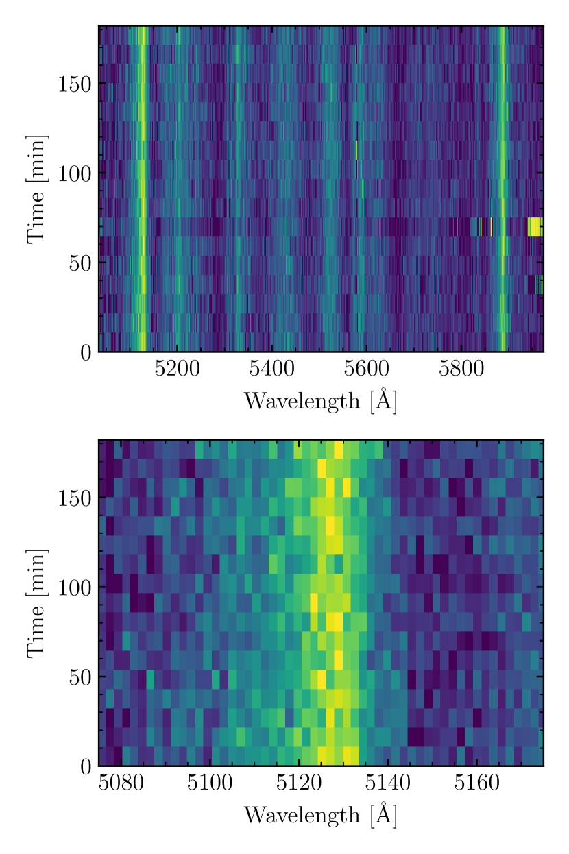
Figure 2: Trailed continuum-normalised spectra for our Gemini observations of SDSS J1143$+$6615. The top panel shows the entirety of chip-2, which contains both of the sharp features suggested to be from Mg and Na. The bottom panel shows a Zoom-in of the suggested Mg line, demonstrating an absence of spectral variability on a 3 hr timescale.

Given the lack of variability between our 17 spectra, we chose to co-add these into a single high S/N spectrum. We show this in the bottom of Figure 1 (dark grey). This is compared with the SDSS spectrum (light grey) which has been convolved to the same spectral resolution as our Gemini data. Almost all features appear unchanged, with perhaps only minor differences in the core strengths of the 5400 Å and 5500 Å features, and a slight change in wavelength of the feature at 4650 Å. This comparison demonstrates a lack of variability on a time scale of two years.

With the higher S/N spectrum, the proposed Na i and Mg i lines are seen to be blue shifted by 5.5 Å and 52 Å respectively. The asymmetric nature of the latter (discussed in Section 2.1), is also much clearer. For the proposed Na i line this could be plausibly explained as a $\simeq 300$km s^-1 blue shift (not including any gravitational redshift from the white dwarf) if SDSS J1143$+$6615 is a halo object. That being said, the much slower $18\pm 2$ km s^-1 tangential velocity from Gaia EDR3 (see Section 2.3) argues against this explanation. Furthermore, such an explanation is effectively ruled out by the proposed Mg i line, since its much larger wavelength shift would correspond to a velocity shift of about 3000 km s^-1. Therefore magnetism remains a more likely hypothesis for explaining the spectrum of SDSS J1143$+$6615. In addition to the lines observed from the SDSS spectrum, the Gemini spectrum also reveals the possible presence of the Ca i resonance line (Figure 1, purple), with a small blue shift of 1.6 Å.

2.3 Gaia

Despite its curious spectrum containing many anomalous features precluding obvious spectroscopic classification, the measured non-zero proper-motion by SDSS confirms that SDSS J1143$+$6615 is a galactic object. However, without knowing the absolute brightness of this star, SDSS J1143$+$6615 could not be claimed to be a white dwarf with certainty.

In April 2018, the second data release (DR2) from Gaia space mission made public approximately 1 billion parallaxes (Gaia Collaboration et al., 2018). This included SDSS J1143$+$6615 which had a measured parallax of $7.79\pm 0.68$ mas, confirming this stars location along the white dwarf cooling track within the Hertzsprung-Russel diagram (HR-diagram). In December 2020 a refined parallax of $7.24\pm 0.46$  mas was made available from Gaia EDR3 (early data release 3, Gaia Collaboration et al., 2021) corresponding to a distance of $138.8\pm 9.0$ pc. The EDR3 HR-diagram is shown in Figure 3. SDSS J1143$+$6615 is indicated by the red point, and is compared against a background of white dwarfs selected from Gentile Fusillo et al. (2021) with $\mbox{{PWD}}>0.75$ and $\mbox{{parallax\_over\_error}}>20$. From its location in the HR-diagram, it is clear that SDSS J1143$+$6615 is a cool white dwarf with a typical mass. Therefore Gentile Fusillo et al. (2021) found $\mbox{$T_{\mathrm{eff}}$}=5810\pm 460$ K and $\log g=8.17\pm 0.33$ fitting the Gaia photometry with pure hydrogen atmosphere models, and $\mbox{$T_{\mathrm{eff}}$}=5680\pm 470$ K and $\log g=8.08\pm 0.33$ for a pure helium atmosphere models. Interestingly, if Figure 3 is recreated using Gaia DR2 data, SDSS J1143$+$6615 appears to be offset from the white warf sequence towards higher masses, with Gentile Fusillo et al. (2019) finding $\mbox{$T_{\mathrm{eff}}$}=6990\pm 710$ K and $\log g=8.73\pm 0.29$ for hydrogen atmosphere models, and $\mbox{$T_{\mathrm{eff}}$}=6870\pm 750$ K and $\log g=8.67\pm 0.33$ for helium atmosphere models. That said, these parameter shifts amount to only $1.4\sigma$ changes at most and so are in statistical agreement.

Figure 3: Gaia EDR3 Hertzsprung-Russel diagram showing the location of SDSS J1143$+$6615 (red) compared with the white dwarf cooling sequence (grey histogram). The error bars represent $1\sigma$ uncertainties.

3 Atomic data calculations

To test our hypothesis that SDSS J1143$+$6615 is a highly magnetic DZ white dwarf, we required accurate wavelengths of (at the very least) the Na i and Mg i lines as a function of the magnetic field. For large magnetic field strengths, however, approaches that are based on a perturbative treatment of the magnetic field are no longer adequate and hence accurate finite-field quantum-chemical methods need to be employed. In these methods, the magnetic field is treated explicitly in the calculation of ground-state energies, excitation energies, and transition-dipole moments, thereby employing the electronic Hamiltonian for an $N$-electron system in a static magnetic field in the $z$-direction (the gauge-origin is here in the origin of the coordinate system)

$$\hat{H}=\hat{H}_{0}+\frac{1}{2}B\hat{L}_{z}+B\hat{S}_{z}+\frac{1}{8}B^{2}\sum_{i}^{N}(x_{i}^{2}+y_{i}^{2}),$$ (1)

where $B$ is the magnetic-field strength and $\hat{H}_{0}$ is the field-free atomistic (or molecular) Hamiltonian, consisting of the kinetic energy of the electrons, the nuclear-electronic potential and the electron-electron repulsion. $\hat{L}_{z}=\sum_{i}^{N}\hat{l}_{i,z}$ and $\hat{S}_{z}=\sum_{i}^{N}\hat{s}_{i,z}$ are the $z$-components of the angular momentum operator, and spin, respectively. The terms linear in the magnetic field are the orbital-Zeeman (responsible for the splitting of the orbitals) and spin-Zeeman terms (responsible for splitting according to spin parallel or antiparallel to the magnetic field), respectively. The quadratic term is referred to as diamagnetic contribution which always increases the energy of the system. As in the field-free case in quantum chemistry, FCI theory is not applicable for problems like ours due to its high computational cost. Instead, Coupled-Cluster (CC) theory (Shavitt & Bartlett, 2009) can be used, which has a more economical computational scaling. CC methods work with an exponential parametrization of the wave function $\Psi_{\mathrm{CC}}=\mathrm{e}^{\hat{T}}\Phi_{0}$, where $\hat{T}=\hat{T}_{1}+\hat{T}_{2}+\dots+\hat{T}_{N}$ is the so-called cluster operator generating excitations. $\hat{T}$ contains amplitudes (weighting coefficients in the wave functions) that are determined by solving the CC equations

$$\langle\Phi_{I}\mid\mathrm{e}^{-\hat{T}}\hat{H}\mathrm{e}^{\hat{T}}\mid\Phi_{0}\rangle=0.$$ (2)

The CC energy is then given as

$$E_{\mathrm{CC}}=\langle\Phi_{0}\mid\mathrm{e}^{-\hat{T}}\hat{H}\mathrm{e}^{\hat{T}}\mid\Phi_{0}\rangle.$$ (3)

Truncations in $\hat{T}$ as well as limiting the projection space define approximate CC schemes. For example, CC ‘singles doubles’ (CCSD) is defined with

$$\hat{T}^{\mathrm{CCSD}}=\hat{T}_{1}+\hat{T}_{2}$$

and projection on singly and doubly excited determinants. Analogously, in CC ‘singles doubles triples’ (CCSDT), $\hat{T}$ is truncated to

$$\hat{T}^{\mathrm{CCSDT}}=\hat{T}_{1}+\hat{T}_{2}+\hat{T}_{3}$$

and projection is additionally also performed on triply excited determinants. While CC is used to describe the ground-state wave function, Equation-of-Motion-CC (EOM-CC) (Shavitt & Bartlett, 2009) can also describe electronically excited states (EE). An operator $\hat{R}$, parametrized similarly as $\hat{T}$ acts on a CC wave function $\Psi_{\mathrm{exc}}=\hat{R}\Psi_{\mathrm{CC}}$. The corresponding amplitudes are determined via the solution of the eigenvalue problem in matrix form

$$\mathbf{\bar{H}r}=\Delta\mathbf{E}_{\mathrm{exc}}\mathbf{r}$$ (4)

in which an element of the matrix $\mathbf{\bar{H}}$ is given as

$$\bar{H}_{IJ}=\langle\Phi_{I}\mid\mathrm{e}^{-\hat{T}}(\hat{H}-E_{\mathrm{CC}})\mathrm{e}^{\hat{T}}\mid\Phi_{J}\rangle$$ (5)

and the vector $\mathbf{r}$ contains the amplitudes for the excitations. An overview of ff-CC and ff-EOM-CC methods can be found in Stopkowicz (2017). In this work, we have used various flavors of ff-CC theory (Stopkowicz et al., 2015; Kitsaras & Stopkowicz, 2022a) and ff-EOM CC theory, implemented within the QCUMBRE program package (Hampe & Stopkowicz, 2017), to determine excited states and hence transition wavelengths (Hampe & Stopkowicz, 2017; Hampe et al., 2020; Kitsaras & Stopkowicz, 2022a). The underlying calculation of the reference $|\Phi_{0}\rangle$ is performed with the CFOUR program package (Matthews et al., 2020). In the EOM-framework, we have employed the methods for electronic excitations (EE), spin flip (SF), adding electrons (EA, electron attachment) and removal of electrons (IP, ionization potential). Oscillator strengths are also treated at the expectation value ff-EOM-CC level (Hampe & Stopkowicz, 2019) which enables the prediction of field-dependent intensities. The transitions for which we have performed ff-calculations are displayed in Table 1.

Table 1: Level information for the transitions we have performed ff-calculations for. Wavelengths (air) correspond to field-free transitions, which in the case of multiplets corresponds to the average wavelength given in the NIST database (weighted by oscillator strength).

Ion	Wavelength [Å]	Lower state	Upper state
Na i	5892	${}^{2}S_{g}([\text{Ne}]3s)$	${}^{2}P_{u}([\text{Ne}]3p)$
Mg i	5178	${}^{3}P_{u}([\text{Ne}]3s3p)$	${}^{3}S_{g}([\text{Ne}]3s4s$)
Ca i	4227	${}^{1}S_{g}([\text{Ar}]4s^{2})$	${}^{1}P_{u}([\text{Ar}]4s4p)$
Ca i	6142	${}^{3}P_{u}([\text{Ar}]4s4p)$	${}^{3}S_{g}([\text{Ar}]4s5s)$
Ca ii	3945	${}^{2}S_{g}([\text{Ar}]4s)$	${}^{2}P_{u}([\text{Ar}]4p)$

The data for Na has partly already been available in Hampe et al. (2020). The latter work is also the basis for the computational protocol. We will here only mention the most important points and refer to Hampe et al. (2020) for further details. For all transitions, the calculations were performed for magnetic fields ranging between 0.00–0.04 B₀, with the atomic unit of the magnetic field, B₀ $\simeq 2350.518$ MG, using a 0.004 B₀ step and between 0.04–0.20 B₀ using a 0.02 B₀ step. In the protocol, a corrected excitation energy is computed according to

$$\Delta E_{\mathrm{exc}}^{\mathrm{corrected}}=\Delta E_{\mathrm{exc}}+\Delta E_{\mathrm{basis}}+\Delta E_{\mathrm{triples}},$$ (6)

where $\Delta E_{\mathrm{exc}}$ is the excitation energy computed using a large uncontracted augmented one-electron basis set. $\Delta E_{\mathrm{basis}}$ is a term correcting the one-electron basis-set error as described in Halkier et al. (1998) by extrapolating a basis-set limit $E^{\infty}$ based on uncontracted basis sets of the type aug-cc-pCVXZ (Kendall et al., 1992; Woon & Dunning, Jr., 1995), abbreviated as aCXZ, where X is the cardinal number. It is given as $\Delta E_{\mathrm{basis}}=\Delta E^{\infty}-\Delta E_{\mathrm{exc}}$ with

$$\Delta E^{\infty}=\frac{\Delta E_{\mathrm{exc}}^{\mathrm{aCXZ}}X^{3}-\Delta E_{\mathrm{exc}}^{\mathrm{aCYZ}}Y^{3}}{X^{3}-Y^{3}}.$$ (7)

The $\Delta E_{\mathrm{triples}}=E_{\mathrm{triples}}^{\mathrm{aCXZ}}-E_{\mathrm{exc}}^{\mathrm{aCXZ}}$ correction accounts for the error which stems from truncating the CC expansion and involves computations at the ff-EOM-CCSDT (Hampe et al., 2020), ff-EOM-CC3 (Kitsaras & Stopkowicz, 2022a) or ff-EOM-CCSD(T)(a)* (Matthews & Stanton, 2016; Kitsaras & Stopkowicz, 2022b) levels of theory for $E_{\mathrm{triples}}^{\mathrm{aCXZ}}$ using a smaller basis set. The accuracy and cost is typically CCSDT ($O(M^{8})$)> CC3 ($O(M^{7})$)> CCSD(T)(a)* ($O(M^{7})$) where $M$ is the number of basis functions. In the latter two, triple-excitations are treated in a perturbative manner. CC3 is iterative while CCSD(T)(a)* is not. The latter is a very good and relatively cheap option when the target-states are characterised mostly by single-excitation character. The dimensionless oscillator strengths $f_{IJ}$ were calculated according to

$$f_{IJ}=\frac{2}{3}(\Delta E_{IJ})|\mu_{IJ}|^{2},$$ (8)

where $\Delta E_{IJ}$ is the excitation energy from states $I$ to $J$ and $\mu_{IJ}$ is the corresponding transition-dipole moment, and where both $\Delta E_{IJ}$ and $\mu_{IJ}$ are in atomic units. After converting the (field-dependent) excitation energies to transition wavelengths, the resulting $B-\lambda$ curves were shifted to start at the zero-field values taken from the NIST database (Kramida et al., 2022) thereby correcting for remaining errors of our predictions at zero field. The spin-orbit contributions have been averaged out as their contribution is expected to be small for stronger fields. By the shift made to the NIST data, field-free scalar-relativistic effects are implicitly accounted for. For the time being, we are neglecting relativistic effects and in particular their dependence on the magnetic field in our calculations as the effects are expected to be small for strong magnetic fields. This approximation is better for the lighter elements Na and Mg than for the heavier Ca. The specific details on the calculations are collected in Table 2.

Table 2: Detailed information on ff-EOM calculations for the respective transitions. If not specified otherwise, $\Delta E_{IJ}$, see Eq. (8), has been calculated at the same level as $\mu_{IJ}$

Transition	Basis functions	$\Delta E_{\mathrm{exc}}$	$\Delta E_{\mathrm{basis}}$	$\Delta E_{\mathrm{triples}}$	$\mu_{IJ}$
Na i	Cartesian	EE-CCSD/aCQZ	EE-CCSD/aCXZ, X=T, Q	CCSDT/aCTZ	EE-CCSD/aCQZ
Mg i	Spherical	EE-CCSD/aC5Z	EE-CCSD/aCXZ, X=Q, 5	CC3/aCQZ	EE-CCSD/aC5Z
Ca i 4227	Spherical	EE-CCSD/aC5Z	EE-CCSD/aCXZ, X=Q, 5	EE-CC3/aCQZ	EE-CCSD/aCQZ(a)
Ca i 6142	Spherical	SF-CCSD(T)(a)*/aC5Z	SF-CCSD(T)(a)*/aCXZ, X=Q, 5	No further triples correction	SF-CCSD/aC5Z(b)
Ca ii	Spherical	EA-CCSD/aC5Z	EA-CCSD/aCXZ, X=Q, 5	EE-CCSD(T)(a)*/aCQZ	EA-CCSD/aC5Z(c)

Notes: ($a$) $E_{IJ}$ calculated using EE-CC3, ($b$) Reference for SF calculations: ${}^{1}S_{g}$ ([Ar] $4s^{2}$), ($c$) Reference for EA calculations: ${}^{1}S_{g}$([Ar])

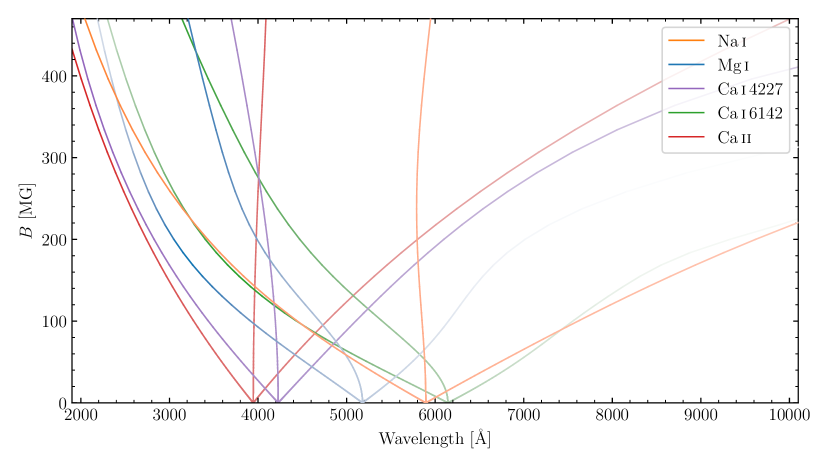
Figure 4: Calculated transition wavelengths as a function of field strength. For each Zeeman triplet, the line opacities are scaled to the oscillator strengths.

The predicted transition wavelengths and oscillator strengths can be found in Tables 3–7. Additionally, the obtained $B-\lambda$ curves are shown in Fig. 4. The intensity of the transitions, i.e. oscillator strengths, are indicated via the opacities of the curves. As all of the investigated transitions are of $ns\rightarrow np$ or $np\rightarrow(n+1)s$ type, where $n$ is the main quantum number of the orbital (without field), there is in all cases a splitting into three components, i.e., the central $\pi$ (transition from/into a $p_{0}$ orbital) as well as the two $\sigma$ (transition from/into $p_{+1}$ and $p_{-1}$) components. As can be seen here, the splitting is only linear for fields below about 5–10 MG while for higher field strengths, the form of the $B-\lambda$ curves becomes much more complicated. The distortion from a simple Zeeman behaviour is transition dependent: For the $np\rightarrow(n+1)s$ transitions (Mg and Ca i 6142), the influence of the magnetic field on the central $\pi$ component is much more pronounced than for the $ns\rightarrow np$ transitions (Na, Ca ii, Ca i 4227). The principal reason for this behaviour is that in the former case the transitions are between orbitals of different main quantum numbers. The orbitals hence experience a different amount of polarisation through the magnetic field, i.e. those of higher main quantum number are polarised more strongly due to their more diffuse nature. Effectively this means that the $s$ and $p_{0}$ orbitals and the respective electronic states, don’t evolve in a parallel manner with increasing magnetic field. Hence, in contrast to the simple perturbative picture, the central $\pi$ component is no longer constant with increasing magnetic field strength. In addition, the transitions with decreasing energy difference in the magnetic field, i.e., $ns\rightarrow np_{-1}$ and $np_{+1}\rightarrow(n+1)s$ become less relevant for observations, as they decrease in intensity (see Equation (8)). In addition, small changes in the magnetic field lead to large changes in the transition wavelength and hence such transitions will be blurred out in the spectra for strong fields. A more detailed discussion on the form of the energy levels and the resulting for of the $B-\lambda$ curve of the Mg transition can be found in Kitsaras & Stopkowicz (2022a). As noted in Hampe et al. (2020), high-accuracy predictions are required as even the prediction for the transition least affected by the magnetic field, i.e., the central $\pi$ component of Na can vary by up to 100 Å depending on the level of theory and basis set used.

4 Line identification

With the wavelengths and oscillator strengths calculated in Section 3, we were able to compare these with the spectrum of SDSS J1143$+$6615. With no immediate indication of which spectral features could correspond to the $\sigma$-components of the calculated transitions, we began by restricting ourselves to the $\pi$-components only. In Section 2 we identified possible $\pi$-components of Na i, Mg i, and Ca i in the SDSS and GMOS spectra, based on the sharpness of the lines, rough proximity in wavelengths to the field-free values, and characteristic asymmetry in the case of Mg.

We compare these lines to our calculated wavelengths as a function of field strength in the top panels of Figure 5. From the bottom-right panel, it is clear that the Na line shift could be explained by either a relatively small field of $\simeq 30$ MG or much larger field of $\simeq 410$ MG, owing to a turnaround in wavelength at $\simeq 240$ MG. This degeneracy is entirely resolved by the large shift of the Mg line which has only one wavelength solution and is also consistent with a field of $\simeq 30$ MG. Thus, to our surprise, the peculiar spectrum of SDSS J1143$+$6615 (Figure 1) can not result from a field in the regime of 100s of MG, but is best explained by a field strength an order of magnitude lower, though notably still a factor three higher than all previously identified DZH white dwarfs (Hollands et al., 2015, 2017; Dufour et al., 2015).

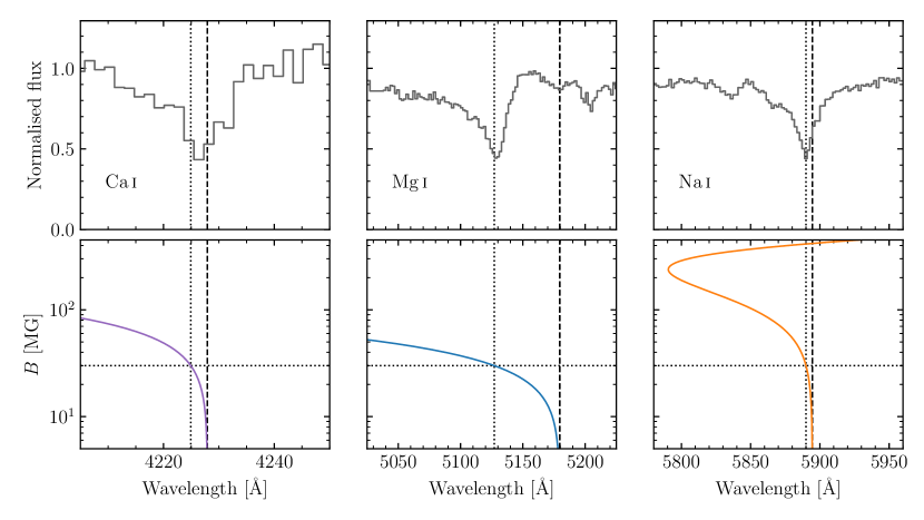
Figure 5: Top row: Spectral regions covering the suspected $\pi$-components of Ca i, Mg i, and Na i. Bottom row: Predicted wavelengths for the corresponding $\pi$-components as a function of field strength. In all panels the black dashed lines indicate the field-free vacuum wavelengths for each line, whereas the dotted lines indicate the wavelengths expected for a 30 MG field.

For Ca i the match in wavelength is quite poor, though thus far we have neglected wavelength shifts that may arise from radial motion and gravitational redshift, the latter of which could be on the order of 100 km s^-1 if SDSS J1143$+$6615 is particularly massive, which is typically the case for magnetic white dwarfs (Liebert, 1988; Kawka et al., 2020; Ferrario et al., 2020). Additionally, the absent treatment of relativistic effects may here play a role in the quality of the prediction. It is also clear that at 30 MG, the predicted wavelength for Mg is a similar amount bluer than the line centre (though with greater relative accuracy). To account for this we fitted the field strength and radial velocity simultaneously. We measured the line centres for all three $\pi$-components by simply fitting parabolas to the central few pixels (five for Ca and seven for Mg and Na), constraining them with uncertainties of 0.1–0.3 Å. Performing a least squares fit to the three line centres, we found a magnetic field strength of $29.92\pm 0.05$ MG and a redshift of $74\pm 8$ km s^-1. With these best fitting values the residuals are $-0.7$ Å, $0.0$ Å, and $1.8$ Å for the Ca, Mg, and Na lines, respectively. This was a clear improvement for Ca i and Mg i, though provides a somewhat worse result for the Na i line.

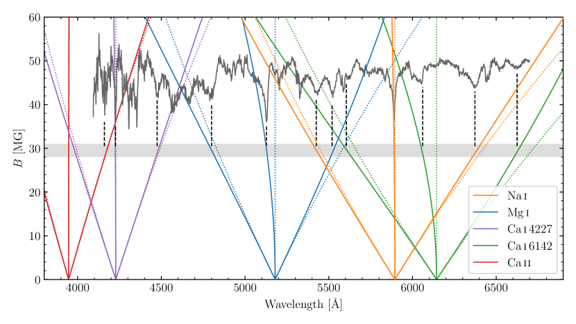
Figure 6: Line identification diagram for SDSS J1143$+$6615. The Zeeman triplets from our finite-field coupled-cluster calculations are shown by the solid curves, with the naïve wavelengths from the linear Zeeman effect indicated by the dotted lines. These are plotted over the spectrum of SDSS J1143$+$6615 (grey), where black dashed lines match Zeeman components to features in the spectrum for a field strength of approximately 30 MG (light grey horizontal band).

With the field strength established from the $\pi$-components, we could then determine the expected wavelengths of the $\sigma$-components. We make this comparison in Figure 6. We first investigated the components of Na and Mg, with their $\sigma$-components identified with relative ease. In particular the large broad feature at $\simeq 6350$ Å is established as the $\sigma^{+}$ component of Na, which does not appear blended with any of the other nearby features. Near 5500 Å both the Na $\sigma^{-}$ and Mg $\sigma^{+}$ components are observed, though notably the order of their wavelengths has swapped due to the components crossing at a field strength of $\simeq 25$ MG. The Mg $\sigma^{-}$ component is inferred to be the broad, asymmetric feature at $\simeq 4800$ Å. The asymmetry appears more extreme than for the $\pi$-component, which itself is more asymmetric than the $\sigma^{+}$ component. This may imply that the degree of neutral broadening affects each component differently, which perhaps is not surprising given that both the perturbations from neutral helium atoms and the magnetic field both alter the energy levels of Mg.

Having identified all components from Na i and Mg i, we proceeded with classifying transitions from Ca. For the Ca i resonance line, we had already identified the $\pi$-component (rest wavelength at 4227 Å; see Figure 5, left). As our Gemini GMOS spectrum does not go bluer than about 4090 Å, the $\sigma^{-}$-component is not covered, and so we were only able to search for the $\sigma^{+}$ component which, at 30 MG, has an expected wavelength of 4475 Å. Indeed, a spectral feature was found at this wavelength which we attribute to the $\sigma^{+}$ component (Figure 6).

The final Ca transitions are less certain, though we still make some attempt at their classification. For the Ca ii Zeeman triplet (H+K resonance doublet in the absence of an external magnetic field), only the $\sigma^{+}$ component is expected to be covered by our GMOS spectrum at a field strength of 30 MG. While we detect a feature at the expected wavelength of 4160 Å (Figure 6), the signal-to-noise ratio is somewhat poor at this end of the spectrum, making this assignment less secure. However, it is worth noting that for a $T_{\mathrm{eff}}$ between 5000 K and 7000 K, both Ca i and Ca ii resonance lines are typically observed together in non-magnetic DZs (Hollands et al., 2017).

Finally we consider the Ca i $4p\rightarrow 5s$ transition, which in the absence of an external magnetic field appears as a triplet (due to the spin-orbit interaction) centred on 6142 Å. In the presence of a strong magnetic field, this transition appears as a Zeeman triplet exhibiting the strongest quadratic shift of all the transitions calculated in Section 3. Nevertheless, weak transitions are observed at all of the expected wavelengths. Whether this assignment is correct is debatable: the identified central component at around 6060 Å shows some asymmetry, as is observed in the field-free case (see SDSS J0916$+$2540 in Figure 10 of Hollands et al., 2018a). On the other hand, the 6142 Å triplet is typically much weaker than the Ca i 4227 Å resonance line, and is only usually visible for extremely large calcium abundances. Yet, in the case of SDSS J1143$+$6615, the established components of the 4227 Å Ca i Zeeman triplet are not particularly strong, suggesting that the 6142 Å components would likely be too weak to be visible. Given the sheer number of unknown features in the spectrum of SDSS J1143$+$6615, it is probable that our assignments to the 6142 Å triplet in Figure 6 might also originate from some other source.

Many anomalous features in the spectrum of SDSS J1143$+$6615  remain unclassified. In particular two strong and broad features are observed at wavelengths of $\simeq 4570$ Å and $\simeq 4660$ Å, between the $\sigma^{+}$-component of the Ca i resonance line, and the $\sigma^{-}$-component of Mg i. The strength of these features suggest they originate from another element commonly observed in DZ spectra. With the strongest Na, Mg and Ca lines already accounted for, the most likely candidate is therefore Fe. In the field-free case, a large number of Fe i lines can be found between 4000–4500 Å (see Hollands et al., 2018a, Figure 7). Among the strongest transitions in this range are the ${}^{3}F\rightarrow\ ^{5}G$ and ${}^{3}F\rightarrow\ ^{3}G$ multiplets, which share the same lower level. We therefore suggest that the unidentified features at $\simeq 4570$ Å and $\simeq 4660$ Å arise from these iron transitions. Additional unidentified features include broad absorption around $4300$ Å (between the $\pi$- and $\sigma^{+}$-components of Ca i), sharp features at $\simeq 5200/5330/5580$ Å, and several other features at $\simeq 6030/6450/6530/6620$ Å (some of which we were unable to conclusively assign to the Ca i $6142$ Å multiplet). We note that the feature near 5200 Å is close to the field-free wavelength of the Cr i $4s\rightarrow 4p$ triplet (5208 Å, vacuum), and so that feature could plausibly correspond to the $\pi$-component of the Cr i transition. Firmly establishing the origin of these remaining features necessarily will require additional finite-field coupled-cluster calculations in the future, with the above Fe and Cr transitions as the highest priority. For these systems, treatment of field-dependent relativistic effects and a robust treatment of multi-reference character in the electronic structure will be important.

5 Magnetic field modelling

With several of the spectral features of SDSS J1143$+$6615 identified, we finally sought to model the magnetic field distribution across its surface. For a purely dipolar magnetic field, the field strength spans a factor of two between the equator and poles. This results in broadened spectral lines, particularly the $\sigma$-components due to their stronger wavelength dependence of the field strength. It is clear from the width of the Na i $\sigma^{+}$ component that the range of magnetic field strengths on the visible hemisphere of SDSS J1143$+$6615 spans a much narrower field range, with Figure 6 suggesting about 24–31 MG. Thus it is necessary to invoke a field structure more complex than a centred dipole.

5.1 The offset dipole model

We chose to use the offset-dipole model, which has been commonly used in the analysis of magnetic white dwarf field structures (Achilleos & Wickramasinghe, 1989). This model is similar to a centred-dipole, but allows for the origin of the field to be shifted within the white dwarf. In principle this shift can be applied in three dimensions, but typically it is only applied along the magnetic field axis by a fractional amount of the white dwarf radius, $a_{z}$. The offset-dipole model has been successfully applied to many different white dwarfs (Achilleos et al., 1992; Putney & Jordan, 1995; Külebi et al., 2009; Hollands et al., 2015) leading to much improved fits with only a single additional free-parameter, which is advantageous compared to a more general multi-pole expansion.

For a centred-dipole with the magnetic field aligned with the $z$-axis, the value of the magnetic field at any point on (and external to) the stellar surface in Cartesian coordinates ($x/y/z$) is given by,

$$\begin{bmatrix}B_{x}\\ B_{y}\\ B_{z}\end{bmatrix}=\frac{B_{d}}{2r^{5}}\begin{bmatrix}3xz\\ 3yz\\ 3z^{2}-r^{2}\end{bmatrix},$$ (9)

where $B_{x/y/z}$ are the Cartesian components of the magnetic field, $B_{d}$ is the polar field strength, and $r^{2}=x^{2}+y^{2}+z^{2}$. The offset-dipole model simply requires making the translation $z\mapsto z-a_{z}$, in Equation (9) and in the definition of $r^{2}$. To complete the offset-dipole model we also allow rotation between the magnetic field axis and the observer. We implement this by considering coordinate systems for both the magnetic field and the viewing direction of the observer, with a rotation matrix used to convert between them.

Using the above model of the white dwarf magnetic field structure, we construct a toy model spectrum by randomly sampling 10,000 points uniformly across the stellar disc (i.e. sampled uniformly within the unit circle). For each point on the stellar disc, $i$, we used Equation (9) to calculate the magnetic field vector (accounting for the chosen inclination). Then for each transition, $j$, we compute a Zeeman-triplet of three Lorentzian profiles, using our atomic data from Section 3 to determine their wavelengths and oscillator strengths. Furthermore, the $\pi$-component is scaled by a factor $\sin^{2}\psi/2$, and the $\sigma$-components by a factor $(1+\cos^{2}\psi)/4$, which accounts for linear and circular polarisation effects respectively (Putney & Jordan, 1995), and where $\psi$ is the angle between the field line and the observer’s line of sight. These three Lorentzian components are then summed to form an opacity function

$$\kappa_{ij}(\lambda;B_{i},\psi_{i})=\sum_{\Delta m_{l}=-1}^{+1}L_{j}(\lambda;B_{i},\psi_{i},\Delta m_{l}),$$ (10)

where $L_{j}$ are the Lorentzian profiles per transition. Finally, the normalised flux for all transitions at point $i$ is given by

$$F_{i}(\lambda;B_{i},\psi_{i})=\exp\left\{-\sum_{j}A_{j}\kappa_{ij}(\lambda;B_{i},\psi_{i})\right\},$$ (11)

where $A_{j}$ is a pseudo-abundance which we use to arbitrarily scale the strength of each Zeeman-triplet. Finally, we compute the integrated flux over the stellar disc as a weighted sum based on the centre-to-limb intensity of the stellar disc

$$F(\lambda)=\frac{\sum_{i}F_{i}(\lambda;B_{i},\psi_{i})I(\mu_{i})}{\sum_{i}I(\mu_{i})},$$ (12)

where $I(\mu_{i})$ is the intensity across the stellar disc, and where $\mu_{i}$ is equivalent to the $z$ coordinate of the $i$-th point on the stellar disc in the observers frame of reference. We use the logarithmic limb-darkening law for a 6000 K, $\log g=8$ white dwarf from Gianninas et al. (2013).

5.2 Application to SDSS J1143$+$6615

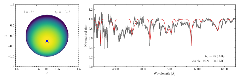
Figure 7: Left: Visualisation of the field structure of SDSS J1143$+$6615 modeled with an offset-dipole. Right: The simulated absorption spectrum of SDSS J1143$+$6615 (red) using data from our finite-field coupled cluster calculations.

We applied the offset dipole model to SDSS J1143$+$6615 initially focusing on the Na triplet. From analysing the $\pi$-components of Mg and Na in Section 4, we established a surface averaged field of $\simeq 30$ MG, and hence located the features corresponding to the $\sigma$-components. Due to the asymmetry of the Mg components we decided to begin our focus on the Na triplet. However, the $\sigma^{-}$ component of Na and the $\sigma^{+}$ component of Mg are somewhat overlapping ($\simeq 5500$ Å), and so we chose to restrict ourselves to the $\pi$ and $\sigma^{+}$ components of Na ($\simeq 6400$ Å). Overall we therefore had five parameters to adjust: the polar field strength $B_{d}$, the dipole-inclination, and the dipole-offset $a_{z}$, which controlled the field distribution; plus the Lorentzian line strength ($A_{j}$ in Section 5.1) and width which are most easily inferred by the relatively static $\pi$-component.

As described at the start of Section 5, the width of the $\sigma^{+}$ component of Na implies a field strength distribution narrower than the factor of two for a centred dipole. In the offset-dipole model a narrower distribution can be achieved for negative values of $a_{z}$, combined with a low inclination (i.e. viewed close to pole-on). This implies a wider distribution of field strengths on the opposite hemisphere of the star. Because $B_{d}$ in Equation (9) no longer corresponds to the field at the poles, for finite $a_{z}$, both parameters must be adjusted simultaneously to maintain a polar field strength of 30 MG on the visible hemisphere. Manipulating Equation 9, and making the substitution $z\mapsto z-a_{z}$, it can be shown that

$$B_{d}=(1-a_{z})^{3}B_{z=1},$$ (13)

where $B_{z=1}$ is the near-side pole strength of 30 MG. Adjusting these parameters by hand, we found good agreement with the shape of the Na $\sigma^{+}$-component could be achieved with $a_{z}=-0.15$ (implying $B_{d}=45.6$ MG from Equation (13)) and a dipole-inclination of $15$ degrees (Figure 7). This also yields a reasonable agreement with the $\sigma^{-}$-component (at wavelengths where it is not blended with the $\sigma^{+}$-component from Mg). We then included all other transitions from Section 3 into the model adjusting only the strengths and widths of the Lorentzian profiles. A further refinement is required for the Mg i and Ca i 6142 Å triplets as these are $np\rightarrow(n+1)s$ transitions (the others are all $ns\rightarrow np$), and so we scale the component strengths by Boltzmann factors reflecting the different occupation levels of the lower states.

Unsurprisingly, the Lorentzian profiles used provide a poor fit for the asymmetric $\pi$- and $\sigma^{-}$-components of Mg i, though reasonable agreement is found for the $\sigma^{+}$-component. As discussed previously, this may indicate that the degree of neutral broadening is field-dependent, and affects the bluer components more strongly. For the Ca i 4227 Å resonance line, when the width and strength parameters are adjusted to match the $\pi$-component, the strength and shape of the $\sigma^{+}$-component ($\simeq 4090$ Å) also agree well with the observations. This demonstrates that the values of $B_{d}$, $a_{z}$, and the inclination found from the Na lines are also appropriate for this transition. For the Ca ii triplet, the width of the $\sigma^{+}$ component is also seen to be in agreement with the data, though the signal-to-noise ratio in this part of the spectrum is too poor to compare the shape of the line with the data. Finally for the Ca i 6142 Å Zeeman-triplet, only the shape of the $\sigma^{+}$-component in is reasonable agreement with the data, furthering the argument from Section 4 that these transitions may originate from another source.

6 Discussion

6.1 DZs with much stronger fields

In Section 5, we constructed a toy-model for generating simplified magnetic DZ spectra, including atomic data from Section 3. While it turned out that SDSS J1143$+$6615 has only a 30 MG field, in principle our model allows us to generate synthetic spectra for much larger fields, with 470 MG covering all the transitions we calculated in Section 3. Since ongoing/upcoming spectroscopic surveys such as WEAVE, DESI, SDSS V, and 4MOST, are expected to yield hundreds of thousands of white dwarf spectra in the next decade, we investigate which transitions ought to be focused on for identifying even higher field DZ stars in the future.

In Figure 8, we show models with average surface fields spanning 25–400 MG against the same curves from Figure 4. For all five models, we used the same inclination and dipole offset as found for SDSS J1143$+$6615, i.e. 15 degrees and $-0.15$ respectively. Note that the $B_{s}$ values are the surface averaged field strengths whereas the dipole field strength, $B_{d}$, is approximately 52 percent larger (see Equation 13).

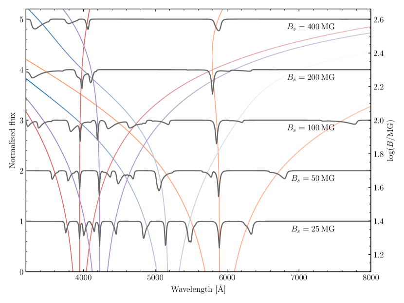
Figure 8: Simulated magnetic DZ spectra for five different surface averaged field strengths ($B_{s}$), with each spectrum offset from one another by 1 in normalised flux. The inclination and dipole offset parameters are fixed to the values found for SDSS J1143$+$6615 (i.e. 15 degrees and $-0.15$, respectively). The background Zeeman triplets have the same meaning as in Figure 4, with the field strength scale given on the right-hand axis.

The bottom model has a field $B_{s}=25$ MG, similar in strength to that found for SDSS J1143$+$6615, and thus shows a similar spectrum. Despite the relatively uniform field for an inclination of 15 degrees and $a_{z}=-0.15$, as the field increases, the $\sigma$-components still become washed out, and for most of the transitions are almost invisible at fields of around 100 MG and above. For Mg i the $\sigma^{+}$ component still remains visible above 100 MG due to its increase in oscillator strength.

On the other hand, most of the $\pi$-components remain relatively steady in wavelength. For the Na $\pi$-component, as already noted in Hampe et al. (2020), the wavelength changes very little below $100$ MG, leaving this line similarly sharp as for a 25 MG field. The Na line reaches a maximum in blue-shift at 240 MG (100 Å bluer than the field free wavelength), before rapidly turning around and moving to redder wavelengths. Therefore for $B_{s}=400$ MG, the line becomes much broader, but remains clearly visible. Therefore this transition ought to be used as a primary marker for identifying cool magnetic DZ white dwarfs with $>100$ MG fields.

Similarly the Ca i $\pi$-component remains relatively stationary up to $100$ MG, but becomes more washed out for larger fields due to the quadratic Zeeman effect, and becoming broadened to a width of 100 Å at $400$ MG. Therefore this line is likely to be less reliable than the Na $\pi$-component for identifying the highest field DZs, but will still remain reliable up to 200 MG.

The Ca ii $\pi$-component is also near stationary, and should still be recognisable even at 400 MG, making this a more obvious choice for identifying warmer high field DZs where the Na i and Ca i lines may be too weak to identify. Note that at 300 MG, the Ca i and Ca ii $\pi$-components overlap producing a blended spectral feature.

Finally, the Mg i $\pi$-component experiences a much larger quadratic shift than the other transitions considered here. Therefore at 400 MG, the line appears broad and asymmetric though is notably still visible, in part due to the increased oscillator strength for this component, which is close to four times larger than in the field-free case, thereby also showcasing the importance of considering field-dependent intensities. Note that this toy-model does not consider the intrinsic asymmetry caused by neutral broadening, which itself could be a function of field strength.

A final consideration is that we have not yet identified all the features in the spectrum of SDSS J1143$+$6615. Therefore at very high field strengths of 100s of MG, these unclassified features will also appear shifted into other parts of the spectrum further complicating the identification of the transitions discussed above. Furthermore, other strong lines outside the optical such as the Mg i and Mg ii resonance lines (field free wavelengths at 2853 Å and 2799 Å, respectively), may find some of their Zeeman split components shifted into the optical providing other atomic features requiring identification.

6.2 Use in model atmospheres

Ideally the atomic data we have presented in Section 3 can be utilised in white dwarf model atmospheres for more detailed analyses of magnetic DZ stars. As we have shown in this work, however, this is not necessary for a basic assessment. For simply determining the surface-average field strength, $B_{s}$, and which ions are present in the atmosphere, it is sufficient to simply compare our atomic data with the spectrum in question, as was demonstrated in Section 4 for SDSS J1143$+$6615. Furthermore, determining the field structure of a white dwarf can be achieved with a simple model such as the toy-model we demonstrated in Section 5. Importantly our toy-model is computationally efficient, taking only a few seconds to produce Figure 7.

Of course, much can still be learned from incorporating our atomic data into model atmospheres. In our toy-model from Section 5, the strength and widths of the Lorentzian profiles we used have no physical basis, and are simply adjusted to give acceptable agreement with the data. In a model atmosphere, the strengths and widths of the features seen in the spectrum of SDSS J1143$+$6615 can be investigated by adjusting the abundances and $T_{\mathrm{eff}}$ (and to some extent the surface gravity) of the model, allowing these atmospheric properties to be measured in a physically meaningful way.

The main challenge of such an approach is the computation time required. In the field-free case, the final model spectrum is integrated over the stellar disc from spectra calculated at different angles between the surface-normal and the observer. For finite-fields, however, the synthetic spectra must also be calculated over a grid of field strengths and angles between the field and observer. In particular, the field strength axis of the grid must be computed at sufficiently fine steps so that artefacts from undersampling are not present when integrating over the stellar disc. Therefore, depending on the range of field strengths required, computation may take hundreds to thousands of times longer than in the field-free case. If the $T_{\mathrm{eff}}$, $\log g$, or abundances require refinement when comparing against a particular spectrum, the grid must then be recomputed with updated atmospheric parameters, leading to an even larger amount of computation time.

For that reason we have refrained from including our atomic data within model atmospheres at the present time, and also because it exceeds the scope of our primary goals of classifying the spectral features of SDSS J1143$+$6615 and measuring its field strength. However, future work should perform a detailed atmospheric analysis of SDSS J1143$+$6615 utilising the atomic data presented here to measure its $T_{\mathrm{eff}}$, $\log g$, and abundances.

7 Conclusions

We have identified SDSS J1143$+$6615 as DZ white dwarf with strong magnetic field resulting in its unique spectrum. Using finite-field, coupled-cluster calculations we were able to identify lines from Na i, Mg i, and Ca i–ii that were split and shifted by the linear and quadratic Zeeman effects. This also allowed us to establish a field strength of $\simeq 30$ MG, demonstrating that DZ spectra are challenging to interpret at only a few 10 MG, due to multiple overlapping transitions from a variety of chemical elements, which is not the case for magnetic DAs or DBs at the same field strength. Using the offset-dipole model, we were able to obtain an adequate fit to the spectral features of Na with an almost pole-on observation angle, and the dipole offset away from the observer.

Despite our success in elucidating some of the peculiar features in the spectrum of SDSS J1143$+$6615, many transitions still lack classification at the present time. Giving consideration to the elements and lines most commonly encountered in non-magnetic cool DZ stars, future atomic data calculations should concentrate on Fe and Cr lines, as well as additional transitions of Ca. Because SDSS J1143$+$6615 is currently the only available test for these calculations, and only samples the relatively low-field end, searching for additional high-field DZs within ongoing and future spectroscopic surveys (such as SDSS V, WEAVE, and DESI) is imperative to test the accuracy of our atomic data further at field strengths of many 100 MG.

Data Availability

All observations of SDSS J1143$+$6615 are either public (SDSS, Gaia) or no longer proprietary (Gemini). The Gemini data can be be obtained from the Gemini Observatory Archive, using program ID GN-2015B-FT-29. Atomic data calculations presented in this work are available in the appendix tables.

Appendix A Atomic data tables

Table 3: Atomic data for the Na i Zeeman triplet under an applied magnetic field. The magnetic field strength $B$, is given in both atomic units and in MG. Wavelengths are given in vacuum form. Oscillator strengths are calculated according to Equation (8).

		Wavelength [Å]			Oscillator strength
$B$ [B0]	$B$ [MG]	$\sigma^{-}$	$\pi$	$\sigma^{+}$	$\sigma^{-}$	$\pi$	$\sigma^{+}$
0.000	0.0	5894.571	5894.571	5894.571	0.324	0.324	0.324
0.004	9.4	5742.745	5894.121	6048.521	0.332	0.324	0.316
0.008	18.8	5593.316	5892.750	6204.298	0.341	0.325	0.307
0.012	28.2	5446.622	5890.503	6361.706	0.349	0.325	0.299
0.016	37.6	5302.977	5887.427	6520.591	0.358	0.325	0.291
0.020	47.0	5162.697	5883.594	6680.899	0.367	0.325	0.284
0.024	56.4	5026.005	5879.071	6842.550	0.375	0.325	0.275
0.028	65.8	4893.157	5873.968	7005.660	0.383	0.325	0.268
0.032	75.2	4764.303	5868.374	7170.305	0.391	0.326	0.260
0.036	84.6	4639.560	5862.401	7336.642	0.400	0.326	0.253
0.040	94.0	4519.034	5856.224	7504.982	0.408	0.326	0.246
0.060	141.0	3978.205	5824.551	8382.905	0.444	0.327	0.211
0.080	188.0	3532.705	5800.229	9351.385	0.475	0.328	0.180
0.100	235.1	3166.158	5790.578	10456.342	0.501	0.328	0.152
0.120	282.1	2862.247	5797.779	11753.431	0.523	0.327	0.127
0.140	329.1	2607.352	5820.542	13310.699	0.541	0.325	0.106
0.160	376.1	2390.966	5855.747	15218.789	0.557	0.324	0.087
0.180	423.1	2205.210	5899.663	17609.247	0.570	0.322	0.071
0.200	470.1	2044.197	5948.392	20689.341	0.581	0.320	0.057
0.220	517.1	1903.490	5998.674	24813.862	0.590	0.319	0.045
0.240	564.1	1779.628	6048.357	30631.655	0.597	0.318	0.035
0.260	611.1	1669.853	6095.463	39457.890	0.603	0.318	0.026
0.280	658.1	1571.985	6139.070	54464.836	0.608	0.319	0.018
0.300	705.2	1484.230	6179.092	85612.964	0.611	0.319	0.011
0.320	752.2	1405.100	6215.124	188444.928	0.613	0.320	0.005
0.340	799.2	1333.383	6247.316	1320875.762	0.614	0.322	0.001
0.360	846.2	1268.067	6275.954	153882.824	0.615	0.324	0.005
0.380	893.2	1208.306	6301.160	84066.792	0.614	0.325	0.009
0.400	940.2	1153.390	6322.883	59099.755	0.613	0.327	0.012
0.420	987.2	1102.746	6341.015	46374.747	0.611	0.329	0.015
0.440	1034.2	1055.874	6355.731	38758.544	0.609	0.331	0.017
0.460	1081.2	1010.555	6366.008	35866.670	0.608	0.333	0.017
0.480	1128.2	971.855	6371.932	30295.527	0.604	0.335	0.019
0.500	1175.3	934.065	6372.374	27799.155	0.601	0.337	0.020

Table 4: Atomic data for the Mg i Zeeman triplet under an applied magnetic field. Columns have the same meaning as in Table 3.

		Wavelength [Å]			Oscillator strength
$B$ [B0]	$B$ [MG]	$\sigma^{-}$	$\pi$	$\sigma^{+}$	$\sigma^{-}$	$\pi$	$\sigma^{+}$
0.000	0.0	5179.597	5179.597	5179.597	0.138	0.135	0.137
0.004	9.4	5061.068	5174.347	5294.864	0.157	0.136	0.120
0.008	18.8	4940.130	5158.717	5406.135	0.177	0.137	0.105
0.012	28.2	4817.641	5133.057	5512.746	0.199	0.139	0.092
0.016	37.6	4694.469	5097.935	5614.167	0.224	0.142	0.080
0.020	47.0	4571.460	5054.112	5710.030	0.250	0.146	0.070
0.024	56.4	4449.419	5002.504	5800.152	0.279	0.150	0.060
0.028	65.8	4329.099	4944.155	5884.567	0.309	0.156	0.052
0.032	75.2	4211.181	4880.187	5963.528	0.341	0.163	0.045
0.036	84.6	4096.271	4811.771	6037.528	0.373	0.171	0.038
0.040	94.0	3984.896	4740.081	6107.286	0.407	0.181	0.033
0.060	141.0	3493.822	4370.457	6432.470	0.556	0.249	0.013
0.080	188.0	3125.114	4054.666	6862.945	0.576	0.345	0.004
0.100	235.1	2863.579	3828.322	7609.333	0.451	0.430	0.001
0.120	282.1	2672.345	3666.824	8859.285	0.307	0.479	0.000
0.140	329.1	2521.311	3537.491	10899.854	0.201	0.504	0.000
0.160	376.1	2394.409	3422.271	14450.113	0.127	0.518	0.000
0.180	423.1	2283.908	3313.842	21816.811	0.073	0.529	0.000
0.200	470.1	2185.904	3209.926	45703.577	0.034	0.539	0.000

Table 5: Atomic data for the Ca ii Zeeman triplet under an applied magnetic field. Columns have the same meaning as in Table 3.

		Wavelength [Å]			Oscillator strength
$B$ [B0]	$B$ [MG]	$\sigma^{-}$	$\pi$	$\sigma^{+}$	$\sigma^{-}$	$\pi$	$\sigma^{+}$
0.000	0.0	3946.314	3946.314	3946.314	0.320	0.320	0.320
0.004	9.4	3876.686	3946.392	4017.343	0.326	0.320	0.314
0.008	18.8	3808.443	3946.626	4089.790	0.331	0.320	0.309
0.012	28.2	3741.567	3947.016	4163.676	0.337	0.320	0.303
0.016	37.6	3676.043	3947.561	4239.019	0.342	0.320	0.297
0.020	47.0	3611.854	3948.260	4315.843	0.348	0.320	0.292
0.024	56.4	3548.987	3949.111	4394.170	0.353	0.320	0.286
0.028	65.8	3487.425	3950.113	4474.025	0.358	0.321	0.280
0.032	75.2	3427.153	3951.265	4555.436	0.363	0.321	0.275
0.036	84.6	3368.155	3952.564	4638.432	0.369	0.321	0.269
0.040	94.0	3310.414	3954.008	4723.043	0.374	0.321	0.263
0.060	141.0	3039.968	3963.325	5171.589	0.398	0.324	0.236
0.080	188.0	2798.221	3975.903	5666.558	0.419	0.326	0.209
0.100	235.1	2582.582	3991.409	6214.523	0.436	0.331	0.184
0.120	282.1	2390.297	4009.463	6823.401	0.450	0.336	0.160
0.140	329.1	2218.604	4029.513	7501.885	0.459	0.343	0.138
0.160	376.1	2064.851	4050.637	8258.054	0.462	0.351	0.118
0.180	423.1	1926.562	4071.303	9096.442	0.458	0.360	0.100
0.200	470.1	1801.483	4089.169	10012.688	0.445	0.370	0.083

Table 6: Atomic data for the Ca i 4227 Å Zeeman triplet under an applied magnetic field. Columns have the same meaning as in Table 3.

		Wavelength [Å]			Oscillator strength
$B$ [B0]	$B$ [MG]	$\sigma^{-}$	$\pi$	$\sigma^{+}$	$\sigma^{-}$	$\pi$	$\sigma^{+}$
0.000	0.0	4227.920	4227.920	4227.920	0.612	0.612	0.612
0.004	9.4	4148.624	4227.625	4307.822	0.624	0.612	0.601
0.008	18.8	4070.040	4226.742	4388.241	0.635	0.612	0.589
0.012	28.2	3992.294	4225.272	4469.117	0.647	0.613	0.578
0.016	37.6	3915.516	4223.223	4550.413	0.659	0.613	0.567
0.020	47.0	3839.838	4220.600	4632.124	0.670	0.613	0.557
0.024	56.4	3765.388	4217.412	4714.272	0.682	0.614	0.546
0.028	65.8	3692.284	4213.667	4796.905	0.694	0.615	0.535
0.032	75.2	3620.629	4209.378	4880.090	0.705	0.615	0.524
0.036	84.6	3550.512	4204.555	4963.919	0.716	0.616	0.514
0.040	94.0	3482.000	4199.209	5048.494	0.727	0.617	0.503
0.060	141.0	3164.874	4165.022	5487.059	0.778	0.621	0.450
0.080	188.0	2890.269	4119.406	5966.238	0.819	0.626	0.399
0.100	235.1	2654.834	4063.819	6511.058	0.852	0.631	0.349
0.120	282.1	2453.542	4000.033	7156.578	0.876	0.637	0.301
0.140	329.1	2281.503	3930.006	7957.549	0.891	0.642	0.255
0.160	376.1	2134.652	3855.464	9009.840	0.898	0.648	0.211
0.180	423.1	2009.768	3777.517	10498.296	0.895	0.655	0.168
0.200	470.1	1904.166	3696.491	12819.115	0.882	0.662	0.127

Table 7: Atomic data for the Ca i 6142 Å Zeeman triplet under an applied magnetic field. Columns have the same meaning as in Table 3.

		Wavelength [Å]			Oscillator strength
$B$ [B0]	$B$ [MG]	$\sigma^{-}$	$\pi$	$\sigma^{+}$	$\sigma^{-}$	$\pi$	$\sigma^{+}$
0.000	0.0	6143.862	6143.862	6143.862	0.149	0.149	0.149
0.004	9.4	5976.357	6134.649	6306.090	0.170	0.150	0.130
0.008	18.8	5805.312	6107.587	6461.705	0.192	0.152	0.114
0.012	28.2	5632.852	6063.618	6610.116	0.216	0.156	0.098
0.016	37.6	5460.710	6004.725	6750.751	0.241	0.161	0.085
0.020	47.0	5290.838	5933.170	6884.019	0.268	0.168	0.072
0.024	56.4	5124.852	5851.294	7010.699	0.295	0.175	0.062
0.028	65.8	4964.118	5761.377	7132.077	0.321	0.184	0.052
0.032	75.2	4809.669	5666.004	7249.747	0.347	0.194	0.043
0.036	84.6	4662.011	5567.124	7364.999	0.372	0.205	0.036
0.040	94.0	4521.526	5466.431	7479.478	0.394	0.216	0.030
0.060	141.0	3928.656	4976.764	8105.437	0.457	0.273	0.010
0.080	188.0	3494.930	4562.450	8986.627	0.436	0.325	0.003
0.100	235.1	3177.291	4234.160	10395.103	0.367	0.364	0.001
0.120	282.1	2935.563	3968.106	12750.000	0.290	0.391	0.000
0.140	329.1	2740.263	3737.364	16942.725	0.223	0.410	0.000
0.160	376.1	2574.017	3525.150	25704.466	0.169	0.425	0.000
0.180	423.1	2428.204	3325.838	142223.979	0.125	0.440	0.000
0.200	470.1	2299.061	3139.785	498426.017	0.087	0.457	0.000

References

- Achilleos & Wickramasinghe (1989) Achilleos N., Wickramasinghe D. T., 1989, ApJ, 346, 444
- Achilleos et al. (1992) Achilleos N., Wickramasinghe D. T., Liebert J., Saffer R. A., Grauer A. D., 1992, ApJ, 396, 273
- Allard et al. (2016) Allard N. F., Leininger T., Gadéa F. X., Brousseau-Couture V., Dufour P., 2016, A&A, 588, A142
- Angel et al. (1985) Angel J. R. P., Liebert J., Stockman H. S., 1985, ApJ, 292, 260
- Bagnulo & Landstreet (2018) Bagnulo S., Landstreet J. D., 2018, A&A, 618, A113
- Bagnulo & Landstreet (2019) Bagnulo S., Landstreet J. D., 2019, A&A, 630, A65
- Bagnulo & Landstreet (2021) Bagnulo S., Landstreet J. D., 2021, MNRAS, 507, 5902
- Becken et al. (1999) Becken W., Schmelcher P., Diakonos F. K., 1999, Journal of Physics B Atomic Molecular Physics, 32, 1557
- Blouin (2020) Blouin S., 2020, MNRAS, 496, 1881
- Blouin et al. (2019) Blouin S., Dufour P., Allard N. F., Salim S., Rich R. M., Koopmans L. V. E., 2019, ApJ, 872, 188
- Brinkworth et al. (2013) Brinkworth C. S., Burleigh M. R., Lawrie K., Marsh T. R., Knigge C., 2013, ApJ, 773, 47
- Dennihy et al. (2016) Dennihy E., Debes J. H., Dunlap B. H., Dufour P., Teske J. K., Clemens J. C., 2016, ApJ, 831, 31
- Doyle et al. (2019) Doyle A. E., Young E. D., Klein B., Zuckerman B., Schlichting H. E., 2019, Science, 366, 356
- Dufour et al. (2006) Dufour P., Bergeron P., Schmidt G. D., Liebert J., Harris H. C., Knapp G. R., Anderson S. F., Schneider D. P., 2006, ApJ, 651, 1112
- Dufour et al. (2007) Dufour P., Liebert J., Fontaine G., Behara N., 2007, Nat, 450, 522
- Dufour et al. (2008) Dufour P., Fontaine G., Liebert J., Schmidt G. D., Behara N., 2008, ApJ, 683, 978
- Dufour et al. (2012) Dufour P., Kilic M., Fontaine G., Bergeron P., Melis C., Bochanski J., 2012, ApJ, 749, 6
- Dufour et al. (2015) Dufour P., et al., 2015, in Dufour P., Bergeron P., Fontaine G., eds, Astronomical Society of the Pacific Conference Series Vol. 493, 19th European Workshop on White Dwarfs. p. 37
- Dunlap & Clemens (2015) Dunlap B. H., Clemens J. C., 2015, in Dufour P., Bergeron P., Fontaine G., eds, Astronomical Society of the Pacific Conference Series Vol. 493, 19th European Workshop on White Dwarfs. p. 547
- Farihi et al. (2011) Farihi J., Dufour P., Napiwotzki R., Koester D., 2011, MNRAS, 413, 2559
- Farihi et al. (2013) Farihi J., Gänsicke B. T., Koester D., 2013, Science, 342, 218
- Farihi et al. (2022) Farihi J., et al., 2022, MNRAS, 511, 1647
- Ferrario et al. (2020) Ferrario L., Wickramasinghe D., Kawka A., 2020, Advances in Space Research, 66, 1025
- Fontaine et al. (1984) Fontaine G., Villeneuve B., Wesemael F., Wegner G., 1984, ApJ Lett., 277, L61
- Forster et al. (1984) Forster H., Strupat W., Rosner W., Wunner G., Ruder H., Herold H., 1984, Journal of Physics B Atomic Molecular Physics, 17, 1301
- Gaia Collaboration et al. (2018) Gaia Collaboration et al., 2018, A&A, 616, A1
- Gaia Collaboration et al. (2021) Gaia Collaboration et al., 2021, A&A, 649, A1
- Gänsicke et al. (2006) Gänsicke B. T., Marsh T. R., Southworth J., Rebassa-Mansergas A., 2006, Science, 314, 1908
- Gänsicke et al. (2007) Gänsicke B. T., Marsh T. R., Southworth J., 2007, MNRAS, 380, L35
- Gänsicke et al. (2012) Gänsicke B. T., Koester D., Farihi J., Girven J., Parsons S. G., Breedt E., 2012, MNRAS, 424, 333
- Gänsicke et al. (2019) Gänsicke B. T., Schreiber M. R., Toloza O., Fusillo N. P. G., Koester D., Manser C. J., 2019, Nat, 576, 61
- Gentile Fusillo et al. (2019) Gentile Fusillo N. P., et al., 2019, MNRAS, 482, 4570
- Gentile Fusillo et al. (2021) Gentile Fusillo N. P., et al., 2021, MNRAS, 508, 3877
- Gianninas et al. (2013) Gianninas A., Strickland B. D., Kilic M., Bergeron P., 2013, ApJ, 766, 3
- Green & Liebert (1981) Green R. F., Liebert J., 1981, PASP, 93, 105
- Greenstein et al. (1985) Greenstein J. L., Henry R. J. W., Oconnell R. F., 1985, ApJ Lett., 289, L25
- Guidry et al. (2021) Guidry J. A., et al., 2021, ApJ, 912, 125
- Halkier et al. (1998) Halkier A., Helgaker T., Jørgensen P., Klopper W., Koch H., Olsen J., Wilson A. K., 1998, Chem. Phys. Lett., 286, 243
- Hampe & Stopkowicz (2017) Hampe F., Stopkowicz S., 2017, J. Chem. Phys., 146, 154105
- Hampe & Stopkowicz (2019) Hampe F., Stopkowicz S., 2019, J. Chem. Theory Comput., 15, 4036
- (41) Hampe F., Stopkowicz S., Groß N., Kitsaras M.-P., Grazioli L., Blaschke S., , QCUMBRE, Quantum Chemical Utility enabling Magnetic-field dependent investigations Benefitting from Rigorous Electron-correlation treatment, qcumbre.org
- Hampe et al. (2020) Hampe F., Gross N., Stopkowicz S., 2020, Phys. Chem. Chem. Phys., 22, 23522
- Henry & O’Connell (1985) Henry R. J. W., O’Connell R. F., 1985, PASP, 97, 333
- Hollands (2017) Hollands M. A., 2017, PhD thesis, University of Warwick, UK
- Hollands et al. (2015) Hollands M. A., Gänsicke B. T., Koester D., 2015, MNRAS, 450, 681
- Hollands et al. (2017) Hollands M. A., Koester D., Alekseev V., Herbert E. L., Gänsicke B. T., 2017, MNRAS, 467, 4970
- Hollands et al. (2018a) Hollands M. A., Gänsicke B. T., Koester D., 2018a, MNRAS, 477, 93
- Hollands et al. (2018b) Hollands M. A., Tremblay P.-E., Gänsicke B. T., Gentile-Fusillo N. P., Toonen S., 2018b, MNRAS, 480, 3942
- Hollands et al. (2020) Hollands M. A., et al., 2020, Nat Astron., 4, 663
- Hollands et al. (2021) Hollands M. A., Tremblay P.-E., Gänsicke B. T., Koester D., Gentile-Fusillo N. P., 2021, Nat Astron., 5, 451
- Hollands et al. (2022) Hollands M. A., Tremblay P. E., Gänsicke B. T., Koester D., 2022, MNRAS, 511, 71
- Horne (1986) Horne K., 1986, PASP, 98, 609
- Hoskin et al. (2020) Hoskin M. J., et al., 2020, MNRAS, 499, 171
- Izquierdo et al. (2021) Izquierdo P., Toloza O., Gänsicke B. T., Rodríguez-Gil P., Farihi J., Koester D., Guo J., Redfield S., 2021, MNRAS, 501, 4276
- Jordan et al. (1998) Jordan S., Schmelcher P., Becken W., Schweizer W., 1998, A&A, 336, L33
- Jura (2003) Jura M., 2003, ApJ Lett., 584, L91
- Kawka & Vennes (2011) Kawka A., Vennes S., 2011, A&A, 532, A7
- Kawka & Vennes (2014) Kawka A., Vennes S., 2014, MNRAS, 439, L90
- Kawka et al. (2007) Kawka A., Vennes S., Schmidt G. D., Wickramasinghe D. T., Koch R., 2007, ApJ, 654, 499
- Kawka et al. (2019) Kawka A., Vennes S., Ferrario L., Paunzen E., 2019, MNRAS, 482, 5201
- Kawka et al. (2020) Kawka A., Vennes S., Ferrario L., 2020, MNRAS, 491, L40
- Kemp et al. (1970) Kemp J. C., Swedlund J. B., Landstreet J. D., Angel J. R. P., 1970, ApJ Lett., 161, L77
- Kendall et al. (1992) Kendall R. A., Dunning, Jr. T. H., Harrison R. J., 1992, J. Chem. Phys., 96, 6796
- Kepler et al. (2013) Kepler S. O., et al., 2013, MNRAS, 429, 2934
- Kepler et al. (2016) Kepler S. O., et al., 2016, MNRAS, 455, 3413
- Kilic et al. (2021) Kilic M., Kosakowski A., Moss A. G., Bergeron P., Conly A. A., 2021, ApJ Lett., 923, L6
- Kitsaras & Stopkowicz (2022a) Kitsaras M.-P., Stopkowicz S., in prep., 2022a
- Kitsaras & Stopkowicz (2022b) Kitsaras M.-P., Stopkowicz S., in prep., 2022b
- Klein et al. (2010) Klein B., Jura M., Koester D., Zuckerman B., Melis C., 2010, ApJ, 709, 950
- Kowalski (2010) Kowalski P. M., 2010, A&A, 519, L8
- Kramida et al. (2022) Kramida A., Yu. Ralchenko Reader J., and NIST ASD Team 2022, NIST Atomic Spectra Database (ver. 5.10), [Online]. Available: https://physics.nist.gov/asd [Tue Oct 25 2022]. National Institute of Standards and Technology, Gaithersburg, MD.
- Külebi et al. (2009) Külebi B., Jordan S., Euchner F., Gänsicke B. T., Hirsch H., 2009, A&A, 506, 1341
- Landstreet & Bagnulo (2019) Landstreet J. D., Bagnulo S., 2019, A&A, 628, A1
- Liebert (1988) Liebert J., 1988, PASP, 100, 1302
- MacDonald et al. (1998) MacDonald J., Hernanz M., Jose J., 1998, MNRAS, 296, 523
- Manser et al. (2020) Manser C. J., Gänsicke B. T., Gentile Fusillo N. P., Ashley R., Breedt E., Hollands M., Izquierdo P., Pelisoli I., 2020, MNRAS, 493, 2127
- Manser et al. (2021) Manser C. J., et al., 2021, MNRAS, 508, 5657
- Marsh (1989) Marsh T. R., 1989, PASP, 101, 1032
- Matthews & Stanton (2016) Matthews D. A., Stanton J. F., 2016, J. Chem. Phys., 145, 124102
- Matthews et al. (2020) Matthews D. A., et al., 2020, J. Chem. Phys., 152, 214108
- Paquette et al. (1986) Paquette C., Pelletier C., Fontaine G., Michaud G., 1986, ApJS, 61, 197
- Pelletier et al. (1986) Pelletier C., Fontaine G., Wesemael F., Michaud G., Wegner G., 1986, ApJ, 307, 242
- Putney & Jordan (1995) Putney A., Jordan S., 1995, ApJ, 449, 863
- Reid et al. (2001) Reid I. N., Liebert J., Schmidt G. D., 2001, ApJ Lett., 550, L61
- Rocchetto et al. (2015) Rocchetto M., Farihi J., Gänsicke B. T., Bergfors C., 2015, MNRAS, 449, 574
- Roesner et al. (1984) Roesner W., Wunner G., Herold H., Ruder H., 1984, Journal of Physics B Atomic Molecular Physics, 17, 29
- Schimeczek & Wunner (2014a) Schimeczek C., Wunner G., 2014a, Computer Physics Communications, 185, 2655
- Schimeczek & Wunner (2014b) Schimeczek C., Wunner G., 2014b, ApJS, 212, 26
- Schmidt et al. (1986) Schmidt G. D., West S. C., Liebert J., Green R. F., Stockman H. S., 1986, ApJ, 309, 218
- Schmidt et al. (1990) Schmidt G. D., Latter W. B., Foltz C. B., 1990, ApJ, 350, 758
- Schmidt et al. (1996) Schmidt G. D., Allen R. G., Smith P. S., Liebert J., 1996, ApJ, 463, 320
- Schmidt et al. (2003) Schmidt G. D., et al., 2003, ApJ, 595, 1101
- Shavitt & Bartlett (2009) Shavitt I., Bartlett R. J., 2009, Many-Body Methods in Chemistry and Physics. Cambridge Molecular Science, Cambridge
- Sion et al. (1983) Sion E. M., Greenstein J. L., Landstreet J. D., Liebert J., Shipman H. L., Wegner G. A., 1983, ApJ, 269, 253
- (95) Stanton J. F., Gauss J., Cheng L., Harding M. E., Matthews D. A., Szalay P. G., , CFOUR, Coupled-Cluster techniques for Computational Chemistry, a quantum-chemical program package. With contributions from A. Asthana, A.A. Auer, R.J. Bartlett, U. Benedikt, C. Berger, D.E. Bernholdt, S. Blaschke, Y. J. Bomble, S. Burger, O. Christiansen, D. Datta, F. Engel, R. Faber, J. Greiner, M. Heckert, O. Heun, M. Hilgenberg, C. Huber, T.-C. Jagau, D. Jonsson, J. Jusélius, T. Kirsch, M.-P. Kitsaras, K. Klein, G.M. Kopper, W.J. Lauderdale, F. Lipparini, J. Liu, T. Metzroth, L.A. Mück, D.P. O’Neill, T. Nottoli, J. Oswald, D.R. Price, E. Prochnow, C. Puzzarini, K. Ruud, F. Schiffmann, W. Schwalbach, C. Simmons, S. Stopkowicz, A. Tajti, J. Vázquez, F. Wang, J.D. Watts, C. Zhang, X. Zheng, and the integral packages MOLECULE (J. Almlöf and P.R. Taylor), PROPS (P.R. Taylor), ABACUS (T. Helgaker, H.J. Aa. Jensen, P. Jørgensen, and J. Olsen), and ECP routines by A. V. Mitin and C. van Wüllen. For the current version, see http://www.cfour.de.
- Stopkowicz (2017) Stopkowicz S., 2017, Int. J. Quantum Chem., 18, e25391
- Stopkowicz et al. (2015) Stopkowicz S., Gauss J., Lange K. K., Tellgren E. I., Helgaker T., 2015, J. Chem. Phys., 143, 074110
- Swan et al. (2019a) Swan A., Farihi J., Wilson T. G., 2019a, MNRAS, 484, L109
- Swan et al. (2019b) Swan A., Farihi J., Koester D., Hollands M., Parsons S., Cauley P. W., Redfield S., Gänsicke B. T., 2019b, MNRAS, 490, 202
- Vanderbosch et al. (2020) Vanderbosch Z., et al., 2020, ApJ, 897, 171
- Vanderbosch et al. (2021) Vanderbosch Z. P., et al., 2021, ApJ, 917, 41
- Vanderburg et al. (2015) Vanderburg A., et al., 2015, Nat, 526, 546
- Vanderburg et al. (2020) Vanderburg A., et al., 2020, Nat, 585, 363
- Wickramasinghe & Ferrario (2000) Wickramasinghe D. T., Ferrario L., 2000, PASP, 112, 873
- Williams et al. (2016) Williams K. A., Montgomery M. H., Winget D. E., Falcon R. E., Bierwagen M., 2016, ApJ, 817, 27
- Wilson et al. (2015) Wilson D. J., Gänsicke B. T., Koester D., Toloza O., Pala A. F., Breedt E., Parsons S. G., 2015, MNRAS, 451, 3237
- Woon & Dunning, Jr. (1995) Woon D. E., Dunning, Jr. T. H., 1995, J. Chem. Phys., 103, 4572
- Wunner (1987) Wunner G., 1987, Mitteilungen der Astronomischen Gesellschaft, 70, 198
- Wyatt et al. (2014) Wyatt M. C., Farihi J., Pringle J. E., Bonsor A., 2014, MNRAS, 439, 3371
- Xu et al. (2014) Xu S., Jura M., Koester D., Klein B., Zuckerman B., 2014, ApJ, 783, 79
- Zhao (2018) Zhao L. B., 2018, ApJ, 856, 157
- Zuckerman & Becklin (1987) Zuckerman B., Becklin E. E., 1987, Nat, 330, 138
- Zuckerman et al. (2007) Zuckerman B., Koester D., Melis C., Hansen B. M., Jura M., 2007, ApJ, 671, 872
- Zuckerman et al. (2011) Zuckerman B., Koester D., Dufour P., Melis C., Klein B., Jura M., 2011, ApJ, 739, 101