Optirank: classification for RNA-Seq data with optimal ranking reference genes

Abstract

Classification algorithms using RNA-Sequencing (RNA-Seq) data as input are used in a variety of biological applications. By nature, RNA-Seq data is subject to uncontrolled fluctuations both within and especially across datasets, which presents a major difficulty for a trained classifier to generalize to an external dataset.
Replacing raw gene counts with the rank of gene counts inside an observation has proven effective to mitigate this problem. However, the rank of a feature is by definition relative to all other features, including highly variable features that introduce noise in the ranking.
To address this problem and obtain more robust ranks, we propose a logistic regression model, optirank, which learns simultaneously the parameters of the model and the genes to use as a reference set in the ranking.
We show the effectiveness of this method on simulated data. We also consider real classification tasks, which present different kinds of distribution shifts between train and test data. Those tasks concern a variety of applications, such as cancer of unknown primary classification, identification of specific gene signatures, and determination of cell type in single-cell RNA-Seq datasets. On those real tasks, optirank performs at least as well as the vanilla logistic regression on classical ranks, while producing sparser solutions.
In addition, to increase the robustness against dataset shifts, we propose a multi-source learning scheme and demonstrate its effectiveness when used in combination with rank-based classifiers.

1 Introduction

RNA-Sequencing provides a way to probe the state of cells and tissues, by measuring the level of expression of thousands of genes. Since its introduction, RNA-Seq data has been used in differential expression analysis to highlight genes that are differentially expressed in two contrasting conditions (stereotypically healthy versus diseased), pointing towards potentially actionable drug targets and molecular mechanisms. In this context, normalization of RNA-Seq data has been extensively studied: we provide in the subsequent section an overview of common methods. However there is still a lack of consensus on normalization for classification tasks, which is crucial given the recent emergence of machine-learning assisted diagnosis based on RNA-Seq data (for instance Cascianelli et al.,, 2020; Shen et al.,, 2020; Tan and Cahan,, 2019).

In practice, among other normalization techniques also used in differential expression analysis, ranking normalization seems to have had particular success in combination with classification algorithms (Shen et al.,, 2020; Scialdone et al.,, 2015). Ranking normalization consists simply in replacing the raw read count of genes by their ranks amongst the read count of other genes for the same observation. Lausser et al., (2016) show a consistent improvement of score when ranking normalization is used.

A potential weakness of ranking normalization is that the rank of an otherwise informative gene could be perturbed by genes whose expression fluctuate independently from the variable of interest. An obvious solution is to rank gene expressions only relative to a set of stable genes, which we call reference set. The difficulty is, however, in choosing this set. With this motivation, and to solve binary classification problems based on robust and adaptive ranks, we propose optirank, a logistic regression model based on ranks relative to a reference set, where the latter is learned at the same time as the weights of the logistic model.

1.1 Overview of Normalization Techniques

Multiple factors alter the number of reads obtained for a gene beyond the number of corresponding RNA molecules in the biological sample, the quantity of interest. For instance, the preservation technique of a biological sample and its temperature influence the natural degradation process of RNA; the length and the GC-content of an RNA molecule will affect its reading rate. Normalization aims at obtaining a representation of the data invariant to those aforementioned nuisance factors. Ideally, the remaining variation after normalization should be attributable solely to the phenomenon of interest (stereotypically, disease versus normal). In this way, the analyst avoids the risk of confounding the effect of the variable of interest with the effect of the nuisance variables, and the learned model is applicable to an external dataset obtained with a different configuration of nuisance factors.
The simplest normalization, total count normalization, divides the raw read count on each gene by the total number of reads in the corresponding observation. However, highly expressed genes can induce a misleadingly low proportion of reads on other genes which are normally expressed. More refined techniques, such as TMM and DESeq counteract this artifact by using a more robust normalization factor. Quantile normalization matches the distribution of gene expressions to a reference distribution. Other methods correct the expression thanks to controls, such as housekeeping genes hypothesized to be constant across conditions or RNA spike-ins whose quantities are controlled during library preparation.
For the interested reader, Dillies et al., (2012) and Evans et al., (2016) evaluate these methods in differential expression analysis with real and simulated data. To our knowledge, there is no similar review on the use of RNA-Seq normalization as a pre-processing step prior to classification.

2 Learning from ranks

2.1 Ranking with respect to a reference set

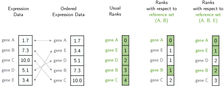
Figure 1: Example of ranking gene expression data with respect to a reference set.

Given a vector of gene expression levels $\mathbf{x}\in\mathbb{R}^{d},$ the rank of gene $j$, as understood in the common sense, can be obtained by counting the number of genes $k$ (among all $d$ genes) that are less expressed than gene $j$ (i.e. $x_{k}<x_{j}$).

We introduce a more general notion of rank, the rank $r_{j}^{\Gamma}$ of $x_{j}$ relative to a reference set $\Gamma$, by:

$$r_{j}^{\Gamma} =\sum_{k=1}^{d}{\mathbf{1}\!\left[k\in\Gamma\right]\mathbf{1}\!\left[x_{j}>x_{k}\right]}$$ (1)

Note that we clearly recover the classical rank in the particular case where $\Gamma=\{1,\ldots,d\}.$

In this paper, we will encode the set $\Gamma$ by a vector $\boldsymbol{\gamma}\in\{0,1\}^{d}$ with $\gamma_{j}=\mathbf{1}\!\left[j\in\Gamma\right].$ We can thus express $r_{j}^{\Gamma}$ as $r_{j}^{\Gamma}=\sum_{k=1}^{d}{\gamma_{k}\,\mathbf{1}\!\left[x_{j}>x_{k}\right]}.$ To simplify notations we will also drop the exponent $\Gamma,$ which will be defined from the context.

Now, to define simultaneously all the ranks associated with the elements of a vector $\mathbf{x}_{i}$ we introduce the matrix of binary comparisons $\mathbf{C}^{i}\in\mathbb{R}^{d\times d},$ with $\mathbf{C}^{i}_{jk}=\mathbf{1}\!\left[x_{ij}>x_{ik}\right].$ The vector of ranks $\mathbf{r}_{i}$ associated with a reference set encoded by the indicator vector $\boldsymbol{\gamma}$ is computed as $\mathbf{r}_{i}=\mathbf{C}^{i}\boldsymbol{\gamma}.$

We will use the index $i\in\{1,\dots,n\}$ to index the $n$ observations in the data.

2.2 Classification: learning the reference set along with a linear model on adaptive ranks

We consider a classical supervised learning problem in which input data is encoded as ranks $\mathbf{r}_{i}$ of the form above, and the output data is a label $y_{i}\in\mathcal{Y}$. For a loss function $\ell:\mathcal{Y}\times\mathbb{R}\rightarrow\mathbb{R}$, we consider a regularized empirical risk minimization of the form

$$\min_{\mathbf{w}\in\mathbb{R}^{d},\,b\in\mathbb{R}}{\textstyle\frac{1}{n}}\sum_{i=1}^{n}\ell(y_{i},\mathbf{w}^{\top}\mathbf{r}_{i}+b)+\Omega(\mathbf{w}),$$ (2)

where $\Omega$ is a (typically convex) regularizer. By expressing $\mathbf{r}_{i}$ as a function of $\boldsymbol{\gamma}$ and of $\mathbf{C}^{i}$ and minimizing the empirical risk with respect to $\boldsymbol{\gamma}$ as well, we propose to learn the reference set $\Gamma$.

This leads to the following optimization problem:

$$\min_{\boldsymbol{\gamma}\in\{0,1\}^{d},\,\mathbf{w}\in\mathbb{R}^{d},\,b\in\mathbb{R}}{\textstyle\frac{1}{n}}\sum_{i=1}^{n}\ell(y_{i},\mathbf{w}^{\top}\mathbf{C}^{i}\boldsymbol{\gamma}+b)+\Omega(\mathbf{w}).$$ (3)

Given that the integrality constraint on $\boldsymbol{\gamma}$ makes the optimization problem combinatorial, we propose to relax the constraint $\boldsymbol{\gamma}\in\{0,1\}^{d}$ to $\boldsymbol{\gamma}\in[0,1]^{d}$. We empirically found that adding a cardinality constraint on the reference set, ${\boldsymbol{\gamma}}^{\top}\mathbf{1}=s$ instead of penalizing with a sparsity inducing regularization, such as the $\ell_{1}$-norm, was useful to obtain fast convergence. We suppose that this constraint removes an indeterminacy of scale between $\mathbf{w}$ and $\boldsymbol{\gamma}$ which appears once the integrality constraint is removed, given that $(\alpha\,\mathbf{w},\frac{1}{\alpha}\,\boldsymbol{\gamma})$ yields identical losses values for any scaling factor $\alpha$; it would be implicitely removed as well by regularizers on $\mathbf{w}$ and $\boldsymbol{\gamma}$ but only at convergence.

Given the relaxed constraint $\boldsymbol{\gamma}\in[0,1]^{d}$, and in order to nonetheless obtain solutions with $\boldsymbol{\gamma}\in\{0,1\}^{d}$, we propose to solve a sequence of problems of the form

$$\min_{\boldsymbol{\gamma}\in[0,1]^{d},\,\mathbf{w}\in\mathbb{R}^{d},\,b\in\mathbb{R}}{\textstyle\frac{1}{n}}\sum_{i=1}^{n}\ell(y_{i},\mathbf{w}^{\top}\mathbf{C}^{i}\boldsymbol{\gamma}+b)+\Omega(\mathbf{w})+\lambda_{p}\,\rho(\boldsymbol{\gamma})\qquad\text{s.t.}\quad{\boldsymbol{\gamma}}^{\top}\mathbf{1}=s,$$ (4)

for an increasing sequence of regularization coefficients $\lambda_{p},$ where $\rho$ is the concave “push” penalty defined by

$$\rho(\boldsymbol{\gamma})=\sum_{j=1}^{d}\gamma_{j}(1-\gamma_{j}),$$ (5)

which effectively “pushes” the entries of $\boldsymbol{\gamma}$ towards the extreme points of the hypercube $[0,1]^{d}.$ More precisely, starting from $\lambda_{p}=0$, the solution of each problem in the sequence is used as initialization to warm-start the next one, and the sequence is terminated when the solution satisfies the constraint $\boldsymbol{\gamma}\in\{0,1\}^{d}$.

It is obviously possible to only solve the above problem for $\lambda_{p}=0$ and renounce the integrality constraints. Actually, the presence of the capped-simplex constraints $\boldsymbol{\gamma}\in[0,1]^{d}$ and $\boldsymbol{\gamma}^{\top}\mathbf{1}=s$ are themselves sufficient to obtain that, at the optimum, $\boldsymbol{\gamma}^{*}$ tends to lie on a lower dimensional face of the capped-simplex, so that a significant fraction of its entries are exactly equal to $0$ or $1$. In preliminary experiments, we also did not observe significant differences whether integrality constraints are strictly enforced or not. The main motivations to nonetheless enforce them, are that (a) the additional computational effort is small compared to the cost of solving the problem with $\lambda_{p}=0,$ (b) the interpretability of the obtained ranks is otherwise lost, and (c) that it tends to produce slightly sparser solutions.

3 Optimization procedure

Block proximal coordinate descent.

When $\lambda_{p}=0,$ problem (4) is bi-convex. More precisely, the objective function to minimize, which we denote by $\mathcal{O}(\lambda_{p};\boldsymbol{\gamma},\mathbf{w},b)$, is convex w.r.t. $(\mathbf{w},b)$ when $\boldsymbol{\gamma}$ is fixed and convex w.r.t. $(\boldsymbol{\gamma},b)$ when $\mathbf{w}$ is fixed. This suggests that a form of alternating descent algorithm can be used, such as block coordinate descent, in which blocks of variables, here $(\boldsymbol{\gamma},b)$ and $(\mathbf{w},b)$, are alternatively updated (see for example Tseng and Yun,, 2009; Xu and Yin,, 2013).
In addition, since the regularizer $\Omega$ is convex and potentially non-differentiable (e.g., elastic net regularization), descent w.r.t. $\mathbf{w}$ can be suitably realized with proximal gradient steps, provided that the proximal operator for $\Omega$ can be computed efficiently. For $\gamma$, the optimization step satisfying the constraint $\boldsymbol{\gamma}\in[0,1]^{d}\mid\boldsymbol{\gamma}^{\top}\mathbf{1}=s$ also involves a proximal operator: the projection on this constraint set called capped-simplex. We derive this proximal operator in Appendix B.1.
Therefore, to solve each instance of problem (4), we use a block proximal coordinate descent algorithm (BPCD). Shi et al., (2014) propose a BPCD algorithm to solve bilinear logistic regression problems with convex regularizers. Our implementation is similar to theirs, except that we use different blocks and a simpler stopping criterion, which is better suited to the non-convexity of the push-penalty and to the implementation of the path-following algorithm described next. We detail our implementation in Appendix B.3.

Initialization.

Given that the optimization problem is non-convex, the initialization matters: for reasons of symmetry we set $\mathbf{w}=\mathbf{0}$ and $\boldsymbol{\gamma}=\frac{s}{d}\mathbf{1},$ i.e., the center of the capped-simplex.

Path-following algorithm.

Concerning the sequence of values of $\lambda_{p}$ used for the problems of the form (4), given that the term $\lambda_{p}\hskip 0.5pt\rho$  eventually creates local minima at all vertices of the capped-simplex, it is important not to increase $\lambda_{p}$ too quickly, which could produce suboptimal solutions. We use the approach proposed by Zaslavskiy et al., (2009). In essence, we adjust the next $\lambda_{p}$ to ensure a sufficiently small increase of the objective value $\mathcal{O}$ for the previously found solution. The strategy is detailed in Appendix B.4.

To summarize, we propose to solve each instance of problem (4) with a block proximal coordinate descent algorithm (BPCD), and to increase $\lambda_{p}$ according to a rule inspired by the path-following algorithm in Zaslavskiy et al., (2009). This scheme is summarized in Algorithm 1.

Algorithm 1 Optimization Procedure

$\gamma\leftarrow\frac{s}{d}\mathbf{1}$,  $\mathbf{w}\leftarrow\mathbf{0}$,   $\lambda_{p}=0$ $\triangleright$ Initialization

while $\boldsymbol{\gamma}\notin\{0,1\}^{d}$ do $\triangleright$ Iterating on $\lambda_{p}$

     $(\boldsymbol{\gamma},\mathbf{w},b)\leftarrow\operatorname*{argmin}_{\boldsymbol{\gamma}\in[0,1]^{d},\,\boldsymbol{\gamma}^{\top}\mathbf{1}=s,\,\mathbf{w}\in\mathbb{R}^{d},\,b\in\mathbb{R}}\mathcal{O}(\lambda_{p};\boldsymbol{\gamma},\mathbf{w},b)$ $\triangleright$ solved with BPCD

     $\lambda_{p}\leftarrow\lambda_{p}^{\prime}$ , with $\mathcal{O}(\lambda_{p}^{\prime};\boldsymbol{\gamma},\mathbf{w},b)-\mathcal{O}(\lambda_{p};\boldsymbol{\gamma},\mathbf{w},b)=\epsilon$.

end while

return $\boldsymbol{\gamma},\mathbf{w},b$

Note.

When $\lambda_{p}>0$, although $\rho$ is non-convex, problem (4) can still be formulated as a multi-convex problem, suitable to the block coordinate descent (see Appendix B.2 for a derivation).

3.1 Computing the product $\mathbf{C}^{i}\boldsymbol{\gamma}$ with complexity $O(d)$.

A priori, the computation of the matrix vector product $\mathbf{C}^{i}\boldsymbol{\gamma}$ involves $d^{2}$ multiplications. But it is clear that to compute classical ranks it is sufficient to sort the data, which can be done with a complexity of $O(d\log d).$ Since $\mathbf{C}^{i}\boldsymbol{\gamma}$ is none else than the vector of ranks with respect to the reference set $\Gamma,$ it seems reasonable to think that the same complexity can be achieved, and this is indeed the case. Assuming that there are no ties, and if $\sigma_{i}$ is a permutation sorting the entries of $\mathbf{x}_{i}$, i.e.  such that $x_{i,\sigma_{i}(1)}<\dots<x_{i,\sigma_{i}(d)}$, the inner-sum can be calculated recursively by applying the same permutation to $\boldsymbol{\gamma}$ and applying, from $j=1$ to $d$,

$$r_{i,\sigma_{i}(j)}\leftarrow r_{i,\sigma_{i}(j-1)}+\gamma_{\sigma_{i}(j-1)},$$ (6)

with, by convention, $r_{i,\sigma_{i}(0)}=0.$
The complexity is therefore dominated by the sorting operation and is thus $O(d\log d)$. Moreover, sorting the data needs to be done only once at the beginning of the optimization, so that effectively the number of operation needed to compute $\mathbf{C}^{i}\boldsymbol{\gamma}$ each time $\boldsymbol{\gamma}$ is updated is $O(d).$ The exact same reasoning applies to the computation of $\mathbf{w}^{\top}\mathbf{C}^{i}$ which is therefore also $O(d),$ once the inverse of $\sigma_{i}$ is computed. With the alternative definitions of rank and in the presence of ties, the calculations are more subtle, but the same complexity can be obtained. They are detailed in Appendix A.2.

4 Benchmark: competing classification algorithms

We will apply the proposed methodology to solve a number of binary classification problems on first synthetic and then real RNA-Seq data. To serve as a basis of comparison, we choose standard logistic regression or random forest classifiers that rely either on a rank representation or not.

Optirank: a sparse rank-based logistic regression with learnable reference set.

To solve binary classification tasks, we propose optirank, a logistic regression model on rank-transformed data, with ranks computed with respect to a learnable reference set. Our model optirank is fitted within the framework introduced in section 2.2, by solving the optimization problem (3) with a logistic loss $\ell(y,a)=-y\log{(S(a))}-(1-y)\log{(1-S(a))}$, where $S(x)$ denotes the sigmoid function $S(x)=1/(1+e^{-x}),$ $y\in\mathcal{Y}=\{0,1\}$ being the binary label, and with an elastic net regularization

$$\Omega(\mathbf{w})=\lambda_{1}\,\left\lVert\mathbf{w}\right\rVert_{1}+\lambda_{2}\,\left\lVert\mathbf{w}\right\rVert_{2}^{2},$$

to induce sparsity in the set of features whose rank is relevant to the classification task. In fact, given that we consider RNA-Seq data, and that there are potentially significant correlations between genes, the use of the elastic net, with a Euclidean regularization on top of the Lasso terms, aims at stabilizing feature selection (see Zou and Hastie,, 2005).

Competing algorithms.

We will compare our optirank  algorithm with classical logistic regression (lr) equipped with the same elastic net regularization $\Omega$, and logistic regression on rank-transformed data (rank-lr), still with the same regularization. In addition, in tasks involving real data, we will also compare our method to the random forest (rf) and to the SingleCellNet algorithm (SCN) proposed by Tan and Cahan, (2019) for cell-typing tasks that we consider in our benchmark (see Section 6). The SCN algorithm consists of a pre-processing pipeline which identifies gene pairs with informative differential expression and transforms the RNA-Seq data into a binary matrix indicating the order of gene pairs followed by a random forest classifier.

Implementation details.

The stopping criterion in the scikit-learn (Pedregosa et al.,, 2011) implementation of logistic regression being different from the one in optirank, to ensure that this discrepancy does not affect the comparison on real datasets, we re-optimize the weights $\mathbf{w}$ learned by optirank  with the logistic regression of scikit-learn. Additional details about the classifiers can be found in Appendix C.

5 A synthetic data distribution model with unstable ranks

In order to illustrate the potential and limitations of optirank, we present in the following a synthetic example in which the robustness of the rank normalization is challenged. We test whether optirank is effectively able to overcome the difficulty of the task.

5.1 Model

As mentioned in Lausser et al., (2016), the strength of rank-normalization can be linked to the fact that ranks are invariant to observation-wise monotone perturbations of the gene expressions. Those perturbations can be easily envisioned, for example by considering that counts depend in a quadratic (and observation-dependent) fashion on the RNA content in the observation. By contrast, the following example focuses on a weakness of rank normalization that arises in the presence of a non-monotone, nonetheless simple, perturbation. Those perturbations occur in real data; for instance, Leek et al., (2010) report a case in which a group of genes shifts between different batches of samples. In our example, we consider a similar perturbation: we suppose that there is a group of perturbed genes, uninformative for the classification task at hand, that introduces noise in the ranks of relevant features by fluctuating in a coordinated and observation-wise manner.

More precisely, the expression levels of the genes in this group, called $P$, are all assumed to shift by an additive amount close to $\Delta_{i}$ (unique to the observation $i$). This introduces noise in the ranking of the other stable genes: indeed, since the perturbed genes in $P$ shift in a coordinated fashion, the rank of a stable gene is increased or decreased by an amount proportional to the number of genes in $P$ that cross it.

We propose the following synthetic model: the non-perturbed expression of a gene $j$ in observation $i$, $\widetilde{X}_{ij}$, follows a Gaussian distribution centered on the typical expression value of gene $j$, $\mu_{j}$:

$$\widetilde{X}_{ij}\sim\mathcal{N}(\mu_{j},\sigma^{2})\,,$$ (7)

where $\sigma$ defines the magnitude of the baseline noise in the data. We generate values for $\mu_{j}$ by sampling uniformly on the expression interval, which we set to $\left[0,1\right]$.
The expression of a perturbed gene in $P$ is generated by adding to the unperturbed expression $\widetilde{X}_{ij}$ an observation-wise shift $\Delta_{i}$ that we sample from a centered Gaussian distribution $\mathcal{N}(0,\tau^{2})$, with $\tau$ defining the typical magnitude of the perturbation. Summing all contributions, the expression of a gene $j$ in observation $i$, $X_{ij}$, is generated as:

$$X_{ij}=\begin{cases}\widetilde{X}_{ij}+\Delta_{i}&\text{if }j\in P\\ \widetilde{X}_{ij}&\text{otherwise.}\end{cases}$$ (8)

Finally, we assign to each observation $i$ a label generated from a simple logistic model on the ranks within the stable (non-perturbed) genes (forming the set $S$):

$$\mathbb{P}(Y=1|X=\mathbf{x})=\sigma(\mathbf{w}^{\top}\mathbf{r}^{\Gamma}+b),\quad\text{with}\quad w_{j}=0,\;\forall j\notin S\quad\text{and}\quad\Gamma=S.$$ (9)

The generation of the parameters $\mathbf{w}$, $\boldsymbol{\gamma}$, and $b$ is detailed in Appendix D.

5.2 Results

We benchmarked on this synthetic data three different classifiers based on logistic regression: the simple logistic regression (lr), the logistic regression on ranked data (rank-lr), and optirank, which can produce the rank-lr model as a particular case but offers the additional flexibility of restraining the reference set. Concerning the choice of regularization hyperparameters, note that we tuned only the ridge regularization coefficient $\lambda_{2}$ (and $s$ for optirank), setting the lasso penalty $\lambda_{1}$ to zero for all three classifiers, given that we consider sample sizes $n$ that are large compared to the number of variables $d$.

With default simulation parameters, optirank  outperforms both rank-lr and lr (see Table  1). Moreover, optirank  is empirically able to recover the true reference set. Indeed, the cosine similarity $S_{C}$ between the vector $\boldsymbol{\gamma}$ used to generate the data (see equation 9) and the one found by optirank  is high: $S_{C}=0.95\pm 0.03$.

	Test Balanced Accuracy ($\%$)
Logistic Regression (lr)	$78\pm 2$
Logistic Regression on Full Ranks (rank-lr)	$80\pm 3$
optirank (our model)	$96\pm 0.4$

Table 1: Test balanced accuracy (in $\%$) for classifiers on the synthetic example of Section 5. Default simulation parameters were set to $d=50$, $d_{P}=40$, $n=1000$, $\tau=0.2$, and $\sigma=0.05$.

We investigated how this comparison evolves when we change the number of perturbed genes $d_{P}$ or the dimension of the gene expression profile $d$, while maintaining the ratio between the number of observations and the dimension ($n/d$) fixed. Not surprisingly, the superiority of optirank over lr and rank-lr fades when the number of perturbed genes $d_{P}$ becomes small relative to the dimension of the gene expression profile. Indeed, Figure 2 shows that when $d$ increases while keeping the number of perturbed genes, $d_{P}$, equal to 40 , rank-lr and lr scores rise to the level of optirank (whose performance degrades slightly). In accordance, when the number of perturbed genes is increased while keeping the dimension of the gene expression to 50, the performance of rank-lr and lr degrades, while the score of optirank remains high. This outlines the fact that the perturbation on the usual ranks of informative genes becomes smaller as the ratio $d_{P}/d$ decreases.

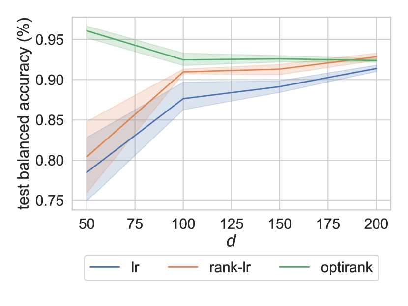
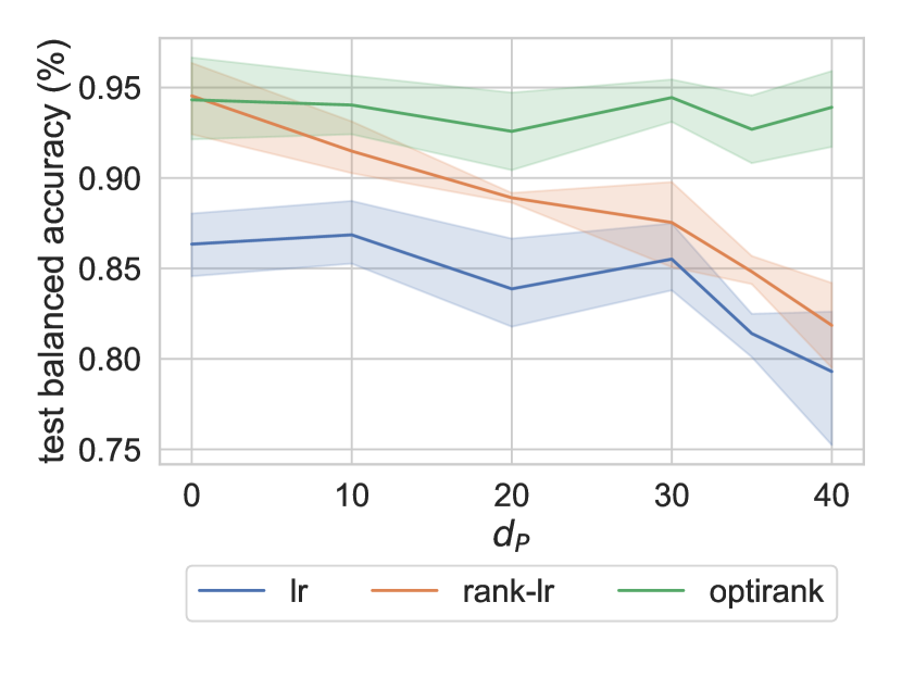
Figure 2: Dependence of the test-accuracy with respect to the dimension of the gene expression profile $d$ when $d_{P}=40$, and with respect to the number of perturbed genes $d_{P}$ for $d=50$. The shaded area shows the standard error across runs.

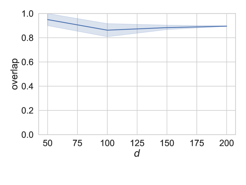
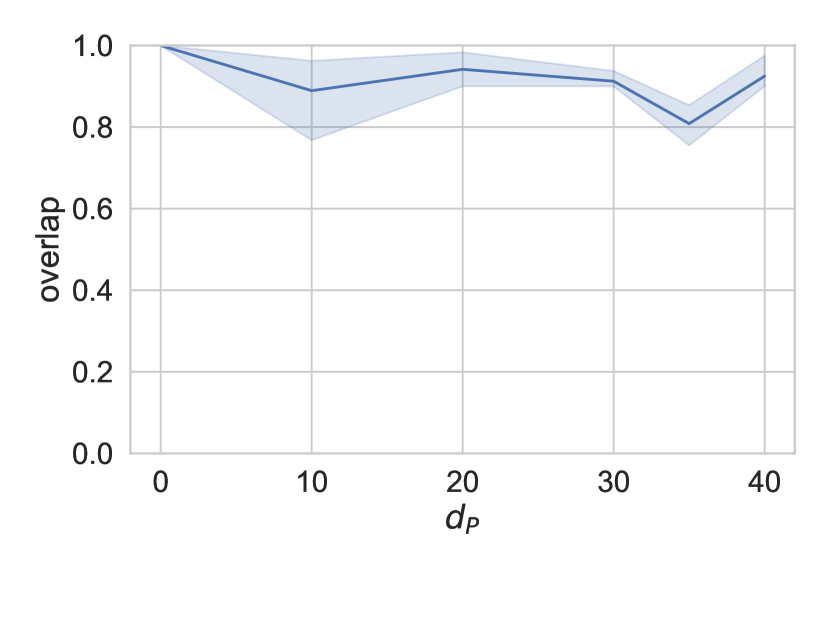
Figure 4: Cosine similarity $C_{S}$ between the true $\gamma$ and the one fitted by optirank, as a function of the dimension $d$ and the number of perturbed genes $d_{P}$. The shaded area shows the standard error across runs. Default simulation parameters were set to $d=50$, $d_{P}=40$, $n=1000$, $\tau=0.2$, and $\sigma=0.05$.

Concerning the cosine similarity between the ground truth reference set and the reference set found by optirank, its dependence on the simulation parameters $d_{P}$ and $d$ is small: Figure 4 in Appendix D.3 shows that the overlap remains high.

For the dependence of scores on $\tau$, which defines the magnitude of the observation-wise shift $\Delta_{i}$, see Figure 3 in Appendix D.3.

In summary, this synthetic task exemplifies (a) how a non-monotone perturbation can effectively degrade the performance of the rank normalization, and (b) that optirank is robust to the kind of perturbation introduced thanks to its learnable ranking reference set.

6 Experiments on real RNA-Seq data

In this section, we benchmark optirank on multiple biologically relevant classification tasks with real RNA-Seq data. These tasks present qualitatively different dataset shifts between train and test data. In Subsection 6.1, we evaluate how robust different algorithms are to these dataset shifts. To enhance robustness, we then investigate in Subsection 6.2, an alternative learning scenario in which multiple source datasets are merged in the training data. In this manner, we hope that the algorithm learns better to be robust to the kind of perturbation it will encounter in the test data.

6.1 Classification with different dataset shifts

6.1.1 Classification tasks

CUP-related tasks.

Cancer of unknown primary (CUP) occurs when a patient has a metastatic tumor whose organ of origin (where the primary tumor was located) cannot be determined. A lot of effort has been dedicated to develop classifiers to predict the organ of the primary tumor based on RNA-Seq data of the metastatic tissue, in the hope of personalizing and enhancing the treatment given to CUP patients (Laprovitera et al.,, 2021). However, an obstacle in building efficiently such classifiers is the scarsity of RNA-Seq data of metastatic tumors. As a result, classifiers are often trained and tuned on datasets of primary tumors, which are biologically different from metastasis, and metastatic samples are reserved to the external classifier validation. This is precisely what we do in the three tasks TCGA, PCAWG, met500. In the task TCGA, classifiers are trained on the TCGA dataset comprising primary tumors (The Cancer Genome Atlas Research Network et al.,, 2008), and tested on a held out portion of the same dataset. In the task PCAWG, those same classifiers trained on TCGA were tested on an external dataset PCAWG also with primary tumors (The ICGC/TCGA Pan-Cancer Analysis of Whole Genomes Consortium,, 2020). Finally, the task met500 evaluates those classifiers on the met500 dataset (published by Leiserson et al.,, 2015), which comprises metastatic tumors of various origins. The two latter tasks represent different challenges in terms of dataset-shift between train and test. The task PCAWG is subject to technical variation between two separately obtained datasets, which we call batch-effect. An additional difficulty in the met500 task is that a metastasis differs biologically from its primary tumor, resulting in a so-called biologically induced dataset shift.

Cell-typing single-cell data.

Single-cell RNA-Seq (scRNA-Seq) provides a way to probe gene expression at the cell-level resolution. A preliminary step in single cell data analysis resides in the cell-type identification of each observation/cell, i.e. cell typing. To achieve this automatically, Tan and Cahan, (2019) propose to train a classifier on a labeled dataset comprising many cell types — commonly known as a cell-atlas, and use it to infer the cell-types in an unlabelled dataset. One difficulty is that the train and test scRNA-Seq data are potentially generated by different sequencing platforms. Tan and Cahan, (2019) evaluate the robustness of their classifier SCN for various cross-platform train and test data combinations (Tasks Baron-Murano, Baron-Segerstolpe, MWS-TM10x, MWS-TMfacs, TM10x-MWS, TM10x-TMfacs and TMfacs-MWS). We use the same tasks to investigate the usefulness of optirank in counteracting dataset shifts induced by different sequencing platforms and compare with the original method SCN.

BRCA task.

The task BRCA consists in predicting the presence of the BRCA mutation from the RNA-Seq data in breast primary tumors from the TCGA dataset. This task does not directly answer a real-life classification problem. However, the classifier coefficients could be used to obtain a (sparse) transcriptional signature for BRCA cancer.

We list all tasks while grouping them by type of dataset shift (if any) between the train and test data in Table 2.

Dataset-shift	Tasks
None (same distribution)	BRCA, TCGA
Batch-effects	PCAWG
Technical dataset-shift (Different sequencing platforms)	Baron-Murano, Baron-Segerstolpe, MWS-TM10x, MWS-TMfacs, TM10x-MWS, TM10x-TMfacs and TMfacs-MWS
Biologically induced dataset-shift	met500

Table 2: Classification tasks by type of dataset-shift between train and test set.

Additional details about the data sources are in Appendix E.1.

6.1.2 Data pre-processing

For fairness of comparison and as first step of dimensionality reduction, the data was reduced to include the 1000 genes occuring in informative pairs identified by SCN. Logged raw-cpm values were used as input for each classifier (see Appendix E.2 for additional details).

6.1.3 Hyperparameter selection

The $\ell_{1}$ and $\ell_{2}$ regularization coefficients of optirank, lr  and  rank-lr , and the $s/d$ ratio for optirank  were tuned via internal cross-validation (i.e., using held out data from the same source as the training data; see Appendix E.3.1, E.3.2 and E.4 for details). SingleCellNet was used with parameters suggested by Tan and Cahan, (2019), and random forest (rf) was trained with $300$ trees. Optimal hyperparameters were chosen with the one-standard error rule (Hastie et al.,, 2015) which selects the sparsest model with a score within one standard error of the best one.

6.1.4 Results and discussion

The performance in terms of balanced accuracy of all classifiers on the different classification tasks presented in Section 6.1.1 are summarized in the following table (Table 3). We highlighted in bold the scores of classifiers that did not score significantly worse than the winning method, according to a paired Student’s t-test.

	SCN	lr	optirank	rank-lr	rf
BRCA	$50.1\pm 0.3$ (4)	$\mathbf{58\pm 2}$ (1)	$52\pm 2$ (3)	$\mathbf{53\pm 1}$ (2)	$50.0\pm 0$ (5)
TCGA	$92\pm 1$ (5)	$\mathbf{99.14\pm 0.23}$ (2)	$\mathbf{99.06\pm 0.26}$ (3)	$\mathbf{99.3\pm 0.3}$ (1)	$95.7\pm 0.5$ (4)
PCAWG	$\mathbf{76.0\pm 4.5}$ (2)	$\mathbf{76.2\pm 5.4}$ (1)	$\mathbf{74.3\pm 5.4}$ (4)	$\mathbf{74.4\pm 5.8}$ (3)	$60\pm 4$ (5)
met-500	$67\pm 4$ (4)	$71\pm 4$ (3)	$\mathbf{77\pm 4}$ (1)	$\mathbf{75\pm 4}$ (2)	$60\pm 4$ (5)
Baron-Murano	$89\pm 2$ (3)	$87\pm 3$ (4)	$\mathbf{93.0\pm 1.9}$ (2)	$\mathbf{93.2\pm 1.9}$ (1)	$62\pm 3$ (5)
Baron-Segerstolpe	$\mathbf{93.5\pm 1.6}$ (3)	$\mathbf{93.4\pm 2.2}$ (4)	$\mathbf{93.6\pm 2.2}$ (2)	$\mathbf{94.0\pm 1.8}$ (1)	$60\pm 3$ (5)
MWS-TM10x	$72\pm 2$ (4)	$\mathbf{86\pm 2}$ (1)	$\mathbf{84\pm 2}$ (3)	$\mathbf{85\pm 2}$ (2)	$53\pm 1$ (5)
MWS-TMfacs	$70\pm 2$ (4)	$\mathbf{86\pm 1}$ (3)	$\mathbf{87.3\pm 1.6}$ (2)	$\mathbf{87.4\pm 1.7}$ (1)	$50.01\pm 0.01$ (5)
TM10x-MWS	$51.5\pm 0.3$ (4)	$\mathbf{72\pm 2}$ (1)	$65\pm 2$ (2)	$63\pm 2$ (3)	$51.0\pm 0.2$ (5)
TM10x-TMfacs	$80\pm 1$ (4)	$91\pm 1$ (3)	$\mathbf{92.3\pm 0.9}$ (2)	$\mathbf{92.7\pm 0.9}$ (1)	$58\pm 1$ (5)
TMfacs-MWS	$51.0\pm 0.2$ (4)	$\mathbf{71\pm 2}$ (1)	$64\pm 1$ (3)	$66\pm 2$ (2)	$50.2\pm 0.1$ (5)

Table 3: Average balanced accuracies in % (across folds and classes) of competing classifiers on the different tasks detailed in Section 4. Horizontal lines separate tasks with different types of dataset shift, from top to bottom: generalization to the same distribution, robustness to batch-effects, robustness to biologically-induced dataset shifts and robustness across sequencing platforms. The integer in parenthesis denotes the rank of the classifiers in terms of average balanced accuracy (lower is better). Classifiers which did not score significantly worse than the best classifier according to a paired Student’s t-test (with a level of 5 %) are highlighted in bold (see Appendix E.5 for additional details).

Interestingly, the advantage of logistic regression-based classifiers relying on a rank-representation (optirank, rank-lr) over their non-ranked counterpart (lr) is not consistent, but rather depends on the task considered. Indeed, on the tasks TM10x-MWS and TMfacs-MWS, lr clearly surpasses its ranked counterparts, while on the tasks met500, Baron-Murano and TM10x-TMfacs we notice the opposite trend. This indicates that the rank representation confers additional robustness against dataset shifts only in some instances.

A burning question is whether there is an advantage of ranking relative to a subset of genes compared to ranking among all. At first sight, this doesn’t seem to be the case: the performances of optirank and rank-lr are similar. In a more thorough analysis in which we carried paired Student’s t-tests for every task and every pair of classifiers (see Appendix E.5), only the task TM10x-MWS showed a significant difference between rank-lr and optirank, in favor of optirank.

In summary, in these tasks, the ranking reference set found by optirank is not more robust than the classical full reference set. A possible explanation is that an optimal restricted reference set does not necessarily exist. Contrarily to the synthetic example in Section 5 and to certain observations made on real data (see Leek et al.,, 2010), where a group of genes shift in one direction and perturb the ranking, in the tasks we consider, the dataset-shift could either be a monotone transformation or could shift genes in opposite directions. In both these scenarios, the ranks of certain stable genes would not be affected by the dataset shift. Alternatively, one could argue that even if such an optimal restricted reference set existed, the only way to discover it would be by inspecting the test dataset. We address this question in an additional experiment presented in the next section.

Aside from the performance aspect, it is important to note that by definition, the classical ranking normalization is computed with the measurement of all (reference) genes. In contrast, optirank can find models that require only a small number of genes to be sequenced, which can be a decisive advantage in some medical applications. In the tasks we consider, solutions found by optirank require around 500 genes, half of the thousand used by rank-lr. However, it is worth noting that when the logistic regression performs well, there is no advantage of using optirank, as the latter tends to produce less sparse solutions (see Appendix E.5.6).

It is worth noting that in general, the random forest rf performs worse than other classifiers, and that SCN does not provide a competitive advantage on single-cell typing tasks.

6.2 Enhancing robustness with a multi-source learning scenario

In this experiment, we investigate whether in the presence of dataset shifts, merging two source datasets in the training set increases the classification accuracy on the third external target dataset. The rationale is that the algorithm could learn to be robust to the kind of perturbation it will encounter in the target dataset.
To achieve this, we constructed three tasks: TCGA-PCAWG-met500, Baron-Segerstolpe-Murano and MWS-TMfacs-TM10x. The tasks are named after the datasets that compose them: the first is the main source dataset, the second the auxiliary source dataset and the third is the target dataset. We compare the performance in the multi-source scenario (where the main and auxiliary source datasets are merged into a training set) to a baseline scenario in which the auxiliary source dataset is not used (single-source scenario). Appendix E.3.2 provides additional details about the construction of those tasks.

ANrank-lr.

One could ask if, with the help of the auxiliary source dataset, robust ranking reference genes can be identified in a simpler manner than in optirank, in particular, with a selection step decoupled from the fitting process. To answer this question, we constructed an additional logistic regression classifier based on adaptive ranks, ANrank-lr, that selects the ranking reference genes based on a simple ANOVA test. For each gene, the vulnerability to dataset-shift is assessed with a two-way ANOVA which determines the effect of label and dataset jointly. The $s$ most robust genes are selected as ranking reference (See Appendix C.6 for additional details). For completeness, we evaluate ANrank-lr both in the multi-source and in the single-source scenario. In the single-source setting, ANrank-lr uses the auxiliary source dataset only for the ANOVA test (and not during fitting nor validation).

Data preprocessing and hyperparameter selection.

Data preprocessing was done as described in the previous section. Appendix E.3.2 details the procedure to obtain the cross-validation splits: special care was taken to have similar training dataset sizes in the multi-source and single-source scenarios. The hyperparameter grids used for cross-validation are the same as in the previous experiment. Concerning ANrank-lr, the number of ranking reference genes $s$ and the elastic net regularization coefficients are tuned over the same grid as for optirank.

6.2.1 Results and Discussion.

There is a clear benefit brought by merging two source datasets in the training phase (multi-source scenario). Indeed, for nearly all classifiers and tasks, the average balanced accuracy is greatly increased in the multi-source scenario (Table 4) compared to the single-source scenario in which the auxiliary source dataset is not used (see Table 25 in Appendix E.5.8). Accordingly, for both single-cell typing tasks, the leading score is greater in the multi-source scenario than in the single-source scenario. Moreover, the regression classifiers based on ranks (optirank, ANrank-lr, and rank-lr) outperform the simple logistic regression (lr).

However, as in the previous section, the performances of optirank and rank-lr seem comparable: in the single-cell tasks, the paired t-tests do not reveal any significant difference between the two classifiers (see Appendix E.5).

It is worth noting that despite the simplicity of its method for restricting the reference set, ANrank-lr reaches a level of performance comparable with the other ranked-based algorithms, in particular optirank, and likewise outperforms the simple logistic regression. This is particularly interesting since, by definition, ANrank-lr can produce sparse solutions. Indeed, in Appendix E.5.7, we note that optirank and ANrank-lr find solutions involving a similar number of genes. In accordance with the results of the previous section, the simple logistic regression produces substantially sparser solutions.

	ANrank-lr	SCN	lr	optirank	rank-lr	rf
TCGA-PCAWG-met500	$\mathbf{81\pm 4}$ (1)	$69\pm 5$ (4)	$\mathbf{80\pm 4}$ (2)	$68\pm 4$ (5)	$71\pm 4$ (3)	$65\pm 4$ (6)
Baron-Segerstolpe-Murano	$98.0\pm 0.3$ (3)	$93.2\pm 0.8$ (5)	$97.2\pm 0.4$ (4)	$\mathbf{98.1\pm 0.3}$ (2)	$\mathbf{98.2\pm 0.3}$ (1)	$67\pm 3$ (6)
MWS-TMfacs-TM10x	$\mathbf{95.63\pm 0.40}$ (3)	$83\pm 1$ (5)	$92.5\pm 0.9$ (4)	$\mathbf{95.64\pm 0.41}$ (2)	$\mathbf{95.9\pm 0.4}$ (1)	$72\pm 2$ (6)

Table 4: Multi-source scenario. Average balanced accuracies in % (across folds and classes) of competing classifiers on the tasks detailed in section 6.2 in the case in which the first two source datasets are merged in the training phase. The integer in parenthesis denotes the rank of the classifiers in terms of average balanced accuracy (lower is better). Classifiers which did not score significantly worse than the best classifier according to a paired Student’s t-test are highlighted in bold (see App. E.5 for additional details).

Runtime comparison.

The runtime for competing classifiers was measured in the previous single-source scenario. Table 26 in Appendix E.5.9 attests that the fitting time of both optirank and ANrank-lr are reasonable and in some instances lower than the one of their competitors.

Conclusion

According to the literature, rank normalization confers increased robustness against distribution shifts that occur in RNA-Seq data. This success is linked to the fact that rank normalization is invariant to all perturbing monotone transformations that occur between different datasets and/or samples. However, a potential weakness of using rank normalization is that the rank of genes that might be biologically relevant can be perturbed by fluctuations of irrelevant ones.
To counteract this problem, we proposed optirank, an algorithm that learns a ranking relative to an optimal reference genes set while learning a classification or regression model. We showed on a synthetic example, inspired by observations on real data, how rank-normalization can suffer from collective fluctuations of an ensemble of genes that perturb the ranks, and demonstrated the ability of optirank to eliminate those genes from the ranking reference set, thereby allowing it to solve successfully the classification task.

We then assessed the performance of optirank on 11 real classification tasks, presenting different challenges in terms of distribution shifts occurring between train and test data. Indeed, we hypothesize that our model is able in some instances to remove from the ranking reference set genes that have the propensity to shift in the test distribution, thereby perturbing the ranks learned on the training data. Firstly, we observed that the advantage of the rank transformation is not systematic. Moreover, contrary to our hypothesis, restricting the reference set, as is done by optirank, does not seem to provide increased robustness compared to ranking relative to the full set of genes.

As an additional way to tackle distribution shifts occurring between train and test data, we propose a multi-source learning scheme. In this scheme, we train a classifier on a union of two different datasets in which a dataset shift occurs, hoping to make it more robust and efficient on a third external dataset. We show that this scenario is particularly useful in the cell-typing tasks, in particular when used in synergy with rank-based classifiers. We also explored an alternative way of restricting the reference set, with a simple ANOVA test that exploits the multiple sources in the training data. Despite its simplicity, the resulting classifier, which we call ANrank-lr, achieves a level of performance similar to optirank.

Finally, it is important to mention that restricting the reference set reduces the number of genes needed to be sequenced, while maintaining the level of robustness and accuracy of the rank normalization. Therefore, in certain medical applications where sparsity is desired, it can be worth considering the classifiers optirank and ANrank-lr.

7 Code and Data Availability

The code and the data necessary to reproduce the results are available on the Github repository https://github.com/paolamalsot/optirank.

Appendix A Notions of rank in the presence of ties

For the RNA-Seq data we consider in several experiments, the read count of a few genes are equal to $0$. This leads to ties between these genes, which motivated us to extend the formulation proposed to that case.

A.1 Different rank definitions

Ever since ranks were introduced in statistics, there have been discussions on how to correctly treat ties (Kendall,, 1945). For more references and discussion on recent related work, we refer the reader to Amerise and Tarsitano, (2015).

The three simplest approaches, and the ones which could be relevant in our setting, consist in assigning to a group of tied genes whose ties are initially broken arbitrarily, respectively their minimum, maximum, or average rank.

For simplicity, and given that the problem of ties is not central to the set of ideas that we are presenting and might be irrelevant in many cases, the generalization of classical ranks to ranks with respect to reference set that we introduce in the paper stems from the minimum rank definition. However, our implementation of the optirank algorithm uses the better behaved average rank.

We propose in the following generalizations of these different ranks to the case where ranks are defined with respect to a reference set $\Gamma.$

Minimum rank.

In Section 2.1 we introduced the following definition of rank $r_{j}^{\Gamma}$ of $x_{j}$ relative to a reference set $\Gamma$:

$$r_{j}^{\Gamma} =\sum_{k=1}^{d}{\mathbf{1}\!\left[k\in\Gamma\right]\mathbf{1}\!\left[x_{j}>x_{k}\right]}\;.$$ (10)

The above definition of ranks assigns to tied values the minimum rank they would have if they were arbitrarily ordered, hence the name of minimum rank. This rank is also referred to as the standard competition rank for obvious reasons. Note that with the mathematical definition above, the smallest rank equals $0$; to obtain ranks that starts at $1$ it suffices to add $1$ to all rank values.

Average rank.

A way of handling ties which has better properties, in particular which keeps constant the sum of the ranks, is to assign to them the average value of these ranks, hence the name average ranking. In mathematical terms, this is:

$$r_{i}^{\Gamma} =\sum_{j=1}^{d}{\mathbf{1}\!\left[j\in\Gamma\right]\left(\mathbf{1}\!\left[x_{i}>x_{j}\right]+0.5\,\mathbf{1}\!\left[x_{i}=x_{j}\right]\right)}-0.5$$ (11)

$$=\sum_{j=1}^{d}{\gamma_{j}\left(\mathbf{1}\!\left[x_{i}>x_{j}\right]+0.5\,\mathbf{1}\!\left[x_{i}=x_{j}\right]\right)}-0.5\,,$$ (12)

where the offset of $0.5$ sets again the lowest rank to the value of $0$. (The fact that this offset appears here while it did not appear for the minimum rank could seem surprising, but it is necessary because we sum over all values of $j$ including $j=i$.) Again to obtain ranks that starts at $1$ we can add $1$ to all ranks. The average rank is also sometimes called the fractional rank.

Maximum rank.

Yet another possible definition, which is symmetric with the minimum rank, consists in replacing the strict inequality in (10) by an inclusive inequality and adding an offset of $1$ (to keep our convention that the ranks start at $0$). This results in:

$$r_{j}^{\Gamma} =\sum_{k=1}^{d}{\mathbf{1}\!\left[k\in\Gamma\right]\mathbf{1}\!\left[x_{j}\geq x_{k}\right]}-1\;.$$ (13)

The maximum rank is also called modified competition rank.

In our implementations and experiments, we systematically used the average rank for two main reasons. First, if two variables (i.e. genes in our case) have systematically close values (i.e. that are either equal or tend to be very close and in arbitrary order), we would expect the coefficients $w_{j}$ associated with their ranks in a classification model to be close. In that case, it is natural to request that the linear score does not change much whether they are exactly equal or not. Given that the sum of the ranks of tied values is constant for the average rank, it satisfies this property, which fails for the min and the max rank. Second, for a non-trivial reference set, and when there are no numerical ties, the average rank only assigns integer valued ranks for the elements of the reference set $\Gamma$, and any element falling exactly in-between two consecutive reference elements has a half-integer value, which is a nice property to have.

A.2 Recursion to compute average/maximum/minimum ranks in $O(d)$ from sorted data

In this section, we derive the recursion used to compute the rank with respect to a reference gene set in the presence of ties for all definitions of ranking mentioned previously.

Let $\mathbf{x}\in\mathbb{R}^{d}$ represent the vector of gene expressions and $\Pi=(A_{1},\dots,A_{K})$ its ordered partition, such that

$$\begin{dcases}\begin{aligned} &\forall k\in\{1,\dots,K\},\,\forall i,i^{\prime}\in A_{k},\;&x_{i}=x_{i^{\prime}},\\ &\forall j<k,\,\forall i\in A_{j},i^{\prime}\in A_{k},\;&x_{i}<x_{i^{\prime}}.\end{aligned}\end{dcases}$$ (14)

A.2.1 Recursion for the average rank

The recursive relationship for the rank of gene $i\in A_{k_{i}}$ is derived as follows, from the definition in Eq. (12):

$$r_{i} =\sum_{j=1}^{d}{\gamma_{j}\left(\mathbf{1}\!\left[x_{i}>x_{j}\right]+0.5\,\mathbf{1}\!\left[x_{i}=x_{j}\right]\right)}-0.5=\sum_{k=1}^{K}\sum_{j\in A_{k}}\gamma_{j}\big{(}\mathbf{1}\!\left[k_{i}>k\right]+0.5\,\mathbf{1}\!\left[k_{i}=k\right]\big{)}-0.5$$ (15)

$$=\sum_{k=1}^{k_{i}}\left|\Gamma\cap A_{k}\right|\big{(}\mathbf{1}\!\left[k_{i}>k\right]+0.5\,\mathbf{1}\!\left[k_{i}=k\right]\big{)}-0.5,$$ (16)

where $k_{i}$ denotes the index of the partition such that $i\in A_{k_{i}}.$

Obviously, $r_{i}=r_{i^{\prime}}$ if $k_{i}=k_{i^{\prime}}.$ If we call $\widetilde{r}_{k_{i}}$ this common value, with a little work, we obtain the following recursive relationship:

$$\widetilde{r}_{k}=\widetilde{r}_{k-1}+\cfrac{1}{2}\big{(}\left|\Gamma\cap A_{k-1}\right|+\left|\Gamma\cap A_{k}\right|\big{)}+0.5.$$ (17)

A.2.2 Recursion for the maximum rank

The recursion for the maximum rank strategy defined by Eq. (13) can be obtained similarly. With the same notations, we have

$$\widetilde{r}_{k}=\widetilde{r}_{k-1}+\left|\Gamma\cap A_{k}\right|.$$ (18)

A.2.3 Recursion for minimum rank

The recursive relation for the minimum rank accounting for the presence of ties can be obtained similarly. With the same notations, we have:

$$\widetilde{r}_{k}=\widetilde{r}_{k-1}+\left|\Gamma\cap A_{k-1}\right|.$$ (19)

Appendix B Optimization algorithms

B.1 Projection on the capped-simplex

To be self-contained, we rederive in this section an efficient algorithm to compute the projection on the capped-simplex. Note that it is a classical result that this projection can be calculated in $O(dlogd)$ operations, as demonstrated in Duchi et al., (2008).

Suppose that for a given $\mathbf{x}$ in $\mathbb{R}^{d}$, we wish to solve:

$$\min_{\mathbf{z}\in\mathbb{R}^{d}}\cfrac{1}{2}\left\lVert\mathbf{z}-\mathbf{x}\right\rVert^{2}_{2},\quad\text{such that }\quad 0\leq z_{i}\leq 1\quad\text{and}\quad\sum_{i=1}^{d}{z_{i}}=k.$$ (20)

Because of the convexity of Problem (20), any point satisfying the KKT conditions is primal optimal (and vice versa).

The Lagrangian is:

$$\mathscr{L}(\mathbf{z},\lambda,{\boldsymbol{\nu}},{\boldsymbol{\mu}})=\cfrac{1}{2}\left\lVert\mathbf{z}-\mathbf{x}\right\rVert^{2}_{2}+\lambda\big{(}\sum_{i=1}^{d}{z_{i}}-k\big{)}-\sum_{i=1}^{d}{\nu_{i}z_{i}}+\sum_{i=1}^{d}{\mu_{i}(z_{i}-1)}.$$ (21)

We enforce the KKT conditions, namely complementary slackness (CS), primal feasibility (PF), dual feasibility (DF), and primal stationarity (PS), to get

$$\forall i\in\{1,\ldots d\},\quad \begin{dcases}\begin{aligned} &\nu_{i}z_{i}=0,\\ &\mu_{i}(z_{i}-1)=0,\end{aligned}\end{dcases}$$ (CS)

$$\sum_{i=0}^{d}{z_{i}}=k,$$ (PF)

$$\forall i\in\{1,\ldots d\},\quad \nu_{i},\mu_{i}>0,$$ (DF)

$$\nabla_{\mathbf{z}}\mathscr{L}=0.$$ (PS)

With a little work, we get that:

$$z_{i}={\text{clip}}(x_{i}-\lambda,0,1),$$ (22)

with ${\text{clip}}(x,a,b)=\max(a,\min(x,b))$ (provided $a<b$) and where $\lambda$ is found by solving $\psi(\lambda)=k$, with:

$$\psi(\lambda)=\sum_{i=0}^{d}{\text{clip}}(x_{i}-\lambda,0,1).$$ (23)

In order to find the solution of (23), one can follow this procedure:

1. Order $\mathbf{x}_{i}$ and $\mathbf{x}_{i}-1$ values (yielding $2d$ ordered values or knots). As a result, there are $2d-1$ intervals between subsequent knots.

2. Calculate the slope of $\psi(\lambda)$ on each interval.

3. Calculate iteratively the value of $\psi(\lambda)$ at each knot, starting from the greatest $\mathbf{x}_{i}$ where $\psi(\lambda)=0$. One can stop when $\psi(\lambda)>k$.

4. Determine the interval on which $\psi(\lambda)=k$.

5. Solve the linear equation on this interval to find $\lambda$.

B.2 Adaptive step sizes and a multi-convex formulation

In this section, we detail the exact problem formulation to which a block proximal coordinate descent algorithm (BPCD, Xu and Yin,, 2013) can be applied. Our formulation and algorithm is in particular very close to the ones considered in Shi et al., (2014).

As stated in Section 3, the goal is to find the solution of a minimization problem of the form:

$$\min_{\boldsymbol{\gamma}\in[0,1]^{d},\,\mathbf{w}\in\mathbb{R}^{d},\,b\in\mathbb{R}}{\textstyle\frac{1}{n}}\sum_{i=1}^{n}\ell(y_{i},\mathbf{w}^{\top}\mathbf{C}^{i}\boldsymbol{\gamma}+b)+\Omega(\mathbf{w})+\lambda_{p}\,\rho(\boldsymbol{\gamma})\qquad\text{s.t.}\quad{\boldsymbol{\gamma}}^{\top}\mathbf{1}=s,$$ (24)

for an increasing sequence of coefficients $\lambda_{p}\geq 0$, where $a\mapsto\ell(y,a)$ is assumed to be a convex and differentiable loss function, with Lipschitz gradients, where $\Omega(\mathbf{w})$ is a convex regularizer, and where $\rho$ is the concave “push” penalty defined by

$$\rho(\boldsymbol{\gamma})=\sum_{j=1}^{d}\gamma_{j}(1-\gamma_{j}).$$ (25)

When $\lambda_{p}>0$, the previous problem is clearly non convex w.r.t. $\boldsymbol{\gamma}$. It is obviously possible to use block-coordinate proximal coordinate descent on functions that are not even convex with respects to each of the individual blocks considered (Razaviyayn et al.,, 2013; Csiba and Richtárik,, 2017). But, with among others the motivation of being able to use adaptive step-sizes that can be defined in a principled way, we propose to exploit the fact that the optimization problem can be reformulated as another bi-convex problem, by introducing a variational form for the concave penalty $\rho$.

Indeed, thanks to the Fenchel-Legendre transform it is possible to express the concave push-penalty as an infimum over a set of linear functions parameterized by the dual variable $\boldsymbol{\upsilon}$, as follows

$$\rho(\boldsymbol{\gamma})=\inf_{\boldsymbol{\upsilon}\in\mathbb{R}^{d}}\big{\{}\rho^{*}(\boldsymbol{\upsilon})-\boldsymbol{\gamma}^{\top}\boldsymbol{\upsilon}\big{\}},\quad\text{with}\quad\rho^{*}(\boldsymbol{\upsilon})=\sum_{j=1}^{d}{\textstyle{\frac{1}{4}}(1+\upsilon_{j})^{2}}.$$ (26)

Therefore, the minimization problem (24) can be written in a multi-convex form:

$$\min_{\begin{subarray}{c}\boldsymbol{\gamma}\in[0,1]^{d},\,b\in\mathbb{R},\\ \mathbf{w}\in\mathbb{R}^{d},\,\boldsymbol{\upsilon}\in\mathbb{R}^{d}\end{subarray}}{\textstyle\frac{1}{n}}\sum_{i=1}^{n}\ell(y_{i},\mathbf{w}^{\top}\mathbf{C}^{i}\boldsymbol{\gamma}+b)+\Omega(\mathbf{w})+\lambda_{p}\,\rho^{*}(\boldsymbol{\upsilon})-\lambda_{p}\boldsymbol{\gamma}^{\top}\boldsymbol{\upsilon}\qquad\text{s.t.}\quad{\boldsymbol{\gamma}}^{\top}\mathbf{1}=s.$$ (27)

Problem (27) is convex w.r.t. ($\mathbf{w}$,$b$, $\boldsymbol{\upsilon}$) with $\boldsymbol{\gamma}$ fixed, and with respect to ($\boldsymbol{\gamma}$, $b$) with ($\mathbf{w}$, $\boldsymbol{\upsilon}$) fixed. We therefore apply a BPCD scheme to minimize problem (27), except that, for the variable $\boldsymbol{\upsilon}$, the exact minimization is immediate, which we therefore use instead of a gradient update. Note that the minimization with respect to $\upsilon_{j}$ yields $\upsilon_{j}=2\gamma_{j}-1=\frac{\partial\rho}{\gamma_{j}}(\boldsymbol{\gamma})$ so that effectively the update on $\upsilon$ amounts to replacing $\rho$ by its tangent, as typically done in convex-concave optimization algorithms. The advantage of using a multi-convex formulation is that we can use Armijo type adaptive stepsizes for each variable (In particular, the proofs of convergence in Csiba and Richtárik, (2017) generalize immediately to the case where Armijo-type linesearches are used). Intuitively, using the tangent approximation to $\rho$ when performing a step on $\gamma$ prevents from increasing the step-size too quickly, which might help to prevent that $\gamma$ is projected “too early” on vertices of the capped-simplex that are suboptimal local minima.

The algorithm that we obtain is similar to the algorithm proposed by Shi et al., (2014).

B.3 BPCD algorithm with adaptive step sizes

In this section, we detail the BPCD algorithm (Xu and Yin,, 2013; Shi et al.,, 2014) that we use to solve the minimization problem in equation (4).

Note:

The objective function to minimize in problem (27), which we call $\mathscr{O}$, can be decomposed in two parts, a differentiable part $h$ and a potentially non-differentiable part $\psi$ whose proximal operator can be computed efficiently:

$$h(\mathbf{w},\boldsymbol{\gamma},b,\boldsymbol{\upsilon}) =\ell(y_{i},\mathbf{w}^{\top}\mathbf{C}^{i}\boldsymbol{\gamma}+b)-\lambda_{p}\boldsymbol{\gamma}^{\top}\boldsymbol{\upsilon}$$ (28)

$$\psi(\mathbf{w},\boldsymbol{\gamma},b,\boldsymbol{\upsilon}) =\Omega(\mathbf{w})+\lambda_{p}\rho^{*}(\boldsymbol{\upsilon})+\iota_{\{\boldsymbol{\gamma}\in\Delta_{s}\}},$$ (29)

with $\Delta_{s}=\{\mathbf{\boldsymbol{\gamma}}\in[0,1]^{d}\mid\mathbf{\boldsymbol{\gamma}}^{\top}\mathbf{1}=s\}$ the capped-simplex and $\iota_{\{\boldsymbol{\gamma}\in\Delta_{s}\}}=0$ if $\boldsymbol{\gamma}\in\Delta_{s}$ and $\iota_{\{\boldsymbol{\gamma}\in\Delta_{s}\}}=+\infty$ else.

The main part of the BPCD algorithm is detailed in Algorithm 2. It consists of a main loop that involves alternative updates in $\mathbf{w}$, $\boldsymbol{\gamma}$, $b$ and $\boldsymbol{\upsilon}$. We refer the reader to the previous section for an explanation on the dual variable $\boldsymbol{\upsilon}$. The loop is terminated when a convergence criterion is met.

Note.

In the following, we denote by $\mathbf{p}$ a set of variables $(\mathbf{w},\boldsymbol{\gamma},\boldsymbol{\upsilon},b)$. We adopt the convention that the same index $k$ indexes the set and the enclosed variables, such that: $\mathbf{p}^{k}=(\mathbf{w}^{k},\boldsymbol{\gamma}^{k},\boldsymbol{\upsilon}^{k},b^{k})$.

Algorithm 2 Block Proximal Coordinate Descent

Input: $\{\mathbf{x}_{i},y_{i}\}$ for $i=1\dots n$

$k\leftarrow 0$

$\mathbf{p}^{0}\leftarrow\textsc{Initialization}()$

$L_{\mathbf{w}},L_{\boldsymbol{\gamma}},L_{b}\leftarrow\textsc{InitializationStepsize}(\mathbf{p}_{0})$

$\mathbf{p}\leftarrow\mathbf{p}^{0}$

$k\leftarrow 0$

repeat

     $k\leftarrow k+1$

     $(\mathbf{w},\,L_{w})\leftarrow\textsc{ProxStep\_{w}}(\mathbf{p},L_{w})$ $\triangleright$ Updating $\mathbf{w}$

     $(b,L_{b})\leftarrow\textsc{ProxStep\_{b}}(\mathbf{p},L_{b})$ $\triangleright$ Updating $b$

     $(\boldsymbol{\gamma},\,L_{\boldsymbol{\gamma}})\leftarrow\textsc{ProxStep\_{γ}}(\mathbf{p},L_{\boldsymbol{\gamma}})$$\triangleright$ Updating $\boldsymbol{\gamma}$

     $\boldsymbol{\upsilon}\leftarrow 2\boldsymbol{\gamma}-\mathbf{1}$

     $\mathbf{p}^{k}\leftarrow p$ $\triangleright$ Storing solution

until $\textsc{ConvCrit}(\mathbf{p}^{k},\mathbf{p}^{k-1})$ or $k>\text{max\_iter}$

return $\mathbf{p}^{k}$

Algorithm 3 details the proximal update step with adaptive stepsizes for the variable $\mathbf{w}$. It consists of a loop that searches over logarithmic decreasing stepsizes until a criterion that ensures a sufficient decrease in the objective is met. For each stepsize, the next step proposed is computed with a proximal operator.

The updates for the variables $\boldsymbol{\gamma}$ and $b$ are conceptually identical and can be obtained by permuting appropriately the role of the different variables.

Algorithm 3 Proximal update step for $\mathbf{w}$

function ProxStep_w($\mathbf{p}^{-}$, $L_{\text{init}}$)

     $m\leftarrow-1$

     $L\leftarrow L_{\text{init}}$

     repeat

         $L\leftarrow\max(L_{\min},L\,\eta^{m})$

         $\mathbf{w}^{*}\leftarrow\operatorname*{argmin}\limits_{\mathbf{w}\in\mathbb{R}^{d}}\langle\nabla_{\mathbf{w}}h(\mathbf{p}^{-}),\mathbf{w}-\mathbf{w}^{-}\rangle+\cfrac{L}{2}\left\lVert\mathbf{w}-\mathbf{w}^{-}\right\rVert_{2}^{2}+\psi(\mathbf{w},\boldsymbol{\gamma}^{-},b^{-},\upsilon^{-})$

         $\mathbf{p}\leftarrow(\mathbf{w}^{*},\boldsymbol{\gamma}^{-},b^{-},\upsilon^{-})$

         $m\leftarrow m+1$

     until $\textsc{CritProx\_w}(\mathbf{p},\mathbf{p}^{-},L)$

     return $\mathbf{w}^{*}$, $L$

end function

The criterion for accepting the inverse stepsize $L$ is:

Algorithm 4 Criterion stepsize for $\mathbf{w}$

function CritProx_w($\mathbf{p}$, $\mathbf{p}^{-}$, $L$)

     return $\big{(}h(\mathbf{p})<h(\mathbf{p}^{-})+\langle\nabla_{\mathbf{w}}h(\mathbf{p}^{-}),\mathbf{w}-\mathbf{w}^{-}\rangle+\cfrac{L}{2}\left\lVert\mathbf{w}-\mathbf{w}^{-}\right\rVert_{2}^{2}\big{)}$

end function

The BPCD algorithm terminates either when progress in the objective becomes inappreciable, or when the update in the variables are very small. The convergence criterion is formulated as:

Algorithm 5 Convergence Criterion

function ConvCrit($\mathbf{p}^{k}$, $\mathbf{p}^{k-1}$)

     $\epsilon\leftarrow 10^{-5},\,\epsilon_{2}\leftarrow 10^{-10}$

     if $\mathscr{O}(\mathbf{p}^{k-1})-\mathscr{O}(\mathbf{p}^{k})<\epsilon\mathscr{D}\,$ then

         return true

     else if $\max(\left\lVert\mathbf{w}^{k}-\mathbf{w}^{k-1}\right\rVert^{2},\,(b^{k}-b^{k-1})^{2},\left\lVert\boldsymbol{\gamma}^{k}-\boldsymbol{\gamma}^{k-1}\right\rVert^{2})<\epsilon_{2}\,$ then

         return true

     else

         return false

     end if

end function

In practice, we set the denominator $\mathscr{D}$ to $\mathscr{O}(\mathbf{p}^{2})$ at the first relaxation iteration with $\lambda_{p}=0$.

Algorithm 6 Initialization

function Initialization( )

     $b_{0}\leftarrow 0$

     $\mathbf{w}_{0}\leftarrow\mathbf{0}$

     $\boldsymbol{\gamma}_{0}\leftarrow\frac{s}{d}\mathbf{1}$

     $\boldsymbol{\upsilon}_{0}\leftarrow 2\boldsymbol{\gamma}-\mathbf{1}$

     return $\mathbf{p}_{0}$

end function

The initial stepsizes are calculated with the projection of the derivative of $h$ on the Hessian.

Algorithm 7 Initialization of stepsize

function InitializationStepsize($\mathbf{p}^{0}$)

     $L_{w}\leftarrow\cfrac{\nabla_{\mathbf{w}}h(\mathbf{p}^{0})^{T}\nabla^{2}_{\mathbf{w}}h(\mathbf{p}^{0})\nabla_{\mathbf{w}}h(\mathbf{p}^{0})}{\left\lVert\nabla_{\mathbf{w}}h(\mathbf{p}^{0})\right\rVert^{2}}$

     $L_{\boldsymbol{\gamma}}\leftarrow\cfrac{\nabla_{\boldsymbol{\gamma}}h(\mathbf{p}^{0})^{T}\nabla^{2}_{\boldsymbol{\gamma}}h(\mathbf{p}^{0})\nabla_{\boldsymbol{\gamma}}h(\mathbf{p}^{0})}{\left\lVert\nabla_{\boldsymbol{\gamma}}h(\mathbf{p}^{0})\right\rVert^{2}}$

     $L_{b}\leftarrow\cfrac{\nabla_{b}h(\mathbf{p}^{0})^{T}\nabla^{2}_{b}h(\mathbf{p}^{0})\nabla_{b}h(\mathbf{p}^{0})}{\left\lVert\nabla_{b}h(\mathbf{p}^{0})\right\rVert^{2}}$

     return $(L_{\mathbf{w}}^{0},L_{\boldsymbol{\gamma}}^{0},L_{b}^{0})$

end function

B.4 Path following algorithm and stopping criteria

Motivation.

The objective function in (4) must be solved for an increasing sequence of $\lambda_{p}>0$, until $\boldsymbol{\gamma}^{*}\in\{0,1\}^{d}$. As we noted in Section 3, one must be careful not to increase $\lambda_{p}$ too quickly. In the following, we detail the path-following algorithm used to determine the sequence of $\lambda_{p}$.

Rationale.

The general procedure of the path following algorithm consists in increasing $\lambda_{p}$ "progressively", each time solving problem (4) starting from the previous solution. The criterion used to determine the next $\lambda_{p}$ is based on the increase in the objective $\mathscr{O}$ at the current solution. The detailed algorithm is laid out in the following paragraph.

Path-following algorithm.

First, problem (4) is solved without push-penalty ($\lambda_{p}=0$), yielding a solution $\mathbf{p}^{(0)}=\{\mathbf{w},b,\boldsymbol{\gamma}\}$. Then, $\lambda_{p}^{(1)}$ is chosen with the procedure detailed below (see equation (30)) and the BPCD algorithm is run again starting from $\mathbf{p}^{(0)}$ to minimize the objective with $\lambda_{p}^{(1)}$, yielding the solution $\mathbf{p}^{(1)}$. This procedure is repeated until $\boldsymbol{\gamma}$ is very close to the vertices of the capped-simplex (see criterion (31) below), or after reaching the maximum number of so-called relaxation iterations (10000).

Chosing the next $\lambda_{p}$.

The rule for choosing $\lambda_{p}^{(i+1)}$, starting from a solution $\mathbf{p}^{(i)}$ is:

$$\mathscr{O}(\mathbf{p}^{(i)},\lambda_{p}^{(i+1)})-\mathscr{O}(\mathbf{p}^{(i)},\lambda_{p}^{(i)})=M\epsilon$$ (30)

$M$ controls the tradeoff between speed and accuracy and was set to 100. $\epsilon$ is the tolerance on the objective value decrease used in the stopping criterion of the BPCD algorithm (see Alg. 5).

Stopping criterion.

The algorithm is stopped when the solution is sufficiently close to the vertices of the capped-simplex, more precisely, when:

$$\sum_{j}{|\gamma_{j}-\tilde{\gamma}_{j}|}<\delta,$$ (31)

with $\tilde{\gamma}_{j}=\text{sign}(\gamma_{j}-0.5)$ the rounded version of $\gamma_{j}$, and where $\delta$ was set to $10^{-10}$.

Note.

For a better coordination with the path following algorithm, the stopping criterion presented in the BPCD algorithm Shi et al., (2014) was changed to an absolute criterion on the loss change at the last iteration (see Algorithm 5).

References.

The above path-following algorithm was developed in Zaslavskiy et al., (2009) to solve a graph-matching problem. Here we have used a slightly simpler version than the one detailed in the paper.

B.5 Normalization

To limit the scaling of the inverse stepsize $L_{w}$ with $s$ (in algorithms 2 and 3), it is useful to normalize the bilinear product $\mathbf{w}^{\top}\mathbf{C}^{i}\boldsymbol{\gamma}$ by an appropriately chosen constant $\kappa$ which we set to $s$ for reasons now explained.

It is a classical result that a proximal step with any constant $L$ larger than the Lipschitz constant of the gradient of the function produces a valid update. In other words, any step-size of the form $\frac{1}{L}$ where $L$ is larger than the Lipschitz constant is a valid stepsize. To obtain stepsizes that have a reasonable scaling with respect to different hyperparameters such as $s$ or $d$, it can be useful to normalize the data or the loss function such that the Lipschitz constant of the gradient is controlled.

In this section, we thus bound $\left|\cfrac{\partial^{2}{h}}{\partial{w_{j}^{2}}}\right|^{2}$ and use the fact that any continuous function with bounded derivative is also Lipschitz continuous. More precisely, the Lipschitz constant equals $2M$, $M$ being the bound on the derivative.

The bound on $\left|\cfrac{\partial^{2}{h}}{\partial{w_{j}^{2}}}\right|^{2}$, where we introduce the normalization factor $\kappa$ to determine, is calculated as follows:

$$\cfrac{\partial^{2}{h}}{\partial{w_{j}^{2}}}={\textstyle\frac{1}{n}}{\sum_{i=1}^{n}{\cfrac{\partial^{2}{\sigma}}{\partial{z_{i}^{2}}}\left(\cfrac{\partial{z_{i}}}{\partial{w_{j}}}\right)^{2}}},\,\text{with}\,z_{i}=\cfrac{\mathbf{w}^{\top}\mathbf{C}^{i}\boldsymbol{\gamma}}{\kappa}+b\,.$$ (32)

Using the fact that $\boldsymbol{\gamma}$ lies in $\left[0,1\right]^{d}$, that $|\mathbf{C}^{i}_{jk}|\leq 1,\,\forall i,j,k$ and that $\sum_{j}{\gamma_{j}}=s$, we get:

$$\left(\cfrac{\partial{z_{i}}}{\partial{w_{j}}}\right)^{2}=\left(\cfrac{\sum_{k}{\mathbf{C}^{i}_{jk}\gamma_{k}}}{\kappa}\right)^{2}\leq\left(\cfrac{\left\lVert\boldsymbol{\gamma}\right\rVert_{1}}{\kappa}\right)^{2}\leq\left(\cfrac{s}{\kappa}\right)^{2}.$$ (33)

For reasons now obvious, if we set $\kappa$ to $s$, and combine the previous equations, using the fact that the second derivative of the sigmoid function is bounded by $M_{sig}=\cfrac{1}{6\sqrt{3}}$ we get:

$$\left|\cfrac{\partial^{2}{h}}{\partial{w_{j}^{2}}}\right|^{2}<M_{sig}.$$ (34)

Appendix C Classifiers

In this section, we describe the implementation of all classifiers used in the results section. Each classifier implemented the "balanced" class-weight setting: each observation is re-weighted, such that the weight of each class is equal in the objective.

C.1 SingleCellNet

The code for SingleCellNet was downloaded from the repository at https://github.com/pcahan1/singleCellNet. In our code for the comparison of classifiers, we wrapped the original code into a scikit-learn compatible classifier. In the first section, we detail the steps of the pipeline of SingleCellNet to select informative genes. In the second, we detail the classification algorithm, in the case where the output variable is binary (which is our case).

C.1.1 Gene selection

The first step of the pipeline consists in down-sampling the expression values to 1500 counts per observation and scaling it up such that the total expression per observation is 10000. Secondly, a log-transformation is applied to the expression data, and each gene is scaled to unit variance and zero mean.
Then, a first skimming step is applied: it retains genes which are expressed in more than $\alpha_{1}$ observations, or for which the average expression among observations where it is expressed (at least $\alpha_{2}$) is above a threshold $\mu$. After this, the correlation coefficient between the gene expression and the output variable is calculated for each gene, and the $n_{\text{nTopGenes}}$ with lowest and highest (signed) correlation coefficients are retained.
We use the default values of SingleCellNet, namely $\alpha_{1}=.05$, $\alpha_{2}=.001$, $\mu=2$ and $n_{\text{TopGenes}}=100$.

C.1.2 Classification algorithm

The expression matrix is transformed into a binary $n_{obs}\times n_{\text{TopGenes}}^{2}$ matrix, where each column encodes the orientation of the corresponding gene pair. The correlation coefficients between each column and the output are calculated and the $n_{\text{TopPairs}}$ top columns are retained. We use the default value of $n_{\text{TopPairs}}=100$. The resulting matrix, supplemented by 100 random observations obtained by shuffling, is used as input to a random forest (implemented with scikit-learn) consisting of 1000 trees, trained to optimized the balanced accuracy. The other parameters of the random forest are set to default values (see Appendix C.2 for a description of the default values).

C.2 Random Forest

The classifier rf  was implemented with the scikit-learn library, setting the number of trees to $300$ and the class-weight to "balanced". We set the number of trees to $300$ after verifying empirically that a larger number of trees wouldn’t produce better solutions. The other hyperparameters were set to default values. Namely, each split minimizes the "Gini" impurity of resulting leaves, each leaf is split until it is pure, $\sqrt{d}$ randomly chosen variables are considered at each split, and $n_{obs}$ observations are drawn (with repetition) to train each tree.

C.3 Logistic Regression

The classifier lr  was implemented with the scikit-learn library, specifying the maximum number of iterations to 10 000, the tolerance to $10^{-3}$, choosing the saga solver (Defazio et al.,, 2014), and setting the class-weight to "balanced". Regularization was not applied if not specified (Note that to achieve zero $\ell_{2}$-regularization, one must set the $C$ parameter to a high value).

C.4 Logistic Regression on ranks

A rank-transformation (with average ranking, see Appendix A) was applied to the data prior to the logistic regression classifier detailed above in Appendix C.3.

C.5 Optirank

Implementation. The source code of our implementation of optirank  is available on the repository https://github.com/paolamalsot/optirank. The algorithm is detailed in Appendices B.3 and B.4.

Note.

For the classification tasks on real datasets (in Section 6), lr was used to refit $\mathbf{w}$ and $b$ with frozen $\boldsymbol{\gamma}$. The goal is to prevent the incompatible stopping criteria between lr  and optirank  to interfere with the comparison between both classifiers.

Balanced setting. As all the other classifiers, optirank  was trained with data points reweighted inversely proportionally to the size of each class, to balance the classes.

C.6 ANrank-lr

The classifier is similar to rank-lr  (detailed previously in app. C.4), except that the ranking transformation is applied with a previously chosen ranking reference set. The ranking reference set is chosen with a simple ANOVA that eliminates from the reference set genes whose expression is subject to dataset shift. Note that ANrank-lr  uses the auxiliary source dataset only for the ranking reference set selection. For each gene, a two-way ANOVA with factors label and dataset is carried out. We then select as ranking reference the genes which have the smallest F-value corresponding to the marginal effect of dataset - in other words, the ones less susceptible to dataset-shift.

Appendix D Synthetic example: Supplementals

D.1 Generation of $\mathbf{w}$, $\boldsymbol{\gamma}$ and $b$

In this section, we describe the generation of parameters $\mathbf{w}$, $\boldsymbol{\gamma}$ and $b$ for the simulation of the task described in Section 5.

Let us first recall from equation 9 that the label of each sample follows a simple logistic model on the ranks within the stable genes:

$$\mathbb{P}(Y=1|X=\mathbf{x}_{i}) =\sigma(\mathbf{w}^{\top}\mathbf{r}_{i}+b)\quad\text{with}\> w_{j}=0\;\forall j\notin S,\;\ \Gamma=S.$$ (35)

$$=\sigma(\mathbf{w}^{\top}\mathbf{C}^{i}\boldsymbol{\gamma}+b).$$ (36)

In practice, once $\mathbf{w}$, $\boldsymbol{\gamma}$ and $b$ are generated, it suffices to draw the label from a Bernoulli distribution whose probability of success is given by the above equation.

Simulation procedure.

First, the design matrix $\mathbf{X}$ is generated following the model detailed in Section 5. From the synthetic model, $\boldsymbol{\gamma}$ is fixed to $\boldsymbol{\gamma}_{i}=1\,\forall i\in S,\,0\,\text{otherwise}$. A non-scaled version of $\mathbf{w}$ is sampled as: $w_{i}\sim(-1)^{\text{sgn}}(\mathcal{N}(0,1)+1)$, with $\text{sgn}\sim\mathcal{B}(0.5)$. b is then adjusted to ensure that the labels generated are balanced (i.e. that the average of the probability of generating a positive class is 0.5 across observations). Next, $\mathbf{w}$ and $b$ are scaled by the same factor to control the noise of the generated data. The noise is such that in expectation, the balanced accuracy between the most probable label and the label drawn is 98 %.

D.2 Classifiers comparison

Simulation parameters.

The default parameters for the simulation task were set to: $d=50$, $d_{P}=40$, $n=1000$, $\tau=0.2$, and $\sigma=0.05$. Figures 2 and 3 indicate the score for varying values of simulation parameters ($d\in\{50,100,150,200\}$, $d_{P}\in\{0,10,20,30,35,40\}$, and $\tau\in\{0,0.125,0.25,0.375,0.5\}$). Each simulation experiment was repeated 4 times, resulting in the error-bars displayed on the figures.

Note.

In the experiment with increasing values for $d$, we also increased the size of the training set $n$ to keep the ratio $n/d$ constant.

Cross-validation.

The generated dataset was split in a stratified fashion, keeping $30\%$ for the test. Each classifier was trained and tuned with 5-fold internal cross-validation on the train set.

Hyperparameter selection.

The parameter grid for classifiers lr and rank-lr consisted in 5 log-spaced values for the $\ell_{2}$ regularization (0, 0.0001, 0.001, 0.01, 0.1), corresponding to the parameter $\lambda_{2}$ in $\Omega(\mathbf{w})$ (see section 4). In addition, the grid for optirank included 5 values for the hyperparameter $s/d$ $(0.2,0.4,0.6,0.8,1)$. The hyperparameter $\lambda_{1}$ was set to 0. For each classifier, we selected the model with highest validation balanced accuracy.

D.3 Supplementary figures

D.3.1 Simulation results for varying $\tau$

Motivation.

We investigated how the outcome of the comparison between the competing classifiers (lr, rank-lr and optirank) is affected by the simulation parameter $\tau$. $\tau$ defines the magnitude of the coordinated shift of the perturbed genes in $P$ from one observation to the other.

Results.

Figure 3 shows that the superiority of optirank over rank-lr and lr is maintained throughout the simulation parameter range that we explored.

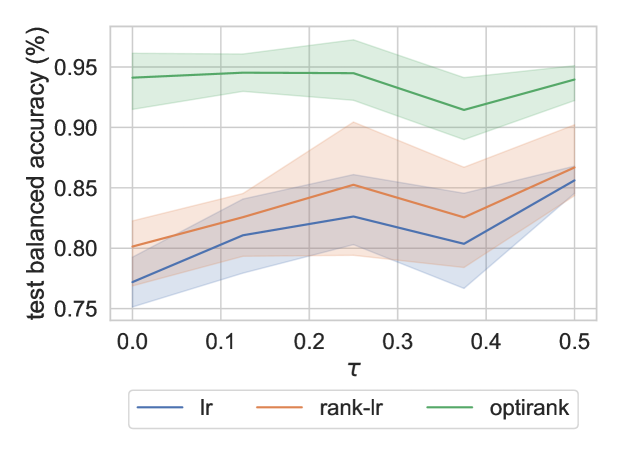
Figure 3: Dependence of test-accuracy with respect to the simulation parameter $\tau$. Default simulation parameters were set to $d=50$, $d_{P}=40$, $n=1000$, and $\sigma=0.05$.

D.3.2 Overlap between the true $\gamma$ and the one fitted by optirank

Appendix E Results on real data

E.1 Datasets

In this section we detail the data sources and the selection of examples used for each of the classification tasks.

TCGA.

The public count-table for the RNA-Seq data (with dbGab accession number phs000178.v10.p8) and the metadata was downloaded from the GDC data portal (https://portal.gdc.cancer.gov). We selected primary tumors with RNA-Seq data, with disease type in (’Adenomas and Adenocarcinomas’, ’Squamous Cell Neoplasms’, ’Cystic, Mucinous and Serous Neoplasms’, ’Ductal and Lobular Neoplasms’) and tissue of primary in (’Breast’,’Bronchus and lung’,’Esophagus’,’Stomach’,’Colon’,’Stomach’,’Pancreas’,’Rectum’, ’Rectosigmoid junction’, ’Prostate’). The label for the classification task was taken from the tissue of primary, by agglomerating "Colon", "Rectum" and "Rectosigmoid junction" in one class called "Colorectal".

Note.

In the task TCGA-PCAWG-met500, we ensured the binary problems One-vs-Rest involved a positive class present in the auxiliary source dataset PCAWG. For this reason, we had to remove the binary problems "Bronchus and lung" VS Rest and "Prostate" VS Rest.

PCAWG.

The PCAWG dataset comprises among other the TCGA dataset. Care was taken to exclude instances from the PCAWG that belong to the TCGA dataset during the selection of examples. The RNA-Seq data was downloaded from https://dcc.icgc.org/releases/PCAWG/transcriptome/transcript_expression and the metadata from https://dcc.icgc.org/releases/PCAWG/transcriptome/metadata. The same disease types and tissues of primary as in TCGA were selected, the class labels were processed in the same way.

BRCA.

The mutation status of the BRCA1 and BRCA2 genes for the examples selected in the TCGA was obtained on the GDC data portal, and aggregated into one binary class label indicating the presence of at least one mutation among BRCA1 and BRCA2. We selected instances whose tissue of primary was the Breast. The expression data is the same as the one in the TCGA.

met-500.

The expression data and the metadata was downloaded from https://xenabrowser.net/datapages/?cohort=MET500%20(expression%20centric). Only metastatic tumors were selected, of the same primary tissue as in the TCGA. The class-label was generated with the tissue of primary.

Single-Cell datasets: Baron, Murano, Segerstolpe, MWS, TM10x, TMfacs

The datasets were downloaded from https://github.com/pcahan1/singleCellNet#trainsets. For each task consisting of a pair/triplet of datasets, only common genes and common cell types were selected. Here is a short description per dataset:

Murano. Adult human pancreatic cells, sequenced with CEL-Seq2 (2120 cells)

Baron. Adult human pancreatic cells, sequenced with inDrop (8596 cells)

Segerstolpe. Adult human pancreatic cells, sequenced with Smart-Seq2 (2209 cells)

MWS. Adult mouse cells, across 125 cell types, sequenced with Microwell-seq (6477 cells)

TM10x. Adult mouse cells, across 32 cell types, sequenced by 10x (1599 cells)

TMfacs. Adult mouse cells across 69 cell types, sequenced by smartseq2 (3182 cells)

E.2 Pre-processing

All datasets were pre-processed with the pre-processing pipeline of SingleCellNet, detailed in Appendix C.1.1.

E.3 Cross-validation splits

In this appendix, we detail, per experiment and for each classification task, which dataset(s) and which training-testing scheme were used. All splits were realized in a stratified fashion.

E.3.1 Cross-validation splits for the tasks of section 6.1.

TCGA.

10% of the TCGA dataset was held out as a test set. The remaining 90% was used for 5-fold internal cross-validation.

PCAWG.

The same training set and cross-validation splits as in TCGA were used. The PCAWG dataset was used as a test set.

met-500.

The same training set and cross-validation splits as in TCGA were used. The met-500 dataset was used as a test set.

BRCA.

The dataset was split in four equal parts (each containing the same percentage of BRCA1 and BRCA2 mutated instances). A nested-cross validation scheme was applied in which for every possible combination, 2 parts are used for training, the third for validation, and the fourth for testing.

Cell-typing single-cell data.

For each task called X-Y (for instance Baron-Murano), dataset X was used as a training set and dataset Y as a test set. The training data was generated by randomly picking (maximum) 100 cells for each cell type. The rest of the training data is used for validation. This process is done 5 times. The test dataset is used as a whole.

E.3.2 Cross-validation splits for the tasks of section 6.2 in the multi-source and single-source scenario

We now describe the cross-validation splits in the tasks involving three datasets: one main source dataset, a auxiliary source dataset and a target dataset. These tasks are named with the pattern X-Y-Z, where X is the main source dataset, Y the auxiliary source dataset and Z the target dataset (for instance TCGA-PCAWG-met500). we distinguish two training scenarios: the multi-source and single-source scenarios. In the multi-source scenario, datasets X and Y are merged, both in the train and validation splits.
In the single-source scenario dataset Y is not used (except by ANrank-lr which uses dataset Y in its entirety, for the sole purpose of selecting the reference genes during the training phase). Indeed, in the single-source scenario, ANrank-lr does not use dataset Y for fitting the coefficients of the logistic regression nor for validation.

TCGA-PCAWG-met500.

We used 5-fold cross-validation to divide the TCGA and PCAWG datasets into train/validation splits, for each dataset separately. In the single-source scenario, only the TCGA is used. In the multi-source scenario, we compose each train and validation split by doing the union of the corresponding splits in the TCGA and PCAWG cross-validation splits.

Cell-typing single-cell data.

In the single-source setting, we pick randomly from dataset X 100 cells for each cell-type, the rest of dataset X goes in the validation split. We repeat this 5 times to generate 5 validation folds. ANrank-lr  uses a small(er) version of dataset Y, which comprise 100 cells for each cell-type.
In the multi-source scenario, we took care not to augment the size of the training set. To achieve this, we used the same CV splits as in the single-source setting, except that we downsampled to 50 the number of examples from dataset X for each cell-type, to which we added 50 examples of dataset Y for each cell-type. We added to the validation splits generated in the single-source setting the portion of dataset Y which was not used in the training set.

E.4 Hyperparameter grid

In table 5, we list the hyperparameters tuned for each classifier, and the corresponding values which were tried in the parameter grid.

Classifier	Parameter Name	Values
optirank	$\lambda_{1}$	{0, 0.0001, 0.001, 0.01, 0.1}
	$\lambda_{2}$	{0, 0.0001, 0.001, 0.01, 0.1}
	$\nicefrac{{s}}{{d}}$	{0.005, 0.01, 0.02, 0.05, 0.1, 0.2, 0.4, 0.6, 0.8, 1.0}
ANrank-lr	$\lambda_{1}$	{0, 0.0001, 0.001, 0.01, 0.1}
	$\lambda_{2}$	{0, 0.0001, 0.001, 0.01, 0.1}
	$\nicefrac{{s}}{{d}}$	{0.005, 0.01, 0.02, 0.05, 0.1, 0.2, 0.4, 0.6, 0.8, 1.0}
lr	$\lambda_{1}$	{0, 0.0001, 0.001, 0.01, 0.1)
	$\lambda_{2}$	{0, 0.0001, 0.001, 0.01, 0.1}
rank-lr	$\lambda_{1}$	{0, 0.0001, 0.001, 0.01, 0.1}
	$\lambda_{2}$	{0, 0.0001, 0.001, 0.01, 0.1}
rf	-	-
SCN	-	-

Table 5: Hyperparameters for classifiers in Section 6.1.4. Note that the dimension $d$ is 1000 for all classifiers.

Note that in the scikit-learn implementation of the logistic regression, the elastic net regularization is prescribed by the parameters $C$ and $\ell_{1}$_ratio. Therefore, these parameters were set according to the values of $\lambda_{1}$ and $\lambda_{2}$.

E.5 Comparison between classifiers

Scoring function: Balanced Accuracy.

The balanced accuracy scoring function was used as a a scoring metric both for hyperparameter selection and for model evaluation.
The balanced accuracy equals the average of sensitivity (true positive rate) and specificity (true negative rate), and is defined as such:

$$\text{balanced accuracy}=\nicefrac{{1}}{{2}}\left(\cfrac{TP}{TP+FN}+\cfrac{TN}{TN+FP}\right),$$ (37)

where TP stands for the number of true positives, FN for the false negatives, etc..

Note that in a balanced setting, the above formula reduces to the conventional accuracy. By contrast, in an unbalanced setting, a classifier which predicts all the time the predominant class will achieve a score of $\nicefrac{{1}}{{2}}$.

E.5.1 Hyperparameter selection and model evaluation

In this subsection, we describe how hyperparameters were chosen and how the resulting model was evaluated and compared to its competitors.

Each multi-class classification task was separated in $n_{classes}$ One-VS-Rest binary classification tasks, the binary classification tasks were left as is. Each classifier was trained for each parameter combination, in each binary problem, for each (internal) training split, and tested in the corresponding validation set and on the test set. In each binary task, for every test set (there is a unique one apart in the task BRCA), we selected the hyperparameters with the one-standard-error rule applied to the balanced accuracy averaged over validation splits. More precisely, we selected the sparsest model whose averaged balanced accuracy was within one standard error of the highest averaged balanced accuracy. We did not refit each classifier with the optimal hyper-parameter combination on the whole training set. Instead, for computational reasons, we kept as many models as the number of validation splits, and, as a result, the test-score, as displayed in table 3, was calculated with the average test score among those classifiers.

E.5.2 Pairwise comparisons

The following section details how each pair of classifier was compared, in order to determine if one performs significantly better than the other. In order to do so, we performed the comparison per dataset. We computed the difference in balanced accuracy between the two classifiers for each validation fold and each binary classification task (in such a way that no average is involved). Every one of those differences was accumulated as an independent observation, and a paired Student’s t-test was used to determine, based on the differences, if one classifier outperformed the other on the dataset at hand. (We used a two-sided test with a significance level of 5 %).

Table 6 through 19 show the result of the pairwise comparisons in each task. On the lower left part of each table, the sign at position (i,j) indicates if the classifier corresponding to row i is significantly better (+) or worse (-) than the classifier in column j. The percentages in the upper-right part indicate the fraction of instances where classifier i performed better than classifier j. In addition, whenever this percentage is associated with the algorithm on line i significantly outperforming the algorithm in column j the number is highlighted in bold green, and conversely, if this number correspond to a case where the algorithm on row i performs significantly worse then algorithm in column j, it is highlighted in red italic.

E.5.3 Pairwise comparisons for the classification tasks of section 6.1

Table 6: Pairwise comparisons for the task BRCA

	optirank	SCN	rank-lr	lr	rf
optirank		$50$	$83$	67	$50$
SCN			75	92	$58$
rank-lr		+		$75$	17
lr	+	+			8
rf			-	-

Table 7: Pairwise comparisons for the task TCGA

	optirank	SCN	rank-lr	lr	rf
optirank		0	$40$	$44$	0
SCN	-		96	96	72
rank-lr		+		$24$	0
lr		+			0
rf	-	+	-	-

Table 8: Pairwise comparisons for the task PCAWG

	optirank	SCN	rank-lr	lr	rf
optirank		$44$	$40$	$32$	20
SCN			$52$	$40$	0
rank-lr				$36$	20
lr					16
rf	-	-	-	-

Table 9: Pairwise comparisons for the task met-500

	optirank	SCN	rank-lr	lr	rf
optirank		24	$40$	36	24
SCN	-		72	56	12
rank-lr		+		$24$	4
lr	-	+			20
rf	-	-	-	-

Table 10: Pairwise comparisons for the task Baron-Murano

	optirank	SCN	rank-lr	lr	rf
optirank		15	$62$	18	25
SCN	-		85	$62$	25
rank-lr		+		12	25
lr	-		-		22
rf	-	-	-	-

Table 11: Pairwise comparisons for the task Baron-Segerstolpe

	optirank	SCN	rank-lr	lr	rf
optirank		$29$	$49$	$24$	0
SCN			$62$	$58$	7
rank-lr				$27$	2
lr					0
rf	-	-	-	-

Table 12: Pairwise comparisons for the task MWS-TM10x

	optirank	SCN	rank-lr	lr	rf
optirank		19	$49$	$60$	7
SCN	-		76	84	7
rank-lr		+		$56$	7
lr		+			0
rf	-	-	-	-

Table 13: Pairwise comparisons for the task MWS-TMfacs

	optirank	SCN	rank-lr	lr	rf
optirank		14	$39$	$32$	8
SCN	-		84	88	7
rank-lr		+		$33$	6
lr		+			5
rf	-	-	-	-

Table 14: Pairwise comparisons for the task TM10x-MWS

	optirank	SCN	rank-lr	lr	rf
optirank		20	47	77	16
SCN	-		81	86	30
rank-lr	-	+		70	13
lr	+	+	+		14
rf	-	-	-	-

Table 15: Pairwise comparisons for the task TM10x-TMfacs

	optirank	SCN	rank-lr	lr	rf
optirank		7	$53$	50	4
SCN	-		96	89	10
rank-lr		+		45	1
lr	-	+	-		7
rf	-	-	-	-

Table 16: Pairwise comparisons for the task TMfacs-MWS

	optirank	SCN	rank-lr	lr	rf
optirank		18	55	78	19
SCN	-		80	88	29
rank-lr	+	+		71	11
lr	+	+	+		12
rf	-	-	-	-

E.5.4 Pairwise comparisons for the classification tasks of section 6.2, in the single-source scenario

Table 17: Pairwise comparisons for the task Baron-Segerstolpe-Murano

	optirank	ANrank-lr	SCN	rank-lr	lr	rf
optirank		$28$	12	$50$	15	22
ANrank-lr			38	$78$	50	25
SCN	-	-		90	$60$	25
rank-lr			+		2	22
lr	-	-		-		20
rf	-	-	-	-	-

Table 18: Pairwise comparisons for the task MWS-TMfacs-TM10x

	optirank	ANrank-lr	SCN	rank-lr	lr	rf
optirank		$33$	20	32	$47$	8
ANrank-lr			32	$63$	$53$	8
SCN	-	-		73	72	8
rank-lr	-		+		$50$	8
lr			+			10
rf	-	-	-	-	-

Table 19: Pairwise comparisons for the task TCGA-PCAWG-met500

	optirank	ANrank-lr	SCN	rank-lr	lr	rf
optirank		$52$	12	$40$	24	12
ANrank-lr			4	$12$	8	8
SCN	-	-		72	68	16
rank-lr			+		$32$	12
lr	-	-	+			16
rf	-	-	-	-	-

E.5.5 Pairwise comparisons for the classification tasks of section 6.2, in the multi-source scenario

Table 20: Pairwise comparisons for the task Baron-Segerstolpe-Murano

	optirank	ANrank-lr	SCN	rank-lr	lr	rf
optirank		$28$	0	$45$	10	10
ANrank-lr			5	62	38	10
SCN	-	-		98	78	20
rank-lr		+	+		22	12
lr	-	-	+	-		12
rf	-	-	-	-	-

Table 21: Pairwise comparisons for the task MWS-TMfacs-TM10x

	optirank	ANrank-lr	SCN	rank-lr	lr	rf
optirank		$43$	18	$55$	22	5
ANrank-lr			15	$58$	27	7
SCN	-	-		83	85	15
rank-lr			+		20	3
lr	-	-	+	-		8
rf	-	-	-	-	-

Table 22: Pairwise comparisons for the task TCGA-PCAWG-met500

	optirank	ANrank-lr	SCN	rank-lr	lr	rf
optirank		68	$36$	56	80	48
ANrank-lr	+		20	36	$28$	12
SCN		-		$56$	56	$16$
rank-lr	+	-			56	20
lr	+		+	+		20
rf	-	-		-	-

E.5.6 Comparisons in terms of sparsity

In Section 6.1.4, we highlighted the fact that optirank, compared to rank-lr has the added beneficial potential to produce sparse solutions. In fact, by definition, rank-lr necessitates to know the value of all genes to perform the ranking.
However, it was mentioned that on instances where lr performed well, there was no advantage in using optirank, as the solutions of lr are usually sparser than the ones produced by optirank. In the following, we support this claim.

As a first investigation, we computed per dataset the average number of genes of the solution found by optirank and lr. Note that for optirank, the effective number of genes is the number of genes which are either in the reference set indicated by $\boldsymbol{\gamma}$ or whose corresponding coefficient $w_{j}$ is non-zero. Table 23 summarizes the results and it is clear that lr produces sparser solutions than optirank.

	$\overline{s_{\text{{or}}}}$	$\overline{s_{\text{{lr}}}}$	$100\,\hat{P}(s_{\text{{or}}}\!\leq\!s_{\text{{lr}}})$	$100\,\hat{P}(s_{\text{{lr}}}\!\leq\!s_{\text{{or}}})$
BRCA	454	43	8	92
TCGA	598	588	24	76
PCAWG	598	588	24	76
met-500	598	588	24	76
Baron-Murano	462	406	57	42
Baron-Segerstolpe	511	451	44	67
MWS-TM10x	629	365	21	79
MWS-TMfacs	666	226	9	91
TM10x-MWS	514	242	27	73
TM10x-TMfacs	616	305	36	64
TMfacs-MWS	530	204	25	75

Table 23: Number of genes $s_{\text{{or}}}$ and $s_{\text{{lr}}}$ in the solutions produced by optirank and lr  (2 outermost left columns), averaged across folds and classes. The third column shows the percentage $100\,\hat{P}(s_{\text{{or}}}\!\leq\!s_{\text{{lr}}})$ of instances where the solution of optirank is sparser than the solution found by lr. The last column shows the percentage $100\,\hat{P}(s_{\text{{lr}}}\!\leq\!s_{\text{{or}}})$ of instances with the opposite case, i.e where the solution of optirank is less sparse than the solution found by lr.

In fact, in the task BRCA, optirank rarely produces a sparser solution, and on other tasks, apart from the task Baron-Murano and TMfacs-MWS, lr produces sparser solutions in a majority of cases. It should be clear however that in all cases where some robustness can be obtained by using a rank representation, the classical rank representation requires to measure all genes and has thus no sparsity whatsoever, while optirank attempts by construction to use a reduced set of genes, and so, even if the level of sparsity obtained is not comparable to that of an lr model the gain in performance might be worth it.

E.5.7 Comparisons in terms of sparsity in the multi-source scenario

We carried the same analysis than in the previous section for the tasks in the multi-source scenario (see Section 6.2). As in previous section, lr produces sparser solutions than optirank and ANrank-lr in a majority of cases. It is worth noting that solutions found by ANrank-lr and optirank require a similar number of genes, with optirank producing slightly sparser solutions.

	$\overline{s_{\text{{or}}}}$	$\overline{s_{\text{{Ar}}}}$	$\overline{s_{\text{{lr}}}}$	$100\,\hat{P}(s_{\text{{or}}}\!\leq\!s_{\text{{others}}})$	$100\,\hat{P}(s_{\text{{Ar}}}\!\leq\!s_{\text{{others}}})$	$100\,\hat{P}(s_{\text{{lr}}}\!\leq\!s_{\text{{others}}})$
TCGA-PCAWG-met500	844	849	273	20	0	80
Baron-Segerstolpe-Murano	606	658	364	12	12	75
MWS-TMfacs-TM10x	604	796	300	15	2	83

Table 24: Number of genes $s_{\text{{or}}}$, $s_{\text{{Ar}}}$, and $s_{\text{{lr}}}$ in the solutions produced by optirank, ANrank-lr and lr (3 outermost left columns), averaged across folds and classes. The last three columns shows the percentage of instances where the solution of the indicated classifier is sparser than the ones found by the other classifiers.

E.5.8 Supplementary table for single-source scenario

	ANrank-lr	SCN	lr	optirank	rank-lr	rf
TCGA-PCAWG-met500	$\mathbf{80\pm 3}$ (2)	$66\pm 4$ (5)	$74\pm 4$ (4)	$\mathbf{81\pm 4}$ (1)	$\mathbf{76\pm 3}$ (3)	$61\pm 4$ (6)
Baron-Segerstolpe-Murano	$\mathbf{93\pm 1}$ (3)	$89.4\pm 1.5$ (5)	$89.5\pm 2.4$ (4)	$\mathbf{93.7\pm 1.5}$ (2)	$\mathbf{93.8\pm 1.7}$ (1)	$62\pm 3$ (6)
MWS-TMfacs-TM10x	$\mathbf{82\pm 2}$ (4)	$72\pm 2$ (5)	$\mathbf{83.3\pm 2.2}$ (2)	$\mathbf{84\pm 2}$ (1)	$83.0\pm 2.4$ (3)	$53\pm 1$ (6)

Table 25: Single-source scenario. Average balanced accuracies in % (across folds and classes) of competing classifiers on the tasks detailed in section 6.2 in the case in which the auxiliary source dataset is not used (except for ANrank-lr  which uses it for ranking reference genes selection). The integer in parenthesis denotes the rank of the classifiers in terms of average balanced accuracy (lower is better). Classifiers which did not score significantly worse than the best classifier according to a paired Student’s t-test (with a 5% significance level) are highlighted in bold (see Appendix E.5 for additional details).

E.5.9 Runtime comparisons

Table 26 shows the average runtime (in seconds) across validation splits and binary problems of competing classifiers with the hyperparameters set to their optimal values according to the one-standard-error-rule. We applied our comparison on the tasks detailed in 6.2, with classifiers trained in the single-source scenario. The results attest that the fitting time of optirank  is reasonable, and on some tasks, it is even lower than the fitting time of its competitors using rank features such as ANrank-lr and rank-lr.

	ANrank-lr	SCN	lr	optirank	rank-lr	rf
TCGA-PCAWG-met500	135 ± 38	205.6 ± 0.8	140 ± 47	70 ± 4	150 ± 46	8.6 ± 0.5
Baron-Segerstolpe-Murano	10 ± 1	50.8 ± 0.1	2.0 ± 0.3	7.7 ± 0.7	3.6 ± 0.3	0.75 ± 0.01
MWS-TMfacs-TM10x	8.8 ± 0.5	33.82 ± 0.09	2.5 ± 0.2	16 ± 2	36 ± 9	0.92 ± 0.02

Table 26: Runtime estimates. Average runtime (in seconds) across validation splits and binary problems of competing classifiers for the hyperparameter set which was selected as optimal according to the one-standard-error-rule. All classifiers were trained in the single-source scenario.

Appendix F Computational resources

The computational results in this work were produced with an internal computing cluster, in a batched fashion, amounting to a total of 2500 CPU hours. Per batch, the maximal capacity used was 30 GB of RAM with 2 CPUs.

References

- Amerise and Tarsitano, (2015) Amerise, I. L. and Tarsitano, A. (2015). Correction methods for ties in rank correlations. Journal of Applied Statistics, 42(12):2584–2596.
- Cascianelli et al., (2020) Cascianelli, S., Molineris, I., Isella, C., Masseroli, M., and Medico, E. (2020). Machine learning for RNA sequencing-based intrinsic subtyping of breast cancer. Scientific Reports, 10:14071.
- Csiba and Richtárik, (2017) Csiba, D. and Richtárik, P. (2017). Global convergence of arbitrary-block gradient methods for generalized Polyak-Łojasiewicz functions. arXiv preprint arXiv:1709.03014.
- Defazio et al., (2014) Defazio, A., Bach, F., and Lacoste-Julien, S. (2014). SAGA: A fast incremental gradient method with support for non-strongly convex composite objectives.
- Dillies et al., (2012) Dillies, M.-A., Rau, A., Aubert, J., Hennequet-Antier, C., Jeanmougin, M., Servant, N., Keime, C., Marot, G., Castel, D., Estelle, J., Guernec, G., Jagla, B., Jouneau, L., Laloë, D., Gall, C., Schaëffer, B., Le Crom, S., Guedj, M., and Jaffrézic, F. (2012). A comprehensive evaluation of normalization methods for illumina high-throughput RNA sequencing data analysis. Briefings in bioinformatics, 14.
- Duchi et al., (2008) Duchi, J., Shalev-Shwartz, S., Singer, Y., and Chandra, T. (2008). Efficient projections onto the l1-ball for learning in high dimensions. In ICML ’08: Proceedings of the 25th international conference on Machine learning, pages 272–279.
- Evans et al., (2016) Evans, C., Hardin, J., and Stoebel, D. (2016). Selecting between-sample RNA-seq normalization methods from the perspective of their assumptions. Briefings in bioinformatics, 19.
- Hastie et al., (2015) Hastie, T., Tibshirani, R., and Wainwright, M. (2015). Statistical Learning with Sparsity: The Lasso and Generalizations. Chapman and Hall/CRC.
- Kendall, (1945) Kendall, M. G. (1945). The treatment of ties in ranking problems. Biometrika, 33(3):239–251.
- Laprovitera et al., (2021) Laprovitera, N., Riefolo, M., Ambrosini, E., Klec, C., Pichler, M., and Ferracin, M. (2021). Cancer of unknown primary: Challenges and progress in clinical management. Cancers, 13:451.
- Lausser et al., (2016) Lausser, L., Schmid, F., Schirra, L.-R., Wilhelm, A., and Kestler, H. (2016). Rank-based classifiers for extremely high-dimensional gene expression data. Advances in Data Analysis and Classification, 12:1–20.
- Leek et al., (2010) Leek, J. T., Scharpf, R. B., Bravo, H. C., Simcha, D., Langmead, B., Johnson, W. E., Geman, D., Baggerly, K., and Irizarry, R. A. (2010). Tackling the widespread and critical impact of batch effects in high-throughput data. Nature Reviews Genetics, 11(10):733–739.
- Leiserson et al., (2015) Leiserson, M. D. M., Gramazio, C. C., Hu, J., Wu, H.-T., Laidlaw, D. H., and Raphael, B. J. (2015). MAGI: visualization and collaborative annotation of genomic aberrations. Nature Methods, 12(6):483–484.
- Pedregosa et al., (2011) Pedregosa, F., Varoquaux, G., Gramfort, A., Michel, V., Thirion, B., Grisel, O., Blondel, M., Prettenhofer, P., Weiss, R., Dubourg, V., Vanderplas, J., Passos, A., Cournapeau, D., Brucher, M., Perrot, M., and Duchesnay, E. (2011). Scikit-learn: Machine learning in Python. Journal of Machine Learning Research, 12:2825–2830.
- Razaviyayn et al., (2013) Razaviyayn, M., Hong, M., and Luo, Z.-Q. (2013). A unified convergence analysis of block successive minimization methods for nonsmooth optimization. SIAM Journal on Optimization, 23(2):1126–1153.
- Scialdone et al., (2015) Scialdone, A., Natarajan, K. N., Saraiva, L. R., Proserpio, V., Teichmann, S. A., Stegle, O., Marioni, J. C., and Buettner, F. (2015). Computational assignment of cell-cycle stage from single-cell transcriptome data. Methods, 85:54–61.
- Shen et al., (2020) Shen, Y., Chu, Q., Yin, X., He, Y., Bai, P., Wang, Y., Fang, W., Timko, M., Fan, L., and Jiang, W. (2020). Tod-cup: a gene expression rank-based majority vote algorithm for tissue origin diagnosis of cancers of unknown primary. Briefings in bioinformatics, 22.
- Shi et al., (2014) Shi, J. V., Xu, Y., and Baraniuk, R. G. (2014). Sparse bilinear logistic regression. arXiv preprint arXiv:1404.4104.
- Sun et al., (2015) Sun, S., Shi, H., and Wu, Y. (2015). A survey of multi-source domain adaptation. Information Fusion, 24:84–92.
- Tan and Cahan, (2019) Tan, Y. and Cahan, P. (2019). SingleCellNet: A computational tool to classify single cell RNA-seq data across platforms and across species. Cell Systems, 9(2):207–213.e2.
- The Cancer Genome Atlas Research Network et al., (2008) The Cancer Genome Atlas Research Network et al. (2008). Comprehensive genomic characterization defines human glioblastoma genes and core pathways. Nature, 455(7216):1061–1068.
- The ICGC/TCGA Pan-Cancer Analysis of Whole Genomes Consortium, (2020) The ICGC/TCGA Pan-Cancer Analysis of Whole Genomes Consortium (2020). Pan-cancer analysis of whole genomes. Nature, 578(7793):82–93.
- Tseng and Yun, (2009) Tseng, P. and Yun, S. (2009). A coordinate gradient descent method for nonsmooth separable minimization. Mathematical Programming, 117(1):387–423.
- Xu and Yin, (2013) Xu, Y. and Yin, W. (2013). A block coordinate descent method for regularized multiconvex optimization with applications to nonnegative tensor factorization and completion. SIAM Journal on imaging sciences, 6(3):1758–1789.
- Zaslavskiy et al., (2009) Zaslavskiy, M., Bach, F., and Vert, J.-P. (2009). A path following algorithm for the graph matching problem. IEEE Transactions on Pattern Analysis and Machine Intelligence, 31(12):2227–2242.
- Zou and Hastie, (2005) Zou, H. and Hastie, T. (2005). Regularization and variable selection via the elastic net. Journal of the Royal Statistical Society: Series B (Statistical Methodology), 67(2):301–320.