Multivariate Regression via Enhanced Response Envelope: Envelope Regularization and Double Descent

Abstract

The envelope model provides substantial efficiency gains over the standard multivariate linear regression by identifying the material part of the response to the model and by excluding the immaterial part. In this paper, we propose the enhanced response envelope by incorporating a novel envelope regularization term in its formulation. It is shown that the enhanced response envelope can yield better prediction risk than the original envelope estimator. The enhanced response envelope naturally handles high-dimensional data for which the original response envelope is not serviceable without necessary remedies. In an asymptotic high-dimensional regime where the ratio of the number of predictors over the number of samples converges to a non-zero constant, we characterize the risk function and reveal an interesting double descent phenomenon for the first time for the envelope model. A simulation study confirms our main theoretical findings. Simulations and real data applications demonstrate that the enhanced response envelope does have significantly improved prediction performance over the original envelope method.

Keywords: Double descent, Envelope model, High-dimension asymptotics, Prediction, Regularization

1 Introduction

The envelope model first introduced by Cook et al. (2010) is a modern approach to estimating an unknown regression coefficient matrix $\bm{\beta}\in\mathbb{R}^{r\times p}$ in multivariate linear regression of the response vector $\mathbf{y}\in\mathbb{R}^{r}$ on the predictors $\mathbf{x}\in\mathbb{R}^{p}$. It was shown by Cook et al. (2010) that the envelope estimator of $\bm{\beta}$ results in substantial efficiency gains relative to the standard maximum likelihood estimator of $\bm{\beta}$. The gains arise by identifying the part of the response vector that is material to the regression and by excluding the immaterial part in the estimation. The original envelope model has been later extended to the envelope model based on excluding immaterial parts of the predictors to the regression by Cook et al. (2013). Cook et al. (2013) then established the connection between the latter envelope model and partial least squares, providing a statistical understanding of partial least squares algorithms.

The success of the envelope models and their theories motivated some authors to propose new envelope models by applying or extending the core idea of envelope modeling to various statistical models. The two most common are the response envelope models and the predictor envelope models. The response envelope models (predictor envelope models) achieve estimation and prediction gains by eliminating the variability arising from the immaterial part of the responses (predictors) that is invariant to the changes in the predictors (responses). Papers on response envelope models include the original envelope model (Cook et al., 2010), the partial envelope model (Su and Cook, 2011), the scaled response envelope model (Cook and Su, 2013), the reduced-rank envelope model (Cook et al., 2015), the sparse envelope model (Su et al., 2016), the Bayesian envelope model (Khare et al., 2017), the tensor response envelope model (Li and Zhang, 2017), the envelope model for matrix variate regression (Ding and Cook, 2018), and the spatial envelope model for spatially correlated data (Rekabdarkolaee et al., 2020). Papers on predictor envelope models include the envelope model for predictor reduction (Cook et al., 2013), the envelope model for generalized linear models and Cox’s proportional hazard model (Cook and Zhang, 2015a), the scaled predictor envelope model (Cook and Su, 2016), the envelope quantile regression model (Ding et al., 2020), the envelope model for the censored quantile regression (Zhao et al., 2022), tensor envelope partial least squares regression (Zhang and Li, 2017), and envelope-based sparse partial least squares regression (Zhu and Su, 2020). For a comprehensive review of the envelope models, readers are referred to Cook (2018).

High-dimensional data have become common in many fields. It is only natural to consider the performance of the envelope model under high dimensions. The likelihood-based method to estimate $\bm{\beta}$ under both the response/predictor envelope model is not serviceable for high-dimensional data because the likelihood-based method requires the inversion of the sample covariance matrix of predictors. Hence, one has to find effective ways to mitigate this issue. For the predictor envelope model, its connection to partial least squares provides one solution. Partial least squares (De Jong, 1993) can be used for estimating $\bm{\beta}$ for the predictor envelope model (Cook et al., 2013). The partial least squares algorithm is an iterative moment-based algorithm involving the sample covariance of predictors and the sample covariance between the response vector and predictors, which does not require inversion of the sample covariance matrix of predictors. In addition, the algorithm provides the root-$n$ consistent estimator of $\bm{\beta}$ in the predictor envelope model with the number of predictors fixed (Chun and Keleş, 2010; Cook et al., 2013) and can yield accurate prediction in the asymptotic high-dimensional regime when the response is univariate (Cook and Forzani, 2019). Motivated by this, Zhu and Su (2020) introduced envelope-based sparse partial least squares and showed the consistency of the estimator for the sparse predictor envelope model. Zhang and Li (2017) proposed a tensor envelope partial least squares algorithm, which provides the consistent estimator for the tensor predictor envelope model. Another way to apply predictor envelope models for high-dimensional data is by selecting the principal components of predictors and then using likelihood-based estimation on the principal components. This simple remedy is adapted by Rimal et al. (2019) to compare the prediction performance of the likelihood-based predictor envelope method, principal component regression, and partial least squares regression for high-dimensional data. Their extensive numerical study showed that this simple remedy produced better prediction performance than principal component regression and partial least squares regression. The impact of high dimensions is more severe for the response envelope. There is far less work on making the response envelope model serviceable for high-dimensional data. The Bayesian approach for the response envelope model (Khare et al., 2017) can handle high-dimensional data. The sparse envelope model (Su et al., 2016) which performs variable selection on the responses can handle data with the sample size smaller than the number of responses, but still requires the number of predictors smaller than the number of sample size.

In this paper, we propose the enhanced response envelope for high-dimensional data by incorporating a novel envelope regularization term in its formulation. The envelope regularization term respects the fundamental idea of the original envelope model by considering the presence of the material and immaterial parts of the response in the model. The enhancements are twofold. First, our enhanced response envelope estimator can handle both low- and high-dimensional data, while the original envelope estimator can only handle low-dimensional data where the sample size $n$ is smaller than the number of predictors $p$. From the connection between the original envelope estimator and the enhanced response envelope estimator in low-dimension, we extend the definition of the original envelope estimator to high-dimensional data by considering the limiting case of the enhanced response envelope estimator with a vanishing regularization parameter; see the discussion in Section 2.3. Second, we prove that the enhanced response envelope can reduce the prediction risk relative to the original envelope for all values of $n$ and $p$. Moreover, we study the asymptotics of the prediction risk for the original envelope estimator and the enhanced response envelope estimator when both $n,p\rightarrow\infty$ and their ratio converges to a nonzero constant $p/n\rightarrow\gamma\in(0,\infty)$. This kind of asymptotic regime has been considered in high-dimensional machine learning theory (El Karoui, 2018; Dobriban and Wager, 2018; Liang and Rakhlin, 2020; Hastie et al., 2022) for analyzing the behavior of prediction risk of certain predictive models. We derive an interesting asymptotic prediction risk curve for the envelope estimator. The risk increases as $\gamma$ increases, and then decreases after $\gamma>1$. This phenomenon is known as the double descent phenomenon in the machine learning literature. Although the double descent phenomenon has been observed for neural networks and ridgeless regression (Belkin et al., 2019; Hastie et al., 2022), this is the first time that such a phenomenon is shown for the envelope models.

The rest of the paper is organized as follows. We review the original envelope model and the corresponding envelope estimator in Section 2.1. In Section 2.2, we introduce a new regularization term called the envelope regularization based on which we propose the enhanced response envelope in section 2.3. The enhanced response envelope estimator naturally provides a definition for the envelope estimator when $p>n$. Section 2.4 describes how to implement this new method in practice. In Section 3.1, we prove that the enhanced response envelope can yield better prediction risk than the original envelope for any $(n,p)$ pair. Considering $n,p\rightarrow\infty$ and $p/n\rightarrow\gamma\in(0,\infty)$, we derive the limiting prediction risk result of the original envelope and the enhanced response envelope in Section 3.2. This result along with our simulation study in Section 4 verify the double descent phenomenon. Real data analyses are presented in Section 5. Proofs of theorems are provided in Appendix A.

2 Enhanced response envelope

2.1 Review of envelope model

Envelope model Let us begin with the classical multivariate linear regression model of a response vector $\mathbf{y}\in\mathbb{R}^{r}$ given a predictor vector $\mathbf{x}\in\mathbb{R}^{p}$:

$$\mathbf{y}=\bm{\beta}\mathbf{x}+\bm{\varepsilon},~{}\bm{\varepsilon}\sim N(\mathbf{0},\bm{\Sigma}),$$ (1)

where $\bm{\varepsilon}$ is the error vector with a positive definite $\bm{\Sigma}$ and independent to $\mathbf{x}$. $\bm{\beta}\in\mathbb{R}^{r\times p}$ is an unknown matrix of regression coefficients and $\mathbf{x}\sim P_{\mathbf{x}}$ where $P_{\mathbf{x}}$ is a distribution on $\mathbb{R}^{p}$ such that $\mathrm{E}(\mathbf{x})=\mathbf{0}$ and $\mathrm{Cov}(\mathbf{x})=\bm{\Sigma}_{\mathbf{x}}$. We omit an intercept by assuming $\mathrm{E}(\mathbf{y})=\mathbf{0}$ for easy communication.

The envelope model allows for the possibility that there is a part of the response vector that is unaffected by changes in the predictor vector. Specifically, let $\mathcal{E}\subseteq\mathbb{R}^{r}$ be a subspace such that for all $\mathbf{x}_{1}$ and $\mathbf{x}_{2}$,

$$\text{(i)~{}}\mathbf{Q}_{\mathcal{E}}\mathbf{y}|(\mathbf{x}=\mathbf{x}_{1})\sim\mathbf{Q}_{\mathcal{E}}\mathbf{y}|(\mathbf{x}=\mathbf{x}_{2})~{}\text{ and }~{}\text{(ii)~{}}\mathbf{P}_{\mathcal{E}}\mathbf{y}\perp\!\!\!\perp\mathbf{Q}_{\mathcal{E}}\mathbf{y}|\mathbf{x},$$ (2)

where $\mathbf{P}_{\mathcal{E}}$ is the projection onto $\mathcal{E}$ and $\mathbf{Q}_{\mathcal{E}}=\mathbf{I}-\mathbf{P}_{\mathcal{E}}$. Condition (i) states that the marginal distribution of $\mathbf{Q}_{\mathcal{E}}\mathbf{y}$ is invariant to changes in $\mathbf{x}$. Condition (ii) says that $\mathbf{Q}_{\mathcal{E}}\mathbf{y}$ does not affect $\mathbf{P}_{\mathcal{E}}\mathbf{y}$ if $\mathbf{x}$ is provided. Conditions together imply that $\mathbf{P}_{\mathcal{E}}$ includes the relevant dependency information of $\mathbf{y}$ on $\mathbf{x}$ (the material part) while $\mathbf{Q}_{\mathcal{E}}$ is the irrelevant information (the immaterial part).

Let $\mathcal{B}=\text{span}(\bm{\beta})$. The conditions in (LABEL:eq:envlp-cond(1)) hold if and only if

$$\text{span}(\bm{\beta})=\mathcal{B}\subseteq\mathcal{E}~{}\text{ and }~{}\bm{\Sigma}=\mathbf{P}_{\mathcal{E}}\bm{\Sigma}\mathbf{P}_{\mathcal{E}}+\mathbf{Q}_{\mathcal{E}}\bm{\Sigma}\mathbf{Q}_{\mathcal{E}}.$$ (3)

The definition of an envelope introduced by Cook et al. (2007, 2010) formalizes the smallest subspace satisfying the conditions in (LABEL:eq:envlp-cond(1)) using the equivalence relation of (LABEL:eq:envlp-cond(1)) and (3). The envelope is defined as the intersection of all subspaces $\mathcal{E}$ satisfying (3) and is denoted by $\mathcal{E}_{\bm{\Sigma},\mathcal{B}}$, $\bm{\Sigma}$-envelope of $\mathcal{B}$.

The envelope model arises by parameterizing the multivariate linear model in terms of the envelope $\mathcal{E}_{\bm{\Sigma},\mathcal{B}}$. The parameterization is as follows. Let $u=\text{dim}(\mathcal{E}_{\bm{\Sigma},\mathcal{B}})$, $\bm{\Gamma}\in\mathbb{R}^{r\times u}$ be any semi-orthogonal basis matrix for $\mathcal{E}_{\bm{\Sigma},\mathcal{B}}$, and $\bm{\Gamma}_{0}\in\mathbb{R}^{r\times(r-u)}$ is any semi-orthogonal basis matrix for the orthogonal complement of $\mathcal{E}_{\bm{\Sigma},\mathcal{B}}$. Then the multivariate linear model can be written as

$$\mathbf{y}=\bm{\Gamma}\bm{\eta}\mathbf{x}+\bm{\varepsilon},~{}\bm{\varepsilon}\sim N(\mathbf{0},\bm{\Gamma}\bm{\Omega}\bm{\Gamma}^{T}+\bm{\Gamma}_{0}\bm{\Omega}_{0}\bm{\Gamma}_{0}^{T}),$$ (4)

where $\bm{\beta}=\bm{\Gamma}\bm{\eta}$ with $\bm{\eta}\in\mathbb{R}^{u\times p}$, and $\bm{\Omega}\in\mathbb{R}^{r\times r}$ and $\bm{\Omega}_{0}\in\mathbb{R}^{(r-u)\times(r-u)}$ are symmetric positive definite matrices. Model (4) is called the envelope model.

Envelope estimator The parameters in the envelope model are estimated by maximizing the likelihood function from model (4). Assume that $p{+}r<n$ and $u$ is the dimension $u$ of the envelope. $\mathbf{S}_{\mathbf{X}}=n^{-1}\mathbf{X}^{T}\mathbf{X}$, $\mathbf{S}_{\mathbf{Y}}=n^{-1}\mathbf{Y}^{T}\mathbf{Y}$, $\mathbf{S}_{\mathbf{Y},\mathbf{X}}=n^{-1}\mathbf{Y}^{T}\mathbf{X}$, and $\mathbf{S}_{\mathbf{Y}|\mathbf{X}}=\mathbf{S}_{\mathbf{Y}}-\mathbf{S}_{\mathbf{Y},\mathbf{X}}\mathbf{S}_{\mathbf{X}}^{-1}\mathbf{S}_{\mathbf{X},\mathbf{Y}}$, where $\mathbf{Y}\in\mathbb{R}^{n\times r}$ has rows $\mathbf{y}_{i}^{T}$ and $\mathbf{X}\in\mathbb{R}^{n\times p}$ has rows $\mathbf{x}_{i}^{T}$.

The envelope estimator of $\bm{\beta}$ is determined as

$$\hat{\mathcal{E}}_{\bm{\Sigma},\mathcal{B}}=\text{span}\{\arg\min_{\mathbf{G}\in\text{Gr}(r,u)}(\log|\mathbf{G}^{T}\mathbf{S}_{\mathbf{Y}|\mathbf{X}}\mathbf{G}|+\log|\mathbf{G}^{T}\mathbf{S}_{\mathbf{Y}}^{-1}\mathbf{G}|)\},$$ (5)

where $\text{Gr}(r,u)=\{\mathbf{G}\in\mathbb{R}^{r\times u}:\mathbf{G}\text{ is a semi-orthogonal matrix}\}$. Define $\hat{\bm{\Gamma}}$ as any semi-orthogonal basis matrix for $\hat{\mathcal{E}}_{\bm{\Sigma},\mathcal{B}}$ and let $\hat{\bm{\Gamma}}_{0}$ be any semi-orthogonal basis matrix for the orthogonal complement of $\hat{\mathcal{E}}_{\bm{\Sigma},\mathcal{B}}$. The estimator of $\bm{\beta}$ is given by

$$\hat{\bm{\beta}}=\hat{\bm{\Gamma}}\hat{\bm{\Gamma}}^{T}\mathbf{S}_{\mathbf{Y},\mathbf{X}}\mathbf{S}_{\mathbf{X}}^{-1},$$ (6)

and $\bm{\Sigma}$ is estimated by $\hat{\bm{\Sigma}}=\hat{\bm{\Gamma}}\hat{\bm{\Omega}}\hat{\bm{\Gamma}}+\hat{\bm{\Gamma}}_{0}^{T}\hat{\bm{\Omega}}_{0}\hat{\bm{\Gamma}}_{0}$ where

$$\hat{\bm{\Omega}}=\hat{\bm{\Gamma}}^{T}\mathbf{S}_{\mathbf{Y}|\mathbf{X}}\hat{\bm{\Gamma}},~{}~{}\hat{\bm{\Omega}}_{0}=\hat{\bm{\Gamma}}_{0}^{T}\mathbf{S}_{\mathbf{Y}}\hat{\bm{\Gamma}}_{0},$$ (7)

2.2 Envelope regularization

In this section, we introduce the envelope regularization term that respects the fundamental idea in the envelope model by considering the presence of material and immaterial parts, $\mathbf{P}_{\mathcal{E}_{\bm{\Sigma},\mathcal{B}}}\mathbf{y}$ and $\mathbf{Q}_{\mathcal{E}_{\bm{\Sigma},\mathcal{B}}}\mathbf{y}$, in the regression.

We define the envelope regularization term as

$$\rho(\bm{\eta},\bm{\Omega})=\text{tr}(\bm{\eta}^{T}\bm{\Omega}^{-1}\bm{\eta}).$$ (8)

The envelope model distinguishes between $\mathbf{P}_{\mathcal{E}_{\bm{\Sigma},\mathcal{B}}}\mathbf{y}$ and $\mathbf{Q}_{\mathcal{E}_{\bm{\Sigma},\mathcal{B}}}\mathbf{y}$ in the estimation process. The log-likelihood function of the envelope model is decomposed into two log-likelihood functions. One is the log-likelihood function for the multivariate regression of $\bm{\Gamma}^{T}\mathbf{y}$ on $\mathbf{x}$, $\bm{\Gamma}^{T}\mathbf{y}=\bm{\eta}\mathbf{x}+\bm{\Gamma}^{T}\bm{\varepsilon}$ where $\bm{\Gamma}^{T}\bm{\varepsilon}\sim N(\mathbf{0},\bm{\Omega})$. The other is the log-likelihood function for the zero-mean model of $\bm{\Gamma}_{0}^{T}\mathbf{y}$, $\bm{\Gamma}_{0}^{T}\mathbf{y}=\bm{\Gamma}_{0}^{T}\bm{\varepsilon}$ where $\bm{\Gamma}_{0}^{T}\bm{\varepsilon}\sim N(\mathbf{0},\bm{\Omega}_{0})$. The envelope regularization term (8) is the function of $\bm{\eta}$ and $\bm{\Omega}$, the parameters in the likelihood for the material part of the envelope model. The envelope regularization term (8) can be seen as imposing the Frobenius norm regularization on the coefficient after standardizing the material part of the regression to have uncorrelated errors, $\bm{\Omega}^{-1/2}\bm{\Gamma}^{T}\mathbf{y}=\bm{\Omega}^{-1/2}\bm{\eta}\mathbf{x}+\bm{\Omega}^{-1/2}\bm{\Gamma}^{T}\bm{\varepsilon}$ where $\bm{\Omega}^{-1/2}\bm{\Gamma}^{T}\bm{\varepsilon}\sim N(\mathbf{0},\mathbf{I})$.

We emphasize that the envelope regularization is different from the ridge regularization. While the ridge regularization $\|\bm{\beta}\|_{F}^{2}$ is the quadratic function of $\bm{\beta}$, the envelope regularization is not because the components of $\bm{\Omega}$ are not fixed values. The envelope regularization is the function of both $\bm{\eta}$ and $\bm{\Omega}$, and thus is optimized over $\bm{\eta}$ and $\bm{\Omega}$ simultaneously, as shown in the next subsection.

2.3 The proposed estimator

We only assume that $r\leq n$ but $p$ is allowed to be bigger than $n$. The log-likelihood function under the envelope model (4) is

$$\mathcal{L}_{u}(\bm{\eta},\mathcal{E}_{\bm{\Sigma},\mathcal{B}},\bm{\Omega},\bm{\Omega}_{0})= -(nr/2)\log(2\pi)-(n/2)\log|\bm{\Gamma}\bm{\Omega}\bm{\Gamma}^{T}+\bm{\Gamma}_{0}\bm{\Omega}_{0}\bm{\Gamma}_{0}^{T}|$$

$$-(1/2)\sum_{i=1}^{n}(\mathbf{y}_{i}-\bm{\Gamma}\bm{\eta}\mathbf{x}_{i})^{T}(\bm{\Gamma}\bm{\Omega}\bm{\Gamma}^{T}+\bm{\Gamma}_{0}\bm{\Omega}_{0}\bm{\Gamma}_{0}^{T})^{-1}(\mathbf{y}_{i}-\bm{\Gamma}\bm{\eta}\mathbf{x}_{i}).$$

By incorporating the envelope regularization term $\rho$ given in the last subsection, we propose the following enhanced response envelope estimator via penalized maximum likelihood:

$$\arg\max\{\mathcal{L}_{u}(\bm{\eta},\mathcal{E}_{\bm{\Sigma},\mathcal{B}},\bm{\Omega},\bm{\Omega}_{0})-\frac{n}{2}\lambda\cdot\rho(\bm{\eta},\bm{\Omega})\},$$ (9)

where $\lambda>0$ serves as a regularization parameter.

Let $\mathbf{S}_{\mathbf{X}}=n^{-1}\mathbf{X}^{T}\mathbf{X}$, $\mathbf{S}_{\mathbf{Y}}=n^{-1}\mathbf{Y}^{T}\mathbf{Y}$, $\mathbf{S}_{\mathbf{Y},\mathbf{X}}=n^{-1}\mathbf{Y}^{T}\mathbf{X}$, $\mathbf{S}^{\lambda}_{\mathbf{X}}=\mathbf{S}_{\mathbf{X}}+\lambda\mathbf{I}$ and $\mathbf{S}^{\lambda}_{\mathbf{Y}|\mathbf{X}}=\mathbf{S}_{\mathbf{Y}}-\mathbf{S}_{\mathbf{Y},\mathbf{X}}(\mathbf{S}_{\mathbf{X}}^{\lambda})^{-1}\mathbf{S}_{\mathbf{X},\mathbf{Y}}$. After some basic calculations, (LABEL:eq:reg-mle) can be expressed as

$$\hat{\mathcal{E}}_{\bm{\Sigma},\mathcal{B}}(\lambda)=\text{span}\{\arg\min_{\mathbf{G}\in\text{Gr}(r,u)}(\log|\mathbf{G}^{T}\mathbf{S}^{\lambda}_{\mathbf{Y}|\mathbf{X}}\mathbf{G}|+\log|\mathbf{G}^{T}\mathbf{S}_{\mathbf{Y}}^{-1}\mathbf{G}|)\},$$ (10)

where $\text{Gr}(r,u)=\{\mathbf{G}\in\mathbb{R}^{r\times u}:\mathbf{G}\text{ is a semi-orthogonal matrix}\}$. Let $\hat{\bm{\Gamma}}_{\lambda}$ be any semi-orthogonal basis matrix for $\hat{\mathcal{E}}_{\bm{\Sigma},\mathcal{B}}(\lambda)$ and $\hat{\bm{\Gamma}}_{0,\lambda}$ be any semi-orthogonal basis matrix for the orthogonal complement of $\hat{\mathcal{E}}_{\bm{\Sigma},\mathcal{B}}(\lambda)$. The enhanced envelope estimator of $\bm{\beta}$ is given by

$$\hat{\bm{\beta}}(\lambda)=\hat{\bm{\Gamma}}_{\lambda}\hat{\bm{\Gamma}}_{\lambda}^{T}\mathbf{S}_{\mathbf{Y},\mathbf{X}}(\mathbf{S}_{\mathbf{X}}^{\lambda})^{-1}$$ (11)

and $\bm{\Sigma}$ is estimated by $\hat{\bm{\Sigma}}(\lambda)=\hat{\bm{\Gamma}}_{\lambda}\hat{\bm{\Omega}}(\lambda)\hat{\bm{\Gamma}}_{\lambda}+\hat{\bm{\Gamma}}_{0,\lambda}^{T}\hat{\bm{\Omega}}_{0}(\lambda)\hat{\bm{\Gamma}}_{0,\lambda}$ where

$$\hat{\bm{\Omega}}(\lambda)=\hat{\bm{\Gamma}}_{\lambda}^{T}\mathbf{S}^{\lambda}_{\mathbf{Y}|\mathbf{X}}\hat{\bm{\Gamma}}_{\lambda},~{}~{}\hat{\bm{\Omega}}_{0}(\lambda)=\hat{\bm{\Gamma}}_{0,\lambda}^{T}\mathbf{S}_{\mathbf{Y}}\hat{\bm{\Gamma}}_{0,\lambda},$$ (12)

The enhanced response envelope estimator can naturally handle the case where $p\geq n{-}r$, while the original envelope estimator (LABEL:eq:std-env-est) does not. Motivated by the definition of ridgeless regression (Hastie et al., 2022), we can consider taking the limit of the enhanced response envelope estimator with $\lambda\rightarrow 0^{+}$:

$$\hat{\mathcal{E}}_{\bm{\Sigma},\mathcal{B}}=\text{span}\{\arg\min_{\mathbf{G}\in\text{Gr}(r,u)}(\lim_{\lambda\rightarrow 0^{+}}\log|\mathbf{G}^{T}\mathbf{S}^{\lambda}_{\mathbf{Y}|\mathbf{X}}\mathbf{G}|+\log|\mathbf{G}^{T}\mathbf{S}_{\mathbf{Y}}^{-1}\mathbf{G}|)\},$$ (13)

$$\hat{\bm{\beta}}=\lim_{\lambda\rightarrow 0^{+}}\hat{\bm{\beta}}(\lambda)$$

We take (LABEL:eq:est-env-extstd) as the definition of envelope estimator. Obviously, when $p<n{-}r$, this extended definition recovers the original envelope estimator (LABEL:eq:std-env-est). This definition enables the use of the envelope estimator when $p\geq n{-}r$, without altering the definition of the original envelope estimator (LABEL:eq:std-env-est) when $p<n{-}r$. In practice, we implement (LABEL:eq:est-env-extstd) by computing the enhanced response envelope estimator (LABEL:eq:est-env) with a very small value of $\lambda$ such as $10^{-8}$.

As the enhanced response envelope estimator (LABEL:eq:reg-mle) has flexibility on $\lambda$, the enhanced response envelope estimator with an appropriate choice of $\lambda$ can yield better prediction risk compared to the envelope estimator, which is discussed in Section 3. We discuss the Grassmannian manifold optimization required in (LABEL:eq:est-env) in the next subsection.

2.4 Implementation

Suppose that the dimension $u$ is specified and $\lambda$ is given. Our proposed estimator $\hat{\mathcal{E}}_{\bm{\Sigma},\mathcal{B}}(\lambda)$ for $\mathcal{E}_{\bm{\Sigma}}(\mathcal{B})$ requires the optimization over the Grassmannian $\mathcal{G}(u,r)$. Such a computation problem exists for the original envelope model as well. So far, the best-known algorithm for solving envelope models is the algorithm introduced by Cook et al. (2016). Thus, we employ their algorithm to compute $\hat{\mathcal{E}}_{\bm{\Sigma},\mathcal{B}}(\lambda)$ in (LABEL:eq:est-env). Note that we standardize $\mathbf{X}$ so that each column has a mean of 0 and a standard deviation of 1 before fitting any model.

In practice, the tuning parameter $\lambda$ and the dimension $u$ of the envelope are unknown. We use the cross-validation method to choose $(u,\lambda)$. For the original envelope, $u$ can be selected by using AIC, BIC, LRT or cross-validation. BIC and LRT may be preferred as shown by simulations in Su and Cook (2013). Because the enhanced response envelope model has an additional tuning parameter $\lambda$, we propose to use cross-validation to find the best tuning parameter combination of $u$ and $\lambda$.

We have implemented the enhanced response envelope method in R and the code is available upon request.

3 Theory

In this section, we show that the enhanced response envelope can reduce the prediction risk over the envelope for any $(n,p)$ pair. We then consider the asymptotic setting when $n,p\rightarrow\infty$ $p/n\rightarrow\gamma\in(0,\infty)$. This asymptotic regime has been considered in the literature (El Karoui, 2018; Dobriban and Wager, 2018; Liang and Rakhlin, 2020; Hastie et al., 2022) for analyzing the behavior of prediction risk of certain predictive models.

In our discussion, we consider the case where $\mathcal{E}_{\bm{\Sigma}}(\mathcal{B})$ is known, which has been assumed in the existing envelope papers to understand the core mechanism of envelope methodologies (Cook et al., 2013; Cook and Zhang, 2015a, b).

3.1 Reduction in prediction risk

Consider a test point $\mathbf{x}_{\rm{new}}\sim P_{\mathbf{x}}$. For an estimator $\hat{\bm{\beta}}$, we define the prediction risk as

$$R(\hat{\bm{\beta}}|\mathbf{X})={{\rm E}}[\|\hat{\bm{\beta}}\mathbf{x}_{\rm new}-\bm{\beta}\mathbf{x}_{\rm new}\|^{2}|\mathbf{X}].$$

Note that this definition has the bias-variance decomposition,

$$R(\hat{\bm{\beta}}|\mathbf{X})=\|\text{bias}({{\rm vec}}(\hat{\bm{\beta}})|\mathbf{X})\|^{2}+{{\rm tr}}\{{{\rm Var}}({{\rm vec}}(\hat{\bm{\beta}})|\mathbf{X})\}.$$

Let $\bm{\Gamma}$ be a semi-orthogonal basis matrix for $\mathcal{E}_{\bm{\Sigma},\mathcal{B}}$. Following the discussion in Section 2.3, we take (LABEL:eq:est-env-extstd) as the definition of the envelope estimator $\hat{\bm{\beta}}_{\bm{\Gamma}}$ . The prediction risk of $\hat{\bm{\beta}}_{\bm{\Gamma}}$ is

$$R(\hat{\bm{\beta}}_{\bm{\Gamma}}|\mathbf{X}) =\underbrace{{{\rm vec}}^{T}(\bm{\beta})[\Pi_{\mathbf{X}}\bm{\Sigma}_{\mathbf{x}}\Pi_{\mathbf{X}}\otimes\mathbf{I}_{r}]{{\rm vec}}(\bm{\beta})\phantom{\frac{a}{c}}}_{\text{bias}^{2}}+\underbrace{\frac{{{\rm tr}}(\bm{\Omega})}{n}{{\rm tr}}(\mathbf{S}_{\mathbf{X}}^{+}\bm{\Sigma}_{\mathbf{x}})}_{\text{var}},$$

where $\Pi_{\mathbf{X}}=\mathbf{I}_{p}-\mathbf{S}_{\mathbf{X}}^{+}\mathbf{S}_{\mathbf{X}}$.

The prediction risk of the enhanced response envelope estimator $\hat{\bm{\beta}}_{\bm{\Gamma}}(\lambda)$ is

$$R(\hat{\bm{\beta}}_{\bm{\Gamma}}(\lambda)|\mathbf{X})=E[\|\hat{\bm{\beta}}_{\bm{\Gamma}}(\lambda)\mathbf{x}_{\rm new}-\bm{\beta}\mathbf{x}_{\rm new}\|^{2}|\mathbf{X}]$$ (14)

$$=\underbrace{\lambda^{2}{{\rm vec}}^{T}(\bm{\beta})[(\mathbf{S}_{\mathbf{X}}+\lambda\mathbf{I})^{-1}\bm{\Sigma}_{\mathbf{x}}(\mathbf{S}_{\mathbf{X}}+\lambda\mathbf{I})^{-1}\otimes\mathbf{I}_{r}]{{\rm vec}}(\bm{\beta})\phantom{\frac{a}{c}}}_{\text{bias}^{2}}+\underbrace{\frac{{{\rm tr}}(\bm{\Omega})}{n}{{\rm tr}}(\bm{\Sigma}_{\mathbf{x}}\mathbf{S}_{\mathbf{X}}(\mathbf{S}_{\mathbf{X}}+\lambda\mathbf{I})^{-2})}_{\text{var}}.$$

Theorem 1 shows that using the envelope regularization always improves the prediction risk of the envelope model.

Theorem 1.

There always exists a $\lambda>0$ such that $R(\hat{\bm{\beta}}_{\bm{\Gamma}}(\lambda)|\mathbf{X})<R(\hat{\bm{\beta}}_{\bm{\Gamma}}|\mathbf{X})$.

3.2 Limiting prediction risk and double descent phenomenon

The asymptotics of the envelope model are well-established in the case where $n$ diverges while $p$ is fixed (Cook et al., 2010), while not in a high-dimensional asymptotic setup. In this section, we examine the limiting risk of both the enhanced response envelope estimator and the envelope estimator in the high-dimensional asymptotic regime where $n,p\rightarrow\infty$ with $p/n\rightarrow\gamma\in(0,\infty)$. The number of response variables $r$ is fixed. This kind of asymptotic regime has been considered in high-dimensional machine learning theory (El Karoui, 2018; Dobriban and Wager, 2018; Liang and Rakhlin, 2020; Hastie et al., 2022) for analyzing the behavior of prediction risk of certain predictive models.

Let $\mathbf{x}=\bm{\Sigma}^{1/2}_{\mathbf{x}}\mathbf{x}^{\ast}$, where $\mathrm{E}(\mathbf{x}^{\ast})=\mathbf{0}$ and $\mathrm{Cov}(\mathbf{x}^{\ast})=\mathbf{I}_{p}$. Then the envelope model (4) of $\mathbf{y}$ on $\mathbf{x}$ can be expressed as the envelope model of $\mathbf{y}$ on $\mathbf{x}^{\ast}$:

$$\mathbf{y}=\bm{\Gamma}\bm{\eta}\mathbf{x}+\bm{\varepsilon}=\bm{\Gamma}\bm{\eta}^{\ast}\mathbf{x}^{\ast}+\bm{\varepsilon},$$

where $\bm{\eta}^{\ast}=\bm{\eta}\bm{\Sigma}^{1/2}$ and $~{}\bm{\varepsilon}\sim N(\mathbf{0},\bm{\Gamma}\bm{\Omega}\bm{\Gamma}^{T}+\bm{\Gamma}_{0}\bm{\Omega}_{0}\bm{\Gamma}_{0}^{T})$. We take advantage of the invariance property of the envelope model in the analysis. Considering the envelope on $(\mathbf{y},\mathbf{x}^{\ast})$ amounts to assuming the covariance of the predictor is $\mathbf{I}_{p}$.

Theorem 2.

Assume that $\mathbf{x}$ has a bounded 4th moment and that ${{\rm tr}}(\bm{\eta}^{T}\bm{\eta})=c^{2}$ for all $n,p$. Then as $n,p\rightarrow\infty$, such that $p/n\rightarrow\gamma\in(0,\infty)$, almost surely,

$$R(\hat{\bm{\beta}}_{\bm{\Gamma}}|\mathbf{X})\rightarrow\begin{cases}{{\rm tr}}(\bm{\Omega})\frac{\gamma}{1-\gamma}&\text{for}~{}\gamma<1\\ c^{2}(1-\frac{1}{\gamma})+{{\rm tr}}(\bm{\Omega})\frac{1}{\gamma-1}&\text{for}~{}\gamma>1,\end{cases}$$

and

$$R(\hat{\bm{\beta}}_{\bm{\Gamma}}(\lambda^{\ast})|\mathbf{X})\rightarrow{{\rm tr}}(\bm{\Omega})\gamma m(-\lambda^{\ast}),~{}~{}~{}~{}~{}~{}~{}~{}~{}~{}~{}~{}~{}~{}~{}~{}~{}~{}~{}~{}$$

where $\lambda^{\ast}={{\rm tr}}(\bm{\Omega})\gamma/c^{2}$ and $m(z)=\frac{1-\gamma-z-\sqrt{(1-\gamma-z)^{2}-4\gamma z}}{(2\gamma z)}$.

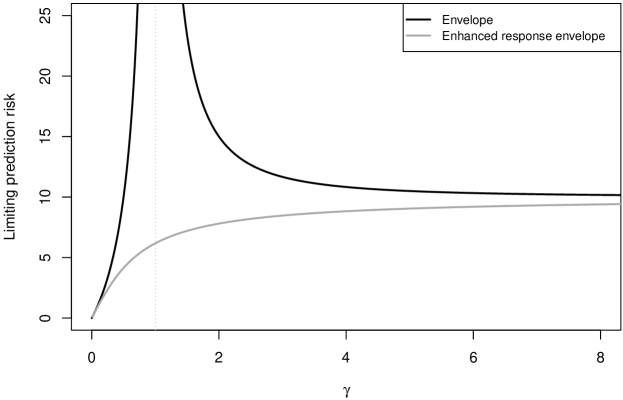
Figure 1: The limiting prediction risks of the enhanced response envelope with $\lambda^{\ast}={{\rm tr}}(\bm{\Omega})\gamma/c^{2}$ (gray solid line) and the envelope (black solid line), illustrating Theorem 2 when ${{\rm tr}}(\bm{\Omega})=10$ and ${{\rm tr}}(\bm{\beta}^{T}\bm{\beta})=10$.

Figure 1 visualizes the limiting prediction risk curves in Theorem 2. It plots the limiting risks of envelope (black solid line) and the enhanced response envelope with $\lambda^{\ast}={{\rm tr}}(\bm{\Omega})\gamma/c^{2}$ (dark-gray solid line), when ${{\rm tr}}(\bm{\Omega})=10$ and ${{\rm tr}}(\bm{\eta}^{T}\bm{\eta})=10$.

We have four remarks from Theorem 2. The limiting risk of envelope increases before $\gamma=1$ and then decreases after $\gamma=1$. The double descent phenomenon has been observed in popular methods such as neural networks, kernel machines and ridgeless regression (Belkin et al., 2019; Hastie et al., 2022), but this is the first time that such a result is established in the envelope literature. Second, the enhanced response envelope estimator always has a better asymptotic prediction risk than the envelope estimator (for any $c^{2}$, ${{\rm tr}}(\bm{\Omega})$, and $\gamma$). Third, in Theorem 1, we show the existence of a $\lambda$ that gives a smaller prediction risk of the enhanced response envelope than the envelope estimator. In an asymptotic regime, we specify such a $\lambda$ value: $\lambda^{\ast}={{\rm tr}}(\bm{\Omega})\gamma/c^{2}$. Lastly, the gap between two limiting prediction risks, $\lim_{n,p\rightarrow\infty}R(\hat{\bm{\beta}}_{\bm{\Gamma}}|\mathbf{X})$ and ${}_{n,p\rightarrow\infty}R(\hat{\bm{\beta}}_{\bm{\Gamma}}(\lambda^{\ast})|\mathbf{X})$, increases as $\gamma$ increases from $0$ to $1$. It is easy to see as $\frac{1}{1-\gamma}>m(-\lambda^{\ast})$, $0<\gamma<1$.

4 Simulation

In this section, we use simulations to compare the performance of the enhanced response envelope estimator and the envelope estimator in terms of the prediction risk, ${{\rm E}}[\|\hat{\bm{\beta}}\mathbf{x}_{\rm new}-\bm{\beta}\mathbf{x}_{\rm new}\|^{2}|\mathbf{X}]={{\rm tr}}[(\hat{\bm{\beta}}-\bm{\beta})\text{Cov}(\mathbf{x}_{\rm new})(\hat{\bm{\beta}}-\bm{\beta})^{T}]$. In addition, we use simulations to have a numeric illustration of the double descent phenomenon to confirm the asymptotic theory.

We consider a setting where $\mathbf{y}_{i}\in\mathbb{R}^{3}$ is generated from the model

$$\mathbf{y}_{i}=\bm{\beta}\mathbf{x}_{i}+\bm{\varepsilon}_{i},~{}\bm{\varepsilon}_{i}\sim N(\mathbf{0},\bm{\Sigma}),~{}i=1,\ldots,n,$$

and $\mathbf{x}_{i}\in\mathbb{R}^{p}$ is generated independently from $\mathbf{x}_{i}\sim N(\mathbf{0},\bm{\Sigma}_{\mathbf{x}}(\rho))$ where $(i,j)$th element of $\bm{\Sigma}_{\mathbf{x}}(\rho)\in\mathbb{R}^{p\times p}$ is $\rho^{|i-j|}$. The covariance matrix $\bm{\Sigma}$ is set using three orthonormal vectors and has eigenvalues $10$, $8$ and $2$. The columns of $\bm{\Gamma}$ are the second and third eigenvectors of $\bm{\Sigma}$. Each component of $\tilde{\bm{\eta}}\in\mathbb{R}^{2\times p}$ is generated from the standard normal distribution. We then set $\bm{\eta}=\sqrt{10}\cdot\tilde{\bm{\eta}}/\|\tilde{\bm{\eta}}\|_{F}$. In this setting, ${{\rm tr}}(\bm{\eta}^{T}\bm{\eta})=10$, ${{\rm tr}}(\bm{\Omega})=10$, and ${{\rm tr}}(\bm{\Omega}_{0})=10$. We assume that $\text{dim}(\mathcal{E}_{\bm{\Sigma},\mathcal{B}})=2$ is known.

Prediction risk comparison In this simulation, we try different combinations of $n$, $p$ and $\rho$ where $n\in\{50,90,200,500\}$, $p/n\in\{0.1,0.8,1.2\}$ and $\rho\in\{0,0.8\}$. We compare the prediction risk of the enhanced response envelope estimator to three different estimators: the envelope estimator, multivariate linear regression, and multivariate ridge regression.

For the enhanced response envelope and the multivariate ridge regression, we perform ten-fold cross-validation on simulated data to select $\lambda$ among equally spaced 100 candidate $\lambda$-values in the scale of logarithm base 10. We compute the envelope estimator for data with $n\leq p{-}r$ by taking a very small value of $\lambda=10^{-8}$ in the enhanced response envelope estimator. We fit multivariate regression model to $n<p$ data by taking a tiny value of $\lambda=10^{-8}$ in the multivariate ridge regression. We then calculate the prediction risk. This process is repeated $100$ times.

In Table 1, we report the prediction risk averaged over $100$ replications. First, we see that the prediction risks from the enhanced response envelope are consistently smaller than the envelope, as indicated in Theorem 1. Second, the enhanced response envelope consistently gives smaller prediction risks compared to the multivariate ridge regression. When $u=r$, the enhanced response envelope model reduces to the multivariate ridge regression. Therefore, the prediction risk of the enhanced envelope model can be smaller than that of multivariate ridge regression as long as ${{\rm tr}}(\bm{\Omega}_{0})>0$.

n	p	Enhanced envelope	Envelope	Multivariate linear reg	Multivariate ridge reg
Example 1:  $p/n=0.1$, $\rho=0$
50	5	1.31 (0.11)	1.40 (0.12)	2.39 (0.17)	2.04 (0.12)
90	9	1.24 (0.08)	1.41 (0.10)	2.33 (0.13)	1.92 (0.09)
200	20	1.16 (0.04)	1.26 (0.05)	2.31 (0.05)	1.93 (0.04)
500	50	1.06 (0.03)	1.18 (0.03)	2.28 (0.04)	1.85 (0.04)
Example 2:  $p/n=0.8$, $\rho=0$
50	40	6.73 (0.18)	60.89 (5.80)	104.45 (7.09)	7.16 (0.11)
90	72	6.44 (0.14)	55.10 (2.93)	94.81 (3.24)	7.05 (0.08)
200	160	5.86 (0.10)	42.50 (0.99)	81.33 (1.63)	6.91 (0.06)
500	400	5.67 (0.04)	40.61 (0.85)	79.17 (1.11)	6.89 (0.03)
Example 3:  $p/n=1.2$, $\rho=0$
50	60	8.02 (0.23)	33.70 (1.33)	93.79 (3.83)	8.08 (0.11)
90	108	7.58 (0.13)	41.01 (1.36)	94.38 (3.60)	7.98 (0.07)
200	240	7.02 (0.07)	47.91 (1.18)	99.94 (2.83)	7.82 (0.04)
500	600	6.78 (0.04)	50.43 (0.91)	103.33 (1.55)	7.75 (0.03)
Example 4:  $p/n=0.1$, $\rho=0.8$
50	5	1.76 (0.11)	1.98 (0.19)	2.39 (0.17)	1.84 (0.07)
90	9	1.02 (0.05)	1.40 (0.08)	2.33 (0.13)	1.45 (0.06)
200	20	0.90 (0.03)	1.30 (0.04)	2.31 (0.05)	1.31 (0.03)
500	50	0.78 (0.02)	1.19 (0.03)	2.28 (0.04)	1.22 (0.02)
Example 5:  $p/n=0.8$, $\rho=0.8$
50	40	4.16 (0.17)	62.50 (6.34)	104.45 (7.09)	4.76 (0.12)
90	72	3.78 (0.15)	55.14 (2.85)	94.81 (3.24)	4.63 (0.10)
200	160	3.32 (0.05)	42.40 (0.99)	81.33 (1.63)	4.28 (0.05)
500	400	3.09 (0.03)	40.69 (0.87)	79.17 (1.11)	4.05 (0.03)
Example 6:  $p/n=1.2$, $\rho=0.8$
50	60	5.24 (0.23)	36.43 (1.12)	104.17 (4.37)	5.80 (0.14)
90	108	4.41 (0.12)	44.84 (1.68)	103.01 (4.03)	5.16 (0.09)
200	240	4.05 (0.07)	51.46 (1.30)	109.34 (3.17)	4.98 (0.06)
500	600	3.86 (0.03)	54.21 (0.98)	112.62 (1.71)	4.82 (0.03)

Table 1: Prediction risk, averaged over $100$ replications. The standard error is given in parentheses. For $n\leq p{-}r$ data, we compute the envelope by taking a very small value of $\lambda=10^{-8}$ in the enhanced response envelope; see the definition of the envelope estimator (LABEL:eq:est-env-extstd) in Section 2.3. For $n<p$ data, we fit the multivariate regression model by taking a tiny value of $\lambda=10^{-8}$ in the multivariate ridge regression.

Double descent confirmation This simulation is designed to support Theorem 2 and to illustrate the double descent phenomenon in the envelope model. We set $n\in\{200,2000\}$ and $\rho=0$. $p/n$ varies from $0.1$ to $8$. We compute the envelope and the enhanced response envelope with setting $\lambda^{\ast}={{\rm tr}}(\bm{\Omega})p/(nc^{2})=p/n$ on simulated data. We then calculate the prediction risk for each estimator. Again, we fit $n\leq p{-}r$ data to the envelope estimator by taking a very small value of $\lambda=10^{-8}$ in the enhanced response envelope estimator.

Figure 2 displays the prediction risks from $n=2000$ with various $p$ values. The gray rectangle points denote the prediction risk for the enhanced response envelope estimator. The black triangle points are the prediction risk for the envelope estimator. We see a fascinating double descent prediction risk curve for the envelope model, as discussed in Theorem 2. Also, the enhanced response envelope gives a smaller prediction risk across the entire range of $p/n$. Figure 3 plots the prediction risk curves from $n=200$. We see that Figure 3 exhibits the same messages for the much smaller sample size. Although Theorem 2 is established when considering $\mathcal{E}_{\bm{\Sigma},\mathcal{B}}$ is known, we did not use this information in the actual estimation in the simulation study, yet the core message of Theorem 2 is confirmed by the simulation.

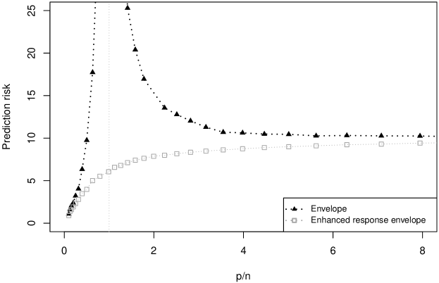
Figure 2: Prediction risk of the envelope and the enhanced response envelope with $\lambda^{\ast}={{\rm tr}}(\bm{\Omega})p/(nc^{2})$, when $n=2000$ and $p$ varies. For $n\leq p{-}r$ data, we fit the envelope by taking a very small value of $\lambda=10^{-8}$ in the enhanced response envelope estimator; see the definition of the envelope estimator (LABEL:eq:est-env-extstd) in Section 2.3.

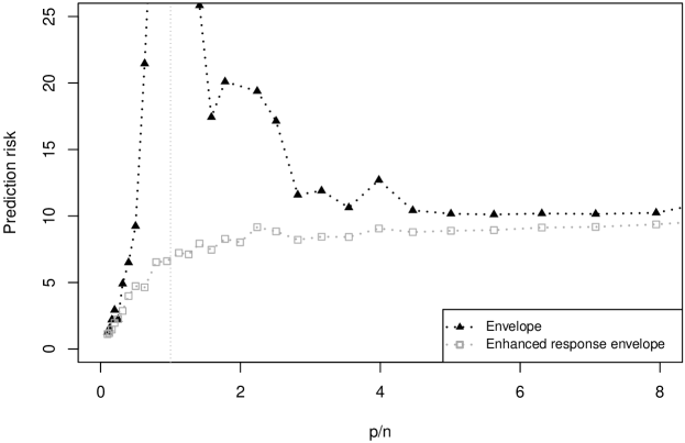
Figure 3: Prediction risk of the envelope and the enhanced response envelope with $\lambda^{\ast}={{\rm tr}}(\bm{\Omega})p/(nc^{2})$, when $n=200$ and $p$ varies. For $n\leq p{-}r$ data, we fit the envelope by taking a very small value of $\lambda=10^{-8}$ in the enhanced response envelope estimator; see the definition of the envelope estimator (LABEL:eq:est-env-extstd) in Section 2.3.

5 Real data

In this section, we use two real datasets to illustrate the enhanced response envelope estimator. We use air pollution data in which the number of samples is bigger than the number of predictors ($n>p$) in the next subsection. In Subsection 5.2, we analyze near-infrared spectroscopy data in which the number of predictors is much bigger than the number of predictors ($p\gg n$).

We compare the prediction performance of the enhanced response envelope estimator to the envelope estimator, multivariate regression, and multivariate ridge regression.

5.1 Air pollution data

The air pollution data are available and obtained directly from Table 1.5 of Johnson et al. (2002). The response vector $\mathbf{y}\in\mathbb{R}^{5}$ consists of atmospheric concentrations of CO, NO, NO₂, O₃, and HC, recorded at noon in the Los Angeles area on $42$ different days. The two predictors are wind speed and solar radiation. This data were analyzed in Cook (2018) to illustrate the effectiveness of the original envelope model compared to the standard multivariate regression model. They showed that the asymptotic standard errors of estimated components of $\bm{\beta}$ from the envelope model are significantly reduced compared to those from the standard multivariate regression model. We use the data to predict atmospheric concentrations from wind speed and solar radiation and compare the prediction performance of the enhanced response envelope estimator to the envelope estimator, the standard multivariate regression, and multivariate ridge regression.

To compare the prediction performance, we borrow the nested cross validation idea (Wang and Zou, 2021; Bates et al., 2021), in which an inner cross-validation is performed to tune a model and an outer cross-validation is performed to provide a prediction error of the tuned model. We adopt the leave-one-out cross-validation (LOOCV) procedure for the outer loop because the LOOCV error is an unbiased estimator of the generalization error of the tuned model and is shown to have nice performance compared to other methods for estimating generalization errors (Wang and Zou, 2021).

We take the $i$th observation out from the data and set the remaining $n{-}1$ observations as the training set to fit and tune models. We standardize $\mathbf{X}$ of the training set so that each column has a mean of 0 and a standard deviation of 1. We perform ten-fold cross-validation to select $(u,\lambda)$ from a fine grid of $u\in\{0,\ldots,5\}$ and $20$ equally spaced candidate $\lambda$-values in the scale of logarithm base 10 for the enhanced response envelope. For the envelope, we perform ten-fold cross-validation to choose $u$ from $\{0,\ldots,5\}$. For the multivariate ridge model, ten-fold cross-validation is performed to select $\lambda$ from $20$ equally spaced $\lambda$-values in the scale of logarithm base 10. The $i$th observation we take out at the beginning is set as the test set. We standardize $\mathbf{x}_{i}$ of the test set using the mean and standard deviation of the training data. We then calculate the squared prediction error, $\|\mathbf{y}_{i}-\hat{\bm{\beta}}^{(-i)}\mathbf{x}_{i}\|_{2}^{2}/r$, where $\hat{\bm{\beta}}^{(-i)}$ is the estimated regression coefficient derived from the training set. We repeat this process for $i=1,\ldots,n$ and report $\sum_{i=1}^{n}\|\mathbf{y}_{i}-\hat{\bm{\beta}}^{(-i)}\mathbf{x}_{i}\|_{2}^{2}/(nr)$ in Table 2. We see that the enhanced response envelope estimator gives the smallest prediction error among all competitors.

	Enhanced envelope	Envelope	Multivariate linear reg	Multivariate ridge reg
Error	8.859	8.951	9.192	9.124

Table 2: Air pollution data: prediction error of the enhanced response envelope method, the original envelope method, the multivariate linear regression, and the multivariate ridge regression.

5.2 Near-infrared spectroscopy data of fresh cattle manure

Near-infrared spectroscopy data of cattle manure were collected by Gogé et al. (2021). The data are available in the Data INRAE Repository at https://doi.org/10.15454/JIGO8R. This data contain 73 cattle manure samples that were analyzed by near-infrared spectroscopy using a NIRFlex device. Near-infrared spectra were recorded every 2 nm from 1100 to 2498 nm on fresh homogenized samples. In addition, the cattle manure samples were analyzed for three chemical properties: the amount of dry matter, magnesium oxide, and potassium oxide. We use the data of 62 cattle manure samples which have no missing values. We standardize each chemical property to have a sample mean of 0 and a standard deviation of 1. In our analysis, we consider the multivariate linear model, where $\mathbf{x}_{i}\in\mathbb{R}^{700}$ is the vector of near-infrared spectroscopy measurements and $\mathbf{y}_{i}\in\mathbb{R}^{3}$ is the vector of three chemical measurements to predict the three chemical properties from the absorbance spectra.

In Table 3, we report the prediction error which is calculated using the same procedure described in the previous subsection, except that $u$ is chosen from $\{0,\ldots,3\}$. Again, We see that the enhanced response envelope estimator has the smallest prediction error among all competitors.

	Enhanced envelope	Envelope	Multivariate linear reg	Multivariate ridge reg
Error	0.437	0.460	0.692	0.492

Table 3: Near-infrared spectroscopy data: prediction error from the enhanced response envelope method, the envelope method, the multivariate linear regression, and the multivariate ridge regression. We compute the envelope estimator by taking a very small value of $\lambda=10^{-8}$ in the enhanced response envelope estimator; see the definition of the envelope estimator (LABEL:eq:est-env-extstd) in Section 2.3. We fit the multivariate regression model by taking a very small value of $\lambda=10^{-8}$ in the multivariate ridge regression.

6 Discussion

In this paper, we have developed a novel envelope regularization function which is used to define the enhanced envelope estimator. We have shown that the enhanced envelope estimator is indeed better than the un-regularized envelope estimator in prediction. The asymptotic analysis of the risk function of envelope reveals, for the first time in the envelope literature, an interesting double descent phenomenon. The numeric examples in this work also suggest that the enhanced response envelope estimator is a promising new tool for multivariate regression.

Although this paper is focused on the case where the number of responses $(r)$ is less than the number of samples and the number of predictors, it is interesting to consider the case when $r\rightarrow\infty$ in ultrahigh-dimensional problems. Su et al. (2016) studied the response envelope for $r\rightarrow\infty$ but $p$ is fixed. When both $p,r>n$ and diverge, there are additional technical issues to be addressed. For example, we may need another penalty term to handle the issues caused by the large $r$ in the model. This direction of research will be investigated in a separate paper.

Appendix A Proofs of Theorems

A.1 Proof of Theorem 1

Note that

$$R(\hat{\bm{\beta}}_{\bm{\Gamma}}(\lambda)|\mathbf{X})=\lambda^{2}{{\rm tr}}(\bm{\beta}(\mathbf{S}_{\mathbf{X}}+\lambda\mathbf{I})^{-1}\bm{\Sigma}_{\mathbf{x}}(\mathbf{S}_{\mathbf{X}}+\lambda\mathbf{I})^{-1}\bm{\beta}^{T})+\frac{{{\rm tr}}(\bm{\Omega})}{n}{{\rm tr}}(\bm{\Sigma}_{\mathbf{x}}\mathbf{S}_{\mathbf{X}}(\mathbf{S}_{\mathbf{X}}+\lambda\mathbf{I})^{-2}).$$

Therefore, we have

$$\frac{\partial}{\partial\lambda}R(\hat{\bm{\beta}}_{\bm{\Gamma}}(\lambda)|\mathbf{X})$$

$$=2\lambda\cdot{{\rm tr}}(\bm{\beta}\mathbf{S}_{\mathbf{X}}(\mathbf{S}_{\mathbf{X}}+\lambda\mathbf{I})^{-2}\bm{\Sigma}_{\mathbf{x}}(\mathbf{S}_{\mathbf{X}}+\lambda\mathbf{I})^{-1}\bm{\beta}^{T})-2\frac{{{\rm tr}}(\bm{\Omega})}{n}{{\rm tr}}(\bm{\Sigma}_{\mathbf{x}}\mathbf{S}_{\mathbf{X}}(\mathbf{S}_{\mathbf{X}}+\lambda\mathbf{I})^{-3})$$

$$\leq\sum_{i=1}^{p}\left(2\lambda\cdot\sigma_{i}(\bm{\beta}^{T}\bm{\beta})-2\frac{{{\rm tr}}(\bm{\Omega})}{n}\right)\sigma_{i}(\bm{\Sigma}_{\mathbf{x}}\mathbf{S}_{\mathbf{X}}(\mathbf{S}_{\mathbf{X}}+\lambda\mathbf{I})^{-3}),$$

where $\sigma_{i}(\mathbf{M})$ denotes the $i$-th largest eigenvalue of $\mathbf{M}$. The inequality above comes from Von Neumann’s trace inequality.

Since $\frac{\partial}{\partial\lambda}R(\hat{\bm{\beta}}_{\bm{\Gamma}}(\lambda)|\mathbf{X})<0$ if $\lambda<{{\rm tr}}(\bm{\Omega})/(n\sigma_{1}\left(\bm{\beta}^{T}\bm{\beta})\right)$, $R(\hat{\bm{\beta}}_{\bm{\Gamma}}(\lambda)|\mathbf{X})$ is a monotonically decreasing function if $0\leq\lambda\leq{{\rm tr}}(\bm{\Omega})/(n\sigma_{1}\left(\bm{\beta}^{T}\bm{\beta})\right)$. Therefore, we have

$$R(\hat{\bm{\beta}}_{\bm{\Gamma}}(\lambda)|\mathbf{X})<\frac{{{\rm tr}}(\bm{\Omega})}{n}{{\rm tr}}(\bm{\Sigma}_{\mathbf{x}}\mathbf{S}_{\mathbf{X}}^{+}),$$

when $0<\lambda<{{\rm tr}}(\bm{\Omega})/(n\sigma_{1}\left(\bm{\beta}^{T}\bm{\beta})\right)$. Since

$$\frac{{{\rm tr}}(\bm{\Omega})}{n}{{\rm tr}}(\bm{\Sigma}_{\mathbf{x}}\mathbf{S}_{\mathbf{X}}^{+})\leq R(\hat{\bm{\beta}}_{\bm{\Gamma}}|\mathbf{X}),$$

we prove the theorem.

A.2 Proof of Theorem 2

Our analyses of limiting prediction risk follow that of Hastie et al. (2022).

As $\bm{\Sigma}_{\mathbf{x}}=\mathbf{I}$,

$$R(\hat{\bm{\beta}}_{\bm{\Gamma}}|\mathbf{X})={{\rm vec}}^{T}(\bm{\beta})[\Pi_{\mathbf{X}}\otimes\mathbf{I}_{r}]{{\rm vec}}(\bm{\beta})+\frac{{{\rm tr}}(\bm{\Omega})}{n}{{\rm tr}}(\mathbf{S}_{\mathbf{X}}^{+}),$$

$$R(\hat{\bm{\beta}}_{\bm{\Gamma}}(\lambda)|\mathbf{X})=\lambda^{2}{{\rm tr}}(\bm{\beta}(\mathbf{S}_{\mathbf{X}}+\lambda\mathbf{I})^{-2}\bm{\beta}^{T})+\frac{{{\rm tr}}(\bm{\Omega})}{n}{{\rm tr}}(\mathbf{S}_{\mathbf{X}}(\mathbf{S}_{\mathbf{X}}+\lambda\mathbf{I})^{-2}),$$

where $\Pi_{\mathbf{X}}=\mathbf{I}_{p}-\mathbf{S}_{\mathbf{X}}^{+}\mathbf{S}_{\mathbf{X}}$.

A.2.1 Proof for envelope estimator when $\gamma<1$

Let us consider the case where $p/n\rightarrow\gamma\in(0,1)$. From Theorem 1 of Bai and Yin (2008), $\sigma_{\min}(\mathbf{S}_{\mathbf{X}})\geq(1-\sqrt{\gamma})^{2}/2$ and $\sigma_{\max}(\mathbf{S}_{\mathbf{X}})\leq 2(1+\sqrt{\gamma})^{2}$ almost surely for all sufficiently large $n$. Therefore, in this case, $\mathbf{S}_{\mathbf{X}}$ is invertible and the bias term of $R(\hat{\bm{\beta}}_{\bm{\Gamma}}|\mathbf{X})$ is 0, almost surely.

The variance term of $R(\hat{\bm{\beta}}_{\bm{\Gamma}}|\mathbf{X})$ is

$$\frac{{{\rm tr}}(\bm{\Omega})}{n}{{\rm tr}}(\mathbf{S}_{\mathbf{X}}^{+})=\frac{p\cdot{{\rm tr}}(\bm{\Omega})}{n}\int\frac{1}{s}dF_{\mathbf{S}_{\mathbf{X}}}(s),$$

where $F_{\mathbf{S}_{\mathbf{X}}}(s)$ is the spectral measure of $\mathbf{S}_{\mathbf{X}}$. By the Marchenko-Pastur theorem, which says that $F_{\mathbf{S}_{\mathbf{X}}}\rightarrow F_{\gamma}$, and the Portmanteau theorem,

$$\int_{(1-\sqrt{\gamma})^{2}/2}^{2(1+\sqrt{\gamma})^{2}/}\frac{1}{s}dF_{\mathbf{S}_{\mathbf{X}}}(s)\rightarrow\int_{(1-\sqrt{\gamma})^{2}/2}^{2(1+\sqrt{\gamma})^{2}/}\frac{1}{s}dF_{\gamma}(s)=\int\frac{1}{s}dF_{\gamma}(s).$$

The equality is because the support of $F_{\gamma}$ is $[(1-\sqrt{\gamma})^{2},(1+\sqrt{\gamma})^{2}]$. We can also remove the upper and lower limits of integration on the left-hand side by Theorem 1 of Bai and Yin (2008). Thus, combining above results, we arrive at

$$R(\hat{\bm{\beta}}_{\bm{\Gamma}}|\mathbf{X})\rightarrow\gamma\cdot{{\rm tr}}(\bm{\Omega})\int\frac{1}{s}dF_{\gamma}(s).$$

The Stieltjes transformation of $F_{\gamma}$ is given by

$$m(z)=\int\frac{1}{s-z}dF_{\gamma}(s)=\frac{(1-\gamma-z)-\sqrt{(1-\gamma-z)^{2}-4\gamma z})}{2\gamma z},$$

for any real $z<0$. By taking the limit $z\rightarrow 0^{-}$, the proof is completed.

A.2.2 Proof for envelope estimator when $\gamma>1$

The variance term of $R(\hat{\bm{\beta}}_{\bm{\Gamma}}|\mathbf{X})$ is

$$\frac{{{\rm tr}}(\bm{\Omega})}{n}{{\rm tr}}(\mathbf{S}_{\mathbf{X}}^{+})=\frac{{{\rm tr}}(\bm{\Omega})}{n}{{\rm tr}}((\mathbf{X}\mathbf{X}^{T}/n)^{+})=\frac{{{\rm tr}}(\bm{\Omega})}{p}{{\rm tr}}((\mathbf{X}\mathbf{X}^{T}/p)^{+}).$$

Considering $n/p\rightarrow\tau=1/\gamma<1$, by the same arguments from the proof above, we conclude that

$$\frac{{{\rm tr}}(\bm{\Omega})}{n}{{\rm tr}}(\mathbf{S}_{\mathbf{X}}^{+})\rightarrow{{\rm tr}}(\bm{\Omega})\frac{1}{\gamma-1}.$$

Let $\bm{\beta}=[\mathbf{b}_{1}^{T}~{}\ldots~{}\mathbf{b}_{r}^{T}]$. The bias term is

$${{\rm vec}}^{T}(\bm{\beta})[\Pi_{\mathbf{X}}\otimes\mathbf{I}_{r}]{{\rm vec}}(\bm{\beta})=\sum_{i=1}^{r}\mathbf{b}_{i}^{T}\Pi_{\mathbf{X}}\mathbf{b}_{i}=\sum_{i=1}^{r}\lim_{z\rightarrow 0^{+}}z\mathbf{b}_{i}^{T}(\mathbf{S}_{\mathbf{X}}+z\mathbf{I})^{-1}\mathbf{b}_{i}.$$

From Theorem 1 of Bai et al. (2007), we have that

$$z\mathbf{b}_{i}^{T}(\mathbf{S}_{\mathbf{X}}+z\mathbf{I})^{-1}\mathbf{b}_{i}\rightarrow z\int\frac{1}{s+z}F_{\gamma}(s)=z\|\mathbf{b}_{i}\|^{2}m(-z)~{}\text{ a.s.},$$

for any $i=1,\ldots,r$. We further have that

$$\sum_{i=1}^{r}z\mathbf{b}_{i}^{T}(\mathbf{S}_{\mathbf{X}}+z\mathbf{I})^{-1}\mathbf{b}_{i}\rightarrow zc^{2}m(-z)~{}\text{ a.s}.$$

By the Arzela-Ascoli theorem and the Moore-Osgood theorem, we exchange limits and arrive at

$$\lim_{z\rightarrow 0^{+}}\sum_{i=1}^{r}z\mathbf{b}_{i}^{T}(\mathbf{S}_{\mathbf{X}}+z\mathbf{I})^{-1}\mathbf{b}_{i}\rightarrow c^{2}\lim_{z\rightarrow 0^{+}}zm(-z)=c^{2}(1-1/\gamma)~{}\text{ a.s}.$$

Combining the variance and the bias terms, we complete the proof.

A.2.3 Proof for enhanced envelope estimator

We use the similar techniques from the envelope estimator for both variance and bias terms. The variance term of $R(\hat{\bm{\beta}}_{\bm{\Gamma}}(\lambda))$ becomes

$$\frac{{{\rm tr}}(\bm{\Omega})}{n}{{\rm tr}}(\mathbf{S}_{\mathbf{X}}(\mathbf{S}_{\mathbf{X}}+\lambda\mathbf{I})^{-2})\rightarrow\gamma{{\rm tr}}(\bm{\Omega})\int\frac{s}{(s+\lambda)^{2}}F_{\gamma}(s).$$

Let $g_{n,\lambda}(\eta)=\lambda\cdot{{\rm tr}}(\bm{\beta}(\mathbf{S}_{\mathbf{X}}+\lambda(1+\eta)\mathbf{I})^{-1}\bm{\beta}^{T}),~{}\eta\in[-1/2,1/2]$. The bias term of $R(\hat{\bm{\beta}}_{\bm{\Gamma}}(\lambda))$ is

$$\lambda^{2}{{\rm tr}}(\bm{\beta}(\mathbf{S}_{\mathbf{X}}+\lambda\mathbf{I})^{-2}\bm{\beta}^{T})=-\frac{\partial}{\partial\eta}g_{n}(\lambda,0).$$

Because

$$g_{n,\lambda}(\eta)\rightarrow\lambda c^{2}m(-\lambda(1+\eta))=\lambda c^{2}\int\frac{1}{s+\lambda(1+\eta)}dF_{\gamma}(s),$$

and derivative and limit are exchangeable, we have that

$$\lambda^{2}{{\rm tr}}(\bm{\beta}(\mathbf{S}_{\mathbf{X}}+\lambda\mathbf{I})^{-2}\bm{\beta}^{T})\rightarrow\lambda^{2}c^{2}\int\frac{1}{(s+\lambda)^{2}}dF_{\gamma}(s).$$

We can conclude that,

$$R(\hat{\bm{\beta}}_{\bm{\Gamma}}(\lambda))\rightarrow\int\frac{\lambda^{2}c^{2}+s\cdot\gamma{{\rm tr}}(\bm{\Omega})}{(s+\lambda)^{2}}F_{\gamma}(s).$$

The right-hand side is minimized at $\lambda^{\ast}=\gamma{{\rm tr}}(\bm{\Omega})/c^{2}$. In such case, the right-hand side becomes $\gamma{{\rm tr}}(\bm{\Omega})\cdot m(-\lambda^{\ast})$.

References

- Bai et al. (2007) Bai, Z., Miao, B., and Pan, G. (2007), “On asymptotics of eigenvectors of large sample covariance matrix,” The Annals of Probability, 35, 1532–1572.
- Bai and Yin (2008) Bai, Z.-D. and Yin, Y.-Q. (2008), “Limit of the smallest eigenvalue of a large dimensional sample covariance matrix,” in Advances In Statistics, World Scientific, pp. 108–127.
- Bates et al. (2021) Bates, S., Hastie, T., and Tibshirani, R. (2021), “Cross-validation: what does it estimate and how well does it do it?” arXiv preprint arXiv:2104.00673.
- Belkin et al. (2019) Belkin, M., Hsu, D., Ma, S., and Mandal, S. (2019), “Reconciling modern machine-learning practice and the classical bias–variance trade-off,” Proceedings of the National Academy of Sciences, 116, 15849–15854.
- Chun and Keleş (2010) Chun, H. and Keleş, S. (2010), “Sparse partial least squares regression for simultaneous dimension reduction and variable selection,” Journal of the Royal Statistical Society: Series B (Statistical Methodology), 72, 3–25.
- Cook (2018) Cook, R. (2018), An Introduction to Envelopes: Dimension Reduction for Efficient Estimation in Multivariate Statistics, Wiley Series in Probability and Statistics, Wiley.
- Cook and Forzani (2019) Cook, R. D. and Forzani, L. (2019), “Partial least squares prediction in high-dimensional regression,” The Annals of Statistics, 47, 884–908.
- Cook et al. (2016) Cook, R. D., Forzani, L., and Su, Z. (2016), “A note on fast envelope estimation,” Journal of Multivariate Analysis, 150, 42–54.
- Cook et al. (2015) Cook, R. D., Forzani, L., and Zhang, X. (2015), “Envelopes and reduced-rank regression,” Biometrika, 102, 439–456.
- Cook et al. (2013) Cook, R. D., Helland, I., and Su, Z. (2013), “Envelopes and partial least squares regression,” Journal of the Royal Statistical Society: Series B (Statistical Methodology), 75, 851–877.
- Cook et al. (2007) Cook, R. D., Li, B., and Chiaromonte, F. (2007), “Dimension reduction in regression without matrix inversion,” Biometrika, 94, 569–584.
- Cook et al. (2010) — (2010), “Envelope models for parsimonious and efficient multivariate linear regression,” Statistica Sinica, 927–960.
- Cook and Su (2013) Cook, R. D. and Su, Z. (2013), “Scaled envelopes: scale-invariant and efficient estimation in multivariate linear regression,” Biometrika, 100, 939–954.
- Cook and Su (2016) — (2016), “Scaled predictor envelopes and partial least-squares regression,” Technometrics, 58, 155–165.
- Cook and Zhang (2015a) Cook, R. D. and Zhang, X. (2015a), “Foundations for envelope models and methods,” Journal of the American Statistical Association, 110, 599–611.
- Cook and Zhang (2015b) — (2015b), “Simultaneous envelopes for multivariate linear regression,” Technometrics, 57, 11–25.
- De Jong (1993) De Jong, S. (1993), “SIMPLS: an alternative approach to partial least squares regression,” Chemometrics and intelligent laboratory systems, 18, 251–263.
- Ding and Cook (2018) Ding, S. and Cook, R. D. (2018), “Matrix variate regressions and envelope models,” Journal of the Royal Statistical Society: Series B (Statistical Methodology), 80, 387–408.
- Ding et al. (2020) Ding, S., Su, Z., Zhu, G., and Wang, L. (2020), “Envelope quantile regression,” Statistica Sinica.
- Dobriban and Wager (2018) Dobriban, E. and Wager, S. (2018), “High-dimensional asymptotics of prediction: Ridge regression and classification,” The Annals of Statistics, 46, 247–279.
- El Karoui (2018) El Karoui, N. (2018), “On the impact of predictor geometry on the performance on high-dimensional ridge-regularized generalized robust regression estimators,” Probability Theory and Related Fields, 170, 95–175.
- Gogé et al. (2021) Gogé, F., Thuriès, L., Fouad, Y., Damay, N., Davrieux, F., Moussard, G., Le Roux, C., Trupin-Maudemain, S., Valé, M., and Morvan, T. (2021), “Dataset of chemical and near-infrared spectroscopy measurements of fresh and dried poultry and cattle manure,” Data in Brief, 34, 106647.
- Hastie et al. (2022) Hastie, T., Montanari, A., Rosset, S., and Tibshirani, R. J. (2022), “Surprises in high-dimensional ridgeless least squares interpolation,” The Annals of Statistics, 50, 949–986.
- Johnson et al. (2002) Johnson, R. A., Wichern, D. W., et al. (2002), Applied multivariate statistical analysis, vol. 5, Prentice hall Upper Saddle River, NJ.
- Khare et al. (2017) Khare, K., Pal, S., and Su, Z. (2017), “A bayesian approach for envelope models,” The Annals of Statistics, 196–222.
- Li and Zhang (2017) Li, L. and Zhang, X. (2017), “Parsimonious tensor response regression,” Journal of the American Statistical Association, 112, 1131–1146.
- Liang and Rakhlin (2020) Liang, T. and Rakhlin, A. (2020), “Just Interpolate: Kernel “Ridgeless” Regression can generalize,” Annals of Statistics, 48, 1329–1347.
- Rekabdarkolaee et al. (2020) Rekabdarkolaee, H. M., Wang, Q., Naji, Z., and Fuente, M. (2020), “NEW PARSIMONIOUS MULTIVARIATE SPATIAL MODEL,” Statistica Sinica, 30, 1583–1604.
- Rimal et al. (2019) Rimal, R., Almøy, T., and Sæbø, S. (2019), “Comparison of multi-response prediction methods,” Chemometrics and Intelligent Laboratory Systems, 190, 10–21.
- Su and Cook (2011) Su, Z. and Cook, R. D. (2011), “Partial envelopes for efficient estimation in multivariate linear regression,” Biometrika, 98, 133–146.
- Su and Cook (2013) — (2013), “Estimation of multivariate means with heteroscedastic errors using envelope models,” Statistica Sinica, 213–230.
- Su et al. (2016) Su, Z., Zhu, G., Chen, X., and Yang, Y. (2016), “Sparse envelope model: efficient estimation and response variable selection in multivariate linear regression,” Biometrika, 103, 579–593.
- Wang and Zou (2021) Wang, B. and Zou, H. (2021), “Honest leave-one-out cross-validation for estimating post-tuning generalization error,” Stat, 10, e413.
- Zhang and Li (2017) Zhang, X. and Li, L. (2017), “Tensor envelope partial least-squares regression,” Technometrics, 59, 426–436.
- Zhao et al. (2022) Zhao, Y., Van Keilegom, I., and Ding, S. (2022), “Envelopes for censored quantile regression,” Scandinavian Journal of Statistics.
- Zhu and Su (2020) Zhu, G. and Su, Z. (2020), “Envelope-based sparse partial least squares,” The Annals of Statistics, 48, 161–182.