Padding Module: Learning the Padding in Deep Neural Networks

Abstract

During the last decades, many studies have been dedicated to improving the performance of neural networks, for example, the network architectures, initialization, and activation. However, investigating the importance and effects of learnable padding methods in deep learning remains relatively open. To mitigate the gap, this paper proposes a novel trainable Padding Module that can be placed in a deep learning model. The Padding Module can optimize itself without requiring or influencing the model’s entire loss function. To train itself, the Padding Module constructs a ground truth and a predictor from the inputs by leveraging the underlying structure in the input data for supervision. As a result, the Padding Module can learn automatically to pad pixels to the border of its input images or feature maps. The padding contents are realistic extensions to its input data and simultaneously facilitate the deep learning model’s downstream task. Experiments have shown that the proposed Padding Module outperforms the state-of-the-art competitors and the baseline methods. For example, the Padding Module has 1.23% and 0.44% more classification accuracy than the zero padding when tested on the VGG16 and ResNet50.

I Introduction

Deep Neural Networks (DNNs) have significantly improved the performance of a wide range of computer vision tasks to the extent of being comparable to or exceeding human-level in many domains [1], such as image classification [2], object recognition [3], and image segmentation [4]. DNNs for computer vision have been iteratively improving in different aspects such as network architecture [5, 6, 7, 8], network initialization [9, 10], optimization [11, 12], and activation [13, 14]. While it is intuitive that the salient foreground of an input image can control the results of a deep learning model [15, 16], researchers have also discovered that the input’s borders and corners can dominate the model’s performance recently [17, 18, 19]. The study on the importance and effects of image borders remains relatively open, and this paper focuses on a trainable padding method that process image borders for deep learning models.

Padding refers to the technique of adding extra data to the input’s borders so that the input’s width, height, or depth can be manipulated. Padding is widely used in Convolutional Neural Networks (CNNs) to alter the output size of a convolutional layer. Without padding, convolutional filters will not process the input’s borders and the output size will be reduced. The input size can be maintained with padding; we add an extra border before the convolution so that the original border can be processed [20].

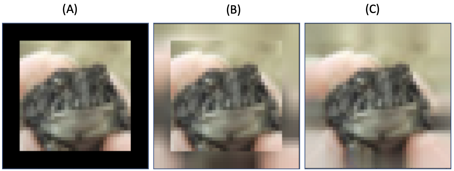
Figure 1: Five-pixel padding applied to a CIFAR-10 sampled image using three different padding methods: A) the zero padding, B) the local mean interpolation, and C) the proposed Padding Module.

Traditional padding techniques include zero padding, replication padding, and reflection padding. The reflection padding reflects the valid data over the borders; the replication padding uses the borders themselves as padding values; the zero padding specifies the use of zeroes as padding values. The replication and reflection padding methods extend the input with duplicate contents that may not be realistic; hence, they may destroy the original distribution [19]. The zero padding may outweigh the replication and reflection padding methods in terms of speed due to its computational simplicity. The major drawback of the traditional methods is that they are not dynamic. Thus, the padding values are always static and not optimized during the model training in a way that how they could be optimally predicted rationally to the input’s borders.

More recently, padding methods have been studied aiming at a more related and realistic extension of the original input [21, 19]. For example, Liu et al. [21] proposed a padding method using partial convolution. Nguyen et al. [19] used a local mean of a sliding window over the input’s borders so the local distributions at the borders before and after the padding are consistent. These state-of-the-art padding methods outperformed the traditional padding in several tasks such as image classification, image segmentation, and image style transfer. However, the major disadvantage of the state-of-the-art padding methods is that they are not trainable: the padding contents are still not optimized.

In this paper, we propose a trainable Padding Module that can be inserted into selected positions of a deep learning model to learn how to pad its inputs. The Padding Module can be trained simultaneously with a deep learning model, but, it is a self-learner in a way that will not require or influence the model’s entire loss function. During the training, the Padding Module internally constructs a ground truth from the input’s actual borders and trains a predictor considering the neighboring areas. The trained Padding Module can produce plausible results, as shown in Figure 1. The advantages of our work can be summarized as three-fold:

• The proposed Padding Module introduces a trainable method that automatically pads its inputs.

• The Padding Module extends its input with realistic new data that are related to the original data.

• The Padding Module improves the performance of a downstream task of a deep learning model and outperforms the state-of-the-art competitors, e.g., classification.

The remainder of this paper is organized as follows. In Section II, we review the related work that addressed the padding effects on the neural networks performance and discuss how the current study fills the gap in the related work. Section III discusses our approach for the Padding Module followed by evaluation results in Section IV. Finally, Section V concludes with the discussion on evaluation and highlights some of the future work in this sector.

II Literature Review and Related Work

Many studies have tried to improve the performance of CNNs models from network architecture [22, 23, 24, 25], different variants of optimization [26, 27, 28], activations [29, 30, 31, 32], regularization methods [33, 34] and so no. However, little attention has been paid to investigating the padding schemes during the convolution operation. To assist the kernel, i.e., features extractor, in extracting important features during image processing in CNNs, padding layers can be added to visit pixels of the images around the corners more times, and then increase accuracy. The previous padding methods are presented as follows: Section II-A presents the performance improvement of neural networks; Section II-B introduces the improvement of space design; and Section II-C describes our contributions.

II-A Performance Improvement of Neural Networks

Several studies have proposed padding methods to improve the performance of the neural networks [21, 19, 17].

Innamorati et al. [17] addressed the importance of the data at the borders of the input by proposing a convolution layer that dealt with corners and borders separately from the middle part of the image. They specifically designed filters for each corner and border to handle the data at the boundaries, including upper, lower, left, and right borders. The boundary filters used in the convolution were jointly learned with the filter used for the middle part of the image. However, the main issue of this study is that the number of filters used to deal with the boundaries increases linearly with the size of the receptive field.

Also, Nguyen et al. [19] proposed a padding method that could keep the local spatial distribution of the padded area consistent with the original input. The proposed method used the local means of the input at the borders to produce the padding values; they proposed two different variants of the padding method: mean-interpolation and mean-reflection. Both variants used filters with static values, based on the receptive field, in the convolution operation that is supposed to yield the padding values maintaining the same distributions as the original borders. However, the main issue with this method is that they are not learnable.

Liu et al. [21] proposed a padding layer that uses a partial convolution that mainly re-weighted the convolution operation based on the ratio of the number of parameters in the filter to the number of valid data in the sliding window. In other words, they dealt with the padded area as hole areas that need to be in-painted, while the data coming from the original image were seen as non-hole areas. The main issue of this study is that the padding process is not learnable.

II-B Improvement of Spaces Design

Also, some studies addressed the importance of the padding and data at the boundaries in the semantic representation learning and converting 360-degree space to 2-dimensional (2-D) space respectively [35, 36, 37].

Cheng et al. [37] showed the importance of the padding method when they converted the 360-degree video to 2-dimensional space. They converted the video to six faces. Then, they used the reflection padding to connect them to form the 2-D space. The reflection padding naturally connected the faces compared to the zero-padding, which caused discontinuity.

Interesting works were provided by Islam et al. [35, 36] in which they showed the importance of zero padding along with the data at the borders in encoding the absolute position information in the semantic representation learning. They showed that the zero padding and the boundaries drove the CNN models to encode the spatial information that helped the filters where to look for a specific feature; the spatial information was eventually propagated over the whole image.

II-C Our Contributions

The padding methods and their effects on a CNN model’s performance are still open areas for researchers to investigate; hence, it is worth proposing new padding methods that could improve the performance of the CNN models. We propose a novel padding method, Padding Module, that could realistically extend the input with related data. It learns how to pad the input by using the inputs’ borders as a ground truth and the neighboring areas of the borders as a predictor. Then, it uses a local loss function such as Mean Squared Error (MSE) and updates the filters using the local differentiation of the loss function with respect to the Padding Module’s filters. The following section explains the implementation of the Padding Module.

III The proposed Padding Module

This paper presents the Padding Module, a learnable padding method that can pad the input with related and realistic padding, as shown in Figure 1. The Padding Module can be used as a substitute for other padding methods in the convolution layer, such as the zero padding, the replication padding, and the reflection padding. This section shows how the padding procedure (Section III-A) and the backpropagation (Section III-B) of the Padding Module work.

III-A Padding Procedure

Algorithms 1 and 2, respectively, give an overview of the forward pass and the back-propagation of the Padding Module. The Padding Module first constructs a ground truth and a predictor from the input ( shown in step $1$ to step $3$ in Algorithm 1 and explained in Sections III-A1 and III-A2). Then, the Padding Module uses the filters being learned to produce the actual padding values using the input’s borders as a predictor ( shown in steps $4$ to $13$ in Algorithm 1 and explained in Section III-A4). Finally, the Padding Module uses the MSE as a loss function to compute the loss value and updates the filters during the model’s back-propagation ( shown in steps $1$ to $2$ in Algorithm 2 and explained in Sections III-A3 and III-B).

The Padding Module can pad the original input with any padding size, ($e.g.,$ one-pixel, two-pixels, etc). Indeed, the padding process in the Padding Module is iterative ( shown in steps $4$ to $13$ in Algorithm 1). Assume the required padding size is three pixels, the padding process will iterate three times as follows: (1) padding the original input with one-pixel along all the four borders; (2) padding the output of the $1^{st}$ iteration with one-pixel along all the four borders; and (3) padding the output of the $2^{nd}$ iteration with one-pixel along all the four borders. Here, to easily explain our method, a simple case of padding process was presented here, $e.g.,$ one-pixel padding. Also, the Padding Module is assigned filters as many as the number of channels in the input as explained in Section III-A3. Then, we explain the padding process considering a single channel. Here, the same procedure is separately applied to each channel in case of multiple channels.

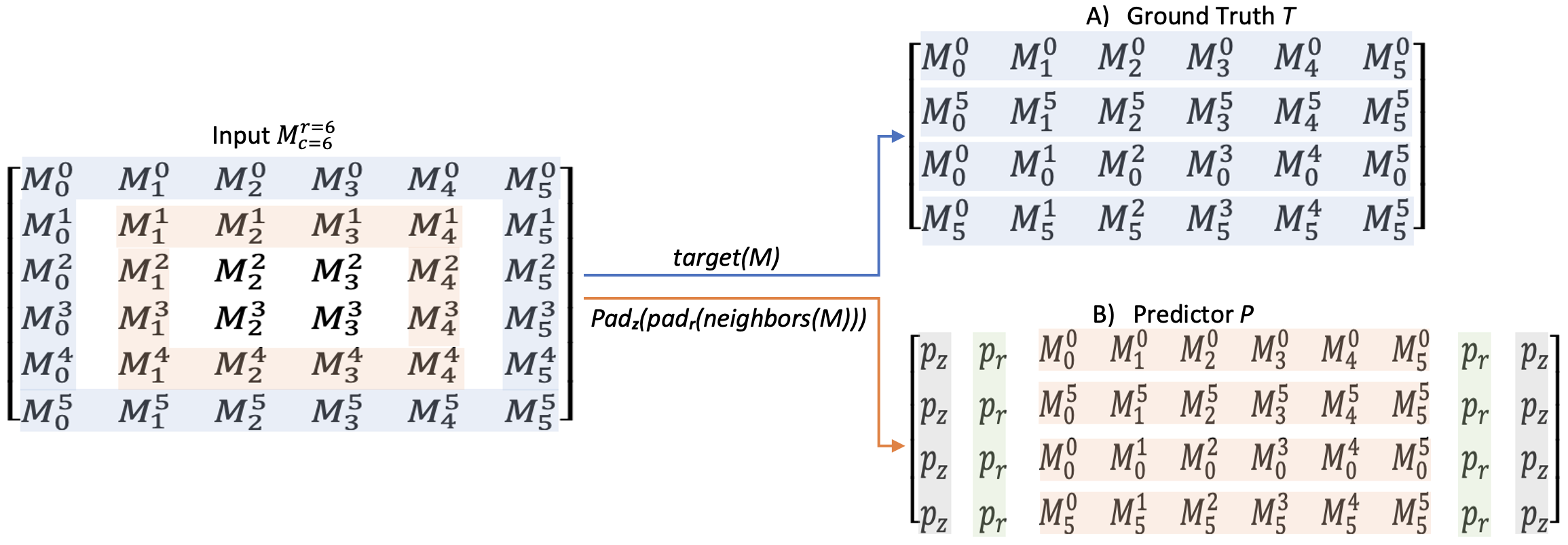
Figure 2: An example to illustrate the steps 1-3 in Algorithm 1. On the left: the input $M_{c}^{r}$ with size of $(6,6)$ pixels; the superscripts are the indexes in the row-wise traversal while the subscripts are the indexes in the column-wise traversal of the input. On the right: (A) the ground truth $T$: a result of applying step $1$ in Algorithm 1 which is a stack of the borders where the first row, second row, third row, and last row are the upper, lower, left, and right borders in the input respectively; and (B) the predictor $P$: a result of applying steps $2$ and $3$ in Algorithm 1 which is a stack of the neighbors where the first row, second row, third row, and last row are neighbors to the upper, lower, left, and right borders in the input respectively, and the stack is padded at the left and right sides with reflection padding ($p_{r}$) and with zero padding ($p_{z}$).

Algorithm 1 Forward Pass

1:$M_{c}^{r}$, $size$, where $r$ and $c$ are the dimensions of a matrix, and $size$ is the padding size.

2:${M_{c^{\prime}}^{r^{\prime}}}$, where $r^{\prime}=r+2\times size$, and $c^{\prime}=c+2\times size$.

3:$T\leftarrow target(M_{c}^{r})$ /* as in Eq.1 */

4:$N\leftarrow neighbors(M_{c}^{r})$ /* as in Eq.2 */

5:$P\leftarrow pad_{z}(pad_{r}(N))$ /* as in Eq.3 */

6:$M_{c^{\prime}}^{r^{\prime}}\leftarrow M_{c}^{r}$/* initial state for $\overline{M_{c^{\prime}}^{r^{\prime}}}$ */

7:while $size\not=0$ do

8:     $Nout\leftarrow borders(M_{c^{\prime}}^{r^{\prime}})$ /* as in Eq.6 */

9:     $Pout\leftarrow pad_{z}(pad_{r}(Nout))$ /* as in Eq.3 */

10:     $O\leftarrow f_{\theta}(Pout)$ /* as in Eq. 7 */

11:     $M_{c^{\prime}+2}^{r^{\prime}+2}\leftarrow O^{0}//pad_{z}(M_{c^{\prime}}^{r^{\prime}})//O^{1}$

12:     $M_{c^{\prime}+2}^{r^{\prime}+2}\leftarrow sides((O^{2})^{T},M_{c^{\prime}+2}^{r^{\prime}+2},(O^{3})^{T})$ /* as in Eq.8 */

13:     $M_{c^{\prime}}^{r^{\prime}}\leftarrow corners(M_{c^{\prime}+2}^{r^{\prime}+2})$ /* as in Eq.9 */

14:     $size\leftarrow size-1$

15:end while

16:return $M_{c^{\prime}}^{r^{\prime}}$

Algorithm 2 Back Propagation

1:$G_{c^{\prime}}^{r^{\prime}}$, where $c^{\prime}$ and $r^{\prime}$ are the same dimensions of the output of the forward pass in Algorithm 1.

2:$G_{c}^{r}$, where $c$ and $r$ are the same dimensions of the input of the forward pass in Algorithm 1.

3:Compute the local gradients. /* as in Eq.5 */

4:Update the filter weights

5:$G_{c}^{r}\leftarrow strip(G_{c^{\prime}}^{r^{\prime}})$ /* as in Eq.10 */

6:return $G_{c}^{r}$

III-A1 Ground Truth $T$

The Padding Module structures the ground truth $T$ by extracting the input’s borders and stacking them upon each other vertically to form a four-row matrix. However, to stack the left and right borders vertically in $T$, they are transposed from column vectors to row vectors. Formally, given $M_{c}^{r}$ as an original input with $r$ and $c$ as the number of rows and columns respectively; henceforth, superscripts and subscripts represent the indexes in the row-wise traversal and the column-wise traversal of the input respectively. The following is $T$’s extracting function $target$ of the input $M_{c}^{r}$:

$$T=target(M_{c}^{r})=\begin{bmatrix}M_{[:]}^{0}\\ M_{[:]}^{r-1}\\ {(M_{0}^{[:]})}^{T}\\ {(M_{c-1}^{[:]})}^{T}\end{bmatrix},$$ (1)

where $M_{[:]}^{0}$ is the entire row vector in $M_{c}^{r}$ at index $0$, $M_{[:]}^{r-1}$ is the entire row vector in $M_{c}^{r}$ at index $r-1$, ${(M_{0}^{[:]})}^{T}$ is the transpose of the entire column vector in $M_{c}^{r}$ at index $0$, and ${(M_{c-1}^{[:]})}^{T}$ is the transpose of the entire column vector in $M_{c}^{r}$ at index $c-1$. Figure 2. (A) is an example to visually illustrate how $T$ is constructed where the first row represents the upper border in $M_{c}^{r}$, the second row represents the lower border in $M_{c}^{r}$, the third row represents the left border in $M_{c}^{r}$, and the last row represents the right border in $M_{c}^{r}$.

III-A2 Predictor ($P$)

To structure the predictor from the original input $M_{c}^{r}$, the Padding Module extracts the row vectors that neighbor the upper border and lower border in $M_{c}^{r}$ and the transpose of the column vectors that neighbor the left border and right border in $M_{c}^{r}$. Then, the Padding Module stacks all the extracted neighbors vertically to form a four-row matrix. Formally, the predictor’s (denoted as $P$) extracting function of $M_{c}^{r}$ can be expressed in the following way:

First, the neighbors in $M_{c}^{r}$ are selected and denoted as $N$ as follows:

$$N=neighbors(M_{c}^{r})=\begin{bmatrix}M_{[1:c-1]}^{1}\\ M_{[1:c-1]}^{r-2}\\ {(M_{1}^{[1:r-1]})}^{T}\\ {(M_{c-2}^{[1:r-1]})}^{T}\end{bmatrix}.$$ (2)

The slice $[1:c-1]$ excludes the data in the row vectors at the borders due to overlapping with the $T$, whereas the slice $[1:r-1]$ excludes the data in the column vectors at the borders due to overlapping with $T$.

Then, the Padding Module pads the structure as follows:

$$P=pad_{z}(pad_{r}(N)).$$ (3)

First, the $pad_{r}(.)$ function pads the structure with one pixel of the reflection padding horizontally (the left and right sides); then, with one pixel of the zero padding horizontally using the $pad_{z}(.)$ function can get the final structure for $P$.

Each row in $P$ will be used to predict the corresponding row in $T$. For example, the first row in $P$ will be used to predict the first row in $T$ representing the upper border in the input $M_{c}^{r}$. Figure 2 (B) is an example to visually illustrate how the Padding Module constructs the stack of the neighbors (as a predictor) where the right and left sides of the stack are padded with the reflection padding (named as $p_{r}$), and the zero padding (named as $p_{z}$).

III-A3 Filters and the Loss Function

The Padding Module uses as many filters as the channels in the input (i.e., filter per channel). Also, each filter will be a row vector with a size of $(1,3)$ and a stride of $(1,1)$; that is because of having each row in $P$ as a predictor for the corresponding row in $T$. Therefore, to predict $T$, the Padding Module convolutes the filters over $P$; it uses its own loss function to optimize the prediction through the local differentiation of the loss function with respect to the filters.

The loss function used by the Padding Module is the MSE which computes the squared difference between the ground truth and the predicted value. The following equation is the MSE’s mathematical expression for a single data point:

$$MSE(f_{\theta}(P),T)=\sum_{a=1}^{4}\sum_{j=1}^{n}(\theta^{T}\cdot P^{a}_{j}-T^{a}_{j})^{2},$$ (4)

where $f$ is the convolutional operation parameterized by ${\theta}$, $P$ and $T$ are the predictor and the ground truth extracted from the original input $M_{c}^{r}$, $a$ represents the indexes for rows in the four-row matrices $P$ and $T$, and $j$ represents the indexes for both the slide windows and columns in $P$ and $T$ respectively. Hence, $P^{a}_{j}$ is the $j$th slide window in the row indexed at $a$ in $P$, and $T^{a}_{j}$ is the corresponding value in $T$ indexed at the $a$th row and $j$th column.

The local differentiation of the Padding Module’s loss function and the filters’ updates are achieved during the model’s back-propagation; these local gradients are not propagated to the previous layer. Besides that, the Padding Module facilities the back-propagation of the model’s loss function going through it to the previous layer as explained in Section III-B. The following is the mathematical expression for the local gradients (Padding Module’s loss function gradients with respect to a single filter for a single data point):

$$\frac{\varphi}{\varphi\theta_{m}}MSE(f_{\theta}(P),T)=2\sum_{a=1}^{4}\sum_{j=1}^{n}(\theta^{T}\cdot P^{a}_{j}-T^{a}_{j})x_{m},$$ (5)

where $x_{m}$ is a single feature in the $P^{a}_{j}$ slide window which was multiplied by the corresponding weight, namely $\theta_{m}$, in the $\theta$ during the convolution.

III-A4 Padding Process

The procedures in Sections III-A1, III-A2, and III-A3 are used to guide the Padding Module on learning how to predict the borders of the original input, $M_{c}^{r}$, based on the neighboring areas to the borders, and then the Padding Module can optimize its filters.

However, the padding process is shown in steps $4$ to $13$ in Algorithm 1; it uses the borders of the input, $M_{c^{\prime}}^{r^{\prime}}$, as the predictor. In detail, the padding process iterates until the original input is padded with the required padding size. Hence, the original input $M_{c}^{r}$ is assigned to $M_{c^{\prime}}^{r^{\prime}}$ as an initial state in step $4$ before the padding loop starts. Then, each iteration pads the input, $M_{c^{\prime}}^{r^{\prime}}$, with one-pixel, and outputs a new $M_{c^{\prime}}^{r^{\prime}}$ which will be used for the next iteration and so forth. The dimensions of an iteration’s output, $M_{c^{\prime}}^{r^{\prime}}$ in step $11$, are two-pixel larger than the dimensions of that iteration’s input, $M_{c^{\prime}}^{r^{\prime}}$ in step $6$.

Minutely, constructing the predictor in the padding process is similar to the way that constructs $P$ in Section III-A2 with small modifications. To distinguish the notions of $neighbors$, $N$, and $P$, in Section III-A2, $borders$, $Nout$, and $Pout$ are denoted for the extracting function, the function’s output, and the predictor, respectively. The following is the mathematical expression for the extracting function $borders$:

$$Nout=borders(M_{c^{\prime}}^{r^{\prime}})=\begin{bmatrix}M_{[:]}^{0}\\ M_{[:]}^{r-1}\\ {(M_{0}^{[:]})}^{T}\\ {(M_{c-1}^{[:]})}^{T}\end{bmatrix},$$ (6)

where $M_{[:]}^{0}$ and $M_{[:]}^{r-1}$ mean extracting the entire upper and lower borders respectively. Whereas, $(M_{0}^{[:]})^{T}$ and $(M_{c-1}^{[:]})^{T}$ mean extracting the transpose of the entire left and right borders respectively. Then, the Padding Module pads the output $Nout$ using Equation 3 to get the final structure for $Pout$.

Consequently, convoluting the filters over the $Pout$ will produce the padding values for the iteration’s input. The output can be expressed as follows:

$$O=f_{\theta}(Pout),$$ (7)

where $f$ is the convolutional operation parameterized by ${\theta}$, $Pout$ is the predictor, and the $O$ is the output and comes as a matrix of four rows. Each row represents the padding values for the corresponding area in the iteration’s input, $M_{c^{\prime}}^{r^{\prime}}$, as follows: the first row ($O^{0}$), the second row ($O^{1}$), the third row ($O^{2}$), and the fourth row ($O^{3}$) represent the padding values for the upper, the lower, the left, and the right areas in the input respectively.

Then, the steps from $9$ to $11$ are how the produced padding values stick around the input $M_{c^{\prime}}^{r^{\prime}}$. First, in step $9$, the vertical concatenation operator $//$ is used to concatenate the first row ($O^{0}$) with $M_{c^{\prime}}^{r^{\prime}}$, and then concatenates the resulted matrix with the second row ($O^{1}$). However, the rows from $O$ are two-pixel wider than the rows of $M_{c^{\prime}}^{r^{\prime}}$; therefore, to match the dimensions of these operands, the Padding Module uses $pad_{z}(.)$ to pad the $M_{c^{\prime}}^{r^{\prime}}$ horizontally with one pixel of the zero padding before the concatenation process. Hence, the output’s dimensions in step $9$, denoted as $M_{c^{\prime}+2}^{r^{\prime}+2}$, are two-pixel larger than the input $M_{c^{\prime}}^{r^{\prime}}$. Finally, the algorithm uses $sides$ function which can be formally expressed as the following:

$$sides((O^{2})^{T},M_{c^{\prime}+2}^{r^{\prime}+2},(O^{3})^{T}).$$ (8)

This function does not change the dimensions; however, it adds respectively the transpose of the third row ($O^{2}$) and fourth row ($O^{3}$) to the left and right columns of $M_{c^{\prime}+2}^{r^{\prime}+2}$, the concatenated matrix with zero values at the left and right columns unless the corners already assigned values from the concatenation process. To resolve the double-count problem at the corners, the Padding Module takes the average of added values in the corners by dividing each corner by $2$; this averaging function is step $12$ in Algorithm 1:

$$M_{c^{\prime}}^{r^{\prime}}=corners(M_{c^{\prime}+2}^{r^{\prime}+2}).$$ (9)

Lastly, as mentioned early in this section that the dimensions of the iteration’s output are two-pixel larger than the iteration’s input. Hence, the output $M_{c^{\prime}}^{r^{\prime}}$, in Equation 9, has dimensions $r^{\prime}$ and $c^{\prime}$ that are updated with the dimensions of $M_{c^{\prime}+2}^{r^{\prime}+2}$, namely $r^{\prime}+2$ and $c^{\prime}+2$ respectively.

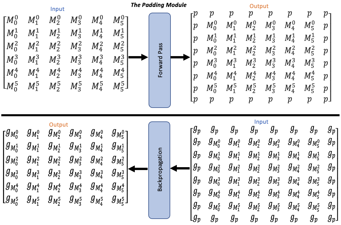
Figure 3: An example to illustrate the back propagation in Algorithm 2. On the top: the input to the Padding Module is of size $(6,6)$, the Padding Module uses one-pixel padding and produces an output of size $(8,8)$ where the borders $p$ is the computed padding values. On the bottom: the back-propagation of the received gradients which is of size $(8,8)$ where the borders are gradients for the padding values $g_{p}$; the Padding Module strips out $g_{p}$ from the received gradients, and sends the remaining to the previous layer. The $g$ stands for gradient; for example $g_{M_{0}^{0}}$ is the gradient for the pixel at index $[0,0]$ in the input of the Forward Pass.

III-B Back-propagation

As seen in Section III-A3, the Padding Module is not optimized based on the model’s main loss function; therefore, the model does not compute the gradients of its loss function with respect to the filters of the Padding Module. However, during the mode’s backpropagation, the Padding Module achieves two key points as follows:

1. As shown in step $1$ in Algorithm 2, the Padding Module optimizes its filters through computing the local gradients for its loss function with respect to the filters as explained in Section III-A3.

2. The process also receives $G_{c^{\prime}}^{r^{\prime}}$ which are the gradients of the model’s loss function with respect to the Padding Module’s output, the original input $M_{c}^{r}$ after being padded. Therefore, the Padding Module strips out the gradients from $G_{c^{\prime}}^{r^{\prime}}$ that represent the gradients for the padded areas in the Padding Module’s output; the stripping-out process is step $3$ in Algorithm 2, and formally expressed as follows:

   $$G_{c}^{r}=strip(G_{c^{\prime}}^{r^{\prime}}).$$ (10)

   Then, the Padding Module back-propagates to the previous layer the $G_{c}^{r}$, representing the gradients for the previous layer’s output. Figure 3 is an example to visually illustrate how the back-propagation process in the Padding Module is achieved.

IV Experimental Results and Analysis

This section shows the design of the training and testing experiments on our Padding Module applied to a downstream task, i.e., image classification. The experimental setup is presented in Sections IV-A. The quantitative and qualitative results are described in Section IV-B and IV-C.

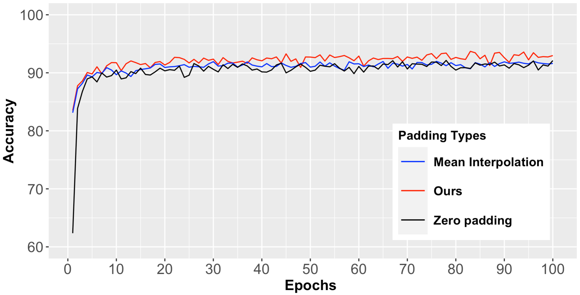
Figure 4: The comparison of three different padding methods on the test images: zero padding, mean interpolation padding, and the Padding Module when applied to the VGG16 model.

Figure 5: The comparison of three different padding methods on the test images: zero padding, mean interpolation padding, and the Padding Module when applied to the ResNet50V2.

IV-A Experiment Setup

The study used the premium service from Google Colaboratory where a GPU of Tesla T4 was assigned. The experiments and comparisons were conducted on the CIFAR-10 dataset for a classification task [38]. The CIFAR-10 dataset includes a training dataset of 50,000 images and a test dataset of 10,000 images. The images are of shape $(32,32,3)$, distributed equally to ten classes of airplane, automobile, bird, cat, deer, dog, frog, horse, ship, and truck. The Padding Module was applied to different networks namely: VGG16 [8] and ResNet50V2 [39]; to make the deeper layers in these networks carry out a valid convolution, the images were resized to $(64,64,3)$ and $(224,224,3)$ for the VGG16 and the ResNet50V2, respectively.

The VGG16 is a vanilla-based architecture where the network shape is wider at the beginning of the network and narrowed down as going deep in the network. The pre-trained VGG16 was obtained from the keras without the top layers (the last three dense layers including the original softmax layer). Then, we added two fully-connected layers each with 512 neurons and followed by a dropout layer. On the other hand, the ResNet50V2 is made up of blocks where each block sends the block’s input through the block itself, and also uses a skip connection to directly add the block’s input to the output of the input’s flow coming through the block. The process is known as the identity function that could help deep layers to improve the model’s accuracy. ResNet50V2 is a modified version of the ResNet50 [13]. The modification mainly is in the arrangement of the block layers; batch normalization [11] and ReLU activation [40] are applied to the data flow before the convolutional layer in the block. These changes enabled the ResNet50V2 to outperform the ResNet50 on the image classification task. The ResNet50V2 was downloaded from the keras without the top layer (the last dense layer which is the original softmax layer). Then, two fully-connected layers with $1024$ and $512$ neurons were added.

Moreover, we added a softmax layer with ten outputs for both models of VGG16 and ResNet50V2, and then used the Adam optimizer [12] for the back-propagation of the gradients. Finally, the Padding Module was used before every convolutional layer in the VGG16; whereas, we replaced every zero padding layer in the ResNet50V2 with the Padding Module.

IV-B Quantitative Results

Section IV-B1 compares the proposed Padding Module and state-of-art padding solutions by performing the image classification task, and then Section IV-B2 discusses an ablation study based on our solution.

IV-B1 Image Classification Task

We considered the zero padding method as a baseline to compare the Padding Module with. Moreover, we used the mean interpolation padding method [19] as the state-of-art since it outperformed the partial convolution padding method [21, 19] in the image classification. The main goal of this study, which aligns with the literature, is to investigate the padding effect on the accuracy of DNN models. Therefore, the accuracy is used as a comparison metric between the performance of the Padding Module and the benchmark. The accuracy is the percentage of correctly classified images over the total number of images in the dataset.

Each model was trained with 100 epochs using the training dataset, and tested in each epoch using the test dataset. In Figure 4, the Padding Module outperforms both the baseline method and the mean interpolation padding method when using the VGG16; also, we found that the baseline is comparable to the mean interpolation method. As for the Resent50, the Padding Module also outperforms the other two paddings as shown in Figure 5. We also noticed that the baseline method is comparable to the mean interpolation method. Moreover, Table I summarizes the average of the last five epochs for the three different padding methods and the margin between the highest and the second-highest accuracies for the two models.

Padding Method	VGG16	ResNet50V2
Padding Module	92.92	95.08
Zero Padding	91.43	94.64
Mean Interoplation	91.69	94.44
margin	1.23	0.44

TABLE I: The average accuracy of the last five epochs for three different padding methods used in VGG16 and ResNet50V2. The margin is the difference between each model’s highest and second-highest padding methods.

As mentioned, the study investigated the effects of the Padding Module on the accuracy of DNN models. Importantly, we showed that the related and realistic padding could improve the accuracy of DNN models ; therefore, the Padding Module was able to produce such padding by minimizing the MSE in Algorithms 1 and 2. Figure 6 illustrates MSEs for three cases of the Padding Module applied in different places (at the beginning, in the middle, and at the end) in the VGG16; it is evident that the MSEs significantly decreased after only two epochs and then stayed flat till the end of the experiment for the three cases.

Figure 6: MSEs for three Padding Modules placed at different positions in the VGG16: 1) module 1: at the beginning, 2) module 2: at the middle, and 3) module 3: at the end.

One natural drawback of the current Padding Module was the extra running time caused by constructing the data structures and optimizing the filters. Table 2 shows that VGG16 and ResNet50V2, on average, doubled the epoch’s time when applying the Padding Module ($i.e.,$ placing the Padding Module before every convolutional layer in the VGG16 and replacing every zero padding layer in the ResNet50V2 with the Padding Module). On the other side, the accuracy for the VGG16 and ResNet50V2, respectively, gained margins of 1.49% and 0.44% when applying the Padding Module compared to the zero padding (no Padding Module). One remedy to lessen the running time problem may be to stop training the Padding Module when it significantly decreases the MSE after the first two epochs. However, improving the current Padding Module including the time complexity can be a further direction for further research.

IV-B2 Ablation Study

The experiments in this section were conducted as an ablation study where the Padding Module was empirically placed at different positions in the VGG16 model, as shown in Figure 7: at the beginning of the model, in the middle, at the end, and the combination of all the three places together. We also compared the four scenarios with two other scenarios: (1) where the Padding Module was placed in all positions (before each convolutional layer) in the model; and (2) where the Padding Module was not used but the zero padding was used instead. We ran each scenario 100 epochs using the training dataset for training and the test dataset for evaluation, and averaged the test accuracies of the last five epochs for each scenario; Table III illustrates the summary of the comparison of the models. We noticed that using a single Padding Module with the shallow layers outperformed the case of using it with the deep layers. Also, the combination scenario showed a superiority over the scenario of a single Padding Module. However, the best performance was when the Padding Module applied in the scenario of all positions. Finally, all the scenarios of applying the Padding Module outperformed the scenario of the model with no Padding Module.

Model	Zero Padding		Padding Module		Margin
	Accuracy	Time	Accuracy	Time
VGG16	91.43	2	92.92	4	1.49
ResNet50	94.64	5	95.08	9	0.44

TABLE II: On average, the running time doubles for one epoch when applying the Padding Module to the VGG16 and ResNet50V2 compared to the case of the zero padding (no Padding Module applied). Times are shown in a minute-scale. The margin is the accuracy difference between the case of applying the Padding Module and the zero padding.

No	Different places in the VGG16	Accuracy
1	At the beginning	91.98
2	At the middle	91.8
3	At the end	91.97
4	Combination of 1, 2, and 3 togather	92.18
5	All positions	92.8
6	VGG16 with no Padding Module	91.4

TABLE III: Placing the Padding Module at different positions in the VGG16: 1) at the beginning 2) at the middle 3) at the end 4) combination of beginning, middle, end 5) before every convolutional layer 6) VGG16 with no Padding Module (zero padding instead).

Figure 7: The selected positions in the VGG16 for the Padding Module: at the beginning, middle, and the end.

Figure 8: Three images sampled from CIFAR-10 and padded by different padding methods: zero-padding, mean interpolation, and the Padding Module. Each padding method uses three different padding sizes: A) one-pixel, B) three-pixel, C) five-pixel.

IV-C Qualitative Results

Different padding sizes, such as one-pixel, three-pixel, and five-pixel, were used to illustrate how the Padding Module can extend the input with related and realistic extensions. Also, we compared these different padding sizes with the other two methods, namely the zero padding and the mean interpolation padding. As shown in Figure 8, the Padding Module can learn how to pad the input with related data and natural extension; this finding becomes more evident as the padding size increases.

V Future Research Directions and Conclusion

This paper proposed a novel padding method: Padding Module; that can learn how to pad an input from the input’s borders; hence, the input can be realistically extended with related data. The Padding Module is a self-learning of its weights. To train itself, the Padding Module constructs a ground truth and a predictor from the inputs by leveraging the underlying structure in the input data for supervision. The Padding Module uses convolutional operation over the predictor to produce a predicted value that is, in turn, compared with the ground truth. The Padding Module uses a local loss function, independent from the model’s main loss function, to minimize the difference between the predicted value and the ground truth. Therefore, the Padding Module updates its convolutional filters locally during the model’s back-propagation. Besides that, the Padding Module back-propagates the model’s gradients with respect to the Padding Module’s output after stripping out the gradients for the padded areas to the previous layer.

The experimental results showed that the Padding Module outperformed the zero-padding and the state-of-art padding in the image classification task. In the ablation study, we also observed that using a single Padding Module with the shallow layers improved the performance slightly better than using it with the deep layers in the VGG16 network. On the other hand, using three of the Padding Module placed in different positions (at the beginning, at the middle, and at the end) in the VGG16 outperformed the scenario of a single Padding Module. Moreover, placing the Padding Module in all positions (before every convolutional layer) in the VGG16 outperformed all other scenarios as shown in Table III.

Our experiments applied the Padding Module to the two well-known networks: VGG16 and ResNet50, for the image classification task. The VGG16 and ResNet50 networks were chosen to represent small and large networks, respectively. They, also, were used by the literature; hence, we used them to compare the Padding Module with the previous work. Although two different networks are only used in one task, we shall extend the Padding Module to improve such networks in different tasks, including object detection, style transfer, and image inpainting. We leave investigating the Padding Module in a wide range of tasks for future research.

Also, the Padding Module learned how to pad the input independently of the model’s loss function. However, it is possible to optimize the Padding Module’s filters based on optimizing the model’s main loss function; this approach will be entirely different. Hence, one research direction may be to implement a padding method that can optimize its padding filters based on the model’s main loss function.

References

- [1] K. Eykholt, I. Evtimov, E. Fernandes, B. Li, A. Rahmati, C. Xiao, A. Prakash, T. Kohno, and D. Song, “Robust physical-world attacks on deep learning visual classification,” in Proceedings of the IEEE conference on computer vision and pattern recognition, 2018, pp. 1625–1634.
- [2] T. He, Z. Zhang, H. Zhang, Z. Zhang, J. Xie, and M. Li, “Bag of tricks for image classification with convolutional neural networks,” in Proceedings of the IEEE/CVF Conference on Computer Vision and Pattern Recognition, 2019, pp. 558–567.
- [3] J. Huang, V. Rathod, C. Sun, M. Zhu, A. Korattikara, A. Fathi, I. Fischer, Z. Wojna, Y. Song, S. Guadarrama et al., “Speed/accuracy trade-offs for modern convolutional object detectors,” in Proceedings of the IEEE conference on computer vision and pattern recognition, 2017, pp. 7310–7311.
- [4] K. He, G. Gkioxari, P. Dollár, and R. Girshick, “Mask r-cnn,” in Proceedings of the IEEE international conference on computer vision, 2017, pp. 2961–2969.
- [5] J. Kim, H. Zeng, D. Ghadiyaram, S. Lee, L. Zhang, and A. C. Bovik, “Deep convolutional neural models for picture-quality prediction: Challenges and solutions to data-driven image quality assessment,” IEEE Signal processing magazine, vol. 34, no. 6, pp. 130–141, 2017.
- [6] Y. Li, C. Fang, J. Yang, Z. Wang, X. Lu, and M.-H. Yang, “Universal style transfer via feature transforms,” Advances in neural information processing systems, vol. 30, 2017.
- [7] A.-D. Nguyen, S. Choi, W. Kim, and S. Lee, “A simple way of multimodal and arbitrary style transfer,” in ICASSP 2019-2019 IEEE International Conference on Acoustics, Speech and Signal Processing (ICASSP). IEEE, 2019, pp. 1752–1756.
- [8] K. Simonyan and A. Zisserman, “Very deep convolutional networks for large-scale image recognition,” arXiv preprint arXiv:1409.1556, 2014.
- [9] D. Arpit, V. Campos, and Y. Bengio, “How to initialize your network? robust initialization for weightnorm & resnets,” Advances in Neural Information Processing Systems, vol. 32, 2019.
- [10] K. He, X. Zhang, S. Ren, and J. Sun, “Delving deep into rectifiers: Surpassing human-level performance on imagenet classification,” in Proceedings of the IEEE international conference on computer vision, 2015, pp. 1026–1034.
- [11] S. Ioffe and C. Szegedy, “Batch normalization: Accelerating deep network training by reducing internal covariate shift,” in International conference on machine learning. PMLR, 2015, pp. 448–456.
- [12] D. P. Kingma and J. Ba, “Adam: A method for stochastic optimization,” CoRR, vol. abs/1412.6980, 2014.
- [13] K. He, X. Zhang, S. Ren, and J. Sun, “Deep residual learning for image recognition,” in Proceedings of the IEEE conference on computer vision and pattern recognition, 2016, pp. 770–778.
- [14] G. Huang, Z. Liu, L. Van Der Maaten, and K. Q. Weinberger, “Densely connected convolutional networks,” in Proceedings of the IEEE conference on computer vision and pattern recognition, 2017, pp. 4700–4708.
- [15] K. Simonyan, A. Vedaldi, and A. Zisserman, “Deep inside convolutional networks: Visualising image classification models and saliency maps,” arXiv preprint arXiv:1312.6034, 2013.
- [16] B. Zhou, A. Khosla, A. Lapedriza, A. Oliva, and A. Torralba, “Learning deep features for discriminative localization,” in Proceedings of the IEEE conference on computer vision and pattern recognition, 2016, pp. 2921–2929.
- [17] C. Innamorati, T. Ritschel, T. Weyrich, and N. J. Mitra, “Learning on the edge: Explicit boundary handling in cnns,” 2018.
- [18] G. Liu, K. J. Shih, T.-C. Wang, F. A. Reda, K. Sapra, Z. Yu, A. Tao, and B. Catanzaro, “Partial convolution based padding,” arXiv preprint arXiv:1811.11718, 2018.
- [19] A.-D. Nguyen, S. Choi, W. Kim, S. Ahn, J. Kim, and S. Lee, “Distribution padding in convolutional neural networks,” in 2019 IEEE International Conference on Image Processing (ICIP), 2019, pp. 4275–4279.
- [20] S. Albawi, T. A. Mohammed, and S. Al-Zawi, “Understanding of a convolutional neural network,” in 2017 International Conference on Engineering and Technology (ICET), 2017, pp. 1–6.
- [21] G. Liu, K. J. Shih, T.-C. Wang, F. A. Reda, K. Sapra, Z. Yu, A. Tao, and B. Catanzaro, “Partial convolution based padding,” 2018.
- [22] K. He, X. Zhang, S. Ren, and J. Sun, “Deep residual learning for image recognition,” in Proceedings of the IEEE conference on computer vision and pattern recognition, 2016, pp. 770–778.
- [23] G. Huang, Z. Liu, L. Van Der Maaten, and K. Q. Weinberger, “Densely connected convolutional networks,” in Proceedings of the IEEE conference on computer vision and pattern recognition, 2017, pp. 4700–4708.
- [24] T. Takikawa, D. Acuna, V. Jampani, and S. Fidler, “Gated-scnn: Gated shape cnns for semantic segmentation,” in Proceedings of the IEEE/CVF international conference on computer vision, 2019, pp. 5229–5238.
- [25] I. Radosavovic, R. P. Kosaraju, R. Girshick, K. He, and P. Dollár, “Designing network design spaces,” in Proceedings of the IEEE/CVF conference on computer vision and pattern recognition, 2020, pp. 10 428–10 436.
- [26] D. P. Kingma and J. Ba, “Adam: A method for stochastic optimization,” arXiv preprint arXiv:1412.6980, 2014.
- [27] S. Ioffe and C. Szegedy, “Batch normalization: Accelerating deep network training by reducing internal covariate shift,” in International conference on machine learning. PMLR, 2015, pp. 448–456.
- [28] L. Liu, H. Jiang, P. He, W. Chen, X. Liu, J. Gao, and J. Han, “On the variance of the adaptive learning rate and beyond,” arXiv preprint arXiv:1908.03265, 2019.
- [29] A. L. Maas, A. Y. Hannun, A. Y. Ng et al., “Rectifier nonlinearities improve neural network acoustic models,” in Proc. icml, vol. 30, no. 1. Atlanta, Georgia, USA, 2013, p. 3.
- [30] K. He, X. Zhang, S. Ren, and J. Sun, “Delving deep into rectifiers: Surpassing human-level performance on imagenet classification,” in Proceedings of the IEEE international conference on computer vision, 2015, pp. 1026–1034.
- [31] P. Ramachandran, B. Zoph, and Q. V. Le, “Searching for activation functions,” arXiv preprint arXiv:1710.05941, 2017.
- [32] M. A. Mercioni and S. Holban, “P-swish: Activation function with learnable parameters based on swish activation function in deep learning,” in 2020 International Symposium on Electronics and Telecommunications (ISETC). IEEE, 2020, pp. 1–4.
- [33] J. Tompson, R. Goroshin, A. Jain, Y. LeCun, and C. Bregler, “Efficient object localization using convolutional networks,” in Proceedings of the IEEE conference on computer vision and pattern recognition, 2015, pp. 648–656.
- [34] G. Larsson, M. Maire, and G. Shakhnarovich, “Fractalnet: Ultra-deep neural networks without residuals,” arXiv preprint arXiv:1605.07648, 2016.
- [35] M. A. Islam, S. Jia, and N. D. B. Bruce, “How much position information do convolutional neural networks encode?” 2020.
- [36] M. A. Islam, M. Kowal, S. Jia, K. G. Derpanis, and N. D. B. Bruce, “Position, padding and predictions: A deeper look at position information in cnns,” 2021.
- [37] H.-T. Cheng, C.-H. Chao, J.-D. Dong, H.-K. Wen, T.-L. Liu, and M. Sun, “Cube padding for weakly-supervised saliency prediction in 360 videos,” 2018.
- [38] A. Krizhevsky, G. Hinton et al., “Learning multiple layers of features from tiny images,” 2009.
- [39] K. He, X. Zhang, S. Ren, and J. Sun, “Identity mappings in deep residual networks,” in European conference on computer vision. Springer, 2016, pp. 630–645.
- [40] A. F. Agarap, “Deep learning using rectified linear units (relu),” arXiv preprint arXiv:1803.08375, 2018.