Feasibility and Regularity Analysis of Safe Stabilizing Controllers under Uncertainty

Abstract

This paper studies the problem of safe stabilization of control-affine systems under uncertainty. Our starting point is the availability of worst-case or probabilistic error descriptions for the dynamics, a control barrier function (CBF) and a control Lyapunov function (CLF). These descriptions give rise to second-order cone constraints (SOCCs) whose simultaneous satisfaction guarantees safe stabilization. We study the feasibility of such SOCCs and the regularity properties of various controllers satisfying them.

1 Introduction

The last years have seen a dramatic increase in the deployment of robotic systems in diverse areas like home automation and autonomous driving. In these applications, it is critical that robots satisfy simultaneously safety and performance specifications in the presence of model uncertainty. Controllers that achieve these goals are usually defined using tools from stability analysis and Lyapunov theory. However, this raises several challenges. Among them, we highlight understanding the level of uncertainty about the model that can be tolerated while still being able to meet safety and stability requirements, the characterization of the regularity properties of the controller, and the identification of suitable conditions to ensure them in order to be implementable in real-world scenarios.

Literature Review: Control Lyapunov functions (CLFs) (Artstein, 1983) are a well-established tool for designing stabilizing controllers for nonlinear systems. More recently, control barrier functions (CBFs) (Wieland and Allgöwer, 2007; Ames et al., 2019) have been introduced as a tool to render a certain predefined set safe. If the system is control affine, the CLF and CBF conditions can be incorporated in a quadratic program (QP) (Ames et al., 2017) that can be efficiently solved online. Several recent works (Cortez and Dimarogonas, 2021; Ong and Cortés, 2019; Reis et al., 2021; Mestres and Cortés, 2023) study the feasibility of such CLF-CBF QP, as well as different explicit control designs based on it. However, this design assumes complete knowledge of the dynamics and safe set. Several recent papers have proposed alternative formulations of the CLF-CBF QP for systems with uncertainty or learned dynamics. For a particular class of uncertainties, Jankovic (2018) shows that the robust control design problem can still be posed as a QP. However, imperfect knowledge of the system dynamics or safety constraints often transforms the affine-in-the-input inequalities arising from CBFs and CLFs into second-order cone constraints (SOCCs). The papers (Castañeda et al., 2021a, b) leverage Gaussian Processes (GPs) to learn the system dynamics from data and show that the mean and variance of the estimated GP can be used to formulate two SOCCs whose pointwise satisfaction implies safe stabilization of the true system with a prescribed probability. However, during the control design stage, the SOCC associated to stability is relaxed and hence the resulting controller does not have stability guarantees. In the case where worst-case error bounds for the dynamics and the CBF are known, (Long et al., 2022, 2021) show how the satisfaction of two SOCCs can yield a safe stabilizing controller valid for all models consistent with these error bounds. (Long et al., 2023a) use the framework of distributionally robust optimization to formulate a second-order convex program that achieves safe stabilization for systems with parametric uncertainty with a finite number of samples. Critically, as opposed to the uncertainty-free case, where conditions for the simultaneous satisfaction of the CLF and CBF conditions are available, cf. (Mestres and Cortés, 2023), these works lack guarantees on the simultaneous feasibility of these SOCCs and the regularity of controllers satisfying them. As a result, the proposed controllers might be undefined in practice, resulting in deadlock or unsafe, unstable, or discontinuous system behaviors. The identification of conditions under which feasibility guarantees hold is precisely the main subject of this paper. Finally, the papers (Dhiman et al., 2023; Castañeda et al., 2022) utilize online data to improve the estimates of the dynamics and synthesize (also via SOCCs) less conservative controllers.

Statement of Contributions: We study the problem of safe stabilization of control-affine systems under uncertainty. We consider two scenarios for the estimates of the dynamics and safe set: either worst-case error bounds or probabilistic descriptions in the form of Gaussian Processes (GPs) are available. In both cases, the problem of designing a safe stabilizing controller can be reduced to satisfying two SOCCs at every point in the safe set. Our first contribution consists of giving conditions for the feasibility of each pair of SOCCs. The first result is a sufficient condition that requires a bound on the norm of a safe and stabilizing controller and quantifies what model errors are tolerable while still being able to find a controller that guarantees safe stabilization. Our second result is a sufficient condition that does not require knowledge of such bound and consists of finding a root of a scalar nonlinear equation. Our third contribution consists in giving different regularity properties for controllers satisfying a set of SOCCs. First we show that if each pair of SOCCs is feasible, then there exists a smooth safe stabilizing controller. Second, we show that the minimum-norm controller satisfying each pair of SOCCs is point-Lipschitz. Third, we provide a universal formula for satisfying a single SOCC and hence achieving either safety or stability. We illustrate our results in the safe stabilization of a planar system.

2 Preliminaries

This section presents preliminaries on control Lyapunov and barrier functions, and safe stabilization using worst-case and probabilistic estimates of the dynamics.

2.1 Notation

We use the following notation. We denote by $\mathbb{Z}_{>0}$, $\mathbb{R}$, and $\mathbb{R}_{\geq 0}$ the set of positive integers, real, and nonnegative real numbers, resp. We denote by $\mathbf{0}_{n}$ the $n$-dimensional zero vector, and by $\mathbb{I}_{m}$ the $m\times m$ identity matrix. We write $\text{int}(\mathcal{S})$ and $\partial\mathcal{S}$ for the interior and the boundary of the set $\mathcal{S}$, resp. Given $x\in\mathbb{R}^{n}$, $\lVert x\rVert$ denotes the Euclidean norm of $x$. Given $f:\mathbb{R}^{n}\to\mathbb{R}^{n}$, $g:\mathbb{R}^{n}\to\mathbb{R}^{n\times m}$ and a smooth function $W:\mathbb{R}^{n}\to\mathbb{R}$, $L_{f}W:\mathbb{R}^{n}\to\mathbb{R}$ (resp. $L_{g}W:\mathbb{R}^{n}\to\mathbb{R}^{m}$) denotes the Lie derivative of $W$ with respect to $f$ (resp. $g$), that is $L_{f}W=\nabla W^{T}f$ (resp. $\nabla W^{T}g$). We use $\mathcal{G}\mathcal{P}(\mu(x),K(x,x^{\prime}))$ to denote a Gaussian Process distribution with mean function $\mu(x)$ and covariance function $K(x,x^{\prime})$. We denote by $\mathcal{C}^{l}(A)$ the set of $l$-times continuously differentiable functions on an open set $A\subseteq\mathbb{R}^{n}$. A function $\beta:\mathbb{R}_{\geq 0}\to\mathbb{R}$ is of class $\mathcal{K}$ if $\beta(0)=0$ and $\beta$ is strictly increasing. If moreover $\lim_{t\to\infty}\beta(t)=\infty$, then $\beta$ is of class $\mathcal{K}_{\infty}$. A function $V:\mathbb{R}^{n}\to\mathbb{R}$ is positive definite if $V(0)=0$ and $V(x)>0$ for all $x\neq 0$. $V$ is proper in a set $\Gamma$ if the set $\{x\in\Gamma\,:\,V(x)\leq c\}$ is compact for any $c\geq 0$. A set $\mathcal{C}\subseteq\mathbb{R}^{n}$ is forward invariant under the dynamical system $\dot{x}=f(x)$ if any trajectory with initial condition in $\mathcal{C}$ at time $t=0$ remains in $\mathcal{C}$ for all positive times. A set $\mathcal{C}$ is safe for $\dot{x}=f(x,u)$ if there exists a locally Lipschitz control $k:\mathbb{R}^{n}\to\mathbb{R}^{m}$ such that $\mathcal{C}$ is forward invariant for $\dot{x}=f(x,k(x))$. Given $m\times n$ matrix $A$ and two integers $i,j$ such that $1\leq i<j\leq n$, $A_{i:j}$ denotes the $m\times(j-i+1)$ matrix obtained by selecting the columns from $i$ to $j$ of $A$, and $\sigma_{\max}(A)$ denotes the maximum singular value of $A$. The image of $A$ is defined as $\text{Im}(A)=\{y\in\mathbb{R}^{m}\,:\,\exists\ x\in\mathbb{R}^{n}\ \text{s.t.}\ y=Ax\}$. We denote by $\mathcal{B}_{r}(p)=\{y\in\mathbb{R}^{n}\,:\,\lVert y-p\rVert<r\}$. Given $A\in\mathbb{R}^{q\times n}$, $b\in\mathbb{R}^{q}$, $c\in\mathbb{R}^{n}$, $d\in\mathbb{R}$, the inequality $\lVert Ax+b\rVert\leq c^{T}x+d$ is a second-order cone constraint (SOCC) in the variable $x\in\mathbb{R}^{n}$. A function $f:\mathbb{R}^{n}\to\mathbb{R}^{q}$ is point-Lipschitz at a point $x_{0}\in\mathbb{R}^{n}$ if there exists a neighborhood $\mathcal{V}$ of $x_{0}$ and a constant $L>0$ such that $\lVert f(x)-f(x_{0})\rVert\leq L\lVert x-x_{0}\rVert$ for all $x\in\mathcal{V}$.

2.2 Control Lyapunov and Barrier Functions

Consider the control-affine system

$$\dot{x}=f(x)+g(x)u,$$ (1)

where $f:\mathbb{R}^{n}\to\mathbb{R}^{n}$ and $g:\mathbb{R}^{n}\to\mathbb{R}^{n\times m}$ are locally Lipschitz functions, with $x\in\mathbb{R}^{n}$ the state and $u\in\mathbb{R}^{m}$ the input. We assume without loss of generality that $f(\mathbf{0}_{n})=\mathbf{0}_{n}$.

Definition 2.1.

(Control Lyapunov Function (Sontag, 1998)): Given a set $\Gamma\subseteq\mathbb{R}^{n}$, with $\mathbf{0}_{n}\in\Gamma$, a continuously differentiable function $V:\mathbb{R}^{n}\to\mathbb{R}$ is a CLF on $\Gamma$ for the system (1) if it is proper in $\Gamma$, positive definite, and there exists a continuous positive definite function $W:\mathbb{R}^{n}\to\mathbb{R}$ such that, for each $x\in\Gamma\backslash\{\mathbf{0}_{n}\}$, there exists a control $u\in\mathbb{R}^{m}$ satisfying

$$L_{f}V(x)+L_{g}V(x)u\leq-W(x).$$ (2)

A Lipschitz controller $k:\mathbb{R}^{n}\to\mathbb{R}^{m}$ such that $u=k(x)$ satisfies (2) for all $x\in\Gamma\backslash\{\mathbf{0}_{n}\}$ makes the origin of the closed-loop system asymptotically stable (Sontag, 1998). Hence, CLFs enable to guarantee asymptotic stability.

Definition 2.2.

(Robust Control Barrier Function (Jankovic, 2018, Definition 6)): Let $\mathcal{C}\subset\mathbb{R}^{n}$ and $h:\mathbb{R}^{n}\to\mathbb{R}$ be a continuously differentiable function such that

$$\mathcal{C} =\{x\in\mathbb{R}^{n}\,:\,h(x)\geq 0\},$$ (3a)

$$\partial\mathcal{C} =\{x\in\mathbb{R}^{n}\,:\,h(x)=0\}.$$ (3b)

Given $\eta>0$, $h$ is an $\eta$-robust CBF if there exists a class $\mathcal{K}_{\infty}$ function $\alpha$ such that for all $x\in\mathcal{C}$, there exists $u\in\mathbb{R}^{m}$ with

$$L_{f}h(x)+L_{g}h(x)u+\alpha(h(x))\geq\eta.$$ (4)

When $\eta=0$, this definition reduces to the notion of CBF (Ames et al., 2019, Definition 2), and the inequality reduces to

$$L_{f}h(x)+L_{g}h(x)u+\alpha(h(x))\geq 0.$$ (5)

Note that all robust CBFs are CBFs. A Lipschitz controller $k:\mathbb{R}^{n}\to\mathbb{R}^{m}$ such that $u=k(x)$ satisfies (5) for all $x\in\mathcal{C}$ makes $\mathcal{C}$ forward invariant (Ames et al., 2019, Theorem 2). Hence, CBFs enable to guarantee safety.

Remark 2.3.

(Alternative CLF and CBF conditions): Without loss of generality, if $V$ is a CLF on an open set $\Gamma$, we can assume that there exists a positive definite function $S$ such that, for all $x\in\Gamma$, there is $u\in\mathbb{R}^{m}$ with

$$L_{f}V(x)+L_{g}V(x)u+W(x)\leq-S(x).$$ (6)

This is because if (2) holds, we can always define $\tilde{W}(x):=\frac{1}{2}W(x)$ and let $\tilde{W}$ play the role of $W$ in (6) and take $S(x):=\frac{1}{2}W(x)$. Similarly, if $h$ is an $\eta$-robust CBF, then there exists a class $\mathcal{K}_{\infty}$ function $\zeta$ such that for all $x\in\mathcal{C}$, there is $u\in\mathbb{R}^{m}$ with

$$L_{f}h(x)+L_{g}h(x)u+\alpha(h(x))\geq\eta+\zeta(h(x)).\penalty 9999\hbox{}\nobreak\hfill\quad\hbox{$\bullet$}$$ (7)

2.3 Robust and Probabilistic Safe Stabilization

We are interested in the design of controllers that ensure stability and safety in the presence of uncertainty. We assume that the maps $f$, $g$ in (1) and the CBF $h$ and its gradient $\nabla h$ are unknown. We also assume that a CLF $V$ for the true system is unknown. Instead, estimates of $f$, $g$, $h$, $\nabla h$, $V$, and $\nabla V$ (denoted $\hat{f}$, $\hat{g}$, $\hat{h}$, $\widehat{\nabla h}$, $\hat{V}$, and $\widehat{\nabla V}$ resp.) are available.

Remark 2.4.

(Lyapunov function search under uncertainty): We assume that $f$, $g$ and $h$ are only approximately known because, in practice, the dynamic model and safety constraints are often obtained using noisy sensor data and simplified models, which leads to estimation errors. The construction of CLFs for these approximations in turn leads to approximations of the CLF for the true system. However, there are techniques to find CLFs for uncertain systems including sum-of-squares (Ahmadi and Majumdar, 2016), which is limited to polynomial systems but provides known error bounds, (Taylor et al., 2019), which describes a method that only requires knowledge of the degree of actuation, and (Long et al., 2023b), which uses ideas from distributionally robust optimization. All these works seek to find a CLF that is valid for all systems compatible with the given uncertainty. In our treatment, we only require $\hat{V}$ and $\widehat{\nabla V}$ to be within some error bounds of a true CLF and its gradient, respectively, but if a true CLF is known (by using for instance the techniques in the given references), these error bounds can be taken as identically zero.  $\bullet$

We consider two types of models for the errors between the estimates and the true quantities. First, for $x\in\mathbb{R}^{n}$, consider worst-case error bounds as follows:

$$\lVert f(x)-\hat{f}(x)\rVert\leq e_{f}(x),\ \lVert g(x)-\hat{g}(x)\rVert\leq e_{g}(x),$$

$$|h(x)-\hat{h}(x)|\leq e_{h}(x),\ \lVert\nabla h(x)-\widehat{\nabla h}(x)\rVert\leq e_{\nabla h}(x),$$

$$|V(x)-\hat{V}(x)|\leq e_{V}(x),\ \lVert\nabla V(x)-\widehat{\nabla V}(x)\rVert\leq e_{\nabla V}(x).$$

Since the exact dynamics, the CBF and CLF are unknown, one can not certify the inequalities (2) and (5) directly. Instead, using the error bounds above, define

$$a_{V}(x) =e_{\nabla V}(x)e_{g}(x)+e_{\nabla V}(x)\lVert\hat{g}(x)\rVert+\lVert\widehat{\nabla V}(x)\rVert e_{g}(x),$$

$$b_{V}(x) =-\widehat{\nabla V}(x)^{T}\hat{g}(x),$$

$$c_{V}(x) =-e_{\nabla V}(x)e_{f}(x)-e_{\nabla V}(x)\lVert\hat{f}(x)\rVert-\lVert\widehat{\nabla V}(x)\rVert e_{f}(x)$$

$$\quad-\widehat{\nabla V}(x)^{T}\hat{f}(x)-W(x),$$

$$a_{h}(x) =e_{\nabla h}(x)e_{g}(x)+e_{\nabla h}(x)\lVert\hat{g}(x)\rVert+\lVert\widehat{\nabla h}(x)\rVert e_{g}(x),$$

$$b_{h}(x) =\widehat{\nabla h}(x)^{T}\hat{g}(x),$$

$$c_{h}(x) =-e_{\nabla h}(x)e_{f}(x)-e_{\nabla h}(x)\lVert\hat{f}(x)\rVert-\lVert\widehat{\nabla h}(x)\rVert e_{f}(x)$$

$$\quad\quad+\widehat{\nabla h}(x)^{T}\hat{f}(x)+\alpha(\hat{h}(x)-e_{h}(x)).$$

According to (Long et al., 2022, Proposition V.I), if the two (state-dependent) SOCCs (in $u$):

$$a_{V}(x)\lVert u\rVert \leq b_{V}(x)u+c_{V}(x),$$ (8a)

$$a_{h}(x)\lVert u\rVert \leq b_{h}(x)u+c_{h}(x),$$ (8b)

are satisfied for all $x\in\mathcal{C}$, then (2) and (5) hold for all $x\in\mathcal{C}$. This result provides a way of designing controllers that simultaneously satisfy (2) and (5).

Second, suppose that GP estimates are available for the following quantities (Castañeda et al., 2021a):

$$\Delta_{V}(x,u) =L_{f}V(x)+L_{g}V(x)u-\widehat{\nabla V}(x)^{T}(\hat{f}(x)+\hat{g}(x)u),$$

$$\Delta_{h}(x,u) =L_{f}h(x)+L_{g}h(x)u+\alpha(h(x))-\widehat{\nabla h}(x)^{T}\hat{f}(x)$$

$$\quad-\widehat{\nabla h}(x)^{T}\hat{g}(x)u-\alpha(\hat{h}(x)).$$

We further assume that if $\mathcal{H}$ is the Reproducing Kernel Hilbert Space (RKHS, (Srinivas et al., 2010, Section 2.1)) with respect to which the GP estimates of $\Delta_{V}$ and $\Delta_{h}$ have been derived, then $\Delta_{V}$ and $\Delta_{h}$ have bounded RKHS norm with respect to $\mathcal{H}$. Let $\mu_{V}(x,u)$ and $s^{2}_{V}(x,u)$ denote the mean and variance, resp., of the GP prediction of $\Delta_{V}$, which we assume affine and quadratic in $u$, resp. Therefore, there exist $\gamma_{V}(x):\mathbb{R}^{n}\to\mathbb{R}^{m+1}$ and $G_{V}(x)\in\mathbb{R}^{(m+1)\times(m+1)}$ such that

$$\mu_{V}(x,u)=\gamma_{V}(x)^{T}\begin{bmatrix}1\\ u\end{bmatrix},\quad s_{V}(x,u)=\lVert G_{V}(x)\begin{bmatrix}1\\ u\end{bmatrix}\rVert_{2}.$$

For the GP prediction of $\Delta_{h}$, let $\gamma_{h}(x)$, and $G_{h}(x)$ be defined analogously. Since the exact dynamics, the CBF and CLF are unknown, one cannot certify the inequalities (2) and (5). However, for $\delta\in(0,1)$, and using the GP predictions, define

$$Q_{V}(x) =\beta(\delta)G_{V,2:(m+1)}(x)\in\mathbb{R}^{(m+1)\times m},$$

$$r_{V}(x) =\beta(\delta)G_{V,1}(x)\in\mathbb{R}^{(m+1)\times 1},$$

$$b_{V}(x) =-\widehat{\nabla V}(x)^{T}\hat{g}(x)-\gamma_{V,2:(m+1)}^{T}(x)\in\mathbb{R}^{1\times m},$$

$$c_{V}(x) =-\widehat{\nabla V}(x)^{T}\hat{f}(x)-W(x)-\gamma_{V,1}(x)\in\mathbb{R},$$

and similarly $Q_{h}$, $r_{h},b_{h}$ and $c_{h}$ (the exact form of $\beta(\delta)$ is given in (Castañeda et al., 2021b, Theorem 2)). Then, according to (Castañeda et al., 2021a, Section IV), if the two SOCCs

$$\lVert Q_{V}(x)u+r_{V}(x)\rVert \leq b_{V}(x)u+c_{V}(x),~{}$$ (9a)

$$\lVert Q_{h}(x)u+r_{h}(x)\rVert \leq b_{h}(x)u+c_{h}(x),~{}$$ (9b)

are satisfied for all $x\in\mathcal{C}$, then (2) and (5) each hold for all $x\in\mathcal{C}$ with probability at least $1-\delta$.

Remark 2.5.

(General form of SOCCs): By taking

$$Q_{V}(x)=a_{V}(x)\begin{pmatrix}\mathbb{I}_{m}\\ \mathbf{0}_{m}^{T}\end{pmatrix},\ r_{V}(x)=\textbf{0}_{m+1}$$

in (9a), we obtain (8a). Hence, in the following, we derive the results for SOCCs of the most general form (9).  $\bullet$

3 Problem Statement

We consider a control-affine system of the form (1) and a safe set $\mathcal{C}$ of the form (3) with $f$, $g$, $h$, and $\nabla h$ unknown. We assume that $h$ is a CBF of $\mathcal{C}$ and $\frac{\partial h}{\partial x}(x)\neq 0$ for all $x\in\partial\mathcal{C}$. By (Ames et al., 2019, Theorem 2), this implies that $\mathcal{C}$ is safe. However, since the true $h$ is unknown, a safe controller is not readily computable. We further assume that $V$ is an unknown CLF on an open set containing the origin. We suppose that either worst-case or probabilistic descriptions of the dynamics, the CBF and the CLF are available, as described in Section 2.3.

Given this setup, our goals are to (i) derive conditions that ensure the feasibility of the pair of robust stability (8a) and safety-(8b) (resp., probabilistic stability (9a) and safety (9b)) inequalities and, building on this, (ii) design controllers that jointly satisfy the inequalities pointwise in $\mathcal{C}$ and characterize their regularity properties. The latter is motivated by both theoretical (guarantee the existence and uniqueness of solutions to the closed-loop system) and practical (ease of implementation of feedback control on digital platforms and avoidance of chattering behavior) considerations.

4 Compatibility of Pairs of Second-Order Cone Constraints

In this section, we derive sufficient conditions that guarantee the feasibility of the pairs of inequalities in (8) and in (9), resp. The next definition extends the notion of compatibility given in (Mestres and Cortés, 2023, Definition 3) to any set of inequalities.

Definition 4.1.

(Compatibility of a set of inequalities): Given functions $q_{i}:\mathbb{R}^{n}\times\mathbb{R}^{m}\to\mathbb{R}$ for $i\in\{1,\ldots,p\}$, the inequalities $q_{i}(x,u)\leq 0$, $i\in\{1,\ldots,p\}$ are (strictly) compatible at a point $x\in\mathbb{R}^{n}$ if there exists a corresponding $u\in\mathbb{R}^{m}$ satisfying all inequalities (strictly). The same inequalities are (strictly) compatible on a set $\mathcal{G}$ if they are (strictly) compatible at every $x\in\mathcal{G}$.

As the estimation errors (resp. the variances) approach zero, the inequalities in (8) (resp. (9)) approach (2) and (5). If (6) and (7) are compatible, the next result provides explicit bounds for the estimation errors such that (8a)-(8b) and (9a)-(9b) are strictly compatible.

Proposition 4.2.

(Sufficient condition for compatibility given upper bound on the norm of a safe stabilizing controller): Let $h$ be an $\eta$-robust CBF. Let $\tilde{\mathcal{C}}$ be a set containing $\mathcal{C}$ such that (6) and (7) are compatible on $\tilde{\mathcal{C}}$. Let $B:\mathbb{R}^{n}\to\mathbb{R}$ be an upper bound on the norm of a control satisfying both inequalities. Suppose $\alpha$ in (7) is Lipschitz with constant $K_{\alpha}$. Let $x\in\mathcal{C}$.

1. If

   $$\lVert\widehat{\nabla V}(x)\rVert(e_{f}(x)+e_{g}(x)B(x))+e_{\nabla V}(x)\Big{(}\lVert\hat{f}(x)\rVert+$$

   $$e_{f}(x)+(\lVert\hat{g}(x)\rVert+e_{g}(x))B(x)\Big{)}<\frac{1}{2}S(x),~{}$$ (10a)

   $$(e_{\nabla h}(x)+\lVert\widehat{\nabla h}(x)\rVert)(e_{f}(x)+e_{g}(x)B(x))+K_{\alpha}e_{h}(x)$$

   $$+e_{\nabla h}(x)(\lVert\hat{f}(x)\rVert+\lVert\hat{g}(x)\rVert B(x))<\frac{1}{2}(\eta+\zeta(h(x))),~{}$$ (10b)

   then (8a) and (8b) are strictly compatible in a neighborhood of $x$;

2. If

   $$\sigma_{\max}(G_{V}(x))<\frac{S(x)}{2\beta(\delta)\sqrt{1+B^{2}(x)}},$$ (11a)

   $$\sigma_{\max}(G_{h}(x))<\frac{\eta+\zeta(h(x))}{2\beta(\delta)\sqrt{1+B^{2}(x)}},$$ (11b)

   then (9a) and (9b) are strictly compatible in a neighborhood of $x$ with probability at least $1-2\delta$.

(i)) Since the inequalities (10) are strict, there exists a neighborhood $\mathcal{W}_{x}$ of $x$ such that (10) holds for all points in $\mathcal{W}_{x}$. The proof follows by applying the definition of $e_{f},e_{g},e_{h},e_{\nabla h}$, $e_{\nabla V}$ given in Section 2.3.

(ii)) First note that since the inequalities in (11) are satisfied at $x$, there exists a neighborhood $\mathcal{W}_{x}$ of $x$ such that (11) hold for all points in $\mathcal{W}_{x}$. Note that (9a) can be equivalently written as

$$\beta(\delta)\lVert G_{V}(x)\begin{bmatrix}1\\ u\end{bmatrix}\rVert_{2} \leq-\widehat{\nabla V}(x)^{T}\hat{f}(x)-\gamma_{V,1}(x)-W(x)$$

$$\quad-(\widehat{\nabla V}(x)^{T}\hat{g}(x)+\gamma_{V,2:(m+1)}^{T}(x))u,$$

and similarly for (9b). Now, note that $-\widehat{\nabla V}(x)^{T}(\hat{f}(x)+\hat{g}(x)u)-\gamma_{V,1}(x)-\gamma_{V,2:(m+1)}^{T}(x)u=-L_{f}V(x)-L_{g}V(x)u+\Delta_{V}(x,u)-\gamma_{V,1}(x)-\gamma_{V,2:(m+1)}^{T}(x)u$, and similarly for the safety constraint. Define then the events $\mathcal{E}_{V}=\{|\gamma_{V}(y)^{T}\begin{bmatrix}1\\ u\end{bmatrix}-\Delta_{V}(y,u)|\leq\beta s_{V}(y,u),\newline \forall y\in\mathcal{W}_{x},u\in\mathbb{R}^{m}\}$ and $\mathcal{E}_{h}=\{|\gamma_{h}(y)^{T}\begin{bmatrix}1\\ u\end{bmatrix}-\Delta_{h}(y,u)|\leq\beta(\delta)s_{h}(y,u),\,\forall\ y\in\mathcal{W}_{x},u\in\mathbb{R}^{m}\}$. By (Srinivas et al., 2010, Theorem 6), $\mathbb{P}(\mathcal{E}_{V})\geq 1-\delta$ and $\mathbb{P}(\mathcal{E}_{h})\geq 1-\delta$. Therefore, $\mathbb{P}(\mathcal{E}_{V}\cap\mathcal{E}_{h})=\mathbb{P}(\mathcal{E}_{V})+\mathbb{P}(\mathcal{E}_{h})-\mathbb{P}(\mathcal{E}_{V}\cup\mathcal{E}_{h})\geq 1-2\delta$. Hence, if for all $y\in\mathcal{W}_{x}$ we can find $u\in\mathbb{R}^{m}$ satisfying

$$L_{f}h(y)+L_{g}h(y)u+\alpha(h(y)) \geq 2\beta(\delta)s_{h}(y,u),$$ (12a)

$$-L_{f}V(y)-L_{g}V(y)u-W(y) \geq 2\beta(\delta)s_{V}(y,u),$$ (12b)

then (9a), (9b) are compatible at $\mathcal{W}_{x}$ with probability at least $1-2\delta$. Let $u^{*}(x)$ be a control satisfying (6)-(7) with $\lVert u^{*}(x)\rVert\leq B(x)$. Let us show that $u^{*}(y)$ satisfies (12) for all $y\in\mathcal{W}_{x}$. By using the characterization of the matrix norm induced by the Euclidean norm in (Horn and Johnson, 2012, Example 5.6.6), we get $\lVert G_{V}(y)\begin{bmatrix}1\\ u^{*}(y)\end{bmatrix}\rVert_{2}\leq\sigma_{\max}(G_{V}(y))\sqrt{1+B^{2}(y)}$ and similarly for the safety constraint. Using now (11), we deduce that $u^{*}(y)$ satisfies (12) for all $y\in\mathcal{W}_{x}$. $\blacksquare$

Remark 4.3.

(Tightness of conditions for SOCC compatibility): The assumption that $h$ is an $\eta$-robust CBF makes it possible for (10b) and (11b) to be satisfied at $\partial\mathcal{C}$. If the estimation errors (resp. the variances $s_{V}^{2}$, $s_{h}^{2}$) are zero, then (10) (resp. (11)) is trivially satisfied. Larger values of $S(x)$ and $\zeta(h(x))$, and smaller values of $B(x)$, lead to conditions that are easier to satisfy. Closer to the origin, $S(x)$ becomes smaller, thus making (10a) and (11a) harder to satisfy. In fact, (10a) and (11a) can only be satisfied near the origin if knowledge of $\nabla V$ is exact near it, cf. Remark 2.4. If $\zeta(h(x))$ is unknown, a known lower bound for it (e.g., $0$) can be used at the expense of more conservativeness.  $\bullet$

Remark 4.4.

(Computation of upper bound of safe stabilizing controller): One can obtain $B$ in Proposition 4.2 by relying on the expression for a safe stabilizing controller provided in (Mestres and Cortés, 2023), together with upper and lower bounds on the norms of $f$, $g$, $h$, $\nabla h$, $V$, and $\nabla V$.  $\bullet$

We next provide a sufficient condition for the compatibility of (9) which does not require knowledge of an upper bound on the norm of a safe stabilizing controller. To do so, we first introduce some useful notation. Given (9), define $\hat{A}:\mathbb{R}\to\mathbb{R}^{m\times m}$, $\hat{B}:\mathbb{R}\to\mathbb{R}^{m}$ by (note we have dropped the state-dependency in $x$ for brevity)

$$\hat{A}(\lambda) :=2(Q_{V}^{T}Q_{V}-b_{V}^{T}b_{V})+2\lambda(Q_{h}^{T}Q_{h}-b_{h}^{T}b_{h}),$$

$$\hat{B}(\lambda) :=2(Q_{V}^{T}r_{V}-b_{V}^{T}c_{V})+2\lambda(Q_{h}^{T}r_{h}-b_{h}^{T}c_{h}),$$

and the set $\mathcal{F}_{0}:=\{\lambda\in\mathbb{R}\,:\,\operatorname{det}(\hat{A}(\lambda))\neq 0\}$. Let $A:\mathcal{F}_{0}\to\mathbb{R}^{m\times m}$ and $d,\alpha_{h},\alpha_{V}:\mathcal{F}_{0}\to\mathbb{R}$ be given by

$$A(\lambda) :=\hat{A}(\lambda)^{-1},$$

$$d(\lambda) :=b_{h}A(\lambda)b_{h}^{T}b_{V}A(\lambda)b_{V}^{T}-(b_{h}A(\lambda)b_{V}^{T})^{2},$$

$$\alpha_{h}(\lambda) :=b_{h}A(\lambda)\hat{B}(\lambda)-c_{h},$$

$$\alpha_{V}(\lambda) :=b_{V}A(\lambda)\hat{B}(\lambda)-c_{V}.$$

Further let

$$\mathcal{F}_{1} :=\{\lambda\in\mathbb{R}\,:\,\operatorname{det}(\hat{A}(\lambda))\neq 0,\ d(\lambda)\neq 0\},$$

$$\mathcal{F}_{2} :=\{\lambda\in\mathbb{R}\,:\,\operatorname{det}(\hat{A}(\lambda))\neq 0,\ b_{V}A(\lambda)b_{V}^{T}\neq 0\},$$

$$\mathcal{F}_{3} :=\{\lambda\in\mathbb{R}\,:\,\operatorname{det}(\hat{A}(\lambda))\neq 0,\ b_{h}A(\lambda)b_{h}^{T}\neq 0\},$$

and define $\lambda_{2,0}:\mathbb{R}\to\mathbb{R}$, $\{\lambda_{2,i}:\mathcal{F}_{i}\to\mathbb{R}\}_{i=1}^{3}$, $\lambda_{3,0}:\mathbb{R}\to\mathbb{R}$, $\{\lambda_{3,i}:\mathcal{F}_{i}\to\mathbb{R}\}_{i=1}^{3}$, and $u_{i}^{*}:\mathcal{F}_{i}\to\mathbb{R}^{m}$ for $i\in\{0,1,2,3\}$ as follows:

$$\lambda_{2,i}(\lambda)\! :=\!\!\begin{cases}0&\!\!\!\text{if }i=0,\\ \frac{1}{d(\lambda)}b_{V}A(\lambda)(b_{V}^{T}\alpha_{h}(\lambda)-b_{h}^{T}\alpha_{V}(\lambda))&\!\!\!\text{if }i=1,\\ 0&\!\!\!\text{if }i=2,\\ \frac{\alpha_{h}(\lambda)}{b_{h}A(\lambda)b_{h}^{T}}&\!\!\!\text{if }i=3,\end{cases}$$

$$\lambda_{3,i}(\lambda)\! :=\!\!\begin{cases}0&\!\!\!\text{if }i=0,\\ \frac{1}{d(\lambda)}(-b_{V}\alpha_{h}(\lambda)+b_{h}\alpha_{V}(\lambda))A(\lambda)b_{h}^{T}&\!\!\!\text{if }i=1,\\ \frac{\alpha_{V}(\lambda)}{b_{V}A(\lambda)b_{V}^{T}}&\!\!\!\text{if }i=2,\\ 0&\!\!\!\text{if }i=3,\end{cases}$$

$$u_{i}^{*}(\lambda) :=A(\lambda)(\lambda_{2,i}(\lambda)b_{h}^{T}+\lambda_{3,i}(\lambda)b_{V}^{T}-\hat{B}(\lambda)).$$

We are now ready to state the result.

Proposition 4.5.

(Sufficient condition for compatibility without knowledge of upper bound on the norm of a safe stabilizing controller): Let the functions $g_{h},g_{V}:\mathbb{R}^{m}\to\mathbb{R}$ be given by

$$g_{h}(u)\! =\!u^{T}(Q_{h}^{T}Q_{h}\!-\!b_{h}^{T}b_{h})u\!+\!2(r_{h}^{T}Q_{h}\!-\!b_{h}c_{h})u\!+\!\lVert r_{h}\rVert^{2}\!-\!c_{h}^{2},$$

$$g_{V}(u)\! =\!u^{T}(Q_{V}^{T}Q_{V}\!-\!b_{V}^{T}b_{V})u\!+\!2(r_{V}^{T}Q_{V}\!-\!b_{V}c_{V})u\!+\!\lVert r_{V}\rVert^{2}\!-\!c_{V}^{2},$$

and define the functions $\{\eta_{i}:\mathcal{F}_{i}\to\mathbb{R}\}_{i=0}^{3}$ by $\eta_{i}(\lambda)=\lambda g_{h}(u_{i}^{*}(\lambda))$. Further consider the constraints

$$g_{h}(u)\leq 0,\quad-b_{h}u-c_{h}\leq 0,\quad-b_{V}u-c_{V}\leq 0.$$ (13)

Then, (9) are compatible if there is $i\in\{0,1,2,3\}$ such that there exists a non-negative root $\lambda_{i}^{*}\in\mathcal{F}_{i}$ of $\eta_{i}$ such that $\lambda_{2,i}(\lambda_{i}^{*})\geq 0$, $\lambda_{3,i}(\lambda_{i}^{*})\geq 0$, $g_{V}(u_{i}^{*}(\lambda_{i}^{*}))\leq 0$, $g_{h}(u_{i}^{*}(\lambda_{i}^{*}))$, the constraints in (13) at $u_{i}^{*}(\lambda_{i}^{*})$ are satisfied, and the gradients of the active constraints in (13) are linearly independent.

Let

$$\sigma :=\min_{u\in\mathbb{R}^{m}}g_{V}(u)$$ (14)

$$\quad\text{s.t.}\ g_{h}(u)\leq 0,\quad-b_{h}u-c_{h}\leq 0,\quad-b_{V}u-c_{V}\leq 0.$$

By (Castañeda et al., 2021a), (9) are compatible if and only if $\sigma\leq 0$. The result now follows by applying the KKT conditions to Problem (14). The condition that the gradients of the active constraints in (13) are linearly independent guarantees that Linear Independence Constraint Qualification (cf. (Still, 2018, Definition 2.4)) holds at the optimizer of (14). Hence, the optimizer of (14) satisfies the KKT conditions of (14), cf. (Andréasson et al., 2020, Theorem 5.33). Let then $\mathcal{L}(u,\lambda_{1},\lambda_{2},\lambda_{3})=g_{V}(u)+\lambda_{1}g_{h}(u)+\lambda_{2}(-b_{h}u-c_{h})+\lambda_{3}(-b_{V}u-c_{V})$ be the Lagrangian of (14). The stationarity condition $\nabla_{u}\mathcal{L}(u,\lambda_{1},\lambda_{2},\lambda_{3})=0$ implies that any solution $u^{*},\lambda_{1}^{*},\lambda_{2}^{*},\lambda_{3}^{*}$ of the KKT conditions with $\lambda_{1}^{*}\in\mathcal{F}_{0}$ satisfies

$$u^{*}=A(\lambda_{1}^{*})(\lambda_{2}^{*}b_{h}^{T}+\lambda_{3}^{*}b_{V}^{T}-\hat{B}(\lambda_{1}^{*})).$$

Now the four different cases in the statement arise by applying the rest of the KKT conditions depending on whether the constraints $-b_{h}u-c_{h}\leq 0$, $-b_{V}u-c_{V}\leq 0$ are active at the optimizer. The case $i=0$ corresponds to both constraints being inactive, the case $i=1$ to both constraints being active, the case $i=2$ to only the constraint $-b_{V}u-c_{V}\leq 0$ being active, and $i=3$ to only the constraint $-b_{h}u-c_{h}\leq 0$ being active. $\blacksquare$

Remark 4.6.

(Applicability of Proposition 4.5): Although the problem of knowing whether a nonlinear equation has any roots is undecidable in general, cf. (Wang, 1974), if a root satisfying either of the specific conditions in Proposition 4.5 can be rapidly found, this result provides a quick test for the compatibility of the two SOCCs in (9). A simple setting in which this holds is the following. Recall that $\eta_{1}$ is a function of $x$ and suppose that a root $\lambda_{x_{0}}^{*}$ of $\eta_{1}$ has been found at a point $x_{0}$. Moreover, suppose that the inequalities $\lambda_{2,1}(\lambda_{x_{0}}^{*})>0$, $\lambda_{3,1}(\lambda_{x_{0}}^{*})>0$, $g_{V}(u_{1}^{*}(\lambda_{x_{0}}^{*}))<0$ and $g_{h}(u_{1}^{*}(\lambda_{x_{0}}^{*}))<0$ are satisfied strictly. Then, under the assumptions of the Implicit Function Theorem (Spivak, 1995, Theorem 2-12), there exists a neighborhood $\mathcal{V}$ of $x_{0}$ such that for all $x\in\mathcal{V}$, there exists a root $\lambda_{x}^{*}$ of $\eta_{1}$ that is close to $\lambda_{x_{0}}^{*}$. Therefore, we can limit the search of the root to a neighborhood of $\lambda_{x_{0}}^{*}$ and we should expect to find a solution satisfying the conditions in Proposition 4.5 fast. Analogous observations are valid for $i\in\{0,2,3\}$.  $\bullet$

Remark 4.7.

(Necessity of Proposition 4.5): Proposition 4.5 is close to being a necessary and sufficient condition for compatibility. The gap arises from not including the cases where $\lambda_{i}^{*}\notin\mathcal{F}_{i}$ for $i\in\{0,1,2,3\}$ or where the gradients of the active constraints in (13) at the optimizer of (14) are linearly dependent. In these cases, a condition that ensures compatibility of the SOCCs can still be given on the basis of the KKT conditions of (14), but its statement becomes quite involved and we have not included it in Proposition 4.5 for simplicity.  $\bullet$

Remark 4.8.

(Practical significance of sufficient conditions): Propositions 4.2 and 4.5 are complementary to each other. Proposition 4.2 requires the knowledge of the upper bound $B$, but is computationally cheap. Proposition 4.5 requires less restrictive assumptions but involves finding a root of a nonlinear scalar equation, which can be more computationally expensive. Their practical usage is threefold. First, if they are not met (which does not mean that the corresponding pair of SOCCs is not compatible), this can be taken as an indication that the estimates of the dynamics, CLF, and CBF need to be improved. Therefore, Propositions 4.2 and 4.5 pave the way for the design of active learning strategies that leverage them to decide when more data needs to be collected. Second, these sufficient conditions can be used to identify the regions of the state space where compatibility might fail, and design control strategies that avoid them in order to guarantee recursive feasibility. Third, given that in general, state-of-the-art SOCP solvers provide infeasibility and optimality certificates with the same time complexity, cf. (Domahidi et al., 2013, Section A), our sufficient conditions can be used before solving the SOCP to save computation time in the case where the problem is unfeasible. This latter point is illustrated in more detail in our simulations below, cf. Section 6.  $\bullet$

5 Design and Regularity Analysis of Controllers Satisfying SOCCs

In this section, we study the existence and regularity properties of controllers satisfying sets of SOCCs. Our first result establishes that, if a set of state-dependent SOCCs are strictly compatible, then there exists a smooth controller satisfying all of them simultaneously.

Proposition 5.1.

(Existence of a smooth controller satisfying a finite number of SOCCs): For $i\in\{1,\ldots,p\}$, let $Q_{i}:\mathbb{R}^{n}\to\mathbb{R}^{(m+1)\times m},r_{i}:\mathbb{R}^{n}\to\mathbb{R}^{m+1},b_{i}:\mathbb{R}^{n}\to\mathbb{R}^{m},c_{i}:\mathbb{R}^{n}\to\mathbb{R}$ be continuous functions on an open set $\mathcal{G}\subset\mathbb{R}^{n}$. If the $p$ SOCC inequalities $\lVert Q_{i}(x)u+r_{i}(x)\rVert\leq b_{i}(x)u+c_{i}$, $i\in\{1,\ldots,p\}$, are strictly compatible on $\mathcal{G}$, then there exists a $\mathcal{C}^{\infty}(\mathcal{G})$ function $k:\mathcal{G}\to\mathbb{R}^{m}$ such that $\lVert Q_{i}(x)k(x)+r_{i}(x)\rVert\leq b_{i}(x)k(x)+c_{i}(x)$ for all $i\in\{1,\ldots,p\}$ and all $x\in\mathcal{G}$.

This result is an extension of (Ong, 2022, Proposition 4.2.1) to a finite set of SOCCs. Since SOCCs define convex sets, the proof follows an identical argument and we omit it for space reasons. The combination of Propositions 4.2 and 5.1 guarantees the smooth safe stabilization of (1) under either worst-case or probabilistic uncertainty.

Corollary 5.2.

(Smooth safe stabilization under uncertainty): Let $\tilde{\mathcal{C}}$ be a neighborhood of $\mathcal{C}$, $h$ be an $\eta$-robust CBF, and assume (6) and (7) are compatible on $\tilde{\mathcal{C}}$. Let $\mathcal{V}$ be a neighborhood of the origin and $\tilde{\mathcal{V}}$ be the smallest sublevel set of $V$ containing $\mathcal{V}$.

1. (Local smooth safe control): Suppose that (10) (resp. (11)) holds at $x_{0}\in\mathcal{C}\backslash\mathcal{V}$ and (8) (resp. (9)) is continuous at $x_{0}$. Then, there exists a neighborhood $\mathcal{W}_{x_{0}}$ of $x_{0}$, a smooth controller $k_{x_{0}}:\mathcal{W}_{x_{0}}\to\mathbb{R}^{m}$, and a time $t_{x_{0}}>0$ such that the flow map of $\dot{x}=f(x)+g(x)k_{x_{0}}(x)$, denoted by $\Psi_{t}(x)$, is such that $\Psi_{t}(x_{0})\in\mathcal{C}$ and $\frac{d}{dt}V(\Psi_{t}(x_{0}))<0$ for all $t\in[0,t_{x_{0}})$ (resp. with probability at least $1-2\delta$);

2. (Global smooth safe stabilization): Let $\hat{\mathcal{C}}$ be open with $\mathcal{C}\subseteq\hat{\mathcal{C}}\subseteq\tilde{\mathcal{C}}$. If (10) (resp. (11)) holds for all $x\in\hat{\mathcal{C}}\backslash\mathcal{V}$ and (8) (resp. (9)) is continuous on $\hat{\mathcal{C}}\backslash\mathcal{V}$, then there exists a smooth controller $k:\text{int}(\hat{\mathcal{C}}\backslash\mathcal{V})\to\mathbb{R}^{m}$ such that all trajectories of $\dot{x}=f(x)+g(x)k(x)$ starting at $\mathcal{C}$ remain in $\mathcal{C}$ and asymptotically converge to $\tilde{\mathcal{V}}$ (resp. with probability at least $1-2\delta$);

Remark 5.3.

(Asymptotic stability): If conditions (10) and (11) hold for all points in $\tilde{\mathcal{C}}\backslash\{0\}$ (not only for all points in $\tilde{\mathcal{C}}\backslash\mathcal{V}$), then Corollary 5.2(ii) implies that the origin is asymptotically stable. This can only be the case if knowledge of $\nabla V$ near the origin is exact, cf. Remark 2.4.  $\bullet$

Note that the set $\mathcal{C}$ is unknown and hence checking the conditions (10) and (11) for all $x\in\mathcal{C}\backslash\mathcal{V}$ may not be practical. This is the reason why we introduce the set $\hat{\mathcal{C}}$ in Corollary 5.2(ii).

Corollary 5.2 establishes the existence of a smooth safe stabilizing controller under uncertainty, but does not provide an explicit closed-form design that can be used for implementation. In what follows, we provide controller designs that are explicit but have weaker regularity properties. Let

$$u^{*}(x) =\mathrm{arg}\min_{u\in\mathbb{R}^{m}}\frac{1}{2}\lVert u\rVert^{2},$$ (15)

s.t. $$\quad\lVert Q_{i}(x)u+r_{i}(x)\rVert\leq b_{i}(x)u+c_{i}(x),\ i\in\{1,\ldots,p\}.$$

Note that this program can be written as a second-order convex program (SOCP), as shown in (Alizadeh and Goldfarb, 2003, Section 2.2). If the constraints in (15) are either (8) or (9), we refer to (15) as CLF-CBF-SOCP. The following result establishes different conditions under which $u^{*}$ is point-Lipschitz and locally Lipschitz.

Proposition 5.4.

(Lipschitzness of SOCP solution): Let $\{Q_{i},r_{i},b_{i},c_{i}\}_{i=1}^{p}$ be twice continuously differentiable at a point $x\in\mathbb{R}^{n}$ and assume the constraints in (15) are strictly compatible at $x$. Then $u^{*}$ is point-Lipschitz at $x$. Further, for $i\in\{1,\dots,p\}$, let

$$g_{i}(x,u) =\lVert Q_{i}(x)u+r_{i}(x)\rVert-b_{i}(x)u-c_{i}(x),$$

$$g_{i,1}(x,u) =u^{T}(Q_{i}(x)^{T}Q_{i}(x)-b_{i}(x)b_{i}(x)^{T})u+r_{i}(x)^{2}$$

$$\quad+2(Q_{i}(x)^{T}r_{i}(x)-c_{i}(x)b_{i}(x))^{T}u-c_{i}(x)^{2},$$

$$g_{i,2}(x,u) =-b_{i}(x)^{T}u-c_{i}(x),$$

and define

$$\mathcal{A}(x) :=\{i\in[p]\,:\,\lVert Q_{i}(x)u^{*}(x)+r_{i}(x)\rVert\neq 0,\ g_{i}(x)\!=\!0\},$$

$$\mathcal{A}_{1}(x) :=\{i\in[p]\,:\,\lVert Q_{i}(x)u^{*}(x)+r_{i}(x)\rVert=0,\ g_{i,1}(x)\!=\!0\},$$

$$\mathcal{A}_{2}(x) :=\{i\in[p]\,:\,\lVert Q_{i}(x)u^{*}(x)+r_{i}(x)\rVert=0,\ g_{i,2}(x)\!=\!0\}.$$

Suppose that the vectors

$$\{\nabla_{u}g_{i}(x,u^{*}(x))\}_{i\in\mathcal{A}(x)}\cup\{\nabla_{u}g_{i,1}(x,u^{*}(x))\}_{i\in\mathcal{A}_{1}(x)}\\ \cup\{\nabla_{u}g_{i,2}(x,u^{*}(x))\}_{i\in\mathcal{A}_{2}(x)}$$ (16)

are linearly independent. Then, $u^{*}$ is locally Lipschitz at $x$.

First consider the points $x\in\mathcal{G}$ where $\lVert Q_{i}(x)u^{*}(x)+r_{i}(x)\rVert\neq 0$ for all $i\in[p]$. At these points, the constraints of (15) are twice continuously differentiable in $x$ and $u$ in a neighborhood of the optimizer. Moreover, since the constraints in (15) are strictly compatible, for any $\epsilon>0$ there exists $\hat{u}_{\epsilon}^{x}$ satisfying them strictly and such that $\lVert u^{*}(x)-\hat{u}_{\epsilon}^{x}\rVert<\epsilon$. Since none of the constraints are active at $\hat{u}_{\epsilon}^{x}$, the Mangasarian-Fromovitz Constraint Qualification (MFCQ) holds at $\hat{u}_{\epsilon}^{x}$. By (Still, 2018, Lemma 6.1) this implies that MFCQ also holds at $u^{*}(x)$. Furthermore, since the objective function in (15) is strongly convex and the constraints are convex, the second-order condition (SOC2) (Still, 2018, Definition 6.1) holds and by (Still, 2018, Theorem 6.4), $u^{*}$ is point-Lipschitz at $x$. Next, consider any point $x\in\mathcal{G}$ where $\mathcal{I}_{x}=\{i\in\{1,\ldots,p\}\,:\,\lVert Q_{i}(x)u^{*}(x)+r_{i}(x)\rVert=0\}$ is nonempty. Since the constraint $\lVert Q_{i}(x)u+r_{i}(x)\rVert\leq b_{i}(x)u+c_{i}(x)$ is not differentiable at those points, we square the SOCCs in (15) associated to $\mathcal{I}_{x}$ to obtain the equivalent formulation with twice-continuously differentiable constraints:

$$u^{*}(x) =\mathrm{arg}\min_{u\in\mathbb{R}^{m}}\frac{1}{2}\lVert u\rVert^{2},$$ (17)

s.t. $$g_{i,1}(x,u)\leq 0,\ g_{i,2}(x,u)\leq 0,\ i\in\mathcal{I}_{x},$$

$$\lVert Q_{i}(x)u+r_{i}(x)\rVert\leq b_{i}(x)u+c_{i}(x),\ i\in\{1,\ldots,p\}\backslash\mathcal{I}_{x},$$

Strict compatibility of the constraints in (15) implies the strict compatibility of the constraints in (17) and, by the same argument as before, MFCQ holds at the optimizer. To show that SOC2 also holds for (17), note that the constraints $g_{i,1}(x,u)\leq 0$ for $i\in\mathcal{I}_{x}$ cannot be active at the optimizer (otherwise, that would imply that $b_{i}(x)u^{*}(x)+c_{i}(x)=0$, implying that MFCQ is violated at the optimizer, reaching a contradiction). Thus, by the strict complementarity condition, the Lagrange multipliers associated with the constraints $g_{i,1}(x,u),i\in\mathcal{I}_{x}$ are zero and the Hessian of the Lagrangian $\mathcal{L}$ of (17) at the optimizer takes the form

$$\nabla_{u}^{2}\mathcal{L}(u^{*},\{\lambda_{i}\}_{i\in\mathcal{A}})_{x}=I_{m}+\sum_{i\in\mathcal{A}(x)}{\lambda_{i}(x)}\nabla_{u}^{2}g_{i}(x,u^{*}(x)),$$

where $\lambda_{i}$ is the Lagrange multiplier associated with the constraint $g_{i}(x,u)\leq 0$ for $i\not\in\mathcal{I}_{x}$. Since $\lVert Q_{i}(x)u^{*}(x)+r_{i}(x)\rVert\neq 0$ for the active constraints, their Hessian is well-defined and is positive semidefinite due to their convexity, making $\nabla_{u}^{2}\mathcal{L}(u^{*},\{\lambda_{i}\}_{i\in J_{0}})_{x}$ positive definite. Hence, SOC2 holds for (17) at the optimizer and, by (Still, 2018, Theorem 6.4), $u^{*}$ is point-Lipschitz at $x$. Moreover, the assumption that the vectors in (16) are linearly independent implies that the gradients of the active constraints are linearly independent. By the same argument used to show that the SOC2 condition holds, the strong second-order sufficient condition also holds. This shows by (Robinson, 1980, Theorem 4.1) that $u^{*}$ is strongly regular at $x$, which by (Robinson, 1980, Corollary 2.1) implies that $u^{*}$ is locally Lipschitz at $x$. $\blacksquare$

Note that the reformulation (17) in the proof of Proposition 5.4 by squaring the constraints is done purely for analysis purposes and does not have to be done in practice when solving (15).

Remark 5.5.

(Not-locally Lipschitz example without independence of gradients): Robinson (1982) introduces an example of a parametric quadratic program with strongly convex objective function, smooth objective function and constraints, and for which Slater’s condition holds for all values of the parameter. Moreover, the parametric optimizer of this problem is shown to be not locally Lipschitz. Since the parametric QP presented by Robinson is a particular case of (15), it also provides an example as to why the extra condition on the set (16) being linearly independent is necessary in order to guarantee local Lipschitzness of $u^{*}$. The recent note (Mestres et al., 2023) explores in detail the regularity properties of parametric optimization problems satisfying conditions similar to those of Robinson’s counterexample.  $\bullet$

As a consequence of Proposition 5.4, we conclude that if the estimates $\hat{f}$, $\hat{g}$, $\hat{h}$, $\widehat{\nabla h}$, $\hat{V}$, $\widehat{\nabla V}$ and worst-case error bounds (resp. means and variances) that appear in (8) (resp. (9)) are twice continuously differentiable and the conditions (10) (resp. (11)) hold, then the corresponding CLF-CBF-SOCP controller is point-Lipschitz. We also note that the condition that the vectors in (16) are linearly independent corresponds to the Linear Independence Constraint Qualification (LICQ) (Still, 2018, Definition 2.4) for problem (17).

Next we provide a formula, inspired by Sontag’s universal formula (Sontag, 1989), for a smooth controller satisfying a single SOCC defined by smooth functions.

Proposition 5.6.

(Universal formula for a controller satisfying one SOCC): Let $l\in\mathbb{Z}_{>0}$ and assume $Q:\mathbb{R}^{n}\to\mathbb{R}^{(m+1)\times m}$, $r:\mathbb{R}^{n}\to\mathbb{R}^{m+1}$, $b:\mathbb{R}^{n}\to\mathbb{R}^{m}$, and $c:\mathbb{R}^{n}\to\mathbb{R}$ are $l$-continuously differentiable on an open set $\mathcal{G}\subseteq\mathbb{R}^{n}$. Suppose that the SOCC $\lVert Q(x)u+r(x)\rVert\leq b(x)u+c(x)$ is strictly feasible on $\mathcal{G}$ and $Q(x)^{T}Q(x)$ is invertible for all $x\in\mathcal{G}$. Let $\tilde{b}(x)=b(x)(Q^{T}(x)Q(x))^{-1}Q^{T}(x)$, $\tilde{c}(x)=c(x)-\tilde{b}(x)r(x)$, $\bar{b}(x)=(\lVert\tilde{b}(x)\rVert-1)\lVert\tilde{b}(x)\rVert$, and

$$v_{s}(x)=\begin{cases}0&\text{if }\lVert\tilde{b}(x)\rVert\leq 1,\\ \frac{-\tilde{c}(x)+\sqrt{\tilde{c}(x)^{2}+\bar{b}(x)^{2}}}{\bar{b}(x)}\tilde{b}(x)&\text{if }\lVert\tilde{b}(x)\rVert>1.\end{cases}$$ (18)

Further assume $v_{s}(x)-r(x)\in\text{Im}(Q(x))$ for all $x\in\mathcal{G}$. Then

$$u_{s}(x):=(Q^{T}(x)Q(x))^{-1}Q^{T}(x)(v_{s}(x)-r(x)),$$

is $l$-continuously differentiable for all $x\in\mathcal{G}$. Moreover, $\lVert Q(x)u_{s}(x)+r(x)\rVert\leq b(x)u_{s}(x)+c(x)$ for all $x\in\mathcal{G}$.

Let $v=Q(x)u+r(x)$. Since $Q^{T}(x)Q(x)$ is invertible and $\lVert Q(x)u+r(x)\rVert\leq b(x)u+c(x)$ is strictly feasible on $\mathcal{G}$, the resulting SOCC $\lVert v\rVert\leq\tilde{b}(x)v+\tilde{c}(x)$ is also strictly feasible on $\mathcal{G}$. Moreover, $v_{s}$ satisfies it. Indeed, if $\lVert\tilde{b}(x)\rVert\leq 1$, since the SOCC is feasible there exists $v^{*}$ such that $\lVert v^{*}\rVert\leq\tilde{b}(x)v^{*}+\tilde{c}(x)$ and it follows that $\tilde{c}(x)\geq 0$. The case $\lVert\tilde{b}(x)\rVert>1$ follows from a direct calculation. If $\lVert\tilde{b}(x)\rVert\neq 1$, $v_{s}$ is $\mathcal{C}^{l}$ at $x$ because $\tilde{b}$ and $\tilde{c}$ are $\mathcal{C}^{l}$ at $x$. If $\lVert\tilde{b}(x)\rVert=1$, then $\tilde{c}(x)\neq 0$ (otherwise, if $\tilde{c}(x)=0$, since the SOCC $\lVert v\rVert\leq\tilde{b}(x)v+\tilde{c}(x)$ is strictly compatible, there would exist $\hat{v}$ such that $\lVert\hat{v}\rVert<\tilde{b}(x)\hat{v}\leq\lVert\hat{v}\rVert$, which is a contradiction). Now, from the proof of (Sontag, 1989, Theorem 1), the function

$$\phi(c,\alpha):=\begin{cases}0&\text{if }\ \alpha\leq 0,\\ \frac{-c+\sqrt{c^{2}+\alpha^{2}}}{\alpha}&\text{else},\end{cases}$$

is analytic at points of the form $(c,0)$, with $c\neq 0$, so $v_{s}$ is $\mathcal{C}^{l}$ for all $x\in\mathcal{G}$. Moreover, since $v_{s}(x)-r(x)\in\text{Im}(Q(x))$ for all $x\in\mathcal{G}$, it also follows that $\lVert Q(x)u_{s}(x)+r(x)\rVert\leq b(x)u_{s}(x)+c(x)$ for all $x\in\mathcal{G}$ and $u_{s}$ is $\mathcal{C}^{l}$ for all $x\in\mathcal{G}$. $\blacksquare$

From the proof of Proposition 5.6, we observe that in the case where the SOCC takes the form (8), a simpler expression is available for a controller satisfying it. As a result of Proposition 5.6, the proposed formula can be used to guarantee safety or stability under the worst-case or probabilistic uncertainties described in Section 2.3.

Remark 5.7.

(Using the universal formula to filter a nominal controller): The universal formula in Proposition 5.6 can also be used to render an existing nominal controller safe or stable. Indeed, let $u_{\text{nom}}:\mathbb{R}^{n}\to\mathbb{R}^{m}$ be a nominal controller and define $\tilde{f}:\mathbb{R}^{n}\to\mathbb{R}^{n}$ as $\tilde{f}(x)=f(x)+g(x)u_{\text{nom}}(x)$ and the modified dynamics

$$\dot{x} =\tilde{f}(x)+g(x)\tilde{u},$$ (19)

with $\tilde{u}\in\mathbb{R}^{m}$. By leveraging the estimates of $f$, $g$, $V$, and $h$ either in the worst-case or probabilistic case, we can formulate SOCCs similar to (8) and (9), respectively, for the modified system (19). Depending on which SOCC we choose, this allows us to use the universal formula in Proposition 5.6 to obtain a safe or a stable controller $\tilde{u}_{s}:\mathbb{R}^{n}\to\mathbb{R}^{m}$, which in turn results in $u_{\text{fi-nom}}(x)=u_{\text{nom}}(x)+\tilde{u}_{s}(x)$ being a safe or a stable controller for (1). We refer to this controller $u_{\text{fi-nom}}$ as the filtered version of the nominal controller $u_{\text{nom}}$. This generalizes the safe filtering of a nominal controller in the uncertainty-free case, cf. Wang et al. (2017); Ames et al. (2019).  $\bullet$

6 Simulations

In this section we illustrate our results in an example. For simplicity, we focus on the case of worst-case error estimates. Consider a control-affine planar system of the form (1) with $f(x,y)=(-x,-(x^{2}+5)y)$ and $g(x,y)=(1,0.1)$. We consider the CBF $h(x,y)=x^{2}+(y-4)^{2}-4$.

From data to estimates and error bounds: We obtain here worst-case error models, cf. Section 2.3, from data. For simplicity, we assume that the CLF $V(x,y)=\frac{1}{2}(x^{2}+y^{2})$ is known, so that $\widehat{\nabla V}=\nabla V$ and $\hat{V}=V$. We also assume that the obstacle is known to be a circle with center at $(0,4)$, but its radius is uncertain, so that $\hat{h}(x,y)=x^{2}+(y-4)^{2}-3.8$, and $\widehat{\nabla h}=\nabla h$, $e_{h}=0.4$, $e_{\nabla h}=0$. We have access to an oracle that, given a query point $(x,y)\in\mathcal{C}$, returns noiseless measurements $(f(x,y),g(x,y))$ of the functions in (1) (the noisy case can be considered without major modifications). Given a set of $N$ measurements $\mathcal{D}=\{(x_{i},y_{i}),f(x_{i},y_{i}),g(x_{i},y_{i})\}_{i=1}^{N}$ obtained by querying the oracle, we estimate $f$ at $(x,y)\in\mathbb{R}^{2}$ as $\hat{f}(x,y)=f(p_{\text{cl}}(x,y))$, where $p_{\text{cl}}(x,y)$ is the closest datapoint to $(x,y)$. Prior knowledge of (not necessarily tight) Lipschitz constants of $f$ and $g$ in a compact region containing the origin, the initial conditions and $\{(x_{i},y_{i})\}_{i=1}^{N}$ ($K_{f}=28.0$ and $K_{g}=3.2$ respectively) is also available. We compute the corresponding worst-case error bounds as $e_{f}(x,y):=K_{f}\lVert(x,y)-p_{\text{cl}}(x,y)\rVert$. We do similarly for $\hat{g}$ and $e_{g}$.

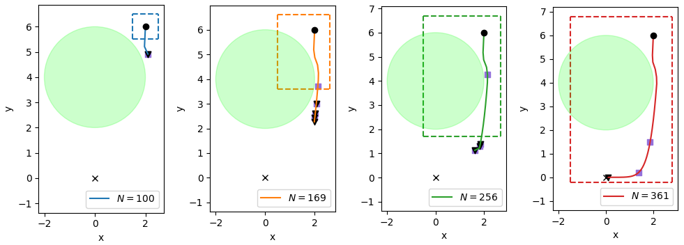
Figure 1: Safe stabilization of a planar system with worst-case uncertainty error bounds. The green ball is the unsafe set and black dots denote initial conditions. Dashed lines enclose the region where data is located for different $N$. Solid lines show the evolution under the corresponding CLF-CBF-SOCP controller in (15). Black triangles indicate points where the sufficient conditions for feasibility (10) in Proposition 4.2 do not hold. Purple squares denote points where the root-finding method (fsolve from Python’s SCIPY library) did not return a solution satisfying the sufficient condition of Proposition 4.5.

Performance dependency on error estimates: Here we illustrate how smaller estimation errors lead to improved performance. We use different datasets with different number of data points $N$ to generate $\hat{f}$, $\hat{g}$, $e_{f}$, and $e_{g}$. We solve the resulting CLF-CBF-SOCP every $0.01$s with initial condition at $(2.0,6.0)$ and plot the trajectories until it becomes unfeasible. We compare the results for different $N$ in Figure 1. Larger datasets with data from a neighborhood of the origin allow trajectories to converge closer to the origin before the problem becomes unfeasible. This illustrates one of the critical points of the paper: optimization-based control formulations that take uncertainty into account in order to ensure safety or stability might be unfeasible depending on the specific system and the magnitude of the errors in the employed approximations. Our results here provide quantifiable conditions to determine whether the accuracy of the approximations is sufficient or, instead, they need to be refined in order to guarantee feasibility. In the plot, we observe that the sufficient conditions in Propositions 4.2 and 4.5 serve as a good indicator of when the SOCP actually becomes unfeasible, hence illustrating how they can be used to infer when the available estimates are insufficient to guarantee that the controller is well defined.

Online safe stabilization: We illustrate also the case where data is collected online. We start from an initial set of 150 measurements of $f$, $g$ and $h$ near the initial condition obtained by querying the oracle. Given an initial condition, at every $0.01$s we check whether the conditions in (10) hold. If this is the case, we find the CLF-CBF-SOCP controller and execute it. If during the execution the conditions in (10) stop being satisfied at some point $\bar{x}$, we query the oracle to obtain measurements of $f$ and $g$ at $\bar{x}$ (making it feasible) and a small neighborhood around it (for improved performance). Figure 2 illustrates executions of this procedure for three different initial conditions. As trajectories approach the origin, more measurements need to be taken because the conditions in (10) become harder to satisfy.

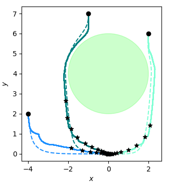
Figure 2: Safe stabilization of a planar system with worst-case uncertainty error bounds. The green ball is the unsafe set and black dots denote initial conditions. The solid lines display the evolution of the controller obtained by solving the CLF-CBF-SOCP (15). Black stars denote points where measurements have been taken. All trajectories asymptotically converge to a ball around the origin of radius 0.01. For reference, the dashed lines display the evolution of a min-norm controller with perfect knowledge of the dynamics, CBF and CLF (CLF-CBF QP) (Ames et al., 2017), for which the trajectories stay safe and asymptotically converge to the origin.

Time complexity: We show here the computational savings of checking the sufficient conditions in Propositions 4.2 and 4.5 as compared to directly solving the SOCP using the Embedded Conic Solver from the Python library CVXPY. Figure 3 shows that the time complexity of using the SOCP solver is higher than the time complexity of checking the sufficient condition in Proposition 4.5, which is in turn higher than the time complexity of checking the sufficient condition of Proposition 4.2. Since, in general, state-of-the-art SOCP solvers provide infeasibility and optimality certificates with the same time complexity, cf. (Domahidi et al., 2013, Section A), our sufficient conditions can be used to save computation time in the case where the problem is unfeasible, cf. Remark 4.8.

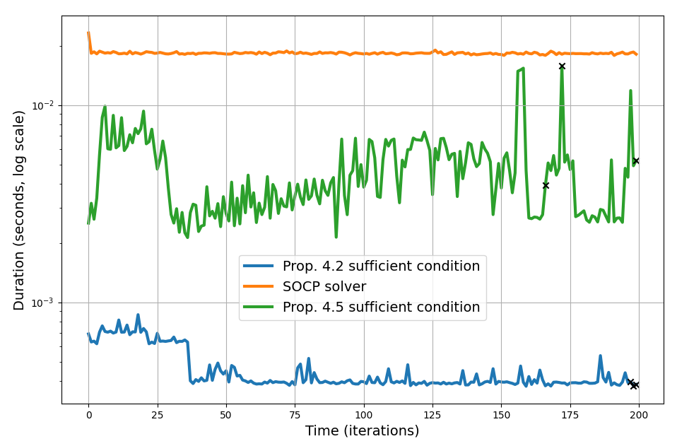
Figure 3: Time complexity comparison of evaluating the sufficient conditions in Proposition 4.2 (blue), Proposition 4.5 (green) and using an SOCP solver (orange) along the trajectory with $N=361$ in Figure 1. The black crosses denote points where the sufficient conditions do not hold. On average, the sufficient conditions in Proposition 4.2 is 50 times faster to evaluate than directly solving the SOCP.

7 Conclusions

We have studied conditions to ensure the safe stabilization of a nonlinear affine control system under uncertainty. Given either worst-case or probabilistic estimates of the dynamics, CBF and CLF, SOCCs encode the impact of uncertainty on the ability to guarantee stability and safety. We have provided conditions for the compatibility of the relevant pairs of SOCCs and provided explicit bounds on the error estimates that ensure these SOCCs are compatible. We have built on these results to ensure the existence of a smooth safe stabilizing controller, to show the point-Lipschitz and locally Lipschitz regularity of the min-norm CLF-CBF-SOCP-based controller, and to prove the regularity of a universal controller for the satisfaction of a single SOCC. Future work will characterize the conditions for compatibility in terms of data, design online safe stabilization mechanisms that balance computational effort, sampling rate, and performance using resource-aware control, explore the design of universal formulas for more than one SOCC, and implement our results on physical testbeds.

References

- Ahmadi and Majumdar (2016) A. A. Ahmadi and A. Majumdar. Some applications of polynomial optimization in operations research and real-time decision making. Optimization Letters, 10(4):709–729, 2016.
- Alizadeh and Goldfarb (2003) F. Alizadeh and D. Goldfarb. Second-order cone programming. Mathematical Programming, 95(1):3–51, 2003.
- Ames et al. (2017) A. D. Ames, X. Xu, J. W. Grizzle, and P. Tabuada. Control barrier function based quadratic programs for safety critical systems. IEEE Transactions on Automatic Control, 62(8):3861–3876, 2017.
- Ames et al. (2019) A. D. Ames, S. Coogan, M. Egerstedt, G. Notomista, K. Sreenath, and P. Tabuada. Control barrier functions: theory and applications. In European Control Conference, pages 3420–3431, Naples, Italy, 2019.
- Andréasson et al. (2020) N. Andréasson, A. Evgrafov, and M. Patriksson. An Introduction to Continuous Optimization: Foundations and Fundamental Algorithms. Courier Dover Publications, 2020.
- Artstein (1983) Z. Artstein. Stabilization with relaxed controls. Nonlinear Analysis, 7(11):1163–1173, 1983.
- Castañeda et al. (2021a) F. Castañeda, J. J. Choi, B. Zhang, C. J. Tomlin, and K. Sreenath. Pointwise feasibility of Gaussian process-based safety-critical control under model uncertainty. In IEEE Conf. on Decision and Control, pages 6762–6769, Austin, Texas, USA, 2021a.
- Castañeda et al. (2021b) F. Castañeda, J. J. Choi, B. Zhang, C. J. Tomlin, and K. Sreenath. Gaussian process-based min-norm stabilizing controller for control-affine systems with uncertain input effects and dynamics. In American Control Conference, pages 3683–3690, New Orleans, LA, May 2021b.
- Castañeda et al. (2022) F. Castañeda, J. J. Choi, W. Jung, B. Zhang, C. J. Tomlin, and K. Sreenath. Probabilistic safe online learning with control barrier functions. https://arxiv.org/pdf/2208.10733.pdf, 2022.
- Cortez and Dimarogonas (2021) W. S. Cortez and D. V. Dimarogonas. On compatibility and region of attraction for safe, stabilizing control laws. arXiv preprint arXiv:2008.12179, 2021.
- Dhiman et al. (2023) V. Dhiman, M. J. Khojasteh, M. Franceschetti, and N. Atanasov. Control barriers in Bayesian learning of system dynamics. IEEE Transactions on Automatic Control, 68(1):214–229, 2023.
- Domahidi et al. (2013) A. Domahidi, E. Chu, and S. Boyd. Ecos: An SOCP Solver for Embedded Systems. European Control Conference, pages 3071–3076, 2013.
- Horn and Johnson (2012) R. A. Horn and C. R. Johnson. Matrix Analysis. Cambridge University Press, 2012.
- Jankovic (2018) M. Jankovic. Robust control barrier functions for constrained stabilization of nonlinear systems. Automatica, 96:359–367, 2018.
- Long et al. (2021) K. Long, C. Qian, J. Cortés, and N. Atanasov. Learning barrier functions with memory for robust safe navigation. IEEE Robotics and Automation Letters, 6(3):4931–4938, 2021.
- Long et al. (2022) K. Long, V. Dhiman, M. Leok, J. Cortés, and N. Atanasov. Safe control synthesis with uncertain dynamics and constraints. IEEE Robotics and Automation Letters, 7(3):7295–7302, 2022.
- Long et al. (2023a) K. Long, Y. Yi, J. Cortés, and N. Atanasov. Safe and stable control synthesis for uncertain system models via distributionally robust optimization. In American Control Conference, pages 4651–4658, San Diego, California, June 2023a.
- Long et al. (2023b) K. Long, Y. Yi, J. Cortés, and N. Atanasov. Distributionally robust Lyapunov function search under uncertainty. In Conference on Learning for Dynamics and Control. Philadelphia, PA, 2023b.
- Mestres and Cortés (2023) P. Mestres and J. Cortés. Optimization-based safe stabilizing feedback with guaranteed region of attraction. IEEE Control Systems Letters, 7:367–372, 2023.
- Mestres et al. (2023) P. Mestres, A. Allibhoy, and J. Cortés. Robinson’s counterexample and regularity properties of optimization-based controllers. Systems & Control Letters, 2023. Submitted. Available at https://arxiv.org/abs/2311.13167.
- Ong (2022) P. Ong. Uniting and balancing control objectives: safety, stability, smoothness and resource conservation. PhD thesis, University of California, San Diego, 2022. Electronically available at http://terrano.ucsd.edu/jorge/group/data/PhDThesis-PioOng-21.pdf.
- Ong and Cortés (2019) P. Ong and J. Cortés. Universal formula for smooth safe stabilization. In IEEE Conf. on Decision and Control, pages 2373–2378, Nice, France, December 2019.
- Reis et al. (2021) M. F. Reis, A. P. Aguilar, and P. Tabuada. Control barrier function-based quadratic programs introduce undesirable asymptotically stable equilibria. IEEE Control Systems Letters, 5(2):731–736, 2021.
- Robinson (1980) S. M. Robinson. Strongly regular generalized equations. Mathematics of Operations Research, 5(1):43–62, 1980.
- Robinson (1982) S. M. Robinson. Generalized equations and their solutions, part II: Applications to nonlinear programming. In M. Guignard, editor, Optimality and Stability in Mathematical Programming, volume 19 of Mathematical Programming Studies, pages 200–221. Springer, New York, 1982.
- Sontag (1989) E. D. Sontag. A universal construction of Artstein’s theorem on nonlinear stabilization. Systems & Control Letters, 13(2):117–123, 1989.
- Sontag (1998) E. D. Sontag. Mathematical Control Theory: Deterministic Finite Dimensional Systems, volume 6 of TAM. Springer, 2 edition, 1998. ISBN 0387984895.
- Spivak (1995) M. Spivak. Calculus on Manifolds. Addison-Wesley Publishing Company, 1995.
- Srinivas et al. (2010) N. Srinivas, A. Krause, S. M. Kakade, and M. Seeger. Gaussian process optimization in the bandit setting: no regret and experimental design. arXiv preprint arXiv:0912.3995, 2010.
- Still (2018) G. Still. Lectures On Parametric Optimization: An Introduction. Preprint, Optimization Online, 2018.
- Taylor et al. (2019) A. J. Taylor, V. D. Dorobantu, H. M. Le, Y. Yue, and A. D. Ames. Episodic learning with control Lyapunov functions for uncertain robotic systems. In IEEE/RSJ Int. Conf. on Intelligent Robots & Systems, pages 6878–6884, Macau, 2019.
- Wang et al. (2017) L. Wang, A. Ames, and M. Egerstedt. Safety barrier certificates for collisions-free multirobot systems. IEEE Transactions on Robotics, 33(3):661–674, 2017.
- Wang (1974) P. S. Wang. The undecidability of the existence of zeros of real elementary functions. Journal of the ACM, 21(4):586–589, 1974.
- Wieland and Allgöwer (2007) P. Wieland and F. Allgöwer. Constructive safety using control barrier functions. IFAC Proceedings Volumes, 40(12):462–467, 2007.